active and passive flow control over the flight deck …mason/mason_f/dmshaferms.pdf · active and...

ACTIVE AND PASSIVE FLOW CONTROL OVER THE

FLIGHT DECK OF SMALL NAVAL VESSELS

Daniel M. Shafer

Thesis submitted to the Faculty of the

Virginia Polytechnic Institute and State University

in partial fulfillment of the requirements for the degree of

MASTER OF SCIENCE

in

Aerospace Engineering

APPROVED:

Dr. William H. Mason, chair

Dr. William Devenport

Dr. David B. Findlay

April 27, 2005

Blacksburg, Virginia

Keywords: helicopter/ship operations, frigate ship airwake, flow control,

backward facing step

ACTIVE AND PASSIVE FLOW CONTROL OVER THE

FLIGHT DECK OF SMALL NAVAL VESSELS

Daniel M. Shafer

ABSTRACT

Helicopter operations in the vicinity of small naval surface vessels often require

excessive pilot workload. Because of the unsteady flow field and large mean velocity

gradients, the envelope for flight operations is limited. This experimental investigation

uses a 1:144 scale model of the U.S. Navy destroyer DDG-81 to explore the problem.

Both active and passive flow control techniques were used to improve the flow field in

the helicopter’s final decent onto the flight deck. Wind tunnel data was collected at a set

of grid points over the ship’s flight deck using a single component hotwire. Results show

that the use of porous surfaces decreases the unsteadiness of the flow field. Further

improvements are found by injecting air through these porous surfaces, causing a

reduction in unsteadiness in the landing region of 6.6% at 0 degrees wind-over-deck

(WOD) and 8.3% at 20 degrees WOD. Other passive configurations tested include

fences placed around the hangar deck edges which move the unsteady shear layer away

from the flight deck. Although these devices cause an increase in unsteadiness

downstream of the edge of the fence when compared to the baseline, the reticulated foam

fence caused an overall decrease in unsteadiness in the landing region of 12.1% at 20

degrees WOD.

DEDICATION

This work is dedicated to my mother who passed away on January 31, 2005. She

suffered from breast cancer for four years, yet always kept a positive outlook on life. She

is an inspiration to all of us. She was loved greatly, is missed dearly, and will never be

forgotten. I love you mom!

iii

ACKNOWLEDGEMENTS

This investigation would not have been possible without the support of the NATO

AVT-102 task group. Great thanks goes to Terry Ghee for all the technical assistance,

guidance, and mentoring he provided during this academic endeavor. Colin Wilkinson

also provided guidance, contributed to the literature search and graphics, and helped me

keep in contact with everyone upon completion of the testing phase. Robin Imber

originally thought of the idea of testing the reticulated foam fence. Thanks to everyone in

the Advanced Aerodynamics branch at Naval Air Systems Command, Patuxent River,

MD for providing a friendly work environment, as I am happy to have had the

opportunity to provide a contribution to their work. Thanks also goes to Dr. Bill Mason,

my advisor, and Dr. Dave Findlay, head of the NAVAIR branch above. Without the

cooperation of these two people, this project could not have happened. Finally, the entire

faculty, staff, and Virginia Tech community have provided a graduate school experience

that I would not trade for anything.

This work would also not have been possible without the personal support from

my family and friends. My mother and father have provided more love and

encouragement over the years than seems possible. I can only hope to be as good of a

parent as they are. I have also always looked up to my big sister, Angela. Thank you all

for being good role models. Finally, I must thank Theresa for putting up with me during

all the stressful times in grad school. She made the experience much more enjoyable.

iv

TABLE OF CONTENTS

ABSTRACT………............................................................................................................ ii

DEDICATION……........................................................................................................... iii

ACKNOWLEDGEMENTS............................................................................................... iv

TABLE OF CONTENTS.................................................................................................... v

LIST OF FIGURES .......................................................................................................... vii

LIST OF TABLES…........................................................................................................ xii

NOMENCLATURE ........................................................................................................ xiii

1. INTRODUCTION AND BACKGROUND ................................................................. 1

1.1 Flow physics background ......................................................................................... 2 1.2 Airwake analysis....................................................................................................... 5 1.3 Thesis overview ........................................................................................................ 7

2. FLOW CONTROL TECHNIQUES ............................................................................. 9

2.1 Conditioning / filtering the airwake........................................................................ 11 2.2 Moving / deflecting the airwake ............................................................................. 12 2.3 Combined techniques.............................................................................................. 13 2.4 Device selection ...................................................................................................... 13

3. EXPERIMENTAL INVESTIGATION...................................................................... 17

3.1 Experimental setup.................................................................................................. 17 3.1.1 NATF wind tunnel ........................................................................................... 17 3.1.2 DDG model...................................................................................................... 18 3.1.3 Flow control devices ........................................................................................ 18 3.1.4 Data acquisition system ................................................................................... 21 3.1.5 Traverse system ............................................................................................... 21 3.1.6 Wind tunnel procedures ................................................................................... 23

3.2 Test plan.................................................................................................................. 23 3.3 Uncertainty / repeatability....................................................................................... 27

3.3.1 Measurement uncertainties .............................................................................. 27 3.3.2 Tie-in run ......................................................................................................... 28 3.3.3 Measurement system random uncertainty ....................................................... 28

4. RESULTS AND DISCUSSION: 0 DEGREES WIND-OVER-DECK...................... 33

4.1 Mean velocity.......................................................................................................... 33 4.1.1 Mean velocity contours.................................................................................... 33 4.1.2 Mean velocity line plots................................................................................... 37

4.2 Velocity standard deviation .................................................................................... 42

v

4.2.1 Velocity standard deviation contours............................................................... 42 4.2.2 Velocity standard deviation line plots.............................................................. 49

4.3 Turbulence intensity................................................................................................ 52 4.3.1 Turbulence intensity contour plots................................................................... 52 4.3.2 Turbulence intensity line plots......................................................................... 55

4.4 Average unsteadiness in landing area ..................................................................... 59 4.5 Frequency analysis.................................................................................................. 65

4.5.1 Calculation of frequency spectra ..................................................................... 66 4.5.2 Power spectral density discussion.................................................................... 69 4.5.3 Frequency-separated standard deviation contours ........................................... 72 4.5.4 Alternative frequency breakdown.................................................................... 75 4.5.5 Frequency analysis summary........................................................................... 75

5. RESULTS AND DISCUSSION: 20 DEGREES WIND-OVER-DECK.................... 77

5.1 Mean velocity.......................................................................................................... 78 5.1.1 Mean velocity contours.................................................................................... 78 5.1.2 Mean velocity line plots................................................................................... 79

5.2 Velocity standard deviation .................................................................................... 81 5.2.1 Velocity standard deviation contours............................................................... 81 5.2.2 Velocity standard deviation line plots.............................................................. 83

5.3 Turbulence intensity................................................................................................ 85 5.3.1 Turbulence intensity contours.......................................................................... 85 5.3.2 Turbulence intensity line plots......................................................................... 86

5.4 Average unsteadiness in landing area ..................................................................... 88 5.5 Frequency analysis.................................................................................................. 88 5.6 Comparison to 0 degrees WOD .............................................................................. 90

6. CONCLUSIONS AND RECOMMENDATIONS ..................................................... 95

REFERENCES…… ......................................................................................................... 98

APPENDIX A: CALCULATION OF STANDARD DEVIATION ............................. 101

APPENDIX B: DERIVATION OF RESULTANT MEAN VELOCITY FOR SINGLE

COMPONENT HOT WIRE ................................................................ 103

APPENDIX C: CONTOUR INTERPOLATION TECHNIQUE.................................. 105

APPENDIX D: POWER SPECTRAL DENSITY CALCULATION ........................... 108

VITA………………....................................................................................................... 111

vi

LIST OF FIGURES

Figure 1.1. Idealized flow over a backward facing step (Driver et al.7). ........................... 2

Figure 1.2. Simplified sketch of a ship’s rear landing deck and fluid structure. ............... 4

Figure 2.1. Venn diagram of the categorization of flow control devices. ......................... 9

Figure 2.2. Sketches showing how each flow control device can be used. ..................... 10

Figure 2.3. Side view of the rear portion of the model showing the raised flight deck... 14

Figure 2.4. Fence flow control configurations under investigation. ................................ 15

Figure 3.1. NAVAIR Aerodynamic Test Facility............................................................ 17

Figure 3.2. Image of ship model in NATF....................................................................... 18

Figure 3.3. Schematic of experimental setup................................................................... 18

Figure 3.4. Construction of the raised flight deck and hangar extension. Note that the

landing surface porous plate has not been installed yet. ........................................... 19

Figure 3.5. Float-type flow meter used to measure mass flow. ....................................... 19

Figure 3.6. Side view of how injection is distributed in the cavities. The circular baffle

(a) allows pressurization throughout the entire cavity. The diagonal baffle (b)

channels all air to the hangar face............................................................................. 20

Figure 3.7. Experimental data grid at 0 degrees yaw (a), and 20 degrees yaw (b) as

viewed looking upstream. ......................................................................................... 22

Figure 3.8. Sketch of the data plane................................................................................. 22

Figure 3.9. Differences between run 3 (left) and run 5 (right). ....................................... 24

Figure 3.10. Velocity standard deviation above the center landing spot for a baseline

model during (a) prior experiments and (b) current experiments. ............................ 28

Figure 3.11. Grid locations used to document the measurement system’s random error.29

Figure 3.12. Velocity running average of independent time histories at a single spatial

location in the freestream.......................................................................................... 31

Figure 3.13. Velocity running average of independent time histories measured on the

centerline at z/h = 0.34. ............................................................................................. 31

Figure 3.14. Velocity running average of independent 32-second time histories measured

on the centerline at z/h = 0.34. .................................................................................. 32

vii

Figure 4.1. Mean velocity of the baseline configuration (contours in % freestream); (a),

the entire flow field, and (b), the region of interest. ................................................. 34

Figure 4.2. Run 3 mean velocity...................................................................................... 35

Figure 4.3. Run 8 mean velocity...................................................................................... 36

Figure 4.4. Run 11 mean velocity.................................................................................... 37




Figure 4.8. Mean velocity at low hover (z/h = 0.66) for porous surface configurations . 39

Figure 4.9. Mean velocity at low hover (z/h = 0.66) for fence configurations. ............... 39

Figure 4.10. Mean velocity on the vertical centerline (2y/b = 0) for porous surface

configurations. .......................................................................................................... 40

Figure 4.11. Mean velocity on the vertical centerline (2y/b = 0) for fence configurations.

................................................................................................................................... 41

Figure 4.12. Velocity standard deviation of the baseline data; (a), the entire flow field,

and (b), the region of interest.................................................................................... 43

Figure 4.13. Velocity standard deviation of vented porous surface configuration (0.0625”

holes, run 3). ............................................................................................................. 44

Figure 4.14. Velocity standard deviation of non-vented porous surface configuration

(0.0625” holes, run 5). .............................................................................................. 44

Figure 4.15. Velocity standard deviation of non-vented porous surface configuration

(0.024” holes, run 6). ................................................................................................ 44

Figure 4.16. Velocity standard deviation of run 7 (injection using circular baffle). ....... 46

Figure 4.17. Velocity standard deviation of run 8 (injection from hangar face). ............ 46

Figure 4.18. Velocity standard deviation of run 9. .......................................................... 46

Figure 4.19. Velocity standard deviation of the serrated porous fence configuration (run

11). ............................................................................................................................ 47

Figure 4.20. Velocity standard deviation of the triangular-notched porous fence

configuration (run12). ............................................................................................... 47

Figure 4.21. Velocity standard deviation of porous “mini delta wing” configuration (run

13). ............................................................................................................................ 48

viii

Figure 4.22. Velocity standard deviation of solid “mini delta wing” configuration (run

14). ............................................................................................................................ 48

Figure 4.23. Velocity standard deviation of reticulated foam fence configuration (run

15). ............................................................................................................................ 48

Figure 4.24. Velocity standard deviation at low hover for porous surface configurations.

................................................................................................................................... 50

Figure 4.25. Velocity standard deviation at low hover for fence configurations. ........... 50

Figure 4.26. Velocity standard deviation along vertical centerline for porous surface

configurations. .......................................................................................................... 51

Figure 4.27. Velocity standard deviation along vertical centerline for fence

configurations. .......................................................................................................... 51

Figure 4.28. Turbulence intensity of the baseline configuration. .................................... 53

Figure 4.29. Turbulence intensity of run 3. ..................................................................... 54

Figure 4.30. Turbulence intensity of run 8. ..................................................................... 54

Figure 4.31. Turbulence intensity of run 11. ................................................................... 55




Figure 4.35. Turbulence intensity at low hover (z/h = 0.66) for porous surface

configurations. .......................................................................................................... 57

Figure 4.36. Turbulence intensity at low hover (z/h = 0.66) for fence configurations. ... 57

Figure 4.37. Turbulence intensity on the vertical centerline (2y/b = 0) for porous surface

configurations. .......................................................................................................... 58

Figure 4.38. Turbulence intensity on the vertical centerline (2y/b = 0) for fence

configurations. .......................................................................................................... 58

Figure 4.39. Baseline velocity standard deviation. The box encloses the region in the

airwake which affects helicopter operations............................................................. 60

Figure 4.40. Percent change of the average unsteadiness in the landing region with

respect to the baseline. .............................................................................................. 62

Figure 4.41. Width changes to the landing region ( |2y/b| = 1, 1.4, 1.7) overlaid on the

velocity standard deviation contour plot................................................................... 63

ix

Figure 4.42. Height changes to the landing region (z/h = 1.9, 2.4, 2.9) overlaid on the

velocity standard deviation contour plot................................................................... 63

Figure 4.43. Bar graph showing the effect of widening the landing area. ...................... 64

Figure 4.44. Bar graph showing the effect of raising the height of landing area............. 65

Figure 4.45. Diagram of how data was divided to produce the PSD............................... 67

Figure 4.46. Effect of averaging several individual PSDs............................................... 68

Figure 4.47. Effect of passing the PSD through a low-pass digital filter (smoothed). .... 68

Figure 4.48. PSDs of selected configurations at: a) z/h = 0.66 and 2y/b = 0; b) z/h = 0.66

and 2y/b = 1.37.......................................................................................................... 69

Figure 4.49. Velocity spectra following Kolmogorov’s hypothesis. ............................... 71

Figure 4.50. Ratio of the standard deviation due to low frequencies to the total standard

deviation for the baseline configuration. .................................................................. 72

Figure 4.51. Baseline velocity standard deviation for: (a) the 0 – 125 Hz domain; (b) the

125 – 2000 Hz domain.............................................................................................. 73

Figure 4.52. Velocity standard deviation for the porous flight deck with blowing from

the hangar face for: (a) the 0 – 125 Hz domain; (b) the 125 – 2000 Hz domain. .... 74

Figure 4.53. Velocity standard deviation for the porous serrated fence configuration for:

(a) the 0 – 125 Hz domain; (b) the 125 – 2000 Hz domain. ..................................... 74

Figure 5.1. Mean velocity for the 20 degrees WOD baseline configuration. The contours

are in percent of freestream velocity......................................................................... 78

Figure 5.2. Mean velocity of reticulated foam fence configuration (run 17). ................. 79

Figure 5.3. Mean velocity of porous surfaces with injection configuration (run 18). ..... 79

Figure 5.4. Mean velocity at low hover (z/h = 0.66) for 20 degrees WOD case. ............ 80

Figure 5.5. Mean velocity near the vertical centerline (2y/b = 0.23) for 20 degrees WOD

case............................................................................................................................ 81

Figure 5.6. Velocity standard deviation for the 20 degrees WOD baseline configuration.

The contours are in percent of freestream velocity................................................... 82

Figure 5.7. Velocity standard deviation of reticulated foam fence configuration ........... 82

Figure 5.8: Velocity standard deviation of porous surfaces with injection configuration82

Figure 5.9. Velocity standard deviation at low hover (z/h = 0.66) for 20 degrees WOD

case............................................................................................................................ 84

x

Figure 5.10. Velocity standard deviation near the vertical centerline (2y/b = 0.23) for 20

degrees WOD case.................................................................................................... 84

Figure 5.11. Turbulence intensity for the 20 degrees WOD baseline configuration. ...... 85

Figure 5.12. Turbulence intensity of the reticulated foam fence configuration (run 17). 86

Figure 5.13. Turbulence intensity of the porous surfaces with injection configuration (run

18). ............................................................................................................................ 86

Figure 5.14. Turbulence intensity at low hover (z/h = 0.66) for 20 degrees WOD case. 87

Figure 5.15. Turbulence intensity near the vertical centerline (2y/b = 0.23) for 20 degrees

WOD case. ................................................................................................................ 87

Figure 5.16. Baseline velocity standard deviation for the 20 degrees WOD runs:.......... 89

Figure 5.17. Velocity standard deviation at 20 degrees WOD for the porous flight deck

with blowing from the hangar face for: a) the 0 – 125 Hz domain; b) the 125 – 2000

Hz domain................................................................................................................. 90

Figure 5.18. Velocity standard deviation at 20 degrees WOD for the reticulated foam

fence configuration in: a) the 0 – 125 Hz domain; b) the 125 – 2000 Hz domain. . 90

Figure 5.19. Comparison of mean velocity at 0 and 20 degrees WOD at z/h = 0.66. ..... 92

Figure 5.20. Comparison of standard deviation at 0 and 20 degrees WOD at z/h = 0.66.

................................................................................................................................... 92

Figure 5.21. Comparison of mean velocity at 0 and 20 degrees WOD near the vertical

centerline................................................................................................................... 94

Figure 5.22. Comparison of standard deviation at 0 and 20 degrees WOD near the

vertical centerline...................................................................................................... 94

xi

LIST OF TABLES

Table 2.1. Matrix of flow control devices........................................................................ 10

Table 3.1. Run log for wind tunnel experiments. ............................................................ 26

Table 4.1. Average unsteadiness of each configuration. ................................................. 62

xii

NOMENCLATURE

Constants

Symbol Name Value

h Height of hangar 1.0 in

b Beam of ship at the landing spot 4.375 in

Variables

Symbol Name Units

x Streamwise coordinate in

y Lateral coordinate in

z Vertical coordinate in

m& Mass flow ft3/min

∞U Freestream velocity ft/s

u Unsteady freestream velocity component ft/s

v Unsteady lateral velocity component ft/s

w Unsteady vertical velocity component ft/s

σ Velocity standard deviation ft/s

µ Turbulent normal stress (ft/s)2

TKE Turbulent kinetic energy (ft/s)2

TI Turbulence intensity -

localU Local mean velocity ft/s

WOD Wind-over-deck angle degrees

xiii

1. INTRODUCTION AND BACKGROUND

As long as helicopters have been flying, it has been desirable to land them aboard

ships at sea. When these helicopter/ship operations began several decades ago, little was

known about the unsteady airwake through which the helicopter must maneuver to land.

Consequently, flight operations around small naval vessels have historically been one of

the most difficult skills for a helicopter pilot to master. Even with years of experience, a

pilot cannot completely anticipate how the unsteady airwake behind a ship will behave.

Over the years numerous accidents have occurred during flight operations, causing lives

to be lost and millions of dollars of damage. As a result, efforts to characterize and

predict the flow behavior due to the ship airwake began more than a decade ago.1, 2

Although studies on the subject have become more common in recent years, little

knowledge exists on ways to control and reduce the unsteady wake that helicopters

encounter in this situation. Consequently, the existing knowledge of the physics of ship

airwakes should be examined to find a solution which reduces airwake turbulence and

allows for safer helicopter/ship operations over a wider range of flight conditions.

Most current small naval ships were designed without considerations for the

airwake encountered during takeoff and landing maneuvers. Although airwake analysis

is now an important part of new ship designs, an effort must also be made to increase the

safety of personnel on those vessels currently in the fleet. This investigation focuses on

finding techniques which improve the airwake over the rear landing deck of frigate-type

ships, specifically the DDG class.

- 1 -

1.1 Flow physics background

In its most basic form, flow over the rear landing deck aft of the hangar on

frigate-type ships can be thought of as flow over a backward facing step. Experimental

and computational literature is readily available for two dimensional versions of this

flow.3, 4, 5, 6, 7, 8, 9 Figure 1.1 illustrates the general characteristics of this two dimensional

flow. The dominant flow feature is the large recirculation region beneath the unsteady,

separated shear layer. This shear layer acts like a mixing layer, as coherent structures are

formed and transported downstream initially. However, the lives of these structures are

very short since they breakup prior to reattachment to the surface. Because this process is

chaotic, reattachment is not stationary and must be characterized by a region, not a point.

This is one of the reasons why helicopter landings are difficult; the landing spot is near

this reattachment region.

Figure 1.1. Idealized flow over a backward facing step (Driver et al.7).

- 2 -

Although this fundamental understanding of two dimensional flow over a

backward facing step is available, its applicability to flight deck flow fields is limited.

There are two primary concerns. First, the flow over a ship is far from two dimensional,

as the ratio of beam width to step height is approximately three. This aspect ratio is an

important parameter in flows with massive separation regions,10 and the three

dimensionality is important in this application. A second reason for the limited

applicability involves the condition of the oncoming flow. Because of upstream bodies

on the ship (stacks, antennas, mast, etc.), the flow over the step is not uniform. This

complicates matters as the oncoming flow is completely unsteady and nearly impossible

to quantify. As a result, analyzing simplified models of this type of flow may not be

particularly useful.

Extending the backward facing step flow to three dimensions, consider flow

perpendicular to the top hangar edge. Literature11, 12, 13 suggests the characteristics shown

in Figure 1.2, discovered though extensive flow visualization. Similar to the two

dimensional case, a large recirculation region exists behind the step; however, this flow

field is no longer two dimensional. On the flight deck, flow is incoming from the sides of

the ship causing counter-rotating vortices on each side of the recirculation region. This

results in a horseshoe vortex structure. Keep in mind, however, that this structure is not

stationary. As a result, the natural unsteadiness of the flow causes this structure to grow,

dissipate, and move spatially in an unpredictable manner.

- 3 -

Horseshoe vortex

Reattachment line

Hanger face

Flight deck

Figure 1.2. Simplified sketch of a ship’s rear landing deck and fluid structure.

Adding another degree of complexity, one must also consider situations when the

freestream has a crosswind component. These nonzero wind-over-deck (WOD) angles

(or yaw angles) occur quite frequently, as it is rare for a ship to be cruising on a heading

such that the WOD is directly down the centerline. As a result, these situations require

study. The literature11, 12, 13 also characterizes the flow around frigate-type ships at

several WOD angles. Again, various types of flow visualization were used to define a

flow model in the vicinity of the landing deck on the ship. Rhoades11 showed that at

moderate WOD angles (approximately 45 degrees), large coherent structures are shed

from the side edge of the hangar at regular intervals. Unfortunately, documentation of

this phenomenon on full scale ships is not available. However, this type of predictable

periodicity may not even occur at full scale for several reasons. First, models in a wind

- 4 -

tunnel are typically scaled down in size substantially. As with any bluff body, these

flows are Reynolds number and Strouhal number dependent, and the large scaling factors

are of concern. Additionally, the preexisting atmospheric boundary layer and turbulence

are infrequently modeled. It has been shown that accounting for these features is critical

when WOD angles approach 90 degrees.14

In summary, the simplified two and three dimensional backward facing step flows

provide a good physical overview of the flow encountered over the flight deck of frigate-

type ships. Recall that helicopter operations are difficult because the entire recirculation

region is unsteady and the landing spot on the flight deck is near the shear layer

reattachment region. Because of the flow field’s unsteadiness, a helicopter could be

inside the recirculation region at one instant, experiencing certain forces and moments,

only to be subjected to an unrecoverable yawing moment outside the recirculation region

at the next instant. Thus, to reduce pilot workload, it is desirable to decrease flow

gradients and remove as much of the flow field unsteadiness as possible over the flight

deck.

1.2 Airwake analysis

Recently, with the development of more advanced CFD methods and increased

computing power, numerical simulations and capabilities have dramatically improved.

Results from CFD solutions for ship airwakes are available in the literature.15, 16, 17, 18

Solutions often use time-accurate calculations and agree with wind tunnel and flight test

data fairly well. In one case19 the CFD solution is used with a flight simulator enabling a

pilot to fly through the airwake. This gives the pilot the ability to determine how realistic

- 5 -

the solution model is. Thus, CFD has shown some success and will continue to improve

as the technology advances in the future. These simulations can accomplish two main

tasks for a fraction of the cost of full scale flight test. First, pilots are able to train in

simulators in a wide variety of unique ship airwakes. Allowing training in a simulator

will better prepare pilots for actual landings aboard ships and decrease the amount of

actual flight time needed to develop these skills. It is also anticipated that manned flight

simulations will be used to define the helicopter/ship operating envelope. Every time an

aircraft or ship design is modified, the operating envelope must be redefined. Currently

the only way to do this is by actual flight test, and although simulations are not intended

to be a replacement, the number of test points can be greatly reduced using simulations.

This will result in significant time and cost savings.

Wind tunnel experiments can also aide in airwake analysis. In addition to the

flow physics experiments mentioned above, other researchers have mapped the flight

paths of the aircraft approach to different ships.20, 21 This wind tunnel data was used not

only for a better understanding of the flow field, but also for CFD validation and an

airwake model in a flight simulator. Other wind tunnel experiments22 measuring

unsteady forces and moments on a helicopter fuselage show promise in predicting the

operating limits for helicopter operations. By correlating the magnitudes of these

unsteady fluctuations to pilot workloads from full scale flight test, operating envelopes

were approximated. Again, by minimizing the amount of flight test, time and money can

be saved. It has also been shown that rotor downwash has a significant effect on the flow

field,23 and the flow field over the landing deck causes a decrease in rotor thrust.24 Thus,

to get the most realistic results from ship airwake experiments, one must model the

- 6 -

helicopter fuselage, including the rotor. Finally, ship motion can also affect the airwake.

The unsteady six degree-of-freedom movements of the ship result in much greater flow

field complexities, and little documentation of this effect is available.25

Because the helicopter/ship interface is such a complex problem and much effort

has been placed on attempting to understand the phenomenon, efforts to actually “fix” the

problem have been insufficient. Although a large amount of information is available for

backward facing step flows, these works are rarely applied to small ship flow fields.

However, it was shown that porous fences can be used to significantly reduce

unsteadiness and decrease the mean velocity downstream of the step in two related

studies.26, 27 Though the studies’ motivation came from the helicopter/ship dynamic

interface problem, only two dimensional configurations were explored. Consequently,

much work and effort needs to be conducted in this flow control application. Presently,

an increased interest from around the world has resulted in support from NATO to

explore the problem in greater detail. With the existing knowledge of the physics of ship

airwakes, it is hoped that flow control techniques can be designed to increase the safety

and expand the operating limits of helicopter/ship operations. In conclusion, this

investigation is just the first step in developing these flow control techniques. Many of

the secondary effects (atmospheric boundary layer, rotor downwash, ship motion, etc.)

mentioned above are not considered.

1.3 Thesis overview

The next chapter introduces the many different techniques that can be used to

modify and reduce the flow field nonuniformity and unsteadiness over the flight deck of

- 7 -

frigate-type ships. This leads to a discussion of the specific techniques chosen for this

investigation. Chapter 3 explains the experimental setup, procedures, and the

instrumentation used to collect data. A composite test plan and run log is presented along

with an in depth uncertainty analysis of the entire hotwire measurement system. Chapter

4 contains the experimental results for configurations at 0 degrees wind-over-deck

(WOD). The majority of the investigation was spent evaluating flow control techniques

at this WOD angle. Several different types of analysis are discussed as there is no

specific metric widely accepted for evaluation of flow control devices at this time. In

Chapter 5, the two best control techniques from the 0 degree WOD cases are tested at 20

degrees WOD. A comparison between these two types of flow is also included. Finally,

the summary and conclusions are found in Chapter 6. Several recommendations are

made for future studies.

- 8 -

2. FLOW CONTROL TECHNIQUES

Numerous flow control techniques have been considered and fall into two broad

categories. First, the flow can be conditioned or filtered in some way as it passes over the

backward facing step and landing deck. The goal is to remove some of the energy in the

flow or possibly shift the magnitude of the unsteadiness in the frequency domain. The

other category involves devices which physically move or deflect the shear layer. The

motivation for this concept is to move highly turbulent flow out of the region in which

helicopters operate. Figure 2.1 is a diagram of how several novel devices fit into these

two categories. Note that some devices fit into both categories. Table 2.1 is a tabulated

version which includes references to sketches of the devices shown in Figure 2.2.

Blowing

Porous ship surfaces

Vortex generators

Multiple lateral wedges

Columnar vortex generators

Turning vanes

Ramp

Solid fence

Splitter plates

Porous fence

Serrated fence

Flexible skirt

Notched fence

Reticulated foam fence

Condition / Filter Airwake

ObjectiveReduce unsteadiness in the flow

and/or eliminate undesirable features

Move / Deflect Airwake

ObjectiveTransport undesirable fluid structures

to region of lesser importance

Figure 2.1. Venn diagram of the categorization of flow control devices.

- 9 -

Table 2.1. Matrix of flow control devices

Category Desired effect Control device / technique

1. Blowing 2. Porous ship surfaces 3. Vortex generators

Condition / filter airwake

Reduce unsteadiness in the flow and/or

eliminate undesirable features 4. Multiple lateral wedges

5. Porous fence 6. Serrated fence 7. Flexible skirt 8. Notched fence

Both

9. Reticulated foam fence 10. Columnar vortex generators 11. Turning vanes 12. Ramp 13. Solid fence

Move / deflect airwake

Transport undesirable fluid structures to region

of lesser importance

14. Splitter plates

1 2 3 4

5 6 7 8

12 13 14

9

10 11

Figure 2.2. Sketches showing how each flow control device can be used.

- 10 -

2.1 Conditioning / filtering the airwake

Ideally, all the devices in Figure 2.2 require test and evaluation; however, some

are believed to perform better than others by simply considering the physics of the flow.

First, the condition/filter category is considered. Literature suggests that a porous surface

downstream of a backward facing step can decrease the unsteadiness in the recirculation

region and lower the amount of reversed flow.28, 29 Porous surfaces allow the passage of

local high pressures to areas of low pressure, thus decreasing the magnitude of the

fluctuations on the surface. In addition to reducing the peak RMS pressure fluctuations,

particle image velocimetry (PIV) vector fields show shrinkage of the recirculation region.

While these were two-dimensional studies, the concept of “damping” the flow field near

the surface of the flight deck is applicable here. To further improve the flow field with

this configuration, the cavity beneath the porous surface could also be pressurized,

resulting in mass injection into the freestream. Because of the natural low pressure

region below the step,13 providing a positive mass flow here helps alleviate pressure

gradients. Furthermore, if the injection were in the direction of the freestream (out of the

vertical face of the step as shown in configuration 1 in Figure 2.2), energy would be

added in the direction of the velocity deficit.

The remaining two devices in this category could actually increase the

unsteadiness. Although vortex generators are commonly used to keep flow attached and

prevent wakes from developing, they are primarily used on streamlined objects which

require energy be added to the boundary layer. In this application, the upstream flow is

already chaotic due to the airwake of upstream bluff bodies (the ship’s mast, stacks,

antennas, etc.). Although vortex generators could possibly improve the flow by breaking

- 11 -

up large eddies and shifting the turbulent kinetic energy to a higher frequency domain,

this method was not pursued.

Another method to condition the airwake, not included in the sketches, is to use

active unsteady devices. Differing from constant uniform injection, these techniques

have a time dependent effect on the flow field. Perhaps the rotation speed of a wind

turbine is varied or a pulsed jet is used to decrease the magnitude of the unsteady

fluctuations. Creative techniques like these represent a completely new class of flow

control devices yet to be explored in this application.

2.2 Moving / deflecting the airwake

Now consider the move/deflect category. These techniques attempt to physically

move the unsteady shear layer in two basic ways. Solid fences, ramps, and columnar

vortex generators (CVGs)30 move the shear layer away from the region of helicopter

operations. Although these devices can decrease the unsteadiness in some regions, the

intensity of the shear layer or unsteadiness is often greatly magnified in other regions,

specifically downstream of the fence edge. Turning vanes and splitter plates attempt to

move the shear layer down towards the flight deck. However, other current research31

shows that these techniques may be completely nullified by the interaction of rotor

downwash. This dynamic interface has effects on all devices, but may be more

significant on devices which attempt to move the flow vertically. Experimentally

determining this interaction is difficult due to the need of a high fidelity, fully functioning

rotor model to place into the flow field.

- 12 -

2.3 Combined techniques

Thus far, all the devices and techniques discussed have fallen solely into either

one category or the other. Most of these devices have advantages and disadvantages. As

a result, it seems natural to attempt to combine the strategies of both categories. This

leads to the devices cited in the middle of Figure 2.1 and Table 2.1. This blended

category consists mainly of fences which are either non-rectangular or porous. By

shaping a solid rectangular fence to promote mixing, the severity of the shear layer

initiated at the top of the fence is reduced. In other words, if the fence is not rectangular,

the shear layer will be broken up as it is deflected. In addition, the flow could also be

“filtered” by using porous materials. This idea is inspired by the use of screens and

honeycomb in wind tunnels to reduce turbulence. Two materials which can be used are

porous sheet metal and reticulated foam (configurations 5 and 9 respectively in Figure

2.2). Using these two philosophies – shaping and porosity – several unique fences were

selected for testing.

2.4 Device selection

Because it is not possible to test every type of technique listed in Table 2.1, a few

of the most appealing were selected and explored in depth. Because multiple sources28, 29

have shown flow improvements with the use of porous surfaces, this technique was

explored in greater detail. To establish a better understanding of how porosity affects the

flow field, several different configurations were tested using this technique. Upon the

fabrication of such configurations, it is noted that the original DDG model is modified

with a raised flight deck (see Figure 2.3). This was essential to allow a cavity beneath the

- 13 -

porous surface. As a result, it was necessary to document the effect of “venting” the

cavity. More specifically, the original sidewalls of the cavity were constructed using

porous material, but data was also taken with solid cavity walls. Additionally, the effect

of hole diameter was explored as the porosity of the surfaces was held constant at 23%.

After these passive techniques were explored, blowing was added to the system.

Injection could be used in a variety of ways, but was used here to attempt to pressurize

the cavities. Further details of individual configurations are discussed in Section 3.1.3.

Raised Flight Deck

Hanger Extension

VData Plane

Waterline

Figure 2.3. Side view of the rear portion of the model showing the raised flight deck.

Fence devices were also explored. For the reasons discussed previously, focus

was placed on fences falling into both categories in Table 2.1. It has been shown that

porous fences cause a less severe shear layer than a solid fence with the same

dimensions.32 Referring to Figures 2.4a and b, the serrated porous fence and triangular-

notched porous fence attempt to break up the shear layer into smaller sized eddies and

deflect the remaining shear layer away from the flight deck. Figures 2.4c and d show

triangular-notched fences that are deflected 60 degrees upstream. The motivation for this

configuration comes from the natural characteristics of delta wings at high angles of

attack. It is hypothesized that tiny leading edge vortices develop and break up larger

scale eddies, leaving much smaller, higher frequency structures in the flow over the deck.

- 14 -

This is a desirable characteristic because low frequency unsteadiness is the main cause of

handling quality problems for pilots.33 Finally, Figure 2.4e consists of a reticulated foam

fence. The material is commercially available and is commonly used for padding and

sound absorbing. A triangular cross-section was chosen in an attempt to blend the shear

layer smoothly into the pre-existing airwake. In other words, the thickness of the fence

decreases with height. Note that the fences were placed around the edges of the hangar,

including the sides.

a. Serrated porous fence.

b. Triangular-notched porous fence.

c. Triangular-notched porous fence, angled 60

degrees upstream.

d. Triangular-notched solid fence, angled 60

degrees upstream.

Figure 2.4. Fence flow control configurations under investigation.

- 15 -

e. Reticulated foam fence.

Figure 2.4. Fence flow control configurations under investigation.

- 16 -

3. EXPERIMENTAL INVESTIGATION

3.1 Experimental setup

3.1.1 NATF wind tunnel

The wind tunnel tests were conducted at the NAVAIR Aerodynamic Test Facility

(NATF)34 in Patuxent River, Maryland. The NATF is a 4-foot by 4-foot closed test

section, open-return wind tunnel (see Figure 3.1). The facility incorporates a 200

horsepower motor that drives a variable pitch fan and delivers a maximum velocity of

205 feet per second. In addition, the wind tunnel has honeycomb and three sets of flow

conditioning screens that minimize freestream turbulence intensity to approximately

0.80% and freestream velocity variations of 1% or less.

Flow direction

Test section

Figure 3.1. NAVAIR Aerodynamic Test Facility.

- 17 -

3.1.2 DDG model

The model of the 1:144 scale DDG-81 ship, manufactured by NASA Langley

Research Center using stereo lithography techniques, was approximately 42 inches in

length. The beam of the ship on the rear flight deck varied from 4.9375 inches at the

hangar face to 3.5625 inches at the back edge of the ship. The model was affixed to a

boundary layer plate (Figure 3.2 and 3.3), 62 inches in length by 46.5 inches in width,

and was mounted in the tunnel 8 inches above the test section floor. An aerodynamic

profile was attached to the nose and trailing edge of the boundary layer plate. The

trailing edge piece was mounted upside down relative to the nose to assist wake

mitigation and recovery. A trip strip, composed of 1/8 inch wide, 80 grit sand paper was

glued to the leading edge of the boundary layer plate on the lower (7/8 inch downstream

from the leading edge) and upper surface (1/4 inch downstream from the leading edge).

Figure 3.2. Image of ship model in NATF.

Figure 3.3. Schematic of experimental setup.

8’

Tunnel center line

Velocity4’

3.1.3 Flow control devices

Sheet metal with two different sizes of machined holes served as the porous

surfaces. The raised flight deck and hangar extension were shaped to lay flush on the

- 18 -

existing DDG model and were elevated by affixing the surface to small cubes (3/8 inch)

as seen in Figure 3.4. The hangar face was constructed in a similar manner. Note that

aluminum tape can be placed on any porous surface to simulate the solid surfaces

discussed in the device selection section. Also note the hole in the original flight deck

surface just aft of the hangar. This ½ inch diameter hole extended through the model and

ground plane so that an airline could be installed for active flow control configurations.

The location on the landing deck for this airline port was on the centerline of the flight

deck one inch aft of the hangar face, chosen for the location of minimum pressure.13 A

1/8 inch diameter tube was then fitted to the bottom of the model. The tube exited the

tunnel under the boundary layer plate and passed through a mass flow meter which used

shop air as the pressure source. The regulator pressure was set nominally to 90 pounds

per square inch, but airflow was controlled by the float-type flow meter shown in Figure

3.5.

Figure 3.4. Construction of the raised flight deck and hangar extension. Note that the landing surface porous plate has not been installed yet.

Figure 3.5. Float-type flow meter used to measure mass flow.

- 19 -

Assuming constant density, the average velocity across a porous surface could be easily

calculated from:

AVm ρ=•

The blowing configurations were tested with a mass flow of 4 cubic feet per minute, the

maximum flow rate available with the setup. Given the area of the porous surfaces, the

injection could ideally occur at less than 0.5% of freestream velocity across the entire

surface. However, when the flow reached the plenum (the cavity below the porous

surfaces), a uniform pressure distribution was difficult to obtain since the jet of air

emptied into a relatively small volume. Two different techniques were used to solve this

problem. The first technique used a circular baffle placed ¼ inch above the injection

nozzle (Figure 3.6a). However, because the injected airflow acted on such a large surface

area, the low injection velocity caused little effect to be noticed. Consequently, the other

strategy was to pressurize only the hangar extension volume (Figure 3.6b). Given the

area of this porous surface alone, the injection was 2.5% of freestream velocity. This

(a) (b)

Figure 3.6. Side view of how injection is distributed in the cavities. The circular baffle (a) allows pressurization throughout the entire cavity. The diagonal baffle (b) channels all air to the hangar face.

- 20 -

higher velocity had a greater effect on the flow, and because injection was in the direction

of the freestream, momentum was added to help alleviate the velocity deficit.

The fences were also constructed of porous sheet metal and shaped with a variety

of metalworking tools. Each fence had a height of ½ inch. However, note that since

some of these fences were angled 60 degrees upstream, they were only ¼ inch in vertical

height. Finally, the commercially available reticulated foam was easily cut with scissors.

3.1.4 Data acquisition system

Thermal anemometry was used to acquire data. A single wire probe was used to

determine the resultant velocity time history. A single wire probe has the disadvantage of

having a velocity direction ambiguity but the advantage of sensing velocity without

limitation to flow angle. This becomes particularly important behind objects that exhibit

bluff body separation and recirculation. The probe was oriented such that the resultant of

the freestream and vertical components of velocity were measured. A Thermal Systems,

Inc. IFA 100 Flow Analyzer and ThermalPro Software were used to acquire and analyze

the data.

3.1.5 Traverse system

A Velamax two-component traverse was used to move the probe for data

acquisition. Data was acquired from 17 inches above the boundary layer plate and 8

inches on either side of the model centerline for the ship yawed 0 degrees to the flow, see

Figure 3.7a. With the ship yawed starboard 20 degrees, the grid was traversed across the

tunnel from 16 to –5 inches, see Figure 3.7b. To capture the ship wake, a spatial

- 21 -

resolution of one inch was used in the region behind the ship with an increased resolution

directly downstream of the backward facing step as shown in Figure 3.7. The axial

position analyzed was at the center of the flight deck, see Figure 3.8. This position was

3.0625 inches aft of the hangar face, or 3.0625h. Data was acquired at 4000 Hz (low-

pass filtered to 2000Hz) for 4 seconds at each grid point. Because the ship wake effect

on landing helicopters was the primary interest, the center of rotation of the ship (used to

change yaw angles) was located near the center of the flight deck.

0

2

4

6

8

10

12

14

16

18

-10 -8 -6 -4 -2 0 2 4 6 8 10

Spanwise Location (in)

Vert

ical

Loc

atio

n (in

)

0

2

4

6

8

10

12

14

16

18

-10 -8 -6 -4 -2 0 2 4 6 8 10 12 14 16

Spanwise Location (in)

Vert

ical

Loc

atio

n (in

)

(a) (b)

Figure 3.7. Experimental data grid at 0 degrees yaw (a), and 20 degrees yaw (b) as viewed looking upstream.

Figure 3.8. Sketch of the data plane.

- 22 -

3.1.6 Wind tunnel procedures

The tunnel was allowed to thermally stabilize for at least 20 minutes before data

acquisition commenced. The tunnel conditions were set to 75 feet per second, however,

due to the blockage effect of the traverse system, and to a lesser extant, the boundary

layer plate and mounting supports, the actual velocity near the model was slightly higher.

Tunnel temperature stabilized at 78.3 degrees Fahrenheit. Tunnel test conditions

(velocity, temperature, pressure, etc.) were acquired in addition to the thermal

anemometry data. The number of data points acquired was 239 for the 0 degree WOD

case and 287 for the 20 degree WOD case (Figure 3.7). The data were acquied in a top-

to-bottom, starboard-to-port pattern.

3.2 Test plan

Testing began by validating the setup with a tie-in run (Section 3.3.2). After this

was completed, data were collected on the baseline configuration that included the solid

raised flight deck and hangar extension as shown in the sketch in Figure 2.3. Note that

the first 15 runs were conducted at 0 degrees wind-over-deck (WOD) angle. Refer to

Table 3.1 for complete descriptions of the entire test.

The first objective of the test was to show that porous surfaces can be used to

remove unsteadiness in the flow (run 3). Next, the effects of “venting” the porous flight

deck were determined by comparing runs 3 and 5. Figure 3.9 shows the difference

between theses two configurations. (Note: Run 4 was invalid due to an incorrect setup.)

The size of the holes was also subject to investigation. As a result, the porous surfaces in

run 6 had holes which were about 1/3 the diameter of the prior porous material. Next,

- 23 -

active configurations were considered by adding injection to the passive configuration

which showed the most improvement. As seen in the run log, and will be seen in the

results, the porous material used here had the smaller diameter holes, and the sides of the

raised flight deck and hangar extension were solid (sealed with aluminum tape).

Porous sides Solid sides

Figure 3.9. Differences between run 3 (left) and run 5 (right).

The active configurations investigated used two different strategies as mentioned

above. First, in run 7, the circular baffle was tested. Then, the configuration which

injected air only from the hangar face was tested in run 8. Finally, run 9 determined how

injection affects the flow if the flight deck is solid.

Upon completion of testing the configurations which used porous surfaces, data

was taken again on the baseline model. There were two reasons for this. First, some

concerns had arisen during prior runs with respect to random errors and the uncertainty of

the hot wire measurement system. To remedy the situation, run 10 collected data at

several grid points on the baseline configuration again. At each point, several time

histories of differing length were recorded. Analysis of this data is found in Section

- 24 -

3.3.3. The other purpose for this run was to verify that data is repeatable with the first

baseline dataset.

Runs 11 to 15 collected data on the remaining configurations (the fences)

introduced in Section 2.4. Motivation for using each device was stated above, as porous

fences alleviate the increasing severity of the shear layers. Although most fences were

porous, a solid version of the triangular-notched fence angled 60 degrees upstream (“mini

delta wings”) was tested. Constructing this device with solid sheet metal may better

allow the formation of the leading edge vortices (run 14).

All wind tunnel runs discussed to this point were conducted at 0 degrees WOD.

Realizing that the most difficult conditions for helicopter operations are not necessarily at

this flow angle, a limited number of runs were conducted at 20 degrees WOD. Due to

time constraints, only two configurations, besides a new baseline, were tested. As a

result, the configuration which showed the most improvement using porous surfaces was

chosen, along with the most favorable fence configuration.

- 25 -

Tab

le 3

.1.

Run

log

for

win

d tu

nnel

exp

erim

ents

.

- 26 -

3.3 Uncertainty / repeatability

3.3.1 Measurement uncertainties

The percent error of the hot wire calibration was found to be under +/-1% (except

at a tunnel velocity of 50 feet per second where it was found to be +1.23%). Tunnel

temperature variations were +/-0.2 degrees Fahrenheit. As mentioned previously, the

tunnel velocity spatial uniformity is approximately 1%. In addition, the tunnel

thermocouple was estimated to be accurate within +/-0.1 degrees Fahrenheit. The

ambient pressure was accurate to +/-0.005 inches of mercury. A sensitivity analysis

revealed that temperature affected the calculated velocity at 0.53 feet per second per

degree Fahrenheit. Similarly, the pressure sensitivity was -2.6 feet per second per inch of

mercury. The total experimental uncertainty was determined in a method outlined by Rae

and Pope35 and the measured velocity was estimated to be within +/-1.3%. This estimate

is valid for flows with low turbulence intensities. Because the backward facing step flow

has large values of turbulence intensity, additional errors with the hot wire measurements

exist in this investigation. Bruun36 shows that for a turbulence intensity of 30%, a hot

wire over-predicts the mean velocity by about 5% and under-predicts the fluctuating

components by about 10% of the mean. Above 30% turbulence intensity (which

corresponds to about 20% measured), the measurements may become misleading.

Therefore measurements in regions where the turbulence intensity is greater than 20%

should be analyzed qualitatively only. Finally, the mass flow meter had an uncertainty of

+/-3% of full scale deflection. At 4 cubic feet per minute, this yields an uncertainty of +/-

6%.

- 27 -

3.3.2 Tie-in run

To validate that the setup was functioning properly, testing began with a baseline

configuration that had been tested in the past. Figure 3.10 shows the velocity standard

deviation contours from prior experiments and the data measured in the current

experiments. The configuration and tunnel conditions were the same. Because these

resulting contour plots are almost indistinguishable, concerns with repeatability were

minimized.

0.02

0.040.06

0.08

0.10

0.10

0.08

0.12

0.06

0.04

0.0

0.12

0.14

-4 -3 -2 -1 0 1 2 3 424

23

22

21

20

19

18

Lateral Position, y (in)

Hei

ght,

z (in

)

00.020.040.060.080.100.120.140.160.180.200.22

0.02

0.04

0.06

0.08

0.100.10

0.080.120.06

0.10

0.04

0.14

0.02

0.12

-4 -3 -2 -1 0 1 2 3 424

23

22

21

20

19

18

Lateral Position, y (in)

Hei

ght,

z (in

)

00.020.040.060.080.100.120.140.160.180.200.22

(a) (b)

Figure 3.10. Velocity standard deviation above the center landing spot for a baseline model during (a) prior experiments and (b) current experiments.

3.3.3 Measurement system random uncertainty

During the experiment, run 10 was dedicated to documenting the random

uncertainty of the measurement system. The motivation for this analysis occurred when

it was noticed that multiple 4-second samples at the same grid point sometimes yielded

different statistics (mean velocity, standard deviation, etc.). These differences were often

on the order of a few percent. As a result, it was necessary to document this randomness.

Ten points were selected at a variety of locations (see Figure 3.11). Using information

- 28 -

obtained in earlier runs, the mean velocity and standard deviation varied widely at the

selected grid points. Eight separate 4-second samples and two 32-second samples were

taken at each grid point. Independent 4-second samples were compared to determine

how well different samples agree with each other. The 32-second samples allow running

averages to be computed to determine how much data must be recorded to truly calculate

the mean flow. Note that it is difficult to determine what length signal yields a

completely ergodic flow due to the inherent uncertainties in any experiment.

0

4

8

12

16

20

24

-5 -4 -3 -2 -1 0 1 2 3 4 5

Spanwise Coord (in)

Vert

ical

Coo

rd (i

n)

Flight Deck Crossection

Figure 3.11. Grid locations used to document the measurement system’s random error.

First, consider signals in the freestream. Figure 3.12 shows eight independent 4-

second velocity time histories. Although the signals appear to have reached a steady-

state value around 3 seconds, the different signals still vary by approximately +/-0.1%.

This is acceptable because the 1.3% uncertainty stated above is more significant than this

smaller random error. However, Figure 3.13 shows that low uncertainty is not achieved

at grid points located deep within the airwake. The location y/b = 0, z/h = 0.34 is much

- 29 -

more unsteady, resulting in a larger uncertainty. Although the running averages are not

nearly as smooth here, the random uncertainty is approximated at +/-0.5% of freestream

or +/-2.7% of local mean velocity. This error is now more than twice the size of the

stated uncertainty. The probable explanation for this increase in error is due to the high

turbulence intensity at this spatial location. As a result, sampling time was increased to

determine if the error were random and if it could be reduced. However, Figure 3.14

shows that two independent 32-second samples still do not converge to the same value.

Given the tunnel speed and model size, 32 seconds should be a sufficiently long time for

the flow to become ergodic. Additionally, it is noted that the flapping frequency7 of the

backward facing step flow in this investigation is 90 hertz. Acknowledging that some

frequency content still exists at a frequency one order of magnitude smaller, a 4-second

sample (and surely a 32-second sample) should still provide a long enough sample to be

statistically confident. Therefore, it was concluded that discrepancies in the mean

velocity of independent signals were mainly due to the random errors of the hot wire

measurement system, and that a 32-second sample provided only a slightly better

measurement than the 4-second sample. Thus, this improvement was not worth the extra

run time and data storage requirements.

- 30 -

Figure 3.12. Velocity running average of independent time histories at a single spatial location in the freestream.

Figure 3.13. Velocity running average of independent time histories measured on the centerline at z/h = 0.34.

- 31 -

Figure 3.14. Velocity running average of independent 32-second time histories measured on the centerline at z/h = 0.34.

A similar uncertainty analysis was completed on the calculated standard deviation

values. It was found that the freestream standard deviation value has a random error of

+/-1.3%. In the unsteady recirculation region (y/b = 0, z/h = 0.34), standard deviation

values were found to vary by +/-4.0%. Again, these figures were calculated by

comparing the standard deviation of the eight independent 4-second time histories

measured at a single grid point.

- 32 -

4. RESULTS AND DISCUSSION: 0 DEGREES

WIND-OVER-DECK

The goal of this investigation is to find flow control devices which improve the

flow field over the rear landing deck on frigate-type ships. Helicopter/ship operations

must be conducted at a variety of wind-over-deck (WOD) angles, but to remove as many

experimental variables as possible, most of the wind tunnel runs were conducted with the

ship centerline parallel to the tunnel centerline (0 degree WOD). This chapter analyzes

these flow conditions, and the following chapter analyzes the limited number of runs at

20 degrees WOD.

4.1 Mean velocity

Mean flow is a basic method of comparison for the flow control devices.

Examining mean velocity profiles is useful because changes in the mean flow can cause

increased pilot workload. Additionally, knowledge of the airwake shape and location of

greatest velocity deficit helps understand the physics of the flow field. Recall from the

uncertainty analysis that the measured mean velocities in regions of high turbulence

intensity (typically below one hangar height) should be analyzed qualitatively only.

4.1.1 Mean velocity contours

A cross-section of the baseline model is shown in Figure 4.1. The measurement

plane was perpendicular to freestream at a longitudinal position above the center of the

- 33 -

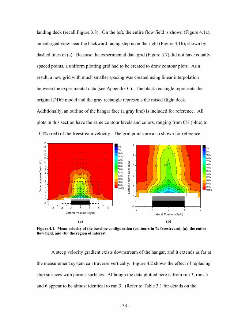
landing deck (recall Figure 3.8). On the left, the entire flow field is shown (Figure 4.1a);

an enlarged view near the backward facing step is on the right (Figure 4.1b), shown by

dashed lines in (a). Because the experimental data grid (Figure 3.7) did not have equally

spaced points, a uniform plotting grid had to be created to draw contour plots. As a

result, a new grid with much smaller spacing was created using linear interpolation

between the experimental data (see Appendix C). The black rectangle represents the

original DDG model and the gray rectangle represents the raised flight deck.

Additionally, an outline of the hangar face (a gray line) is included for reference. All

plots in this section have the same contour levels and colors, ranging from 0% (blue) to

104% (red) of the freestream velocity. The grid points are also shown for reference.

96%

88%

80%

72%

64%

56%48%

-3 -2 -1 0 1 2 3

-10123456789

101112131415

Lateral Position (2y/b)

Dis

tanc

e ab

ove

Dec

k (z

/h)

0%8%16%24%32%40%48%56%64%72%80%88%96%104%

96%

80%

72%

64%

56%

48%

-2 -1 0 1 2-1

0

1

2

3

4

5


Dis

tanc

e ab

ove

Dec

k (z

/h)

0%8%16%24%32%40%48%56%64%72%80%88%96%104%

(a) (b)

Figure 4.1. Mean velocity of the baseline configuration (contours in % freestream); (a), the entire flow field, and (b), the region of interest.

A steep velocity gradient exists downstream of the hangar, and it extends as far at

the measurement system can traverse vertically. Figure 4.2 shows the effect of replacing

ship surfaces with porous surfaces. Although the data plotted here is from run 3, runs 5

and 6 appear to be almost identical to run 3. (Refer to Table 3.1 for details on the

- 34 -

specific configurations of each run.) An easier comparison between configurations can

be made with velocity profile line plots, included in the next section. The mean velocity

gradient downstream of the hangar in run 3 is larger because the contour lines are closer

than for the baseline configuration. This phenomenon alone may increase workload for

the pilot, however, other factors, such as flow unsteadiness, must be considered. This is

discussed in detail in the remaining sections of this chapter.

80%

72%

80%

88%

88%

96%

96%

64%

56%

48%40%32%

24%

-2 -1 0 1 2-1

0

1

2

3

4

5


Dis

tanc

e ab

ove

Dec

k (z

/h)

0%8%16%24%32%40%48%56%64%72%80%88%96%104%

Figure 4.2. Run 3 mean velocity.

Figure 4.3 shows the mean velocity contours of run 8. This configuration

included injection from the hangar face. The mass flow rate was four cubic feet per

minute which translates to an injection velocity of 1.9 feet per second or 2.5% of the

freestream velocity. This configuration caused another increase in the mean velocity

gradient. The other two configurations which incorporated blowing (runs 7 and 9) have

mean velocity contours that do not differ as significantly with respect to the baseline.

- 35 -

80%

80% 88%

88%

96%

96%

72%

64%56%

48%

40% 32%24%

-2 -1 0 1 2-1

0

1

2

3

4

5


Dis

tanc

e ab

ove

Dec

k (z

/h)

0%8%16%24%32%40%48%56%64%72%80%88%96%104%


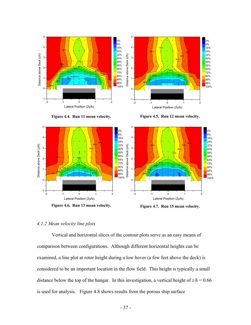
Next, consider the different fence configurations. Figure 4.4 shows the mean

velocity using the porous serrated fence. There is no longer a steep velocity gradient

downstream of the hangar. Instead, the velocity changes rapidly beyond the edge of the

fence. Figure 4.5 shows a slightly less severe gradient with the triangular-notched porous

fence (run 12). Runs 13 and 14 exhibit almost identical mean velocity contours. Because

the frontal areas of these fences are smaller, the gradient is not pushed as far away from

the hangar (see Figure 4.6). Finally, Figure 4.7 shows the mean velocity contours using

the reticulated foam fence (run 15). This configuration has similar results with runs 11

and 12, however, run 15 produced the largest region of low speed flow downstream of

the hangar.

- 36 -

80%

72%

80%

64%

88%

88%

96%

96%

56%

48%

40%

32%

24%24%


80%

80%

88%

88%

96%

96%

72%

64%

56% 48%

40%

32% 24%

-2 -1 0 1 2-1

0

1

2

3

4

5


Dis

tanc

e ab

ove

Dec

k (z

/h)

0%8%16%24%32%40%48%56%64%72%80%88%96%104%


80%

80%

88%

88%96%

96%

72%

64%

56%48%

40%32%

24%


80%

72%

80%

88% 88%

96%

96%

64%

56%

48%40%32%

24%

-2 -1 0 1 2-1

0

1

2

3

4

5


Dis

tanc

e ab

ove

Dec

k (z

/h)

0%8%16%24%32%40%48%56%64%72%80%88%96%104%


-2 -1 0 1 2-1

0

1

2

3

4

5


Dis

tanc

e ab

ove

Dec

k (z

/h)

0%8%16%24%32%40%48%56%64%72%80%88%96%104%

-2 -1 0 1 2-1

0

1

2

3

4

5


Dis

tanc

e ab

ove

Dec

k (z

/h)

0%8%16%24%32%40%48%56%64%72%80%88%96%104%

4.1.2 Mean velocity line plots

Vertical and horizontal slices of the contour plots serve as an easy means of

comparison between configurations. Although different horizontal heights can be

examined, a line plot at rotor height during a low hover (a few feet above the deck) is

considered to be an important location in the flow field. This height is typically a small

distance below the top of the hangar. In this investigation, a vertical height of z/h = 0.66

is used for analysis. Figure 4.8 shows results from the porous ship surface

- 37 -

configurations. The use of porous ship surfaces causes a decrease in the mean flow

across the flight deck. This may be a desirable effect since landing at higher velocity

means that a helicopter must be pitched downward to maintain a stationary position with

respect to the ship. Alternatively, this can be considered a negative effect if increased

hover performance is required. With an increased oncoming velocity, a helicopter may

be able to take off at higher gross weights. However, due to the limitations of the single

component hotwire, the mean velocities plotted here could come from any direction in

the vertical/longitudinal plane. The asymmetric feature in run 7 (shown in Figure 4.8)

results from a non-uniform injection velocity across the flight deck surface. Recall that

the circular baffle did not distribute the airflow uniformly.

The mean velocities for the fence configurations are shown in Figure 4.9. These

configurations show a larger decrease in mean velocity than the porous surface

configurations. The reticulated foam fence configuration (run 15) shows the lowest mean

velocity across the flight deck. However, there is a tradeoff with this improvement; a

steeper velocity gradient exists beyond the lateral edges of the ship (from |2y/b| = 1 to

|2y/b| = 1.5). As a result, if the pilot deviates laterally from an approach, he/she will be

caught in a steeper gradient than occurs for the baseline configuration.

- 38 -

0%

10%

20%

30%

40%

50%

60%

70%

80%

90%

100%

-1.5 -1.0 -0.5 0.0 0.5 1.0 1.5

Spanwise Position ( y/(b/2) )

Mea

n Ve

loci

ty (%

U in

f)

Run 2 (baseline)Run 3Run 5Run 6Run 7Run 8Run 9

Width of ship

Figure 4.8. Mean velocity at low hover (z/h = 0.66) for porous surface configurations

0%

10%

20%

30%

40%

50%

60%

70%

80%

90%

100%

-2.0 -1.5 -1.0 -0.5 0.0 0.5 1.0 1.5 2.0


Mea

n Ve

loci

ty (%

U in

f )

Run 2 (baseline)Run 11Run 12Run 13Run 14Run 15

Width of ship

Figure 4.9. Mean velocity at low hover (z/h = 0.66) for fence configurations.

- 39 -

0

0.5

1

1.5

2

2.5

0% 10% 20% 30% 40% 50% 60% 70% 80% 90% 100%

Mean Velocity (% Uinf)

Hei

ght (

# of

han

ger h

eigh

ts)


Top of hanger

Figure 4.10. Mean velocity on the vertical centerline (2y/b = 0) for porous surface configurations.

A vertical cut of the mean velocity contour plots also helps show quantitative

differences between configurations. Figure 4.10 plots the mean velocity at various

heights above the deck. Although there is little variance in the shape of these lines, most

configurations cause a slight increase in velocity. Recall from above that these

configurations tend to increase the velocity gradient behind the hangar, an undesirable

feature. The fence configurations produce a very different effect on the mean velocity

and are shown in Figure 4.11. Fences “shield” the flight deck. The serrated fence (run

11) has the most dramatic effect, keeping the velocity around 30% of freestream until

about 1.5 hangar heights. The other configurations have a similar effect, but do not keep

the mean velocity as low at heights above the top of the hangar. However, these other

configurations do have lower mean velocity near the flight deck compared with the

porous surface configurations.

- 40 -

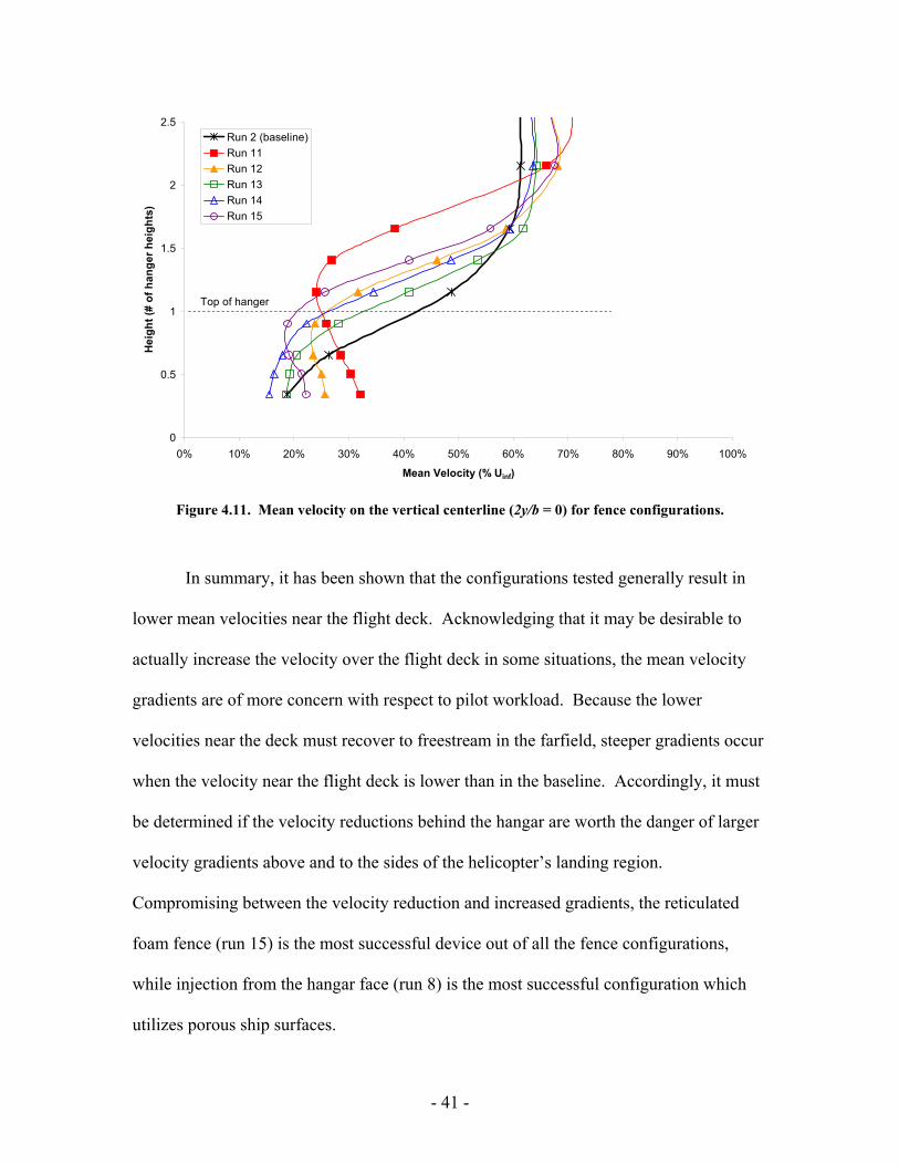
0

0.5

1

1.5

2

2.5

0% 10% 20% 30% 40% 50% 60% 70% 80% 90% 100%


Hei

ght (

# of

han

ger h

eigh

ts)


Top of hanger

Figure 4.11. Mean velocity on the vertical centerline (2y/b = 0) for fence configurations.

In summary, it has been shown that the configurations tested generally result in

lower mean velocities near the flight deck. Acknowledging that it may be desirable to

actually increase the velocity over the flight deck in some situations, the mean velocity

gradients are of more concern with respect to pilot workload. Because the lower

velocities near the deck must recover to freestream in the farfield, steeper gradients occur

when the velocity near the flight deck is lower than in the baseline. Accordingly, it must

be determined if the velocity reductions behind the hangar are worth the danger of larger

velocity gradients above and to the sides of the helicopter’s landing region.

Compromising between the velocity reduction and increased gradients, the reticulated

foam fence (run 15) is the most successful device out of all the fence configurations,

while injection from the hangar face (run 8) is the most successful configuration which

utilizes porous ship surfaces.

- 41 -

4.2 Velocity standard deviation

Although the mean flow variation over the landing deck provides a basic

understanding of the varying behaviors of different control techniques, it does not

provide information about the unsteadiness of the flow field. Since random fluctuations

are correlated with increased pilot workload,23 a measure of unsteadiness should be

calculated to determine the effectiveness of flow control devices. Consequently, the

standard deviation of the velocity time history at each grid point is computed. Although

mean velocity gradients can be a contributing cause to pilot workload, the unsteadiness in

the flow field is used as the primary metric for evaluation. For small fluctuations,

standard deviation, σ, is the RMS of the velocity fluctuations in the direction of the

measured resultant velocity. Recall that because a single component hotwire probe is

used, only the resultant of the freestream and vertical components is measured. A more

thorough discussion is available in Appendix A and B.

The contour plots that follow include all the configurations tested. The

unsteadiness from different configurations varies more from the baseline than the mean

velocity. The contours show the location of the greatest unsteadiness in the flow field

and provide insight on how to further decrease unsteadiness. Recall from the uncertainty

analysis that the measured velocity standard deviation in regions of high turbulence

intensity (typically below one hangar height) should be analyzed qualitatively only.

4.2.1 Velocity standard deviation contours

Perhaps the easiest way to get a general idea of how each flow control technique

performs is to examine contour plots of the velocity standard deviation at each grid point.

- 42 -

The baseline configuration is shown in Figure 4.12. The left plot shows the entire flow

field, and the area of interest is enlarged on the right. Again, the black rectangle

represents the original model, the gray rectangle represents the raised flight deck, and the

outline of the hangar face is represented by a gray line. The hotwire grid points are also

shown for reference. All plots have the same contour levels and colors, ranging from 0%

(blue) to 22% (red) of the freestream velocity.

-3 -2 -1 0 1 2 3

-10123456789

101112131415


Dis

tanc

e ab

ove

Dec

k (z

/h)

0%2%4%6%8%10%12%14%16%18%20%22%

-2 -1 0 1 2-1

0

1

2

3

4

5


Dis

tanc

e ab

ove

Dec

k (z

/h)

0%2%4%6%8%10%12%14%16%18%20%22%

(a) (b)

Figure 4.12. Velocity standard deviation of the baseline data; (a), the entire flow field, and (b), the region of interest.

Figures 4.13 and 4.14 show the contour plots which compare the effect of

“venting” the raised flight deck and hangar extension. Figure 4.13 is vented while Figure

4.14 is not. Both of these configurations show a slight reduction in maximum standard

deviation compared to the baseline. Upon closer inspection, it is seen that the non-vented

case has slightly less unsteadiness. As a result, the remainder of the porous surface

configurations did not incorporate venting; the sides of the raised flight deck and hangar

extension are solid. The effect of hole diameter is determined in Figure 4.15. The holes

- 43 -

in the porous surfaces in this configuration are 0.024 inches in diameter, as opposed to

0.0625 inches in the prior runs. Both materials had 23% open area. Little change occurs,

but a possible explanation is due to the vertical limit on the probe/traverse.

Measurements were only possible down to a height of 11/32 inch above the flight deck

surface, and it is likely that greater differences occur within this region. Regardless, it

was decided to move forward with the investigation using the material with smaller holes.

8%

8%

6%

6%

4%4%

2%

2%

10%

12% 14%

Figure 4.13. Velocity standard deviation of vented porous surface configuration (0.0625” holes, run 3).

8%

6%

6%

4%4%

2%

2% 10%

12% 14%

-2 -1 0 1 2-1

0

1

2

3

4

5


Dis

tanc

e ab

ove

Dec

k (z

/h)

0%2%4%6%8%10%12%14%16%18%20%22%

Figure 4.14. Velocity standard deviation of non-vented porous surface configuration (0.0625” holes, run 5).

8%

6%

6%

4%

4%

2%

2%

10%

12%14%

-2 -1 0 1 2-1

0

1

2

3

4

5


Dis

tanc

e ab

ove

Dec

k (z

/h)

0%2%4%6%8%10%12%14%16%18%20%22%

Figure 4.15. Velocity standard deviation of non-vented porous surface configuration (0.024” holes, run 6).

-2 -1 0 1 2-1

0

1

2

3

4

5


Dis

tanc

e ab

ove

Dec

k (z

/h)

0%2%4%6%8%10%12%14%16%18%20%22%

- 44 -

The main reason for this is because if the holes were scaled up to the actual size of the

ship, the smaller holes would be much more practical; a model scale of 0.024 inches

scales up to 3.46 inches in full scale.

Injection was then added to the model with porous surfaces. Figure 4.16 shows

run 7, which uses the circular baffle. Mass flow was 4 cubic feet per minute which

would ideally result in a uniform injection velocity of less than 1% of the freestream.

However, flow visualization showed that the injection uniformity is poor. Comparing

Figure 4.16 to 4.15, this type of injection has increased the areas of maximum standard

deviation. The next active technique was to inject through the porous hangar face in the

freestream direction. Mass flow was set to 4 cubic feet per minute, the highest obtainable

with the equipment available. By reducing the area of the surface injection, the new

injection velocity is 2.5% of the freestream. Because the injected air was deflected by

using a flat plate, there is still no assurance of uniform injection across the hangar face.

However, flow visualization showed a reasonably smooth, symmetric distribution across

the hangar face. Figure 4.17 shows the velocity standard deviation for this configuration.

Unsteadiness is decreased more with this configuration than with all others. Further

improvements are expected as the injection velocity is increased. Unfortunately, due to

hardware limitations, higher velocities could not be tested. Finally, run 9 was conducted

to determine if the improvements in run 8 could be obtained without using a porous flight

deck. Figure 4.18 shows the corresponding plot. In addition to the asymmetric feature,

the source of which is unknown, the flow field is more unsteady than for the prior case

(run 8). As a result, it is concluded that the reduction in unsteadiness in run 8 is caused

by a combination of both the porous flight deck and the injection from the hangar face.

- 45 -

By analysis of the contour plots, this configuration (run 8) causes the greatest reduction

in unsteadiness of all the porous surface techniques tested during this investigation.

8%

8%

6%

6%

4%

4%2%

2%

10%

12%

14% 14%

Figure 4.16. Velocity standard deviation of run 7 (injection using circular baffle).

8%

8%

6%

6%

4%

4%2%

2%

10%

12%

14%

14%

-2 -1 0 1 2-1

0

1

2

3

4

5

Lateral Position (2y/b)D

ista

nce

abov

e D

eck

(z/h

)

0%2%4%6%8%10%12%14%16%18%20%22%

Figure 4.17. Velocity standard deviation of run 8 (injection from hangar face).

8%

10%

8%

6%

6%

4%4%

2%

2%

12%

14%

-2 -1 0 1 2-1

0

1

2

3

4

5


Dis

tanc

e ab

ove

Dec

k (z

/h)

0%2%4%6%8%10%12%14%16%18%20%22%

Figure 4.18. Velocity standard deviation of run 9.

-2 -1 0 1 2-1

0

1

2

3

4

5


Dis

tanc

e ab

ove

Dec

k (z

/h)

0%2%4%6%8%10%12%14%16%18%20%22%

The second portion of the investigation explores the effects of fence

configurations. Figures 4.19 and 4.20 show the velocity standard deviation measured

with a ½ inch serrated porous fence (run 11) and a ½ inch triangular-notched porous

fence (run 12), respectively. Note that the height of the hangar is 1 inch on the model.

Because of their frontal area, fences tend to push the unsteady shear layer upward and

- 46 -

outward. Although this results in a region of increased unsteadiness directly downstream

of the fence edge, the unsteadiness inside the edges and downstream of the hangar is

significantly reduced. The serrated fence has a more turbulent shear layer, as the

triangular notches do not cause peaks in unsteadiness to be as large. Both configurations,

however, result in much lower unsteadiness downstream of the hangar face.

8%

10%

12%

14%

16%

10%

8%

6%

6%

10%4%

4%

2%2%

16%

14%12%

18%

Figure 4.19. Velocity standard deviation of the serrated porous fence configuration (run 11).

8%

10%

10%

12%

8%

6%

6%

4%

4%2%

2%

14%

12%

16%

-2 -1 0 1 2-1

0

1

2

3

4

5


Dis

tanc

e ab

ove

Dec

k (z

/h)

0%2%4%6%8%10%12%14%16%18%20%22%

Figure 4.20. Velocity standard deviation of the triangular-notched porous fence configuration (run12).

-2 -1 0 1 2-1

0

1

2

3

4

5


Dis

tanc

e ab

ove

Dec

k (z

/h)

0%2%4%6%8%10%12%14%16%18%20%22%

The next two figures show the flow field effects of the “mini delta wings”. Figure

4.21 shows run 13 which was constructed from porous sheet metal. The results show

decreased unsteadiness downstream of the fence edge, but the device no longer shields

the flight deck like the prior two fences did. Because the device was porous, a solid

version was also constructed to promote better formation of the small leading-edge

vortices. Figure 4.22 shows the resulting contour plot. Unfortunately, improvements

were not discovered. The asymmetries of the flow field may be caused by imperfections

in the fabrication process.

- 47 -

The final fence configuration tested was constructed of reticulated foam. Figure

4.23 shows the contour plot. This device is superior to the other fences for two reasons.

First, it does not have as much unsteadiness downstream of the fence edge as runs 11 and

12. Most importantly, however, this configuration actually shields the area behind the

hangar most effectively, resulting in the lowest amount of unsteadiness. In conclusion,

the reticulated foam fence performs the best.

8%

8%

6%

6%

4%

4%

2%

2%

10%

12%

14% 16%

Figure 4.21. Velocity standard deviation of porous “mini delta wing” configuration (run 13).

8%

10%

10%

8%

6%

6%

4%4% 2%

2%

12%

14%

16%

-2 -1 0 1 2-1

0

1

2

3

4

5


Dis

tanc

e ab

ove

Dec

k (z

/h)

0%2%4%6%8%10%12%14%16%18%20%22%

Figure 4.22. Velocity standard deviation of solid “mini delta wing” configuration (run 14).

8%

10% 10%

12%

14%

8%

6%

6%4%

4%

2%

2%

14%

12%

16%

10%

10%

-2 -1 0 1 2-1

0

1

2

3

4

5


Dis

tanc

e ab

ove

Dec

k (z

/h)

0%2%4%6%8%10%12%14%16%18%20%22%

Figure 4.23. Velocity standard deviation of reticulated foam fence configuration (run 15).

-2 -1 0 1 2-1

0

1

2

3

4

5


Dis

tanc

e ab

ove

Dec

k (z

/h)

0%2%4%6%8%10%12%14%16%18%20%22%

- 48 -

4.2.2 Velocity standard deviation line plots

As in the case of the mean velocity contour plots, the standard deviation contour

plots can be understood further by creating line plots. Figures 4.24 and 4.25 show the

standard deviation at a height corresponding to the rotor height at low hover. As

mentioned before, this height is z/h = 0.66. All of the configurations show an

improvement over the flight deck (|2y/b| < 1) compared to the baseline. Consistent with

the other plots, the configuration tested in run 8 leads to the greatest improvement. The

fence configurations produce large peaks outside the width of the ship, but allow for

substantial reductions in unsteadiness behind the hangar. The reticulated foam fence (run

15) causes the greatest reduction in unsteadiness.

Figures 4.26 and 4.27 show the standard deviation along the vertical centerline of

the measurement plane. The same trends are observed here. The porous surface and

blowing configurations (runs 3 to 9) generally decrease unsteadiness along the entire

centerline, and the fence configurations (runs 11 to 15) increase and shift the peak

standard deviation further above the flight deck.

- 49 -

0%

2%

4%

6%

8%

10%

12%

14%

16%

18%

20%

-1.5 -1.0 -0.5 0.0 0.5 1.0 1.5


Stan

dard

Dev

iatio

n (%

U in

f)


Width of ship

Figure 4.24. Velocity standard deviation at low hover for porous surface configurations.

0%

2%

4%

6%

8%

10%

12%

14%

16%

18%

20%

-2.0 -1.5 -1.0 -0.5 0.0 0.5 1.0 1.5 2.0


Stan

dard

Dev

iatio

n (%

U in

f)


Width of ship

Figure 4.25. Velocity standard deviation at low hover for fence configurations.

- 50 -

0

0.5

1

1.5

2

2.5

0% 2% 4% 6% 8% 10% 12% 14% 16% 18% 20%

Standard Deviation (% Uinf)

Hei

ght (

z/h)


Top of hanger

Figure 4.26. Velocity standard deviation along vertical centerline for porous surface configurations.

0

0.5

1

1.5

2

2.5

0% 2% 4% 6% 8% 10% 12% 14% 16% 18% 20%


Hei

ght (

z/h)


Top of hanger

Figure 4.27. Velocity standard deviation along vertical centerline for fence configurations.

- 51 -

4.3 Turbulence intensity

Turbulence intensity is defined as:

localUTI σ

=

which is the standard deviation divided by the total local mean velocity. This parameter

is often important in unsteady aerodynamic investigations; however its relevance to this

application is questionable. In ship airwake flow fields, the range of local velocities in

the vicinity of the flight deck can vary by almost an order of magnitude. Recalling

Figure 4.1, the mean velocity decreases to the 20% range of freestream velocity behind

the hangar. Because this parameter is in the denominator of the turbulence intensity

calculation, TI can become large very quickly. In addition, this application typically

causes the standard deviation to increase as the mean velocity decreases. As a result, it

becomes difficult to determine the effect of each flow control device. The following

discussion shows the difficulty in evaluating the flow control devices with this parameter

alone. Recall from the uncertainty analysis that regions of high turbulence intensity

(above 20% measured, typically below one hangar height) should be analyzed

qualitatively only.

4.3.1 Turbulence intensity contour plots

Figure 4.28 shows the turbulence intensity for the baseline configuration. Again,

all the plots in this section have the same contour levels and colors, ranging from 0%

(blue) to 65% (red) turbulence intensity. The baseline configuration has a radial contour

pattern and a maximum intensity of 50 to 55%. By comparing this figure with the

- 52 -

baseline mean velocity and standard deviation contours (Figures 4.1 and 4.12), one can

see that the shape of the turbulence intensity is driven by the mean velocity, not the

standard deviation. It is for this reason that turbulence intensity is not a robust parameter

for evaluation of flow control devices. Figures 4.29 and 4.30 show contours for the

porous surface configurations. The first presents the results from run 3 and is almost

identical to all the passive porous surface configurations. Figure 4.30 shows slightly

higher maximum turbulence intensities for run 8 when compared with the other porous

surface configurations. Like the baseline, however, these contours are shaped from the

mean velocity. The differences between the configurations shown by the standard

deviation are simply not visible here.

10%

5%

5%

15%

20%

25%30%

35%

40%45% 50%

-2 -1 0 1 2-1

0

1

2

3

4

5


Dis

tanc

e ab

ove

Dec

k (z

/h)

0%5%10%15%20%25%30%35%40%45%50%55%60%65%

Figure 4.28. Turbulence intensity of the baseline configuration.

- 53 -

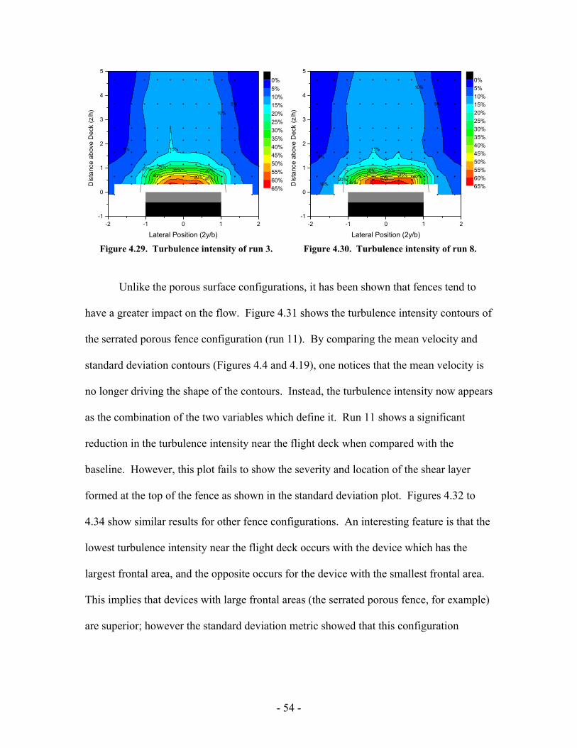
10%

10%

5%

5% 15%

20% 25%30%35%

40% 45%50%

Figure 4.29. Turbulence intensity of run 3.

10%

10%

5%

5%

15%

20%

25%30%

35%40%45%50%

55%

-2 -1 0 1 2-1

0

1

2

3

4

5


Dis

tanc

e ab

ove

Dec

k (z

/h)

0%5%10%15%20%25%30%35%40%45%50%55%60%65%


-2 -1 0 1 2-1

0

1

2

3

4

5


Dis

tanc

e ab

ove

Dec

k (z

/h)

0%5%10%15%20%25%30%35%40%45%50%55%60%65%

Unlike the porous surface configurations, it has been shown that fences tend to

have a greater impact on the flow. Figure 4.31 shows the turbulence intensity contours of

the serrated porous fence configuration (run 11). By comparing the mean velocity and

standard deviation contours (Figures 4.4 and 4.19), one notices that the mean velocity is

no longer driving the shape of the contours. Instead, the turbulence intensity now appears

as the combination of the two variables which define it. Run 11 shows a significant

reduction in the turbulence intensity near the flight deck when compared with the

baseline. However, this plot fails to show the severity and location of the shear layer

formed at the top of the fence as shown in the standard deviation plot. Figures 4.32 to

4.34 show similar results for other fence configurations. An interesting feature is that the

lowest turbulence intensity near the flight deck occurs with the device which has the

largest frontal area, and the opposite occurs for the device with the smallest frontal area.

This implies that devices with large frontal areas (the serrated porous fence, for example)

are superior; however the standard deviation metric showed that this configuration

- 54 -

produced the largest peaks in unsteadiness. Thus, the turbulence intensity metric appears

to be unable to evaluate control devices accurately.

10%

15%20%

25%

30%

10%

5%

5%

35%

40%

45%

50%


10%

15%

10% 5%

5% 20%

25%

30%35%

40%

45%

50%

-2 -1 0 1 2-1

0

1

2

3

4

5

Lateral Position (2y/b)D

ista

nce

abov

e D

eck

(z/h

)

0%5%10%15%20%25%30%35%40%45%50%55%60%65%


10%

10%

5%

5%

15%

20% 25%

30%

35%40%

45%

50%


-2 -1 0 1 2-1

0

1

2

3

4

5


Dis

tanc

e ab

ove

Dec

k (z

/h)

0%5%10%15%20%25%30%35%40%45%50%55%60%65%


-2 -1 0 1 2-1

0

1

2

3

4

5


Dis

tanc

e ab

ove

Dec

k (z

/h)

0%5%10%15%20%25%30%35%40%45%50%55%60%65%

-2 -1 0 1 2-1

0

1

2

3

4

5


Dis

tanc

e ab

ove

Dec

k (z

/h)

0%5%10%15%20%25%30%35%40%45%50%55%60%65%

4.3.2 Turbulence intensity line plots

Line plots of the turbulence intensity enable one to quantify the statements made

in the prior section. Figures 4.35 and 4.36 show the turbulence intensities corresponding

to a low hover height (z/h = 0.66). By visual inspection, it can be seen that for every

configuration, the average turbulence intensity across the flight deck is higher than the

- 55 -

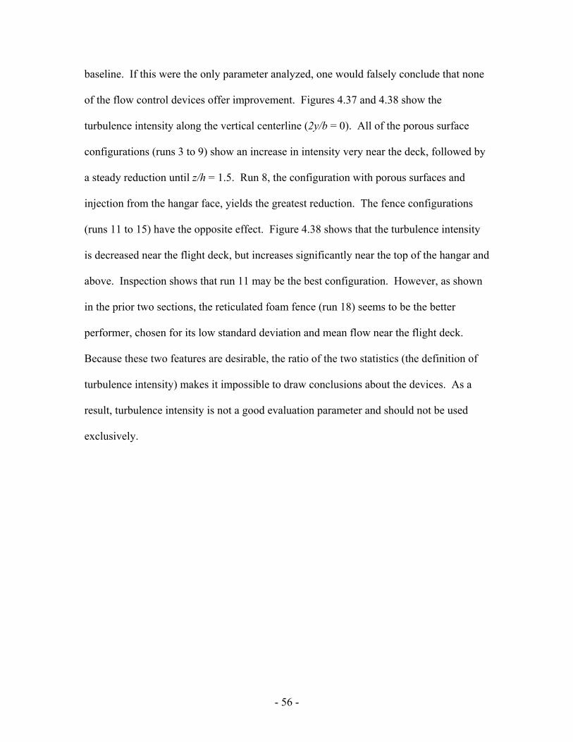
baseline. If this were the only parameter analyzed, one would falsely conclude that none

of the flow control devices offer improvement. Figures 4.37 and 4.38 show the

turbulence intensity along the vertical centerline (2y/b = 0). All of the porous surface

configurations (runs 3 to 9) show an increase in intensity very near the deck, followed by

a steady reduction until z/h = 1.5. Run 8, the configuration with porous surfaces and

injection from the hangar face, yields the greatest reduction. The fence configurations

(runs 11 to 15) have the opposite effect. Figure 4.38 shows that the turbulence intensity

is decreased near the flight deck, but increases significantly near the top of the hangar and

above. Inspection shows that run 11 may be the best configuration. However, as shown

in the prior two sections, the reticulated foam fence (run 18) seems to be the better

performer, chosen for its low standard deviation and mean flow near the flight deck.

Because these two features are desirable, the ratio of the two statistics (the definition of

turbulence intensity) makes it impossible to draw conclusions about the devices. As a

result, turbulence intensity is not a good evaluation parameter and should not be used

exclusively.

- 56 -

0

10

20

30

40

50

60

-1.5 -1.0 -0.5 0.0 0.5 1.0 1.5


Turb

ulen

ce In

tens

ity (%

)


Width of ship

Figure 4.35. Turbulence intensity at low hover (z/h = 0.66) for porous surface configurations.

0

10

20

30

40

50

60

-2.0 -1.5 -1.0 -0.5 0.0 0.5 1.0 1.5 2.0


Turb

ulen

ce In

tens

ity (%

)


Width of ship

Figure 4.36. Turbulence intensity at low hover (z/h = 0.66) for fence configurations.

- 57 -

0

0.5

1

1.5

2

2.5

0 10 20 30 40 50 60

Turbulence Intensity (%)

Hei

ght (

z/h)


Top of hanger

Figure 4.37. Turbulence intensity on the vertical centerline (2y/b = 0) for porous surface

configurations.

0

0.5

1

1.5

2

2.5

0 10 20 30 40 50 60


Hei

ght (

z/h)


Top of hanger

Figure 4.38. Turbulence intensity on the vertical centerline (2y/b = 0) for fence configurations.

- 58 -

4.4 Average unsteadiness in landing area

The prior sections in this chapter have concluded that the porous surface

configuration with injection from the hangar face (run 8) and the reticulated foam fence

(run 15) appear to be the superior techniques for reducing unsteadiness. It has been

shown that each offer their own advantages and disadvantages, but it is difficult to

determine which are important to a pilot. Consequently, the following metric is

considered.

Helicopter approaches to ships are flown on a specific path. For DDG class ships,

helicopters approach directly from the stern. Most pilots then come to a stop relative to

the ship and hover about 10 feet over the landing spot before descending to the deck.37

By considering this altitude and the height of a typical naval helicopter, the altitude of the

highest point on the helicopter can be calculated. Consequently, it is assumed that the

airwake above this height does not affect the handling qualities of the helicopter. This is

a key assumption, and the method with which this height is chosen is important. To be

the most accurate, this height should be 1 to 2 rotor diameters above rotor height.

However, because others23 have shown that the unsteady fuselage loads can be correlated

with pilot workload, the airwake entrained by the rotor may be of lesser importance.

Therefore a lower height is acceptable, and it is first assumed to be a few feet above the

rotor. Similarly, spanwise limits can be placed on the airwake, outside which it is

assumed that there are again no effects on the helicopter. These limits are initially chosen

at the edges of the ship. Figure 4.39 shows how these constraints appear on the baseline

velocity standard deviation flow field. The upper limit is at z/h = 1.9.

- 59 -

-2 -1 0 1 2-1

0

1

2

3

4

5


Dis

tanc

e ab

ove

Dec

k (z

/h)

0%2%4%6%8%10%12%14%16%18%20%22%

Figure 4.39. Baseline velocity standard deviation. The box encloses the region in the airwake which affects helicopter operations.

With a fixed landing region in the flow field defined, the average unsteadiness can

be calculated by computing the mean of the standard deviation at every grid point in this

region. This is analogous to computing the volume under a three-dimensional contour

plot and dividing by the area of the data plane. Alternatively, calculating this average

using the variance instead of the standard deviation would provide a measurement of the

total kinetic energy in the flow in the landing region. However, because results presented

thus far have been based on standard deviation, the average unsteadiness metric is

calculated using the standard deviation. Noting that the experimental grid points in this

region are not equally spaced, a uniformly spaced grid must first be produced. Failing to

do so would result in weighting the values of closely spaced points more heavily. The

same linear interpolation used to create the contour plots is used to create a 900 point,

equally spaced grid. Finally, the values are averaged, resulting in a single number which

can be used for comparison between configurations.

- 60 -

Table 4.1 lists each configuration with the average unsteadiness parameter and the

corresponding percent change from the baseline configuration. Figure 4.40 shows a

visual comparison. The previous conclusions for the porous surface configurations (runs

3 to 9) are consistent with this new metric, and the improvements have now been

quantified with a single parameter. By using a porous flight deck and injection from the

hangar face (run 8), the unsteadiness is reduced 6.56%. The fence configurations,

however, all reveal an increase in unsteadiness. All of the fences tested had a height of

0.5h, which does not push the shear layer out of the landing region defined above.

Although the unsteadiness was significantly reduced behind the hangar, the current

metric also factors in the unsteadiness of this shear layer (occurring at a height around z/h

= 1.5). If the fence were two or three times higher, the shear layer would then be outside

of the defined landing region, and the average unsteadiness parameter would decrease.

By comparing runs 11 to 15 with each other, additional observations can be made. The

serrated porous fence (run 11) and the triangular-notched porous fence (run 12) cause a

considerable increase in unsteadiness in the landing region (14.99% and 13.04%

respectively). As a result, these configurations may not be the best option even if the size

of the fence, and hence the “sheltered” region, is increased. The remaining

configurations do not cause as significant increases in this investigation, so they should

perform better if their height is increased. Relative to the amount of frontal area of the

remaining fences, the reticulated foam fence (run 15) produces the least amount of

additional unsteadiness in the landing region. Therefore, it is recommended that future

investigations include a large (on the order of the height of the hangar) reticulated foam

fence.

- 61 -

Table 4.1. Average unsteadiness of each configuration.

Run # Configuration

Average unsteadiness

(standard deviation in %

freestream)

Percentchange

(%)

2 Baseline 12.49 - 3 Porous surfaces (0.0625” holes) with “venting” 12.20 -2.33 5 Porous surfaces (0.0625” holes) 12.08 -3.27 6 Porous surfaces (0.024” holes) 11.98 -4.07 7 Porous surfaces (0.024” holes) + injection using circular baffle 12.48 -0.06 8 Porous surfaces (0.024” holes) + injection from hangar face 11.67 -6.56

9 Porous surfaces (0.024” holes) + injection from hangar face (solid flight deck) 12.04 -3.66

11 Serrated porous fence 14.37 14.99 12 Triangular-notched porous fence 14.12 13.04 13 Triangular-notched porous fence angled 60 degrees upstream 13.48 7.94 14 Triangular-notched solid fence angled 60 degrees upstream 13.12 5.03 15 Reticulated foam fence 13.14 5.18

0.00%

-2.33

%

-3.27

%

-4.07

%

-6.56

%-3.

66%

14.99

%

13.04

%

7.94%

5.03%

5.18%

-0.06

%

-10%

-5%

0%

5%

10%

15%

20%

2 3 5 6 7 8 9 11 12 13 14 15

Run number

Perc

ent c

hang

e fr

om b

asel

ine

Figure 4.40. Percent change of the average unsteadiness in the landing region with respect to the baseline.

- 62 -

As mentioned previously, the landing region was defined using some specific

assumptions. As a result, it is of interest to determine the sensitivity of the landing region

dimensions. Because it may be difficult for a pilot to remain directly over the flight deck

while fighting the unsteady airwake, the landing region is expanded laterally. Figure 4.41

shows the two additional dimensions on the baseline flow field. The width has been

increased to |2y/b| = 1.4 and |2y/b| = 1.7. Similarly, Figure 4.42 shows changes to upper

limit of the landing region (z/h = 1.9, 2.4, and 2.9). The average unsteadiness is

calculated again for each configuration and landing region. Increasing the width (Figure

4.43) causes different effects for the two categories of flow control techniques. A wider

landing region causes the average unsteadiness for the porous surface configurations

(runs 3 to 9) to approach the baseline value (or 0% change on the chart). This occurs

because these configurations do not have any protrusions in the flow, and more portions

of the unaffected airwake are included in the average. On the other hand, fences have the

opposite effect since the outward shifted shear layer, caused by the fences on the sides of

the ship, is included when widening the landing region.

-2 -1 0 1 2-1

0

1

2

3

4

5


Dis

tanc

e ab

ove

Dec

k (z

/h)

0%2%4%6%8%10%12%14%16%18%20%22%

Figure 4.41. Width changes to the landing region ( |2y/b| = 1, 1.4, 1.7) overlaid on the velocity standard deviation contour plot.

Figure 4.42. Height changes to the landing region (z/h = 1.9, 2.4, 2.9) overlaid on the velocity standard deviation contour plot.

8%

6%

6%

4%4%

2%

2% 10%

12%14%

14%

-2 -1 0 1 2-1

0

1

2

3

4

5


Dis

tanc

e ab

ove

Dec

k (z

/h)

0%2%4%6%8%10%12%14%16%18%20%22%

- 63 -

Increasing the height of the landing region causes a similar behavior for the

porous surface configurations (Figure 4.44). Alternatively, because the top parts of the

fences were already included in the original landing region, these configurations (runs 11

to 15) decrease the effect on the airwake with height. The average unsteadiness again

begins to approach the baseline value. If a taller fence were used, one which pushes the

shear layer completely above the defined landing region, a decrease in the average

unsteadiness in this region would certainly occur. To achieve this requires a full-scale

fence at least 12 feet tall. A fence on this scale could be deployable so that it is raised

during helicopter/ship operations only.

-10%

-5%

0%

5%

10%

15%

20%

25%

30%

2 3 5 6 7 8 9 11 12 13 14 15

Run number

Perc

ent c

hang

e fr

om b

asel

ine

of a

vera

ge u

nste

adin

ess

Landing region => |2y/b| < 1Landing region => |2y/b| < 1.4Landing region => |2y/b| < 1.7

Figure 4.43. Bar graph showing the effect of widening the landing area.

- 64 -

-10%

-5%

0%

5%

10%

15%

20%

25%

30%

2 3 5 6 7 8 9 11 12 13 14 15

Run number

Perc

ent c

hang

e fr

om b

asel

ine

of a

vera

ge u

nste

adin

ess

Landing region => z/h < 1.9Landing region => z/h < 2.4Landing region => z/h < 2.9

Figure 4.44. Bar graph showing the effect of raising the height of landing area.

In summary, the average unsteadiness metric is useful because different flow

control devices can be compared quantitatively by a single parameter. One disadvantage

of the metric is that the flow outside the landing region is completely ignored. As a

result, a very large fence that completely shields the landing region is a solution.

Optimizing a device for this metric alone however, could lead to uncontrollable handling

qualities if a pilot were to stray out of the landing region.

4.5 Frequency analysis

Frequency analysis is used in fluid dynamics to identify evidence of periodic

shedding. If coherent structures can be identified in the flow, new flow control

techniques may be developed. Low speed flow over bluff bodies typically produces a

von Karman vortex street in the wake. This type of periodicity has also been observed in

- 65 -

flow visualization experiments on small naval vessels.11 Although characteristic

shedding can perform significantly differently at full scale, a spectral analysis provides

useful information about the behavior of the flow.

4.5.1 Calculation of frequency spectra

Generally speaking, frequency spectra are determined by calculating the discrete

Fourier transform (DFT) of each velocity time history. Recall that the sampling rate and

length is 4000 hertz for 4 seconds. As a result, information at frequencies up to 2000

hertz can be obtained without concerns of aliasing. On the other hand, the lowest

frequency that can be captured depends on the amount of data acquired. Since data is

collected over a four second interval, it can be assumed that frequencies as low as 0.25

hertz are resolved. This leads to a very noisy frequency spectrum from which it would be

difficult to extract useful information. One would need many samples of this length to

gain statistical confidence. To work around this problem, two approaches can be taken.

First, many shorter duration DFTs could be averaged together at the expense of low

frequency resolution, and second, the DFT could be passed through a low-pass digital

filter to remove noise. This investigation used both of these techniques. Although the

first is the preferred method, only a single 4-second time history was taken at each grid

point. To produce many DFTs to average together, the time history must be divided into

smaller segments. The consequence of this technique is a loss in frequency resolution.

As a result, the number of divisions of the 4-second time history is limited so that the loss

in resolution is minimized. However, the resulting DFT still contains more noise than

desired; therefore it was passed through a low-pass digital filter. Details about these

- 66 -

digital signal processing techniques are found in the literature.38 The MATLAB script

found in Appendix D was used to calculate the DFT and plot the power spectral density

(PSD). The y-axis in the PSD was scaled by the sampling frequency.

Each 4-second time history consists of 16,384 points. Prior to calculating a PSD,

the mean is subtracted from the time history so that the transform occurs only on the

unsteady fluctuations. The signal was then divided into 16 segments, each 1,024 points

in length. A PSD is calculated for each segment, and all are averaged together. This

results in a frequency resolution of approximately 4 hertz. In addition to the 16 unique

segments from the original time history, the averaged PSD also consists of 15 additional

segments created by overlapping neighboring segments by 50%. A schematic is shown

in Figure 4.45. Although these segments do not contain unique data, they do provide a

slight decrease in the amount of noise. Figure 4.46 is an example of how this averaging

technique removes noise in the PSD.

1024Segment

16,384 point time history

16 unique segments

15 overlapping segments

Figure 4.45. Diagram of how data was divided to produce the PSD.

- 67 -

Figure 4.46. Effect of averaging several individual PSDs.

Although the PSD has been significantly improved, the remaining noise still

makes it difficult to compare PSDs at different grid points. As a result, the PSD is passed

through a low-pass digital filter with a cut-off frequency at 15% of the sample rate. An

example of this smoothing effect is seen in Figure 4.47.

Figure 4.47. Effect of passing the PSD through a low-pass digital filter (smoothed).

- 68 -

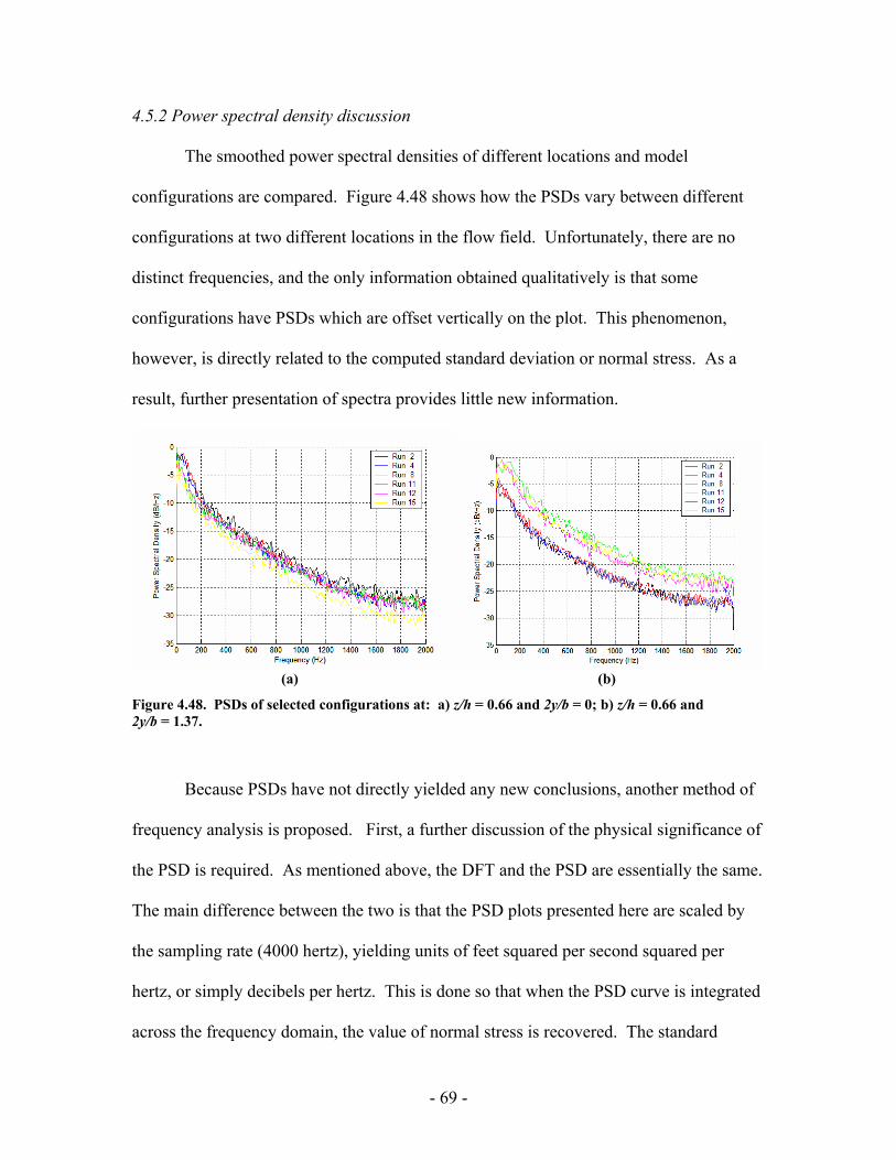
4.5.2 Power spectral density discussion

The smoothed power spectral densities of different locations and model

configurations are compared. Figure 4.48 shows how the PSDs vary between different

configurations at two different locations in the flow field. Unfortunately, there are no

distinct frequencies, and the only information obtained qualitatively is that some

configurations have PSDs which are offset vertically on the plot. This phenomenon,

however, is directly related to the computed standard deviation or normal stress. As a

result, further presentation of spectra provides little new information.

(a) (b)

Figure 4.48. PSDs of selected configurations at: a) z/h = 0.66 and 2y/b = 0; b) z/h = 0.66 and 2y/b = 1.37.

Because PSDs have not directly yielded any new conclusions, another method of

frequency analysis is proposed. First, a further discussion of the physical significance of

the PSD is required. As mentioned above, the DFT and the PSD are essentially the same.

The main difference between the two is that the PSD plots presented here are scaled by

the sampling rate (4000 hertz), yielding units of feet squared per second squared per

hertz, or simply decibels per hertz. This is done so that when the PSD curve is integrated

across the frequency domain, the value of normal stress is recovered. The standard

- 69 -

deviation is then simply the square root of this quantity. The PSDs also show that the

majority of the energy in the flow originates in the lower frequencies. This low

frequency region is important since these fluctuations cause excess pilot workload. As a

result, the integration of the PSD up to a certain frequency will allow a numerical

comparison of these low frequency fluctuations. Likewise, the unsteady fluctuations in

the high frequency domain are also examined.

The frequency defining the difference in low and high frequencies is called the

cut-off frequency. Determination of this parameter is difficult and several methods are

proposed. First, the frequency which divides the PSD into approximately equal areas can

be chosen. Another method involves using the characteristic shedding frequency of the

model (even though this shedding is not observed). A third method involves the physics

of turbulence. All three of these methods are considered.

The first method yields an even breakdown of energy. Because there are no

distinct frequencies, the PSD could be split into two equal areas with the dividing line

being the cut-off frequency. This avoids the defined low frequency unsteadiness

becoming similar in magnitude to the total unsteadiness. The second method requires

consideration of bluff body aerodynamics. Given the Reynolds number of the

experiment, the Strouhal number is approximated. However, because the Reynolds

number is near the supercritical regime, periodic shedding is not achieved.39 This is a

possible explanation for the lack of detection of large coherent structures, and hence a

dominant frequency. The third method considers the physics of turbulence. Figure 4.49

shows a typical frequency spectrum on a log-log scale. Turbulence consists of three

distinct regions in high Reynolds number flows.40 The first is the energy containing

- 70 -

region which consists of the lowest frequencies. Second, the inertial subrange exists at

moderate frequencies. This region is characterized by Kolmogorov’s hypothesis and

spectra which fall off at a rate proportional to frequency raised to the -5/3 power. Larger

eddies are broken up into smaller eddies by inertial effects. Third, the dissipation region

is where the smallest eddies are broken up due to viscous effects. This region cannot be

seen in the data due to the limited sampling frequency. Considering these three spectrum

ranges, a logical cut-off would be at the transition to the inertial subrange because it is

desired to isolate the low, energy-containing frequencies.

Energy-containing range Inertial subrange Dissipation range

Figure 4.49. Velocity spectra following Kolmogorov’s hypothesis.

After considering these three methods, the cut-off frequency was chosen by a

combination of the first and third methods. Recall that the original time histories were

divided into segments of 1,024 samples, producing PSDs with a sensitivity of about 4

hertz. As a result, the cut-off frequency should be on the order of 100 hertz to integrate

- 71 -

over a reasonable number of points. Compromising between obtaining equal areas

beneath the PSD and using a sufficiently large number of points for the integration, a cut-

off frequency of 125 hertz was chosen. This is also near the beginning of the inertial

subrange as mentioned above.

The PSD from each grid point is numerically integrated to the cut-off frequency

(0 to 125 hertz); the trapezoidal method is used on the unfiltered PSD. The ratio of the

standard deviation at each grid point due to low frequencies to the total standard

deviation is shown in Figure 4.50. In the wake regions, the lower frequencies dominate

the turbulence, whereas the freestream is dominated by higher frequency turbulence.

-3 -2 -1 0 1 2 3-10123456789

101112131415


Dis

tanc

e ab

ove

Dec

k (z

/h)

0

0.1

0.2

0.3

0.4

0.5

0.6

0.7

0.8

0.9

1.0

Figure 4.50. Ratio of the standard deviation due to low frequencies to the total standard deviation for the baseline configuration.

4.5.3 Frequency-separated standard deviation contours

Contour plots similar to those in Section 4.2.1 are generated from the low and

high frequency standard deviation values. Figure 4.51 shows the baseline velocity

- 72 -

standard deviation in both the low and high frequency domains. Note that if the values at

each point on these two plots were summed, the standard deviation contours presented in

Section 4.2.1 would be recovered. The contour levels and colors are exactly the same as

those presented earlier, going from 0% (blue) to 22% (red) of the freestream. These two

plots serve as a new baseline for comparison between devices. The lower frequencies are

dominant, but increased high frequency fluctuations are present near the sides of the ship.

6%

4%

4%

2%

2%8%

10%

8%

2%

2%

4%4%

-2 -1 0 1 2-1

0

1

2

3

4

5


Dis

tanc

e ab

ove

Dec

k (z

/h)

0%2%4%6%8%10%12%14%16%18%20%22%

-2 -1 0 1 2

-1

0

1

2

3

4

5


Dis

tanc

e ab

ove

Dec

k (z

/h)

0%2%4%6%8%10%12%14%16%18%20%22%

(a) (b)

Figure 4.51. Baseline velocity standard deviation for: (a) the 0 – 125 Hz domain; (b) the 125 – 2000 Hz domain.

This frequency domain breakdown is consistent with the conclusions for the

porous surface configurations. Figure 4.52 shows the contours for the case with a porous

flight deck and injection from the hangar face (run 8). Other porous surface

configurations experience similar changes when separated into low and high frequencies.

Note again that an increase in high frequency unsteadiness occurs near the sides on the

hangar. The region of high frequency unsteadiness does not occur at the top of the

hangar in the middle because the oncoming flow has less energy. This is a result of the

lower mean velocity near the centerline of the ship due to the wake of upstream bodies

- 73 -

(the ship’s mast, bridge, stacks, etc.). Examining standard deviation contours of the fence

configurations verifies this statement. Figure 4.53 shows the serrated porous fence

configuration (run 11). The unsteady regions in this case are pushed upward and

outward, however, the high frequency unsteadiness is greater in areas with a higher mean

velocity. Other fence configurations exhibit similar characteristics.

6%

6%

4%

4%

2%

2%

8%

10%

8%

6%

2%

2%

4% 4%

-2 -1 0 1 2-1

0

1

2

3

4

5


Dis

tanc

e ab

ove

Dec

k (z

/h)

0%2%4%6%8%10%12%14%16%18%20%22%

-2 -1 0 1 2

-1

0

1

2

3

4

5


Dis

tanc

e ab

ove

Dec

k (z

/h)

0%

2%

4%

6%

8%

10%

12%

14%

16%

18%

20%

22%

(a) (b)

Figure 4.52. Velocity standard deviation for the porous flight deck with blowing from the hangar face for: (a) the 0 – 125 Hz domain; (b) the 125 – 2000 Hz domain.

6%

8%10%

6%4%

4%

2%

2%

10%

12%

14%

8%

8%

4%

2%

2%

-2 -1 0 1 2-1

0

1

2

3

4

5


Dis

tanc

e ab

ove

Dec

k (z

/h)

0%2%4%6%8%10%12%14%16%18%20%22%

-2 -1 0 1 2

-1

0

1

2

3

4

5


Dis

tanc

e ab

ove

Dec

k (z

/h)

0%2%4%6%8%10%12%14%16%18%20%22%

(a) (b)

Figure 4.53. Velocity standard deviation for the porous serrated fence configuration for: (a) the 0 – 125 Hz domain; (b) the 125 – 2000 Hz domain.

- 74 -

4.5.4 Alternative frequency breakdown

Another method to determine the cut-off frequency is to consider the frequency

scaling between full scale and the wind tunnel tests. A model scale of 1:144 multiplies

by a velocity scale of approximately 1:1.5 yielding a frequency scaling of 216:1. Also

note that frequencies between 0.1 and 2 hertz are responsible for increased pilot

workload.33 Therefore, this method implies the frequency domain of interest in this

investigation is 21.6 to 432 hertz. The unsteadiness now responsible for pilot workload

can be obtained by integrating the PSD over these frequencies. Unfortunately because

the McRuer33 paper was discovered after analysis was completed, this new frequency

range was unable to be completed for inclusion in this document. However, because this

method includes much of the energy containing region, it is expected that it will produce

contours similar to the low frequency contours shown above.

4.5.5 Frequency analysis summary

Conclusions of the frequency analysis are summarized. First, the power spectral

densities of velocity time histories do not reveal any dominate frequencies. The only

difference between configurations is that more unsteadiness causes the y-intercept of the

PSD to increase. Second, the spectra are used to separate the low frequency unsteadiness

from the high frequency unsteadiness by selecting a cut-off frequency. Upon replotting

the contours in Section 4.2.1, conclusions regarding the performance of control devices

were not changed. Finally, these contours show that high frequency unsteadiness is more

common in regions of higher mean velocity. This implies that the fence configurations

successfully break up some of the larger flow structures and shift them into the higher

- 75 -

frequency domain, but only in regions of higher mean velocity near the sides of the ship.

As a result, a future investigation should include configurations with flow control devices

(fences for example) on the sides of the hangar only.

- 76 -

5. RESULTS AND DISCUSSION: 20 DEGREES

WIND-OVER-DECK

Because ships rarely cruise directly into a headwind, nonzero wind-over-deck

(WOD) angles must be considered. The focus of the investigation was to evaluate

several flow control devices to determine which was most effective in decreasing pilot

workload. It was desired to test a wide range of devices rather than focus on the effects

of varying the WOD angle. As a result, only two flow control devices were chosen for

evaluation at 20 degrees WOD. The best performing devices from each category in

Chapter 4 were the configuration with porous ship surfaces and injection from the hangar

face (run 8) and the reticulated foam fence configuration (run 15). Note that the model

was rotated about the stern in the wind tunnel, but the measurement system and traverse

remained orthogonal to the tunnel. Consequently, the data plane was skewed with

respect to the flight deck; however, the axial position of the measurement plane still

passed through the middle of the flight deck. Because of this skewness, the contour plots

at this WOD angle include a ship cross-section that is slightly wider than the 0 degrees

WOD case (the same non-dimensionalization parameters are used). Recall from the

uncertainty analysis that the measurements in regions of high turbulence intensity should

be analyzed qualitatively only. Because the ship is yawed 20 degrees, this region is much

larger than for the 0 degrees WOD case.

- 77 -

5.1 Mean velocity

5.1.1 Mean velocity contours

Consider the baseline mean velocity contour plot for the 20 degrees WOD case

shown in Figure 5.1. Because the hangar face is upstream of the data plane, its projection

is offset to the right as shown in the figure. The contour levels and colors are the same as

in Section 4.1.1 ranging from 0% (blue) to 104% (red) of the freestream velocity. The

large velocity deficit on the right side of the figure is caused by the mast, antennas,

stacks, etc. Interestingly, the lowest mean velocity is measured on the windward side of

the side of the flight deck.

-1 0 1 2

88%

80%96%

72%

64%

56%

48%

40%32%

-1

0

1

2

3

4

5

Dis

tanc

e ab

ove

Dec

k (z

/h)

0%8%16%24%32%40%48%56%64%72%80%88%96%104%


Figure 5.1. Mean velocity for the 20 degrees WOD baseline configuration. The contours are in percent of freestream velocity.

The mean velocity contours of the two flow control devices tested at this WOD

angle are shown in Figures 5.2 and 5.3. The reticulated foam fence (run 17) has caused a

much larger region of low speed flow behind the hangar. Unfortunately, the velocity

gradients have also become much larger, especially on the windward side of the ship.

- 78 -

The fence on the leeward side appears to have little effect on the mean as the flow on the

starboard side of the ship already has a massive velocity deficit. The other configuration

(run 18) shows a flow field more similar to the baseline, however the velocity behind the

hangar has decreased.

-1 0 1 2

88%

80%

72%

96%

64%56%

48%

40%

32%

24%

16%

Figure 5.2. Mean velocity of reticulated foam fence configuration (run 17).

-1 0 1 2

88%

80%

96%

72%

64%

56%48%40%32%

24%

-1

0

1

2

3

4

5

Dis

tanc

e ab

ove

Dec

k (z

/h)

0%8%16%24%32%40%48%56%64%72%80%88%96%104%

Lateral Position (2y/b) Figure 5.3. Mean velocity of porous surfaces with injection configuration (run 18).

-1

0

1

2

3

4

5

Dis

tanc

e ab

ove

Dec

k (z

/h)

0%8%16%24%32%40%48%56%64%72%80%88%96%104%


5.1.2 Mean velocity line plots

The features observed in the contour plots are better quantified by examining line

plots of data in the measurement plane. Figures 5.4 and 5.5 show a horizontal and

vertical slice of data. The location of the horizontal slice is the same height of those in

the prior chapter. This height (z/h = 0.66) corresponds to rotor height at a hover a few

feet above the deck. The vertical cut was taken at 2y/b = 0.23. This slightly off-center

coordinate was chosen because of the nonzero WOD angle. The data shows that the

foam fence causes the mean velocity to decrease by a factor of three at many spanwise

locations across the flight deck. The downside is the very steep gradient on the windward

side of the ship. Although this feature is not located over the center of the flight deck at

20 degrees WOD, the steep velocity gradient is likely to move towards the leeward side

- 79 -

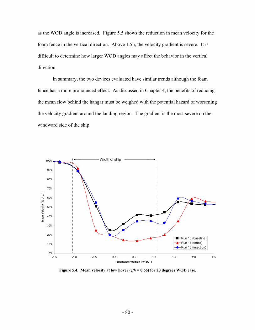
as the WOD angle is increased. Figure 5.5 shows the reduction in mean velocity for the

foam fence in the vertical direction. Above 1.5h, the velocity gradient is severe. It is

difficult to determine how larger WOD angles may affect the behavior in the vertical

direction.

In summary, the two devices evaluated have similar trends although the foam

fence has a more pronounced effect. As discussed in Chapter 4, the benefits of reducing

the mean flow behind the hangar must be weighed with the potential hazard of worsening

the velocity gradient around the landing region. The gradient is the most severe on the

windward side of the ship.

0%

10%

20%

30%

40%

50%

60%

70%

80%

90%

100%

-1.5 -1.0 -0.5 0.0 0.5 1.0 1.5 2.0 2.5


Mea

n Ve

loci

ty (%

U i

nf )

Run 16 (baseline)Run 17 (fence)Run 18 (injection)

Width of ship

Figure 5.4. Mean velocity at low hover (z/h = 0.66) for 20 degrees WOD case.

- 80 -

0

0.5

1

1.5

2

2.5

0% 10% 20% 30% 40% 50% 60% 70% 80% 90% 100%


Hei

ght (

# of

han

ger h

eigh

ts)


Top of hanger

Figure 5.5. Mean velocity near the vertical centerline (2y/b = 0.23) for 20 degrees WOD case.

5.2 Velocity standard deviation

5.2.1 Velocity standard deviation contours

The standard deviation of the velocity time history at each grid point is again

shown in the form of contour plots. Figure 5.6 is the baseline for the 20 degrees WOD

case. The contours are the same as in Section 4.2.1, ranging from 0% (blue) to 22% (red)

of the freestream velocity. The figure shows that the flow on the windward side is

generally more unsteady. This maximum unsteadiness occurs downstream of the side of

the hangar and extends across the top half of the hangar. When the reticulated foam

fence was added (Figure 5.7), the flow field is altered substantially. The unsteadiness

from the windward side edge of the hangar is reduced by about 30%. Thus, it is

concluded that a steep velocity gradient does not necessarily imply a region of increased

- 81 -

unsteadiness. (Recall the steep mean velocity gradient on the windward edge of the

hangar in Figure 5.2.). Additionally, the peak unsteadiness along the top of the hangar

has been pushed upward without amplification, and the maximum unsteadiness did not

increase as it was moved away from the flight deck. Finally, the foam fence has reduced

the unsteadiness behind the hangar significantly, just as it did during the 0 degree WOD

test. It is concluded that this device has improved the flow field.

-1 0 1 2

6%

8%

10%

12%

4%

2%

14%

16% 18%

-1

0

1

2

3

4

5

Dis

tanc

e ab

ove

Dec

k (z

/h)

0%2%4%6%8%10%12%14%16%18%20%22%

Lateral Position (2y/b) Figure 5.6. Velocity standard deviation for the 20 degrees WOD baseline configuration. The contours are in percent of freestream velocity.

-1 0 1 2

6%

8%

10%

12%

4%

2% 14%

16%18%

Figure 5.7. Velocity standard deviation of reticulated foam fence configuration (run 17).

-1 0 1 2

6%

8%

10%

12%

4%

2%

14%

14%

16%

-1

0

1

2

3

4

5

Dis

tanc

e ab

ove

Dec

k (z

/h)

0%2%4%6%8%10%12%14%16%18%20%22%

Lateral Position (2y/b) Figure 5.8: Velocity standard deviation of porous surfaces with injection configuration (run 18).

-1

0

1

2

3

4

5

Dis

tanc

e ab

ove

Dec

k (z

/h)

0%2%4%6%8%10%12%14%16%18%20%22%


- 82 -

The configuration tested in run 18 (porous surfaces with injection) also showed

flow field improvements. Figure 5.8 shows that although the flow control technique did

not result in shape changes of the contours, the unsteadiness was reduced along the top of

the hangar and windward side.

5.2.2 Velocity standard deviation line plots

The contour plots were analyzed in a set of line plots. Figure 5.9 shows the

distinct advantages of the reticulated foam fence for a horizontal slice of data in the

measurement plane. Although run 18 has reduced the unsteadiness slightly, it is clear

that the foam fence is superior. Reductions in unsteadiness across the flight deck exceed

50% at some spanwise locations. Figure 5.10 shows similar reductions along a vertical

slice through the data plane. It is important to note that the foam fence “pushes” the

unsteadiness upward without an increase. Recall that for the 0 degree WOD case all the

fences caused an increase in unsteadiness as the shear layer was pushed upward (Figure

4.27). As a result, it is concluded that the foam fence is more advantageous at nonzero

WOD angles.

- 83 -

0%

2%

4%

6%

8%

10%

12%

14%

16%

18%

20%

-1.5 -1.0 -0.5 0.0 0.5 1.0 1.5 2.0 2.5


Stan

dard

Dev

iatio

n (%

U in

f)


Width of ship

Figure 5.9. Velocity standard deviation at low hover (z/h = 0.66) for 20 degrees WOD case.

0

0.5

1

1.5

2

2.5

3

3.5

0% 2% 4% 6% 8% 10% 12% 14% 16% 18% 20%


Hei

ght (

z/h)


Top of hanger

Figure 5.10. Velocity standard deviation near the vertical centerline (2y/b = 0.23) for 20 degrees WOD case.

- 84 -

5.3 Turbulence intensity

Recall from Section 4.3 that standard deviation is a relative measure of

unsteadiness. Also recall that desirable characteristics for helicopter/ship operations

include low mean velocity with a minimal amount of unsteadiness. Because turbulence

intensity divides these two parameters, it may not be the best evaluation criteria.

Regardless, analysis is included for completeness.

5.3.1 Turbulence intensity contours

Figure 5.11 shows the baseline configuration for the 20 degrees WOD case. The

contours range from a 0% (blue) to 65% (red) turbulence intensity. For both of the

devices tested at this WOD angle (Figures 5.12 and 5.13), the contour plots lead one to

believe that the devices affect the flow field adversely. The maximum turbulence

intensity is increased for both control techniques, and this peak occurs close to the flight

deck.

-1 0 1 2

5%

10%

15%

20%

25%

30%

35%

40%

45%50%

-1

0

1

2

3

4

5

Dis

tanc

e ab

ove

Dec

k (z

/h)

0%5%10%15%20%25%30%35%40%45%50%55%60%65%

Lateral Position (2y/b) Figure 5.11. Turbulence intensity for the 20 degrees WOD baseline configuration.

- 85 -

-1 0 1 2

5%

10%

15%

20%

25%

30%

35%

40%45%

50%

55%

Figure 5.12. Turbulence intensity of the reticulated foam fence configuration (run 17).

-1 0 1 2

5%

10%

15%

20%

25%30%

35%

40%

45%

25%

50% 55%

-1

0

1

2

3

4

5

Dis

tanc

e ab

ove

Dec

k (z

/h)

0%5%10%15%20%25%30%35%40%45%50%55%60%65%

Lateral Position (2y/b) Figure 5.13. Turbulence intensity of the porous surfaces with injection configuration (run 18).

-1

0

1

2

3

4

5

Dis

tanc

e ab

ove

Dec

k (z

/h)

0%5%10%15%20%25%30%35%40%45%50%55%60%65%


5.3.2 Turbulence intensity line plots

Line plots taken through the data plane also show how turbulence intensity

misrepresents the performance of control devices. Figures 5.14 and 5.15 show the

intensity at a horizontal and vertical slice respectively. In both cases, the turbulence

intensity has a net increase over the baseline configuration.

- 86 -

0

10

20

30

40

50

60

-1.5 -1.0 -0.5 0.0 0.5 1.0 1.5 2.0 2.5


Turb

ulen

ce In

tens

ity (%

)


Width of ship

Figure 5.14. Turbulence intensity at low hover (z/h = 0.66) for 20 degrees WOD case.

0

0.5

1

1.5

2

2.5

3

3.5

0 10 20 30 40 50 60


Hei

ght (

z/h)

70


Top of hanger

Figure 5.15. Turbulence intensity near the vertical centerline (2y/b = 0.23) for 20 degrees WOD case.

- 87 -

5.4 Average unsteadiness in landing area

The average unsteadiness parameter is calculated for the configurations at 20

degrees WOD. This evaluation metric was derived in Section 4.4. Results show that the

reticulated foam fence (run 17) caused a 12.11% reduction in unsteadiness in the landing

region. This is significant as it is the largest reduction calculated with this parameter.

Run 18 (porous surfaces with injection from the hangar face) had an 8.28% decrease in

unsteadiness. Recall that the maximum reduction of unsteadiness in the landing area at 0

degrees WOD was only 6.56%. As a result, future ship flow control device studies may

show better results by comparing devices at nonzero WOD angles. In hindsight this

seems logical since a 0 degree WOD occurs far less than other angles.

5.5 Frequency analysis

A frequency analysis of the 20 degree WOD configurations was conducted using

the same methods in Section 4.5. Power spectral density (PSD) plots take the same shape

of the 0 degree WOD cases. The standard deviation contour plot was then separated into

a low frequency domain and a high frequency domain using the defined cut-off frequency

of 125 hertz. The unsteadiness of the baseline configuration for the 20 degrees WOD

case is shown in Figure 5.16. Unlike the 0 degrees WOD case, the maximum high

frequency unsteadiness does not occur downstream of the sides of the hangar. Instead,

there is simply a large region of moderate high frequency unsteadiness. The low

frequency unsteadiness contours take the shape of the total standard deviation shown in

Figure 5.6.

- 88 -

-1 0 1 2

4%

6%

8%

2%

10%12%

(a)

-1 0 1 2

2%

4%

-1

0

1

2

3

4

5

Dis

tanc

e ab

ove

Dec

k (z

/h)

0%2%4%6%8%10%12%14%16%18%20%22%


(b)

Figure 5.16. Baseline velocity standard deviation for the 20 degrees WOD runs: (a) the 0 – 125 Hz domain; (b) the 125 – 2000 Hz domain.

-1

0

1

2

3

4

5

Dis

tanc

e ab

ove

Dec

k (z

/h)

0%2%4%6%8%10%12%14%16%18%20%22%


Figure 5.17 shows the frequency breakdown of the reticulated foam fence

configuration at 20 degrees WOD. The peak in standard deviation downstream of the

windward hangar corner consists of increased low frequency unsteadiness as well as high

frequency content. The contribution of the high frequency unsteadiness, however, does

not contribute to pilot workload. Also, the fence has “cleared out” a substantial region of

low frequency unsteadiness behind the hangar. Figure 5.18 shows the contours for the

configuration with porous surfaces and injection (run 18). This control technique does

not reduce low frequency unsteadiness as much as the foam fence, but still shows

improvements over the baseline. The majority of the high frequency content now forms

from the edges of the hangar on the windward half of the ship.

- 89 -

-1 0 1 2

4%

6%

8%

2%

10%

12%

(a)

-1 0 1 2

2%

4%

4%

2%

-1

0

1

2

3

4

5

Dis

tanc

e ab

ove

Dec

k (z

/h)

0%2%4%6%8%10%12%14%16%18%20%22%

Lateral Position (2y/b) (b)

Figure 5.17. Velocity standard deviation at 20 degrees WOD for the porous flight deck with blowing

from the hangar face for: a) the 0 – 125 Hz domain; b) the 125 – 2000 Hz domain.

-1 0 1 2

4%

6%

8%

2%

10%

10%

12%

(a)

-1 0 1 2

2%

4%

-1

0

1

2

3

4

5D

ista

nce

abov

e D

eck

(z/h

)0%2%4%6%8%10%12%14%16%18%20%22%

Lateral Position (2y/b) (b)

Figure 5.18. Velocity standard deviation at 20 degrees WOD for the reticulated foam fence

configuration in: a) the 0 – 125 Hz domain; b) the 125 – 2000 Hz domain.

-1

0

1

2

3

4

5

Dis

tanc

e ab

ove

Dec

k (z

/h)

0%2%4%6%8%10%12%14%16%18%20%22%


-1

0

1

2

3

4

5

Dis

tanc

e ab

ove

Dec

k (z

/h)

0%2%4%6%8%10%12%14%16%18%20%22%


5.6 Comparison to 0 degrees WOD

With the exception of a few comments made earlier in this chapter, little has been

said about the differences between 0 and 20 degrees WOD angles. Although Chapter 1

discussed the fundamental physical differences, a quantitative analysis is helpful.

- 90 -

The following four figures show how these cases compare by including data from both

WOD angles on a single plot. As seen in the figures, the 20 degree WOD cases are

represented with solid lines and the 0 degree WOD cases with dashed lines. Only the

foam fence configuration and the porous surface with injection configuration are included

in the figures as these were the only two devices tested at both WOD angles.

Figure 5.19 shows the mean velocity at a horizontal cut of z/h = 0.66. By

analyzing the plot, one can visualize how the flow field changes as the WOD angle is

increased. A similarity pattern can be noticed, and the two devices seem to consistently

lower the mean velocity. The velocity standard deviation (Figure 5.20) shows the same

trends with this horizontal cut of data. However, one interesting feature is observed. At

0 degrees WOD the foam fence decreases the unsteadiness across the flight deck, only to

increase it just beyond the side of the ship. In the 20 degree WOD case, the fence does

not cause this increase on either side of the ship. As a result, the disadvantages of the

fence at 0 degree WOD do not occur at 20 degree WOD.

- 91 -

0%

10%

20%

30%

40%

50%

60%

70%

80%

90%

100%

-1.5 -1.0 -0.5 0.0 0.5 1.0 1.5 2.0 2.5


Mea

n Ve

loci

ty (%

U in

f )

Baseline 20 deg WODFoam fence 20 deg WODPorous + blowing 20 deg WODBaseline 0 deg WODFoam fence 0 deg WODPorous + blowing 0 deg WOD

Width of ship

Figure 5.19. Comparison of mean velocity at 0 and 20 degrees WOD at z/h = 0.66.

0%

2%

4%

6%

8%

10%

12%

14%

16%

18%

20%

-1.5 -1.0 -0.5 0.0 0.5 1.0 1.5 2.0 2.5


Stan

dard

Dev

iatio

n (%

U in

f)


Width of ship

Figure 5.20. Comparison of standard deviation at 0 and 20 degrees WOD at z/h = 0.66.

- 92 -

A vertical cut through the data plane is also analyzed at the two different WOD

angles. Due to the varying location of grid points between the cases, the 0 degree WOD

data was taken at 2y/b = 0, whereas the 20 degree WOD data was taken at 2y/b = 0.23.

Because vertical trends in the flow field are sought, this small difference is acceptable.

Again, similar trends in the mean velocity are shown in Figure 5.21. The velocity

standard deviation plot in Figure 5.22 shows greater variations between configurations.

First, a large difference is noticed between the baselines of each WOD angle. The 20

degrees WOD case is significantly more unsteady than the 0 degrees WOD case.

Although the porous surfaces and injection affect the two WOD cases similarly, the foam

fence again shows interesting characteristics. For the 0 degrees WOD case, the fence

reduces the unsteadiness behind the hangar, but causes an increase just a short distance

above. This peak of maximum standard deviation increased from about 14% to 17% of

the freestream velocity. However, when the WOD was changed to 20 degrees, the fence

no longer causes an increase in maximum unsteadiness. Instead, the maximum actually

decreased.

In summary, the comparison of the two WOD angles has shown that the

configuration with porous surfaces and injection consistently improved the flow field

regardless of WOD angle. However, the reticulated foam fence performed better.

Although some disadvantages of using a fence configuration at 0 degrees WOD existed,

they were eliminated in the 20 degrees WOD case. As a result, a reticulated foam fence

is considered the best overall flow control device.

- 93 -

0

0.5

1

1.5

2

2.5

0% 10% 20% 30% 40% 50% 60% 70% 80% 90% 100%


Hei

ght (

# of

han

ger h

eigh

ts)


Top of hanger

Figure 5.21. Comparison of mean velocity at 0 and 20 degrees WOD near the vertical centerline.

0

0.5

1

1.5

2

2.5

3

3.5

0% 2% 4% 6% 8% 10% 12% 14% 16% 18% 20%


Hei

ght (

z/h)


Top of hanger

Figure 5.22. Comparison of standard deviation at 0 and 20 degrees WOD near the vertical centerline.

- 94 -

6. CONCLUSIONS AND RECOMMENDATIONS

The flow over the rear landing deck of frigate-type ships is unsteady which makes

it difficult for safe helicopter/ship operations. In this work, several different flow control

techniques were wind tunnel tested at 0 degrees wind-over-deck (WOD). Data were

collected in a vertical plane perpendicular to the freestream above the landing spot on the

flight deck. The standard deviation of the velocity time history was chosen as the

primary metric as it provides a measure of total unsteadiness in the flow. To compare the

different flow control devices quantitatively, a metric was created which calculates the

average unsteadiness in the region that the helicopter operates during approach and

landing. The investigation also evaluated two flow control techniques at 20 degrees

WOD.

The first several control techniques replaced the solid flight deck and hangar face

with porous surfaces. These configurations were tested at 0 degrees WOD only.

Although they were passive and did not change the ship’s geometry, a small reduction

(2.3% to 4.1%) in unsteadiness was recorded in the landing region. Active configurations

using mass injection through the porous surfaces were also tested. The best of these

techniques involved channeling the injected air to exit through the hangar face. With an

injection velocity of 2.5% of the freestream velocity, the unsteadiness in the landing

region was reduced 6.6%. This configuration was also tested at 20 degrees WOD,

resulting in an 8.3% reduction over the baseline at this WOD angle.

The next series of tests involved evaluating several fence configurations placed

around the perimeter of the hangar. Tested at 0 degrees WOD, these configurations cause

- 95 -

reductions in unsteadiness downstream of the hangar face. However, these

configurations cause a shear layer of increased unsteadiness just above hangar height,

compared to the baseline. It is difficult to determine if this tradeoff is acceptable as the

average unsteadiness in the landing region increases compared to the baseline for these

configurations. The reticulated foam fence offers a compromise between these tradeoffs.

This configuration caused the greatest reduction in unsteadiness downstream of the

hangar and only a moderate increase near the top of the fence. At 20 degrees WOD the

reticulated foam fence caused a 12.1% reduction in unsteadiness in the landing region,

the highest of all the devices and WOD angles tested.

Several recommendations are made for future investigations:

Do not limit the investigation to 0 degrees wind-over-deck (WOD) cases.

Because wind can come from any direction at sea, the WOD angle is rarely

exactly 0 degrees, and the flow control techniques tested show greater

improvements over the baselines at 20 degrees WOD.

Investigate fences attached to the sides of the hangar only. The unsteadiness

caused by flow over the top fence and hangar may be decreased. The fences on

the hangar sides may be responsible for the decreased unsteadiness downstream

of the hangar face. It was also shown that fences located in areas of higher mean

velocity were capable of breaking up flow structures into higher frequency

turbulence as shown in Section 4.5.3.

- 96 -

Optimize the use of reticulated foam fences. Various cross-sections and heights

should be explored as this flow control technique has been shown to substantially

reduce unsteadiness at 20 degrees WOD.

Consider fences that “push” the unsteady shear layer completely above the

landing region. This requires a fence height of 1 to 2 times the height of the

hangar. The average unsteadiness analysis in Section 4.4 showed that using larger

fences may reduce the unsteadiness where improvements are needed the most.

Investigate configurations which have a higher injection velocity. Increasing this

velocity beyond the 2.5% of freestream in this investigation would likely show

much larger changes in the flow field. Using a baffling system which distributes

the injection uniformly is also important.

A frequency analysis should be completed with focus placed on the unsteady

fluctuations in the frequency domain which causes increased pilot workload. Low

frequency content from 0.1 hertz to 2 hertz in full scale is the main contributor to

workload.33 Integrating the PSD in this range provides a measure of unsteadiness

in that important frequency domain.

- 97 -

REFERENCES

1 Healey, J. V., “The Prospects for Simulating the Helicopter/Ship Interface”, Naval

Engineers Journal, pp. 45-63, Mar. 1987. 2 Rhoades, M. M. and Healey, J. V., “Flight Deck Aerodynamics of a Nonaviation Ship”,

Journal of Aircraft, Vol. 29, No. 4, pp. 619–626, 1992. 3 Driver, David M. and Seegmiller, H. Lee, “Features of a Reattaching Turbulent Shear

Layer in Divergent Channel Flow”, AIAA Journal, Vol. 23, No. 2, pp. 163-171, 1985.

4 Eaton, J. and Johnston, J., “A Review of Research on Subsonic Turbulent-Flow

Reattachment”, AIAA Journal, Vol. 19, No. 9, pp. 1093-1100, 1980. 5 Bhattacharjee, B. Scheelke, and T. R. Troutt, “Modification of Vortex Interactions in a

Reattaching Separated Flow”, AIAA Journal, Vol. 24, No. 4, pp. 623-629, 1986. 6 Simpson, R. L., “Turbulent Boundary Layer Separation”, Annual Review of Fluid

Mechanics, Vol. 21, pp. 205-234, 1989. 7 Driver, D. M., Seegmiller, H. L., and Marvin, J. G., “Time-Dependent Behavior of a

Reattaching Shear Layer”, AIAA Journal, Vol 25, No. 7, pp. 914-919, 1987. 8 Castro, I. P., and Haque, A., “The Structure of a Turbulent Shear Layer Bounding a

Separation Region”, Journal of Fluid Mechanics, Vol. 179, pp. 439-468, 1987. 9 Ruderich, R., and Fernholz, H. H., “An Experimental Investigation of a Turbulent

Shear Flow with Separation, Reverse Flow, and Reattachment”, Journal of Fluid Mechanics, Vol. 163, pp. 283-322, 1986.

10 Nguyen, T. M., Watkins, S., Saunders, J. W., “The Crosswind Dynamic Force on

Three-dimensional Rectangular Cylinders in Turbulent Winds”, 5th International Colloquium on Bluff Body Aerodynamics and Applications, Ottawa, CA, July 2004.

11 Rhoades, Mark M., “A Study of the Airwake Aerodynamics Over the Flight Deck of

an AOR Model Ship”, MS Thesis, Naval Postgraduate School, Monterey, CA, Sept. 1990.

12 Johns, Michael K., “Flow Visualization of the Airwake Around a Model of a DD-963

Class Destroyer in a Simulated Atmospheric Boundary Layer”, MS Thesis, Naval Postgraduate School, Monterey, CA, Sept. 1988.

13 Zan, S. J., “Surface Flow Topology for a Simple Frigate Shape”, Canadian

Aeronautics and Space Journal, Vol. 47, No.1, pp. 33-43, Mar. 2001.

- 98 -

14 Polsky, S. A., “CFD Prediction of Airwake Flowfields for Ships Experiencing Beam

Winds”, AIAA 2003-3657, AIAA Applied Aerodynamics Conference, Orlando, FL, Jun 2003.

15 Polsky, S. A., “A Computational Study of Unsteady Ship Airwake”, AIAA 2002-

1022, AIAA Aerospace Sciences Meeting, Reno, NV, Jan. 2002. 16 Polsky, Susan A. and Bruner, Christopher W. S., “Time-Accurate Computational

Simulations of an LHA Ship Airwake”, AIAA 2000-4126, AIAA Applied Aerodynamics Conference, Denver CO, Aug. 2000.

17 Sharma, Anupam and Long, Lyle N., “Airwake Simulations on an LPD 17 Ship”,

AIAA 2001-2589, AIAA Computational Fluid Dynamics Conference, Anaheim, CA, Jun. 2001.

18 Guillot, M. J. and Walker, M. A., “Unsteady Analysis of the Airwake Over the LPD-

17”, AIAA 2000-4125, AIAA Applied Aerodynamics Conference, Denver CO, Aug. 2000.

19 Bunnell, John W., “An Integrated Time-Varying Airwake in a UH-60 Black Hawk

Shipboard Landing Simulation”, AIAA 2001-4065, AIAA Modeling and Simulation Technologies Conference and Exhibit, Montreal, Canada, Aug. 2001.

20 Anderson, Gustav A., “Mapping the Airwake of a Model DD-963 Along Specific

Helicopter Flight Paths”, MS Thesis, Naval Postgraduate School, Monterey, CA, Dec. 1989.

21 Walker, Monica A., Kimmel, Kevin R., “Wind Tunnel Investigation of the Unstaedy

Air Wake Along the Flight Path Behind CVN-73 and CVN-76 Aircraft Carrier Configurations”, Naval Surface Warfare Center CRDKNSWC/HD-1422-04, Apr. 1996.

22 Lee, Richard G. and Zan, Steven J., “Unsteady Aerodynamic Loading on a Helicopter

Fuselage in a Ship Airwake”, Journal of the American Helicopter Society, pp. 149-159, Apr. 2004.

23 Lee, Richard G. and Zan, Steven J., “Wind Tunnel Testing of a Helicopter Fuselage

and Rotor in a Ship Airwake”, 29th European Rotorcraft Forum, Friedrichshafen, Germany, Sept. 2003.

24 Zan, S. J., “Experimental Determination of Rotor Thrust in a Ship Airwake”, Journal

of the American Helicopter Society, pp.100-108, Apr. 2002. 25 Biskaduros, John L., “Flow Visualization of the Airwake of an Oscillating Generic

Ship Model”, MS Thesis, Naval Postgraduate School, Monterey, CA, Dec. 1987.

- 99 -

26 Woolman, Scott G., “Control of Flow Over a Backward Facing Step”, MS Thesis,

Naval Postgraduate School, Monterey, CA, Sept. 1990. 27 Narveson, Marshall L., “Flow Modification Over a Backward Facing Step”, MS

Thesis, Naval Postgraduate School, Monterey, CA, Sept. 1990. 28 Spazzini, P. G., Di Cicca, G. M., Iuso, G., King, R., Onorato, M., “Flow Control

Downstream of a Backward Facing Step: A DPIV Study”, Proceedings of International Congress of Aerospace Sciences, ICAS 2002-3.9.4. Sept. 2002.

29 Heenan, A. F. and Morrison, J. F., “Passive Control of Pressure Fluctuations

Generated by Separated Flow”, AIAA Journal, Vol. 36, No. 6, pp. 1014-1022, 1998. 30 Nangia, R. K. and Lumsden, R. B., “Novel Vortex Flow Devices – Columnar Vortex

Generators Studies for Airwakes”, AIAA 2004-2348, AIAA Fluid Dynamics Conference, Portland, OR, Jul. 2004.

31 Zan, S. J., teleconference, 1 Sept. 2004. 32 Yaragal, S. C., Ram, H. S. Govinda, Murthy, K. Keshava, “An experimental

investigation of flow fields downstream of solid and porous fences”, Journal of Wind Engineering and Industrial Aerodynamics, Vol. 66, No. 2, pp. 127-140, 1997.

33 McRuer, Duane T., “Interdisciplinary interactions and dynamic systems integration”,

International Journal of Control, Vol. 59, No. 1, pp. 3-12, 1994. 34 Stewart, V.R., “Naval Air Warfare Center, Warminster, PA Aerodynamic Test Facility

Operation Instructions”, KSA Technology Report, Columbus, OH, Aug. 1996. 35 Rae, W.H., Pope, A., Low-Speed Wind Tunnel Testing, 2nd Edition, Wiley, New York,

1984. 36 Bruun, H. H. Hot-Wire Anemometry. Oxford University Press, New York, pp.127-31,

1995. 37 Baker, Andrew, “Re: Helo approach to DDG”, email to Daniel Shafer, 17 Sept. 2004. 38 Smith, Steven W. The Scientist’s and Engineer’s Guide to Digital Signal Processing.

California Technical Publishing, 1997. 39 Schlichting, Hermann. Boundary-Layer Theory. McGraw-Hill Book Company, 7th ed,

p. 32, 1979. 40 Pope, Stephen B. Turbulent Flows. Cambridge University Press, 2003.

- 100 -

APPENDIX A

CALCULATION OF STANDARD DEVIATION

The IFA 100 constant temperature hotwire manual* defines the standard deviation

of the velocity as

2µσ = (1)

where µ2 is the normal stress or the second moment about the mean, defined as

(2) 2122 MM −=µ

where

∑=

=n

iix

nM

1

22

1 (3)

meanxxn

Mn

ii ⇒== ∑

=11

1 (4)

Combining equations, the IFA 100 calculates standard deviation using

n

xnxi∑ −=

22

σ (5)

However, a statistics reference† defines standard deviation as

( )

nxxi∑ −

=2

σ (6)

The following proof shows that the two expressions are equal. Expanding equation (6),

( )

nxxxx ii∑ +−

=22 2

σ (7)

* Thermal Systems, Inc., Model IFA 300 Constant Temperature Anemometer System user’s manual. † Volk, William. Applied Statistics for Engineers. New York: McGraw-Hill Book Company, Inc., 1958.

- 101 -

n

xxxx ii ∑∑ ∑ +−=

22 2σ (8)

Noting that ∑ = xnxi and ∑ = 22 xnx ,

n

xnxnxxi∑ +−=

22 2σ (9)

n

xnxi∑ −=

22

σ (10)

Equation (10) is the same expression as equation (5), proving the consistency of standard

deviation expressions. This expression is also the root-mean-square (RMS) of the

fluctuations of a signal. Because x is zero for fluctuations about the mean, standard

deviation and RMS are equal.

- 102 -

APPENDIX B

DERIVATION OF RESULTANT MEAN

VELOCITY FOR SINGLE COMPONENT HOT WIRE

A single component hot wire measures the resultant velocity in the freestream and

vertical directions. Therefore,

22 wuq +=

Decomposing u and w into mean and fluctuating components,

2222 22 wwwwuuuuq ′+′++′+′+=

( )

+′

++′

++

′+

+′

++= 22

2

22

2

222222 221

wuw

wuu

wuww

wuuuwuq

Neglecting the terms that are second order small,

( ) ( )

′′+

+′

++

′++= 22

222222 ,221 wuO

wuww

wuuuwuq

Rewriting the expression using the binomial approximation,

( ) ( )

′′+

+′

++

′++= 22

222222 ,22

211 wuO

wuww

wuuuwuq

( ) ( )22

2222

22 , wuOwu

wwwu

uuwuq ′′++

′+

+

′++=

From this expression, it is observed that for small values of u’ and w’ (when the second

order terms can be neglected), time averaging causes the first order unsteady terms to

drop out. This results in the following expression for the mean resultant velocity:

- 103 -

( )22 wuq +=

The resultant fluctuation, q’, is the velocity fluctuation in the direction of q , the mean

velocity vector. Note that if the fluctuations are not small, then the second order terms

cannot be neglected and the expression for the resultant mean velocity is not trivial.

- 104 -

APPENDIX C

CONTOUR INTERPOLATION TECHNIQUE

The experimental data grid shown in Figure 3.6 shows that data points were

concentrated in the region of the backward facing step. In practice, to create contour

plots of data in a measurement area, the data must be in an equally spaced rectangular

grid. This is necessary so that the plotting software does not utilize its own “black box”

interpolation scheme. Linear interpolation was used to create the uniformly spaced grid

although more complex schemes are available.‡

Linear interpolation in a two-dimensional data plane requires the use of Delaunay

triangulation. This procedure creates a series of triangles by connecting the grid points.

If the vertices of each triangle are used to define a circle, the interior of this circle will not

contain any other grid points. As a result, each point is connected with its “natural

neighbors”. After these triangles are formed, the value of any point on the interior can be

calculated by a method outlined in Watson’s text‡.

The following MATLAB script calculated the uniformly spaced rectangular grid

required for contour plotting.

function datainterp = hwinterp(method,runnum,type) % This function calls a data file which was created using hwdata.m. % Example: % For a linear interpolation of Run 1 standard deviation data, type: % hwinterp('linear',1,'stdev');

‡ Watson, David F., Contouring: A Guide to the Analysis and Display of Spatial Data New York: Pergamon Press, 1992.

- 105 -

% Load the data file runno = int2str(runnum); folder = strcat('RUN',runno); cd DAN cd(folder) filename = strcat(folder,'stat.txt'); data = load(filename); % Pick out the desired parameters from the data file switch type case 'mean' z = data(:,4); % the mean velocity data is in the 4th column in the data file case 'ti' z = data(:,5); % turbulence intensity is in the 5th col case 'stdev' z = data(:,7); % standard deviation is in the 7th col otherwise error('The 2nd argument should be one of the following: "mean", "ti", "stdev". 3rd argumant: "linear" or "cubic"') end x = data(:,2); % spanwise position is 2 col y = data(:,3); % vertical position is 3 col % meshgrid.m creates an equally spaced grid. % The first argument is x-spacing (spanwise). %[X,Y] = meshgrid(-8:.125:8,7:.0625:22.75); % 0 deg WOD [X,Y] = meshgrid(-5:.125:16,7:.0625:22.75); % 20 deg WOD % griddata.m takes the raw data points and puts the info into the equally spaced grid % (from meshgrid.m). % The method argument is set to 'linear' for a linear interpolation between raw data pts. Z = griddata(x,y,z,X,Y,method); % Now we need to rewrite the newly created matrix back into a 3 column matrix so it can % be imported into Origin and % converted back into an interpolated data matrix using the "Regular Matrix" conversion % instead of "Random matrix". k=1; for i=1:size(Z,1) for j=1:size(Z,2) datainterp(k,:) = [X(i,j) Y(i,j) Z(i,j)]; k=k+1; end end % Save the file.

- 106 -

filename2 = strcat(method,folder,type,'.txt'); cd .. cd interpolated save(filename2,'datainterp','-ascii') cd .. cd ..

- 107 -

APPENDIX D

POWER SPECTRAL DENSITY CALCULATION

The following MATLAB script was used to generate the power spectral density

plots as presented in Sections 4.5 and 5.5.

clear all cd DAN for runnum=2:18 if runnum~=10 runno = int2str(runnum); folder = strcat('RUN',runno); cd(folder) if runnum==1 fname = strcat('DAN1R',runno,'.W75'); timehist = dlmread(fname); end if runnum>=2 & runnum<=6 fname = strcat('DAN1R',runno,'.W64'); % 2 32 timehist = dlmread(fname); end if runnum>=7 & runnum<=15 fname = strcat('DAN1R',runno,'.W54'); % 2 35 timehist = dlmread(fname); end if runnum>=16 & runnum<=18 fname = strcat('DAN3R',runno,'.W29'); timehist = dlmread(fname); end data(:,runnum) = timehist(:,2) - mean(timehist(:,2)); cd .. end end fs = 4000; ss = fs*1/12/77.7; nfft = 1024; % 1024 is a good pick => 16 averages + 16 overlap averages nol = .5*nfft;

- 108 -

B = fir1(40,.3); % use .3 for low freq when nfft=1024 % use .3/4 for full spec when nfft=1024 A = zeros(length(B),1); A(1) = 1; colors = ['k-';'b-';'r-';'g-';'m-';'y-';'c-';'k:';'b:';'r:';'g:';'m:';'y:';'c:';'--';'-.']; runvec = [2 4 8 11 12 15 ]; % choose runs to analyze % pxx cols correspond to the run #'s in the "runvec" variable for i=1:length(runvec) %pwelch(data(:,runnum),nfft,nol,nfft,fs); [pxx(:,i),f] = pwelch(data(:,runvec(i)),nfft,nol,nfft,fs); pxxf(:,i)=filtfilt(B,A,pxx(:,i)); %[pxx,f] = psd(data,nfft,fs,nfft,nol); sum = 0; sumlf = 0; for j = 1:length(f)-1 if j<=(length(f)-1)/16-1 % 0-125Hz when divided by 16; sum1 = (f(j+1)-f(j)) * (pxx(j,i)+pxx(j+1,i)) / 2; sumlf = sum1 + sumlf; end sum2 = (f(j+1)-f(j)) * (pxx(j,i)+pxx(j+1,i)) / 2; sum = sum2 + sum ; end sum ratio = sumlf/sum*100; runno = int2str(runvec(i)); vname = strcat('Ratio for Run ', runno, ' = '); disp(vname) disp(ratio) figure(1) hold on plot(f,10*log10(pxx(:,i)),colors(i,:)) %axis([0 2000 -40 0]) grid on if runvec(i)>9 legendtext(i,:) = ['Run' ' ' runno]; else legendtext(i,:) = ['Run' ' ' runno]; end legend(legendtext) xlabel('Frequency (Hz)') %xlabel('Strouhal Number (S)') ylabel('Power Spectral Density (dB/Hz)')

- 109 -

%ylabel('Power Spectral Density (dB/S)') set(gcf, 'color', 'white'); figure(2) hold on plot(f,10*log10(pxxf(:,i)),colors(i,:)) %axis([0 2000 -40 0]) grid on legend(legendtext) xlabel('Frequency (Hz)') %xlabel('Strouhal Number (S)') ylabel('Power Spectral Density (dB/Hz)') %ylabel('Power Spectral Density (dB/S)') set(gcf, 'color', 'white'); end cd ..

- 110 -

VITA

Born in Morgantown, WV on February 28, 1981, Dan Shafer moved with his

father, mother, and sister to Oakland, MD in 1984. Dan first became fascinated with

airplanes when his mother put space shuttle wallpaper in his room at a very young age.

His babysitter, Kim, was the first one to put the words “aerospace engineer” in to his

mouth, as she was studying in the field at the time. Throughout his childhood Dan spent

his summers helping at the family pharmacy and enjoying the recreational haven Deep

Creek Lake. His family has owned a small cottage on the lake since the 1950s. Deep

Creek has given him countless memories from when he was a small boy to the present.

In 1999, Dan graduated from Southern Garrett High School and was named valedictorian

of his class. In the fall, he attended the University of Maryland – College Park, majoring

in aerospace engineering. After only one semester of college, he enrolled in a pilot

ground school course, and eventually became a private pilot. While at Maryland, Dan

played trumpet at football and basketball games, was president of the Maryland Ski

Team, and ran two marathons while maintaining above a 3.9 GPA. During this period,

his fascination with aircraft continued to grow, so he decided to immediately pursue a

Master of Science. Relocating to Blacksburg, VA gave Dan a chance to escape from the

city/suburban lifestyle of College Park. Upon completion of his MS, he will begin his

career as a civil service flight test engineer at Naval Air Station – Patuxent River, MD.

- 111 -

active and passive flow control over the flight deck …mason/mason_f/dmshaferms.pdf · active and...

Documents