Activation Clustering in Neural and Social Networks

Marko Puljic and Robert KozmaComputational Intelligence Lab, 310 Dunn Hall

Division of Computer Science,University of Memphis, Memphis, TN 38152

October 2004

Abstract

Questions related to the evolution of the structure of networks have received recently a lot ofattention in the literature. But what is the state of the network given its structure? For example,there is the question of how the structures of neural networks make them behave? Or, in thecase of a network of humans, the question could be related to the states of humans in general,given the structure of the social network. The models based on stochastic processes developed inthis paper, do not attempt to capture the fine details of social or neural dynamics. Rather theyaim to describe the general relationship between the variables describing the network and theaggregate behavior of the network. A number of non-trivial results are obtained using computersimulations.

1 PHENOMENOLOGY OF NEURAL AND SOCIAL NET-WORKS

1.1 Introduction

Neural and social networks have several common features. In both networks, the individual enti-ties mutually influence each other as participants in a group. While a social network is made upof humans, a neural network is made up of neurons. Humans interact either with long reachingtelecommunication devices or with their biologically given communication apparatus, while neuronsgrow dendrites and axons to receive and emit their messages. Dendrites and axons grow and decaycontinuously after birth. Whereas people are making connections in the form of their relationshipsduring their lives. Individuals are different concerning the ways they communicate. We distinguishtwo main types of neurons. Local neurons or interneurons are one type, and projection neuronsare the other type. The interneuron is like a local business or locally interacting individual, havingconnections within a local neighborhood. The projection neuron is like a globally important person,having long-range connections across far reaching neighborhoods. The dendritic trees in neural net-works continuously change the contacts with axons. People continuously develop their relationshipsby connecting or disconnecting with others. The competition for connection space is intense, andsuccess in finding and maintaining a connection depends on the activation of relationships. If therelationships are inactive, the connections decay and the neuronal or social synapses disappear. Thisstudy describes the short term activation clustering in networks, with a help of Tobochnik’s insightsinto computer simulation in [1]. We assume that neural and social network structures change slowlyin comparison with the speed at which network components communicate.

1

1.2 General Network Model

There are different levels of abstractions for neuronal and social network models. One abstractionuses a network of interconnected sites. In the general sense, a network is a collection of objectsconnected to each other in some fashion. In this case, the network objects are sites or nodes,representing cells, persons, or firms. Connections in network models represent influences of sites inthe network. A network or system evolves and changes in time, driven by the activities or decisionsof its components. When reduced to basic variables, the system is described by sites, connectionsamong sites, and the rules the sites obey in time. A site, which expresses its level of activationsthrough its states, is directly connected to its neighbors through a single connection. A site can beinfluenced by, or can influence, a different number of its neighbors. If there are two sites mutuallyinfluencing each other, the connection between them is two-way. If a site either only receives or onlysends the influence to its neighbor, the connection is one-way. The direction of a one-way connectiondepends on which site is influencing and which one is being influenced.

1.3 Network Growth Models

Network structure grows and changes in time. In the many existing network growth models, thecontinual addition or removal of both vertices and edges and preferential attachment or removal ofthose were considered to analyze the evolving network structure. For example see [5], [6], [7], and[8]. Fundamental results on scale free networks are given by Albert and Barabasi in [2], and byBollobas in [3] and [4]. Even though the interest of this paper is on the evolving activation states ofthe network once the network is built, it is still important to understand the network growth model,so the proper principles can be applied for building the model. Usual growth models mentioned areinappropriate for social and neural networks for the reasons mentioned in [9]. Firstly, the time scaleon which people make and break social connections is not the same. Secondly, the degree distributionof many acquaintance networks or neural networks does not follow a power-law distribution. Thirdly,for two of one’s friends to be friends themselves is common in social and neural networks, while inmany growth models such clustering is not common, see [10] and [11]. Most importantly for thispaper, the social and neural network sites have one-way influences. One-way influence means thatthe influenced site does not directly influence the site that targets it. For example, a strange personon television influences the opinion of the watcher, without being directly influenced by the watcherhimself. A neuron influences a remote neuron by an axon, without being directly influenced by theremote one.

In this paper the goal is to measure the network states and build a model based on lattice on2-dimensional grid. It is reasonable to represent neural and social networks with a lattice, in whichsites represent neurons or people and the links represent the connections or influences among thesites. Since societies and neural populations have individuals that influence the others directly, whilenot being influenced by those others directly back, the one-way connections should be added to theregular lattice. States of the network components can be simplified to the extreme, as being activeor inactive. The modified lattice should not structurally change in time, because the functionalrelationships between the variables that describe the structure of the system and the system globalactivation behavior are of interest.

1.4 Rules of Behavior

In the social network, one’s opinion depends on what other people think. Humans have to takethe preferences of others into account when devising the plan of their actions. In the real world,many problems are either too complicated or too uncertain for an individual to evaluate. Sometimes

2

there is a lack of adequate information, so there is a need for help in decision making. In othercases, there is too much information and individuals lack the ability to process it effectively. In the1950’s, Herbert Simon proposed that people try to behave rationally, but their capacity to do so isbounded by cognitive constrains and limited access to information, see [12]. People listen to othersroutinely and it works well. Consequently, people have a reflexive tendency to accommodate to theactions of others. In the modeling of social network states, there is a need to come up with a rulethat describes the tendency of people to follow the majority influences they receive. It is simplycalled majority rule. It is obvious that the majority rule can nicely simplify the model of neuronactivation. Every neuron simply increases its activity if the majority of its neighbors do so, and everyneuron decreases the activity if the neighboring neurons decrease their activity. In very complexsystems, like biological and social, there could be a multitude of influences on an individual, so itbecomes hard to figure out who is exactly being influenced by whom. To overcome this difficulty,some randomness in the decision making rule is introduced. If the most important influences arefrom the neighbors, a rule says that a site most likely responds to the influences of its neighbors, yetthere is a chance that a site might not follow the neighbors’ influences. This is modeled in randomcellular automata on lattices, see [13].

1.5 Questions to Be Studied

Models of social and neural networks need to answer the questions about social and neural structure,synchronization and subcomponent clustering. For example, given the structure and the rules inthe time dimension, what is the asymptotic behavior of the system in terms of its activation andits subcomponent clustering? Under which conditions does population of asynchronous individualcomponents become synchronized? Or, when do the activity patterns of subcomponents becomealike, so the system exhibits globally synchronized behavior? What is the short term dynamicsof the system, where ’short term’ describes the system that does not change its structure due tolearning? Important questions are related to state transitions or sudden state changes in the system.In [14] and [15], the activity of a brain is described with itinerant trajectory over its landscape ofattractors. There is a succession of momentary pauses in the basin of attractors or states to whichthe brain travels. The states jump between each other by state transitions in chaotic itinerancy.Each itinerant step is a global state transition. State transitions occur in social networks too. Theyare manifested in the bubbles of financial markets, fashion fads, revolutions, and so on. Studyingrelationship between the system’s stochastic components with homogeneous rules of behavior and theemergent behavior they produce improves our understanding of the state transitions in neural andsocial systems. Methods that encompass the motivations from biological neurons, percolation theory,random graph theory, and statistical physics, helps to understand what occurs in the moments ofchange and why complex phenomena happen.

2 MODEL DESCRIPTION

2.1 Description

Let a model be a lattice with excitatory sites, which can be active or inactive, see figure 1. Eachsite at i, j has four local connections: up, down, left, and right. A site can have remote connections,which are any non-local connections. Each site with remote connections loses, by random choice, asmany local connections as there are remote ones. The collection of all the sites with connections tothe site at i, j is called neighborhood n(i, j). The lattice with local connections only is folded intotorus, so the first row/column sites are the down/right connections for the last row/column, and the

3

last row/column sites are the up/left connections for the first row/column. The locations of remoteconnections are fixed and chosen randomly at the initiation. Remote connections are unidirectional.In discrete time, a site’s state aij at location i, j is defined by the majority rule, see eqs. 1 and 2,which tell a site to have the activation that most of its neighbors have. All sites simultaneously checktheir neighborhoods at time t, and set the new activations at time t + 1. Let ε < 0.5, be the initialvalue parameter that determines the probability of a site to change its activation. ε in the modelrepresents a tendency of an individual not to be influenced by directly connected neighbors. This isrealistic for social and neural networks, because the decisions in those systems are too complex to beconsidered as completely deterministic. The rule described obeys majority rule that is applicable inmost models of social and neural networks. Since there is no concern of structural change in time,every site in a 2-dimensional environment has a unique non-changing neighborhood.

�

@I

y-

two-way

one-way y y y yy i y yy y y yy i i i�����

�

Figure 1: An example of inactive site with possible connections (left), and a lattice with a remoteconnection.

aij(t + 1) ={

minority at t w/p εmajority at t w/p 1− ε

(1)

or,

aij(t+1)=

0 w/p 1−ε1 w/p ε0 w/p ε1 w/p 1−ε

if∑

n(i,j)an(t)< |n(i,j)|2

if∑

n(i,j)an(t)> |n(i,j)|2

(2)

n(i, j) denotes the neighborhood of the site at location {i,j}. |n(i, j)| denotes the number of neighborsof a site at location {i,j}. |n(i, j)| = 5, for self-connection is assumed. w/p means with probability.If

∑n(i,j) an(t) < |n(i, j)|/2, the majority is 0 and minority is 1, else the majority is 1 and minority

is 0.

2.2 Connection Structure Description

Connection structure can be described with the number of two- and one-way connections a site has.The more one-way connections, the less structured the network is. A lattice without one-way orremote connections represents perfectly structured network or system, (see figure 3).Let us consider the following four examples: systems with no remote neighbors (local), systemswith 25% sites having a remote connection (25%(1)), systems with 100% sites having a remoteconnection (100%(1)), and systems with 100% sites having four remote connections (100%(4)). Ingeneral, different systems refer to configurations with different connection structures. E.g. a 10×10

4

�� �� BBN BBN

- -

i y y i

i ii iy yy yi y

�� �� �� ��

��7

��7

1− ε 1− εε ε

step i

step i + 1

Figure 2: Examples of transition rules from step i to step i + 1 for two arbitrary cases. Majority isactive on left. Majority is inactive on right.

y y y6 6

? ?

@R @R

@I @I

� -

��

�

a b c

Figure 3: Examples of neighborhoods with different connections; a represents a perfectly structuredneighborhood.

lattice with 10% of sites having one remote neighbor will have similar behavior as a 20× 20 latticewith 40 sites having one remote neighbor, but it is different from the 10× 10 lattice with 5% of siteshaving two remote neighbors.

2.3 Activation Density

The number of all active sites at time j in the network divided by the total number of sites inthe network is activation density at time j. Figure 1 shows an example of schematic view of 25%activation density of a lattice folded into torus with a remote connection, where each site has aneighborhood of 5. The activation density of the system varies as a function of ε, and generally itis a smooth function. Yet there is a point, called εc, when the density as the function of ε, variesdrastically! In many physical systems, e.g. water at boiling or freezing point, similar drastic changeis expected. In many models, the forces acting between the individual sites vary continuously as εvaries. Why is there a sudden change of system state at certain ε? This paper is devoted to theattempt to understand this behavior.

2.4 Cluster Description

Different from many network models, clustering is defined through the sites’ activation, rather thenthe sites’ connections. This is more useful for the study of network or system states. It is said thata site belongs to a cluster of size c, if it has a path via the adjacent connections to the other c − 1sites with the same activation. A minimum cluster has size 1. The other extreme is when all sitesin the lattice have the same value. Figure 1 shows an example of schematic view of 4 clusters. Thisfigure is broken into the parts shown in figure 4. A site in the first row and second column is inthe cluster of size 4, because there is a path through the cluster, so it can gain knowledge about

5

activation values of four sites of same kind. A site in the first row and third column belongs to acluster of size 3. A site in the first row and fourth column, also belongs to a cluster of size 3. Asite which is a remote neighbor to the site in the first row and third column, doesn’t see the siteit remotely influences, and cannot gain the knowledge, via the path, about other site’s activationvalue of same kind, so it makes a cluster of size 1. Since there are 4 clusters of sizes 4, 3, 3, and 1,the average cluster size is 11/4.

ii i i�����

�

ii i

�����

�

i�����

�

Figure 4: A site in the first row and second column is in the cluster of size 4, (left). A site in thefirst row and third column, and a site right to it, belongs to a cluster of size 3, (middle). A sitewhich is a remote neighbor makes a cluster of size 1, (right). The average cluster size is 11/4.

2.5 Cluster Overlapping

Cluster overlap represents the percentage of the sites in the network that have the same activationvalue in the two consecutive steps, t and t+1, normalized by activation density at step t+1, (figure5). If the sites are mostly inactive, clusters are made of active sites. If the sites are mostly active,clusters are made of inactive sites. Overlap is an average measure of the strength of formed clustersto stay intact. The higher the overlaps the less dramatic the change of clusters in the system. Inthe social network, overlap can be viewed as the measure of strength once created states or opinionsof individuals within the group. In the neural networks, overlap is just a measure of the strength ofa once formed activation cluster to stay active.

step i

y y y yyyy

y y yyy i ii i�����

�

step i + 1

y y y yyyy

y y yii y yi i�����

�

Figure 5: An example of an overlap of size 50%. 50% of active sites are active at the same locations.Overlap is a measure of how static once formed activation clusters are.

6

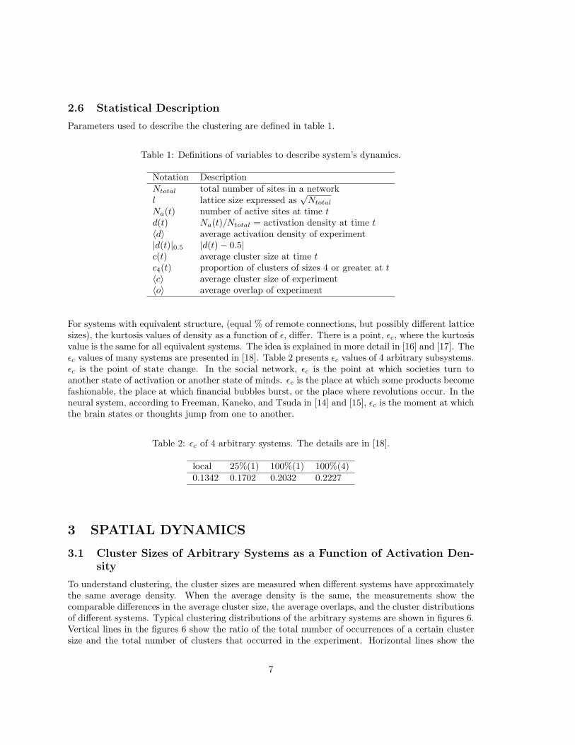
2.6 Statistical Description

Parameters used to describe the clustering are defined in table 1.

Table 1: Definitions of variables to describe system’s dynamics.

Notation DescriptionNtotal total number of sites in a networkl lattice size expressed as

√Ntotal

Na(t) number of active sites at time td(t) Na(t)/Ntotal = activation density at time t〈d〉 average activation density of experiment|d(t)|0.5 |d(t)− 0.5|c(t) average cluster size at time tc4(t) proportion of clusters of sizes 4 or greater at t〈c〉 average cluster size of experiment〈o〉 average overlap of experiment

For systems with equivalent structure, (equal % of remote connections, but possibly different latticesizes), the kurtosis values of density as a function of ε, differ. There is a point, εc, where the kurtosisvalue is the same for all equivalent systems. The idea is explained in more detail in [16] and [17]. Theεc values of many systems are presented in [18]. Table 2 presents εc values of 4 arbitrary subsystems.εc is the point of state change. In the social network, εc is the point at which societies turn toanother state of activation or another state of minds. εc is the place at which some products becomefashionable, the place at which financial bubbles burst, or the place where revolutions occur. In theneural system, according to Freeman, Kaneko, and Tsuda in [14] and [15], εc is the moment at whichthe brain states or thoughts jump from one to another.

Table 2: εc of 4 arbitrary systems. The details are in [18].

local 25%(1) 100%(1) 100%(4)0.1342 0.1702 0.2032 0.2227

3 SPATIAL DYNAMICS

3.1 Cluster Sizes of Arbitrary Systems as a Function of Activation Den-sity

To understand clustering, the cluster sizes are measured when different systems have approximatelythe same average density. When the average density is the same, the measurements show thecomparable differences in the average cluster size, the average overlaps, and the cluster distributionsof different systems. Typical clustering distributions of the arbitrary systems are shown in figures 6.Vertical lines in the figures 6 show the ratio of the total number of occurrences of a certain clustersize and the total number of clusters that occurred in the experiment. Horizontal lines show the

7

cluster size normalized with the largest possible cluster.

10−4 10−3 10−2 10−1 10010−9

10−8

10−7

10−6

10−5

10−4

10−3

10−2

10−1

100

normalized cluster size

prop

ortio

n of

occ

uren

ces

10−3

10−7

10−6

10−5

local 25% (1) 100% (1)100% (4)

local ε=5% ⟨c⟩=1.12 ⟨o⟩=6.7% std(o)=0.96% ⟨d⟩=5.13% std(d)=0.17%

25% (1) ε=5% ⟨c⟩=1.25 ⟨o⟩=6.5% std(o)=0.92% ⟨d⟩=5.13% std(d)=0.17%

100% (1) ε=5% ⟨c⟩=1.255 ⟨o⟩=6.35% std(o)=0.87% ⟨d⟩=5.11% std(d)=0.17%

100% (4) ε=5% ⟨c⟩=1.26 ⟨o⟩=6.32% std(o)=0.86% ⟨d⟩=5.11% std(d)=0.17%

10−4 10−3 10−2 10−1 100

10−8

10−6

10−4

10−2

100

normalized cluster size

prop

ortio

n of

occ

uren

ces

local 25% (1) 100% (4)

local ε=13.2% ⟨c⟩=3.2 ⟨o⟩=52.21% std(o)=7.2% ⟨d⟩≈26.58% std(d)=5.17%

25% (1) ε=15.5% ⟨c⟩=69.8 ⟨o⟩=46.20% std(o)=1.75% ⟨d⟩≈26.17% std(d)=0.88%

100% (4) ε=18.5% ⟨c⟩=281.6 ⟨o⟩=38.00% std(o)=0.99% ⟨d⟩≈26.1% std(d)=0.47%

Figure 6: Average clusters and overlaps for different systems in a lattice size 128 × 128. Left:〈d〉 ≈ 0.05. Right: 〈d〉 ≈ 0.26. As there are more remote connections the links among sites get moredistributed. There is less redundancy of connection overlapping. Consequently, 〈c〉 of the networkswith more remote connections is larger, but 〈o〉 is smaller.

The average cluster size in less structured networks is bigger for the same activation level, whencompared to more structured networks, (figure 6). Adding remote connections to the local systemsbreaks apart the clusters, which spread through the local connection. Remote connections can breakthe clusters, but can also create possible new ones, (e.g. in figure 1). Importantly, the average clustersize is bigger in the systems with relatively more one-way remote connections.

3.2 Supportive and Unsupportive Clusters

Cluster parts can be supportive or unsupportive. In the supportive cluster parts, all the sites in thecluster have the same activation value as the majority of their neighbors. If a site in the cluster hasan activation value different form its neighbors’ majority, the site is in the unsupportive part of thecluster. An example of a cluster whose sites support each other to stay together in the cluster, anda cluster whose sites do not support each other as strongly is in figure 7.Clusters are more supportive in more structured networks. Consequently, the biggest clusters occurin the networks without remote neighbors, having the same density level, (figure 6). Clusters thatspread locally are more static and they do not break easily, so they have a better chance to grow.

3.3 Why Do Remote Connections Make an Average Cluster Bigger?

The connections are more distributed among the sites in the system when sites have more one-way influences. Figure 3 explains structural differences of neighborhoods, but also shows that withthe addition of remote connections, more sites influence each other directly, even though the totalnumber of connections in the system does not change. Every site has the neighborhood of five. Withmore remote connections, there is less of a connection overlapping, so there is the same number ofconnections in total, but they directly connect more sites. In the extreme case, c in figure 3, whenthere are four remote connections per site, the site is one connection away from eight other sites. Inthe other extreme case, when the system is described by local model, case a in figure 3, the site is oneconnection away from four sites. Simulation results, measuring 〈c〉 as a function of number of remote

8

unsupportive�

y y y yyyy

y y yyy i ii i�����

supportive

y y y yyyy

y y yyy i ii i

Figure 7: An example of an unsupportive (left) and a supportive cluster (right). The majority rulehelps the cluster on the right retain its current activation. Remote connections break the majoritysupport for the cluster on the left. In the unsupportive part of the figure, a cluster most likely breaksapart in a series of steps if ε is small. For small ε, a supportive cluster most likely stays together.

connections of four typical systems, are in table 3. To make the arbitrary systems comparable, 〈c〉as a function of ε is measured keeping 〈|d|0.5〉 and 〈d〉 at the same level.

Table 3: 〈c〉 of four arbitrary systems in lattice size 128× 128.

〈d〉 ≈ 5% 〈d〉 ≈ 26% 〈|d|0.5〉 ≈ 11%local 1.12 3.20 6.0225%(1) 1.25 69.8 2868.4100% (1) 1.255 72.4 3779.8100%(4) 1.26 281.6 4324.1

4 MEASUREMENTS OF CLUSTERS AND OVERLAPS

4.1 Average Cluster Size

Both the average activation density and the average cluster size vary continuously as the function ofε up to a unique point, εc, at which the average density and the average cluster size exhibit powerlaw behavior. Figure 8 shows an example of normalized 〈c〉 and 〈d〉 in lattice size 128 × 128. If allthe variables describing the system are the same, but its size, the kurtosis of the system’s activationis greater below εc and lower above εc in the smaller systems. As the ε below εc increases, thedifference between the kurtosis of the smaller system and the kurtosis of the larger system becomessmaller. At εc the kurtosis is same for any system size. For ε greater then εc, the kurtosis of thesmaller system is smaller than the kurtosis of the larger system.Measure of kurtosis for calculating εc was used by Binder in [16], also. Binder defines

U(l, ε) =〈(d− 0.5)4〉〈(d− 0.5)2〉2

(3)

where d in the equation 3 can be substituted with c to measure the kurtosis with the average clustersize per a step. To describe power law behavior with critical exponents ν, β, and γ see [19]. A good

9

0 0.05 0.1 0.15 0.20

0.05

0.1

0.15

0.2

0.25

0.3

0.35

0.4

0.45

0.5local 25%(1) 100%(1)100%(4)

0.5−|d|0.5

ε 0 0.05 0.1 0.15 0.2

0

0.1

0.2

0.3

0.4

0.5local25%(1)100%(1)100%(4)

⟨c⟩ / 2⟨c⟩max

ε

Figure 8: 〈0.5− |d|0.5〉 and normalized 〈c〉 as a function of ε for system without remote connections.〈c〉 is normalized, so it is comparable with 〈0.5− |d|0.5〉.

example by Makowiec is in [17]. Using equations 4, 5, 6, and 7 to obtain linear interpolations of thevalues εc and critical exponents are found for the typical systems, (figure 9).

∂U(l, εc)∂ε

∼ l1ν (4)

〈|d(l, εc)|2〉 ∼ l−2β/ν (5)

〈χ(l, εc)〉 ∼ lγ/ν (6)

〈χ(l, εc)〉 = l2(〈d2(l, εc)〉 − 〈d(l, εc)〉2) (7)

0.1675 0.168 0.1685 0.169 0.1695 0.17 0.1705 0.171 0.1715 0.172 0.17251

1.2

1.4

1.6

1.8

2

2.2

2.4

2.6

2.8

3

0.1695 0.17 0.17052

2.05

2.1

2.15

2.2

l64 l80 l96 l112

ε

⟨(d−0.5)4⟩ / ⟨(d−0.5)2⟩2

0.2215 0.222 0.2225 0.223 0.2235 0.224 0.2245 0.225 0.2255 0.226 0.22651

1.2

1.4

1.6

1.8

2

2.2

2.4

2.6

2.8

3

0.22250.22260.22270.22280.22292.12

2.14

2.16

2.18

2.2

64 l80 l96

ε

⟨(d−0.5)4⟩ / ⟨(d−0.5)2⟩2

Figure 9: Estimate of εc with Binder’s method for 25%(1) and 100%(4): 0.1702, and 0.2227,respectively. Estimate of critical exponents: ν25%(1) = 0.9504, ν100%(4) = 0.9026; β25%(1) =0.3071, β100%(4) = 0.4434; γ25%(1) = 1.1920, γ100%(4) = 0.9371.

10

4.2 Cluster Overlapping

The perfect overlap by random activation of a given number of sites is very unlikely, so 〈o〉 isuseful as a supportiveness or stability measure of clusters. Table 4 shows the relationship betweenaverage activation density and the four arbitrary systems in terms of 〈o〉. The overlap at each stepis normalized with the average density of that step, since an overlaps bigger than the total numberof active sites cannot occur.

Table 4: 〈o〉 of four arbitrary systems with lattice sizes 128× 128.

〈d〉 ≈ 5% 〈d〉 ≈ 26% 〈|d|0.5〉 ≈ 11%local 6.70% 52.21% 66.56%25%(1) 6.56% 46.26% 60.66%100%(1) 6.35% 40.04% 56.44%100%(4) 6.32% 38.00% 54.27%

Having the average density level same, the overlapping is lower in less structured systems. Moresupportive structure preserves once formed clusters more likely. Interestingly, figure 10 shows that〈o〉 precedes the sudden jump of 〈0.5− |d|0.5〉.

0.12 0.13 0.14 0.15 0.16 0.17 0.18 0.19 0.2 0.21 0.220.15

0.2

0.25

0.3

0.35

0.4

local 25%(1) 100%(1)100%(4)

⟨o⟩ / 2⟨o⟩max

ε

Figure 10: 〈o〉 vs. 〈0.5−|d|0.5〉 as the function of ε for four arbitrary systems. Dotted lines represent〈0.5 − |d|0.5〉 of local, 25%(1), 100%(1), and 100%(4) systems, (from left). Unconnected shapesrepresent same systems but in terms of normalized overlaps. 〈o〉 is normalized, so it is comparablewith 〈0.5− |d|0.5〉.

4.3 Clusters for a Jump

Starting with a lattice system with randomly initiated site activations and small value of ε, after ashort time, the activity of the network stabilizes in either mostly active or mostly inactive mode ofbehavior. Because the systems are of finite size, they jump after a while from one mode of behaviorto the other, see figure 11. Jumps from the mostly inactive system to mostly active, and vice versa,take a relatively short time and occur more frequently, as the ε increases.

11

0 1 2 3 4 5 6 7 8 9 10

x 105

0

0.1

0.2

0.3

0.4

0.5

0.6

0.7

0.8

0.9

1

time

dens

ity

Figure 11: Typical temporal behavior of the active sites for 106 steps. 5% of randomly selected sitesin a lattice have one remote neighbor. Lattice size is 128 × 128. Jumps from the mostly inactivesystem to mostly active, and vice versa, take a relatively short time. What does happen with theclusters, to cause the system activation jumps? The size of supportive cluster helps.

What does happen with the clusters to cause the system activation jumps? In short, supportiveclusters help their sites retain the same activation, see figure 7. As the clusters grow, due to thesupport the sites of the same activation give to each other, the jumps are more likely. The measure ofproportion of clusters larger than four, 〈c4〉, is used to show that the proportion of supportive clustersincreases before the jump, and before the system’s average activation starts to change significantly,see figure 13. There are few configurations with four sites and just one is supportive, but stillthere have to be at least four sites in the supportive cluster. For examples, see figure 12. Clusterconfiguration in higher dimensions is an unsolved problem, see [20]. At the present, the computersimulation techniques are more helpful than analytical approaches.

iiiiiiiiiiiiii

iiii

ii

2 8 4 4 1

Figure 12: All cluster configurations on the square lattice for c = 4. Mirror images and rotatedconfigurations are not shown. The total number of each configuration is below the cluster image.Cluster configuration in 2-dimensions is an unsolved problem.

For 〈c4〉 as a function of ε, it is assumed that the similar spatial phenomenon occurs in both cases,when the jump occurs due to the system’s finite size, or when the jump occurs due to the suddenstate transition. Since the cluster configurations are not currently solved analytically, computersimulations are used to obtain the solutions of problems with higher than 1-dimension lattices.

12

0.13 0.14 0.15 0.16 0.17 0.18 0.19 0.2 0.21 0.220.2

0.22

0.24

0.26

0.28

0.3

0.32

0.34

0.36

0.38

0.425%(1) 100%(1)100%(4)

⟨c4⟩ / 2⟨c

4⟩max

ε

Figure 13: The proportion of clusters of sizes four or greater in all cluster sizes as a function ofε precedes the sudden jump of 〈0.5 − |d|0.5〉 (connected points). l=128. 〈c4〉 is normalized, so itis comparable with 〈0.5 − |d|0.5〉. Bigger and more supportive clusters prepare the system for thechange of general behavior.

5 CONCLUDING REMARKS

Activation clustering behavior is described in terms of 〈c〉, 〈o〉, and 〈c4〉. 〈c〉, 〈o〉, and 〈c4〉 are studiedas the functions of number of remote connections and as the functions of ε. All functions show powerlaw behavior. In particular, 〈c〉 and 〈|d|0.5〉 as the functions of ε, exhibit sudden transitions at thesame ε value, while 〈o〉 and 〈c4〉, as the functions of ε, precede 〈c〉 and 〈|d|0.5〉 with the suddentransitions. With the addition of one way connections, the distribution of communication means iseffectively increased. There are fewer repetitive links and the messages get across in fewer steps. Onthe other hand, with fewer remote connections, cluster structures are more static and more proneto the global change. Clustering depends on the supportive structure of the sites’ connections. Themore structured is the system, the more static or supportive the clusters are. Supportiveness isquantitatively described with 〈o〉. When different systems are compared, 〈o〉 values are higher in themore structured ones. What does it mean for the social and neural networks? It means that societiesin which individuals mutually listen each other stronger change easier due to noisy influences. Thenetwork states in which individuals communicate in closed cycles are more fragile then the statesof social networks where individuals communicate in one-way directions. 〈c4〉 as a function of εexplains what occurs spatially with the clusters as ε is varied. It shows that the clusters get biggerand more supportive before the sudden transition is about to take place. This makes the systemready to jump to another mode of behavior. 〈c4〉 can indicate what kind of activation clustering isnecessary for a fashion fad to start, a social revolution to occur, a financial bubble to burst, or another form of state transition to emerge. With the fast cooperation of many neurons forming a brainstate, the activity of a brain jumps through a trajectory of its states. To make the jump possible,supportive structures must organize to cause transitions between the thoughts, which govern thegoal-directed behaviors. To understand the behaviors of neural and human societies, the mysteriesof supportive structures in networks have to be explored.

13

6 ACKNOWLEDGMENTS

This research is supported by NSF grant EIA-0130352.

References

[1] Gould, H.; Tobochnik, J.; Berrisford, J. Introduction to Computer Simulation Methods: Appli-cations to Physical System. Pearson Education, Upper Saddle River New Jersey, 1995

[2] Albert, R.; Barabasi, A. L. Statistical Mechanic of Complex Networks. Reviews of ModernPhysics 2002, 74, 47

[3] Bollobas, B.; Riordan, O. Mathematical Results on Scale-free Random Graphs. Handbook ofGraphs and Networks. Wiley-VCH Weinheim 2003, 1–34

[4] Bollobas, B.; Riordan, O. The Diameter of a Scale-free Random Graph. Combinatorica. 2004,24, 5–34

[5] Newman, M. E. J. Models of the Small World. J. Stat. Phys. 2000, 101, 819-841

[6] Strogatz S. H. Exploring Complex Networks. Nature. 2001, 410, 268-276

[7] Dorogovtsev, S. N.; Mendes, J. F. F. Scaling Behavior of Developing and Decaying Networks.Europhys. Lett. 2000, 52, 33-39

[8] Zalanyi, L.; Csardi, G.; Kiss, T.; Lengyel, M.; Warner, R.; Tobochnik, J.; Erdi, P. Properties ofa random attachment growing network. Physical Review E 68. 2003, 066104

[9] Jin, E. M.; Girvan, M.; Newman, M. E. J. The Structure of Growing Social Networks. WorkingPapers. 2001, 01-06-032, Santa Fe Institute

[10] Watts, D. J.; Strogatz, S. H. Collective Dynamics of ’Small World’ Networks. Nature. 1998,393, 440-442

[11] Watts, D. J. Small Worlds. Princeton University Press, Princeton 1999

[12] Simon, H. A. A Behavioral Model of Rational Choice. The Quarterly Journal of Economics,Vol. LXIX, February, 1955

[13] Kozma, R.; Balister, P.; Bollobas, B.; Freeman, W. J. Dynamical Percolation Models of PhaseTransitions in the Cortex. In: Proc. NOLTA 01 Nonlinear Theory and Applications Symposium,Miyagi, Japan. Vol. 1. 2001; pp. 55-59

[14] Freeman, W. J. How Brains Make Up Their Minds. Columbia University Press, New York 1999

[15] Kaneko, K.; Tsuda, I. Chaotic Itinerancy. Chaos. 2003, 13 926-936

[16] Binder, K. Z. Phys. B. 1981, 43

[17] Makowiec, D. Stationary states of Toom cellular automata in simulations. Physical Review E55. 1999, 3795

14

[18] Kozma, R.; Puljic, M.; Balister P.; Bollobas B.; Freeman W.J. Neuropercolation: A RandomCellular Automata Approach to Spatio-Temporal Neurodynamics. Lecture Notes in ComputerScience. 2004, vol. 3305, pp. 435-443

[19] Stauffer, D.; Aharony, A. Introduction to Percolation Theory. Selwood Printing Ltd. 1994, WestSussex, GB

[20] Sykes, M. F.; Gaunt, D. S.; Glen, M.; Ruskin, H. J. Perimeter polynomials for bond percolationprocesses. Journal of Physics A 14. 1981, 287-293

15