Working Paper Research

Acquisitions, productivity, and profitability :Evidence from the Japanese

cotton spinning industry

by Serguey Braguinsky, Atsushi Ohyama, Tetsuji Okazaki and Chad Syverson

October 2014 No 270

NBB WORKING PAPER - OCTOBER 2014

Editorial Director

Jan Smets, Member of the Board of Directors of the National Bank of Belgium

Editoral

On October 16-17, 2014 the National Bank of Belgium hosted a Conference on “Total factor productivity: measurement, determinants and effects”. Papers presented at this conference are made available to a broader audience in the NBB Working Paper Series (www.nbb.be). Statement of purpose:

The purpose of these working papers is to promote the circulation of research results (Research Series) and analytical studies (Documents Series) made within the National Bank of Belgium or presented by external economists in seminars, conferences and conventions organised by the Bank. The aim is therefore to provide a platform for discussion. The opinions expressed are strictly those of the authors and do not necessarily reflect the views of the National Bank of Belgium. Orders

For orders and information on subscriptions and reductions: National Bank of Belgium, Documentation - Publications service, boulevard de Berlaimont 14, 1000 Brussels. Tel +32 2 221 20 33 - Fax +32 2 21 30 42 The Working Papers are available on the website of the Bank: http://www.nbb.be. © National Bank of Belgium, Brussels All rights reserved. Reproduction for educational and non-commercial purposes is permitted provided that the source is acknowledged. ISSN: 1375-680X (print) ISSN: 1784-2476 (online)

Acquisitions, Productivity, and Profitability: Evidence from the Japanese Cotton Spinning Industry*

Serguey Braguinsky, Carnegie Mellon University

Atsushi Ohyama, Hokkaido University

Tetsuji Okazaki, University of Tokyo

Chad Syverson, University of Chicago Booth School of Business and NBER

Abstract We explore how changes in ownership and managerial control affect the productivity and

profitability of producers. Using detailed operational, financial, and ownership data from the

Japanese cotton spinning industry at the turn of the last century, we find a more nuanced picture

than the straightforward “higher productivity buys lower productivity” story commonly appealed

to in the literature. Acquired firms’ production facilities were not on average less physically

productive than the plants of the acquiring firms before acquisition, conditional on operating.

They were much less profitable, however, due to consistently higher inventory levels and lower

capacity utilization—differences that reflected problems in managing the uncertainties of

demand. When purchased by more profitable firms, these less profitable acquired plants saw

drops in inventories and gains in capacity utilization that raised both their productivity and

profitability levels, consistent with acquiring owner/managers spreading their better demand

management abilities across the acquired capital.

* This research was funded in part by the Berkman Foundation at Carnegie Mellon University, Japan Society for thePromotion of Science (No. 25780155), and Initiative on Global Markets at the University of Chicago Booth School of Business. We thank three anonymous referees, Nick Bloom, Xavier Giroud, Jesse Shapiro, Bob Topel, Tatsuo Ushijima, and conference participants at the ASSA Meetings, the Stanford Conference on Japanese Entrepreneurship, NBER Summer Institute, FOM conference, and the NBER Japan Project for comments. Email: Braguinsky: sbrag@andrew.cmu.edu; Ohyama: ohyama@econ.hokudai.ac.jp; Okazaki: okazaki@e.u-tokyo.ac.jp; Syverson: chad.syverson@chicagobooth.edu.

1

1. Introduction

The influence of changes in corporate control of assets on productivity has been a focus

of theoretical and empirical research for some time. In principle, mergers and acquisitions can

reallocate control of productive assets to entities that are able to apply them more efficiently.

Besides increasing the productivity of the individual production units that are merged or acquired,

a broader process of such reallocations can also lead to aggregate productivity growth. Such a

mechanism therefore has the potential to explain patterns of productivity at both the micro and

macro levels. Implicit in the story of this mechanism—though not often treated explicitly in the

empirical work on the subject—is the notion that productivity growth occurs when changes in

ownership and control put assets in more able managers’ hands.1

Despite the comfortable intuition of this logic, previous research has not been fully

conclusive about the effects of ownership and management turnover. One clear cleft in the

literature (spanning both theory and empirics as well as multiple fields) is whether ownership

changes are indeed a mechanism to raise the productivity of inputs (Lichtenberg and Siegel, 1987,

Maksimovic and Phillips, 2001, Jovanovic and Rousseau, 2002, Schoar, 2002, and Nguyen and

Ollinger, 2006, are more recent examples of work supporting this view) or instead driven by non-

efficiency considerations like managerial hubris, market power, or investor irrationality

(examples backing such viewpoints include Roll, 1986, and Shleifer and Vishny, 2003).

2

While there could well be multiple motives for and consequences of ownership changes,

part of the literature’s ambiguity no doubt also reflects the inherent limitations of the data

available to earlier studies. For example, most datasets do not allow researchers to cleanly

distinguish between physical (quantity) productivity and revenue productivity, which can lead to

mismeasurement and incorrect interpretations (e.g., Foster, Haltiwanger, and Syverson, 2008,

Katayama, Lu, and Tybout, 2009, Syverson, 2011; Atalay, 2014, discusses the importance of

separating quantities from expenditures when measuring inputs). In particular, mergers or

acquisitions that increase market power will tend to lead to higher output prices for the merged

firm. In the typical revenue-based productivity measures of the literature, this would be reflected

as a measured productivity gain even absent changes in technical efficiency. These and related

1 The idea that managers or management practices—even independent of any considerations of ownership—shape differences in productivity across plants, firms, and even countries, is itself a focus of a separate, budding literature. Examples include Bloom and Van Reenen (2007 and 2010) and Bloom et al. (2013). 2 The literature’s size precludes comprehensive citation. Surveys include Jensen and Ruback (1983) and Andrade, Mitchell, and Stafford (2001). See also the collected works in Kaplan (2000).

2

measurement issues mean we are still limited in our knowledge of how turnover in asset

ownership and management affects producers’ efficiency levels.

In this paper, we seek to make progress on this front. A primary advantage of our effort is

a data set that allows us to investigate the production and input allocation processes at an unusual

level of detail. We observe the operations, financial reports, management, and ownership of the

universe of plants in a growing industry over the course of several decades (the Japanese cotton

spinning industry at the open of the 20th century). These data, which we describe in the next

section, contain records in physical units of inputs employed and output produced at each plant

in the years it operated as well as plant-specific output prices and wages and firm-level financial

data. We also collected information on all major ownership and/or management turnover events.

These combined data let us measure directly how such events were reflected in plants’ physical

productivity levels, profitabilities, prices, and other operational and financial metrics.

Our first set of findings draws a more nuanced picture of the effects of ownership and

management turnover than the straightforward “higher productivity buys lower productivity”

story that has motivated much of the previous theoretical and empirical work on efficiency-

enhancing mergers. Using our best measure of productivity described below (with physical

output and input quantities, the latter measured as service flows) we find that acquired firms’

production facilities were not on average any less physically productive than the plants of the

acquiring firms before acquisition. Both parties were equally adept at transforming physical

inputs into physical outputs, at least conditional on operating. We also find, however, that

acquired firms were much less profitable than acquiring firms prior to being acquired. These

findings echo an important strand in previous research that emphasized the role played by

assortative matching and profit-enhancing (but not necessarily efficiency-enhancing) synergies

(e.g., McGuckin and Nguyen, 1995, Rajan, Volpin, and Zingales, 2000, Rhodes-Kropf and

Robinson, 2008, David, 2014).

Therefore ownership/management turnover in the industry is best characterized as

“higher profitability buys lower profitability.” We use the uniquely detailed nature of our data to

dig deeper into the sources of pre-acquisition profitability differentials and to open the “black

box” of post-acquisition profitability improvement by disentangling its various components. We

find that pre-acquisition profitability gap did not result from large output price differences

between the firms. Nor do we see much evidence of increased market power contributing to

3

higher post-acquisition profits. Instead, as we show, the profitability gap reflected systematically

lower unit capital costs among acquirers, coming from two sources: lower average unrealized

output levels (inventories and sales for which payment had not been received) and systematically

higher capacity utilization. When these better acquirers bought less profitable establishments, the

acquired plants saw drops in unrealized output, gains in capacity utilization, and increases in

both their productivity and profitability. The pre-acquisition equality in physical productivity

between the acquired and the acquiring arose because, as we document below, acquired plants

had more productive capital of younger vintages. This canceled out their other disadvantages.

We thus show that despite similar initial productivity levels, efficiency gains along

several dimensions contributed to profitability growth for acquired establishments. Essentially,

more profitable companies took over firms that had better capital but were using it suboptimally.

By taking control of this superior capital and improving the manner in which it was employed,

the new management raised the acquired plants’ productivity and profitability.

As to the specific source of the better owners’ and managers’ advantage, the explanation

most consistent with the data is that better firms have a superior ability to manage the vagaries of

demand in the industry. (We describe just what this means in our context in the next section.)

This explanation is consistent not just with the productivity and profitability levels and changes

we observe, but also with the differences in inventory levels and capacity utilization. We present

a simple model that offers one possible mechanism through which this demand management

difference might operate.

The ownership and management reallocation process helped drive considerable

productivity growth in the industry. Between 1897 and 1914, industry TFP growth averaged an

impressive 2.5 percent per year, while about 70 percent of industry capacity changed hands

during our sample. And while acquirers were fairly concentrated—the asset reallocation process

resulted in the emergence of several very large firms—what set the leading firms apart was not

their market power (we show there was little) but rather the ability to acquire and fully utilize the

most productive capital.

While we focus our analysis on a single industry case study to take advantage of the

available data and unique setting, we believe that we offer broader lessons that shed light on the

current literature. It is worth noting that economic environment in Japan during our sample was

largely that of more or less unfettered capitalism, with much less government intervention than

4

became common later, and with corporations predominantly relying on equity to raise capital

(see, e.g., Miwa and Ramseyer, 2000). In particular, most Japanese firms in our sample (and all

important acquiring firms) were joint stock companies with diffused ownership, so that the

structures of ownership control and the scope of managers to influence outcomes were very

much like the structures and scope that exist today. Thus, the mechanisms we discover here could

easily operate in other industries, countries, and time periods; they might just be difficult to

isolate in standard datasets.

Furthermore, our data span a time of critical economic development and industrialization

for Japan, which was undergoing transition to modernity after 250 years of an isolated,

traditionalist society in what can be aptly described as a “self-discovery” process of development

(see Hausmann and Rodrik, 2003). Information as detailed as our data is unusual even for

producers in today’s advanced countries, to say nothing of developing countries whose situation

might be more similar to that of Japan at the time of our analysis. Hence we believe that broader

lessons regarding the development of an advanced industrial economy can be drawn from this

study. By digging deep into the micro-evidence, we aim to complement past empirical work and

provide fresh insights for further development of economic theory about resource reallocation.

2. Entry and Acquisitions in the Japanese Cotton Spinning Industry: Background Facts

The development of the Japanese cotton spinning industry in the late 19th and early 20th

centuries has long fascinated economists because of its unique nature “as the only significant

Asian instance of successful assimilation of modern manufacturing techniques” before World

War II (Saxonhouse, 1971; 1974).3

Figure 1 reveals that the development went through several stages. During the first stage,

The historical circumstances surrounding this development

made the story even more intriguing. Japan unexpectedly opened up to foreign trade in the 1860s

after 250 years of autarky. Cotton yarn, in particular, experienced the combination of the largest

fall in relative price from autarky to the free trade regime and the highest net imports (Bernhofen

and Brown, 2004). But starting from the late 1880s, the domestic cotton spinning industry began

a remarkable ascendance. Net exports turned positive for the first time in late 1896, and soon

after Japan was exporting a sizeable fraction of its output while imports became negligible.

3 To save some space, we present here a “bare-bones” sketch of these facts. More details can be found in Saxonhouse (1974) and Braguinsky and Hounshell (2014), building upon and expanding Saxonhouse’s study. See also Ohyama, Braguinsky, and Murphy (2004) and Braguinsky and Rose (2009).

5

Japanese knowledge of the technology was rudimentary, and as a result spinning mills were

small and unproductive. In 1887 there were 21 one-mill firms in the industry, with the average

mill containing only 4,022 spindles and employing 137 workers on the factory floor. By way of

comparison, average mill sizes were much larger in the United States (15,691 spindles), India

(25,022), and Britain (38,619)—see Rose (2000, p. 192) and Murayama (1961, p. 340).

The second stage involved the explosive growth of the 1890s and was ushered in by two

major innovations: the switch to longer-stapled raw cotton imported from India and the U.S., and

the adoption of a newer type of cotton spinning machinery. These two innovations were actually

closely linked. When Japanese producers were confined to short-stapled cotton grown

domestically or imported from China, they had to use specially adapted machines with below

state-of-the-art rotation speeds and other characteristics. (Thread spun from short-stapled cotton

is prone to breakage, and breakage rates rise with the spinning machinery’s speed and power

levels.) The switch to Indian and U.S. cotton allowed Japanese mills to import state-of-the-art

machines for the first time, making it an episode of technological “refinement” extensively

studied in the general growth literature (see the discussion below in Section 5 and in Appendix

D). By 1896, the average plant already had a capacity of 12,767 spindles and employed 719

workers. Over this decade of growth the number of firms and average plant capacity both tripled

while average plant employment rose fivefold. Combined with productivity growth, this caused

industry output in physical units to increase 17 fold during the same period.

Early industry entrants that had set up their production facilities before the major

innovations of the 1890s faced a disadvantage of being stuck with older vintage machines.

However, an important advantage some of them had developed by the time the innovations

happened was a superior ability to “manage sales.” Since this will play an important role in

mergers and acquisitions analysis below, we dwell upon this in some detail here.

Japanese cotton spinners at the time generally faced a very competitive market (see, e.g.,

Saxonhouse, 1971 and 1977). The market power of even the largest cotton spinning firms was on

par or below that of trading houses, so no producer could exercise much influence over the price

at which its yarn was being sold (Takamura, 1971, I: 325).4

4 Cotton yarn was also traded on the Osaka exchange, with gross transaction volumes being several times larger than output. Exchange prices strongly influenced what trading houses were willing to pay even in seemingly isolated local markets (Takamura, 1971, I: 327). Cotton spinning firms did take collective action to support prices by enacting output restrictions in slow years. By their nature, however, these restrictions affected all firms uniformly.

This does not mean, however, that

6

the playing ground was level across firms. Especially during slow demand, established trading

houses often limited their purchases to reputable producers with whom they had long-term

relationships (Takamura, 1971, II: 60-62). Selling outside of the network of large trading houses

entailed risks of its own, as unscrupulous traders could renege on contracts or their promissory

notes could bounce, failing to deliver real cash. We show below that these problems were indeed

severe, and the most successful early entrants (who later became major acquirers in the mergers

and acquisition market) managed these sales-related issues better than other firms early on.

This superior ability to manage sales may not have been crucial during the rapid

expansion phase, but we show in Section 4 that it started playing a major role in firms’ fortunes

when the industry’s development entered its third stage at the start of the 20th century. After

driving out most imports, the Japanese cotton spinning industry felt the limits of the market size

for the first time. Once the Boxer Rebellion effectively shut down the Chinese market in 1900,

the industry’s first major “overproduction crisis” was in full swing. Most of the following decade

saw industry consolidation with little if any growth on the extensive margin but with a lot of

acquisitions of existing production facilities, the first of which occurring in 1898 (Figure A1 in

Appendix C). Acquisitions were preferred over purchases of new machinery in part because the

average delivery lag for imported machine orders was 21.7 months during our sample, with a lot

of variance from year to year (Saxonhouse, 1971, p. 51).

These factors led to the consummation of 73 distinct acquisition deals involving 95 plants

(some changed hands more than once) between 1898 and 1920. All in all, 49 of the 78 plants—

63 percent of plants and 68 percent of capacity—that were in operation in the industry in 1897,

the year before the first acquisition took place, were subsequently acquired at least once.

Several large firms emerged from this process, mostly through serial acquisitions. These

were Kanegafuchi Boseki, Mie Boseki, Osaka Boseki (the latter two completed an equal merger

in 1914 to form Toyo Boseki), Settsu Boseki, and Amagasaki Boseki (the latter two merged in

1918 to form Dainippon Boseki). These five firms, which shrank to four after the 1914 merger

and to three after the 1918 merger, went from owning 10 percent of the plants and 25 percent of

industry capacity and output to 40 percent of plants and half of capacity and output over the 25-

year period of our analysis (Figure A2 in Appendix C). This concentration of ownership could in

principle be due to multiple factors, but as our empirical analysis below will show, it appears to

be sourced mostly in their superior ability to manage sales and as a consequence improve the

7

productivity and profitability of the plants they acquired.

3. Data

Our main data source is plant-level data gathered annually by various Japanese prefecture

governments and available in historical statistical yearbooks.5 For this paper, we have collected

and processed all the available data between 1899 and 1920. Because the first acquisition of an

operating plant in the industry happened in 1898, we added similar data for 1896-1898 using

annualized monthly data published in the Geppo bulletin of the All-Japan Cotton Spinners’

Association. Our data thus cover 1896 to 1920. Saxonhouse (1971, p. 41) declares that “the

accuracy of these published numbers is unquestioned.”6

Our data contain inputs used and output produced by each plant in a given year in

physical units. In particular, the data contain the number of days the plant operated, the average

daily numbers of spindles in operation and employees on the mill floor (male and female

separately), average daily wages by gender, data on intermediate inputs such as the consumption

of raw cotton, output of the finished product (cotton yarn) in physical units and its average count,

and the average price per unit of yarn produced. We observe which firm owns each plant at a

given time, so we can compare plant-level outcomes before and after ownership changes.

We match these plant-level data with financial data from semi-annual reports issued by

the firms that owned the plants. Those reports, which we were the first to systematically digitize,

contain detailed balance sheets and profit-and-loss statements as well as lists of all shareholders

(with the number of shares they held) and executive board members. Select financial data from

company reports were also published in the semi-annual publication Reference on Cotton

Spinning (Menshi Boseki Jijo Sankosho) which started in 1903. We use these data to supplement

company reports where they were missing.

Several unique properties of our research variables need to be explained in some detail.

First, cotton yarn is a relatively homogeneous product, but it still comes in varying degree of

fineness, called “count.”7

5 We describe only the most important features of our data here. A more detailed description is in Appendix A.

To make different counts comparable for the purpose of productivity

6 We checked anyway. We found occasional, unsystematic coding errors as well as obvious typos that we could often correct by comparing them with annualized monthly data from Geppo. In the vast majority of cases, however, the annual data in statistical yearbooks and the annualized monthly data did correspond very closely (any discrepancies were only a few percentage points). We dropped about 5 percent of observations where the annual data contained in government statistical reports could not be corrected. 7 The yarn count expresses how many yards are contained in a pound of yarn, so it reflects the yarn thickness.

8

analysis, we converted various counts to the standard 20 count using a procedure detailed in

Appendix A. Second, we used plant-year-specific female-to-male wage ratios to convert units of

female labor to units of male labor.8 Third, in addition to the number of installed spindles and

total employment, we also have data on the actual number of days of the year the plant was

operating. In other words, the data offer us the unusual ability to directly measure the flow of

capital and labor services at the plant level rather than to infer them from capital and

employment stocks or through other proxies like energy use. This also allows us to measure

input utilization rates.

4. Empirical Analysis

On average, 4.3 percent of the industry’s mills were acquired per year during our sample,

with the aforementioned serial acquirers responsible for about 40 percent of all acquisitions.9

These acquisition episodes form the base of our estimation sample.

4.1. Differences between Acquirers and Targets before Acquisition

We first use our detailed data to see, before there were any acquisitions in the industry, if

there were systematic differences among firms that would eventually a) acquire other firms, b) be

acquired, and c) exit without either acquiring or being acquired. 10

We compute plants’ physical total factor productivity levels (henceforth TFPQ, for

quantity-based TFP) using capital and labor input flows, effectively measuring the plant’s

productivity conditional on it operating. Being able to measure input service flows separately

from stocks is a luxury typically unavailable in producer microdata (especially for capital inputs),

and as will become clear below, the distinction between this TFP measure and a more typical one

We compare these firms’

plants along several dimensions: physical (quantity-based) productivity, accounting profitability,

average output price, main count of yarn produced, the number of days of the year the plant is

operational, the average age of the plant’s spindles, and the firm’s age.

Higher-count yarn is thinner (finer) and sells at a higher price per pound than lower-count yarn. 8 Using female-to-male wage ratios to aggregate the labor input assumes that wages reflect the marginal productivity of each gender. All our estimates are robust to including the number of male and female workers separately in the production function estimations. 9 Table A2 in Appendix C presents year-by-year counts of acquired plants during our sample. This average acquisition rate is higher than the 3.9 percent acquisition rate for large U.S. manufacturing plants over 1974-1992 reported in Maksimovic and Phillips (2001) and the 2.7 percent rate in the LED plant sample from 1972-1981 used by Lichtenberg and Siegel (1987). 10 There were also a few surviving firms that did not participate in the acquisition market during our sample.

9

that uses input stocks instead is informative about the nature of our results. We compute TFPQ

by estimating a production function using the method proposed by De Loecker (2013), with the

residuals reflecting plants’ TFPQ levels.11 To measure profitability, we use firms’ reported net

earnings, divided by the amount of paid-in shareholders’ capital.12 Equipment age is calculated

as the current year minus the equipment vintage year, where vintage year reflects the

composition of the years the plant’s machines were purchased. Firm age, on the other hand, is

always equal to the calendar year minus the year the firm was founded (defined as the year the

firm came into existence, which mostly coincides with the year it was incorporated).13

Table 1 shows means and standard deviations of the aforementioned plant characteristics

for each group of firms. We separate plants of future target firms into those that started operating

before 1892 (labeled “first cohort”) and those that started operating in 1892 or later (“second

cohort”), as the former are more likely to have older-vintage capital. The table includes only data

from 1896-97, before any acquisitions took place in the industry, and it excludes observations on

a few second-cohort plants whose first, partial year of operation was in 1896 or 1897.

Looking across the table’s top row to compare the average physical productivity levels

across the groups of plants, we see that plants in future acquiring firms—conditional on the plant

operating—are not more physically efficient than those in future acquired firms. Indeed, the most

efficient group of plants is the second cohort of the acquired. On the other hand, the ubiquitous

result in the literature that exiting plants are less productive than continuing establishments is

borne out in our data.

This pattern is reversed when we look at profitability. The most profitable establishments

(significantly so) are those in firms that will be acquirers. Plants in the first cohort of target firms

are the second-most profitable, and exiting and second-cohort acquired plants follow up the rear.

The numbers in the table’s third through fifth variable rows indicate these profitability

gaps are not tied to differences in the prices the plants fetch for their output. As seen in the third

11 The adaptation of this method to our setting is described in detail in the following section. We also show in Appendix F that our results are robust to alternative production function estimation methods. 12 We do not have firm balance sheets data for 1896-97, but we do have these for subsequent years, so we will also measure profitability as return on total capital employed. See Sections 4.2 and 4.3. 13 As the plant’s capital stock includes also buildings and various elements of infrastructure, equipment (spindles) age adjusted for vintage this way makes the plants look younger than they actually are. Firm age, on the other hand, certainly makes those plants that had added new spindles (or scrapped old ones, which is also captured in our measurement) look older than they are. Equipment age thus provides the lower bound, and the firm age the upper bound, for the true overall plant age.

10

row, all firms earn more or less similar prices per unit weight of output. Furthermore, future

acquirers produce higher (finer) counts of yarn. When we adjust for this fact by regressing the

logged unit-weight prices on indicators for the plant’s main count produced (counts were

aggregated into deciles and year dummies were included), we see from the fourth row that

acquirers’ count-adjusted prices (the residual from this regression) are even somewhat lower than

those of other firms. None of the groups’ average price residuals are significantly different from

zero, however. Thus profitability is not about plants earning supernormal prices relative to other

similar producers. This result, which we will see in other guises below, supports what we know

about the industry’s output market institutions: pricing did not reflect large market power

differences across industry producers and is unlikely to contribute to firm- or plant-level

outcomes examined in this paper.

The days-in-operation and age comparisons at the bottom of the table offer insight into

the possible sources of the productivity and profitability patterns. We saw that second-cohort

acquired plants are more productive than other plants, yet less profitable. Their productivity

advantage is tied to the fact that they have significantly newer capital (whether measured by

equipment or firm age), as reflected in the table’s final rows.14 A hint at why their productivity

advantage did not yield a profitability advantage can be seen in the comparison of plants’ average

days in operation. Second-cohort acquired plants operated almost a full working month less than

plants in future acquiring firms did. They were efficient while operating, but they were operating

considerably less often. Plants that were to exit the industry had the worst of both worlds: their

capital was old (not only were they the oldest firms, their equipment and firm ages were almost

the same, indicating they did almost no upgrading of their equipment), and their factories were

often idle. They were unproductive and unprofitable as a result.

4.2 Empirical Specifications

The analysis in the previous subsection revealed some systematic pre-acquisition

differences between acquiring and target firms. In particular, we saw that although acquiring

firms were more profitable, their plants were not necessarily physically more productive,

conditional on operating. Now we begin investigating whether and how acquired plants’

14 In Appendix D, we use additional data on firms’ orders of specific pieces of capital equipment to measure how the machines’ technical specifications evolved over time. We find clear evidence of pre- and post-early 1890s differences (not sensitive to the choice of a specific cutoff year around this general timeframe) along multiple dimensions: spindle rotation speed, spindles per frame, ability to handle multiple yarn counts and cotton types, etc.

11

performance metrics change when they are taken over by acquiring firms.

To measure plants’ productivity, we first estimate a production function. As shown in

Appendix F (Table A6), even a naïve calculation of TFPQ using residuals from an OLS

production function regression shows a substantial post-acquisition TFPQ increase (Table A6 in

Appendix F). Capacity utilization also rises (Appendix G). The fact that input use appears to

systematically adjust when ownership changes means that standard approaches to measuring

productivity effects of acquisitions, which assume productivity evolves exogenously, could bias

the estimates by attributing too much of any output gains to input use rather than changes in

productivity. 15

Following De Loecker (2013), we assume that the production function for plant i at time t

is given by

Hence as already mentioned we employ the productivity estimation method

proposed in De Loecker (2013). This approach accommodates endogenous productivity

processes and corrects for any simultaneous shifts in input use and productivity around

acquisitions, analogous to plants entering into exporting status in De Loecker’s investigation of

“learning by exporting”. Comparisons of the estimates below and those obtained using

alternative methods in Appendix F suggest that such a phenomenon may indeed be operating in

our setting in the period soon after acquisition, although estimated long-term acquisition effects

are similar across all methods.

𝑦𝑖𝑡 = 𝛽𝑘𝑘𝑖𝑡 + 𝛽𝑙𝑙𝑖𝑡 + 𝛽𝑖𝑖𝑖𝑡 + 𝛽𝑎𝑎𝑖𝑡 + 𝜔𝑖𝑡 + 𝜀𝑖𝑡, (1)

where y is logged output, k and l are respectively logged capital and labor flows (i.e., spindle-

days and worker-days), i is the change in logged plant capacity—total number of installed

spindles––from the previous to the current year (a control for any adjustment costs reflected in

production), and a is the logged age of plant capital. The term 𝜔𝑖𝑡 captures productivity and

subsumes the constant, and 𝜀𝑖𝑡 is a standard i.i.d. error. Productivity evolution is governed by

𝜔𝑖𝑡+1 = 𝑔(𝜔𝑖𝑡,𝑎𝑐𝑞𝑖𝑡) + 𝜉𝑖𝑡+1, (2)

where 𝑎𝑐𝑞𝑖𝑡 is a vector relating to a plant’s acquisition experience, and 𝜉𝑖𝑡+1 is an exogenous

productivity shock. In the baseline specification we assume that

𝑔(𝜔𝑖𝑡,𝑎𝑐𝑞𝑖𝑡) = ∑ 𝛾𝑗𝜔𝑖𝑡𝑗3

𝑗=1 + 𝜃1𝑙𝑏_𝑎𝑐𝑞𝑖𝑡 + 𝜃2𝑒𝑎_𝑎𝑐𝑞𝑖𝑡 + 𝜃3𝑙𝑎_𝑎𝑐𝑞𝑖𝑡, (3)

where we employ three sets of time dummies defined around each acquisition event: a “late pre-

acquisition” dummy ( 𝑙𝑏_𝑎𝑐𝑞𝑖𝑡 ) that equals 1 in the two years immediately preceding the

15 We thank an anonymous referee for pointing this out.

12

acquisition and zero otherwise, an “early post-acquisition” dummy (𝑒𝑎_𝑎𝑐𝑞𝑖𝑡) equal to 1 for the

first three years after the acquisition and zero otherwise, and a “late post-acquisition” dummy

(𝑙𝑎_𝑎𝑐𝑞𝑖𝑡) that equals 1 for all subsequent post-acquisition years after the first three and zero

otherwise.16 The predicted output in the first stage of De Loecker’s method is obtained by a

polynomial approximation using all inputs in (1) along with the proxy variables including three

acquisition timing dummies as above and (logged) cotton consumed in the production process.

Capital and labor input coefficients are identified from the following moment conditions:17

𝐸 �𝜉𝑖𝑡|𝑘𝑖𝑡𝑙𝑖𝑡� = 0 . (4)

The coefficients on labor and capital services flow inputs obtained from this specification

are estimated to be 0.323 and 0.738, respectively.18

We use these productivity estimates along with other plant performance measures to

investigate how acquisitions are related to changes in plant operations and performance. Because

of not enough number of post-acquisition observations on plants that were acquired very late in

the sample, acquisitions that happened in 1918 or later are excluded from estimations below. We

first look at changes within acquired plants. The estimating equations have the general form:

Our plant TFPQ measure is the residual from

the production function estimated using this approach.

𝑦𝑖𝑡 = 𝛼 + 𝜃1𝑙𝑏_𝑎𝑐𝑞𝑖𝑡 + 𝜃2𝑒𝑎_𝑎𝑐𝑞𝑖𝑡 + 𝜃3𝑙𝑎𝑎𝑐𝑞𝑖𝑡 + 𝑚𝐴 + 𝜇𝑡 + 𝜀𝑖𝑡, (5)

where yit is a performance measure of plant i in year t. The key right-hand-side variables are the

indicators for the three time periods discussed above: late pre-acquisition, early post-acquisition,

and late post-acquisition (the excluded early pre-acquisition period is also the same). We exclude

the acquisition year itself from the regression because acquisitions often happen mid-year,

16 We also estimated the production function with the cubic in specification (3) replaced by a linear approximation as well as by a cubic interacted with acquisition dummies (as in De Loecker, 2013, equation (10)). The results were very similar in all cases; see Appendix F. 17 This corresponds to equation (26) in Ackerberg, Caves, and Fraser (2006) and the timing assumptions discussed therein. Since both capital and labor inputs are measured as service flows in our baseline specification, it is natural to assume that these inputs are chosen simultaneously at the start of production. The quantity of cotton consumed in production, on the other hand, is inseparable from actual output produced, so it reflects all subsequent unobserved productivity shocks like stoppages due to breaking yarn, adjustments made to spindles rotation speeds, and so on. 18 As a check on the plausibility of these production function estimates, we compared this estimated labor elasticity to labor’s share of value added as computed from firms’ financial accounts. Assuming input adjustment costs aren’t too large, cost minimization implies these two values should be of similar magnitude. They were. While there is some ambiguity as to which line items in our cost data should be excluded from value added, the most inclusive assumptions imply an average wage share in our plants of 0.232, while the most exclusive imply a share of 0.485. Our estimated labor coefficient falls roughly halfway between these bounds. In addition to this check, we estimated the production function using several other approaches and found similar input elasticities. See Appendix F.

13

making it hard to attribute outcomes solely to the acquirer or the acquired.19

In a second specification, we look at productivity changes from before to after acquisition

events in a slightly different way. Namely, we compare acquired plants to the incumbent plants

of acquiring firms. This in effect uses the incumbent plants as a control group. We lose some data

as a result of this (namely, the cases where the acquirer came from outside the industry and hence

had no incumbent plants), limiting the exercise to 49 acquired plants. The benefit is that this

within-acquisition approach lets us explicitly compare plants’ productivity and profitability

changes while controlling for any specific circumstances of an acquisition.

The coefficients on

these period indicators will reflect how acquired plants’ performance measures change around

acquisitions. Because we are interested in looking at changes within plants, we include

acquisition fixed effects mA in the specification. These are identical to plant fixed effects for

plants that were acquired only once, the majority of our sample, but they allow us to control for

possible differences across acquisition events for plants acquired multiple times. We also include

year fixed effects µt to capture any industry-wide performance shifts over the sample.

20

The estimating equations in this case have the following form:

𝑦�𝑖𝑡 = 𝛼0 + 𝛽1𝐴𝐴𝑖𝑡 + 𝛽2𝐴𝑞𝑢𝑖𝑟𝑒𝑑𝑖𝑡 + 𝛽3𝐴𝑞𝑢𝑖𝑟𝑒𝑑𝑖 × 𝐴𝐴𝑖𝑡 + 𝑚𝑖𝑡 + 𝜇𝑡 + 𝜀𝑖𝑡 , (6)

where 𝑦�𝑖𝑡 is the outcome variable of plant i at time t if it is an acquired plant, while the outcome

variables of incumbent plants are collapsed to 𝑦�𝑖𝑡 = 1#𝑚𝐴

∑ 𝜔𝑗𝑦𝑗𝑡𝑗∈𝑚𝐴 , where 𝑚𝐴 denotes the

particular acquisition case in which plant i was acquired and #𝑚𝐴 is the number of incumbent

plants in acquisition 𝑚𝐴. Thus, 𝑦�𝑖𝑡 for incumbent plants is the weighted average of outcomes of

the plants within the given acquisition. The variable AAit is a dummy equal to 1 if acquisition mA

happened prior to year t and zero otherwise, and Acquiredi equals 1 if plant i is purchased in

acquisition case mA and zero otherwise. The acquisition-year fixed effect is mit, and µt is the

calendar year fixed effect. In the main text, we assign weights ωj = 1 to all incumbent plants in a

given acquisition mA, which allows us to interpret coefficients 𝛽1, 𝛽2, and 𝛽3 similarly to that in

19 We included all observations when estimating the production function using De Loecker (2013) method because it employs lagged values of various variables, making a time gap undesirable. In those estimations, the acquisition year is treated as part of the late pre-acquisition period. All our estimation results are robust to including the acquisition year into the (early) post-acquisition period or to dropping acquisition-year observations altogether. 20 To avoid problems stemming from the fact that plants previously acquired by serial acquirers are already “incumbent” plants when another acquisition happens, we only label a previously acquired plant as an incumbent after being under the new ownership for five years. The results presented below are not sensitive to other reasonable cutoffs or to using only serial acquirers’ originally owned plants in the “incumbent” category.

14

standard difference-in-difference estimations. In particular, �̂�3 reflects the change in acquired

plants’ performance around their acquisitions relative to the performance changes experienced

by the existing plants of their acquirers. We limit the sample time period to 4 years before and 8

years after the acquisition event, but reasonable alternative cutoffs produce similar results.21

We note that acquisition is, of course, not an exogenous occurrence. As is typical in this

literature, we do not have a source of random or even quasi-random assignment to acquisition, so

interpreting any of the plant performance changes around acquisition as isolating causal effects

should be done with caution. However, our specifications control for the most obvious sources of

potential biases by controlling for acquired plant fixed effects, removing any effects of selection

into acquisition on persistent plant attributes, and any common movements with various control

groups (the acquiring firms’ existing plants, for example). We are relying for causal inference in

part on the assumption that the causal effect of acquisition creates a discrete change in attributes

surrounding the event, whereas any performance trends that might lead to selection into

acquisition would be either common to the control plants and thus partialled out in our control

group specifications, or gradual enough to be distinguished from the more discrete direct effect.

To that end, we show in Appendix K that there are no obvious pre-trends in acquired plants’

relative performance, while at the same time there is a noticeable change in the trajectory of

certain performance measures at the time of acquisition.

4.3 Changes in Productivity and Profitability

Table 2 shows the results from estimating the within-acquired-plant specification (5) for

three outcome variables: TFPQ, plant profitability, and the count-adjusted price residuals

described in Section 4.1. It does so for the entire sample of acquisitions (the first three numerical

columns of the table) as well as the subsample of acquisitions done by the “serial acquirers”

discussed previously (the last three columns).

The results for TFPQ in the first numerical column indicate that in the first three years

after acquisition, acquired plants’ quantity-based TFP levels (conditional on operating) rose

about 4.5 percent above their pre-acquisition levels, a marginally statistically significant

difference. Subsequent years saw much more productivity growth, with the average TFPQ of

21 We also estimated equation (6) employing kernel weights obtained from the Mahalanobis distance measure where acquired and incumbent plants are matched on plant size, age and location, and also using a standard difference-in-difference procedure ignoring acquisition-based matching altogether. The results of these estimations were very similar to those presented in Table 3 (see Tables A7 and A8 in Appendix F).

15

acquired plants in the late post-acquisition period (i.e., more than three years after acquisition)

being more than 13 percent (e0.126 = 1.134) higher than their pre-acquisition baseline and

significantly higher than in the early post-acquisition period. Thus acquired plants’ TFPQ levels

improve considerably following acquisition, though it takes time for this to manifest itself fully.

The next column looks at acquired plants’ profitability around acquisition episodes. We

cannot directly evaluate plant-level profitability levels analogously to the cross sectional

comparisons in Table 1, for the obvious reason that there are no separate post-acquisition firm

profit accounts. We work around this issue by constructing a measure of plant-level net operating

surplus equal to the difference between the net value of cotton yarn produced by the plant and

plant labor and capital costs (see Appendix E for details). We then divide this by the sum of

shareholders’ capital (equity and retained earnings) and interest-bearing debt, which in case of

multiple plant firms is assigned to each plant in proportion to the plant’s installed spindle

capacity. We call the resulting measure “plant-level return on capital employed”—“plant ROCE”

for short—and we use this measure, Winsorized at the top two percent, to compare plant-level

profitability before and after acquisition periods.22

The results in the table indicate that the ROCE of acquired plants increases by an average

of about six percentage points in the first three years after acquisition. ROCE rises further in

subsequent years to a long-run gain of almost nine percentage points. Thus as a share of total

long-run gains, profitability growth occurs faster than the relatively back-loaded growth in

productivity. These are big changes in profit rates; the mean pre-acquisition ROCE of acquired

plants is about seven percent.

Finally, to see if changes in plant-specific prices contributed to profitability changes, we

estimate (5) using as the dependent variable the residuals from the regression of (logged) plant-

specific price on the deciles of yarn counts produced and year dummies. As already mentioned,

this reflects by how much the price of a given plant was above or below the average plant

making yarn of that count in a given year. The results, in Table 2’s third column, indicate that

post-acquisition prices are statistically indistinguishable from and economically similar to pre-

acquisition prices. Prices again do not explain profitability differences.

22 As shown in Appendix E, our constructed plant ROCE is highly correlated with firm-level ROCE data in years preceding acquisition events, when we have independent accounting data on both acquired and acquiring firms. The raw correlation between the two measures is about 0.7, and with the exception of extreme tails, the overall distribution fit is quite good too (Figure A6 in Appendix E).

16

We also test whether these productivity and profitability changes within acquired plants

are systematically related to the attributes of the acquiring firm. While acquiring firms could be

demarcated a number of ways, a natural one is whether they were one of the “serial acquirers”

we discussed in Section 2. We therefore run specification (5) while limiting the sample to

acquisitions by one of the five serial acquirer firms. The results are in the three rightmost

columns of Table 2. The patterns are qualitatively similar while being slightly more pronounced

in magnitude. Acquisitions by serial acquirers correspond to long run improvements in acquired

plants’ physical TFPQ of about 17 percent (e0.159 = 1.172) and ROCE increases of 14 percentage

points. The point estimates for price changes are larger than in the entire sample, but t-tests fail

to reject at conventional confidence levels equality of the coefficient on the pre-acquisition

indicator with either of the post-acquisition coefficients.

Overall, the within-plant results in Table 2 indicate that acquired plants see growth in

both their TFPQ and profitability levels after acquisition, though a greater share of long-run

growth occurs early on for profitability. These productivity and profitability changes are larger

for plants that are acquired by the most prolific of acquiring firms.

Table 3 presents similar comparisons using the within-acquisition difference-in-difference

framework of equation (6). Now the key variable of interest is 𝛽3 , the coefficient on the

interaction of the indicators for an acquired plant and for the post-acquisition period. This

coefficient shows how productivity, profitability, and prices change for acquired plants relative

to their average levels among the incumbent plants of the firm that acquires them. We again

estimate the specification for all acquisitions as well as the subsample done by serial acquirers.

In both TFPQ specifications, the estimates of the interaction coefficient 𝛽3 are positive

and statistically significant at the 1 percent level. The post-acquisition improvement of TFPQ of

acquired plants (this time relative to incumbent plants of the acquirer) averages about nine

percent for all acquisitions and about 12 percent for acquisitions by serial acquirers. In addition,

the acquired plant dummy coefficients are small in both samples, suggesting once again that

there is little systematic difference between the physical TFP of acquired and incumbent plants

prior to acquisitions (this is also observed in year-by-year estimations presented in Appendix K).

In the profitability regressions, �̂�3 is also positive and statistically significant. Profit rates

of acquired plants rise by four percentage points relative to acquiring firms’ plants in the whole

sample and by about six percentage points in acquisitions by serial acquirers. Here, the acquired

17

plant main effect is both statistically and economically negative, reflecting acquired firms’

profitability deficits before acquisition.

Once again, there are no differences to speak of in prices charged by acquired and

incumbent plants, both before and after acquisition events, although point estimates suggest a

small post-acquisition increase.

These results further reinforce what we saw in Table 2: acquisition was accompanied by

growth in the acquired plants’ productivity and profitability levels. We see here that this is true

relative not only to the acquired plants’ own levels before the acquisition, but also relative to

changes within incumbent plants owned by their acquiring firms.

4.4 Decomposing Profitability Differentials

When considered together, the findings above present a sort of puzzle. If it is neither

prices nor productivity, what makes incumbent plants more profitable than acquired plants before

acquisition? How do acquisitions by more profitable firms improve TFPQ in acquired plants?

Accounting Decompositions. We begin digging into this puzzle by decomposing plants’

profitability differences using our detailed financial data. Specifically, we decompose the pre-

acquisition profitability differential between acquiring and acquired firms as well as the pre- to

post-acquisition profitability changes for acquired plants into their various components. This lets

us isolate the most important factors driving profitability differences.

We first express a plant’s ROCE as the net value of cotton yarn produced and the plant’s

labor and capital costs (all per unit of capital assets):

( )1 ii i i i

i i i i

Y w L RC C C C

υπ −= − − . (7)

Here, is plant i’s operating income. Yi denotes the value of its output, and is the fraction of

intermediate input and non-labor operational costs in the value of output (e.g., the costs of raw

cotton, energy, etc.). Plant wage costs are wiLi, Ri is capital cost, and Ci is plant i’s share of its

owning firm’s capital employed (the sum of shareholders’ capital and interest-bearing debt). The

details of variable construction are described in Appendix E. In a nutshell, we use plant price and

output data to obtain Y and plant-level data on worker-days and average daily wages to obtain wL.

Capital cost is the sum of depreciation of fixed capital and interest payments on borrowed capital,

with both depreciation and interest rates assumed to be the same for all plants, as is the parameter

18

(these values are estimated from the available firm-level and industry-wide data). All nominal

values including capital employed are divided by the consumer price index to account for

inflation. Note that we did not have to do this in our regression analysis because our

specifications include year fixed effects.

We present the results of decomposition (7) in Table 4. The three panels each correspond

to the decomposition of a particular profitability differential. The top panel compares plants of

acquired firms (“acquired plants”) and those of their future acquirers (“incumbent plants”) for up

to 4 years prior to acquisition events. The bottom two panels compare acquired plants before and

after acquisitions, with the post-acquisition years split as in the regressions above: the middle

panel looks at the first 3 years immediately following the acquisition, and the bottom panel looks

at the subsequent post-acquisition years up to the 10th year.

The top panel of Table 4 shows that incumbent plants’ 5.1 percentage point ROCE

advantage over acquired plants is mostly explained by a net output value to total assets ratio (the

first term on the right hand side of (7)) that is on average 6.5 percentage points higher.23

The bottom two panels of Table 4 show the decomposition of acquired plants’ ROCE

changes around acquisition episodes. ROCE improves by 6.3 percentage points, and grows 10

percentage points in the longer run. As with the cross-sectional differences, most of the changes

came from growth in acquired plants’ ratios of net output value to total assets.

Wage

costs per unit of assets are actually higher in incumbent than in acquired plants, reducing the

ROCE difference. Capital costs are similar in size though statistically smaller for incumbents.

The centrality of net output value—essentially, gross margin—in explaining profitability

differences leads naturally to a second decomposition. We break the net-output-to-capital ratio

into a product of a) price, net of intermediate input and non-labor operation costs per unit output;

b) total input of capital and labor services per total assets; and c) TFPQ. Taking logs, we obtain

( ) ( )ˆexplog log log ii

i ii i

YY p TPFQC Cψ ψ

= + +

, (8)

where ψ ≡ 1 – υ is the unit price margin (common to all producers), pi is the plant’s output price,

23 The ROCE differential in the top panel of Table 4 is somewhat larger in magnitude than the acquired plant dummy coefficient in Table 3, where it was -0.03. The ROCE differentials in the middle and bottom panels of Table 4, however, correspond very closely to regression coefficients in Table 2, where they were 0.06 and 0.09, respectively. Reassuringly, the same holds when we compare most other computed differentials with the corresponding regression coefficients. Some discrepancy is to be expected, of course, as the regressions include acquisition fixed effects.

19

𝑌�𝑖 is the predicted output from the production function, and TFPQi is the production function

residual.24

As in the regression analyses, price and TFPQ differentials contribute relatively little to

the stark profitability differences between acquired and incumbent plants before the acquisition

(top panel). Most of the difference is instead driven by the ratio of predicted output (or combined

total inputs) to total assets, exp�𝑌�𝑖� 𝐶𝑖⁄ . The numbers in the top panel imply that for the same

amount of capital employed, incumbent plants manage to mobilize almost 30 percent more of

their combined inputs toward production than do acquired plants in pre-acquisition years.

This expression lets us measure the contribution of these three components to the net

value of output per unit of shareholders’ capital. These decompositions are presented in Table 5.

The decompositions of changes in acquired plants’ gross margins in the table’s bottom

two panels indicate input use intensity dominates early post-acquisition profitability growth, with

TFPQ growth mattering relatively more in the long run. This is similar to what we observed in

Table 2. In contrast to the regressions, price margins have a relatively large and statistically

significant long-run contribution, and TFPQ’s contribution is substantially larger than implied by

Table 2.25 The impact of the inputs-to-assets ratio, on the other hand, falls compared to the early

post-acquisition period, although it still contributes about a third of total increase in net output

value per unit assets.26

TFP Measure Decompositions. As a complement to the accounting decompositions, we

compare the TFPQ patterns we document above to what one would find if one had more

24 As we calculate TFPQ using output adjusted to a standard 20-count yarn as explained in Appendix A, we similarly adjust plants’ prices (which again are expressed per unit weight in the data). Specifically, we use the inverses of the conversion coefficients we use to adjust output. Adjusted output is obtained as 𝑦� = 𝑘𝑦, where y is output measured in weight and k is the conversion coefficient applied, and the adjusted price for the same count is �̂� = (1 𝑘⁄ )𝑝. This procedure ensures adjusted plant revenues remain the same as in the original data. 25 The reason for this difference is that the year fixed effects in regressions estimations effectively remove a time trend in productivity, while the TFPQ measure presented in Table 5 is best interpreted as inclusive of industry-wide productivity growth over time (which is itself partly a consequence of the acquisition process). Thus the regression coefficients give us a lower bound for TFPQ’s contribution to profitability growth (as they are stripped of any effect acquisitions may have on industry-wide productivity improvement over time), while the differentials in Table 5 represent the upper bound (“loading” all industry-wide productivity improvement into acquisition effects). We recomputed Table 5 using residuals from the production function estimations demeaned by industry-year averages and confirmed that TFPQ differentials in that case are closely aligned in magnitude with the regression coefficients. 26We show in Appendix G that this is not driven by a decline in capacity utilization rates. These in fact increasefurther in the long run, though at a more modest rate (we see this in another setting immediately below). The fall in the input-per-asset ratio observed in the bottom panel of Table 5 is instead an accounting phenomenon explained by a drop in the ratio of plant capacity to total firm assets. This drop is in turn driven by a big increase in acquired plants’ retained earnings (and therefore their shareholder capital). More detailed analysis of balance sheets (see Appendix G) indicates that retained earnings growth is related to firms’ increasing use of accumulated profits to finance new construction toward the end of the sample, where many of our late post-acquisition observations fall.

20

conventional producer microdata. Recall that our TFPQ metric has two distinguishing

characteristics: it measures output in physical units and it measures inputs as service flows rather

than stocks. Typical producer microdata contains only revenues as an output measure and capital

and labor stocks for inputs. As such, standard TFP measures tend to confound price and output

differences and embody variations in input utilization rather than conditioning on the plant

actually operating. Because the accounting decompositions above suggest a prominent role for

input utilization in explaining profitability differences across mills, this latter distinction between

our TFPQ and standard TFP metrics may be salient in our results.

We compute two alternative measures of TFP to explore this issue. One measures TFPQ

without conditioning on the plant actually operating. Specifically, when computing the residual

of the production function (3) to obtain TFPQ, instead of the input flows (spindle-days and

worker-days) used in our benchmark TFPQ metric, we use capital and labor stocks (spindles and

workers). This measure, which we call TFPQU (“U” for “unconditional” on operating), is shifted

by disparities in input utilization. Higher (lower) input utilization shows up as higher (lower)

TFPQU for a plant.

Our second alternative TFP measure further modifies TFPQU by adding to it the plant’s

logged output price. This mimics the revenue-based output measure typically used in the

literature. By construction, any difference between patterns in this productivity measure (which

we refer to as TFPR, using the standard nomenclature for revenue-based productivity) and

TFPQU comes from price differences across producers.

Using TFPR in specifications (5) and (6) reveals how our productivity results would look

if we had only standard producer-level microdata. Any contrast between such results and those

obtained above using our benchmark TFPQ metric reveals the combined influence of plant-level

heterogeneity in prices and input utilization. We can further use TFPQU to decompose this

contrast into the separate influences of price and input utilization differences.

The estimates of (5) and (6) with our three TFP measures are in Table 6. The left half of

the table shows the within-plant specification (5), the right half the within-acquisition difference-

in-difference specification (6). The results for our benchmark productivity measure TFPQ are the

same as those in Tables 2 and 3. We report them again here for convenience.

The TFPR results indicate a roughly 18 percent rise in this productivity measure relative

to the pre-acquisition baseline and an almost 34 percent increase in the longer term. These

21

changes are 2-3 times the size of the TFPQ gains estimated above. The difference-in-difference

results for TFPR tell a similar story. The interaction terms indicate acquired plants’ TFPR levels

rose post-acquisition about 16 percent more than among their acquiring firms’ incumbent plants.

The same gap in TFPQ terms was only about nine percent. Also unlike the TFPQ regressions,

both main effects are significant. Before acquisition, purchased plants had on average about eight

percent lower TFPR than their acquirers’ plants.

The specifications using TFPQU offer insights as to the source of the differences in the

TFPR and TFPQ results. In both the within-plant and difference-in-difference specifications, the

estimated TFPQU changes are quantitatively closer to their TFPR analogs than their TFPQ

counterparts. In fact, we cannot reject the hypothesis that the TFPR and TFPQU coefficients are

equal. Because TFPQU is shifted by variation in input utilization but is not affected by price

differences, the close tracking of TFPR by TFPQU implies that input utilization heterogeneity

explains most of the difference between our benchmark TFPQ results and those obtained using

the TFPR metrics typical of the literature. Price heterogeneity across plants, on the other hand,

explains little. Both of these results are consistent with both the regression and accounting

decomposition exercises above, which found few price differentials but substantial variation in

capacity utilization.

Putting these results together offers an explanation for the patterns documented in

Sections 4.1 and 4.2. Profitability and productivity conditional on operating both rise at acquired

plants after acquisition. In the short run, almost all profitability increases are the result of

increased input utilization rates rather than greater productivity conditional on operating. In the

longer run, conditional productivity TFPQ plays a larger role in raising profitability, though the

contribution of increased utilization is of similar size. This connection can be seen even more

clearly in Figure A14 in Appendix K where we present estimated effects of acquisitions on TFPQ

and TFPQU using a full set of annual pre- and post-acquisition year dummies.

4.5 The Link from Profitability to Productivity: The Role of Demand Management

Why were stronger firms able to utilize their inputs so much more than weaker firms? In

this section we tie these utilization differences to companies’ abilities to manage the industry’s

inherent demand variations.

As we discussed in Section 2, a lack of price differentiation does not mean that output-

22

market conditions were equivalent across firms. To quantitatively explore possible differences in

firms’ demand-facing operations, we investigate patterns in plants’ finished goods inventory and

accrued revenues on delivered output (that is, the payment for which is in arrears). We choose

these metrics because they may indicate when a plant is having difficulty finding buyers in a

timely manner or finding buyers who can be relied upon to disburse payments on time. These

conditions in turn may explain capital utilization differences.

Table 7 shows producers’ ratios of period-end finished goods inventories, accrued

revenues, and the sum of these (“unrealized output” for short) to their output over the period. We

split the sample by the same plant categories as in the previous decompositions.27

The top panel shows that incumbent plants’ ratios of unrealized output to their total

produced output value were about 60 percent lower than that of acquired plants before

acquisition. The bottom two panels indicate that after acquisition, acquired plants’ unrealized

output ratios fell 60 percent within the first three years and another 10 percent after that. Within-

acquisition comparisons of acquired and incumbent plants (not shown) yield similar patterns.

Thus whatever management abilities allowed acquirers to sustain lower unrealized output was

transferred to their acquired mills after purchase.

As to the specific sources of cotton spinning firms’ abilities to manage demand, there are

several potential explanations. While many of these are difficult to quantify, one important factor

already mentioned in Section 2 was that in low-demand times, major trading houses appeared to

limit their purchases by “sticking” with certain producers rather than cutting prices. At the time,

big trading houses were still much stronger financially than most spinning firms, and they often

had to extend credit to the latter (either directly or through forward purchases) during business

downturns (Takamura, 1971, I: 323-325; II: 60-62). High risks associated with this led the

traders to favor reputable and well run industry producers with whom they had established long-

term relationships. In turn, this allowed those producers to sustain more consistent operations,

resulting in the lower inventories and higher utilization levels observed above.

To explore this possibility quantitatively, we used the 1898 edition of Nihon Zenkoku

Shoukou Jinmeiroku, a nationwide registry of names of traders and manufacturers, to extract the

27 Finished goods inventories and accrued revenues are positively correlated in the data, but the correlation is modest, about 0.22 for both incumbent and acquired plants. There may be some direct connection between the two, as having difficulty finding reputable buyers in a timely fashion might lead a firm to reach out to lesser buyers who are more likely to fall into arrears. Therefore, total unrealized output seems to be the best metric to measure demand-facing operations efficiency. Nevertheless, all three metrics paint a consistent picture in Table 7.

23

names of individuals likely to play the most prominent role in cotton spinners’ output markets.

This yielded a list of 154 individuals.28

We then tested whether a producer’s relationship to trading houses is reflected in the

performance metrics we explored above. Table 8 compares the means for in-network and out-of-

network firms of TFPQ, TFPQU, ROCE, ratios of unrealized output to the value of output,

spindle utilization rates, and count-adjusted prices residuals. (Figures A8-A13 in Appendix H

plot the corresponding distributions.) Since our in- or out-of-network classification is based

primarily on the 1898 shareholders and board composition data, we limit our attention to years

1898-1902 to obtain a reasonable number of observations while not going too far forward, as

board and shareholders as well as traders’ importance of course changed over time.

We then matched these individuals to the lists of board

members and top 10-12 shareholders of the 67 firms for which we have company reports in 1898

(this is 90 percent of firms operating that year). Of a total of 1,197 board members and top

shareholders, 128 were on the list of the 154 most prominent traders described above. 33 of the

67 firms had at least one prominent trader among its board members and top shareholders. We

create an indicator equal to 1 if the firm is one of these 33 or one of two more firms for which

firm histories (Kinugawa, 1964) clearly indicated connectedness to major traders at their

inception (we refer to these as “in-network” firms) and 0 otherwise (“out-of-network” firms).

The results in Table 8 show that both average TFPQ levels and especially average

TFPQU levels—which register variations in capacity utilization as productivity differences—of

in-network firms’ plants are significantly higher than those of out-of-network firms. We observe

large ROCE differences across the two sets of plants as well. Furthermore, being in-network is

associated with a roughly 40 percent drop in plants’ unrealized output ratios. These mean effects

are reflected broadly across the distribution of plants: both the ROCE and unrealized output ratio

distributions of in-network firms are basically shifts of the corresponding out-of-network

distributions (see Figures A10-A11 in Appendix H). In-network firms also have higher capacity

utilization and prices, although these differences are relatively small and are not equally

pronounced across the distributions. The distributions of price residuals of in- and out-of-

network plants in particular are quite similar except for their far left and right tails, where some

28 These individuals fit into groups meeting one of three criteria. One group included 98 cotton yarn and yarn-related traders across Japan who paid more than 50,000 yen in operating tax that year. A second group included 25 individuals listed as board members of the 4 largest incorporated cotton yarn-related trade companies (Naigaimen, Nihon Menka, Nitto Menshi and Mitsui Bussan). Finally, the third group includes the 31 board members and traders registered at the Osaka cotton and cotton yarn exchange.

24

plants of in-network firms sell at very high prices (Figures A12 and A13 in Appendix H).

Overall, these results suggest that close relationships between industry producers and

prominent traders allowed connected producers to manage demand fluctuations more effectively,

particularly with regard to being able to operate with lower average inventories and greater

capacity utilization levels. Notably, in-network firms were also more likely to acquire other firms

in the future; the sample probability of being a future acquiring firm is 0.79 for in-network firms

as opposed to 0.21 for out-of-network firms. Hence, relationships with traders’ networks can help

explain why initial profitability gaps existed, and why they were closed by acquisition. The

accompanying TFPQ gains—improvements in efficiency even conditioning on operating—are

consistent with this mechanism if demand management is correlated with broader managerial

abilities that raised operational efficiency. We explore this connection in Section 5 below.

Another related factor that contributes to better plant and firm performance is having

chief engineers with formal technical education. In fact, having formally educated engineers in

charge has effects similar to and largely independent of being in-network, but even more strongly

pronounced in TFPQ (see Table A17 in Appendix L and the discussion therein).

4.6. Robustness

As already mentioned, we have conducted several robustness checks. We relegate the

details and presentation of the results to Appendix F for the sake of parsimony, but we briefly

describe the exercises here.

Our benchmark results above use TFPQ estimates obtained from a production function

estimated via one of the three specifications discussed by De Loecker (2013). While this presents

a way to deal with the classic transmission bias arising from a correlation between unobserved

productivity changes and producers’ input choices, we also estimated our specifications with

TFPQ constructed via alternative methods, including simple OLS, the Blundell and Bond (1998)

“system GMM” estimator, and two other specifications suggested by De Loecker (2013). In all

cases, the results were qualitatively and quantitatively similar to those above.

While matching by acquisition cases seems to be the most natural approach in our context,

we did explore other matching strategies. We matched acquired plants on pre-acquisition

characteristics and on pre-acquisition productivity trends with a control group of plants that were

either never acquired or, at least, not acquired within the time window during which we compare

25

them to acquired plants. The results of these estimations, presented in Tables A10 and A11 of

Appendix F, are very similar to the ones presented here.

Finally, we performed a simple placebo test by randomly assigning acquisition status to

plants and then estimating the relationships between our outcome variables and this randomly

generated acquisition status. We repeated this process 1,000 times and calculated the sample

mean of the estimated coefficients relating “acquisition” to outcomes. In most cases, the

magnitudes were only fractions of their analogs from the true acquisition sample.

5. A Mechanism

Our empirical results point to some sort of demand management ability, reflected

empirically in capital utilization levels and unrealized output rates, as being related to

productivity and profitability variation in both the cross section and over time within acquisition

events. Here we offer a simple theory that elucidates one channel through which fundamental

heterogeneity across owners/managers leads to variations in such ability, and through this, TFPQ

and profitability. If this heterogeneity is “carried” in acquisitions by owners/managers into target

plants’ operations, it explains the productivity and profitability changes surrounding acquisition

events estimated above. That said, it is possible that other possible mechanisms could explain the

data, and we cannot test the model’s time allocation implications directly because we do not

observe owners’/managers’ time allocations. Nevertheless, we find it useful to explicitly lay out a

set of conditions and economic decisions that can yield the empirical patterns above.

5.1 Plant Production and Demand

For simplicity, we focus on a case where each firm initially operates a single plant before

an acquisition opportunity arrives. A firm has access to the following production technology:

𝑦 = 𝑔(𝑚)𝑥𝜔 (9)

where 𝜔 is the given quality of a plant, and 𝑥 is the composite input of appropriately weighted

labor and capital. For example, if the technology is Cobb-Douglas, the composite would be the

plant’s inputs raised to their respective input elasticities. The function 𝑔(𝑚) is a flow of in-firm

services provided by the plant manager to increase outputs from a level of 𝑥𝜔. The variable m is

the manager’s time allocated to managing production. This is divided into time spent ensuring

that the plant operates at full capacity (therefore affecting input utilization), and time spent

improving efficiency of operations themselves. For example, the former may involve making

26

sure that machines are in working condition and that there are always enough workers to operate

them. 29 The time spent improving operational efficiency, on the other hand, would involve

monitoring the production process, receiving and acting upon reports from workers and

improving quality control.30 To ease notation, assume 𝑔(𝑚) = √𝑢𝑣, where u denotes the time

spent improving the frequency of operation (so that utilized input is given by 𝑥� = √𝑢𝑥), and v is

the time spent improving plant performance conditional on operating, thus augmenting the

intrinsic plant productivity, equal to 𝜔� = √𝑣𝜔.31

We assume that the firm first chooses x to minimize the cost of producing a given y and

then optimally chooses u, v, and y. Thus the input choice x is

We assume the total time spent managing the

plant 𝑚 = 𝑢 + 𝑣 is bounded between 0 and some 𝛾 > 0 , the manager’s effective time

endowment. We discuss this more below.

𝑥∗ = 𝑦√𝑢𝑣𝜔

, (10)

and the plant’s cost function is 𝑐(𝑦) = 𝑝𝑥𝑥∗ = 𝑦 √𝑢𝑣𝜔⁄ , where to simplify notation we have

normalized the price of 𝑥 to 1 by an appropriate choice of units.

The plant takes output price p (determined by the exchanges) as given, but its quantity

sold depends on managerial time allocation. Namely, it sells 𝛾 − 𝑚 units. Revenues are then

𝑟 = 𝑝(𝛾 − 𝑚). (11)

The quantity sold 𝛾 − 𝑚 is the channel through which we introduce the notion of demand

management; the plant’s demand depends on the time the manager allocates to selling product.

Because 𝑚 is the total time the manager devotes toward production, other things equal, a higher

𝑚 means less demand for output.

5.2 Optimal Allocation of Manager’s Time

From (10) and (11), the plant owner’s time allocation problem is

max𝑢,𝑣(𝛾 − 𝑢 − 𝑣) �𝑝 − 1√𝑢𝑣𝜔

�, (12)

where we have made use of m ≡ u + v. That is, the plant’s owner allocates his time between

29 Saxonhouse (1971) describes the problem of absenteeism in the industry. 30 Anecdotes about the importance of this sort of managerial activity are in, e.g., Kuwahara (2004) and Appendix B. 31 Diminishing returns are not necessary for the results below to hold. In particular, all of the analyses in this section go through if we instead assume input utilization and augmented plant quality are simply proportional to managerial time spent on these activities, so that 𝑥� = 𝑢𝑥 and 𝜔� = 𝜔𝑥, although derivations become more cumbersome.

27

managing plant production and managing demand (sales) so as to maximize profits. 32

It is easy to see (see Appendix I for the proof) that at the optimum, u = v = m/2. We can

thus restate (12) in terms of the optimal time allocated to production management, m:

The

optimal resource allocation problem (12) captures the fundamental tradeoff faced by the

manager: devoting more time to managing sales results in lower operational frequency and/or

efficiency, and vice versa. The constraint is set by the effective time endowment 𝛾; a higher 𝛾

reduces the lost revenue from any m. The parameter 𝛾 is thus interpreted as “demand

management ability”; this can include skill at building networking relationships with trading

houses, a reputation for reliable delivery, and perhaps the ability to effectively collect debt. It

might also be enhanced by having an educated engineer in charge of the plant, which presumably

allows the owner to spend more time managing sales and less on technical productivity issues.

max𝑚(𝛾 − 𝑚) �𝑝 − 2𝜔𝑚

�. (13)

The first order condition is sufficient and it yields (after some manipulation):

𝑚(𝛾,𝜔) = �2𝛾 𝑝𝜔⁄ and 𝜋(𝛾,𝜔) = ��𝛾𝑝𝜔 − √2�2𝜔� . (14)

A simple exercise yields the following results.

Lemma 1:

(i) 𝜕𝑥� 𝜕𝛾⁄ > 0 and 𝜕𝜔� 𝜕𝛾⁄ > 0. Input utilization 𝑥� and augmented productivity 𝜔� increase in 𝛾.

(ii) 𝜕𝜋(𝛾,𝜔) 𝜕𝛾⁄ > 0 and 𝜕𝜋(𝛾,𝜔) 𝜕𝜔⁄ > 0; also, 𝜕𝑥∗ 𝜕𝛾⁄ > 0. Profits increase in ability 𝛾 and

plant quality 𝜔, while total inputs also increase in 𝛾.

(iii) 𝜕2𝜋(𝛾,𝜔) 𝜕𝛾𝜕𝜔⁄ > 0. Ability 𝛾 and plant quality 𝜔 are complements in the profit function.

Proof: See Appendix I.

Lemma 1 implies increasing returns to demand management ability that are manifested

in both an increased span of control in production, 𝑥∗, and input utilization, 𝑥�. Augmented plant

efficiency 𝜔� also increases in demand management ability, implying that output increases with

ability even conditioning on inputs and their utilization. The first feature is consistent with our

decomposition results that showed more profitable firms (with higher demand management

32 We assume that p is greater than the plant’s marginal cost for at least some 𝑚0 < 𝛾, so that operation is profitable for all 𝑚0 < m < 𝛾. The (𝛾 − 𝑚) function limits the size of the plant, though it would be easy to introduce increasing marginal costs or downward sloping residual demand (say as in a monopolistically competitive structure) if one wanted to further constrain plant size.

28

ability) had higher input utilization rates. The second feature is consistent with TFPQ, measured

conditional on operating, increasing once a plant owned by a less profitable firm is acquired by a

more profitable firm. We explore this point more below. It is also in line with the findings in

Tables 8 that capacity utilization and TFPQ are higher for “in-network ”and 9 that capacity

utilization and TFPQ are higher for “in-network” firms and in Table A17 in Appendix L showing

the same for firms with educated engineers in charge.

5.3 Mergers and Acquisitions

We employ a model of asset reallocation through acquisitions similar to Jovanovic and

Braguinsky (2004) and Jovanovic and MacDonald (1994). Since our focus is on plant-level

profitability and productivity changes, we limit the exposition in the main text to the basics. See

Appendix I for the full setup and formalization of industry equilibria described intuitively below.

The industry evolves in three stages. In the first two, each firm can manage at most one

plant. In the first stage, an initial “basic” state of technological knowledge arrives, offering entry

by the industry’s first cohort of firms. The basic nature of this initial technological knowledge is

manifested in the low quality of plants, 𝜔1, available for this first entry cohort. Each entrant

comes into the industry with some initial demand management ability level, 𝛾0. First-cohort

producers have an opportunity to develop this ability above the initial level (for instance, they

make connections with traders or are able to hire an educated engineer). In equilibrium at the end

of the first stage, the first cohort’s ability is distributed with support [𝛾∗, 𝛾𝑚𝑎𝑥], where 𝛾∗ is a

threshold ability level and 𝛾∗ ≥ 𝛾0.

The second stage begins with an unanticipated change in the state of technology (a

“refinement,” in Jovanovic and MacDonald, 1994). As mentioned, such a refinement occurred in

Japanese cotton spinning when the industry developed new sources for raw cotton (imported

from India and the U.S.). This made it possible to import state-of-the-art machines from England

for the first time; see Appendix D. In the model, this is captured by a higher plant quality,

𝜔2 > 𝜔1, available to the second cohort of entrants.33

33 Jovanovic and MacDonald (1994) present a detailed account of one such refinement, the invention of the Banbury mixer, and how it affected the entry and exit of firms in the U.S. tire industry. Rajan, Volpin, and Zingales (2000) describe how another refinement, the advent of the radial, in the same industry more than half a century later led to its eclipse in the U.S. through acquisitions by foreign producers. More generally, a refinement can be interpreted as any investment-specific technological change embodied in new vintage capital or a new type of input (or both, as in our case). The issues related to such changes have been extensively studied in the macro growth literature (see, for

In the new industry equilibrium at the end

29

of this stage, the industry contains a mixture of incumbents with (differentiated) high ability

levels operating low-quality plants and new entrants with only basic ability but operating high-

quality plants (recall that each firm can only manage one plant at this stage). The threshold

ability of a marginal surviving firm in the second-stage equilibrium, 𝛾∗∗, is greater than the first-

stage threshold 𝛾∗. Hence some first-cohort firms exit at this stage.34

The third stage is characterized by an unanticipated opening of the market for

acquisitions. In this stage, each firm can potentially manage more than one plant and can

replicate its plant manager quality in a newly acquired plant.

35

In Appendix I we construct and formally solve for the asset reallocation equilibrium in

this stage. The key characteristics of this equilibrium are intuitive and can be summarized as

follows: (i) all second-cohort owners of high-quality plants sell their assets and their firms exit;

(ii) among first-cohort owners of low-quality plants, those with higher ability buy plants from

those with lower ability; (iii) because profits 𝜋(𝜔, 𝛾) are increasing in 𝛾 , the gains from

acquisitions are the highest when first-cohort entrants with especially high ability acquire high-

quality 𝜔2 plants formerly managed by the low-ability second cohort entrants.

There is no new entry during this

stage. Profitability and productivity growth is attained through the reallocation of production

facilities from firms with low demand management ability to those with high ability.

5.4 Implications for Productivity and Profitability

We now derive implications of the merger and acquisition process outlined above for

productivity and profitability of acquired plants. As we will show, the implications are consistent

with the patterns we document in Section 4.

To discuss the implications for productivity, note that a plant’s TFPQ in the model is

TFPQ ≡ 𝑦 𝑢(𝛾)𝑥⁄ = 𝑣(𝛾)𝜔. Lemma 1(i) implies that for a given 𝜔, TFPQ will increase with

the acquiring firm’s managerial ability 𝛾. Similarly, Lemma 1(ii) says that profits increase with

this ability. Because all acquisitions involve firms with higher ability acquiring a plant managed

by a firm with lower ability, these imply

example, Cooley, Greenwood, and Yorukoglu, 1997, and Jovanovic and Yatsenko, 2012), and may account for a major part of economic growth (Greenwood, Hercowitz, and Krusell, 1997). 34 See Jovanovic and MacDonald (1994). In our data, 10 out of 21 firms that had operated in the industry prior to the refinement of the early 1890s remained small and eventually exited by shutting down their plants. 35 This is consistent with a situation where management quality is tied primarily to a set of practices (e.g., Bloom and Van Reenen, 2007) rather than person-specific human capital.

30

Proposition 1: Both the productivity and the profitability of acquired plants rise after acquisition.

Lemma 1(iii) implies increasing returns to ability in the plant profit function. Therefore:

Proposition 2: After an acquisition, the acquired plant profits increase by more than TFPQ.

Proof: See Appendix I.

The key intuition behind these propositions is that the new manager’s superior ability to

manage demand/sales allows more time to be allocated to managing the production process

without sacrificing sales at any given price.

We next derive implications that allow us to compare the pre-acquisition levels of

productivity and profitability of acquired plants with those of acquiring plants. We can express

the total derivative of the profit function as

𝑑𝜋 = 1𝜔��2𝑝𝛾

𝜔− 2

𝜔�𝑑𝜔 + �𝑝 − �2𝑝𝛾

𝜔� 𝑑𝛾. (15)

The first term in (15) reflects how plant quality differentials between acquired and acquiring

plants affect profits, while the second term reflects the effect of demand management ability

differentials. An acquiring plant has a higher-ability owner—i.e., 𝑑𝛾 > 0—while its quality is

equal to or lower than an acquired plant’s quality—i.e., 𝑑𝜔 ≤ 0. The nature of the equilibrium

implies, however, that the profit of an acquiring plant is always higher in the pre-acquisition

period than that of an acquired plant. To see this, suppose that 𝑑𝜔 < 0, so a first-cohort firm

acquires a second-cohort plant. Because low-ability first-cohort firms (that achieved the same

profit as the second cohort firms) in the pre-acquisition period also exit the industry, a first-

cohort acquirer must have an ability level greater than that which generates profits just equal to

that of a second-cohort acquired firm. In Appendix I we formally establish the following:

Proposition 3: The pre-acquisition TFPQ of an acquiring plant could be less than that of an

acquired plant even though the pre-acquisition profitability of an acquiring plant is always higher

than that of an acquired plant.

Proof: See Appendix I.

A simple numerical example of the model in Appendix J illustrates how the mechanism outlined

above can deliver all the patterns observed in our empirical analyses.

31

6. Discussion and Conclusions

We have used unusually detailed data to investigate how acquisitions and the associated

management turnover affect the performance of the firms directly involved in the transaction as

well as the broader industry. These effects have been the subject of substantial, if inconclusive,

theoretical and empirical research in the prior literature. Because our data allow us to observe

outcomes and mechanisms at a typically unavailable level of detail, we were able to make

progress toward gaining further insights.

We find in our setting (the Japanese cotton spinning industry around the start of the 20th

century) a more nuanced picture than the straightforward “higher productivity buys lower

productivity” story commonly appealed to in the literature. Because they owned systematically

newer and better vintages of capital equipment, acquired firms’ production facilities were not on

average any less physically productive than the plants of the acquiring firms before acquisition,

at least conditional on operating. However, they were much less profitable. This profitability

difference appears to reflect acquired firms’ problems in managing the inherent vagaries of

demand in the industry. These demand management problems resulted in consistently higher

inventory and unrealized output levels along with lower capacity utilization among acquired

producers, reducing returns on capital. We show that once purchased by more profitable firms,

the acquired plants saw drops in inventories and unrealized output, gains in capacity utilization,

and growth in both productivity and profitability. These patterns are consistent with acquiring

owner/managers spreading their better demand management abilities across the acquired capital.

This link between demand management, productivity, and profitability is, to our knowledge, a

new mechanism in the literature examining how management can affect business performance. It

is also reminiscent of Sutton’s (2012) amalgamation of a firm’s cost and quality abilities into a

single-dimensional “capability” metric.

While our data are historical in nature, we believe the patterns we document in this

particular industry and time have broader lessons. They demonstrate that the ties between

productivity, profitability, and ownership can be subtle while still providing a clear mechanism to

spur an industry’s growth. Further, they introduce a new mechanism through which superior

managers lead to performance gains that may plausibly operate in many markets. Finally, the

processes we explore here may offer specific insights into ways in which firms and industries in

32

developing countries might achieve self-sustaining growth.

References

Ackerberg, Daniel, Kevin Caves, and Garth Frazer, 2006. “Structural Identification of Production Functions.” MPRA Paper 38349, University Library of Munich, Germany, available online at http://mpra.ub.uni-muenchen.de/38349/1/ACF20withtables.pdf

Andrade, Gregor, Mark Mitchell, and Erik Stafford, 2001. “New Evidence and Perspective on Mergers.” Journal of Economic Perspectives, 15(2): 103-120.

Atalay, Enghin, 2014. “Materials Prices and Productivity.” Journal of the European Economic Association, 12(3), 575-611.

Bernhofen, Daniel M., and John C. Brown, 2004. “A Direct Test of the Theory of Comparative Advantage: The Case of Japan.” Journal of Political Economy, 112(1), 48-67.

Bloom, Nicholas, Benn Eifert, Aprajit Mahajan, David McKenzie and John Roberts, 2013. “Does Management Matter? Evidence from India.” Quarterly Journal of Economics, 128(1), 1-51.

Bloom, Nicholas, and John Van Reenen, 2007. “Measuring and Explaining Management Practices Across Firms and Countries.” Quarterly Journal of Economics, 122(4), 1351-1408.

Bloom, Nicholas, and John Van Reenen, 2010. “Why Do Management Practices Differ Across Firms and Countries?” Journal of Economic Perspectives, 24(1), 203-224.

Blundell, Richard, and Stephen Bond, 1998. “Initial Conditions and Moment Restrictions in Dynamic Panel Data Models.” Journal of Econometrics, 87(1), pp. 115-143.

Braguinsky, Serguey, and David A. Hounshell, 2014. “Spinning Tales about Japanese Cotton Spinning: Saxonhouse (1974) and Lessons from New Data.” Carnegie Mellon University Working Paper.

Braguinsky, Serguey, and David C. Rose, 2009. “Competition, Cooperation, and the Neighboring Farmer Effect.” Journal of Economic Behavior and Organization, 72(1), 361-376.

Cooley, Thomas F., Jeremy Greenwood, and Mehmet Yorukoglu, 1997. “The Replacement Problem.” Journal of Monetary Economics, 40, 457-499.

David, Joel, 2014. “The Aggregate Implications of Mergers and Acquisitions.” Working Paper, University of South California. Available at: https://sites.google.com/site/joelmichaeldavid/research

De Loecker, Jan, 2013. “Detecting Learning by Exporting.” American Economic Journal: Microeconomics, 5(3), 1-21.

Foster, Lucia, John Haltiwanger, and Chad Syverson, 2008. “Reallocation, Firm Turnover and Efficiency: Selection of Productivity or Profitability?” American Economic Review, 98(1), 394-425.

Fuken Tokei (Prefectural Statistics), 1912-1920, various prefectures (in Japanese). Geppo (Monthly Bulletin), 1889-1920 (in Japanese), Dainihon Boseki Rengokai (All-Japan

Cotton Spinners Association), various issues.

33

Greenwood, Jeremy, Zvi Hercowitz, and Per Krussel, 1997. “Long-Run Implications of Investment-Specific Technological Change.” American Economic Review, 87(3), 342-362.

Hausmann, Ricardo, and Dani Rodrik, 2003. “Economic Development as Self-discovery.” Journal of Development Economics, 72(2), 603-633.

Jensen, Michael C., and Richard S. Ruback, 1983. “The Market for Corporate Control. The Scientific Evidence.” Journal of Financial Economics, 11, 5-50.

Jovanovic, Boyan, and Serguey Braguinsky, 2004. “Bidder Discounts and Target Premia in Takeovers.” American Economic Review, 94(1), 46-56.

Jovanovic, Boyan and Glenn MacDonald, 1994. “The Life Cycle of a Competitive Industry.” Journal of Political Economy, 102 (2), 322-347.

Jovanovic, Boyan, and Peter Rousseau, 2002. “The Q-Theory of Mergers.” American Economic Review, 92 (2), 198-204.

Jovanovic, Boyan, and Yuri Yatsenko, 2012. “Investment in Vintage Capital.” Journal of Economic Theory, 147, 551-569.

Kaplan, Steven (ed.), 2000. Mergers and Productivity. Chicago: University of Chicago Press. Katayama, Hajime, Shihua Lu, and James R. Tybout, 2009. “Firm-level Productivity Studies:

Illusions and a Solution.” International Journal of Industrial Organzation, 27(3): 403-413. Kinugawa, Taiichi, 1964. Hompo Menshi Boseki Shi (History of the Japanese Cotton Spinning

Industry) in 7 volumes (in Japanese), Tokyo, Hara Shobo, 1991 (reprinted from the original 1942 edition).

Kokajo (Company reports), 1896-1920 (in Japanese), Osaka University Library. Kuwahara, Tetsuya, 2004. “The Development of Factory Management in Japan During the Early

Stages of Industrialization.” Chapter 16 in The Fibre That Changed the World, Douglas A. Farnie and David J. Jeremy, eds., Oxford University Press, 495-519.

Lichtenberg, Frank R., and Donald Siegel, 1987. “Productivity and Changes in Ownership of Manufacturing Firms.” Brookings Papers of Economic Activity, 1987(3), 643-673.

Maksimovic, Vojislav, and Gordon Phillips, 2001. “The Market for Corporate Assets: Who Engages in Mergers and Asset Sales and Are There Efficiency Gains?” Journal of Finance, 56(6), 2019-2065.

McGuckin, Robert H., and Sang V. Nguyen, 1995. “On Productivity and Plant Ownership Change: New Evidence from the Longitudinal Research Database.” Rand Journal of Economics, 26(2), 257-276.

Miwa, Yoshiro, and J. Mark Ramseyer, 2000. “Corporate Governance in Transitional Economies: Lessons from the Prewar Japanese Cotton Textile Industry.” Journal of Legal Studies, 29(1), 171-203.

Menshi Boseki Jijo Sankosho (Handbook of the Cotton Spinning Industry), 1903-1920 (in Japanese), Dainihon Boseki Rengokai (All-Japan Cotton Spinners Association.

Murayama, Takashi, 1961. Sekai Mengyo Hattatsu Shi (History of Cotton Industry Worldwide, in Japanese). Japan’s Cotton Spinners Association, Osaka.

Nihon Choki Tokei Soran (Historical Statistics of Japan), 1987. In 4 volumes (in Japanese),

34

Japan Statistical Association. Noshokomu Tokei Nempo (Statistics on Agriculture, Commerce and Industry), Noshokomusho

(Ministry of Agriculture, Commerce and Industry) (in Japanese), 1896-1911. Nihon Zenkoku Shoukou Jinmeiroku, (Nationwide registry of names of traders and

manufacturers) (in Japanese), edited by Suzuki Kihachi and Seki Itaro, 1898. Nguyen, Sang V. and Michael Ollinger, 2006. “Mergers and Acquisitions and Productivity in the

U.S. Meat Products Industries: Evidence from the Micro Data.” American Journal of Agricultural Economics, 88(3), 606-616.

Ohyama, Atsushi, Serguey Braguinsky, and Kevin M. Murphy, 2004. “Entrepreneurial Ability and Market Selection in an Infant Industry: Evidence From the Japanese Cotton Spinning Industry.” Review of Economic Dynamics, 7(2), 354-381.

Rajan, Raghuram, Paolo Volpin, and Luigi Zingales, 2000. “The Eclipse of the U.S. Tire Industry.” in Steven Kaplan, ed., Mergers and Productivity, Chicago: University of Chicago Press.

Rhodes-Kropf, Matthew, and David Robinson, 2008. “The Market for Mergers and the Boundaries of the Firm.” Journal of Finance 63(3), 1169–1211.

Roll, Richard, 1986. “The Hubris Hypothesis of Corporate Takeovers.” Journal of Business 59(2): 197-216.

Rose, Mary B., 2000. Firms, Networks and Business Values: The British and American Cotton Industries since 1750, Cambridge University Press, Cambridge, MA.

Saxonhouse, Gary R., 1971. “Productivity Change in the Japanese Cotton Spinning Industry, 1891-1935.” Unpublished Ph.D. Dissertation, Yale University.

Saxonhouse, Gary R., 1974. “A Tale of Japanese Technological Diffusion in the Meiji Period.” Journal of Economic History, 34, 149-165.

Saxonhouse, Gary R., 1977. “Productivity Change and Labor Absorption in Japanese Cotton Spinning, 1891-1935.” Quarterly Journal of Economics, 91(2), 195-220.

Schoar, Antoinette, 2002. “Effects of Corporate Diversification on Productivity.” Journal of Finance, 57(6). 2379-2403.

Shleifer, Andrei, and Robert Vishny, 2003. “Stock Market Driven Acquisitions.” Journal of Financial Economics, 70, 295-311.

Sutton, John, 2012. Competing in Capabilities: The Globalization Process. Oxford: Oxford University Press.

Syverson, Chad, 2011. “What Determines Productivity at the Micro Level?” Journal of Economic Literature, 49(2), 326-365.

Takamura, Naosuke, 1971. Nihon Bosekigyoshi Josetsu (Introduction to the History of the Japanese Cotton Spinning, in Japanese). In 2 volumes. Hanawa Shobo, Tokyo.

35

Figure 1. Domestic output, import and export of cotton yarn (1887-1914)

Source: Nihon Choki Tokei Soran, our estimates.

Table 1. Future acquiring, acquired and exiting plants in 1896-97

Acquiring plants Acquired plants

Exiting plants

First cohort Second cohort

TFPQ Mean 0.066 0.034 0.156 -0.211 (SD) (0.156) (0.225) (0.229) (0.552)

Profit per paid-in share Mean 0.274 0.185 0.159 0.159 (SD) (0.205) (0.074) (0.149) (0.101)

Price (yen/400lb) Mean 93.8 92.4 92.8 91.7 (SD) (4.9) (3.8) (7.4) (7.0)

Logged price residual Mean -0.017 0.008 0.005 0.015 (SD) (0.055) (0.041) (0.040) (0.062)

Main count of yarn produced Mean 21.5 17.5 17.2 14.0 (SD) (11.5) (2.6) (4.7) (5.6)

Days in operation Mean 323.7 315.9 300.6 278.6 (SD) (29.8) (29.5) (55.6) (56.8)

Equipment age Mean 5.28 5.88 2.79 11.77 (SD) (3.49) (2.76) (1.00) (6.69)

Firm age Mean 9.13 11.06 3.31 12.54 (SD) (5.08) (3.81) (2.05) (7.86)

Observations 32 33 32 24 Note: TFPQ (quantity-based total factor productivity) is estimated using De Loecker (2013) method as described in the main text. Profit per paid-in value of shares is net revenue from company reports, divided by shareholders’ paid-in capital. There are only 6 observations on net revenue available for exiting plants in these years. Equipment and firm age are measured in years. First cohort is plants of firms that started operating before 1892, second cohort is plants of firms that started operating in 1892 and after. Acquiring plants refer to plants belonging to future acquiring firms, exiting plants refer to plants belonging to future exiting firms (exiting not through acquisition) that will be scrapped. Log residual from price regression is the residuals from the regression of log plant-level price on count dummies and year dummies, as described in the main text. 1896 and 1897 observations on second-cohort plants that only started operating in those years are excluded.

36

Tabl

e 2.

With

in-a

cqui

red-

plan

ts c

ompa

rison

s of p

rodu

ctiv

ity, p

rofit

abili

ty a

nd p

rices

All

acqu

isiti

ons

By

seria

l acq

uire

r D

epen

dent

var

iabl

e TF

PQ

Plan

t RO

CE

Log

pric

e re

s. TF

PQ

Plan

t RO

CE

Log

pric

e re

s. La

te p

re-a

cqui

sitio

n du

mm

y -0

.003

0.

020

0.01

1 -0

.016

0.

025

0.01

8 (0

.019

) (0

.013

) (0

.013

) (0

.030

) (0

.016

) (0

.030

) Ea

rly p

ost-a

cqui

sitio

n du

mm

y 0.

045*

0.

060*

**

0.03

6 0.

053

0.10

6***

0.

065

(0.0

26)

(0.0

22)

(0.0

27)

(0.0

46)

(0.0

23)

(0.0

63)

Late

pos

t-acq

uisi

tion

dum

my

0.12

6***

0.

089*

**

0.04

4 0.

159*

* 0.

140*

**

0.08

9 (0

.033

) (0

.025

) (0

.034

) (0

.062

) (0

.032

) (0

.068

) C

onst

ant

0.60

3***

0.

102*

**

0.02

9***

0.

356*

**

0.07

9**

0.04

1***

(0

.032

)(0

.013

)(0

.010

)(0

.025

)-0

.031

(0.0

08)

Acq

uisi

tion

fixed

effe

cts

Yes

Yes

Yes

Yes

Yes

Yes

Year

fixe

d ef

fect

s Ye

s Ye

s Ye

s Ye

s Ye

s Ye

s O

bser

vatio

ns

1,07

8 89

1 1,

118

512

472

521

Adj

uste

d R

-squ

ared

0.

734

0.63

9 0.

097

0.69

5 0.

625

0.08

2 N

ote:

The

om

itted

cat

egor

y is

per

iod

thre

e ye

ars

or m

ore

prio

r to

acq

uisi

tion.

Ser

ial a

cqui

rers

are

Kan

egaf

uchi

, Mie

, Osa

ka, S

etts

u, a

nd A

mag

asak

i B

osek

i. Th

e om

itted

cat

egor

y in

clud

es p

erio

d th

ree

year

s or

mor

e pr

ior

to a

cqui

sitio

n. R

obus

t st

anda

rd e

rror

s cl

uste

red

at t

he a

cqui

sitio

n le

vel

in

pare

nthe

ses.

***

p<0.

01, *

* p<

0.05

, * p

<0.1

.

Tabl

e 3.

With

in-a

cqui

sitio

n co

mpa

rison

s of p

rodu

ctiv

ity a

nd p

rofit

abili

ty: a

cqui

red

and

incu

mbe

nt p

lant

s

All

acqu

isiti

ons

By

seria

l acq

uire

r D

epen

dent

var

iabl

e TF

PQ

Plan

t RO

CE

Log

pric

e re

s. TF

PQ

Plan

t RO

CE

Log

pric

e re

s. A

fter a

cqui

sitio

n -0

.055

***

-0.0

04

-0.0

31**

-0

.048

***

-0.0

12

-0.0

26*

(0.0

13)

(0.0

12)

(0.0

13)

(0.0

08)

(0.0

16)

(0.0

15)

Acq

uire

d pl

ant

-0.0

25

-0.0

30**

* -0

.019

-0

.032

* -0

.032

**

-0.0

15

(0.0

21)

(0.0

11)

(0.0

14)

(0.0

17)

(0.0

13)

(0.0

15)

Afte

r acq

uisit

ion

x A

cqui

red

plan

t 0.

091*

**

0.04

0***

0.

024

0.11

3***

0.

058*

**

0.03

3 (0

.023

) (0

.014

) (0

.017

) (0

.028

) (0

.017

) (0

.025

) C

onst

ant

0.48

0***

0.

145*

**

0.03

8***

0.

410*

**

0.06

9***

-0

.007

(0

.034

)(0

.018

)(0

.008

)(0

.008

)(0

.013

)(0

.008

)A

cqui

sitio

n fix

ed e

ffect

s Ye

s Ye

s Ye

s Ye

s Ye

s Ye

s Ye

ar fi

xed

effe

cts

Yes

Yes

Yes

Yes

Yes

Yes

Obs

erva

tions

1,

487

1,39

2 1,

528

1,06

7 99

4 1,

091

Adj

uste

d R

-squ

ared

0.

347

0.43

3 0.

108

0.48

9 0.

455

0.16

4 N

ote:

See

not

e fo

r Tab

le 2

.

37

Table 4. Decomposition of plants’ returns on capital: incumbent and acquired plants, and acquired plants pre- and post-acquisition

Pre-acquisition means Acquired plants

(A) Incumbent plants (B)

Difference (B-A)

Percentage difference

ROCE 0.053 0.104 0.051 95.3*** of which:

net output value/capital employed 0.193 0.257 0.065 33.5*** minus:

wage cost/capital employed 0.077 0.094 0.018 22.9*** capital cost/capital employed 0.062 0.059 -0.004 -6.2***

# of observations 133 269

Pre- and early post-acquisition means

Pre-acquisition (A)

Early post- acquisition (B)

Difference (B)-(A)

Percentage difference

ROCE 0.062 0.126 0.063 101.7*** of which:

net output value/capital employed 0.202 0.286 0.084 41.6*** minus:

wage cost/capital employed 0.078 0.103 0.025 32.2*** capital cost/capital employed 0.062 0.058 -0.004 -7.0**

# of observations 163 159

Pre- and late post-acquisition means Pre-acquisition

(A) Late post-

acquisition (B) Difference

(B)-(A) Percentage difference

ROCE 0.062 0.163 0.100 161.1*** of which:

net output value/capital employed 0.202 0.317 0.114 56.6*** minus:

wage cost/capital employed 0.078 0.103 0.025 31.7*** capital cost/capital employed 0.062 0.051 -0.011 -17.3***

# of observations 163 280 Note: The pre-acquisition time period includes observations on up to 4 years prior to acquisition. “Early post- acquisition” period includes 3 years immediately following acquisitions. “Late post-acquisition” period includes years starting from year 4 after acquisitions. Nominal variables are deflated by the annual consumer price index. Details of variable construction are explained in Appendix E. ***, and ** indicate that the corresponding difference is statistically significant at the 1 percent level, and 5 percent level, respectively, using a double-sided t-test.

38

Table 5. Decomposition of plants’ net output values: incumbent and acquired plants and acquired plants pre- and post-acquisition

Pre-acquisition means of logs Acquired plants

(A) Incumbent plants (B)

Difference (B)-(A)

Percentage difference

ln(net output value/capital employed) -1.791 -1.436 0.355 39.7*** of which:

ln(price margin) -1.407 -1.377 0.030 3.1 TFPQ 0.500 0.568 0.069 7.1***

ln(total input/ capital employed) -0.883 -0.627 0.256 29.2*** # of observations 129 262

Pre- and early post- acquisition means of logs

Pre-acquisition (A)

Early post- acquisition (B)

Difference (B)-(A)

Percentage difference

ln(net output value/capital employed) -1.735 -1.392 0.343 40.9*** of which:

ln(price margin) -1.438 -1.367 0.071 7.4** TFPQ 0.499 0.568 0.069 7.2***

ln(total input/capital employed) -0.795 -0.593 0.202 22.4** # of observations 157 157

Pre- and late post- acquisition means of logs

Pre-acquisition (A)

Late post- acquisition (B)

Difference (B)-(A)

Percentage difference

ln(net output value/capital employed) -1.735 -1.275 0.460 58.4*** of which:

ln(price margin) -1.438 -1.316 0.122 13.0*** TFPQ 0.499 0.685 0.187 20.5***

ln(total input/capital employed) -0.795 -0.644 0.151 16.3*** # of observations 157 278

Note: The pre-acquisition time period includes observations on up to 4 years prior to acquisition. “Early post- acquisition” period includes 3 years immediately following acquisitions. “Late post-acquisition” period includes years starting from year 4 after acquisitions. Nominal variables are deflated by the annual consumer price index. Details of variable construction are explained in Appendix E. *** and ** indicate that the corresponding difference is statistically significant at the 1 percent level and 5 percent level, respectively, using a double-sided t-test.

39

Tabl

e 6.

Tot

al fa

ctor

pro

duct

ivity

cha

nges

aro

und

acqu

isiti

on e

vent

s.

With

in-a

cqui

red

plan

ts e

stim

atio

ns

“Diff

eren

ce-in

-diff

eren

ce”

estim

atio

ns

Dep

ende

nt v

aria

ble

TFPR

TF

PQU

TF

PQ

Dep

ende

nt v

aria

ble

TFPR

TF

PQU

TF

PQ

Late

pre

-acq

uisit

ion

dum

my

0.02

0 -0

.027

-0

.003

A

fter a

cqui

sitio

n -0

.083

**

-0.0

42*

-0.0

55**

* (0

.051

) (0

.044

) (0

.019

) (0

.035

) (0

.024

) (0

.013

) Ea

rly p

ost-a

cqui

sitio

n du

mm

y 0.

168*

**

0.10

4***

0.

045*

A

cqui

red

plan

t -0

.075

**

-0.0

93**

* -0

.025

(0

.058

) (0

.038

) (0

.026

) (0

.035

) (0

.029

) (0

.021

) La

te p

ost-a

cqui

sitio

n du

mm

y 0.

290*

**

0.21

1***

0.

126*

**

(Afte

r acq

uisi

tion)

x

(Acq

uire

d pl

ant)

0.14

8***

0.

139*

**

0.09

1***

(0

.080

) (0

.050

) (0

.033

) (0

.042

) (0

.033

) (0

.023

) C

onst

ant

0.75

0***

0.

304*

**

0.60

3***

C

onst

ant

1.19

7***

0.

393*

**

0.48

0***

(0

.065

) (0

.053

) (0

.032

) (0

.083

) (0

.042

) (0

.034

) A

cqui

sitio

n fix

ed e

ffec

ts Y

es

Yes

Y

es

Acq

uisi

tion

fixed

eff

ects

Yes

Y

es

Yes

Y

ear f

ixed

eff

ects

Y

es

Yes

Y

es

Yea

r fix

ed e

ffec

ts

Yes

Y

es

Yes

O

bser

vatio

ns

1,04

7 1,

077

1,07

8 O

bser

vatio

ns

1,43

0 1,

486

1,48

7 A

djus

ted

R-s

quar

ed

0.82

4 0.

478

0.73

4 R

-squ

ared

0.

636

0.31

8 0.

347

Not

e: T

FPQ

is o

ur b

ench

mar

k TF

P m

easu

re th

at u

ses

capi

tal a

nd la

bor

serv

ices

flo

ws

as in

puts

. TFP

QU

is “

unco

nditi

onal

TFP

Q,”

usi

ng in

stea

d pl

ants

’ tot

al

capa

city

and

lab

or i

nput

. TF

PR e

qual

s TF

PQU

plu

s lo

gged

pla

nt-s

peci

fic o

utpu

t pr

ice.

The

om

itted

cat

egor

y in

clud

es p

erio

d th

ree

year

s or

mor

e pr

ior

to

acqu

isiti

on. T

he o

mitt

ed c

ateg

ory

incl

udes

per

iod

thre

e ye

ars

or m

ore

prio

r to

acq

uisi

tion.

Rob

ust

stan

dard

err

ors

clus

tere

d at

the

acq

uisi

tion

even

t le

vel

in

pare

nthe

ses.

***

p<0.

01, *

* p<

0.05

, * p

<0.1

.

40

Table 7. Inventory and accrued payments to output value ratios: incumbent and acquired plants and acquired plants pre- and post-acquisition

Means Acquired plants (A)

Incumbent plants (B)

Difference (B-A)

Percentage difference

Inventory/produced output (C) 0.046 0.018 -0.028 -61.0*** Accrued revenues/produced output (D) 0.031 0.015 -0.016 -50.6*** Unrealized/produced output (C)+(D) 0.078 0.033 -0.045 -57.4***

# of observations 113 195

Pre-acquisition (A)

Early post- acquisition (B)

Difference (B-A)

Percentage difference

Inventory/produced output (C) 0.048 0.013 -0.034 -72.0*** Accrued revenues/produced output (D) 0.029 0.020 -0.010 -32.4** Unrealized/produced output (C)+(D) 0.078 0.032 -0.046 -59.4***

# of observations 139 100

Pre-acquisition (A)

Late post- acquisition (B)

Difference (B-A)

Percentage difference

Inventory/produced output (C) 0.048 0.009 -0.039 -81.5*** Accrued revenues/produced output (D) 0.029 0.015 -0.014 -48.1*** Unrealized/produced output (C)+(D) 0.078 0.023 -0.055 -70.6***

# of observations 139 124 Note: The pre-acquisition time period includes observations on up to 4 years prior to acquisition. “Early after acquisition” period includes 3 years immediately following acquisitions. “Late after acquisition” period includes years starting from year 4 after acquisitions. *** and ** indicate that the corresponding difference is statistically significant at the 1 percent level and 5 percent level, respectively, using a double-sided t-test.

Table 8. Plant and firm performance metrics (1898-1902), in-network and out-of network firms

Outcome Out-of-network (A) In-network (B) Difference (B-A)

TFPQ 0.433 0.488 0.055*** TFPQU 0.117 0.241 0.123*** ROCE 0.023 0.059 0.037***

Unrealized output ratios 0.127 0.084 -0.043*** Spindle utilization rates 0.739 0.781 0.043** Logged price residuals -0.025 0.018 0.044***

# of observations 127 170 Note: *** and ** indicate that the corresponding difference is statistically significant at the 1 percent level and 5 percent level, respectively, using a double-sided t-test.

41

Appendix—For Online Publication

42

A. Data Description

Our main data source is plant-level data collected annually by Japan’s prefectural governments. The collection of these data started in 1899, and until 1911 they were brought together and published nationally in a single source, the Statistical Yearbook of the Ministry of Agriculture and Commerce (Noshokomu Tokei Nempo). Even though the national government discontinued publishing these data after 1911, the subsequent data can still be found in prefectural statistical yearbooks. For this paper we have collected and processed all the available data between 1899 and 1920.

The plant-level annual data record inputs used and output produced by each plant in a given year in physical units. In particular, the data contain the number of spindles in operation, number of days and average number of hours per day the plant operated, output of the finished product (cotton yarn) in physical units, the average count (measure of fineness) of produced yarn, the average monthly price per unit of yarn produced, the number of factory floor workers (subdivided into male and female workers), average daily wages separately for male and female workers, as well as the data on intermediate inputs, such as the consumption of raw cotton, type of engine(s) that powered the cotton spinning mill (steam, water, electrical or gas/kerosene), their total horsepower, etc.

We supplement the plant-level data from prefectural governments’ statistics by several other data sources. In particular, we employed the data containing the same variables as above collected at the firm level by the All-Japan Cotton Spinners’ Association (hereafter “Boren,” using its name’s abbreviation in Japanese) and published in its monthly bulletin (Geppo). Even though the data were collected at the firm and not plant level, there were no mergers or acquisitions until 1898, and all but 2 firms were single-plant firms, so the data are usable for pre-acquisition plant-level comparisons. We thus converted monthly Geppo data for 1896-1898 to annual data and use these in our estimations alongside government-collected annual plant-level data for 1899 and beyond.

With regard to data reliability, past literature has concluded that “the accuracy of these published numbers is unquestioned.” (Saxonhouse, 1971, p. 41). Nevertheless, we scrutinized these numbers ourselves and found occasional, unsystematic coding errors as well as obvious typos. We then used the overlap between the government-collected annual plant-level data and the firm-level monthly data published in Geppo to cross-check the data for single-plant firms. In the vast majority of cases we found that the annual data in statistical yearbooks and the annualized monthly data corresponded very closely (the discrepancy, if any, did not exceed a few percentage points). We were also able to use annualized monthly data to correct above-mentioned coding errors and typos in annual plant-level data in a significant number of cases. In the end, we were unable to correct the annual plant-level data in about 5 percent of the total number of observations. We elected to drop such observations from our analysis.

Each plant in the records is associated with the firm that owned it in a given year, making it possible to directly compare the plant’s physical (quantity) productivity before and after the change in ownership. This feature makes our data particularly attractive for analyzing plant productivity changes following ownership and/or management turnover.

We also collected actual stories surrounding each acquisition and ownership turnover case, including but not limited to identities and backgrounds of the most important individuals involved (shareholders, top managers and engineers). Several data sources made this possible. First, almost 90 percent of the Japanese cotton spinning firms (and all significant firms) were public (joint stock) companies, obligated to issue shareholders’ reports every half a year. Copies of these reports were also sent to Boren’s headquarters in Osaka, and those of them that have survived until the present day are currently hosted in the rare books section of Osaka University library. With the permission from the library we have photocopied 1,292 reports on 149 firms, all what was available for the period from the early 1890s until 1920.37

37 While some of these company reports had been used in previous research by Japanese historians, we were the first to systematically digitize them. The Osaka University library plans to launch a web site that will make our digital copies available in the public domain in the near future.

Each report, in particular, contains a list of all shareholders and board members

43

of the company issuing it. Company reports also contain detailed balance sheets and profit-loss statements. We supplement these primary data sources by the information contained in the seven-volume

history of the industry written in the 1930s by the Japanese historian Taiichi Kinugawa (Kinugawa, 1964). The book is basically a collection of chapters, each dedicated to a particular firm, describing its background, evolution and major personnel involved since the firm entered the industry. In its totality, the chapters cover all but a few firms that entered the industry from its inception in the 1860s until the beginning of the 20th century. While it appears that Kinugawa had access to the same company reports that we have (in particular, he cites as missing the same reports that we found missing in the Osaka University library), his book nevertheless provides us with a lot of additional insights because he was able to conduct interviews with many important individuals involved in those firms who were still alive at the time he wrote his book. Kinugawa also presents invaluable information about the background of most important shareholders and managers of each firm covered in his book as well as the storyline about how each firm was conceived.

While physical input and output data give us a unique chance to examine physical plant productivity as opposed to its revenue productivity, estimating plant TFPQ still presented several challenges. First, even though cotton yarn is a relatively homogeneous product, it still comes in varying degree of fineness, called “count.”38

We then used the coefficients on count bin indicators from Table A1 to convert output to the 19th-21st count bin (90 percent of which is 20th count yarn) according to the formula

Output of yarn in our data is measured in units of weight, but the data record also the average count produced by a given plant in a given year. To make different counts comparable for the purpose of productivity analysis, we converted them to a standard 20th count using the following procedure. We first ran a regression using all the available data, with (logged) output in weight as the dependent variable, and the independent variables including (logged) spindle and worker inputs (measured as flows), year dummies and various yarn count dummies. Because some counts only have a few observations in the data, we aggregated these into 10 bins: lower than 10, 10-15, 16-18, 19-21, 22-26, 27-30, 31-40, 41-50, 51-60, and higher than 60. The results are presented in Table A1 below.

𝑦𝚤� = 𝑦𝑖 ∗ 𝑘 ≡ 𝑦𝑖 ∗ �𝑒−𝛽𝑖 𝑒−𝛽4⁄ �, where 𝑦𝑖 is output measured in weight and 𝛽𝑖, 𝑖 = 1, … 10 , are the estimated coefficient on the ith yarn count bin indicator above, with 𝛽4 being the estimated coefficient on the 4th bin (19th-21st yarn count).

Second, the worker count data include factory operatives (“shokko,” divided by gender: male, “danko,” and female, “joko”) but do not include white-collar workers (“shokuin”). Hence, in our total factor productivity estimates, the residual should be interpreted as reflecting the managerial input in a broad sense, including the input of all white-collar personnel. As the data give us the number of male and female blue-collar workers separately, we used the plant-year-specific ratios of female to male wages to convert one unit of female labor to one unit of male labor. 39

38 The yarn count expresses the thickness of the yarn and its number indicates the length of yarn relative to the weight. The higher the count, the more yards are contained in the pound of yarn, so higher-count yarn is thinner (finer) than lower-count yarn and sells at a higher price per pound. Producing higher-count (finer) yarn generally requires better quality raw cotton as well as superior technology than producing lower-count (coarser) yarn. High-count yarn is often also improved further by more complex technological processes known as doubling, gassing, and so on, which were quite challenging for the fledgling Japanese cotton spinning mills to master at that time.

Following established practice in the literature (see, e.g., Takamura, 1971) we then divided the aggregate number of work-days by two to account for the fact that most of the time, plants in our sample adopted a two-shift operations regime. Third, while we have direct measures of capital input in the data in the form of the number of spindles in

39 In the division of labor between sexes in Japanese cotton spinning mills, opening, mixing, carding, repairing and boiler room work were generally (although not exclusively) men’s jobs, while tending, drawing, roving and operating ring frames were generally women’s work (Clark, Cotton Goods in Japan, pp. 191-194, cited in Saxonhouse, 1971, p. 56). Using female to male wage ratios to aggregate the labor input assumes that wages reflect the marginal productivity of each sex. All our estimates are completely robust to using the number of male and female workers separately in the production function estimations.

44

operation, spinning frames are just one part of capital equipment which accounts for 25-30 percent of the total equipment cost of a mill (Saxonhouse, 1971, p. 55). Correlation between spindles and other equipment (cards, draw frames, slubbing frames, intermediate frames, roving frames, etc.) is, however, extremely high (over 95 percent), so “there is no question that spindles are a good proxy for equipment as a whole” (Saxonhouse, 1971, p. 56). We also have the data on the number of spindles installed in each plant in each year, which allows us to measure capacity utilization rates and follow any plant upgrades as the new equipment is installed.

Table A1. Estimations used to convert output to a standard count

Log spindle-days

0.725*** Year dummies: (0.031) 1897 0.078 1910 0.241***

Log worker-days

0.378*** (0.059) (0.056) (0.036) 1898 0.065 1911 0.300***

Yarn count “bin” dummies: (0.053) (0.060) (0.052) Counts 10-15 -0.205 1899 0.107 1912 0.389***

(0.126) (0.080) (0.055) Counts 16-18 -0.231* 1900 0.191*** 1913 0.364***

(0.128) (0.058) (0.057) Counts 19-21 -0.362*** 1901 0.094* 1914 0.377***

(0.127) (0.057) (0.058) Counts 22-26 -0.559*** 1902 0.159*** 1915 0.424***

(0.131) (0.057) (0.057) Counts 27-30 -0.759*** 1903 0.212*** 1916 0.328***

(0.134) (0.056) (0.056) Counts 31-40 -0.978*** 1904 0.141** 1917 0.333***

(0.129) (0.059) (0.056) Counts 41-50 -1.035*** 1905 0.288*** 1918 0.315***

(0.133) (0.056) (0.057) Counts 51-60 -1.565*** 1906 0.248*** 1919 0.214***

(0.149) (0.059) (0.060) Counts 61+ -1.950*** 1907 0.214*** 1920 0.206***

(0.135) (0.060) (0.060) 1908 0.262***

(0.057) 1909 0.281*** Constant -2.233***

(0.057) (0.188) Observations 2,063

R-squared 0.932 Note: the dependent variable is logged output measured in weight. The omitted categories are yarn counts less than 10 and year 1896. Robust standard errors in parentheses. *** p<0.01, ** p<0.05, * p<0.1.

Finally, even though our data also contain records of the average number of hours plants operated per day in a given year, we elected to measure our inputs by worker- and spindle-days in the main specifications in this paper. As is well known, plants in Japan in this period operated in two shifts around or almost around the clock most of the time (e.g., Takamura, 1971), although occasionally the second shift would be suspended and the plant would operate only for half a day. Unfortunately, the

45

information about average hours in operation reported in the annual plant-level data turned out to be rather inaccurate (in particular, there are large and apparently random discrepancies with the more accurate monthly firm-level data from firm reports in Geppo). We did repeat all the estimation below using the information on hours in operation and the results remained very much the same, with the impact of acquisitions on TFPQ even more strongly pronounced than reported in the main text.

B. An example of management turnover in our data

In August 1898, the shareholders of the decade-old struggling Onagigawa Menpu (Onagigawa Cotton Fabrics) company in Tokyo, Japan appointed a new board member. His name was Heizaemon Hibiya, a cotton trader and also founder and CEO of Tokyo Gasu Boseki (Tokyo Gassed Cotton Spinning) company, one of the more recent and successful high-tech entrants in the Japanese cotton spinning industry at the time. When Hibiya first toured the Onagigawa factory, he was reportedly in shock at what he saw. Workers brought portable charcoal stoves and smoked inside the plant. Women cooked and ate on the factory floor, strewing garbage. Cotton and other materials were everywhere, blocking hallways, while workers in inventory room gambled. Managerial personnel were out at a nearby river fishing (Kinugawa, 1964, Vol. 5).

Hibiya, who was promoted to company president in early 1899, wasted no time in introducing much needed change. All work-unrelated and hazardous activities on factory premises were immediately banned. A plant deputy manager tried to stir workers’ unrest and was quickly fired, together with the head of the personnel department and the chief accountant (an off-duty police officer was temporarily stationed inside the plant as a show of new management’s determination). But Hibiya did not stop at just introducing disciplinary measures. Even though he had another plant of his own to take care of, he and his right-hand man from Tokyo Gasu Boseki came to the Onagigawa factory and personally inspected equipment and checked output for defects on a daily basis, while also teaching workers how to do it on their own. During these visits, Hibiya reportedly engaged workers in conversations related to technology and production practices, taking questions, writing down those that he couldn’t answer immediately and coming back the next day with answers obtained from outside sources. Having determined that one reason for poor quality was that factory resources were spread too thinly, he concentrated production in just a few key areas, shutting down some workshops and switching from in-house production of finer counts of cotton yarn to procuring those from his other newer and more high-tech plant. Other measures included selling older equipment and purchasing more modern machines.

The above account reads remarkably similar to the description of the experiment in modern Indian textile industry conducted by Bloom et al. (2013). The results of Hibiya’s restructuring effort were also equally or perhaps even more impressive. Using our data, we estimate that the plant’s TFPQ relative to the industry average more than doubled in the three years after Hibiya took over relative to the three years before, while labor productivity (measured as output in physical units per worker-hours) increased on average by 70 percent. By comparison, labor productivity in two other comparable plants in the same Tokyo area increased by just six percent over the same period. It is also worth noting that Hibiya was not part of an international aid effort; he was hired through an internal decision-making process of the shareholders, dishing out their own money.40

40 Hibiya’s story is typical of industrialization pioneers in Japan and shows how much it was a land of opportunity at the time. Born Kichijiro Ohshima, third child of the owner of a hotel in a small provincial town, the future Heizaemon Hibiya was noticed by a cotton trader who stayed at the hotel when the boy was 13 and went to Tokyo to become the trader’s apprentice. At the age of 20 he was doing trades on his own. He went on to grow one the most successful cotton trading houses in the Tokyo area, while also playing a major role in several prominent cotton spinning and other firms and eventually becoming vice-chairman of the Tokyo Chamber of Commerce.

46

C. Acquisitions over time and the concentration of ownership in 3 largest firms, 1898-1920.

Table A2. Number of acquired plants by year

Year Number of

acquired plants Fraction of total

Of which: acquired by

largest acquirers

Fraction of total number of

acquisitions 1896 0 0.000 0 0.0001897 0 0.000 0 0.000 1898 1 0.012 0 0.000 1899 5 0.060 0 0.000 1900 7 0.085 3 0.429 1901 1 0.012 0 0.000 1902 2 0.025 1 0.500 1903 15 0.188 7 0.467 1904 2 0.025 0 0.000 1905 3 0.038 0 0.000 1906 5 0.062 3 0.600 1907 11 0.136 6 0.545 1908 2 0.025 0 0.000 1909 1 0.011 0 0.000 1910 1 0.012 0 0.000 1911 6 0.069 4 0.667 1912 5 0.057 2 0.400 1913 0 0.000 0 0.000 1914 0 0.000 0 0.000 1915 4 0.038 2 0.500 1916 5 0.048 2 0.400 1917 3 0.028 0 0.000 1918 11 0.100 7 0.636 1919 3 0.026 0 0.000 1920 2 0.017 0 0.000 Total 95 0.043 37 0.389

Note: The largest acquirers are Kanegafuchi Boseki, Mie Boseki, Osaka Boseki, Settsu Boseki and Amagasaki Boseki. Table excludes 15 plants that were consolidated in 1914 in the equal-basis merger of Mie Boseki and Osaka Boseki.

47

Figure A1. Capacity dynamics of older, acquired, and newer plants

Source: Our estimates. “Older never acquired” are plants that came into operation in 1902 or earlier and were never targets in an acquisition. “Newer never acquired” are plants that started operating in 1908 or later and had not been acquired by 1920. The solid line “Acquired at least once (total)” represents the capacity of acquired plants regardless of whether they had been acquired or not yet, while the dashed line “Acquired at least once” is the capacity of those that had already gone through at least one acquisition

48

Figure A2. Ownership concentration in three largest firms

Note: The figure depicts the evolution of the fraction of plants owned by the three largest firms in 1920 (Kanegafuchi Boseki, Toyo Boseki, Dainippon Boseki) and these plants’ capacity and output as a fraction of the industry total. Toyo Boseki data include that of its predecessor firms (Osaka Boseki and Mie Boseki) prior to their 1914 merger, and Dainippon Boseki includes the data of its predecessor firms (Amagasaki Boseki and Settsu Boseki) prior to their 1918 merger.

D. Evidence of capital vintage effects as reflected in machine characteristics

We extracted data on a number of specific orders made by Japanese cotton spinning firms during our sample for capital equipment from British suppliers from the general file on worldwide orders from British manufacturers in 1879-1933 compiled by Gary Saxonhouse and archived at the ICSPR (Wright, 2011).41

This yielded a file of vintage-specific machine characteristics for each year in our data. We then merged this file with our main data file which contains vintage age of machines in all plants (calculated as the weighted average of spindle capacity installed in a given year; in practice we subtract one year from the year machines were equipped to allow for delivery and installation time). This makes it possible to assign average vintage-year characteristics (1)-(5) above to all individual plants in our data.

We used these data to measure the average values of numerous technical characteristics of the machines that were shipped in each year. These characteristics are (1) average spindle speed (sometimes highest and lowest speeds are also available but mostly the data are on average speed); (2) average (and also highest and lowest) count of cotton yarn to produce which the machine was designed for; (3) number of spindles per frame; (4) how many different types of raw cotton the machine was designed to work with (from 1 to 4); and (5) indicators equal to 1 if the machine was designed to work with Indian cotton and 0 otherwise, and the same for American and Egyptian cotton (the omitted category would be machines designed to work only with shorter-stapled Japanese or Chinese cotton).

Table A3 shows the degree of technological progress in machine characteristics from an early

41 We thank Patrick McGuire for helping us with these data.

49

vintage to a later vintage during the first waves of large-scale entry into the Japanese cotton spinning industry. Even though we have the data by each year, there are just a few orders until 1887, when they pick up (14 orders in 1887, 16 in 1888, and 11 in 1889). There are only 8 orders in 1890 and only 2 orders in 1891, but orders dramatically rise again staring in 1892. There were 14 orders in that year, 25 in 1893, 35 in 1894, 18 in 1895, 39 in 1896 and 24 in 1897. Despite this large number of observations, machine characteristics are remarkably similar throughout these later years, so we lump them all together into the single 1892-97 vintage (t-tests on mean differences across different subperiods within this period were all insignificant).

Table A3. Average machine characteristics by two vintages

Pre-1892 vintage 1892-97 vintage Spindle rotation speed (RPM x 1000) 7.10 7.71 Cotton yarn count designed for 17.53 19.96 Number of spindles per ring frame 332.25 377.71 Number of cotton types designed for 1.06 2.47 Designed for Indian cotton 0.00 0.56 Designed for US cotton 0.04 0.44

The differences in average characteristics of the machines of pre- and post-1892 vintage are economically large and statistically significant at the 1 percent level. (Results are similar using 1890 or 1891 as the cutoff year instead.) Along all dimensions, the newer machines embody more technological capabilities. The greater spindle rotation speed means that the same number of spindles operating the same number of hours can produce more cotton yarn when employed at full speed. The differences in average speed over the period would allow output per operating spindle to increase by 6.4 percent. In addition to this there was an 11.4 percent increase in the count of cotton yarn machines are designed for, resulting in a total potential boost to count adjusted output per spindle of 17.8 percent. The number of spindles per frame also increased by eight percent from the older to the newer vintage. Finally, the newer machines were more versatile. While older machines were almost exclusively designed to work with just one type of cotton (Japanese or Chinese), new machines could work with an average of 2.47 cotton types. Moreover, about half of the new machines were designed to work with Indian or US cotton as compared to virtually none of the older machines.

As already mentioned, second-cohort entrants had access to these new and better machines. However, many earlier entrants—especially those of them who later became our acquiring firms—also ordered new machines and gradually removed old machines from service. Therefore, the gap in machine quality between different firm types is not as dramatic as the difference in vintages may indicate, but it is still considerable, as shown in Table A4. The table follows the same format as Table 1 in the main text, but it shows differences in machine characteristics and therefore differences in potential rather than actual productivity across these categories (recall that these figures are computed for 1896-97, when no acquisition had yet taken place).

Comparing newer (second-cohort) future acquired plants to future acquiring plants, we can see that the average spindle rotation speed was about 3.3 percent higher among newer plants, while the count they were designed to produce was about 9.4 percent higher (both differences are statistically significant). Together, thus, potential increase in count-adjusted output due to machine superiority alone was 12.7 percent. The increase in the number of spindles per ring frame was a statistically significant 3.8 percent, and there are huge differences in machines’ versatility (number of cotton types they can work with and the fraction designed to work with better-quality imported cotton). Again, as we saw in the main text, exiting plants are the worst on all aspects in these technical characteristics, which is reflected those plants’ very old equipment age in Table 1 in the main text.

50

Table A4. Technical characteristics of machines by types of plants, 1896-97

Acquiring plants Acquired plants

Exiting plants

First cohort Second cohort Spindle rotation speed (RPM x

1000) Mean 7.46 7.44 7.70 7.01 (SD) 0.34 0.29 0.14 0.33

Cotton yarn count designed for Mean 18.57 18.35 20.32 17.80 (SD) 1.46 1.87 2.24 0.84

Number of spindles per ring frame

Mean 365.91 357.01 379.92 314.69 (SD) 22.58 33.43 8.60 47.46

Number of cotton types designed for

Mean 1.89 1.57 2.48 1.29 (SD) 0.69 0.70 0.22 0.61

Designed for Indian cotton Mean 0.32 0.17 0.59 0.11 (SD) 0.30 0.25 0.15 0.25

Designed for US cotton Mean 0.28 0.21 0.43 0.11 (SD) 0.24 0.25 0.13 0.14

Observations 32 31 38 23 Notes: See Table 1 in our main text.

Thus we have direct evidence of technological superiority of younger future acquired plants compared to future acquiring plants in those years. In the language of our model, the younger plants’ ω was indeed higher (by perhaps 13-16 percent overall) than that of the acquiring plants. The fact that acquired plants didn’t exhibit big TFPQ differences compared to acquiring plants before their acquisition (even though they did exhibit this difference in 1896-97, which were very good years for the industry without few worries about demand management) suggests that after the onset of industry-wide demand problems starting around 1898, these plants started squandering their potential productivity advantage. It was only regained after acquisition and the influence of new management.

It also appears that Japanese mills could import better quality machines starting in the 1890s due to endogenous innovative process in the Japanese industry itself, not because such machines had previously been unavailable. In Figures A3-A5 we plot the evolution of two main technical characteristics of machines (rotation speeds and number of spindles per frame) ordered by Japanese, UK and Indian mills from 1887-1920.

As can be seen from comparing Figures A3-A5, in the 1890s machine speeds and the number of spindles per frame exhibit a pronounced upward trend only on Japanese orders, while speeds were completely flat in the UK (which represents the technological frontier) and India (Japan’s main Asian competitor at the time). Looking at levels, machines ordered by the UK and Indian mills have average (logged) rotation speeds of around 2.10-2.15, while Japanese mills’ orders are initially much lower and only reach the same levels towards the middle of the first decade of the 20th century. Thus, the progress in technical characteristics of machines that we saw in Tables A3 and A4 above was not driven by exogenous technological progress at the frontier (which remains more or less constant, at least during the 1890s) but by Japan’s catch-up to the frontier. This in turn was made possible by the penetration of longer-stapled Indian and U.S. raw cotton, a process that began in the early 1890s and was by and large completed by the end of that decade. Short-stapled domestically grown Japanese and imported Chinese cotton used by the industry prior to that required machines ordered by Japanese mills to be specially adapted and did not allow high rotation speeds because of frequent thread breaks (see Braguinsky and Hounshell, 2014, for more details).

As for the number of spindles per frame, we once again observe an upward trend in the 1890s only in Japan. There is a decline in this characteristic in India and later in the U.K. that can be attributed to the process of switching from mules to ring spinning frames (mules generally have more spindles per

51

frame than rings). Japan made the fastest transition to rings among all countries (almost entirely complete by the late 1890s; see Otsuka, Ranis, and Saxonhouse, 1988), and the fact that this process was accompanied by increase rather than decrease in the number of spindles per frame can once again be related to catching up to the technological frontier. Figures A3-A5 thus clearly show that the “refinement” of the technology in the 1890s was an endogenous event, and historical records clearly demonstrate that early entrants with high level of managerial ability (including future serial acquirers) were the firms that initiated and led this process.

Figure A3. Dynamics of rotation speeds and spindles per frame on Japanese mills’ orders (log scale)

Source: our calculations based on Gary Saxonhouses’ data (Wright, 2011).

Figure A4. Dynamics of rotation speeds and spindles per frame on UK mills’ orders (log scale)

Source: our calculations based on Gary Saxonhouses’ data (Wright, 2011).

52

Figure A5. Dynamics of rotation speeds and spindles per frame on Indian mills’ orders (log scale)

Source: our calculations based on Gary Saxonhouses’ data (Wright, 2011).

E. Construction of plant-level profitability measure

We construct a plant-level analogue to ROCE (return on capital employed) according to the following procedure. Output of cotton yarn, output price, and the number of male and female work-days as well as the corresponding daily wages are observed directly at the plant level. Capital cost is the sum of depreciation and the interest cost of debt. For deprecation, we use firm-level accounting data and apply a standard depreciation rate of five percent of fixed capital. We assign this to each plant in a multiple-plant firm proportionately to the plant’s share of the firm’s installed capacity. Interest costs are imputed for each plant as the plant’s share of the firm’s interest-bearing debt, multiplied by the economy-wide interest rate (proxied by the Bank of Japan discount rate), times 1.31. This multiplier is the coefficient on the economy-wide interest rate estimated from a firm-level regression of the ratio of firms’ actual interest payments to their interest-bearing debt on the economy-wide interest rate and year dummies.

To complete the construction of plant-level ROCE, we also need a proxy for the margin on the gross value of output (parameter ψ=1-v in the first decomposition equation (7) in the main text). To do so, we must estimate the cost of intermediate inputs (raw cotton) and other non-labor operation expenses (packing, shipping, engine fueling, etc.). Since there were also markets for yarn and raw cotton wasted in the production process and subsequently recovered, we also need to add the amount of sales of waste yarn and recovered waste cotton as those are the by-products of the spinning process.

The production of cotton yarn uses raw cotton in almost fixed proportion to output (the correlation coefficient between yarn output and raw cotton inputs, both measured in weight units, is 0.997). Data from profit-loss statements suggest that non-labor expenses were also a more or less constant fraction of sales. We thus assume a fraction of intermediate inputs and other operational expenses in the value of output to be a common parameter for all plants, and we calculate it from available firm-level profit-loss statements. Physical volume of waste yarn and recovered raw cotton are observed at the plant level, and we estimate the sales of these by-products by multiplying their quantities by their yearly market prices. The main parameters obtained in this way are presented in Table A5, and they lead to calculated value of ψ = 0.15. We employ this value in constructing plant-level ROCE measure and our first

53

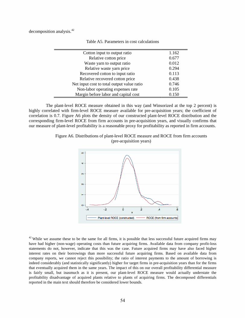
decomposition analysis.42

Table A5. Parameters in cost calculations

Cotton input to output ratio 1.162 Relative cotton price 0.677

Waste yarn to output ratio 0.012 Relative waste yarn price 0.294

Recovered cotton to input ratio 0.113 Relative recovered cotton price 0.438

Net input cost to total output value ratio 0.746 Non-labor operating expenses rate 0.105

Margin before labor and capital cost 0.150

The plant-level ROCE measure obtained in this way (and Winsorized at the top 2 percent) is highly correlated with firm-level ROCE measure available for pre-acquisition years; the coefficient of correlation is 0.7. Figure A6 plots the density of our constructed plant-level ROCE distribution and the corresponding firm-level ROCE from firm accounts in pre-acquisition years, and visually confirms that our measure of plant-level profitability is a reasonable proxy for profitability as reported in firm accounts.

Figure A6. Distributions of plant-level ROCE measure and ROCE from firm accounts (pre-acquisition years)

42 While we assume these to be the same for all firms, it is possible that less successful future acquired firms may have had higher (non-wage) operating costs than future acquiring firms. Available data from company profit-loss statements do not, however, indicate that this was the case. Future acquired firms may have also faced higher interest rates on their borrowings than more successful future acquiring firms. Based on available data from company reports, we cannot reject this possibility; the ratio of interest payments to the amount of borrowing is indeed considerably (and statistically significantly) higher for target firms in pre-acquisition years than for the firms that eventually acquired them in the same years. The impact of this on our overall profitability differential measure is fairly small, but inasmuch as it is present, our plant-level ROCE measure would actually understate the profitability disadvantage of acquired plants relative to plants of acquiring firms. The decomposed differentials reported in the main text should therefore be considered lower bounds.

54

F. Robustness Checks

In this section we describe the details of the design and the results of robustness checks summarized in Section 4.6 of the main text.

We are interested in estimating the following parameters: 𝛽1 = 1

𝑁𝑀∑ � 1

#𝑚𝑖∑ 𝜔𝑗�𝑦𝑗𝑎𝐶 − 𝑦𝑗𝑏𝐶 �𝑗∈𝑚𝑖 �𝑖∈𝑀 , (A1)

𝛽2 = 1𝑁𝑀

∑ �𝑦𝑖𝑏𝐴 −1

#𝑚𝑖𝜔𝑗 ∑ 𝑦𝑗𝑏𝐶𝑗∈𝑚𝑖 �𝑖∈𝑀 , (A2)

𝛽3 = 1𝑁𝑀

∑ ��𝑦𝑖𝑎𝐴 − 𝑦𝑖𝑏𝐴 � −1

#𝑚𝑖∑ 𝜔𝑗�𝑦𝑗𝑎𝐶 − 𝑦𝑗𝑏𝐶 �𝑗∈𝑚𝑖 �𝑖∈𝑀 , (A3)

where M is a set of matches, and acquired plant i is matched with “comparison” plants to form match mi. Outcome variables 𝑦𝑖𝑏𝐴 are TFPQ and ROCE of acquired plant i before an acquisition event, and outcome variables 𝑦𝑗𝑏𝐴 are these variables after the acquisition event. Superscript C indicates the corresponding variables for comparison plants. 𝑁𝑀 is the total number of matches, #𝑚𝑖 is the number of comparison plants within match 𝑚𝑖, and 𝜔𝑗 is a weight attached to the outcome variables, 𝑦𝑗𝑎𝐶 and 𝑦𝑗𝑏𝐶 .

The parameters 𝛽1, 𝛽2 and 𝛽3 can be estimated by 𝑦�𝑖𝑡 = 𝛼0 + 𝛽1𝐴𝐴𝑖𝑡 + 𝛽2𝐴𝑐𝑞𝑢𝑖𝑟𝑒𝑑𝑖𝑡 + 𝛽3𝐴𝑐𝑞𝑢𝑖𝑟𝑒𝑑𝑖 × 𝐴𝐴𝑖𝑡 + 𝜇𝑡 + 𝜀𝑖𝑡, (A4)

where 𝑦�𝑖𝑡 is the outcome variable of plant i at time t if it belongs to a group of acquired plants. The outcome variables of comparison plants within the match 𝑚𝑖 are collapsed to 𝑦�𝑖𝑡 = ∑ 𝜔𝑗𝑦𝑗𝑗∈𝑚𝑖 , the weighted average of outcomes of comparison plants within the match 𝑚𝑖. The variable AAit is a dummy equal to 1 if acquisition mi happened prior to year t and zero otherwise, while the variable Acquiredi is equal to 1 if plant i is purchased in acquisition case mi and zero otherwise. µt is an acquisition-year fixed effect. The estimate �̂�3 reflects the post-acquisition difference-in-difference between acquired and incumbent plants of acquiring firms by accounting for acquisition-case effects.

F.1 Alternative TFPQ measures

In the main text, we used TFPQ estimates obtained from a variant of the De Loecker (2013) method where the production function is approximated by a cubic polynomial. Here we report the results of a robustness check that uses TFPQ values obtained from four alternative production function estimation methods.

The first alternative measure uses De Loecker’s approach but assumes the productivity control function 𝑔(𝜔𝑖𝑡 ,𝑎𝑐𝑞𝑖𝑡) is linear with respect to 𝜔𝑖𝑡. That is,

𝑔(𝜔𝑖𝑡 ,𝑎𝑐𝑞𝑖𝑡) = 𝛾𝑗𝜔𝑖𝑡 + 𝜃1𝑙𝑏_𝑎𝑐𝑞𝑖𝑡 + 𝜃2𝑒𝑎_𝑎𝑐𝑞𝑖𝑡 + 𝜃3𝑙𝑎_𝑎𝑐𝑞𝑖𝑡. In the second measure, 𝑔(𝜔𝑖𝑡,𝑎𝑐𝑞𝑖𝑡) is specified semi-parametrically by including interaction terms between productivity and acquisition-related timing dummies. The third measure of TFPQ is the residuals from the simple OLS regression of the production function. The fourth approach follows the system GMM approach of Blundell and Bond (1998). Here, we do the two-step implementation of the Blundell and Bond estimator with two-period lags, treating the number of worker- and spindle-days as endogenous variables alongside with output, and generating GMM-style instruments for them. All these alternative approaches follow the main specifications in that they include year dummies, the change in log plant capacity from the previous year, and (logged) age of the plant’s machines as additional variables.

F.2 Within-acquired plants estimations

Table A6 presents the results of estimating within-acquired plants effects of Table 2 using the four alternative TFPQ measures. The two De Loecker method specifications produce results that are almost exactly the same as in the main text. Estimations using residuals from the OLS regression and using Blundell and Bond method (with two lags) lead to somewhat lower estimated effects of acquisitions on productivity, especially in the short run. This is entirely consistent with the fact that the De Loecker

55

method is designed to correct for the fact that inputs may change systematically with events that shift productivity levels (acquisitions in our case). If input use rises during acquisition, as we observe in our data, then other approaches may attribute too much of any output growth to input use rather than productivity. That is likely why the OLS and Blundell-Bond approaches find smaller productivity effects immediately after the acquisition. The larger changes observed in the De Loecker estimates avoid this bias. The differences in the estimated TFPQ effects across the methods are smaller in the longer run, however, as much of plants’ post-acquisition input utilization growth has occurred by that point.

Table A6. Within-acquired plants effects of acquisitions––alternative TFPQ methods

All acquisitions Dependent variable: TFPQ

De Loecker OLS Blundell-Bond Linear Non-parametric

Late before acquisition -0.005 -0.004 -0.042 -0.027 (0.018) (0.020) (0.032) (0.033)

Early after acquisition 0.047* 0.049* 0.024 0.025 (0.026) (0.028) (0.042) (0.036)

Late after acquisition 0.126*** 0.130*** 0.103* 0.076 (0.033) (0.036) (0.060) (0.048)

Constant 0.510*** 0.682*** -0.004 0.049 (0.033) (0.035) (0.045) (0.040)

Observations 1,078 1,078 1,151 1,026 Adj. R-squared 0.769 0.772 0.305 0.193

F.3 Same owner matching

We construct two different matched samples to estimate equation (A4). In the first matched sample, which is the one we use in the main text, a match is made based on whether an incumbent plant of an acquiring firm belongs to the same owner who acquired plant i. Thus, comparison plants of acquired plant i are incumbent plants that had been managed by the same owner who acquired the plant i. We call this the “same owner matching” sample.

For this matched sample, we use two different weights to estimate (A4). In the main text, we use a simple weight by setting 𝜔𝑗 = 1 for all j so that all incumbent plants of an acquiring firm carry an equal weight. The other weight first calculates the Mahalanobis distance between an acquired plant and each incumbent plant using plant size, plant age, and plant location. We then generate a weight for an incumbent plant by using this distance and normal kernel. A large weight is assigned to an incumbent plant when it is similar to the acquired plant in terms of these variables.

Tables A7 and A8 report estimation results using this matched sample with different weighting schemes as above. For comparison, we also include results from the standard difference-in-difference estimation where we ignore matching altogether. Table A9 presents the estimation results using different measures of TFPQ as described in Section F.1 and simple weights (results using other types of weights are similar). All specifications include acquisition and calendar year fixed effects, as in the main text.

Tables A7-A9 indicate our results are robust to alternative weights and TFPQ measures.

56

Table A7: Estimation results from same owner matching, all acquisitions

Simple weights Kernel weights Standard DID estimation

TFPQ Plant ROCE TFPQ Plant

ROCE TFPQ Plant ROCE

After acquisition -0.055*** -0.004 -0.050*** -0.005 -0.046*** -0.004 (0.013) (0.012) (0.012) (0.013) (0.010) (0.011)

Acquired plant -0.025 -0.030*** -0.029 -0.038*** -0.032 -0.028*** (0.021) (0.011) (0.022) (0.011) (0.020) (0.009)

After acquisition x Acquired plant

0.091*** 0.040*** 0.074*** 0.038** 0.092*** 0.041*** (0.023) (0.014) (0.022) (0.015) (0.022) (0.013)

Constant 0.480*** 0.145*** 0.462*** 0.144*** 0.471*** 0.143*** (0.034) (0.018) (0.024) (0.018) (0.027) (0.018)

Observations 1,487 1,392 1,208 1,124 1,487 1,392 Note: Robust standard errors clustered at the acquisition-case level in parentheses. *** p<0.01, ** p<0.05, * p<0.1. These symbols apply to all the tables below.

Table A8: Estimation results from same owner matching, serial acquirers

Simple weights Kernel weights Standard DID estimation

TFPQ Plant ROCE TFPQ Plant

ROCE TFPQ Plant ROCE

After acquisition -0.048*** -0.012 -0.049*** -0.019 -0.029*** -0.006 (0.008) (0.016) (0.010) (0.019) (0.006) (0.014)

Acquired plant -0.032* -0.032** -0.035* -0.046*** -0.026 -0.022*

(0.017) (0.013) (0.018) (0.014) (0.017) (0.011)

After acquisition x Acquired plant

0.113*** 0.058*** 0.098*** 0.057** 0.108*** 0.053*** (0.028) (0.017) (0.028) (0.021) (0.029) (0.016)

Constant 0.410*** 0.069*** 0.388*** 0.083*** 0.408*** 0.060*** (0.008) (0.013) (0.018) (0.014) (0.009) (0.011)

Observations 1,067 994 822 764 1,067 994

Table A9: Estimation results from same owner matching, several TFPQ measures

All acquisitions and Simple weights De Loecker OLS Blundell-Bond

Linear Non-parametric After acquisition -0.059*** -0.060*** -0.064** 0.020***

(0.013) (0.014) (0.026) (0.007) Acquired plant -0.030 -0.028 0.009 -0.034***

(0.021) (0.023) (0.028) (0.010) After acquisition x

Acquired plant 0.098*** 0.097*** 0.093*** 0.032** (0.023) (0.024) (0.031) (0.013)

Constant 0.330*** 0.463*** -0.015 0.087*** (0.034) (0.035) (0.123) (0.022)

Observations 1,487 1,487 1,539 1,467

57

F.4 Pre-acquisition characteristics and trend matching

While matching on the same ultimate owner seems to be the most natural procedure in our case, we also created an alternative matched sample to estimate equation (A4) by forming matches based on whether a non-acquired plant is similar to acquired plant i in terms of pre-acquisition characteristics or pre-acquisition trends of outcome variables. To construct this matched sample, we first specify a group of non-acquired plants that could be potentially matched with each acquired plant. Potential non-acquired plants include all those plants that were owned by acquiring firms and were never acquired themselves, but also include plants of firms that did not participate in the acquisition process at all as well as plants that were acquired during the sample but at a time that is sufficiently removed from the event for which they serve as a control.43

We calculate the Mahalanobis distance between a particular acquired plant and each non-acquired plant using two sets of variables. One includes the pre-acquisition plant size, plant age, and plant location. The other set includes average pre-acquisition TFPQ growth and ROCE growth. A small distance value indicates that an acquired plant and a non-acquired plant are similar with respect to pre-acquisition TFPQ and ROCE growth rates. A non-acquired plant is included in a particular match only if its distance is below the median of the overall sample.

44

Tables A10, A11, and A12 present estimation results using this matched sample. Again, the main results are robust to alternative matching criteria and alternative measures of TFPQ.

We use the simple weight (i.e., 𝜔𝑗 = 1) for this estimation.

Table A10: Estimation results from pre characteristics and trend matching, all acquisitions

Matching Criteria

Plant age, size, location TFPQ growth rate Plant ROCE growth rate

TFPQ Plant ROCE TFPQ Plant ROCE After acquisition -0.053*** -0.007 -0.042*** 0.020***

(0.010) (0.007) (0.011) (0.007)

Acquired plant -0.007 -0.029*** 0.009 -0.034***

(0.021) (0.011) (0.026) (0.010)

After acquisition x Acquired plant

0.078*** 0.038*** 0.065** 0.032** (0.024) (0.012) (0.024) (0.013)

Constant 0.332*** 0.039*** 0.402*** 0.087***

(0.021) (0.005) (0.081) (0.022)

Observations 9,680 7,966 8,640 4,687

43 More specifically, acquired plants in 3 years prior to and 5 years after their own acquisition events are excluded. A plant was also excluded when it does not have any usable observations before or after the acquisition event. 44 We used other cutoff values such as the mean and lower quartile for this estimation, and the results remained unchanged qualitatively.

58

Table A11: Estimation results from pre characteristics and trend matching, serial acquirers

Matching criteria

Plant age, size, location TFPQ growth rate Plant ROCE growth rate

TFPQ Plant ROCE TFPQ Plant ROCE After acquisition -0.048*** -0.006 -0.045*** -0.009

(0.009) (0.009) (0.009) (0.010)

Acquired plant 0.019 -0.015 0.030 -0.028*

(0.018) (0.014) (0.032) (0.014)

After acquisition x Acquired plant

0.092*** 0.041*** 0.089** 0.045** (0.031) (0.015) (0.032) (0.017)

Constant 0.329*** 0.039*** 0.292*** 0.065***

(0.006) (0.005) (0.016) (0.014)

Observations 6,197 5,086 5,155 3,050

Table A12: Estimation results from pre characteristics and trend matching, several TFPQ measures

Matching criteria: Plant age, size, location Dependent variable: TFPQ

De Loecker OLS Blundell-Bond Linear Non-parametric

After acquisition -0.054*** -0.057*** -0.052*** -0.036*** (0.010) (0.010) (0.016) (0.012)

Acquired plant -0.005 -0.014 -0.006 0.001 (0.021) (0.023) (0.022) (0.018)

After acquisition x Acquired plant

0.079*** 0.082*** 0.083*** 0.059*** (0.024) (0.025) (0.028) (0.020)

Constant 0.180*** 0.307*** 0.030 -0.004 (0.022) (0.025) (0.110) (0.032)

Observations 9,680 9,680 9,989 9,469

F.5 Placebo test

We also perform a placebo test as a further robustness check. We randomly assign acquisition status to plants in the sample and estimate how the outcome variables are related to this randomly generated acquisition status. Specifically, we use the same-owner matched sample and generate a random variable from the uniform distribution for each plant in the whole matched sample. 45

Table A13 reports the results from this placebo test. The magnitudes of both the acquisition main effect and its interaction with the after-acquisition dummy approach zero and are economically insignificant.

We assign an acquired plant status to a plant that obtained the maximum value within a particular match. We then estimate the parameters of specification (A4) by using all acquisition cases and simple weights. We repeat this procedure 1000 times, and calculate a sample mean of estimated coefficients from these 1000 simulations, and their standard errors.

45 The results are robust to using a pre-characteristics and trend matched samples.

59

Table A13: Placebo test

TFPQ Mean Std. Err 95% Conf. Interval

After acquisition -0.0149 0.0003 -0.0155 -0.0143 Acquired plant -0.0010 0.0006 -0.0023 0.0002 After acquisition x Acquired plant 0.0010 0.0006 -0.0002 0.0022 Constant 0.4666 0.0003 0.4659 0.4672

Plant ROCE Mean Std. Err 95% Conf. Interval

After acquisition 0.0139 0.0002 0.0135 0.0143 Acquired plant 0.0002 0.0003 -0.0005 0.0009 After acquisition x Acquired plant 0.0000 0.0004 -0.0008 0.0008 Constant 0.1364 0.0002 0.1360 0.1368

G. Decline in total input to total asset ratios in later post-acquisition years

As mentioned in the main text, the decline in the input-to-asset ratio in the late post-acquisition period (see Table 5) is not a result of less utilization of available physical plant capacity. It instead reflects a sharp increase in total assets due to retained earnings. Table 5 indicates the ratio of physical plant capacity to those total assets that declines in late post-acquisition years, not physical capacity utilization rates. To see this more clearly, in Table A14 we further decompose the logged ratio of physical plant capacity to total assets from Table 5 into the sum of (logged) ratio of total input to plant (spindle) capacity, and the (logged) ratio of plant spindle capacity to total capital employed.

We can see from Table A14 that the six-percent drop in the total input to capital employed ratio from early to late post-acquisition period is entirely accounted for by the drop in the ratio of plant capacity to capital employed ratio. To explore this issue more deeply, we looked at changes in the composition of balance sheets of acquiring firms in our sample.

Figure A7 shows that starting in the middle of the 20th century’s first decade, there is a sharp increase in the share of reserves (retained earnings) on the debit side of the balance sheets of major acquiring firms. Correspondingly, there is also a pronounced decline in the share of fixed assets (land, buildings, machines and other equipment) in total assets on the credit side, compensated by higher liquidity in banking accounts as well as oftentimes large amounts of funds tied up in “production facilities expansion accounts” (that is, new fixed assets yet to be installed). As shown in Figure A1 above, capacity expansion which had been on hold for the first 8-10 years of our sample resumed towards the end of the first decade of the 20th century. Thus the decline in existing plants’ capacity in the total assets amassed by acquiring firms simply reflects their rapid expansion (building of new plants and expanding old ones) financed mostly through accumulated retained earnings. Since late post-acquisition years in our sample coincide with this expansion period, decomposition results create an appearance of reduced capacity utilization towards later post-acquisition period. However, this does not mean that existing physical capacity of acquired plants was once again underutilized. In fact, directly measured capacity utilization rates (ratios of spindle-days in operation to total number of installed spindles, times 365) increase by 7.5 percent from pre- to early post-acquisition period and by 9.3 percent from pre- to late post-acquisition period, with both differences statistically significant at 1 percent level. These differentials are considerably higher than the total input/plant capacity ratio differentials in Table A14, and closely correspond to the differentials between our TFPQU and TFPQ measures reported in Table 6.

60

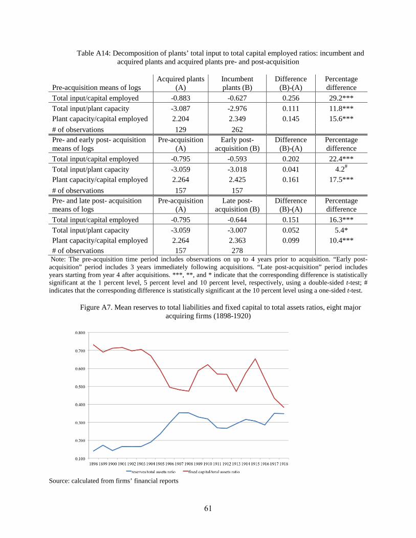
Table A14: Decomposition of plants’ total input to total capital employed ratios: incumbent and acquired plants and acquired plants pre- and post-acquisition

Pre-acquisition means of logs Acquired plants

(A) Incumbent plants (B)

Difference (B)-(A)

Percentage difference

Total input/capital employed -0.883 -0.627 0.256 29.2*** Total input/plant capacity -3.087 -2.976 0.111 11.8*** Plant capacity/capital employed 2.204 2.349 0.145 15.6*** # of observations 129 262 Pre- and early post- acquisition means of logs

Pre-acquisition (A)

Early post-acquisition (B)

Difference (B)-(A)

Percentage difference

Total input/capital employed -0.795 -0.593 0.202 22.4*** Total input/plant capacity -3.059 -3.018 0.041 4.2#

Plant capacity/capital employed 2.264 2.425 0.161 17.5*** # of observations 157 157 Pre- and late post- acquisition means of logs

Pre-acquisition (A)

Late post-acquisition (B)

Difference (B)-(A)

Percentage difference

Total input/capital employed -0.795 -0.644 0.151 16.3*** Total input/plant capacity -3.059 -3.007 0.052 5.4* Plant capacity/capital employed 2.264 2.363 0.099 10.4*** # of observations 157 278

Note: The pre-acquisition time period includes observations on up to 4 years prior to acquisition. “Early post- acquisition” period includes 3 years immediately following acquisitions. “Late post-acquisition” period includes years starting from year 4 after acquisitions. ***, **, and * indicate that the corresponding difference is statistically significant at the 1 percent level, 5 percent level and 10 percent level, respectively, using a double-sided t-test; # indicates that the corresponding difference is statistically significant at the 10 percent level using a one-sided t-test.

Figure A7. Mean reserves to total liabilities and fixed capital to total assets ratios, eight major acquiring firms (1898-1920)

Source: calculated from firms’ financial reports

61

H. In- and out-of-network firms distribution densities of ROCE, unrealized output rates, capacity utilization and prices

Figures A8-A13 show the full density distributions of in- and out-of network firm characteristics, the means for which are presented in Table 8 in the main text.

Figure A8. TFPQ, 1898-1902

Figure A9. TFPQU, 1898-1902

62

Figure A10. Return on capital employed, 1898-1902

Figure A11. Unrealized output to produced output ratios, 1898-1902

63

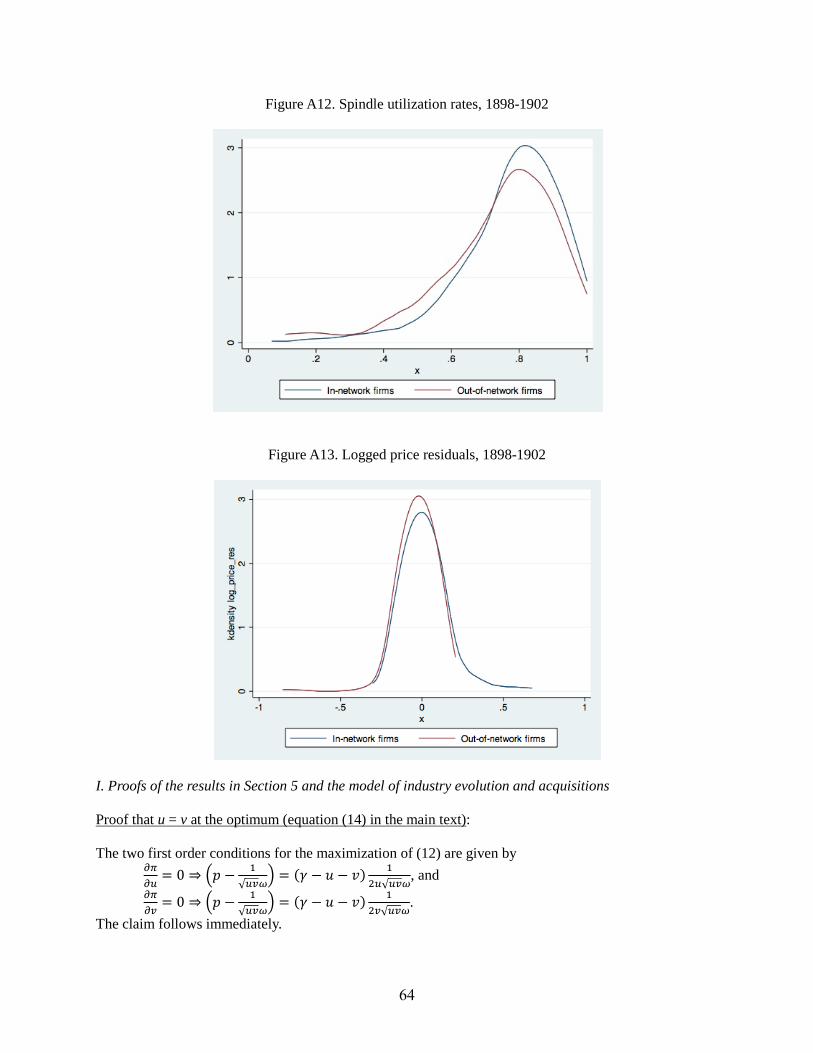
Figure A12. Spindle utilization rates, 1898-1902

Figure A13. Logged price residuals, 1898-1902

I. Proofs of the results in Section 5 and the model of industry evolution and acquisitions

Proof that u = v at the optimum (equation (14) in the main text):

The two first order conditions for the maximization of (12) are given by 𝜕𝜋𝜕𝑢

= 0 ⇒ �𝑝 − 1√𝑢𝑣𝜔

� = (𝛾 − 𝑢 − 𝑣) 12𝑢√𝑢𝑣𝜔

, and 𝜕𝜋𝜕𝑣

= 0 ⇒ �𝑝 − 1√𝑢𝑣𝜔

� = (𝛾 − 𝑢 − 𝑣) 12𝑣√𝑢𝑣𝜔

. The claim follows immediately.

64

Proof of Lemma 1(i): Straightforward from (10) and (12) in the main text.

Proof of Lemma 1(ii):

We have

𝜋(𝛾,𝜔) = 𝑝𝛾 + 2𝜔− 2�2𝑝𝛾

𝜔.

𝜕𝜋(𝛾,𝜔)𝜕𝛾

= 𝑝𝛾�𝛾 − �2𝛾

𝑝𝜔� = 𝑝

𝛾(𝛾 −𝑚) > 0.

𝜕𝜋(𝛾,𝜔)𝜕𝜔

= 𝑚𝜔��2𝑝𝛾

𝜔1𝑚− 2

𝜔𝑚� = 𝑚

𝜔�𝑝 − 2

𝜔𝑚� > 0.

The first two claims follow immediately. Also, 𝑥∗ = 2(𝛾−𝑚)𝑚𝜔

= �2𝛾𝑝𝜔− 1

𝜔, which is also clearly increasing

in 𝛾.

Proof of Lemma 1(iii):

We have 𝜕2𝜋(𝛾,𝜔)𝜕𝛾𝜕𝜔

= �𝑝

2𝛾𝜔3 > 0.

Details of the model in Section 5.3:

Stage I Each first-cohort entrant is endowed with some initial level of demand management ability, 𝛾0

(and a plant of quality 𝜔1). Given a fixed (flow) operation cost, 𝑓, and a demand structure 𝐷(𝑝), free entry implies that the number (mass) of first-cohort entrants, 𝑁1, and the initial equilibrium price 𝑝0, will be determined by the following two equations comprised of the market-clearing and the free-entry zero-profit conditions:

𝐷(𝑝0) = [𝛾0 − 𝑚(𝛾0𝜔1;𝑝0)]𝑁1 = �𝛾0 − �2𝛾0 𝑝0𝜔1⁄ �𝑁1, 𝜋(𝛾0,𝜔1;𝑝0) = 𝑓. We assume that during Stage I some first-cohort entrants obtain a management ability level above

𝛾0 (for instance, they make connections with traders or are able to hire an educated engineer). Thus, at the end of Stage I, the first cohort’s ability is distributed with support [𝛾0, 𝛾𝑚𝑎𝑥]. An equilibrium at the end of Stage I would thus be characterized by a price 𝑝∗ and a threshold ability level 𝛾∗ > 𝛾0, that satisfy the following market-clearing and zero-profit conditions:

𝐷(𝑝∗) = ∫ �𝛾 − �2𝛾 𝑝𝜔1⁄ �𝛾𝑚𝑎𝑥𝛾∗ 𝑑𝐹(𝛾), (A5)

𝜋(𝛾∗,𝜔1;𝑝∗) = 𝑓, or 𝛾∗ = ��𝑓𝜔1 + √2�2𝑝∗𝜔1� (A6)

Stage II At this stage, the refinement arrives but each firm can still only manage one plant (its original one

for first-cohort entrants). Assume that the size of the “refinement” (the jump from 𝜔1 to 𝜔2) is high enough to justify new entry under the previous equilibrium (A5)-(A6) (that is, that 𝜋(𝛾0,𝜔2;𝑝∗) >𝜋(𝛾∗,𝜔1;𝑝∗) = 𝑓). As the second-cohort firms enter, the equilibrium price starts falling until a new industry equilibrium is reached, characterized by (i) the new market clearing condition (where 𝑁2 is the total mass of the second cohort entrants):

𝐷(𝑝∗∗) = ∫ �𝛾 − �2𝛾 𝑝∗∗𝜔1⁄ �𝛾𝑚𝑎𝑥𝛾∗∗ 𝑑𝐹(𝛾) + 𝑁2�𝛾0 − �2𝛾0 𝑝∗∗𝜔2⁄ �, (A7)

(ii) zero-profit condition for the first cohort:

65

𝜋(𝛾∗∗,𝜔1;𝑝∗∗) = 𝑓, or 𝛾∗∗ = ��𝑓𝜔1 + √2�2𝑝∗∗𝜔1� , (A8)

and (iii) zero-profit condition for the second cohort: 𝜋(𝛾0,𝜔2;𝑝∗∗) = 𝑓 or 𝛾0 = ��𝑓𝜔2 + √2�

2𝑝∗∗𝜔2� . (A9)

These three conditions jointly determine the new equilibrium price 𝑝∗∗, the cutoff ability of remaining first-cohort entrants 𝛾∗∗, and the mass of second-cohort entrants, 𝑁2 . Comparing conditions (A7) and (A5), we see that 𝑝∗∗ < 𝑝∗ implies 𝛾∗∗ > 𝛾∗, so that only first-cohort plant owners whose ability exceeds a threshold level 𝛾∗∗ ∈ (𝛾∗, 𝛾𝑚𝑎𝑥) can remain in the industry; those below it exit. To make things interesting (and correspond to the specifics of the industry), we also assume that 𝛾∗∗ < 𝛾𝑚𝑎𝑥. That is, the mass of remaining first-cohort entrants is non-degenerate (and actually is large enough in a sense made more precise below).

Stage III The third stage is a merger and acquisition stage where physical assets are exchanged. To ease

notation, we assume that each firm can buy at most one plant in the market for physical assets. (An extension where it can buy more than one plant is straightforward.) We assume as in Jovanovic and Braguinsky (2004) that assets (plants) are simply bought and sold in the market for a given price. In reality, of course, most acquisition deals are negotiated bilaterally. Available evidence from our sample (the qualitative descriptions of acquisition deals in, e.g., Kinugawa, 1964, as well as in company histories) suggests, however, that all such deals involved both acquirers’ and targets’ shareholders meetings debating the terms, sometimes comparing multiple offers and occasionally rejecting proposed deals and deciding to continue soldiering on alone or seek another acquirer (target). In many cases, the parties involved in a deal were also brought together by prominent mediators (including those from major trading houses), with good knowledge of the market environment. The detailed operations and financial data which we use in this paper, and which were in open access already at that time, also made it easier to estimate a plant’s fair market price. Hence, assuming that acquisition deals were consummated at a market price does not seem to be that far removed from how those deals actually happened in our sample.

Let the price of a plant of quality 𝜔𝑖 be given by 𝑠𝜔𝑖 , 𝑖 = 1,2. A firm will sell its plant if

𝑠𝜔𝑖 − 𝜋(𝛾,𝜔𝑖; 𝑝) + 𝑓 ≥ 0 or ��𝜔𝑖�𝑠𝜔𝑖+𝑓�+√2�

2

𝑝𝜔𝑖≥ 𝛾. (A10)

Since there is no variation in 𝛾 for the second-cohort firms, given price 𝑠𝜔2, all their plants are offered for sale in Stage III as long as

��𝜔2�𝑠𝜔2+𝑓�+√2�2

𝑝𝜔2≥ 𝛾0. (A11)

The aggregate supply of plants with quality 𝜔2 is given by 𝑄𝜔2�𝑠𝜔2 ,𝑝� = 𝑁2 (A12)

if condition (A11) is met. It is easy to see that this condition will be met in any equilibrium, as there is value created by reallocating a plant of quality 𝜔2 from its second-stage owner to a first-cohort firm. Thus condition (A11) simply implies that price 𝑠𝜔2 should be high enough to induce those plant owners to sell. In what follows we also assume there is enough demand from higher-ability owners for 𝜔2-type plants to induce a high enough price such that inequality (A11) is strict. (In particular, this will always be the case if we relax the assumption that a firm can buy at most one plant.)46

46 If the parameters of the model are such that the total mass of first-cohort firms remaining in the industry is less than 𝑁2 (the mass of second-cohort entrants), there will be not enough demand for second-cohort plants, pushing the price 𝑠𝜔2 all the way down until condition (A11) is met with equality. (In this situation, owners of second-cohort plants will be indifferent between selling and operating, so some will sell their plants and exit the industry, while others will keep operating their plants. There will be no market for plants of 𝜔1 quality in this case.) While we cannot rule out such a situation on a priori grounds, it does not fit the industry specifics.

The total supply of such plants is thus

66

fixed and given by 𝑁2, while price 𝑠𝜔2 is determined solely by the demand side (discussed below). The aggregate supply of plants with quality 𝜔1, on the other hand, is given by 𝑄𝜔1�𝑠𝜔1 ,𝑝� = ∫ 𝑑𝐹(𝛾)𝛾�

𝛾∗∗ , (A13) where 𝛾� is the ability level where condition (A10) is met with equality (for 𝑖 = 1). As we can see, 𝑄𝜔1�𝑠𝜔1 ,𝑝� is an increasing function of 𝑠𝜔1. The ability of the marginal seller, 𝛾�, is also increasing in 𝑠𝜔1.

We turn now to the demand for plants. A firm buys a plant of quality 𝜔𝑖 if its profit, net of purchasing price and operating cost, is positive:

𝜋(𝛾,𝜔𝑖;𝑝) − 𝑓 > 𝑠𝜔𝑖. (A14) Note that since ability 𝛾 and plant quality 𝜔 are complements in the profit function (Lemma 1 in the main text), the demand for higher-quality (𝜔2 -type) plants comes entirely from the top of the ability distribution 𝛾 . This complementarity makes sure that in equilibrium, the price 𝑠𝜔2 will “ration” the demand for second-cohort plants to just the first 𝑁2 highest-ability firms. Hence, this demand is given by

𝑋𝜔2�𝑠𝜔2 ,𝑝� = ∫ 𝑑𝐹(𝛾)𝛾𝑚𝑎𝑥𝛾𝑁2

, (A15)

where 𝛾𝑁2 satisfies the condition under which the buyer with ability 𝛾𝑁2 is just indifferent between buying plants of either quality:

𝜋�𝛾𝑁2 ,𝜔2;𝑝� − 𝜋�𝛾𝑁2 ,𝜔1;𝑝� = 𝑠𝜔2 − 𝑠𝜔1. (A16) The remaining first-cohort entrants then reallocate their 𝜔1 -type plants among themselves. More specifically, the demand for plants with quality 𝜔1 is given by

𝑋𝜔1�𝑠𝜔1 ,𝑝� = ∫ 𝑑𝐹(𝛾)𝛾𝑁2𝛾� , (A17)

where 𝛾� is as in (A13). As we can see, 𝑋𝜔1�𝑠𝜔1 ,𝑝� is a decreasing function of 𝑠𝜔1. To close the system, we need the output market clearing condition: 𝐷(�̂�) = ∫ �𝛾 − �2𝛾 �̂�𝜔1⁄ �𝛾𝑚𝑎𝑥

𝛾� 𝑑𝐹(𝛾)

+∫ �𝛾 − �2𝛾 �̂�𝜔1⁄ �𝛾𝑁2𝛾� 𝑑𝐹(𝛾) + ∫ �𝛾 − �2𝛾 �̂�𝜔2⁄ �𝛾𝑚𝑎𝑥

𝛾𝑁2𝑑𝐹(𝛾), (A18)

where the first term on the right-hand side is the supply of incumbent plants of all the remaining firms, the second term is the supply of newly acquired 𝜔1-type plants, and the third term is the supply of newly acquired 𝜔2-type plants. Together, the output market clearing condition (A18), the two conditions that clear the markets for 𝜔1-type plants and 𝜔2-type plants (namely, that (A13) and (A17) equal one another and that (A15) is equal to 𝑁2), along with two indifference conditions for marginal buyers of 𝜔1-type plants ((A10) with equality for 𝑖 = 1) and of 𝜔2-type plants (A16), pin down the equilibrium quintuple of prices and cutoff ability levels ��̂�, �̂�𝜔1 , �̂�𝜔2 ,𝛾�, 𝛾𝑁2�. 47 One important feature is that high-ability early entrants with aged plants acquire more recent entrants with lower ability management but newer plants.

Proof of Proposition 2:

We show that 𝜕𝑙𝑛[𝜋(𝜔,𝛾)]𝜕𝛾

> 𝜕𝑙𝑛[𝑇𝐹𝑃𝑄]𝜕𝛾

for any given 𝜔. We have:

𝑙𝑛[𝜋(𝜔, 𝛾)] = 𝑙𝑛 �𝑝𝛾 + 2𝜔− 2�2𝑝𝛾

𝜔�.

Differentiating with respect to 𝛾 yields

47 The proof of existence, uniqueness (under suitable parametric restrictions) and (constrained) optimality parallels closely the proof of Proposition 2 in Jovanovic and Braguinsky (2004), so we do not reproduce it here. In the model here, the equilibrium in Stage III involves all firms participating in the acquisitions market. Jovanovic and Braguinsky (2004) introduce a fixed cost of acquisition (“due diligence”), which makes sure that there are firms that do not participate in the acquisition markets as either buyers or sellers. Such firms exist in our data too, and a fixed cost of acquisition would account for this feature here as well (details are available upon request).

67

𝜕𝑙𝑛[𝜋(𝜔,𝛾)]𝜕𝛾

=𝑝−1𝛾�

2𝑝𝛾𝜔

𝜋.

Also, 𝑙𝑛[𝑇𝐹𝑃𝑄] = 1

2𝑙𝑛 �𝛾𝜔

2𝑝�.

Differentiating with respect to 𝛾 yields 𝜕𝑙𝑛[𝑇𝐹𝑃𝑄]

𝜕𝛾= 1

2𝛾.

Comparing the two,

𝜕𝑙𝑛[𝜋(𝜔,𝛾)]𝜕𝛾

− 𝜕𝑙𝑛[𝑇𝐹𝑃𝑄]𝜕𝛾

=𝑝𝛾+�2𝑝𝛾𝜔 −2

𝜔

2𝜋𝛾= 𝑝𝛾𝜔−2+�2𝑝𝛾𝜔

2𝜔𝜋𝛾> 0,

because 𝑝𝛾𝜔 − 2 = ��𝑝𝛾𝜔 + √2���𝑝𝛾𝜔 − √2� > 0 by (13) in the main text.

Proof of Proposition 3:

Let subscripts A and T denote acquiring and target plants, respectively. The TFPQ difference between the acquiring and the target plants is given by

�𝛾𝐴𝜔𝐴2𝑝

− �𝛾𝑇𝜔𝑇2𝑝

. (A19)

The difference in profits between the acquiring and target plants, on the other hand, is given by

�𝑝𝛾𝐴 + 2𝜔𝐴

− 2�2𝑝𝛾𝐴𝜔𝐴

� − �𝑝𝛾𝑇 + 2𝜔𝑇− 2�2𝑝𝛾𝑇

𝜔𝑇�

= 𝑝(𝛾𝐴 − 𝛾𝑇) + � 2𝜔𝐴

− 2𝜔𝑇� − 2 ��2𝑝𝛾𝐴

𝜔𝐴− �2𝑝𝛾𝑇

𝜔𝑇�

= 𝑝(𝛾𝐴 − 𝛾𝑇) + 2� 1𝜔𝐴�1 −�2𝑝𝛾𝐴𝜔𝐴� −

1𝜔𝑇�1 −�2𝑝𝛾𝑇𝜔𝑇��. (A20)

Assume now that the difference in (A19) above is zero. This means that the difference (A20) boils down to

𝑝(𝛾𝐴 − 𝛾𝑇) + 2 � 1𝜔𝐴

− 1𝜔𝑇� > 0,

which is positive because 𝛾𝐴 > 𝛾𝑇 , while 𝜔𝑇 > 𝜔𝐴 by the assumption that the target plant has higher quality. We have thus shown that if the TFPQ of the acquiring and target plants are the same, the profit of the acquiring firm will be higher than the profit of the target firm (this also follows directly from Proposition 2, of course). By continuity, the profit of the acquiring firm will still be higher than that of the target firm even for some range of parameters where TFPQ(acquirer) < TFPQ(target). It is also clear from the expression above that this range will be larger when the difference 𝛾𝐴 − 𝛾𝑇 is larger.

J. Numerical Example of the Model

Set the value of model’s parameters as follows: 𝑝 = 3,𝜔𝑒𝑛𝑡𝑟𝑎𝑛𝑡 = 1.5,𝜔𝑖𝑛𝑐𝑢𝑚𝑏𝑒𝑛𝑡 = 1, 𝛾0 = 2. Assume that surviving incumbents’ ability, 𝛾𝑖𝑛𝑐𝑢𝑚𝑏𝑒𝑛𝑡, is uniformly distributed over the interval [2.45, 3.5]. The choice of the lower bound for 𝛾𝑖𝑛𝑐𝑢𝑚𝑏𝑒𝑛𝑡 ensures that the lowest-ability incumbent attains the same profits as all entrants, while the upper bound gives the highest-ability incumbent profits that are twice as large as entrants’ profits.

Under these parameters, the optimal choice of m, the maximized profit, input utilization and TFPQ are given by the values in Table A15 below.

68

Table A15. Numerical example: New entrant, low- and high-ability incumbents

New entrant Low-ability incumbent High-ability incumbent Time managing production 0.94 1.28 1.53

Total input 1.50 1.83 2.58 Input utilization 0.69 0.80 0.87

TFPQ 1.03 0.80 0.87 Profit 1.68 1.68 3.33

Profit/total input 1.12 0.92 1.29

As can be seen from Table A15, high-ability incumbent’s profit is double the profit of both new entrant and low-ability incumbent, but its TFPQ is lower than that of a new entrant. Input utilization is the lowest for a new entrant, higher for a low-ability incumbent, and highest for the high-ability incumbent. These are exactly the patterns we saw in the data.

What happens after a high-ability incumbent acquires a new entrant or a low-ability incumbent in the setup above? Recalculating optimal m using the acquirer’s ability level 𝛾 = 3.5 yields the changes presented in Table A16 below.

Table A16. Numerical example: New entrant and low-ability incumbent from before to after acquisition by a high-ability incumbent

New entrant Low-ability incumbent Pre-acquisition Post-acquisition Pre-acquisition Post-acquisition

Time managing production 0.94 1.25 1.28 1.53 Total input 1.50 2.41 1.83 2.58

Input utilization 0.69 0.79 0.80 0.87 TFPQ 1.03 1.18 0.80 0.87 Profit 1.68 4.35 1.68 3.33

Profit/total input 1.12 1.81 0.92 1.29

Under the new, more capable ownership, plants of both new entrants and low-ability incumbents improve input utilization and TFPQ. Profits jump by even more; they double for the low-ability incumbent plant from before to after acquisition, and increase 2.6 times over for the plant formerly owned by a new entrant. Even when normalized by total input, the profit rate improves by more than TFPQ, again consistent with the patterns we discovered in our sample.

K. Year-by-year estimates of within-acquisition comparisons between incumbent and acquired plants

We first estimate TFPQ and TFPQU regressions similar to (5) with a full set of annual pre- and post-acquisition year dummies. The year-by-year coefficients for TFPQ and TFPQU and the difference between them are plotted in Figure A14 along with the corresponding 95-percent confidence intervals (using robust standard errors clustered at the acquisition level). There is no discernible pre-acquisition trend in either TFPQ or TFPQU, while there is a clear upward trend in both after acquisitions. Moreover, TFPQU jumps up immediately after the acquisition event, while TFPQ grows more slowly. The difference between the two thus stays more or less constant for much of the post-acquisition period, indicating that capacity utilization improves almost instantaneously following acquisition and then grows relatively slowly, with lion’s share of the improvement in plant productivity in later years coming from TFPQ (more efficient use of capital and labor flows conditioning on operating).

69

Figure A14. TFPQ and TFPQU dynamics of acquired plants

Note: The horizontal axis represents time to and after acquisition events, with year 0 being the acquisition year. The graph plots coefficients on each pre- and post-acquisition year dummies estimated using equation (5) with the full set of pre-acquisition and post-acquisition dummies, excluding the acquisition year itself. Years 10 and earlier before acquisition event and years 10 and later after acquisition events are collapsed into a single dummy. The omitted category is 10 years or more before acquisition. Error bars display 95 percent confidence intervals.

Figure A15 presents the results of TFPQ estimated by the “difference-in-difference” estimation equation (6) in the main text, also with a full set of yearly time dummies (the results for TFPQU are similar):

𝑦�𝑖𝑡 = 𝛼0 + ∑ 𝛽𝑠𝐼𝑛𝑐𝚤𝑠������8𝑡=𝑇−4,𝑡≠𝑜 + ∑ 𝛽𝑠𝐴𝑐𝑞𝑖𝑠8

𝑡=𝑇−4 + 𝑚𝑖𝑡 + 𝜀𝑖𝑡 , (A21)

where, as in the main text, 𝑦�𝑖𝑡 is TFPQ (relative to industry-year average) of plant i at time t if it is an acquired plant, while TFPQs (also relative to industry-year average) of incumbent plants are collapsed to 𝑦�𝑖𝑡 = 1

#𝑚𝐴∑ 𝑦𝑗𝑡𝑗∈𝑚𝐴 , where 𝑚𝐴 denotes the particular acquisition case in which plant i was acquired and

#𝑚𝐴 is the number of incumbent plants in acquisition 𝑚𝐴. The timeline is, once again, from 4 years before to 8 years after acquisitions. (The omitted category is TFPQ of incumbent plants in the year of acquisition, so all other variables are measured relative to the incumbent plants’ average TFPQ in the acquisition year.)

Consistent with the results in Table 3 in the main text, TFPQ of acquired plants is somewhat higher than TFPQ of incumbent plants before acquisition, but the difference is not statistically significant. There is no particularly pronounced trend in incumbent or acquired plants’ TFPQ before acquisition. After acquisition, however, acquired plants clearly diverge upward from incumbent plants (and the rest of the industry––recall that TFPQ are the residuals from production function estimates using all available data for all years, including also year dummies).

70

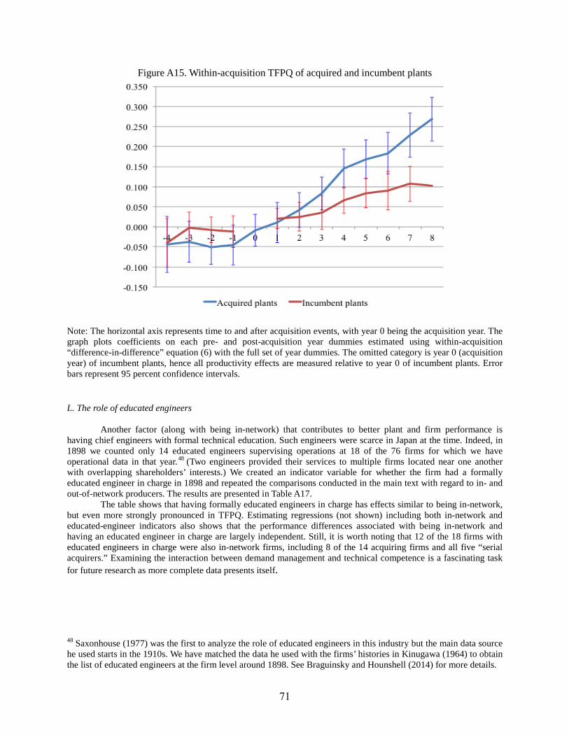
Figure A15. Within-acquisition TFPQ of acquired and incumbent plants

Note: The horizontal axis represents time to and after acquisition events, with year 0 being the acquisition year. The graph plots coefficients on each pre- and post-acquisition year dummies estimated using within-acquisition “difference-in-difference” equation (6) with the full set of year dummies. The omitted category is year 0 (acquisition year) of incumbent plants, hence all productivity effects are measured relative to year 0 of incumbent plants. Error bars represent 95 percent confidence intervals.

L. The role of educated engineers

Another factor (along with being in-network) that contributes to better plant and firm performance is having chief engineers with formal technical education. Such engineers were scarce in Japan at the time. Indeed, in 1898 we counted only 14 educated engineers supervising operations at 18 of the 76 firms for which we have operational data in that year.48

The table shows that having formally educated engineers in charge has effects similar to being in-network, but even more strongly pronounced in TFPQ. Estimating regressions (not shown) including both in-network and educated-engineer indicators also shows that the performance differences associated with being in-network and having an educated engineer in charge are largely independent. Still, it is worth noting that 12 of the 18 firms with educated engineers in charge were also in-network firms, including 8 of the 14 acquiring firms and all five “serial acquirers.” Examining the interaction between demand management and technical competence is a fascinating task for future research as more complete data presents itself.

(Two engineers provided their services to multiple firms located near one another with overlapping shareholders’ interests.) We created an indicator variable for whether the firm had a formally educated engineer in charge in 1898 and repeated the comparisons conducted in the main text with regard to in- and out-of-network producers. The results are presented in Table A17.

48 Saxonhouse (1977) was the first to analyze the role of educated engineers in this industry but the main data source he used starts in the 1910s. We have matched the data he used with the firms’ histories in Kinugawa (1964) to obtain the list of educated engineers at the firm level around 1898. See Braguinsky and Hounshell (2014) for more details.

71

Table A17. Plant and firm performance metrics in 1898-1902 by firms with and without educated engineers

Outcome No formally educated engineer (A)

Formally educated engineer (B) Difference (B-A)

TFPQ 0.435 0.517 0.082*** TFPQU 0.131 0.286 0.156*** ROCE 0.024 0.072 0.047***

Unrealized output ratios 0.119 0.077 -0.042*** Spindle utilization rates 0.746 0.792 0.046*** Logged price residuals -0.014 0.021 0.035**

# of observations 188 109 Note: *** and ** indicate that the corresponding difference is statistically significant at the 1 percent level and 5 percent level, respectively, using a double-sided t-test.

Appendix References

Klepper, Steven and Kenneth L. Simons, 2000. “Dominance by Birthright: Entry of Prior Radio Producers and Competitive Ramifications in the U.S. Television Receiver Industry,” Strategic Management Journal, 21 (10-11), 997-1016.

Otsuka, Keijiro, Gustav Ranis, and Gary Saxonhouse, 1988. Comparative Technology Choice in Development: the Indian and Japanese Cotton Textile Industries. Basingstoke: McMillan.

Wright, Gavin, 2011. Cotton Spinning Machinery Orders, British Textile Machinery Firms, 1878-1933. ICPSR27141-v1. Ann Arbor, MI: Inter-university Consortium for Political and Social Research [distributor], 2011-11-18. doi:10.3886/ICPSR27141.v1.

72

NBB WORKING PAPER No. 270 – OCTOBER 2014 73

NATIONAL BANK OF BELGIUM - WORKING PAPERS SERIES The Working Papers are available on the website of the Bank: http://www.nbb.be. 210. “Estimating monetary policy reaction functions: A discrete choice approach” by J. Boeckx, Research

series, February 2011. 211. “Firm entry, inflation and the monetary transmission mechanism” by V. Lewis and C. Poilly, Research

series, February 2011. 212. “The link between mobile telephony arrears and credit arrears” by H. De Doncker, Document series, March

2011. 213. “Development of a financial health indicator based on companies' annual accounts”, by D. Vivet,

Document series, April 2011. 214. “Wage structure effects of international trade: Evidence from a small open economy”, by Ph. Du Caju,

F. Rycx and I. Tojerow, Research series, April 2011. 215. “Economic importance of the Belgian ports: Flemish maritime ports, Liège port complex and the port of

Brussels - Report 2009”, by C. Mathys, Document series, June 2011. 216. “Verti-zontal differentiation in monopolistic competition”, by F. Di Comite, J.-F. Thisse and

H. Vandenbussche, Research series, October 2011. 217. “The evolution of Alexandre Lamfalussy's thought on the international and European monetary system

(1961-1993)” by I. Maes, Research series, November 2011. 218. “Economic importance of air transport and airport activities in Belgium – Report 2009”, by X. Deville and S.

Vennix, Document series, December 2011. 219. “Comparative advantage, multi-product firms and trade liberalisation: An empirical test”, by C. Fuss and

L. Zhu, Research series, January 2012. 220. “Institutions and export dynamics”, by L. Araujo, G. Mion and E. Ornelas, Research series, February 2012. 221. “Implementation of EU legislation on rail liberalisation in Belgium, France, Germany and the Netherlands”,

by X. Deville and F. Verduyn, Document series, March 2012. 222. “Tommaso Padoa-Schioppa and the origins of the euro”, by I. Maes, Document series, March 2012. 223. “(Not so) easy come, (still) easy go? Footloose multinationals revisited”, by P. Blanchard, E. Dhyne,

C. Fuss and C. Mathieu, Research series, March 2012. 224. “Asymmetric information in credit markets, bank leverage cycles and macroeconomic dynamics”, by

A. Rannenberg, Research series, April 2012. 225. “Economic importance of the Belgian ports: Flemish maritime ports, Liège port complex and the port of

Brussels - Report 2010”, by C. Mathys, Document series, July 2012. 226. “Dissecting the dynamics of the US trade balance in an estimated equilibrium model”, by P. Jacob and G.

Peersman, Research series, August 2012. 227. “Regime switches in volatility and correlation of financial institutions”, by K. Boudt, J. Daníelsson,

S.J. Koopman and A. Lucas, Research series, October 2012. 228. “Measuring and testing for the systemically important financial institutions”, by C. Castro and S. Ferrari,

Research series, October 2012. 229. “Risk, uncertainty and monetary policy”, by G. Bekaert, M. Hoerova and M. Lo Duca, Research series,

October 2012. 230. “Flights to safety”, by L. Baele, G. Bekaert, K. Inghelbrecht and M. Wei, Research series, October 2012. 231. “Macroprudential policy, countercyclical bank capital buffers and credit supply: Evidence from the Spanish

dynamic provisioning experiments”, by G. Jiménez, S. Ongena, J.-L. Peydró and J. Saurina, Research series, October 2012.

232. “Bank/sovereign risk spillovers in the European debt crisis”, by V. De Bruyckere, M. Gerhardt, G. Schepens and R. Vander Vennet, Research series, October 2012.

233. “A macroeconomic framework for quantifying systemic risk”, by Z. He and A. Krishnamurthy, Research series, October 2012.

234. “Fiscal policy, banks and the financial crisis”, by R. Kollmann, M. Ratto, W. Roeger and J. in't Veld, Research series, October 2012.

235. “Endogenous risk in a DSGE model with capital-constrained financial intermediaries”, by H. Dewachter and R. Wouters, Research series, October 2012.

236. “A macroeconomic model with a financial sector”, by M.K. Brunnermeier and Y. Sannikov, Research series, October 2012.

237. “Services versus goods trade: Are they the same?”, by A. Ariu, Research series, December 2012. 238. “Importers, exporters, and exchange rate disconnect”, by M. Amiti, O. Itskhoki and J. Konings, Research

series, December 2012. 239. “Concording EU trade and production data over time”, by I. Van Beveren, A.B. Bernard and

H. Vandenbussche, Research series, December 2012.

NBB WORKING PAPER No. 270 – OCTOBER 2014 74

240. “On the origins of the Triffin dilemma: Empirical business cycle analysis and imperfect competition theory”, by I. Maes, Research series, December 2012.

241. “The Influence of the Taylor rule on US monetary policy”, by P. Ilbas, Ø. Røisland and T. Sveen, Research series, January 2013.

242. “Economic importance of the Belgian ports: Flemish maritime ports, Liège port complex and the port of Brussels - Report 2011”, by C. Mathys, Document series, July 2013.

243. “The fragility of two monetary regimes: The European Monetary System and the Eurozone”, by P. De Grauwe and Y. Ji, Research series, October 2013.

244. “Funding liquidity, market liquidity and TED spread: A two-regime model”, by K. Boudt, E. C.S. Paulus and D. W.R. Rosenthal, Research series, November 2013.

245. “Robustifying optimal monetary policy using simple rules as cross-checks”, by P. Ilbas, Ø. Røisland and T. Sveen, Research series, November 2013.

246. “Household and firm leverage, capital flows and monetary policy in a small open economy”, by M. Pirovano, Research series, November 2013.

247. “The BIS and the Latin American debt crisis of the 1980s”, by P. Clement and I. Maes, Research series, December 2013.

248. “The importance of the right amount of business resources for firms' exporting behavior”, by I. Paeleman, C. Fuss and T. Vanacker, Research series, December 2013.

249. “The role of financial frictions during the crisis: An estimated DSGE model”, by R. Merola, Research series, December 2013.

250. “Bank reactions after capital shortfalls”, by C. Kok and G. Schepens, Research series, December 2013. 251. “Why firms avoid cutting wages: Survey evidence from European firms”, by P. Du Caju, T. Kosma,

M. Lawless, J. Messina and T. Rõõm, Research series, December 2013. 252. “The distribution of debt across euro area countries: The role of individual characteristics, institutions and

credit conditions”, by O. Bover, J. M. Casado, S. Costa, Ph. Du Caju, Y. McCarthy, E. Sierminska, P. Tzamourani, E. Villanueva and T. Zavadil, Research series, December 2013.

253. “Micro-based evidence of EU competitiveness: The CompNet database”, by CompNet Task Force, Research series, March 2014.

254. “Information in the yield curve: A macro-finance approach”, by H. Dewachter, L. Iania and M. Lyrio, Research series, March 2014.

255. “The Single supervisory mechanism or ‘SSM’, part one of the Banking Union”, by E. Wymeersch, Research series, April 2014.

256. “Nowcasting Belgium”, by D. de Antonio Liedo, Research series, April 2014. 257. “Human capital, firm capabilities and productivity growth”, by I. Van Beveren and S. Vanormelingen,

Research series, May 2014. 258. “Monetary and macroprudential policies in an estimated model with financial intermediation”, by P. Gelain

and P. Ilbas, Research series, May 2014. 259. “A macro-financial analysis of the euro area sovereign bond market”, by H. Dewachter, L. Iania, M. Lyrio

and M. de Sola Perea, Research series, June 2014. 260. “Economic importance of the Belgian ports: Flemish maritime ports, Liège port complex and the port of

Brussels - Report 2012”, by C. Mathys, Document series, June 2014. 261. “European competitiveness: A semi-parametric stochastic metafrontier analysis at the firm level”, by

M. Dumont, B. Merlevede, G. Rayp and M. Verschelde, Document series, July 2014. 262. “Employment, hours and optimal monetary policy”, by M. Dossche, V. Lewis and C. Poilly, Research

series, September 2014. 263. “On the conjugacy of off-line and on-line Sequential Monte Carlo Samplers”, by A. Dufays, Research

series, September 2014. 264. “The effects of state aid on Total Factor Productivity growth”, by P. Van Cayseele, J. Konings and

I. Sergant, Research series, October 2014. 265. “Assessing the role of ageing, feminising and better-educated workforces on TFP growth”, by A. Ariu and

V. Vandenberghe, Research series, October 2014. 266. “A constrained nonparametric regression analysis of factor-biased technical change and TFP growth at the

firm level”, by M. Verschelde, M. Dumont, B. Merlevede and G. Rayp, Research series, October 2014. 267. “Market imperfections, skills and total factor productivity: Firm-level evidence on Belgium and the

Netherlands”, by S. Dobbelaere and M. Vancauteren, Research series, October 2014. 268. “Import competition, productivity and multi-product firms”, by E. Dhyne, A. Petrin, V. Smeets and

F. Warzynski, Research series, October 2014. 269. “International competition and firm performance: Evidence from Belgium”, by J. De Loecker, C. Fuss and

J. Van Biesebroeck, Research series, October 2014. 270. “Acquisitions, productivity, and profitability: Evidence from the Japanese cotton spinning industry”, by

S. Braguinsky, A. Ohyama, T. Okazaki and C. Syverson, Research series, October 2014.

© Illustrations : National Bank of Belgium

Layout : Analysis and Research Group Cover : NBB AG – Prepress & Image

Published in October 2014

Editor

Jan SmetsMember of the Board of directors of the National Bank of Belgium

National Bank of Belgium Limited liability company RLP Brussels – Company’s number : 0203.201.340 Registered office : boulevard de Berlaimont 14 – BE -1000 Brussels www.nbb.be