Acoustic Forecasting Dr. Kevin Heaney

OASIS Inc.

USA

2

Global scale 3D acoustics to estimate the coverage for the detection of explosive and seismic events

Full 3D solution in complicated bathymetric environment

Outline

Overview

Underwater Sound Propagation

Ocean Acoustic Modelling

Interesting Modeling Examples

Ambient Noise Forecasting

Forward Problem

Source Signatures Levels

Temporal / Spatial Characteristics

Measurements to help modeling

Modeling to help measurements

Underwater Sound

Sound travels exceedingly well underwater

Very little volume attenuation for frequencies below 2 kHz

Solar Heating at the surface refracts sound away from rough sea-surface boundary

Pressure in the deep ocean refracts sound away from the seafloor

In European Seas – the sediment is the primary driver in propagation of sound to long ranges.

Marine mammals, (and all ocean animals) have evolved and adapted to situation beneficial to sound propagation and immersed in ambient noise.

Ocean Acoustic Modeling - I

Ray-tracing (from the 1940s)

Simple integration of Snell’s law – following refracting ray paths. Energy is determined by an integral along the rays, and summing up arriving rays (Gaussian beams)

Normal Mode Modelling (from the 1970s)

Separation of variables of the wave-equation yields a vertical eigenvalue equation – which is solved for modes.

These modes can rapidly summed compute the full-field

Extensions to mildly range-dependent (adiabatic mode) and fully range dependent (coupled mode) are common.

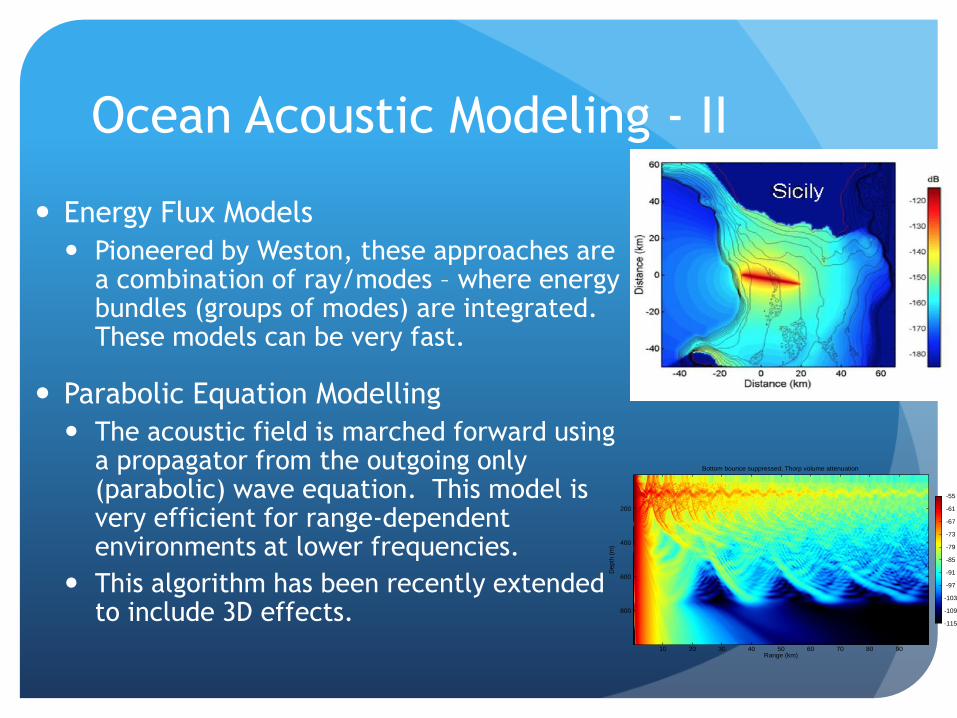
Ocean Acoustic Modeling - II

Energy Flux Models

Pioneered by Weston, these approaches are a combination of ray/modes – where energy bundles (groups of modes) are integrated. These models can be very fast.

Parabolic Equation Modelling

The acoustic field is marched forward using a propagator from the outgoing only (parabolic) wave equation. This model is very efficient for range-dependent environments at lower frequencies.

This algorithm has been recently extended to include 3D effects.

10 20 30 40 50 60 70 80 90

800

600

400

200

Bottom bounce suppressed, Thorp volume attenuation

Range (km)

De

pth

(m

)

-115

-109

-103

-97

-91

-85

-79

-73

-67

-61

-55

Ambient Noise Forecasting: Sources The local ambient noise is an incoherent combination of all sources in a

particular frequency band.

Temporal Variability

Minutes (passing ships)

Hours (sea-state)

Diurnal (biologics)

Weekly (weather, seismics)

Seasonal

Frequency Dependent Sources

Very Low frequency < 200 Hz

Ships, seismic surveys, baleen whales (Blue/Fin), Wind Farms, ice

Low Frequency (200-1 kHz)

Ships, Wind, Humpback Whales, Fish, ice cracking

Mid Frequency

Wind, Toothed Whales/Dolphins, Pile-Driving, Navy Sonars

High Frequency > 10 kHz

Snapping Shrimp, dolphins, ?

Ambient Noise Forecasting:

Propagation

Acoustic propagation conditions can effect the local

ambient noise

Sound speed profile – surface ducts can trap sound from

shallow sources

Wind can lead to rough surface, which reduces long-range

sound propagation

Soft/hard sediments can act as acoustic sponges/mirrors.

Interesting

Modelling/Measurement Examples

Seismic Airgun Modeling

CTBTO Crozet Study

Surface Shipping Noise (Data/Model)

CTBTO Acoustic Coverage Study

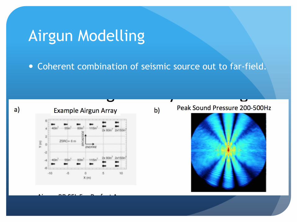
Airgun Modelling

Coherent combination of seismic source out to far-field.

HA04 Replacement Study

In view of the re-establishment of the Crozet Islands

hydrophone station (HA04), CTBTO initiated a number of

studies

Oceanographic and Acoustic Studies were performed to

investigate the optimal placement for survivability,

coverage and cost

For the acoustic study, the OASIS code (Peregrine-3D)

was used to investigate the impact of local bathymetric

and distant island/guyots/seamounts shielding on global

coverage

12

8 Hz Computation

2D vs. 3D Coverage for Crozet South

Relative 14% Increase in Coverage

8 Hz Computation

In order to evaluate candidate sites, a metric was chosen to be the % of

the earth covered as a function of Figure of Merit. (FOM = TL (with

positive Signal excess) = -(SL – AN)

For large sources

(earthquakes,

explosions) the 3D

predicted earth

coverage is

significantly

larger (~ 3%) than

the 2D

3D Diffraction Gain

from seamounts, ridges

3D refraction loss

from local

features

Shipping Dominated Environment

Data taken of Ft. Lauderdale USA

Shipping Noise Modelling Example

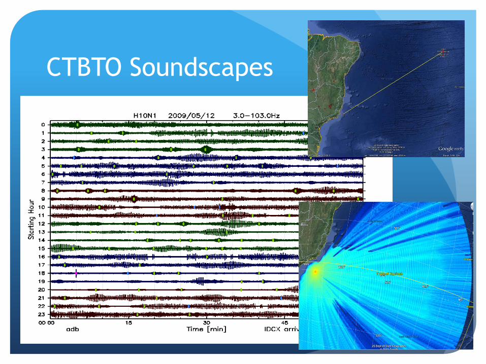
CTBTO Soundscapes

“Active Acoustic Space” Working w/ Jen Miksis-Olds @ ARL-PSU we are examining

the seasonal effects of an active acoustic space

This work addresses how far

mammals can detect other

mammals.

Future work will involve how far

in space can we extrapolate

noise measurements.

Measurements can help the

modelling

Modelling with historical databases for SVP, sediment can lead to very poor prediction capabilities.

The recent development of data-assimilative ocean models has with short time scales (~ 3 hour) and short spatial scales (~3 km) has greatly improved acoustic forecasting.

High resolution Bathymetry can be critical in shallow water environments

Direct (or inferred) measurements of the seafloor type are a requirement of accurate acoustic prediction.

A shipping source level database would be very useful.

POINT! – Make a Transmission Loss measurement part of the ambient noise measurement system.

Modelling can help the

measurements

Modelling can be done prior to the measurements of

ambient noise to determine best locations for limited

observations.

Modelling can be used after long-term ambient noise

measurements to extrapolate to different positions.

Conclusions / Knowledge Gaps

Propagation in underwater acoustics is critically dependent upon the local environment

Sound Speed

Bathymetry

Sediment Type

Area of the ocean – (r2) means errors in long-range attenuation leads to vast differences in area/volume illuminated

(16 log R?)

With a few simple measurements and current oceanographic modelling capabilities we can reliably estimate the ambient noise field. (Sources Level Calibrations)

FINAL POINT:

Propagation in the ocean is really complicated

Propagation in the ocean isn’t too hard to do reliably