Acoustic eigenanalysis of 2D open cavity with Vekua

approximations and the method of particular solutions

Alexandre Leblanc, Gilles Chardon

To cite this version:

Alexandre Leblanc, Gilles Chardon. Acoustic eigenanalysis of 2D open cavity with Vekuaapproximations and the method of particular solutions. Engineering Analysis with BoundaryElements, Elsevier, 2014, 43, pp.7. <10.1016/j.enganabound.2014.03.006>. <hal-01131092>

HAL Id: hal-01131092

https://hal.inria.fr/hal-01131092

Submitted on 17 May 2015

HAL is a multi-disciplinary open accessarchive for the deposit and dissemination of sci-entific research documents, whether they are pub-lished or not. The documents may come fromteaching and research institutions in France orabroad, or from public or private research centers.

L’archive ouverte pluridisciplinaire HAL, estdestinee au depot et a la diffusion de documentsscientifiques de niveau recherche, publies ou non,emanant des etablissements d’enseignement et derecherche francais ou etrangers, des laboratoirespublics ou prives.

Acoustic eigenanalysis of 2D open cavity with Vekua

approximations and the Method of Particular Solutions

Alexandre Leblanca,∗, Gilles Chardonb

aUniv Lille Nord de France, F-59000 Lille, France

UArtois, LGCgE, F-62400 Bethune, FrancebAustrian Academy of Sciences, Wohllebengasse 12-14, 1040 Wien, Austria

Abstract

This paper discusses the efficient extraction of acoustic resonances in 2Dopen cavities using a meshless method, the method of particular solutions.A first order, local non-reflecting boundary condition is chosen to account forthe opening and Fourier-Bessel functions are employed to approximate thepressure at the borders of the cavity and inside. A minimization problem isthen solved for the complex frequency range of interest. For the investigatedcavity, the minimum values obtained match those found in previous publishedstudies or by other numerical methods. But, unlike the perfectly matchedlayer absorbing boundary conditions now usually employed, this approach isfree from spurious eigenfrequencies. Moreover, the specific treatments of thegeometric singularities allow this method to be particularly efficient in thepresence of corner singularities.

Keywords: eigenanalysis, meshless method, Vekua theory

Introduction

Acoustic resonances of open cavities are crucial in many industrial, aero-nautical or marine applications. For transport, noise due to open cavitiesis omnipresent: open windows for cars [1], intercoach gaps for trains [2] orlanding gear traps for planes [3]. Acoustic characterization of urban environ-ments and streets is another field of active research, as the sound propagation

∗Corresponding authorEmail address: alexandre.leblanc@univ-artois.fr (Alexandre Leblanc)

Preprint submitted to Elsevier March 14, 2014

is often treated through an open waveguide [4]. Beyond noise considerations,musical acoustics is also concerned in studying these resonances, especiallyfor the design of wind or string instruments. The last decades have broughta deep understanding of the mechanisms behind the noise produced by theinteraction of an air flow with an open cavity [3, 5], but the suppression, orat least the significant reduction of the feedback loop of this coupling is stillchallenging [5]. Active control techniques are the most promising answers [6],but a critical issue for those tools is the location of the secondary sourcesand error sensor [7]. Indeed, nodal lines must be avoided in order to have anefficient noise control on each acoustic mode of interest. Moreover, knowingthe frequencies of these resonances at the design phase is also necessary ifimplementing effective passive control techniques. Often, the task can be re-duced to the determination of acoustic resonances of the open cavity withoutflow. Indeed, the acoustic cavity tones generated are practically independentof the velocity flow at low Mach numbers.

Eigenanalysis of cavities can be treated in numerous ways. In the casesof simple geometries, analytic solutions are likely to be obtained at low com-putational cost and high precision (according to the possible simplificationsmade on the real geometry). The effective resonances can be also obtainedthrough an experimental setup, which is prone to give by definition rele-vant answers, but often comes with prohibitive cost and with only minimumquantitative information. So, a good addition (nowadays, it even tends tobe a replacement) is to build and solve numerical models, sufficiently repre-sentative of the physics involved here. These models are based on numericaltechniques such as, and for the most part, the finite element method (FEM).However, it can be computationally intensive at high frequencies or in thepresence of singularities (e.g. corner singularities). Alternative methodshave emerged to lower this shortcoming, one can cite the boundary elementmethod (BEM) and meshless methods as the method of fundamental so-lutions (MFS). Unfortunately, these methods come with other difficulties,leaving, decades after decades, the FEM as the routine tool for most ofacoustic studies. So, it is no surprise that the majority of attempts for per-forming the numerical eigenanalysis of open cavities is based on a similarapproach to that of Koch [8], who solved the Helmholtz wave equation byFEM, and using a perfectly matched layer (PML). The main idea is to coverthe original open cavity by another fluid domain, bounded by a baffle in theextension of the opening and otherwise, by a non-reflecting boundary (fea-ture brought by the PML). While robust, this approach exhibits the major

2

drawback of introducing spurious modes in the solution spectrum, in addi-tion to be sometimes high-demanding from a computational point of view.Indeed, automatic distinction between artificial (PML domain) and relevanteigenvalues (cavity) remains challenging. Before the advent of PML, two ap-proaches have been widely developed in order to avoid nonphysical reflectionsat artificial boundaries (those that allow the truncation of physical domain).The first set of these non-reflecting boundary conditions (NRBC) brings lo-cal relation between the pressure and its derivative, while the other family isan exact NRBC known as Dirichlet-to-Neumann (DtN) map [9]. The meritsand drawbacks of these different approaches have been thoroughly discussedby Givoli [10] and Tsynkov [11]. These authors state that none is clearly su-perior to others, and that the choice should be based on arbitrary constraints(robustness, ease of implementation or computational efficiency).

In this paper, eigenanalysis of 2D open cavities by the method of par-ticular solutions (MPS) with local NRBC is discussed. The MPS is dedi-cated to the eigenanalysis of elliptic operators and was originally proposedby Fox, Henrici and Moller [12]. It has generated as much enthusiasm (forits simplicity) as disappointment: while efficient for simple geometries, sta-bility problems arise for more complicated domains. Recently, Betcke andTrefethen [13] proved that these failures are due to a single cause: the orig-inal MPS does not impose nonzero eigenfunctions. With the introductionof interior collocation points, Betcke and Trefethen circumvent this issue,substituting the determinant computation in [12] by the resolution of a gen-eralized eigenvalue problem. Now a robust method, the MPS offers someadvantages in the present context: the formulation is straightforward, con-sistent with local ABC, and multiple eigenvalues are easy to determine, withthe associated eigenspaces readily recovered.

This algorithm needs an approximation scheme for the solutions to theconsidered partial differential equation. In [12, 13], fractional Fourier-Besselfunctions were used, while Fourier-Bessel and modified Fourier-Bessel wereemployed in [14] to treat the case of Kirchhoff-Helmholtz plates. The approx-imation given by the MFS could also be used (note here that the MPS is acomputational method, i.e. an algorithm, while the MFS is an approximation

method). However the approximation schemes usually used in conjonctionwith the MPS are free from any spurious modes [13], unlike the MFS [15].

In order to take into account the cavity opening, local NRBC are con-sidered here, linking only nearby neighbors of a boundary point. For thewave equation, Bayliss et al. [16] constructed a sequence of ABC based on

3

the asymptotic expansion of the solution to the exterior Helmholtz equation.Since the condition is written in polar coordinates, it is most convenient whenthe virtual boundary is a circle. Li and Cendes [17] proposed a similar NRBCusing the full convergent expansion of the solution (see Medvinsky [18] for thelink between both formulations). While the Bayliss NRBC is best known, theLi–Cendes form is expected to be more efficient if the non-reflecting boundaryis close to the scatterer, which is the case in the present context.

The layout of the paper is as follows. Section 1 presents the computationalmodel leading to the approximation of open cavity eigenmodes. To this end,local non-reflecting boundary conditions, the method of particular solutionand the Vekua theory are briefly recalled. Numerical results are presented insection 2 and are also compared with solutions obtained by the FEM withPML [8]. Finally, the main conclusions are outlined in section 3.

1. Eigenmodes of an open cavity

An acoustic open cavity filled with fluid in a semi-infinite wall is con-sidered, as sketched in Fig. 1. The problem of interest consists of the iden-

Figure 1: Rectangular open cavity

r

dL/2 L/2

x

yΩ

Γt

Ωt

tification of the eigenmodes of this cavity. This problem is defined in theunbounded domain Ω by the Helmholtz equation and its boundary condi-

4

tions as

∆u+ k2u = 0 in Ω (1)

∂u

∂n= 0 on Γ (2)

limr→∞

r1/2 (ur − iku) = 0 uniformly in θ (3)

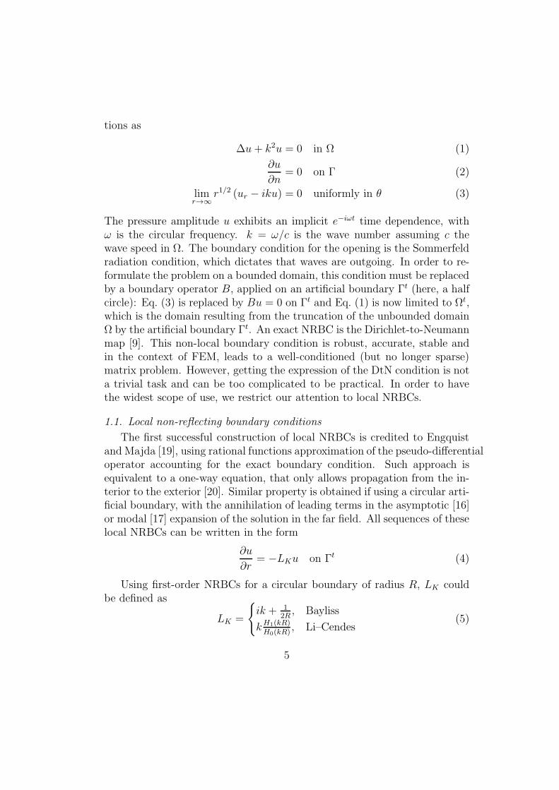
The pressure amplitude u exhibits an implicit e−iωt time dependence, withω is the circular frequency. k = ω/c is the wave number assuming c thewave speed in Ω. The boundary condition for the opening is the Sommerfeldradiation condition, which dictates that waves are outgoing. In order to re-formulate the problem on a bounded domain, this condition must be replacedby a boundary operator B, applied on an artificial boundary Γt (here, a halfcircle): Eq. (3) is replaced by Bu = 0 on Γt and Eq. (1) is now limited to Ωt,which is the domain resulting from the truncation of the unbounded domainΩ by the artificial boundary Γt. An exact NRBC is the Dirichlet-to-Neumannmap [9]. This non-local boundary condition is robust, accurate, stable andin the context of FEM, leads to a well-conditioned (but no longer sparse)matrix problem. However, getting the expression of the DtN condition is nota trivial task and can be too complicated to be practical. In order to havethe widest scope of use, we restrict our attention to local NRBCs.

1.1. Local non-reflecting boundary conditions

The first successful construction of local NRBCs is credited to Engquistand Majda [19], using rational functions approximation of the pseudo-differentialoperator accounting for the exact boundary condition. Such approach isequivalent to a one-way equation, that only allows propagation from the in-terior to the exterior [20]. Similar property is obtained if using a circular arti-ficial boundary, with the annihilation of leading terms in the asymptotic [16]or modal [17] expansion of the solution in the far field. All sequences of theselocal NRBCs can be written in the form

∂u

∂r= −LKu on Γt (4)

Using first-order NRBCs for a circular boundary of radius R, LK couldbe defined as

LK =

ik + 12R, Bayliss

kH1(kR)H0(kR)

, Li–Cendes(5)

5

where Hn (kR) are Hankel functions. The Li–Cendes expansion is used inthis paper, since only the low-frequency spectrum (where the asymptotic ex-pansion of Bayliss is expected to be less efficient [21]) is of particular concernhere.

1.2. The method of particular solutions

The basic idea behind the MPS is to consider separately the spaces ofsolutions of the Helmholtz equation for different wave numbers. In eachsolution spaces, a nonzero function satisfying the boundary conditions is thenan eigenmode. As originally formulated for Dirichlet boundary conditions,the MPS needs N points xj on the border of the domain, associated with Nfunctions φi spanning a subspace which approximates the set of solutions tothe Helmholtz equation with a given wavenumber k. In order to obtain theeigenfrequencies, a square matrix M (k) containing the values of φ at the Npoints is build and its determinant computed:

det (M (k)) =

∣

∣

∣

∣

∣

∣

∣

φ1 (x1) · · · φN (x1)...

...φ1 (xN ) · · · φN (xN )

∣

∣

∣

∣

∣

∣

∣

(6)

If a linear combination of functions is zero on the border, then the determi-nant is zero. As only a finite dimensional-space is considered, the boundarycondition is unlikely to be exactly satisfied, and the eigenfrequencies are ob-tained as the local minima of this determinant. As pointed out by Betcke andTrefethen [13], this simple method has limitations. First, the discretizationof the solutions space and boundaries sampling must be of equal size. Sec-ond, M(k) gets ill-conditioned as the number of functions grows. To avoidthese problems, the same authors suggest to solve the following optimizationproblem:

τ (k) = minu

‖Tu‖2L2(∂Ω) (7)

under the constraints that ‖u‖2L2(∂Ω) = 1 and that u is solution to theHelmholtz equation, and where T is the trace operator on the boundary∂Ω. If the tension τ (k) is zero, then there is a nonzero function in Ω that iszero on its boundary, and k is an eigenfrequency. For a family of functions(φi) chosen for the approximation of the solutions of the Helmholtz equationwith wavenumber k, and with expansion coefficients u = (u1, . . . , uN), we

6

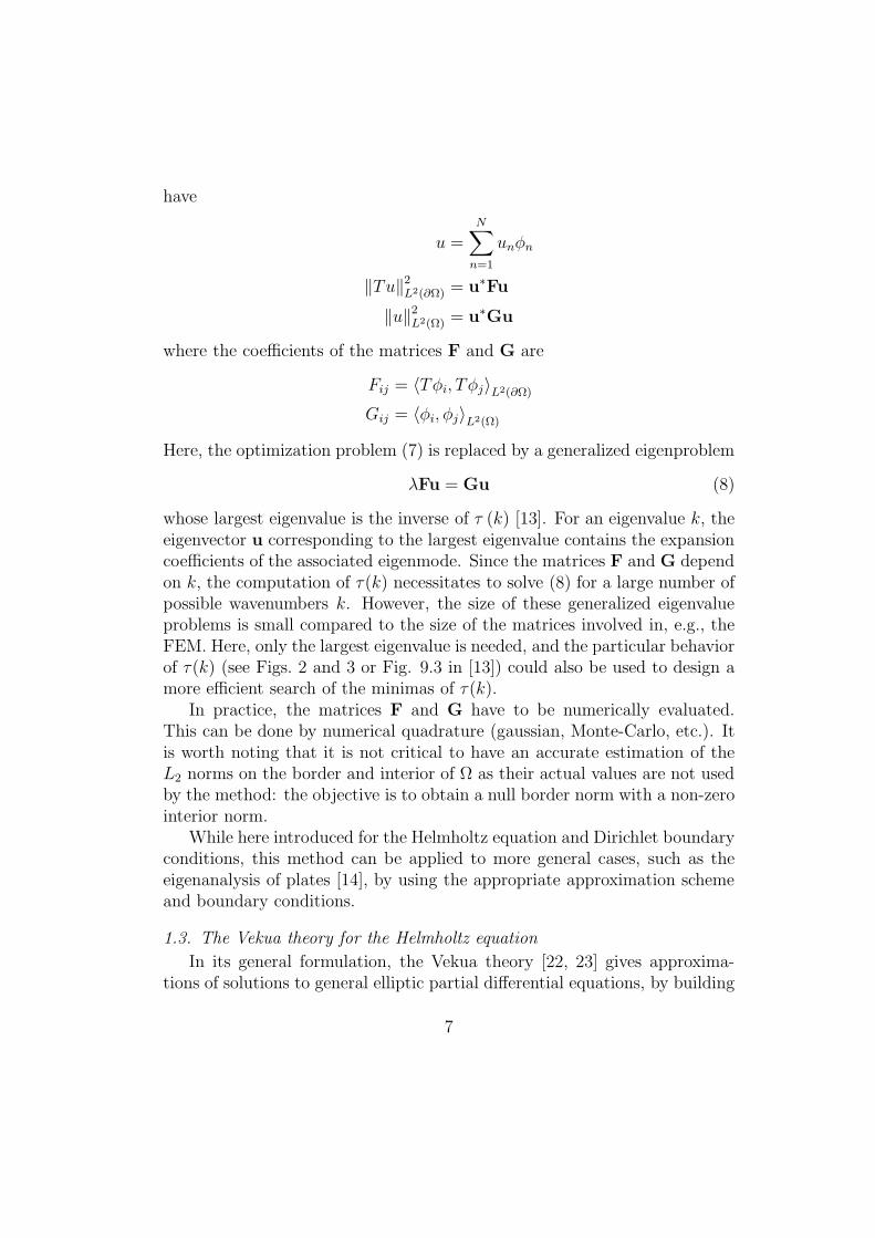
have

u =N∑

n=1

unφn

‖Tu‖2L2(∂Ω) = u∗Fu

‖u‖2L2(Ω) = u∗Gu

where the coefficients of the matrices F and G are

Fij = 〈Tφi, Tφj〉L2(∂Ω)

Gij = 〈φi, φj〉L2(Ω)

Here, the optimization problem (7) is replaced by a generalized eigenproblem

λFu = Gu (8)

whose largest eigenvalue is the inverse of τ (k) [13]. For an eigenvalue k, theeigenvector u corresponding to the largest eigenvalue contains the expansioncoefficients of the associated eigenmode. Since the matrices F and G dependon k, the computation of τ(k) necessitates to solve (8) for a large number ofpossible wavenumbers k. However, the size of these generalized eigenvalueproblems is small compared to the size of the matrices involved in, e.g., theFEM. Here, only the largest eigenvalue is needed, and the particular behaviorof τ(k) (see Figs. 2 and 3 or Fig. 9.3 in [13]) could also be used to design amore efficient search of the minimas of τ(k).

In practice, the matrices F and G have to be numerically evaluated.This can be done by numerical quadrature (gaussian, Monte-Carlo, etc.). Itis worth noting that it is not critical to have an accurate estimation of theL2 norms on the border and interior of Ω as their actual values are not usedby the method: the objective is to obtain a null border norm with a non-zerointerior norm.

While here introduced for the Helmholtz equation and Dirichlet boundaryconditions, this method can be applied to more general cases, such as theeigenanalysis of plates [14], by using the appropriate approximation schemeand boundary conditions.

1.3. The Vekua theory for the Helmholtz equation

In its general formulation, the Vekua theory [22, 23] gives approxima-tions of solutions to general elliptic partial differential equations, by building

7

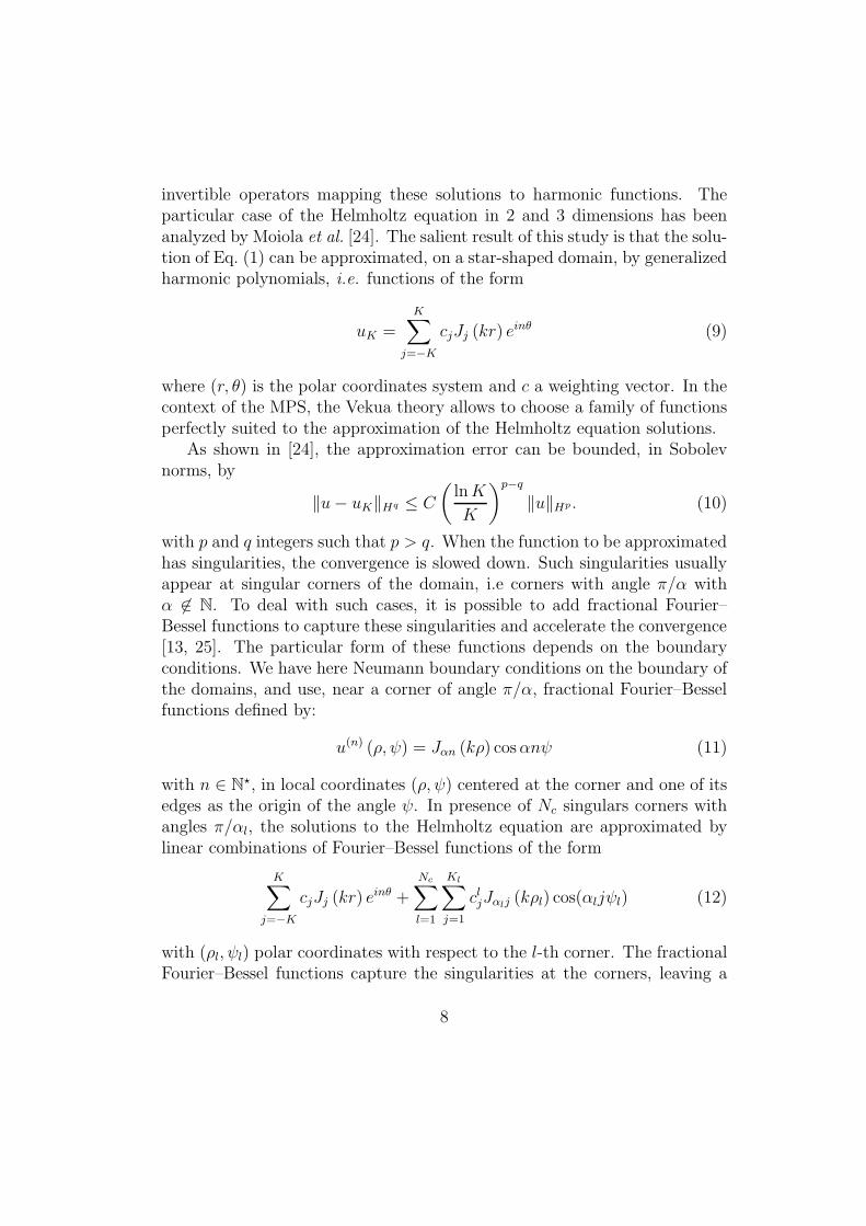
invertible operators mapping these solutions to harmonic functions. Theparticular case of the Helmholtz equation in 2 and 3 dimensions has beenanalyzed by Moiola et al. [24]. The salient result of this study is that the solu-tion of Eq. (1) can be approximated, on a star-shaped domain, by generalizedharmonic polynomials, i.e. functions of the form

uK =K∑

j=−K

cjJj (kr) einθ (9)

where (r, θ) is the polar coordinates system and c a weighting vector. In thecontext of the MPS, the Vekua theory allows to choose a family of functionsperfectly suited to the approximation of the Helmholtz equation solutions.

As shown in [24], the approximation error can be bounded, in Sobolevnorms, by

‖u− uK‖Hq ≤ C

(

lnK

K

)p−q

‖u‖Hp. (10)

with p and q integers such that p > q. When the function to be approximatedhas singularities, the convergence is slowed down. Such singularities usuallyappear at singular corners of the domain, i.e corners with angle π/α withα 6∈ N. To deal with such cases, it is possible to add fractional Fourier–Bessel functions to capture these singularities and accelerate the convergence[13, 25]. The particular form of these functions depends on the boundaryconditions. We have here Neumann boundary conditions on the boundary ofthe domains, and use, near a corner of angle π/α, fractional Fourier–Besselfunctions defined by:

u(n) (ρ, ψ) = Jαn (kρ) cosαnψ (11)

with n ∈ N⋆, in local coordinates (ρ, ψ) centered at the corner and one of its

edges as the origin of the angle ψ. In presence of Nc singulars corners withangles π/αl, the solutions to the Helmholtz equation are approximated bylinear combinations of Fourier–Bessel functions of the form

K∑

j=−K

cjJj (kr) einθ +

Nc∑

l=1

Kl∑

j=1

cljJαlj (kρl) cos(αljψl) (12)

with (ρl, ψl) polar coordinates with respect to the l-th corner. The fractionalFourier–Bessel functions capture the singularities at the corners, leaving a

8

residual that is more regular than the original function, allowing a fasterconvergence of the approximation by regular Fourier–Bessel functions, asindicated by (10).

1.4. Approximation of open cavity eigenmodes

The results and techniques discussed above are now pieced together toyield a numerical method to compute eigenmodes of open cavities.

We approximate the solutions to the Helmholtz equation on the domainΩt, assumed to be star-shaped, with Fourier–Bessel function. As the domainis likely to have singular corners, e.g. at the junction of the cavity with thebaffle, we add fractional Fourier–Bessel functions to the family of functions.The boundary conditions are Neumann boundary conditions on Γ and thelocal NRBC given by Eq. (5). The corresponding tension is then

t =

∫

Γ

∣

∣

∣

∣

∂u

∂n

∣

∣

∣

∣

2

+

∫

Γt

∣

∣

∣

∣

∂u

∂n+ LKu

∣

∣

∣

∣

2

(13)

where u is here approximated by the Fourier–Bessel functions of the previoussection. For each frequency, the goal is to compute the set of cn leading tolowest value of t. The complex eigenfrequencies are the local minimas of thetension. It is worth noting that the condition number of the matrix definingthe tension is stable when evaluated at the sought eigenvalues.

2. Numerical results

In the following investigations, the Fourier-Bessel functions are centeredat the origin, which is also the center of the circular NRBC. While the domainis not necessarily star-shaped with respect to a disk around this center, andthe results by Moiola et al. not directly applicable, it is shown in the appendixthat the choice of the center has no incidence on the approximation rate. Forthe treatment of the singularities which can arise at corners of the studieddomains, fractional Fourier-Bessel are used, centered on these corners [13, 25].

The first investigation deals with the square open cavity. This case isthe same that the one depicted in Fig. 2b of Koch’s paper [8]. Figure 2compares the results obtained with the present MPS formulation, using K =32 Fourier–Bessel functions and 40 expansions terms for the opening corners(cf. Eq. 11), with those of Koch (FEM with PML). Here, Lk is the first-order Li–Cendes NRBC with R = L/2. The cavity is discretized with 58

9

equally spaced boundary nodes and 100 nodes on the NRBS boundary toestimate the coefficients of the matrix F, and 100 nodes inside the cavity forG. Overall, the eigenmodes found with the present approach coincide well

Figure 2: Open square cavity resonances: color field is (1/t) on a decibel scale (dB) usingLi–Cendes NRBC (with R = L/2), the ’o’ marks are the values obtained by Koch [8] [Fig.2b]

Re(K/2π)

Im(K

/2π

)

0 0.5 1 1.5 2 2.5 3−0.12

−0.1

−0.08

−0.06

−0.04

−0.02

dB0

10

20

30

with those found in [8]. The two first values very close to the imaginary axisare missing with the MPS as they are due to the discrete approximation ofthe continuous spectrum by the PML boundaries. Also, it is worth notingthat the additional PML modes polluting the solution are not shown here,as in [4, 8]. These eigenvalues, only linked to the PML parameters, arefiltered out thanks to their corresponding eigenmodes but at the cost ofa post-processing analysis, which can be time consuming. Such procedureis completely avoided using the MPS approach. For the weakly dampedeigenvalues (the physically dominant modes), the difference between the twocalculations are low. The discrepancies for the higher damped modes are duefor the most part to the location of the NRBC, being in the near-field. Thesedifferences may also be linked to the treatment of the cavity opening corners(eg. the number of expansion terms used) when Γ does not include the semi-infinite wall. Figure 3 compares the results between three approaches foran identical domain Ωf (R = 2L). The 58 additional nodes discretizing thewall further enhance the MPS efficiency. Indeed, and in addition to betterresults for the most damped modes, a better contrast is obtained, whichmay be crucial to identify close spaced eigenfrequencies. Raw results for aFEM simulation (12366 triangular elements) with Li–Cendes NRBC are alsoshown in Fig. 3. The MPS clearly benefits of the specific treatment of theopening corners. Perhaps more importantly, the MPS proves to be free fromspurious eigenvalues, those linked to the half-disk above the open cavity, as

10

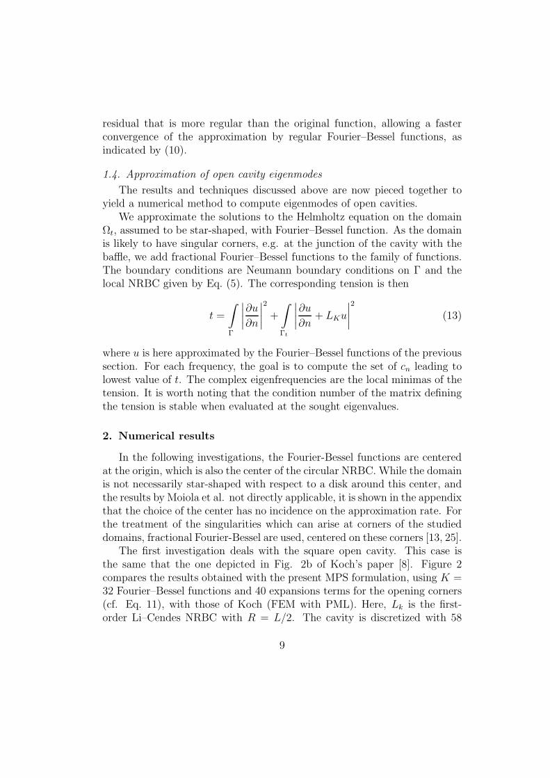
small eigenfunctions on boundary points automatically enforce unit normsat interior points [13]. These examples demonstrate the ability of the MPS

Figure 3: Open square cavity resonances using Li–Cendes NRBC (with R = 2L): colorfield is the MPS results, dots are the values obtained with a FEM solver. The ’o’ marksare the values obtained by Koch [8] [Fig 2b]

Re(K/2π)

Im(K

/2π

)

0 0.5 1 1.5 2 2.5 3−0.12

−0.1

−0.08

−0.06

−0.04

−0.02

dB0

10

20

30

40

50

to efficiently perform the eigenanalysis of open cavities.We now investigate implementation issues, such as the influence of the

ratio R/L, the choice of the sampling points and the approximation order onthe accuracy.

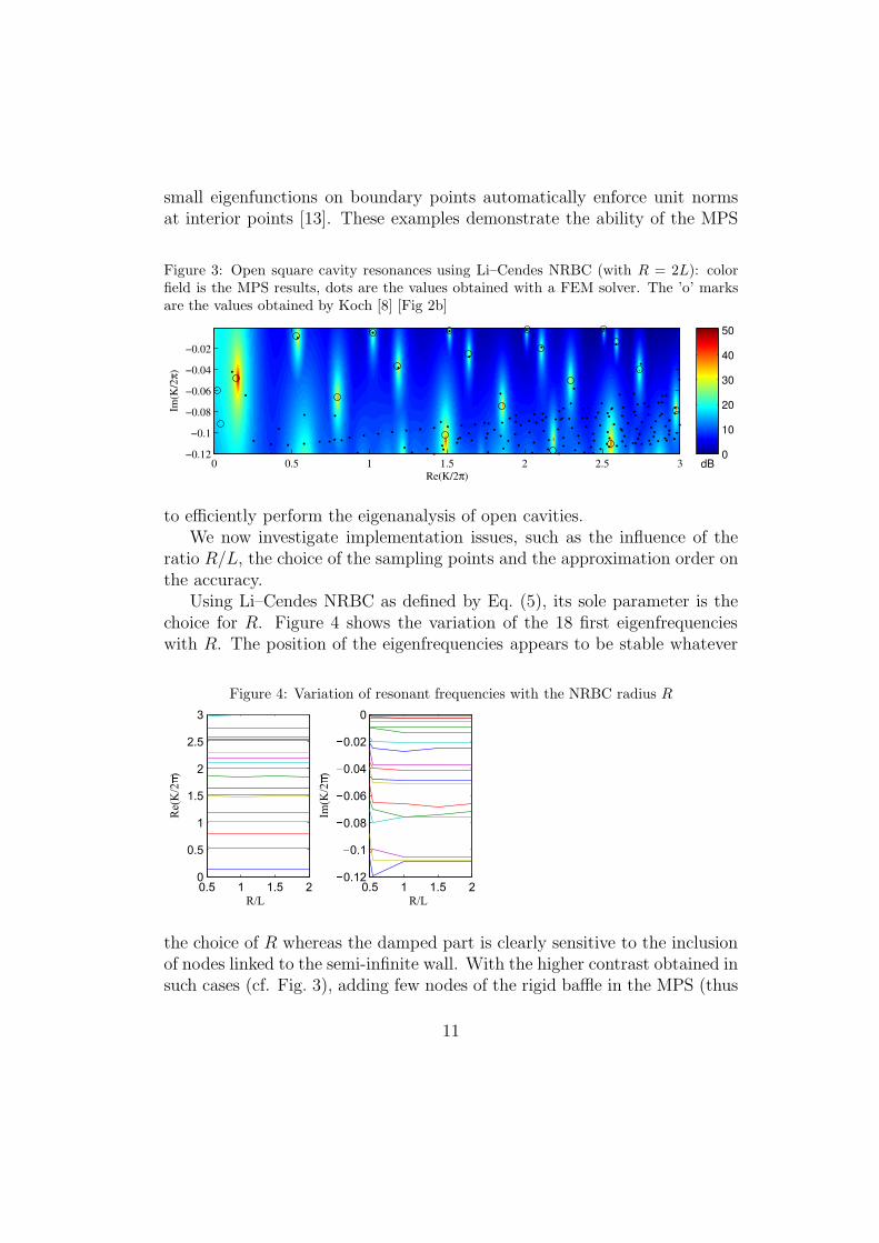
Using Li–Cendes NRBC as defined by Eq. (5), its sole parameter is thechoice for R. Figure 4 shows the variation of the 18 first eigenfrequencieswith R. The position of the eigenfrequencies appears to be stable whatever

Figure 4: Variation of resonant frequencies with the NRBC radius R

0.5 1 1.5 20

0.5

1

1.5

2

2.5

3

R/L

Re(K/2)

0.5 1 1.5 20.12

0.1

0.08

0.06

0.04

0.02

0

R/L

Im(K/2)

the choice of R whereas the damped part is clearly sensitive to the inclusionof nodes linked to the semi-infinite wall. With the higher contrast obtained insuch cases (cf. Fig. 3), adding few nodes of the rigid baffle in the MPS (thus

11

leading to a somehow far-field NRBC) seems to be a necessity, especiallyconsidering the low numerical cost induced.

For the interior points, it seems at first legitimate to question the impor-tance of their number and their position on the results. The answer whichencompasses these two preoccupations is given by Betcke and Trefethen:

A random distribution of interior points has always proved ef-fective. In principle the method would fail if all points fell inregions where the eigenfunction is close to zero, but this is easilyprevented by taking a healthy number of randomly distributedpoints. For the speed of the algorithm there is not much differ-ence between 50 or 500 interior points

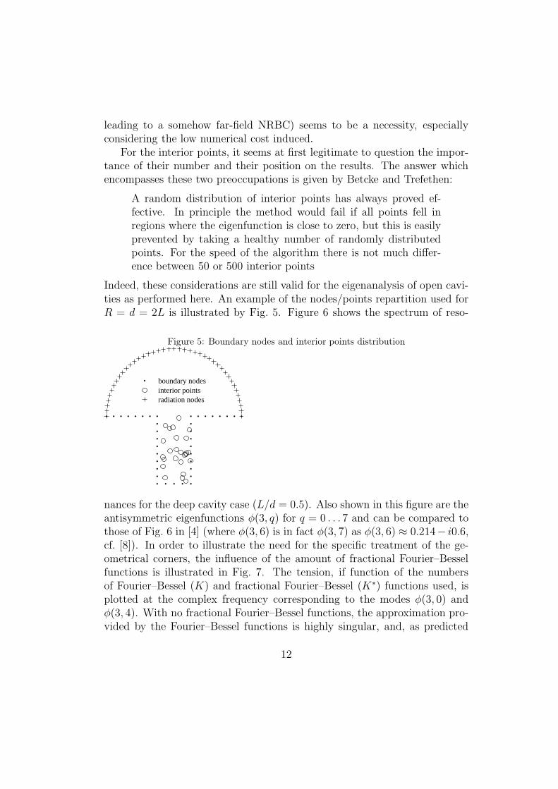
Indeed, these considerations are still valid for the eigenanalysis of open cavi-ties as performed here. An example of the nodes/points repartition used forR = d = 2L is illustrated by Fig. 5. Figure 6 shows the spectrum of reso-

Figure 5: Boundary nodes and interior points distribution

boundary nodesinterior pointsradiation nodes

nances for the deep cavity case (L/d = 0.5). Also shown in this figure are theantisymmetric eigenfunctions φ(3, q) for q = 0 . . . 7 and can be compared tothose of Fig. 6 in [4] (where φ(3, 6) is in fact φ(3, 7) as φ(3, 6) ≈ 0.214− i0.6,cf. [8]). In order to illustrate the need for the specific treatment of the ge-ometrical corners, the influence of the amount of fractional Fourier–Besselfunctions is illustrated in Fig. 7. The tension, if function of the numbersof Fourier–Bessel (K) and fractional Fourier–Bessel (K∗) functions used, isplotted at the complex frequency corresponding to the modes φ(3, 0) andφ(3, 4). With no fractional Fourier–Bessel functions, the approximation pro-vided by the Fourier–Bessel functions is highly singular, and, as predicted

12

Figure 6: Samples eigenfunction obtained with MPS for a deep open cavity (d = 2L, see[4])

Re(K/2π)

Im(K

/2π

)

1.5 1.6 1.7 1.8 1.9 2 2.1 2.2 2.3 2.4

−0.08

−0.06

−0.04

−0.02

0

| φ(3,0) | | φ(3,1) | | φ(3,2) | | φ(3,3) | | φ(3,4) | | φ(3,5) | | φ(3,6) | | φ(3,7) |

by Eq. (10), the convergence is very slow. Adding fractional Fourier–Besselfunctions to the family used to approximate the Helmholtz solutions allowsa much faster convergence, but as the estimated complex frequency is notexactly the true frequency, the tension still converges to a low, but nonzero,value. Being more general than the method depicted in [4], the present ap-

Figure 7: Influence of the number of fractional Fourier–Bessel functions used (K∗) for thedetermination of the antisymmetric modes φ(3, 0) and φ(3, 4) (cf. Fig. 6)

10 20 30 40 50 60

−10

−8

−6

−4

−2

0

log(|t K

,K∗|)

K

φ(3,0)

10 20 30 40 50 60

−12

−10

−8

−6

−4

−2

0

K

φ(3,4)

: K∗ = 0: K∗ = 5: K∗ = 10: K∗ = 15: K∗ = 20

proach also leads to accurate determination of the eigenmodes when appliedto arbitrary shaped open cavities (cf. Fig. 8). For this cavity, the four ge-

13

ometric singularities are handled with 32 Fourier–Bessel functions and theboundary is discretized with 72 nodes. The eigenfrequency and correspond-ing pressure pattern computed by the MPS and shown in Fig. 8 are closeto those calculated with a commercial FEM solver (both methods using aLi–Cendes NRBC with R = 2L). For this last numerical experiment, con-verged eigenvalues are obtained using more than 5000 quadratic triangularelements, where the MPS solve a generalized eigenproblem of size 125.

Figure 8: Eigenfunction (absolute pressure) comparison between MPS and FEM, thecavity is open at its largest side

(a) MPS, K/2π = 2.33−i0.46 (b) FEM, K/2π = 2.34−i0.49

3. Conclusion

The method of particular solutions has been employed with a local non-reflecting boundary condition for the eigenmodes of open cavities. Followingthe Vekua theory for the Helmholtz equation, generalized harmonic polyno-mials are used to approximate the unknown pressure. The functions param-eters are determined thanks to an optimization problem. In the case of asquare cavity, this approach gives eigenvalues similar to those found by aFEM eigenanalysis. Fourier–Bessel functions of fractional orders at geomet-ric singularities bring satisfying results even if the discretization is limited tothe cavity. However, inserting few nodes of the exterior boundary (eg. therigid baffle) improves both the accuracy and interpretation of results (highercontrast for the minimization problem, which may be essential in the case ofclosely spaced frequencies). A remarkable feature of this approach is that nospurious modes are produced, thanks to randomly located points inside thecavity. This gives this approach a real interest for numerical computations.For example, it can be used for the urban noise propagation, as performedin [4], with a more realistic street canyon geometry and without having toperform a tedious sorting between spurious and effective eigenmodes.

14

Appendix A. Approximation by decentered Fourier-Bessel func-

tions

In [24], the Fourier-Bessel approximation for the solutions to the Helmholtzequation is proved when the domain Ω, on which the solutions are consid-ered, is star-shaped with respect to a disk D of radius δ around the origin ofthe polar coordinates. Thus, in Sobolev norms:

‖u− uN‖Hq(Ω) ≤ C

(

logN

N

)p−q

‖u‖Hp(Ω), (A.1)

where

uN =N∑

n=−N

αNn Jn(kr)einθ. (A.2)

We prove here that the rate of convergence is retained when the center ofthe polar coordinates is moved. Results on Bessel functions are availablein [26, 27].

Using Graf’s theorem, the origin of the Fourier-Bessel functions can bemoved:

uN =

N∑

n=−N

αNn∑

m∈Z

Jm+n(kR)ei(n+m)Θ

×Jm(kρ)eimψ(A.3)

where (ρ, ψ) are the polar coordinates with respect to the new center, ofpolar coordinates (R,Θ). Then, u can be approximated by:

uN =

N∑

n=−N

αNn

3N+2∑

m=−3N−2

Jm+n(kR)ei(m+n)Θ

×Jm(kρ)eimψ.(A.4)

For orders larger than kρm, the Fourier-Bessel functions are increasing on(0, ρm) (cf. [27] Eq. (A.4)), where ρm is the maximal distance between apoint of Ω and the center of the polar coordinates. Thus, for N > kρm, the

15

approximation error is:

|uN − uN | =

∣

∣

∣

∣

∣

∣

N∑

n=−N

αNn∑

|m|>3N+2

Jm+n(kR)

×ei(n+m)ΘJm(kρ)eimψ

∣

∣ (A.5)

≤N∑

n=−N

|αNn |∑

|m|>3N+2

|Jm+n(kR)|

× |Jm(kρm)| (A.6)

On the disk D, we have:

∫

D

|αNn Jn(kr)|2 ≤∫

D

|uN |2 (A.7)

≤ ‖uN‖2L2(Ω) (A.8)

as the Fourier–Bessel functions are orthogonal on the disk D. As ‖uN‖L2(Ω)

converges to ‖u‖L2(Ω), for high orders N we have ‖uN‖L2(Ω) ≤ C‖u‖L2(Ω)

where C is a constant larger that 1. Using

∫

D

|Jn(kr)|2 = 2

∞∑

l=0

(n+ 1 + 2l)J2n+1+2l(kδ) (A.9)

≥ J2n+1(kδ), (A.10)

gives a bound on αNn :

|αNn | ≤C‖u‖L2(Ω)

Jn+1(kδ)(A.11)

In the case where Jn+1(kδ) is zero for some n, a smaller δ′ such that Jn+1(kδ′) 6=

0 for all n can be used. Note that in a given interval (0, x), the Bessel func-tions have only a finite number of zeros as the Bessel functions Jn with n > xare strictly positive (cf. [27] Eq. (A.4)) for x > 0. It is therefore always pos-sible to find such a radius δ′.

16

The error between uN and uN can be bounded by:

|uN − uN | ≤ CN∑

n=−N

‖u‖L2(Ω)

|Jn+1(kδ)|

×∑

|m|>3N+2

|Jm+n(kR)||Jm(kρm)| (A.12)

≤ (2N + 1)C‖u‖L2(Ω)

|J2N+2(kR)||JN+1(kδ)|

×∑

|m|>3N+2

|Jm(kρm)|. (A.13)

Indeed, we have infn≤N |Jn+1(kδ)| = min(infn≤kδ |Jn+1(kδ)|, infkδ<n≤N |Jn+1(kδ)|).For n > kδ, |Jn+1(kδ)| as a function of n is decreasing (cf. [27] Eq. (A.6)), andwe have infn≤N |Jn+1(kδ)| = min(infn≤kδ |Jn+1(kδ)|, |JN+1(kδ)|). |Jn+1(kδ)|tends to 0, and we have, for sufficiently high ordersN , |JN+1(kδ)| ≤ infn≤kδ |Jn+1(kδ)|and infn≤N |Jn+1(kδ)| = |JN+1(kδ)|. Likewise, as |m+ n| ≥ 2N + 2, we have|Jm+n(kR)| ≤ |J2N+2(kR)|.

The Bessel functions have the following asymptotic approximation forlarge orders:

Jn(x) ∼1√2πn

(ex

2n

)n

.

The series in (A.13) being convergent, the error can be bounded by

|uN − uN | ≤ C ′N

(

(ekR)2

2ekδ

1

8(N + 1)

)N+1

‖u‖L2(Ω) (A.14)

where C ′ is a positive constant. The error decreases faster than exponentiallyand, in particular, faster than the error between u and uN . Similar resultscan be obtained for the derivatives of uN , as taking the derivatives will onlychange the terms appearing in the series in (A.13). Finally, (A.1) is recovered:

‖u− uN‖Hq(Ω) ≤ C

(

logN

N

)p−q

‖u‖Hp(Ω), (A.15)

where uN involves Fourier-Bessel functions of orders up to 4N + 2. Whilethe domain has to be star-convex with respect to a disk, the center of theFourier-Bessel can be chosen outside of this disk, even outside of the domainof interest. The onset of the asymptotical regime is however likely to beslower than in the original approximation (cf. Eq. (10)), depending on thewavenumber k, the distance between the two centers R and the radius of D.

17

Acknowledgement

Gilles Chardon is supported by the Austrian Science Fund (FWF) START-project FLAME (Frames and Linear Operators for Acoustical Modeling andParameter Estimation; Y 551-N13).

[1] Ota DK, Becker T, Sturzenegger T, Chakravarthy SR. Computationalstudy of resonance suppression of open sunroofs. J Fluid Eng-T ASME1994;116(4):877–882.

[2] Mellet C, Letourneaux F, Poisson F, Talotte C. High speed train noiseemission: Latest investigation of the aerodynamic/rolling noise contri-bution. J Sound Vib 2006;293(3-5):535–546.

[3] Rowley CW, Williams DR. Dynamics and control of high-Reynolds-number flow over open cavities. Annu Rev Fluid Mech 2006;38(1):251–276.

[4] Pelat A, Felix S, Pagneux V. On the use of leaky modes in open waveg-uides for the sound propagation modeling in street canyons. J AcoustSoc Am 2009;126(6):2864–2872.

[5] Gloerfelt X. Cavity noise. In: VKI Lectures, Aerodynamic noise fromwall-bounded flows. Von Karman Institute 2009.

[6] Illingworth SJ, Morgans AS, Rowley CW. Feedback control offlow resonances using balanced reduced-order models. J Sound Vib2011;330(8):1567–1581.

[7] Ortiz S., Plenier CL, Cobo P. Efficient modeling and experimental vali-dation of acoustic resonances in three-dimensional rectangular open cav-ities. Appl Acoust 2013;74(7):949–957.

[8] Koch W. Acoustic resonances in rectangular open cavities. AIAA Jour-nal 2005;43(11):2342–2349.

[9] Keller JB, Givoli D. Exact non-reflecting boundary conditions. J Com-put Phys 1989;82(1):172–192.

[10] Givoli D. Recent advances in the DtN FE Method. Arch Comput Meth-ods Engrg 1999;6(2):71–116.

18

[11] Tsynkov SV. Numerical solution of problems on unbounded Domains.A Review. Appl Numer Math 1998;27(4):465–532.

[12] Fox L, Henrici P, Moler C. Approximations and bounds for eigenvaluesof elliptic operators. SIAM J Numer Anal 1967;4(1):89–102.

[13] Betcke T, Trefethen LN. Reviving the method of particular solutions.SIAM Rev 2005;47(3):469–491.

[14] Chardon G, Daudet L. Low-complexity computation of plate eigenmodeswith Vekua approximations and the method of particular solutions.Comput Mech 2013;52(5):982–992.

[15] Tsai C.C., Young D.L., Chen C.W., Fan C.M. The method of funda-mental solutions for eigenproblems in domains with and without interiorholes. P Roy Soc Lond A Mat 2006;462 (2069):1443–1466.

[16] Bayliss A, Gunzburger M, Turkel E. Boundary conditions for the nu-merical solution of elliptic equations in exterior regions, SIAM J ApplMath 1982;42(2):430–451.

[17] Li Y, Cendes ZJ. Modal expansion absorbing boundary conditionsfor two-dimensional electromagnetic scattering. IEEE Trans Magn1993;29(2):1835–1838.

[18] Medvinsky M, Turkel E, Hetmaniuk U. Local absorbing bound-ary conditions for elliptical shaped boundaries. J Comput Phys2008;227(18):8254–8267.

[19] Engquist B, Majda A. Absorbing boundary conditions for numericalsimulation of waves. Proc Natl Acad Sci 1977;74(5):1765–1766.

[20] Halpern L, Trefethen LN. Wide-angle one-way wave equations. J AcoustSoc Am 1988;84(4):1397–1404.

[21] Turkel E, Farhat C, Hetmaniuk U. Improved accuracy for theHelmholtz equation in unbounded domains. Int J Numer Meth Eng2004;59(15):1963–1988.

[22] Vekua IN. Novye metody resenija elliptickikh uravnenij (New Methodsfor Solving Elliptic Equations). OGIZ, Moskow and Leningrad 1948.

19

[23] Henrici P. A survey of IN Vekua’s theory of elliptic partial differentialequations with analytic coefficients. Z Angew Math Phys 1957;8(3):169–203.

[24] Moiola A, Hiptmair A, Perugia I. Plane wave approximation of homo-geneous Helmholtz solutions. Z Angew Math Phys 2011;62(5):809–837.

[25] Eisenstat SC. On the rate of convergence of the Bergman-Vekua methodfor the numerical solution of elliptic boundary value problems. SIAM JNumer Anal 1974;11(3):654–680.

[26] Abramowitz M, Stegun I. Handbook of Mathematical Functions, DoverPublications 1972.

[27] Perrey-Debain E. Plane wave decomposition in the unit disc: Con-vergence estimates and computational aspects. J Comput Appl Math2006;193(1):140–156.

20