ufdcimages.uflib.ufl.eduufdcimages.uflib.ufl.edu/uf/e0/04/28/11/00001/pais_m.pdf · 4...
TRANSCRIPT

1
VARIABLE AMPLITUDE FATIGUE ANALYSIS USING SURROGATE MODELS AND EXACT XFEM REANALYSIS
By
MATTHEW JON PAIS
A DISSERTATION PRESENTED TO THE GRADUATE SCHOOL OF THE UNIVERSITY OF FLORIDA IN PARTIAL FULFILLMENT
OF THE REQUIREMENTS FOR THE DEGREE OF DOCTOR OF PHILOSOPHY
UNIVERSITY OF FLORIDA
2011

2
© 2011 Matthew Jon Pais

3
To my mother and father who have always supported me in all that I have done

4
ACKNOWLEDGMENTS
I would first and foremost like to thank my advisor Dr. Nam-Ho Kim for his valuable
insights and patience with me as we faced our challenges. He has prepared me to solve
real world problems and he deserves many thanks.
Dr. Timothy Davis and Nuri Yeralan from the Computer Science Department at the
University of Florida for their assistance in the creation and implementation of the exact
XFEM reanalysis algorithm for quasi-static crack growth and optimization.
I would also like to thank the members of the Multidisciplinary Design and
Optimization group at the University of Florida for their invaluable comments during my
rehearsals. Extra thanks go to Dr. Alexandra Coppé and Dr. Felipe Viana for our
collaboration during my time as part of the group.
Dr. Benjamin Smarslok at the Air Force Research Laboratory at Wright-Patterson
Air Force Base for providing acceleration and velocity data from aircraft flights which
were used to create data for the variable amplitude fatigue analysis.
Richard Pippy for the original creation of the wing box finite element model which
was subsequently modified for use in the analysis of an airplane wing subjected to a
variable amplitude fatigue analysis.
Dr. Nagaraj Arakere, Dr. Youping Chen, Dr. Timothy Davis, Dr. Raphael Haftka,
and Dr. Bhavani Sankar for serving on my committee for their thoughtful insights as I
worked toward this dissertation. Extra thanks go to Dr. Haftka for comments which lead
to the development of the variable step size kriging algorithm.
Dr. Jorg Peters from the Computer Science Department at the University of Florida
for his comments which lead to a conference paper discussing enrichment functions for
weak discontinuities independent of the finite element mesh.

5
TABLE OF CONTENTS page
ACKNOWLEDGMENTS................................................................................................. 4
LIST OF TABLES........................................................................................................... 8
LIST OF FIGURES ...................................................................................................... 10
LIST OF ABBREVIATIONS .......................................................................................... 15
ABSTRACT.................................................................................................................. 16
CHAPTER
1 INTRODUCTION ................................................................................................... 18
Motivation .............................................................................................................. 18
Fatigue Crack Growth ............................................................................................ 20
Computational Fracture Mechanics ....................................................................... 26
Scope .................................................................................................................... 28
Outline ................................................................................................................... 30
2 THE LEVEL SET METHOD ................................................................................... 32
Level Set Method for Closed Sections ................................................................... 32
Level Set Method for Open Sections ..................................................................... 34
Summary ............................................................................................................... 36
3 THE EXTENDED FINITE ELEMENT METHOD ..................................................... 37
General Form of the Extended Finite Element Method .......................................... 37
Enrichment Functions ............................................................................................ 40
Crack Enrichment Functions ........................................................................... 41
Inclusion Enrichment Functions ....................................................................... 45
Void Enrichment Function ............................................................................... 49
Integration of Element with Discontinuity ............................................................... 50
XFEM Software ..................................................................................................... 52
Abaqus® .......................................................................................................... 52
MATLAB® XFEM Code (MXFEM).................................................................... 54
Other XFEM Implementations ......................................................................... 57
Summary ............................................................................................................... 58
4 CRACK GROWTH MODEL ................................................................................... 60
Stress Intensity Factor Evaluation ......................................................................... 60
Crack Growth Direction.......................................................................................... 64

6
Crack Growth Magnitude ....................................................................................... 66
Finite Crack Growth Increment for Constant Amplitude Loading ..................... 67
Direct Fatigue Crack Growth ........................................................................... 67
Classical Paris model................................................................................ 68
Modified Paris model ................................................................................ 69
Equivalent Stress Intensity Factor ................................................................... 72
Integration of Fatigue Crack Growth Model ..................................................... 73
Example problem ...................................................................................... 77
Cycle Counting Methods........................................................................................ 79
Summary ............................................................................................................... 83
5 SURROGATE MODELS FOR HIGHER-ORDER INTEGRATION OF FATIGUE CRACK GROWTH MODELS ................................................................................. 85
Integration of Ordinary Differential Equation .......................................................... 85
Surrogate Models .................................................................................................. 87
Kriging ................................................................................................................... 88
Kriging for Integration of Fatigue Crack Growth Law.............................................. 90
Constant Integration Step Size ........................................................................ 90
Variable Integration Step Size ......................................................................... 92
Example Problems ................................................................................................ 95
Center Crack in an Infinite Plate Under Tension .............................................. 95
Edge Crack in a Finite Plate Under Tension .................................................... 99
Inclined Center Crack in a Finite Plate Under Tension .................................. 102
Summary ............................................................................................................. 105
6 AN EXACT EXTENDED FINITE ELEMENT METHOD REANALYSIS ALGORITHM ....................................................................................................... 106
Reanalysis Methods ............................................................................................ 106
Exact Reanalysis by Modification of an Existing Cholesky Factorization.............. 107
Example Problems .............................................................................................. 115
Reanalysis of an Edge Crack in a Finite Plate ............................................... 115
Optimization for Finding Crack Initiation in a Plate with a Hole ...................... 117
Summary ............................................................................................................. 119
7 VARIABLE AMPLITUDE MULTI-AXIAL FATIGUE ANALYSIS OF WING PANEL 121
Scaling of Normalized Flight Data from the Air Force Research Laboratory ........ 121
Finite Element Wing Model .................................................................................. 124
Wing Pressure Distribution ............................................................................ 125
Finite Element Stress Analysis of Airplane Wing ........................................... 133
Surrogate Models for Lift Coefficient, Stress Components, and Surface Area of Pressure Distribution ..................................................................... 133
Analysis of Cracked Plate Subjected to Variable Amplitude Multi-axial Load History ....................................................................................................... 135
Summary ............................................................................................................. 142

7
8 CONCLUSIONS AND FUTURE WORK .............................................................. 145
Conclusions ......................................................................................................... 145
Future Work ......................................................................................................... 147
Future Development of MXFEM .................................................................... 147
Possible Application for the Exact XFEM Reanalysis Algorithm .................... 147
Possible Applications for Surrogate Integration ............................................. 149
APPENDIX
A MXFEM BENCHMARK PROBLEMS ................................................................... 151
XFEM Enrichments .............................................................................................. 151
Center Crack in a Finite Plate........................................................................ 151
Edge Crack in a Finite Plate .......................................................................... 153
Inclined Edge Crack in a Finite Plate ............................................................. 154
Hard Inclusion in a Finite Plate ...................................................................... 155
Void in an Infinite Plate.................................................................................. 158
Other Benchmarks ............................................................................................... 160
Angle of Crack Initiation from Optimization .................................................... 160
Crack Growth in Presence of an Inclusion ..................................................... 162
Fatigue Crack Growth ................................................................................... 163
B AUXILIARY DISPLACEMENT AND STRESS STATES ....................................... 165
C CONVERSION OF NORMALIZED FLIGHT DATA TO SCALED FLIGHT DATA . 166
D STRESS HISTORIES FOR FLIGHT DATA FROM AFRL .................................... 170
LIST OF REFERENCES ............................................................................................ 177
BIOGRAPHICAL SKETCH ......................................................................................... 194

8
LIST OF TABLES
Table page
5-1. Accuracy of kriging interpolation integration for fixed increment a for a center crack in an infinite plate of Al 2024 with R = 0.5 ................................................. 97
5-2. Accuracy of kriging extrapolation integration for fixed increment N for a center crack in an infinite plate of Al 2024 with R = 0.5 ................................................. 98
5-3. Effect of material and initial crack size on estimated cycles to failure for the variable step size algorithm for a center crack in an infinite plate ...................... 99
5-4. Accuracy of kriging interpolation integration for fixed increment a for an edge crack in a finite plate of Al 2024 with R = 0.5 ................................................... 100
5-5. Accuracy of kriging extrapolation integration for fixed increment N for an edge crack in a finite plate of Al 2024 with R = 0.5 ................................................... 101
5-6. Effect of material and initial crack size on estimated cycles to failure for the variable step size algorithm for an edge crack in a finite plate ......................... 102
5-7. Comparison of Euler and variable step size predictions for the coordinates (xfinal, yfinal) of the right crack tip marked with a dotted circle in Figure 5-6 and cycle number Nfail corresponding to a final crack size of 0.6 m from an initial crack size of 0.187 m for four different materials ............................................. 103
7-1. Maximum and minimum values of normalized and scaled flight data with conversion relationship for Flight ID 152 .......................................................... 124
7-2. The polynomial coefficients for the chord-wise pressure distribution .................. 128
7-3. Area under the normalized pressure distribution for some angles of attack........ 132
7-4. The stress components for various angles of attack used in the lift and drag pressure distributions ...................................................................................... 133
7-5. Summary of the AFRL data, the number of cycles identified, and the number of function evaluations for each Flight ID ............................................................. 138
A-1. Convergence of normalized stress intensity factors for a full and half model for a center crack in a finite plate .......................................................................... 152
A-2. Convergence of normalized stress intensity factors for an edge crack in a finite plate ................................................................................................................ 154
A-3. Convergence of normalized stress intensity factors for an inclined edge crack in a finite plate ................................................................................................. 155

9
A-4. Comparison of the theoretical and MXFEM value for maximum energy release angle as a function of average element size .................................................... 161
C-1. Normalized and scaled flight data with conversion for Flight ID 2 ...................... 166
C-2. Normalized and scaled flight data with conversion for Flight ID 8 ...................... 166
C-3. Normalized and scaled flight data with conversion for Flight ID 10 .................... 166
C-4. Normalized and scaled flight data with conversion for Flight ID 12 .................... 166
C-5. Normalized and scaled flight data with conversion for Flight ID 16 .................... 166
C-6. Normalized and scaled flight data with conversion for Flight ID 18 .................... 167
C-7. Normalized and scaled flight data with conversion for Flight ID 22 .................... 167
C-8. Normalized and scaled flight data with conversion for Flight ID 26 .................... 167
C-9. Normalized and scaled flight data with conversion for Flight ID 138 .................. 167
C-10. Normalized and scaled flight data with conversion for Flight ID 140 ................ 167
C-11. Normalized and scaled flight data with conversion for Flight ID 146 ................ 168
C-12. Normalized and scaled flight data with conversion for Flight ID 148 ................ 168
C-13. Normalized and scaled flight data with conversion for Flight ID 150 ................ 168
C-14. Normalized and scaled flight data with conversion for Flight ID 152 ................ 168
C-15. Normalized and scaled flight data with conversion for Flight ID 154 ................ 168
C-16. Normalized and scaled flight data with conversion for Flight ID 156 ................ 169
C-17. Normalized and scaled flight data with conversion for Flight ID 159 ................ 169
C-18. Normalized and scaled flight data with conversion for Flight ID 161 ................ 169
C-19. Normalized and scaled flight data with conversion for Flight ID 163 ................ 169

10
LIST OF FIGURES
Figure page 1-1. Representative S-N curve for a material subjected to cyclic loading .................... 18
1-2. Representation of the Mode I, Mode II, and Mode III opening mechanisms ......... 22
1-3. An example of constant amplitude loading with characteristic parameters such as the maximum and minimum applied stresses and the stress ratio R ............. 23
1-4. An example of an overload followed by an underload and an underload followed by an overload ..................................................................................... 25
1-5. Examples of possible traction-separation models that can be used as part of a cohesive zone model where σY is the yield stress and δc is the critical separation ......................................................................................................... 27
2-2. Example of the signed distance functions for an open section ............................. 35
3-1. The nodes enriched with the Heaviside and crack tip enrichment functions ......... 42
3-2. One-dimensional bi-material bar problem ............................................................ 48
3-3. Comparison of the various inclusion enrichment functions and locations of the enriched degree(s) of freedom for a one-dimensional bar ................................. 48
3-4. Elements containing a discontinuity and the continuous subdomains for integration ......................................................................................................... 51
3-6. Example problem to show plots generated by MXFEM ........................................ 56
3-7. Example of the level set functions output from MXFEM ....................................... 57
3-8. Example of the stress contours output from MXFEM ........................................... 57
4-1. The elements within a specified radius for path-independence ............................ 63
4-2. Orientations of the critical and maximum normal stress planes ............................ 66
4-3. The use of the stress ratio correction factor MR to condense the various stress ratios R into a single curve corresponding to R = 0 ............................................ 70
4-4. The plastic zone and crack sizes which are used in the modified Paris model to account for the effect of crack tip plasticity during load interactions ................... 71
4-5. Plate with a hole subjected to tension to examine the effects of mesh density, crack growth increment, and number of elapsed cycles upon the convergence of crack path ................................................................................ 78

11
4-6. Convergence of crack path as a function of the mesh density, crack growth increment, and number of elapsed cycles ......................................................... 78
4-7. Close up view of the crack paths for a around the hole ...................................... 79
4-8. The strategy used to convert the bi-axial stress data into cyclic stress data which was suitable for use in a fatigue crack growth model ............................... 82
5-1. Available discrete points available which can be fit using a surrogate model ....... 86
5-2. Surrogate model fit to either a complete or partial crack growth history ............... 88
5-3. Comparison of an exact function and the corresponding kriging surrogate model for an arbitrary set of five data points ...................................................... 90
5-4. Integration of fatigue crack growth model from Ni to Ni+1 using either Euler or midpoint approximation ..................................................................................... 92
5-5. Errors used to adjust the adaptive integration step size algorithm ........................ 94
5-6. An inclined center crack in a square finite plate under uniaxial tension .............. 103
5-7. Comparison of cycle number and integration step size or percent error for surrogate for R = 0.1 and R = 0.5 for aluminum 2024....................................... 104
6-1. Finite element mesh with enriched nodes .......................................................... 109
6-2. Edge crack in a finite plate geometry used to test quasi-static crack growth with the reanalysis algorithm ........................................................................... 115
6-3. Normalized computational time for stiffness matrix assembly as well as factorization and solving of system of linear equations as a function of number of iterations ......................................................................................... 117
6-4. Normalized computational time for stiffness matrix assembly as well as factorization and solving of system of linear equations as a function of number of mesh density .................................................................................. 117
6-5. Edge crack in a finite plate geometry used to test optimization with the reanalysis algorithm ........................................................................................ 118
6-6. Normalized computational time for stiffness matrix assembly as well as factorization and solving of system of linear equations as a function of number of iterations ......................................................................................... 119
7-1. Coordinate system (x,y,z) and directional names for an airplane ........................ 122
7-2. Example of a wing box with span s, chord length c which is a function of y, and normalized x-coordinate u................................................................................ 125

12
7-3. Wing box model in the coordinate system that was used for this analysis .......... 125
7-4. Comparison of elliptical loading model for various wing taper ratios................... 126
7-5. Examples of the changing pressure distribution over an airfoil as a function of the angle of attack ........................................................................................... 128
7-6. Normalized chord-wise coordinates u with maximum pressure coordinate u0 pressure distribution P ..................................................................................... 128
7-7. Comparison of the changes in the maximum pressure location u0 and subsequently the resulting pressure profile for some angles of attack α .......... 129
7-8. The total normalized distribution along the airplane wing for α = 5 .................... 129
7-9. Comparison between the angle of attack and the lift coefficient ......................... 131
7-10. The direction of the uniform pressure distribution defined by the drag ............. 132
7-11. The stress histories for the two-dimensional stress components for Flight ID 152 .................................................................................................................. 135
7-12. Equivalent stress and identified cycles from equivalent stress for Flight ID 152 137
7-13. The boundary conditions and applied bi-axial stresses for the analysis of a panel on an airplane wing box subjected to variable amplitude fatigue ............ 139
7-14. The initial and final crack geometries from the stresses identified through the normalized flight data from the AFRL .............................................................. 140
7-15. Close-up view of the final crack geometry from the stresses identified through the normalized flight data from the AFRL ........................................................ 141
7-16. Comparison of the crack length as a function of the cycle number for the 19 flights from the normalized AFRL data............................................................. 141
7-17. The Mode I and Mode II stress intensity factor ranges for the 37,007 cycles ... 142
8-1. Possible crack propagation paths between dissimilar materials ......................... 148
A-1. Representative geometry for a center crack in a finite plate............................... 152
A-2. Representative geometry for an edge crack in a finite plate............................... 153
A-3. Representative geometry for an inclined edge crack in a finite plate.................. 155
A-4. Representative geometry for a hard inclusion in a finite plate ............................ 156
A-5. The xx contours for a hard inclusion ................................................................. 157

13
A-6. The xy contours for a hard inclusion ................................................................. 157
A-7. The yy contours for a hard inclusion ................................................................. 157
A-8. Representative geometry for a void in an infinite plate....................................... 158
A-9. The xx contours for a void in an infinite plate .................................................... 159
A-10. The xy contours for a void in an infinite plate .................................................. 159
A-11. The yy contours for a void in an infinite plate .................................................. 159
A-12. Representative geometry for a crack initiating at an angle θ for a plate with a hole ................................................................................................................. 160
A-13. Comparison of crack paths to those predicted by Bordas for a hard and soft inclusion .......................................................................................................... 163
A-14. Comparison between Paris model and XFEM simulation for fatigue crack growth for a center crack in an infinite plate .................................................... 164
D-1. Stress history for Flight ID 2 .............................................................................. 170
D-2. Stress history for Flight ID 8 .............................................................................. 170
D-3. Stress history for Flight ID 10 ............................................................................ 170
D-4. Stress history for Flight ID 12 ............................................................................ 171
D-5. Stress history for Flight ID 16 ............................................................................ 171
D-6. Stress history for Flight ID 18 ............................................................................ 171
D-7. Stress history for Flight ID 22 ............................................................................ 172
D-8. Stress history for Flight ID 26 ............................................................................ 172
D-9. Stress history for Flight ID 138 .......................................................................... 172
D-10. Stress history for Flight ID 140 ........................................................................ 173
D-11. Stress history for Flight ID 146 ........................................................................ 173
D-12. Stress history for Flight ID 148 ........................................................................ 173
D-13. Stress history for Flight ID 150 ........................................................................ 174
D-14. Stress history for Flight ID 152 ........................................................................ 174

14
D-15. Stress history for Flight ID 154 ........................................................................ 174
D-16. Stress history for Flight ID 156 ........................................................................ 175
D-17. Stress history for Flight ID 159 ........................................................................ 175
D-18. Stress history for Flight ID 161 ........................................................................ 175
D-19. Stress history for Flight ID 163 ........................................................................ 176

15
LIST OF ABBREVIATIONS
AFRL Air Force Research Laboratory
AMD Approximate Minimum Degree Algorithm
CTOD Crack tip opening displacement
DOF Degrees of freedom
EPFM Elastic plastic fracture mechanics
FE Function evaluations
FEM Finite element method
GUI Graphical user interface
LEFM Linear elastic fracture mechanics
LSM Level set method
MXFEM MATLAB® XFEM Code
PUFEM Partition of unity finite element method
XFEM Extended finite element method

16
Abstract of Dissertation Presented to the Graduate School of the University of Florida in Partial Fulfillment of the Requirements for the Degree of Doctor of Philosophy
VARIABLE AMPLITUDE FATIGUE ANALYSIS USING SURROGATE MODELS AND
EXACT XFEM REANALYSIS By
Matthew Jon Pais
December 2011
Chair: Nam-Ho Kim Major: Mechanical Engineering
Fatigue crack growth occurs as the result of repeated cyclic loading well below the
stress levels which typically would cause failure. The number of cycles to failure for
high-cycle fatigue is commonly of the order of 104-108 cycles to failure. Fatigue is
characterized by a differential equation which gives the crack growth rate as a function
of material properties and the stress intensity factor. Analytical relationships for the
stress intensity factor are limited to simple geometries. A numerical method is
commonly used to find the stress intensity factor for a given geometry under certain
loading.
The use of kriging to assist higher-order approximations is introduced. Here stress
intensity factor data is fit using a surrogate. This surrogate is used to extrapolate for the
purpose of integration, which enables larger step sizes to be taken without a loss in
accuracy for the solution of the governing differential equation. Furthermore, it was
observed that for the extended finite element method a small portion of the global
stiffness matrix is changed as a result of crack growth. It is possible to use this small
portion to save on both the assembly and solution of the resulting system of linear
equations. This results in savings in both the assembly and factorization of the stiffness

17
matrix for repeated simulations reducing the computational cost associated with
numerical fatigue crack growth.
The use of the XFEM reanalysis algorithm allow for the analysis of non-
proportional mixed-mode variable amplitude loading upon an airplane wing to be
considered. An airplane wing box was analyzed using Abaqus®. The Abaqus® stress
solution was used in coordination with airplane flight data provided by the Air Force
Research Laboratory. This stress history is converted into a cyclic loading history
through the use of the rainflow counting method. The resulting analysis is one where
approximately 30,000 cycles elapse. Due to the non-proportional loading, each cycle
must be modeled independently as the direction of crack propagation will be cycle-
dependent creating a solution which would be very expensive with existing techniques.

18
CHAPTER 1 INTRODUCTION
Motivation
The nucleation and propagation of cracks in engineered structures is an important
consideration for the design of a structure. In particular fatigue fracture, caused by
repeated cyclic loading well below the yield stress of a material can cause sudden,
catastrophic failure. The relationship between the applied stress and the number of
cycles to failure is typically given by a material specific σ-N curve as shown in Figure 1-
1. For fatigue failure once a small crack has formed, the cyclic loadings cause the
material ahead of the crack to slowly fail and the crack grows. Initially a crack grows
very slowly, maybe on the order of nanometers at a given cycle. Over time the crack
growth accelerates. Once the crack reaches a critical length ac a large amount of crack
growth occurs rapidly and without warning. There are many incidents caused by the
growth of fatigue cracks, many of which resulted in the loss of human lives.
Figure 1-1. Representative S-N curve for a material subjected to cyclic loading. (Note
that there is a point where if the applied stress is sufficiently small that the number of cycles to failure is infinite).
In 1952 the world’s first jetliner the de Havilland Comet [1] was entered into
service. In January and May of 1954 two of the Comets disintegrated during flights
between New York and London. The failure was caused by fatigue cracks which
Number of Cycles to Failure
Applie
d S
tress

19
initiated near the front of the cabin on the roof. Over time the crack grew until it reached
a window, causing sudden catastrophic failure. In 1957 the 7th President of the
Philippines died [2] along with 24 others when fatigue caused a drive shaft to break,
subsequently causing power failure aboard the airplane. In 1968 a helicopter [3]
crashed in Compton, California due to fatigue failure of the blade spindle. Twenty one
lives were lost.
In 1980 the Alexander L. Keilland [4] oil platform capsized killing 123 people. The
main cause of the failure was determined to be a poor weld, reducing the fatigue
strength of the structure. In 1985 Japan Flight 123 [5] from Tokyo to Osaka crashed in
the deadliest plane crash in history. The incorrect repair of a prior incident where the tail
of the airplane impacted the runway in 1978 eventually lead to fatigue failure. There
were 4 survivors of the 524 people on the airplane. Fatigue cracks slowly grew until
causing sudden rupture 7 years later. In 1988 an Aloha Airlines [6] flight between the
Hawaiian islands of Hilo and Honolulu suffered extensive damage after an explosive
decompression caused by the combined effects of a fatigue crack and corrosion. The
plane safely landed in Maui with 94 survivors, 65 injuries and 1 death. In this case, the
fracture was exacerbated by being in service well past it’s design life (89,000 service
hours instead of 75,000 design hours) as well as operating in a corrosive environment
caused by exposure to high levels of humidity and salt. In 1989 a United Airlines flight
[7] from Denver, Colorado to Chicago, Illinois crashed due to a maintenance crew failing
to find a crack in a fan disk within the engine, 112 deaths occurred.
In 1992 a Boeing 747 [8] crashed in to the Bijlmermeer neighborhood in
Amsterdam, Netherlands, killing 43. The plane crashed when fatigue failure did not

20
allow for the engine to cleanly separate from the wing as designed, leading to the
accident. In 1998 an InterCityExpress train [9] crashed in Eschede, Germany caused by
fatigue failure of the train wheels. Of the 287 passengers aboard, there were 101 deaths
and 88 injuries. It is the deadliest train disaster in German history.
In 2002 China Airlines Flight 611 [10] broke apart during a flight killing all 225
people aboard the airplane. Similar to Japan Airlines Flight 123, an incorrect repair
procedure allowed fatigue cracks to grow eventually causing failure. In 2005 metal
fatigue caused a Chalk’s Ocean Airways flight [11] from Fort Lauderdale, Florida to
Bimini, Bahamas to crash in Miami Beach, FL after metal fatigue broke off the right
wing. There were 20 casualties. In 2007 a Missouri Air National Guard F-15C Eagle [12]
crashed due to a structural part not meeting specifications, leading to a series of fatigue
cracks to develop and propagate. As recently as July 2009 a Southwest Airlines flight
[13] from Nashville, Tennessee to Baltimore, Maryland had to make an emergency
landing after a ‘football sized’ hole opened causing rapid decompression. Investigations
are still undergoing. The series of accidents through history including those in the 1990s
and 2000s show that there is still much work to be done to prevent fatigue failures from
taking human lives.
Fatigue Crack Growth
Fatigue crack growth models are empirical models which are generally created by
performing one or a series of experiments and fitting the resulting data to a function of
the form [14]
d
d
af K
N 1-1

21
where da/dN is the crack growth rate and K is the stress intensity factor ratio, which is
a driving mechanism to crack growth. The stress intensity factor range K can be
calculated as
max min K K K 1-2
where maxK and
minK are the stress intensity factors at the maximum and minimum
applied stress during a given loading cycle. The stress intensity factor is used to
describe the state of stress at the tip of a crack and depends upon, crack location, crack
size, distribution and magnitude of loading, and specimen geometry. There are three
modes of fracture [15] as shown in Figure 1-2. On the left is Mode I or opening mode. In
the middle is the Mode II or in-plane shear mode. Finally, on the right is the Mode III or
out-of-plane shear mode. In two-dimensions only Modes I and II is considered, while
Mode III is also considered for three-dimensional problems. When multiple modes occur
simultaneously, the underlying problem is commonly referred to as being mixed-mode.
Mixed-mode fractures can be separated into the underlying Mode I, II, and III
components through the use of methods such as the domain form of the contour
integral [16-19].
For some simplified cases analytical expressions for the stress intensity factors
are available [20], but for a more general case a numerical method such as the finite
element method may be used to find the stress intensity factor. Specifically, the use of a
method such as the crack tip opening displacement (CTOD) [15], J-integral [17] or the
domain form of the contour integral [18, 19] may be used to extract the mixed-mode
stress intensity factors from a finite element solution. Note that Eq. 1-1 does not provide
the crack size directly. Rather, it provides the rate of crack growth at a given range of

22
stress intensity factor, which also depends on the current crack size. Thus, a numerical
integration method should be employed to predict the crack growth by integrating the
given fatigue model. In addition, the crack in a complex geometry may not grow in a
single direction. The direction of future growth is often considered to be governed by the
maximum circumferential stress criterion in the finite element framework as closed form
solutions for the direction of crack growth are available [21].
Figure 1-2. Representation of the Mode I, Mode II, and Mode III opening mechanisms.
There are two main opinions on how to attempt to approximate the solution of the
governing differential equation in Eq. 1-1 for constant amplitude loading such as that
shown in Figure 1-3: controlling cycles or crack increment. The first model assumes that
a fixed number of cycles N is chosen prior to starting the simulations [22]. Thus, a is
variable, being initially small and increasing with the iteration number. At each crack
growth iteration, K is evaluated from an analytical formula or numerical simulation,
which is then used to approximate the solution of the ordinary differential equation
governing fatigue crack growth. Since the expression of K is unknown as a function of
crack size, the differential equation cannot be exactly integrated using any numerical
integration technique. Instead, there are only values of K at the current and all past

23
simulation iterations available for use during the integration. An explicit numerical
integration method such as the forward Euler method [23] can be used to approximate
the current growth increment a . The use of a higher-order integration method such as
the midpoint [23] or Runge-Kutta [23] methods require additional approximations for the
crack sizes which require the corresponding K function evaluations. Furthermore, the
required function evaluations may have no physical meaning, especially considering
that crack growth does not occur at all instances within a loading cycle [24]. The forward
Euler method requires small time steps to be accurate; otherwise crack growth will be
under predicted. As the crack increment is based on K , it is essential for the mesh to
be sufficiently refined around the crack tip such that K has converged and an
accurate representation of the localized state of stress around the crack tip.
Figure 1-3. An example of constant amplitude loading with characteristic parameters
such as the maximum and minimum applied stresses and the stress ratio R.
The other solution procedure assumes a fixed size of crack increment [25] at each
simulation iteration. Therefore, the number of elapsed cycles is initially large and
decreases with the iteration number. Here, the challenge is accurately back-calculating
the number of elapsed cycles from the fixed crack growth data. The forward Euler
max
N
min
R=min/max

24
method is commonly applied to the back-calculation of the number of elapsed cycles
[26], but as with the approach of fixing N there must be care taken in selecting a
sufficiently small value of N for the forward Euler method to maintain accuracy. A
higher-order approximation could be applied here as well, but discrete values of K are
not available for all data points required for the evaluation of the slope of the a-N curve
for these higher-order methods. These values require additional function evaluations.
For a constant amplitude loading simulation involving mixed-mode crack growth, it
is also imperative that the choice of fixed a or N be made with care. The path that
the crack may take is also influenced by the choice of a or N as having too large of
a value of either can result in deviation from the crack growth path that would be
predicted with the use of smaller growth increments. Once this deviation occurs the path
of future crack growth is definitely affected, but this deviation is not clear to a user
unless a convergence study with respect to crack path is performed. In the literature
[22, 25], it is clear that the chosen fixed crack increments influence the crack path under
mixed-mode loading.
For the case of variable amplitude fatigue where the applied loading does not have
a constant amplitude, It may not be possible to choose an incremental a or N and
have an accurate solution to the governing differential equation given by Eq. 1-1. As the
magnitudes of the applied stress are changing with each cycle, the crack path is
changing on a cycle by cycle basis. Attempting to model this behavior considering
multiple loading cycles at a time would assume a constant crack growth direction for
many loading cycles and fail to capture the changes in the crack path based on the
changes in the applied stress profile.
25
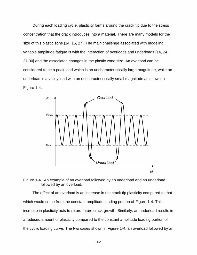
During each loading cycle, plasticity forms around the crack tip due to the stress
concentration that the crack introduces into a material. There are many models for the
size of this plastic zone [14, 15, 27]. The main challenge associated with modeling
variable amplitude fatigue is with the interaction of overloads and underloads [14, 24,
27-30] and the associated changes in the plastic zone size. An overload can be
considered to be a peak load which is an uncharacteristically large magnitude, while an
underload is a valley load with an uncharacteristically small magnitude as shown in
Figure 1-4.
Figure 1-4. An example of an overload followed by an underload and an underload
followed by an overload.
The effect of an overload is an increase in the crack tip plasticity compared to that
which would come from the constant amplitude loading portion of Figure 1-4. This
increase in plasticity acts to retard future crack growth. Similarly, an underload results in
a reduced amount of plasticity compared to the constant amplitude loading portion of
the cyclic loading curve. The two cases shown in Figure 1-4, an overload followed by an
max
N
min
Overload
Underload

26
underload and an underload followed by an overload result in different crack growth
paths and must be considered for an accurate analysis of variable amplitude fatigue.
Attempts to capture the behavior associated with the interaction between overload and
underloads has been explored through the use of empirical models such as crack
growth models [14, 27, 31-34], the small time scale model [24], the state-space model
[29, 30] in addition to elastic plastic fracture mechanics (EPFM) analysis in the FEM [35,
36] as well as the extended finite element method (XFEM) [37, 38].
Computational Fracture Mechanics
With the ever increasing speed of computers, numerical methods such as the finite
element method (FEM) are able to model problems with increasing fidelity and
increasing complexity, but finite element modeling of fatigue crack growth is still a
challenging computational fracture mechanics problem. As the finite element mesh must
conform to the geometry, the mesh around the crack tip must be recreated [25]
whenever growth occurs. Even if a concept such as crack-blocks [39] is used where a
small region around a crack tip is remeshed at each iteration, the computational
demands of the remeshing can contribute significantly to the simulations especially if a
large number of iterations of crack growth are to be modeled. In addition to the localized
mesh reconstruction around the crack tip, care needs to be taken to ensure accuracy in
the crack path, displacement, and stress intensity factors with FEM.
It is possible to model crack growth based on the cohesive zone model in the
classical FEM framework [40]. The cohesive zone model assumes that crack growth
can be represented as a traction-separation model as shown in Figure 1-5. Special
cohesive zone elements can then be used which allow for crack growth without the
need to remesh. However, some knowledge about the crack path is needed a priori in

27
order to define which elements in the mesh will be cohesive elements instead of
traditional methods. The model is based on the assumption that once the yield stress σY
is reached, the material properties start to degrade until some critical separation
distance δc is reached. At this point the given element/interface in the finite element
model can no longer sustain loading and fracture occurs.
Figure 1-5. Examples of possible traction-separation models that can be used as part
of a cohesive zone model where σY is the yield stress and δc is the critical separation.
The main challenge in cohesive zone models is to create an accurate model for
the given traction-separation relationship for a given material system including the
shape of the traction-separation model and the critical separation distance [40-42]. It is
often the case that the parameters of the traction-separation model for a given material
change according to the length scale in the model and corresponding experimental
tests. In practice, it can be the case that small changes to the parameters in the
traction-separation model result in substantial differences in the resulting finite element
solution [40]. Moody [41] introduced a series of experiments which can be used to
σ σ
σ
δ δ
δ
σY
σY σ
Y
σY
δc
δc
δc
δc
σ
δ

28
determine the traction-separation relationship. Scheider [42] explored the use of finite
element simulations to determine the traction-separation relationship. The shape of the
softening function that will be used to degrade the material properties is also of much
importance [40].
The XFEM [25] alleviates the challenges associated with the mesh conforming to
the geometry by allowing discontinuities or other localized phenomena to be
represented independent of the finite element mesh. Enrichment functions based on
linear elastic fracture mechanics (LEFM) are available which are independent of
material, unlike cohesive zone models, which are material and possible length-scale
dependent. Additional functions, referred to as enrichment functions, are introduced into
the displacement approximation through the property of the partition of unity [43].
Additional nodal degrees-of-freedom are also introduced that act to ‘calibrate’ the
enrichment functions as well as are used for interpolating within an element and in the
calculation of stresses or stress intensity factors using a method such as the domain
form of the contour integrals. While there is no need to worry about mesh construction
or the need to create a traction-separation relationship, the XFEM still requires the
convergence of the crack path, displacement, and stress intensity factors for accurate
crack modeling.
Scope
The goals and scope of this work are focused on accurate modeling of fatigue
crack growth under constant and variable amplitude loading for complex geometries
with unknown K a relationships with computational efficiency and high accuracy. In
particular the following topics are addressed:

29
Increasing the allowable step size for a given fixed increment of ∆a or ∆N without a
loss in accuracy when approximating the solution to the governing ordinary differential
equation for constant amplitude loading. The influence that this increased step size has
on the convergence of the crack path is also considered. A surrogate model is exploited
to enable the use of higher-order approximations to the calculation of magnitude and
direction of crack growth with a single expensive function evaluation. A variable step
size algorithm is also introduced to better allocate the available computational resources
based on the accuracy of the surrogate model when extrapolating.
The fundamental formulation of the XFEM is exploited to enable the modeling of
quasi-static crack growth with reduced computational time through an exact reanalysis
algorithm. When crack growth occurs, the changes to the global stiffness matrix are
limited to a localized number of elements about the crack tip. Here, a supernodal
Cholesky factorization is used to exploit these properties. During the first XFEM
simulation, the full stiffness matrix is formed and a Cholesky factorization is performed.
In all subsequent iterations this Cholesky factorization is directly modified to account for
the changes to in the stiffness matrix caused by crack growth. Computational savings
are realized for both the assembly and factorization of the global stiffness matrix. This
reanalysis algorithm is also employed as a means to consider optimization problems in
the XFEM framework where the location of a discontinuity is iteration dependent.
Multi-axial variable amplitude fatigue analysis is performed for the case where the
stress components are non-proportional. In this problem, traditional approaches based
upon ∆a or ∆N fail as the crack growth direction becomes cycle dependent. As the crack
path is unknown, the likelihood of having an analytical equation available for the stress

30
intensity factors as a function of crack size is small. Due to the variable amplitude
loading, the changing plasticity at the crack tip caused by the varying maximum and
minimum applied loads affects the crack growth rate. A test problem of an airplane wing
panel subjected to biaxial stresses during 19 flights based upon normalized flight data
from the Air Force Research Laboratory (AFRL) is considered. A method to scale and
convert the normalized data into equivalent biaxial loading cycles is given.
Outline
Chapter 2 introduces the level set method for tracking closed and open sections.
This method is used to track the location of discontinuities in the XFEM as they do not
conform to the mesh. This includes cracks, inclusions and voids. Chapter 3 introduces
the extended finite element method. First the general form is considered. Then
enrichment functions are introduced for cracks, inclusions and voids. A discussion of the
commercial and open-source implementations of XFEM is presented. Chapter 4 details
the domain form of the contour integral for the extraction of mixed-mode stress intensity
factors from a XFEM analysis of a cracked body. Criteria which determine the direction
of crack growth are introduced. Finally, fatigue crack growth models predicting the
magnitude of crack growth are given and limitations associated with these models are
discussed. In addition, rainflow counting methods are introduced for the purposes of
converting stress histories into equivalent stress cycles. Chapter 5 introduces the use of
a surrogate model for increased accuracy in the integration of the ordinary differential
equation governing fatigue crack growth allowing larger step sizes to be considered
without loss of accuracy for the case of constant amplitude loading. A surrogate model
may also be used to enable higher-order approximations to the crack growth direction.
An algorithm is also presented where the step size dynamically changes based on the

31
surrogate accuracy in order to minimize the number of finite element simulations
needed. Chapter 6 introduces and details the use of a reanalysis algorithm to make the
repeated simulations of crack growth in a quasi-static environment affordable, allowing
for additional simulations in a fixed amount of time. The sparse Cholesky factorization is
detailed as well as the algorithms which an be used to modify an existing sparse
Cholesky factorization. The proposed reanalysis algorithm leads to reduced
computational cost for repeated XFEM simulations. Chapter 7 details the variable
amplitude fatigue analysis procedure including the calculation of stress histories from
aircraft flight data, the conversion of these stress histories into cyclic loads which are
used in fatigue model prediction, and the prediction of crack growth under variable
amplitude loading using surrogate models and an exact XFEM reanalysis algorithm.
Chapter 8 summaries the research as well as suggesting possible areas of future work.

32
CHAPTER 2 THE LEVEL SET METHOD
Level Set Method for Closed Sections
The level set method was introduced by Sethian and Osher [44] as a numerical
method which can be used to track the evolution of interfaces and shapes. The method
is based on evolving an interface subjected to a front velocity given by the physics of
the underlying problem which is being modeled. Level set methods have been used in a
wide range of engineering applications in topics such as compressible [45] and
incompressible [46] flow, computer vision [47], image processing [48], manufacturing
[49-51] and structural optimization [52, 53]. While the figures given in this chapter are
two-dimensional, the principles can also applied to three-dimensional problems [54, 55].
The level set method is used to discretize the domain of interest into discrete
points. Each of these points is assigned a signed distance value from that point to the
nearest intersection with the interface denoted . A continuous level set function x
is introduced where x is a point in the domain of interest . The level set function can
be characterized as a function of the domain and with a time component as
, 0 for
, 0 for
, 0 for
t
t
t
x x
x x
x x
. 2-1
Thus, points inside the domain of interest are given negative signs, points outside of the
domain of interest are given positive signs, and points on the interface have no sign as
their signed distance is zero. An example of the signed distance function for a circular
domain is given in Figure 2-1. From Eq. 2-1 it can be noted that at any time t the
location of the interface can be found as the locations where

33
, 0 tx 2-2
and is commonly referred to as the zero level set of .
The evolution of the level set function is usually assumed to follow the Hamilton-
Jacobi equation [44] where the evolution can be predicted as
vt
2-3
where v is the front velocity and is the spatial gradient of the level set function. The
solution of Eq. 2-3 is usually approximated using finite differencing techniques [23]
which provide sufficient solution accuracy when the time step is small. When the
forward finite difference technique is considered, the derivative of with respect to time
can be approximated as
1 0
i ii i
tV 2-4
where 1 i is the updated level set value, i is the current level set value, iV is the front
velocity vector, and t is the elapsed time between i and 1i . Equation 2-4 can be
rewritten in a more convenient form in two-dimensions as
1
i ii i i it u v
x y 2-5
where iu is the front velocity in the x-direction and iv is the front velocity in the y-
direction. In Eqs. 2-4 and 2-5 the time step t is limited by the Courant-Friedrichs-Lewy
(CFL) condition [56] which ensures that the approximation to the solution of the partial
differential equation converges. The CFL condition is given as
max ,
max ,
x yt
u v 2-6

34
where x and y are the grid spacing in the x and y-directions. In practice, the level
set function needs to only be defined in a narrow band [57-59] around the interfaces of
interest or can be represented using the fast marching method [60], a variant of the
level set method with improved computational efficiency.
Figure 2-1. Example of a signed distance function for a closed domain.
Level Set Method for Open Sections
The version of the level set method presented in the previous section is only valid
for a closed section. For an open section, the definition of the interior, exterior, and
interface as defined in Eq. 2-1 no longer have a physical meaning. Stolarska [57]
introduced a modified version of the level set method which allows for open sections to
be tracked with the use of multiple level set functions. An open section as shown in
Figure 2-2 can be described by two level sets x and x . The interface of interest
is given as the intersection of x and x where
0 and 0 x x . 2-7
0 x
0 x
0 x

35
Figure 2-2. Example of the signed distance functions for an open section. (Note: the
interface of interest is given as the region where phi is negative and psi is equal to zero).
An updating algorithm for these two coupled level set function is also given by
Stolarska [57]. For the case of the x level set function, the update is identical to that
presented in Eqs. 2-3 - 2-5. Two regions are defined with respect to the x level set
function, update 0 x and no update 0 which correspond to the regions which will
and will not be updated. The level set function x is updated in two-dimensions
according to
1 no update
1 update
in
in
n n
i i
yn xi i i
F Fx x y y
F F
2-8
where the crack tip displacement vector is given as , x yF FF and the current crack tip
is given by the coordinates ,i ix y . The sign of the updated value 1 n
i is chosen to
correspond to the location of that node with respect to Figure 2-2.
0
0
x
x
0
0
x
x
0
0
x
x
0
0
x
x
0
0
x
x
0 x
0 x
0 x
0
0
x
x

36
Summary
The level set method allows for a closed or open section to be tracked by defining
signed distance values at discrete points in the domain of interest. The value of the level
set function at these points is then updated based on the front velocity at each point in
the domain using a finite difference technique to approximate the solution to the
governing partial differential equation. The CFL condition is used to ensure that the
solution of the differential equation converges. The level set method seems to be ideal
for use in a finite element environment where the nodes of the finite element mesh
could be used as the fixed points in the level set algorithm. The finite element shape
functions could be used to interpolate within an element to identify the values of the
level set function if this would be of interest.

37
CHAPTER 3 THE EXTENDED FINITE ELEMENT METHOD
General Form of the Extended Finite Element Method
The extended finite element method (XFEM) allows for discontinuities to be
represented independent of the finite element mesh by exploiting the partition of unity
finite element method [43] (PUFEM). In this method additional functions, commonly
referred to as enrichment functions, can be added to the displacement approximation as
long as the partition of unity is satisfied, i.e. N 1 I x for all x where NI x are the
finite element shape functions. The XFEM uses these enrichment functions as a tool to
represent a non-smooth behavior of field variables, such as stress across the interface
of dissimilar materials or displacement across cracks. In general, the enrichment
functions introduced into the displacement approximation are only defined over a small
number of elements relative to the total size of the domain. Additional degrees of
freedom are introduced in all elements where the discontinuity is present, and
depending upon the type of function chosen, possibly some neighboring elements which
are known as blending elements.
The additional functions used in the displacement approximation are commonly
called enrichment functions and the approximation takes the form:
N
h J J
I I I
I J
u x x u x a 3-1
where Iu are the classical finite element degrees of freedom (DOF), Jx is the Jth
enrichment function at the Ith node, and J
Ia are the enriched DOF corresponding to the
Jth enrichment function at the Ith node. The enriched degrees of freedom introduced by
Eq. 3-1 generally do not have a physical meaning and instead can be considered as a

38
calibration of the enrichment functions which result in the correct displacement
approximation. Note that Eq. 3-1 does not satisfy the interpolation property, h
I Iu u x ,
due to the enriched DOF, instead additional calculations are required in order to
calculate the physical displacement using Eq. 3-1. The interpolation property is
important in practice in applying boundary or contact conditions. Therefore, it is
common practice to shift [61] the enrichment function such that
J J J
I Ix x x 3-2
where J
I x is the value of the Jth enrichment function at the Ith node. As the shifted
enrichment function now takes a value of zero at all nodes, the solution of the resulting
system of equations satisfies h
I Iu u x and the enriched DOF can be used for
additional actions such as interpolation and post-processing operations. Here, the
shifted enrichment functions are referred to with upper case characters, and the
unshifted enrichment functions are referred to with lower case characters. The shifted
displacement approximation is given by
N
h J J
I I I I
I J
u x x u x a 3-3
where J
I x is the Jth shifted enrichment function at the Ith node. Hereafter, NI x
and J
I x will be written as N I and J
I .
The Bubnov-Galerkin method [62] may be used to convert the displacement
approximation given by Eq. 3-3 into a system of linear equations of form
Kq f 3-4

39
where K is the global stiffness matrix, q are the nodal DOF, and f are the applied
nodal forces. By appropriately ordering degrees of freedom, the global stiffness matrix
K can be considered as
uu ua
ua aa
T
K KK
K K 3-5
where uuK is the classical finite element stiffness matrix,
aaK is the enriched finite
element stiffness matrix, and uaK is a coupling matrix between the classical and
enriched stiffness components. The elemental stiffness matrix eK for any member of K
may be calculated as
d , u,a
h
T
eK B CB 3-6
where C is the constitutive matrix for an isotropic linear elastic material, uB is the
matrix of classical shape function derivatives, and aB is the matrix of enriched shape
function derivatives. The general form of uB and aB is given by
,
,
,
,
,,
u a
, ,, ,
, ,
, ,, ,
, ,
N 0 0
N 0 00 N 0
0 N 0
0 0 N0 0 N;
0 N N 0 N N
N 0 NN 0 N
N N 0
N N 0
J
I I x
JI xI I y
I yJ
I I zI z
J JI z I y
I I I Iz y
I z I x J J
I I I Iz xI y I x
J J
I I I Iy x
B B 3-7
where ,N I i is the derivative of NI x with respect to ix and ,
N J
I I i is the derivative of
N J
I Ix x with respect to ix . In practice, ,
N J
I I i is calculated with the product rule:

40
N N
N
J J
I I II J
I I
i i ix x x
x x xxx x . 3-8
Similarly, q and f in Eq. 3-4 are given by
TT q u a 3-9
where u and a are vectors of the classical and enriched degrees of freedom and
T T T u af f f 3-10
where u
f and af are vectors of the applied forces for the classical and enriched
components of the displacement approximation. The vectors u
f and af are given in
terms of applied tractions t and body forces b as
N d N d
h ht
u I If t b 3-11
and
N d N d
h ht
J J
a I I I If t b . 3-12
Stress and strain must be calculated with the use of the enrichment functions and
enriched degrees of freedom such that the effect of the discontinuity within a particular
element is considered. Therefore the strain and stress may be calculated as
T
u aε B B u a 3-13
and
σ Cε . 3-14
Enrichment Functions
The XFEM has been used to solve a wide range of problems involving
discontinuities. In general, discontinuities can be described as either strong or weak. A

41
strong discontinuity can be considered one where both the displacement and strain are
discontinuous, while a weak discontinuity has a continuous displacement but a
discontinuous strain. There exist enrichment functions for a variety of problems in areas
including cracks, dislocation, grain boundaries, and phase interfaces [63-66]. Aquino
[67] has also studied the use of proper orthogonal decomposition to incorporate
experimental data into the displacement approximation for cases with no logical choice
of enrichment function. Fries [68] introduced the use of hanging nodes in the XFEM
framework with respect to inclusions, cracks, and fluid mechanics to allow for
automated mesh refinement around discontinuities.
Crack Enrichment Functions
The modeling of cracks in the XFEM has been thoroughly explored [63-66, 69, 70].
Belytschko [71] was the first to study cracks in the XFEM framework based on the
element-free Galerkin crack enrichment of Fleming [72]. Moёs [25] introduced the use of
the Heaviside enrichment function to simplify the representation of the crack away from
the tip. Work has been done in two [25, 57, 71, 73, 74] and three-dimensions [54, 58-60,
75] for linear elastic [25, 54, 57-60, 71, 73-75], elastic-plastic [37, 76], and dynamic [77-
81] fracture.
The common practice is to incorporate two enrichment functions into the XFEM
displacement approximation to represent a crack. A Heaviside step function [25] is use
to represent the crack away from the tip and a more complex set of functions is used to
represent the crack tip asymptotic displacement field. The Heaviside step function is
given as
1, above crack
1, below crack
h x . 3-15

42
It can be noticed that the enrichment given by Eq. 3-15 introduces a discontinuity in
displacement across the crack. For a linear elastic crack tip, four enrichment functions
[72] are used to incorporate the crack tip displacement field into elements containing the
crack tip:
, 1 4
sin ,cos ,sin sin ,sin cos2 2 2 2
rx 3-16
where r and are the polar coordinates in the local crack tip coordinate system the
origin it at the crack tip and 0 is parallel to the crack. Note that the first enrichment
function in Eq. 3-16 is discontinuous across the crack behind the tip in the element
containing the crack tip, acting as the Heaviside enrichment does. Should a node be
enriched by both Eqs. 3-15 and 3-16, only Eq. 3-16 is used as shown in Figure 3-1
where the Heaviside and crack tip nodes are denoted by filled circles and squares.
Figure 3-1. The nodes enriched with the Heaviside and crack tip enrichment functions.
Elgeudj [37, 38] identified crack tip enrichment functions [37] which can be used to
capture the elastic plastic fracture behavior of the Hutchinson-Rice-Rosengren (HRR)
singularity [82, 83]. The HRR singularity is a model for confined plasticity in the fatigue

43
of power-law hardening materials. From a Fourier analysis three basis functions were
identified, and the basis with the lowest rank was chosen as the XFEM enrichment
function. These basis functions are given by
1 1
, 1 6sin ,cos ,sin sin ,cos sin ,sin sin3 ,cos sin3
2 2 2 2 2 2
nrx 3-17
where n is the power-law hardening exponent for the given material. Comparison
between the enrichment functions of Eq. 3-16 and Eq. 3-17 showed very similar
predictions in stress intensity factors between the elastic and elastic-plastic case for
several values of n . These crack tip enrichment functions were then implemented to
model elastic-plastic fatigue crack growth [38] for a material subjected to a combination
of overload and underload conditions with a very limited number of loading cycles. The
goal of this work was the capture the underlying plasticity evolution caused by the
interaction of overload and underloads. In benchmark problems the stress intensity
factor results do not show a significantly different prediction in stress intensity factor
over the traditional crack tip enrichment method, but require significantly more
computational resources for a given analysis. The similarity between the elastic plastic
and linear elastic cases is likely due to the confined plasticity about the crack tip during
fatigue crack growth. This was also observed by Anderson in the classical FEM [84].
Alternative crack tip conditions have also been explored such as bi-material cracks
[85], cohesive cracks [86-88], branching cracks [89], cracks under frictional contact [38,
90], fretting fatigue cracks [91], interfacial cracks [76, 85, 92, 93], cracks in orthotropic
materials [94], and cracks in piezoelectric materials [95]. Mousavi [96] introduced a
unified framework for the enrichment of homogeneous, intersecting, and branching
cracks through the use of harmonic enrichment functions. The XFEM has also been

44
used to study a variety of problems involving cracks including: the effect of cracks in
plates [97, 98], crack detection and identification [99-101], shape optimization [26], and
optimization with changing crack location using a reanalysis technique [22].
Because the XFEM mesh does not need to conform to the domain, a method must
be used to track of the location of the cracks. To this end the use of the open segment
level set method introduced by Stolarska [57] and detailed in Chapter 3 is used. Two
level set functions are used to track the crack, the zero level set of x represents the
crack body, while the zero level sets of x , which is orthogonal to the zero level set of
x , represents the location of the crack tips. The two enrichment functions given in
Eqs. 3-15 and 3-16 can be calculated in terms of x and x such that
1 for 0
1 for 0
h h
xx x
x. 3-18
Furthermore, the polar crack tip coordinates are given as
2 2 and arctan
r
xx x
x. 3-19
The enriched nodes corresponding to the crack tip enrichment can also be determined
through the use of the level set functions defining the crack. Consider an element where
the maximum and minimum values of x and x are given as max , min , max , and
min . Then an element is enriched with the Heaviside enrichment when
max max min0 and 0 3-20
and the crack tip enrichment when
max max min0 and 0 min . 3-21

45
Therefore, the extended finite element and level set methods complement one another
well for the tracking of the location of the cracks. The representation of cracks in three-
dimensions [54, 58, 60] follows a similar methodology. In practice the level sets are
defined in only a narrow band about the crack as discussed in Chapter 2 or the fast
marching method [54, 60] is used.
The convergence rate of XFEM with crack enrichment functions has been an area
of interest [65, 102-107], particularly with respect to the challenges presented by the
partially enriched or blending elements caused by the crack tip enrichment. No blending
issues exist with the Heaviside function as it vanishes along all element boundaries. It
was noticed by Stazi [104] that the convergence rate for the XFEM was lower than the
equivalent traditional finite element problem. Chessa [108] identified that the partially
enriched crack tip elements lead to parasitic terms in the displacement approximation
and introduced an enrichment dependent assumed strain model to increase the
convergence rate. Fries [102] introduced a linearly decreasing enrichment weight
function in the blending elements to increase convergence. An area [103, 109, 110]
instead of single element crack tip enrichment has also been shown to increase
convergence. Through the use of these methods the convergence rate of cracked
domains with the XFEM has become equivalent to the equivalent traditional finite
element problem [65, 102, 107].
Inclusion Enrichment Functions
The modeling of material interfaces independent of the finite element mesh
through the element-free Galerkin [111] as well as partition of unity finite element
method [55, 61, 63, 65, 66, 112-115] has been studied. The enrichment function should

46
incorporate the behavior of the weak discontinuity, i.e., continuous displacement, but
discontinuous strain. The Hadamard condition [113] given by
F F a n 3-22
where F is the deformation gradient, n is the outward normal material interface, and a
is an arbitrary vector in the plane. The Hadamard condition must be satisfied by the
chosen enrichment function.
Sukumar [113] first introduced the use of the absolute value enrichment in terms of
the level set function x , which gives the shortest signed distance from a given point
to the interface between the two materials. Therefore, the enrichment function takes the
form:
x x . 3-23
The enrichment function is assumed to be nonzero only over the domain of support for
the enriched nodes, as with the crack enrichment function. For a bi-material boundary-
value benchmark problem the absolute value enrichment given by Eq. 3-23 led to a
convergence rate which was lower than the equivalent traditional finite element method
problem where the mesh conforms with the material interface. It was hypothesized that
the poor convergence was related to the blending elements containing a partial
enrichment. In an attempt to improve the convergence rate a smoothing algorithm was
introduced to reduce the effects of the blending elements which increased the
convergence rate, but did not equal the traditional finite element method.
Moёs [55] studied modeling complex microstructure geometries with the use of
level set defined material interfaces and introduced a new enrichment function. The
modified absolute value enrichment takes the form:

47
N N I I I I
I I
x x x . 3-24
Note that the enrichment function given by Eq. 3-24 is zero at all nodes and thus, does
not need to be shifted such that traditional degrees of freedom are recovered
automatically. If an interface corresponds to the mesh, then no nodes are enriched as
the enrichment function will be zero and the problem will be equivalent to the traditional
finite element problem. The same benchmark problem considered by Sukumar [113]
was considered as well as a similar problem in three-dimensions. In two-dimensions the
convergence rate was shown to equal the traditional finite element method. In three-
dimensions the convergence rate was slightly less than the traditional finite element
method. This method is considered the current state-of-the-art for modeling inclusions
with the XFEM.
Pais [112, 115] considered an element-based enrichment instead of nodal
enrichment where the displacement approximation took the form
N h
I I e
I
u x x u x a 3-25
where x is a piecewise linear enrichment function where
0
0 1
I xx
x 3-26
and ea are elemental degrees of freedom. Thus, the enrichment function vanishes at all
nodes and takes a value of one at the interface locations. The proposed method allows
for the number of elemental degrees of freedom to be equal to the number of
dimensions of the problem. The resulting system of equations needs fewer degrees of
freedom than either the traditional or extended finite element method to represent the

48
same domain. It was found that the convergence rate is comparable to the absolute
value enrichment given by Eq. 3-23, due to errors in the prediction of the shear stress
distribution in two and three-dimensions. A comparison of the enrichment functions for
Eqs. 3-23-3-25 is given for the case of a bi-material bar shown in Figure 3-2. A
comparison of the enrichment functions and locations of the enriched degrees of
freedom for the absolute value, modified absolute value and element-based enrichment
functions is given in Figure 3-3.
Figure 3-2. One-dimensional bi-material bar problem.
Figure 3-3. Comparison of the various inclusion enrichment functions and locations of
the enriched degree(s) of freedom for a one-dimensional bar.
The problem given in Figure 3-2 can be solved using the absolute value
enrichment, modified absolute value enrichment, or element-based enrichment all of
x
L x0 0
0
1
y Absolute value
Element-based
Modified absolute value
Enriched DOF
Bar 1 P
0.25L 0.75L
Bar 2

49
which yield equivalent final answers. When additional elements are considered, the
smoothing of the absolute value enrichment presents a challenge not found with the
modified absolute value or element-based enrichment for recovering the theoretical
displacement. Due to the improved convergence rate for the modified absolute value
enrichment this method is the most popular approach in the literature for modeling
inclusions with XFEM. For the most part, continued work in the area of modeling
inclusions in the XFEM tends to application oriented instead of focusing upon the
development of enrichment functions which offer improved performance.
Other work on modeling inclusions in the XFEM include a unified model for the
representation of arbitrary discontinues and discontinuous derivatives [61]. The
imposition of constraints along moving or fixed interfaces was considered by Zilian
[114]. Dirichlet and Neumann boundary conditions for arbitrarily shaped interfaces were
presented for a general enrichment function. Instead of Lagrange multiplier [116, 117] or
penalty method [118] approaches, a mixed-hybrid method was introduced. Constant
boundary tractions, prescribed displacement differences and prescribed interfacial
displacement states were applied to a bi-material problem. Hettich [119, 120] studied
the modeling and failure of the interface between fiber and matrix in composite
materials.
Void Enrichment Function
Daux [89] was the first to represent voids with the XFEM. Sukumar [113] later
extended the void enrichment to take advantage of the use of the x level set
function to track the void. Unlike the other enrichment functions presented here, the void

50
enrichment function does not require additional DOF; instead the displacement
approximation for a domain with a hole takes the form
V N h
I I
I
u x x x u 3-27
where V x takes a value of 0 inside the void and 1 anywhere else. In practice,
integration is simply skipped where 0 x . Additionally, nodes whose support is
completely within the void are considered fixed DOF.
Integration of Element with Discontinuity
An area where the XFEM differs from the classical finite element method is on the
scheme used to perform the numerical integration of Eq. 3-6 as challenges arise in
elements which contain a discontinuity. Standard Gauss quadrature [23] requires that
the integrands are smooth, which is not the case for an element containing a strong or
weak discontinuity. The approach introduced by Moёs [25] was to divide a two-
dimensional element into a set of triangular subdomains, where the discontinuity was
placed along the boundary of one of the subdomains. Integration would then be
performed over each subdomain, resulting in a series of integrations over continuous
domains. The common number of gauss points for integration in each triangular
subdomain with the Heaviside enrichment is 3 while 7 are used for the crack tip
enrichment functions given in Eq. 3-16 [73]. An example of an element completely cut
by a crack as well as containing a crack tip and the associated subdomains for
integration are shown in Figure 3-4. The creation of the subdomains is straightforward
with the use of Delaunay tessellation for the nodal coordinates along with the
coordinates of the zero level set of x in the parametric space.

51
Figure 3-4. Elements containing a discontinuity and the continuous subdomains for
integration. A) element cut by crack, B) element cut by crack divided into four continuous subdomains, C) element containing crack tip, D) element containing crack tip divided into 5 continuous subdomains.
Elguedj [37, 38] introduced a hybrid integration method for the case of modeling
the evolution of plasticity of an elastic-plastic crack on a structured mesh. Elements
which were within a given radius around the crack tip were subdivided into 16 square
subdomains. Within each square subdomain, 16 gauss points were used in order to
track the evolution of plasticity within the model. As the crack evolved, all gauss points
associated with previous plasticity were updated and additional elements were divided
into subdomains according to crack growth. Note that 256 gauss points are used for an
elastic-plastic crack enriched element, while one would expect an average of 35 gauss
A
C
B
D

52
points for the case without plasticity. The implication is that in addition to solving a
nonlinear system of equations to capture the plasticity based on the HHR singularity
model, more gauss points will be used for a comparable simulation. This leads to a
computational problem which is much more demanding if plasticity is to be modeled
with XFEM.
In three-dimensions, it is possible to decompose elements cut by planar cracks
into a series of tetrahedrons [75] in a similar fashion to that of two-dimensional
elements. Mousavi also explored integration over arbitrary polygons [121] with an
application to XFEM [121] and through the use of the Duffy transformation [122],
showing excellent accuracy in the presence of singularities. Sukumar [123] presented a
method for the integration of an arbitrary polygon based on Schwarz-Christoffel
conformal mapping. Yamada [124] presented a hybrid numerical quadrature scheme
based on a modified Newton-Cotes quadrature scheme. Park [125] introduced a
mapping method for integration of discontinuous enrichments. Other methods are
detailed by Belytschko [63] and Fries [66].
XFEM Software
Due to the relatively short history of the XFEM, commercial codes which have
implemented the method are not prevalent. There are however, many attempts to
incorporate the modeling of discontinuities independent of the finite element mesh by
either a plug-in or native support [66, 126-129]. As most of these implementations are
works in progress there are various limitations on their practical use.
Abaqus®
In 2009, the Abaqus® 6.9 release [128] introduced basic XFEM functionality to the
Abaqus® CAE environment. The Abaqus® implementation of the XFEM is somewhat

53
different from that which was previously presented in this chapter. The implementation
is based on the phantom node method which was introduced by Hansbo [130] and
subsequently modified by Song [131] and Rabczuk [132]. The fundamental difference
between this implementation and the original XFEM is that the discontinuity is described
by superimposed elements and phantom nodes. In effect, an element is only defined in
an area where an element is continuous. Several elements are combined together such
that the total behavior of a discontinuous element is described. The method
implemented by Abaqus® considers a cohesive crack model, which is only enriched with
the Heaviside function given by Eq. 3-18. Note that it has been shown repeatedly that
the use of only the Heaviside enrichment leads to poor accuracy of the resulting J-
integral calculation [129]. As a result of this enrichment scheme, all enriched elements
must be completely cut by the crack, as no crack tip field is considered.
Some limitations with modeling crack growth within Abaqus® using the XFEM are:
Only the STATIC analysis procedure is allowed
Only linear continuum elements are allowed with or without reduced integration
No fatigue crack growth models are available
No intersecting or branching cracks are allowed
A crack may not turn more than 90° within a particular element
The Abaqus® 6.9: Extended Functionality [127] update allows for energy release
rate and stress intensity factors to be evaluated for three-dimensional cracked domain.
There is currently no method available for the extraction of stress intensity factors in
two-dimensions. In practice, the modeling of crack growth within Abaqus® with the
current implementation of the XFEM is challenging. As the formulation is based on the
cohesive model the same challenges exist of solving the system of equations as with

54
cohesive elements and methods such as viscous regularization must be applied to
solve the system of equations. Care must be taken to choose the regularization
parameters in a way that has a minimal impact on the resulting solution. The Abaqus®
6.10 [133] updated enables parallel processing of some XFEM simulations. The
Abaqus® 6.10: Extended Functionality [36] update enables low cycle fatigue predictions.
MATLAB® XFEM Code (MXFEM)
Basic functionality of the XFEM was implemented by Pais [134] in MATLAB® for
two-dimensional plane stress and plane strain problems. This code has been given the
name MATLAB® XFEM Code (MXFEM) rectangular domain may be defined with a
structured grid of linear square quadrilateral elements with arbitrary loading and
boundary conditions. Enrichments provided include the homogeneous [25] crack,
inclusion [55] and void [89, 113]. All discontinuities are tracked using the level set
method detailed in Chapter 3 and enrichment functions are calculated from level set
values as detailed previously in this chapter. The x and x level set functions
track the crack, the x level set function tracks the voids, and the x level set
function tracks the inclusions. Integration of enriched elements is done through
subdivision of elements into triangular regions [25, 73].
A variety of plotting outputs may be requested including: level set functions, finite
element mesh, deformed finite element mesh, elemental and contours of stress, and
stress-intensity factor history for growing cracks. A graphical user interface (GUI) is
available which offers simplified functionality compared to the direct modification of the
input file. The GUI writes an input file based on the values of the GUI and then solves
the problem. An example of the GUI is given in Figure 3-5. Examples of some of these

55
plots are given for the geometry shown in Figure 3-6, Figure 3-7, and Figure 3-8, which
contains a circular inclusion below the crack and a void above the crack.
The domain form of the contour integrals [18, 19] is used to calculate the mixed-
mode stress intensity factors. The mixed-mode stress intensity factors are used in the
critical plane approach [133] or the maximum circumferential stress criterion [18] to give
the direction of crack extension. Crack growth may be modeled using either a constant
increment of growth or a fatigue crack growth model, such as Paris model [34] or a
modified Paris model [14, 27] which considers the effects of variable amplitude loading.
Four models [133, 135-137] are available for the conversion of the mixed-mode stress
intensity factors into an equivalent stress intensity factor range. For the case of variable
amplitude loading a separate input file may be used to define the cycle-dependent
loading parameters for the two-dimensional state of stress. Either the forward Euler
method or surrogate models as presented in Chapter 4 can be used in the integration of
the fatigue model. Surrogate models are used through the use of the SURROGATES
Toolbox [138]. All crack growth problems are solved using the reanalysis algorithm
presented in Chapter 5.
Additional functionality includes an optimization algorithm for finding some
optimum crack location and the ability to define a variable load history. The code has
been prepared in an attempt to facilitate other models for crack growth direction,
equivalent stress intensity factor, and fatigue crack growth models. Benchmark
problems for the various enrichment functions are provided in Appendix A including:
crack, inclusion, and void enrichment functions, fatigue crack growth, and optimization
to identify the crack location with maximum energy release rate for a plate with a hole.

56
Figure 3-5. MXFEM GUI for automated input file creation.
A B
Figure 3-6. Example problem to show plots generated by MXFEM. A) The geometry being considered, B) Example of the mesh output from MXFEM where circles and squares denote the Heaviside and crack tip enriched nodes and the circles denote the inclusion enriched nodes.
H/4
H/4
H/4
H/4
a
r
r

57
A B C D
Figure 3-7. Example of the level set functions output from MXFEM. A) x , B) x ,
C) x , D) x .
A B C D
Figure 3-8. Example of the stress contours output from MXFEM. A) XX , B) XY , C)
YY , D) VM .
Other XFEM Implementations
Bordas [69] implemented the XFEM as a object-oriented library in C++. Cenaero
[139] has implemented XFEM functionality into the Morfeo finite element environment.

58
Giner [129] implemented the XFEM in Abaqus® with the traditional crack tip enrichment
scheme for modeling two-dimensional growth through the use of user defined elements.
Global Engineering and Materials, Inc. [126, 140] is developing a XFEM-based failure
prediction tool as an Abaqus® plug-in which includes a small time scale fatigue model
[24] for variable amplitude loading. Sukumar [73, 74] implemented the XFEM in Fortran,
specifically the finite element program Dynaflow®. Wyart [141] discussed the
implications of the implementation of the XFEM in general commercial codes. Some
amount of functionality is also available in getfem++ [142] and openxfem++ [143].
Summary
The XFEM allows for strong and weak discontinuities to be represented
independent of the finite element mesh by incorporating discontinuous functions into the
displacement approximation through the partition of unity finite element method.
Additional nodal degrees of freedom are introduced at the nodes of elements cut by a
discontinuity. An assortment of enrichment functions are available for a variety of crack
tip conditions and the Heaviside step function is used to model the crack away from the
tip. Elastic-plastic crack tip enrichment functions are available for materials which
power-law hardening based on the HHR singularity model. The stress intensity factor
results do not show a significantly different prediction in stress intensity factor over the
traditional crack tip enrichment method, but require significantly more computational
resources for a given analysis. Inclusions are modeled using the modified absolute
value enrichment, which shows convergence equivalent to that of the classical finite
element method. Voids can be incorporated through the use of a step function and
without additional nodal degrees of freedom. Integration of elements containing

59
enriched degrees of freedom, and therefore a discontinuity require special integration
treatment through the use of either a subdivision or equivalent algorithm.
As the discontinuities do not correspond to the finite element mesh, some other
method must be used to track the discontinuities. The level set method for open
sections is used to track any cracks in the domain. The level set method for closed
sections is used to track inclusions and voids. The level set values are used as part of
the definition of the enrichment functions, leading to a symbiotic relationship between
the extended finite element and level set methods.
A version of the XFEM for the modeling of cohesive cracks has been introduced in
Abaqus® 6.9, but it is not without its limitations. An implementation within MATLAB® had
been completed here. The XFEM is also available through the use of plug-ins or some
open source finite element codes.

60
CHAPTER 4 CRACK GROWTH MODEL
Stress Intensity Factor Evaluation
The most common way to extract the mixed mode stress intensity factors is
through the use of the domain form of the interaction integrals [16, 18, 19, 85] in two
[25, 73, 89] or three-dimensions [54, 59, 75]. The domain form of the interaction
integrals is an extension of the J-integral originally introduced by Cherepanov [144] and
Rice [17]. In the domain form, the line integral specified by the J-integral is converted to
an area integral which is much more amenable to use with finite element simulations.
As the J-integral is used to calculate the energy release rate for a given crack, the
interaction integrals are used to extract the mixed-mode stress intensity factors. This
method has been shown to have excellent accuracy when applied to suitable meshes
for many crack conditions including homogenous [25], bi-material [85], and branching
[89] cracks. Other methods [63, 64, 66] have also been explored in the literature.
For a general mixed-mode homogeneous crack in two-dimensions the energy
release rate G can be expressed in terms of the relationship between the J-integral,
stress intensity factors and effective Young’s modulus effE as
2 2
I II
eff eff
K KG J
E E 4-1
where effE is defined by the state of stress as
2
plane stress
plane strain1
eff
E
E E 4-2
where E is Young’s modulus and is Poisson’s ratio. The J-integral takes the form

61
1
1
d
kjk j
uJ Wn n
x 4-3
where W is the strain energy density. Equation 4-3 can be rewritten in the equivalent
form using the Dirac delta which is easier to implement in finite element code as
1
1
d
ij ij j
uJ W n
x. 4-4
In order to calculate the mixed-mode stress intensity factors, two displacement
and stress states are superimposed onto one another. Auxiliary stress and
displacement states are superimposed onto the stress and displacement solution from
XFEM. The auxiliary stress and displacement states at the crack tip introduced by
Westergaard [145] and Williams [146] for a homogenous crack and by Sukumar [85] for
a bi-material crack are used in the calculation of the mixed-mode stress intensity
factors. The auxiliary stress and displacement states for a homogeneous crack are
given in Appendix B. Hereafter, the XFEM states are given as 1
iju , 2 ij , and 2
ij while
the auxiliary states are given as 2
iju , 2 ij , and 2
ij . The superposition of stress states
into Eq. 4-4 leads to
1 2
1 2 1 2 1 2 1 2
1
1
1d
2
i i
ij ij ij ij j ij ij j
u uJ n
x. 4-5
The expansion of the terms of Eq. 4-5 allows for the J-integral to be separated to the
auxiliary state 2J , XFEM state 1
J , and interaction state 1,2I given by
2 1
1,2 1,2 1 2
1,
1 1
d
i ij ij ij j
u uI W n
x x 4-6
where 1,2W is the interaction strain energy density given as

62
1,2 1 2 2 1 ij ij ij ijW . 4-7
The two superimposed stress states can be expressed using Eq. 4-1 after
rearrangement as
1 2 1 2
1 2 1 22
I I II II
eff
K K K KJ J J
E. 4-8
Therefore, from Eqs. 4-6 and 4-8, the interaction state is given as
1 2 1 2
1,22
I I II II
eff
K K K KI
E. 4-9
The stress intensity factors for the XFEM state 1
IK and 1
IIK are given by selecting
21IK and 2
0IIK , followed by 20IK and 2
1IIK such that 1
IK and 1
IIK are:
1,Mode
1
2
I
eff
I
I EK 4-10
where 1,Mode II is the interaction integral for 2
1IK and 20IIK and
1,Mode
1
2
II
eff
II
I EK 4-11
where 1,Mode II is the interaction integral for 2
0IK and 21IIK .
The interaction integral in Eq. 4-6 is converted from a line integral into an area
integral and a smoothing function sq which takes a value of 1 on the interior of the line
integral defined by Eq. 4-6 and a value of 0 outside of the integral. Elements for the
integration are selected by choosing a radius from the crack tip. When this radius
becomes sufficiently large the integral becomes path-independent; i.e., any path larger
than the path-independent radius indr will yield equivalent solutions to Eq. 4-6. In practice

63
a radius of three elements about the crack tip is typically sufficient for path-
independence. An example of the elements contained within a given radius from the
crack tip is given in Figure 4-1. The divergence theorem is used to create the equivalent
area integral
2 1
1,2 1 2 1,2
1
1 1
d
i i s
ij ij jA
j
u u qI W A
x x x 4-12
which is simpler to implement in the finite element environment.
Figure 4-1. The elements within a specified radius for path-independence. A) Radius of
three elements, B) Radius of 5 elements.
Other methods have also been used to extract the mixed-mode stress intensity
factors using XFEM. Duarte [147] used a least squares fit of the localized stress state
around the crack tip to extraction the stress intensity factors. Karihaloo [64] included
higher-order terms of the asymptotic crack tip expansion in two-dimension which
allowed for the stress intensity factors to be obtained directly without the use of
interaction integrals. No equivalent extension has been performed in three-dimensions
[63]. Lua [126, 148] introduced nodes along the crack fronts which were used with the
crack-tip opening displacement [15] to calculate the mixed-mode stress intensity factors.
A B

64
Recall that the crack-tip opening displacement approach for finding stress intensity
factors is only valid for linear elastic cracks. Sukumar [60] attempted to evaluate the
stress intensity factors directly from the enriched degrees of freedom corresponding to
the crack tip enrichment function for pure mode I problem, but the accuracy of the stress
intensity factors was found to be insufficient. A similar method was introduced by Liu
[149] with much better results for homogeneous and bi-material cracks.
Crack Growth Direction
The direction of crack propagation is accepted to be a function of the mixed-mode
stress intensity factors present at a crack tip. While there are several criteria available
for both two [21, 133, 150-153] and three-dimensions [133, 153], in general they only
differ in the angle of the initial kink, but then converge to similar crack paths [73]. In two-
dimensions, these methods tend to give the angle of crack extension, which in general
is the direction which will minimize IIK .
In two-dimensions the main criteria for the crack growth direction are the critical
plane approach [133], maximum circumferential stress [151], maximum energy release
rate [152] and the maximum strain energy density criterion [21]. Other criterion available
in the literature are the criterion of energy release rates and the generalized fracture
criterion [153]. The criterion which is most amenable to modeling crack growth with finite
elements is the maximum circumferential stress, as the growth direction c is given in a
closed form solution in terms of the mixed-mode stress intensity factors. The maximum
circumferential stress criterion [153] is given as the angle c given by
2 2 2
2 2
2 8arccos
9
II I I II
c
I II
K K K K
K K. 4-13

65
Alternative, but equivalent formulas are given by Moёs [25] as
2
12arctan 8
4
I Ic II
II II
K Ksign K
K K 4-14
and Sukumar [73]
2
22arctan
1 1 8
II I
c
II I
K K
K K
. 4-15
The critical plane approach [133] predicts that crack growth will occur along the
angle specified by as shown in Figure 4-2 for mixed-mode I and II loading as
4-16
where the angles and are
21
arctan2
II
I
K
K 4-17
and
2 2 2
2 2
2 4 4 1/ 3 5 1/ 41arccos 1
2 2 5 1/ 4
0 1
s s ss
s s
s
. 4-18
The parameter s is the ratio of the Mode I and II crack growth rates as
,d /d1
1 ,d /d
II a N
I a N
Kts
f K 4-19
where ,d /dI a NK and ,d /dII a NK are the stress intensity factors corresponding to a given
crack growth rate d / da N . The critical plane approach has the benefit of matching the
observations of Feng [154] where the crack paths were different for equivalent
magnitude loads in the axial and torsion directions.

66
Figure 4-2. Orientations of the critical and maximum normal stress planes.
There are two options available for determining the direction of crack growth, the
maximum circumferential stress and the critical plane approach. One difference
between these two methods is that the critical plane approach considers the effect of
the chosen material in addition to the current stress intensity factors through the use of
the Mode I and II threshold stress intensity factors, which may not be available for many
materials. Due to the simplicity of the maximum circumferential stress criterion and it's
acceptance in the XFEM literature [22, 57, 69, 71, 74, 86, 90, 129, 155], it will be the
preferred method for determining the crack growth direction.
Crack Growth Magnitude
At each cycle of constant amplitude fatigue, the amount of crack growth may be on
the order of nano-meters. In practice, the governing differential equation in Eq. 1-1 is
solved at discrete points, which will be referred to as simulation iteration in this work.
There are two main approaches presented in the literature for the amount of crack
growth at a given simulation iteration for constant amplitude loading. The first method
assumes that a known and finite amount of growth will occur at a given iteration. The
second method assumes that some governing law, such as a fatigue crack growth law
can be used to find the corresponding increment of growth at a particular iteration. For
x
y
α
β
γ
Critical plane
Maximum normal
stress plane

67
the case of variable amplitude loading with an unknown correction factor model for the
given crack geometry, the approaches used for constant amplitude loading are no
longer valid and each cycle must be modeled in order to predict the magnitude and path
of crack growth.
Finite Crack Growth Increment for Constant Amplitude Loading
In the literature, the selection of a constant crack growth increment is very popular
[22, 57, 69, 71, 74, 86, 90, 129, 155]. At a given cycle the amount of crack growth is
generally very small, approximately on the order of 10-8. Therefore, it is more
computationally attractive to choose a small increment of growth to represent many
cycles instead of modeling them independently. The choice of a is almost always
made a priori. It has been shown in the literature by Moёs [25], Pais [22] and Edke [26]
that the path of crack growth is related to the assumed increment. As the crack growth
increment is reduced, crack path convergence can be observed. The convergence of
crack path has also been related to the mesh density in the vicinity of the crack [22, 26].
Challenges with this method include selecting a a such that the crack path
converges to the appropriate path. With a single analysis it is unclear how one can
know whether or not the predicted crack path has converged. It is also unclear how to
interpolate between the data points since the a N crack growth curve is nonlinear.
Direct Fatigue Crack Growth
The slow progressive failure of a structure caused by crack growth under cyclic
loading is called fatigue. There are many fatigue crack growth models of varying
complexity [14]. Most fatigue crack growth models are of the following form:
d
,d
a
f K RN
4-20

68
where da/dN is the crack growth speed, K is the stress intensity factor range, and R is
the stress ratio. Many different models attempt to consider the effects of phenomenon
[14] such as crack growth instability when the stress intensity factor approaches it’s
critical value, threshold stress intensity factor, changing crack tip geometry, and elastic
crack tip conditions. For a variable load history, the interactions between overloads and
underloads are a crucial component of any fatigue crack growth model. An overload is a
load which is substantially greater than the mean, while an underload is a load which is
substantially less than the mean. Overloads increase crack tip plasticity which leads to
less crack growth in resulting loading cycles. An underload has the opposite effect and
leads to increased growth. The interaction of an overload and underload in subsequent
cycles is not well understood. Recent work such as the state-space model [29, 30],
small time scale model [24], and further modifications to fatigue models [14, 27] has
resulted in better predictions of fatigue crack growth under variable amplitude loading.
Classical Paris model
The first fatigue model was presented by Paris [34] and will be referred to here as
the classical Paris model. The relationship between the crack growth rate and the stress
intensity factor range is given as
d
d ma
C KN
4-21
where C is the Paris model constant, K is the stress intensity factor range, and m is
the Paris model exponent. The Paris model constant and exponent depend upon
material properties and loading conditions which can be derived from fatigue testing
data and are functions of the stress ratio R [156].

69
The classical Paris model given by Eq. 4-21 has limitations in its ability to model
fatigue crack growth. Research has shown that for a given material there is a minimum
stress intensity factor range which is required to cause crack growth which is commonly
referred to as the threshold stress intensity factor range thK [14, 27, 157]. Crack
closure [14, 28, 32] has been shown to be an important quantity to consider when
modeling fatigue failure , but is not a part of the classical Paris model. The classical
Paris model does not consider the applied stress ratio R which is the ratio between the
minimum and maximum load for a given cycle [14, 27, 31, 33]. Therefore, for the case
of variable amplitude loading where the stress ratio R is a function of the cycle number,
each cycle would need its own value of C and m. For the case of loading which is
variable in nature, the interaction between over-loads and under-loads is also not
considered as no variable is used which considers the interaction between loading
cycles.
Modified Paris model
One fatigue model which attempts to capture the behavior which is not part of the
classical Paris model is a modified version of the Paris model introduced by Xiaoping
[27] which will be subsequently referred to as the modified Paris model. Three additional
parameters are added to the classical Paris model; thK which accounts for the
threshold stress intensity factor range, RM which accounts for the stress ratio effect,
and PM which accounts for the interaction between over-loads and under-loads. The
modified Paris model takes the form
d
d
m m
R P th
aC M M K K
N 4-22

70
where C and m are the same material properties for the classical Paris model. The
value of the stress ratio correction factor RM is given as
1
2
1 5 0
1 0 0.5
1.05 1.4 0.6 0.5 1
R
R R
M R R
R R R
. 4-23
The values of and 1 are found by calibrating fatigue data curves from several stress
ratios such that they follow the same trend as is shown in Figure 4-3.
Figure 4-3. The use of the stress ratio correction factor MR to condense the various
stress ratios R into a single curve corresponding to R = 0 [27]. A) Fatigue data for some stress ratios R, B) Condensed fatigue data through the use of MR.
The value of pM is calculated as a function of the load interactions as
1
n
y
y OL OL
p OL OL i
y OL OL
ra r a r r
M a r a r
a r a r r
4-24
where yr is the plastic zone radius at the beginning of the cycle, OLa is the crack length
when the overload occurs, OLr is the plastic zone radius when the overload occurs, ia is
A ΔK MRΔK B
R = -1.0
R = 0.0
R = 0.3
R = 0.5
R = -1.0
R = 0.0
R = 0.3
R = 0.5
da/dN da/dN

71
the characteristic crack length for the ith cycle, r is the change in plastic zone size
caused by load interactions, and n is a shaping exponent determined by fitting to
experimental data of overload and underload cases. These plastic zones are shown in
Figure 4-4 where diameters are shown instead of radii.. The plastic zone sizes follow
2 2 2max
; ;
OL
uI Iy OL
y y y
KK Kr r r 4-25
where is a plastic zone size factor, max
IK is the maximum stress intensity factor for
the ith cycle, OL
IK is the stress intensity factor when the overload occurs, uK is the
interaction between loads given as min min
1 u I IK K K ,
y is the tensile yield stress of the
material, and
y is the compressive yield stress of the material.
Figure 4-4. The plastic zone and crack sizes which are used in the modified Paris
model to account for the effect of crack tip plasticity during load interactions.
The modified Paris model [27] has been validated for a variety of over-load, under-
load, and combinations of over-load and under-load cases as well as variable amplitude
aOL
ai
dOL
dy dΔ
Overload plastic zone, dOL
Overload-underload plastic zone, dOL-dΔ
Current plastic zone, dy

72
loading [27] showing improved agreement with experimental results compared to
AFGROW [35] and FASTRAN [84] models and comparable agreement with the state-
space model [29, 30]. While the modified Paris model proposed by Xiaoping [27] does
not directly contain a crack closure model, the effects of crack closure are approximated
by the tracking of plasticity associated with the interaction between the load cycles.
Equivalent Stress Intensity Factor
In order to apply the classical Paris model to mixed-mode loading, several
relationships have been proposed for the calculation of a single effective stress intensity
factor range which can be used in Eq. 4-21. Tanaka [136] proposed the relationship
4 44 8 eq I IIK K K 4-26
based on curve fitting observed experimental data. Yan [137] proposed a different
correction from the maximum circumferential stress criterion as
1
cos 1 cos 3 sin2 2
eq I IIK K K 4-27
where is given by Eqs. 4-13-4-15. Finally, a relationship based on energy release rate
[135] is given as
2 2 eq I IIK K K . 4-28
Liu [133] proposed a variety of equivalent stress intensity factors for any
combination of Mode I, II, and III loading based upon the critical plane model. For the
case of mixed-mode I and II loading the equivalent stress intensity factor is given as
2
2 221
1
eq H
kK k A k
B s 4-29
where k1, k2, and kh are related to the given mixed-mode stress intensity factor values as

73
1 1 cos 2 sin 22
I
II
Kk K , 4-30
2 sin 2 cos 22
III
Kk K , 4-31
and
3
IH
Kk . 4-32
The angle in Eqs. 4-30 and 4-31 is calculated from the angle defining the critical
plane as given by Eqs. 4-16 - 4-19. Finally, the constants A and B are found from the
value of s from Eq. 4-19 as
2
0 1
9 1 1
sA
s s, 4-33
and
2 2 2cos 2 sin 2 1
1
s sB
s s. 4-34
The choice of an equivalent stress intensity factor model is not a trivial task. The
models based on the energy release rate and proposed by Tanaka do not require any
information about the direction of crack propagation. Of these models, only the model of
Liu considers and accounts for the effects of failure due to shear or tension according to
the underlying model parameters. Therefore, this model will be the preferred choice.
Integration of Fatigue Crack Growth Model
For an arbitrary differential equation of the form ' ,y x f x y x the goal is to
predict the value of 1iy while the current data is available up to iy . The simplest
numerical method available which is applicable to the current crack growth problem is
the explicit forward Euler method [23] given as

74
1 , i i i iy y hf x y 4-35
where h is the step size from ix to
1ix . Note that ,i if x y is the slope of y x at ix ;
therefore a linear approximation is being made from ix to
1ix using the slope at the ix .
This method has been popular in engineering applications because it only requires
evaluating the slope at the current step, which often required expensive computational
simulation. For example, in the case of crack growth simulation, ,i if x y corresponds
to calculating the stress intensity factor with given crack size iy . Therefore, evaluating
,i if x y requires a finite element modeling with the current geometry of the crack. If a
different method, such as the backward Euler method, is used, then 1 1, i if x y is
required, which is the stress intensity factor corresponding to the unknown crack size
1iy . Therefore, there exists a fundamental difficulty to use a numerical integration
method other than the forward Euler method.
The simplest approach to integrating the Paris model for fatigue crack growth is
the use of the forward Euler method. Here the stress intensity factor range at the current
crack geometry is the only information needed to find the increment of growth between
the current and future crack geometries. The growth increment is calculated as
m
i ia N C K 4-36
where i is the current increment. The corresponding number of elapsed cycles can be
approximated as
i m
i
aN
C K 4-37

75
for a fixed increment of crack growth. As the forward Euler method only uses the slope
at the current point and linearly interpolates to the next crack size it can lead to large
inaccuracies for relatively small crack growth increments. Although the physical
meaning of N is the number of elapsed cycles, in this model it is treated as a
continuous variable as crack growth occurs over tens of thousands of cycles. Choosing
a larger N results in needing fewer finite element simulations while sacrificing
accuracy.
Although the forward Euler method can resolve the issue related to evaluating the
slope at unknown crack sizes, it has a drawback in slow convergence; the accuracy of
the method is proportional to the step size, h. In crack growth analysis, the step size
represents the number of fatigue loading cycles between two evaluation points. Since
cracks grow slowly throughout the lifecycle of a product, a small step size means tens of
thousands of simulations. Therefore, it is highly desired to use a numerical integration
method that allows a larger step size, while maintaining accuracy.
There are numerous numerical methods that allow larger step sizes for integration,
but the midpoint integration method is used as a demonstration tool in this paper. The
midpoint method [23] generally provides a better accuracy than the forward Euler
method as it takes the slope at the midpoint between the current and future data points
1/2ix and uses that value to approximate the interval from ix to 1ix such that
1 1/2,2
i i i i
hy y hf x y . 4-38
As it is rare for 1/2iy to be evaluated directly, 1/2iy it can be approximated as
1 , ,2 2
i i i i i i
h hy y hf x y f x y . 4-39

76
The accuracy of the method is proportional to h2; therefore, it allows a larger step size
for the same accuracy with the forward Euler method. While the midpoint approximation
specifies a crack length for the evaluation at the midpoint location, no direction is
specified. For a mixed-mode crack growth problem, the direction of crack growth can be
approximated based upon the first required function evaluation at ,i if x y . This may
limit the choice of integration step size however, as in effect an Euler approximation is
used for the crack growth direction while a higher-order approximation is used for the
crack growth magnitude.
In terms of integrating the Paris model is the use of the midpoint method where the
growth increment is calculated as
1/22
mmm
i i i i
Na N C K N C K a C K a 4-40
where 1/ 2i is the midpoint between the current and next increment. Similarly, iN is
given as
1/2
2
i m m
i ii
a aN
C K aC K a
. 4-41
Here the slope at the midpoint of the current cycle is use to extrapolate ahead to 1i .
This leads to a better approximation of the crack size at the next increment as a more
accurate approximation of the slope over the entire interval of the chosen growth
increment is used. This method requires additional function evaluations at 1/ 2i for
each crack geometry, effectively doubling the number of function evaluations needed for
the given simulation.

77
With regards to the XFEM, crack growth models have been limited primarily to the
Paris model and modeling in terms of the crack growth increment a . Belytschko [61]
used it to drive the crack growth for a plate with holes, but no specifics about how the
classical Paris model was used is given. Gravouil [58] coupled the level set method to
the classical Paris model, but no clear definition of the number of elapsed cycles was
given. Instead the growth was governed by assuming N to be equivalent to the
traditional time for the level set method. Sukumar [60] calculated the increment of crack
growth a as
max
max
m
I
I
Ka
a K 4-42
where maxa was taken as 00.05a for initial crack length 0a for a value of max
IK
corresponding to the maximum value of IK along the crack front. Note that here a value
for maxa acts very similarly to that of a fixed a such that a small value is required to
ensure convergence.
Example problem
An example is provided here where an XFEM analysis was performed on a plate
with a hole as shown in Figure 4-5. The chosen plate dimensions were a width of 4 m
and a height of 8 m with a hole with radius 1 m centered at (2,2) m. The edge crack has
an initial length of 0.5 m. The material properties for the plate were chosen as Young’s
modulus of 10 MPa, Poisson’s ratio of 0.33, Paris model constant and exponent of
1.5·10-10 and 3.8 respectively. The applied stress was 14.5 MPa. The purpose of this
study was to attempt to assess the effect that the mesh density and crack growth
increments a and N on the predicted crack path as shown in Figure 4-6.

78
Figure 4-5. Plate with a hole subjected to tension to examine the effects of mesh
density, crack growth increment, and number of elapsed cycles upon the convergence of crack path. A) Geometry, B) Example mesh.
Figure 4-6. Convergence of crack path as a function of the mesh density, crack growth
increment, and number of elapsed cycles. A) Mesh density, B) a, C) N.
From Figure 4-6 it is clear that the choice of mesh size is very important as
expected. Without a sufficiently refined mesh, the accuracy of the stress intensity
factors will be poor leading to an inaccurate prediction of the crack growth direction. The
crack path is relatively insensitive to the choice of a in this choice, but there is
deviation between the steps if a close up image of the crack paths near the hole is
A B C
h = 1/5
h = 1/10
h = 1/20
Δa = 1/10
Δa = 1/20
Δa = 1/40
ΔN = 50
ΔN = 25
ΔN = 1
σ
σ
a
A B

79
examined as in Figure 4-7. The most sensitive case is that of N where the cases of
N = 25, and 50 cycles actually miss the hole as predicted by N = 1. This reinforces
the observations that the direct solution of a fatigue crack growth model is very sensitive
to the choice of mesh, and crack growth increment.
Figure 4-7. Close up view of the crack paths for a around the hole.
Cycle Counting Methods
In the life estimation of a given structure it is necessary to convert the history of a
given loading parameter for a given structure into cycles which allow for the application
of a fatigue crack growth model. For structures which experience constant amplitude
loading with a constant mean stress over the loading history, this is a trivial task.
However, for a structure where the mean and amplitude of loading are non-constant it is
more challenging to determine what portion(s) of the given load parameter correspond
with a single cycle of loading. This loading parameter can be any parameter of interest
such as but not limited to acceleration, deflection, force, strain, stress, or torque.
Cycle counting methods do not consider the effect of the loading sequence when
converting a given loading parameter into an equivalent cyclic history for the same
Δa = 1/10
Δa = 1/20
Δa = 1/40

80
parameter. For many high-cycle fatigue applications, the loading sequence does not
significantly affect the prediction of damage accumulation from a fatigue damage model
instead of a fatigue crack growth model [158]. For the case of variable amplitude
fatigue, it has been established that the order of loading has an effect on the crack
growth prediction due to the changes in the plastic zone size caused by variable
amplitude fatigue, however, including the plasticity in the evaluation of the stress
intensity factors has little difference from the LEFM solution [37, 38, 159].
There are many methods available to attempt to convert a loading history into a
cyclic history such as level crossing cycle counting, peak-valley cycle counting, range
counting, range-pair method, and rainflow cycle counting method [160-165]. Of these
methods, the focus here will be upon the use of the rainflow counting method where
stress is the loading parameter of interest. To this end, the MATLAB® code rainflow by
Nieslony [166, 167] which follows ASTM E 1049, Standard Practices for Cycle Counting
in Fatigue Analysis is used to convert a given stress history into a series of cyclic loads.
For the case of non-proportional multi-axial stress histories the common practice is
to first convert the multi-axial stress components (e.g. xx , yy , and xy for two-
dimensional stress) into a single equivalent stress eq . In order to convert the multi-axial
stress components into a single equivalent stress there are methods based upon
approaches such as the critical plane method [158, 159, 168-170] or the Wang-Brown
method [171, 172]. This equivalent stress is then used in coordination with some fatigue
damage model such as
for 1, ,
i
ii
f
nD i k
N 4-43

81
where iD is the amount of damage at cycle i,
in is the number of cycles for a given
applied load, k is the total number of loading cycles, and if
N is the number of cycles to
failure at the same applied load. The cumulative damage iC at cycle i is given as
1
for 1, ,
i
i j
j
C D i k . 4-44
It is commonly assumed that once iC = 1, a given structure is fully damaged, can no
longer carry load, and has failed [15]. The fatigue damage model approach serves as
the basis for the identification of cycles from multi-axial stress data.
For a two dimensional analysis, the equivalent biaxial stress [173] for use in a
fatigue damage model can be calculated from
2 2 2 23 eq xx yy xx yy xy . 4-45
This equivalent stress can be used to identify the equivalent cyclic loading history. In
effect, for a fatigue damage model, once the equivalent stress eq has been calculated,
the bi-axial stress components (e.g. xx , yy , and xy ) can be discarded as they will no
longer be used. This is not the case here as the biaxial stresses are directly applied.
For variable amplitude fatigue, the interaction of the biaxial stresses will affect the
magnitude and direction of crack growth and should be applied directly to a cracked
plate. If a rainflow counting approach is applied to the individual stress components, it is
likely that each component will have a different number of cycles. The biaxial stress
components will be applied to a cracked plate in order to calculate IK and IIK . Before
the fatigue crack growth model can be directly applied, the stress history is converted
into an equivalent cyclic stress history. First, the equivalent biaxial stress is calculated

82
by Eq. 4-45. These cycles will then be superimposed upon the individual stress
components. This approach is detailed in Figure 4-8 where the conversion of the biaxial
stresses to an equivalent stress, the rainflow counting of that equivalent stress, and the
superposition of that equivalent stress onto the individual stress components is shown.
Figure 4-8. The strategy used to convert the bi-axial stress data into cyclic stress data
which was suitable for use in a fatigue crack growth model.
An unexpected result of this procedure was that the ratio of xx , xx , and xx are
typically different at the peak and valley of a given cycle. This creates a need for two
function evaluations, one at the maximum equivalent stress and one at the minimum
equivalent stress for a particular loading cycle, to be conducted in order for the stress
Calculate Equivalent
Stress
Rainflow
Counting
Data Cycle
Data
Data
Cycle
Cycle
Cycle Data
xx
xy
yy
vm vm
xx
xy
yy
Superimpose
Cycles
1
2
5
6
3
4
1 2
5
6 3
4
1 2
5
6
3
4
1
2 5
6
3
4

83
intensity factor range to be calculated. It should be noted that while the individual stress
components are being applied instead of the equivalent stress directly, the same cycles
are being followed which were identified according to the equivalent stress.
Summary
Crack growth is modeled using mixed-mode stress intensity factors which are
extracted from XFEM analysis with the use of the domain form of the contour integrals.
Four models are given for the direction of crack growth based upon the mixed-mode
stress intensity factors. The most popular of these models in the computational fracture
mechanics community is the maximum circumferential stress criterion. For cases where
shear may be a significant source of failure the Liu model may provide a better match to
experimental data.
Two of the many fatigue crack growth models are introduced, the classical Paris
model and a modified Paris model which has additional parameters to consider the
effects of the stress ratio R , threshold stress intensity factor thK , and changes in the
crack growth rate caused by the evolution of the plastic zone ahead of the crack tip
under variable amplitude loading. Four models are presented for the calculation of an
equivalent stress intensity factor range from the mixed-mode stress intensity factors.
The model proposed by Liu will be used here based upon it's superior performance
when compared to a range of experimental data for failure caused by shear and
tension.
The challenges with solution of a fatigue crack growth model were highlighted by
an example of fatigue crack growth in a plate with an edge crack an a hole. The effects

84
of mesh density, crack growth increment, and the elapsed number of cycles were
considered with respect to the convergence of the crack propagation path.
Finally, the rainflow counting method was introduced for the conversion of stress
histories into equivalent cycles. As these models are usually used for fatigue damage
prediction instead of direct fatigue crack growth modeling, the steps which are used in
the identification of cyclic stress histories for the biaxial stresses is detailed. First, the
equivalent biaxial stress is calculated. Cycles for the equivalent biaxial stress are
calculated according to the rainflow counting method. These cycles are then
superimposed upon the biaxial stresses, allowing for the biaxial stress components to
be applied directly for the analysis of a cracked plate subjected to variable amplitude
biaixal loading.

85
CHAPTER 5 SURROGATE MODELS FOR HIGHER-ORDER INTEGRATION OF FATIGUE CRACK
GROWTH MODELS
Integration of Ordinary Differential Equation
The objective of this chapter is to use a surrogate model to reduce the number of
expensive function evaluations needed in the numerical integration of an ordinary
differential equation which follows the general form
d
,d
yf x y
x . 5-1
For an unknown function f(x,y) a common method to approximate the solution is to
discretize f(x,y) into discrete points, where f(x,y) is approximated using some numerical
technique. In this work, finite element simulations are used to approximate f(x,y). There
are numerous methods available to approximate the solution to Eq. 5-1 at some 1iy
from some current state iy , such as the forward Euler approximation which is
1 ,i i i iy y hf x y 5-2
where h is the integration step size given as xi+1-xi or the midpoint approximation as
1 1/2 , ,2
i i i i i i
hy y hf x y f x y
. 5-3
The midpoint approximation allows for larger step sizes h to be taken compared to the
forward Euler approximation for the same integration accuracy. However, this requires
two function evaluations, one at xi and another at xi+1/2, which is one more than the
forward Euler approximation requires.
For many engineering problems, no analytical equation is available for the right-
hand-side given as ,f x y . In some of these cases ,f x y can be approximated at

86
discrete ,x y locations through the use of finite element analysis simulations.
However, these simulations can be expensive, especially for complex geometries. In the
case of fatigue crack growth, the number of analysis needed further increases the cost
of the finite element simulations needed to approximate ,f x y . In this chapter, two
cases with various amounts of knowledge about ,f x y are considered. First, the case
where a history of discrete function evaluations is available is considered. A surrogate
model is then fit to the discrete function evaluations and is used to interpolate the values
of ,f x y required by the midpoint approximation, replacing finite element simulations
at these points. Second, the case where only the discrete points up to (xi,yi) are
available is considered. These two cases are shown in Figure 5-1 where (xf,yf) is some
final value of (x,y) which ends a given analysis. A surrogate model is fit to the available
data points and is used to extrapolate to 1iy , replacing an expensive finite element
simulation at that point. The methods introduced allow for the benefits of the midpoint
approximation to be realized with the number of function evaluations needed for the
forward Euler approximation.
Figure 5-1. Available discrete points available which can be fit using a surrogate model.
A) Complete history is available to (xf,yf), B) History is available to (xi,yi).
xf x
y
x A B
yi
yf
y
yf
xf xi
Data point Data point

87
Surrogate Models
Surrogate models are commonly used to reduce the cost associated with the
evaluation of expensive functions. Types of surrogate modes include polynomial
response surface [174], kriging [175-177], radial basis neural networks [178], and
support vector regression [179]. Kriging is used here instead of other surrogate models
based on an initial trial of various surrogate models. The results of these tests showed
that all surrogates besides kriging would require additional tuning before they would
provide acceptable accuracy, while kriging simply worked. While the results here were
generated with kriging, the methods presented here should be applicable to any
surrogate model which provides sufficient accuracy for interpolation and extrapolation.
Here three cases are considered, one for the case in Figure 5-1 where a compete
history of discrete points is available and two where only the history up to some (xi,yi) is
available. First, the approach of fitting surrogate models to the stress intensity factor
and crack growth direction history is tested based on a fixed increment of crack growth
a or a fixed number of elapsed cycles N for a given crack geometry. When a fixed
a is used, the relationship between K and a is fit using a kriging surrogate. This
surrogate is then used to approximate the corresponding cycle number N for a given
crack size a such that the cyclic crack growth history can be obtained. Correspondingly,
when a fixed N is used, the relationship between K and N is fit using a kriging
surrogate. This surrogate is then used to extrapolate forward in the cycle history so that
a higher-order approximation to the chosen fatigue crack growth law can be used to find
the corresponding a . Second, a variable integration step size algorithm is introduced
for the automatic generation of a step size N based on the accuracy in the surrogate

88
extrapolation of K and the crack growth direction. This is an attempt to only perform
expensive function evaluations when needed. These two cases are shown in Figure 5-2
where Kc is the critical stress intensity factor range, ac is the corresponding critical
crack size, Ki is the stress intensity factor range corresponding to the crack size at
cycle Ni. Third, the case of mixed-mode crack growth is considered and the use of a
surrogate model is introduced which enables the use of a higher-order approximation to
the crack growth direction which would otherwise not be available.
Figure 5-2. Surrogate model fit to either a complete or partial crack growth history. A)
Complete history, surrogate for a-K, B) Partial history, surrogate for N-K.
Kriging
Kriging [175-177] can be used to represent a function of interest y x . As this
function is expensive to evaluate, it may be approximated by a cheaper model y x
based on assumptions on the nature of y x and on the observed values of y x at a
set of data points called an experimental design. More explicitly,
ˆ , y yx x x 5-4
where 1[ , , ] T
dx xx is a real d -dimensional vector and x represents both the error
of approximation and random errors.
ac a N A B
Ki
K
KIC
Nf Ni
Data point
Surrogate
Data point
Surrogate
K
KIC

89
Kriging estimates the value of the unknown function y x as a combination of
basis functions if x such as a polynomial basis and departures by
1
ˆ ,
m
i i
i
y f zx x x 5-5
where z x satisfies 1
m
k k i i k
i
z y fx x x for all sample points kx and is
assumed to be a realization of a stochastic process Z x with mean zero,
2cov , , ,i j i jZ Z Rx x x x 5-6
and process variance 2 , and spatial covariance function given by
2 11 ,
T
py Xb R y Xb 5-7
where ,i jR x x is the correlation between iZ x and jZ x , y is the value of the
actual responses at the sampled points, X is the Gramian design matrix constructed
using the basis functions at the sampled points, R is the matrix of correlations ,i jR x x
among sample points, and b is an approximation of the vector of coefficients i of Eq.
5-5. Figure 5-3 shows the prediction and the error estimates of kriging. It can be noticed
that since the kriging model is an interpolator, the error vanishes at sampled data
points. It may be possible to use the variance provided by kriging as a means to assess
its accuracy or to find an appropriate integration step size. Since many surrogate
models do not provide an estimate of the variance, this approach has not been used.
The goal was to create a general algorithm applicable to any surrogate model.

90
Figure 5-3. Comparison of an exact function and the corresponding kriging surrogate
model for an arbitrary set of five data points.
Kriging for Integration of Fatigue Crack Growth Law
Constant Integration Step Size
The limitation on the types of methods which can be used in the direct integration
of a fatigue model comes from the need to evaluate the stress intensity factor at some
future crack tip position. The idea presented here is to use a surrogate model to fit the
available stress intensity factor history and to replace some of the expensive finite
element simulations with in expensive function evaluations using the surrogate model.
Two cases are considered: one in which there is a constant magnitude of crack growth
a at each integration step, another where a constant number of elapsed cycles N
occurs for each integration step.
For the case of a fixed a , N is calculated a posteriori to the function
evaluations using either an Euler approximation as
Data point
Exact function
Kriging surrogate
x
y

91
m
i
aN
C K a
5-8
or a midpoint approximation as
2
m
i
aN
aC K a
. 5-9
With a traditional approach the function evaluation / 2 iK a a has not yet been
completed and would require an additional expensive function evaluation. Through the
use of surrogate models this extra function evaluation at / 2 iK a a can be avoided
by fitting a surrogate model to the a K history. The extra needed function evaluation
can then be approximated using interpolation. Four initial data points are provided
before the use of kriging. To get the three additional data points, the forward Euler
method can be used with a small integration step size (e.g. 1 N ) which has sufficient
accuracy away from the critical crack length.
When a constant number of elapsed cycles N is considered the corresponding
amount of crack growth a for a given N can be calculated using the forward Euler
approximation as
m
ia NC K a 5-10
or the midpoint approximation as
2
mm
i i
Na NC K a C K a . 5-11
In Eq. 5-11, note that there are two expensive function evaluations, one for iK a and
the other at the approximated value for 1/ 2 0.5m
i i iK a K a NC K a . The use

92
of surrogate models allows for only one expensive function evaluation to be required at
iK a . A surrogate model is fit to the N K history up to and including iK a . The
surrogate model is then used to extrapolate to 1/2 iK a , replacing an expensive finite
element simulation as shown in Figure 5-4.
For problems with mixed mode loading, two kriging surrogates are used. First, a
surrogate is used to approximate the response of K as a function of either the crack
length a or the number of elapsed cycles N . The surrogate approximation is then used
for a higher-order approximation to Paris model, such as the midpoint method given by
Eqs. 5-9 and 5-11. Second, a surrogate is fit to the history for the history of crack growth
direction in the global coordinate system. The same extrapolation and interpolation
strategy using the surrogate model is used to enable higher-order approximations for
the crack growth direction.
Figure 5-4. Integration of fatigue crack growth model from Ni to Ni+1 using either Euler
or midpoint approximation. A) Function evaluations needed for Euler and midpoint approximations, B) Accuracy of crack size calculation at Ni+1.
Variable Integration Step Size
There are numerical methods which will automatically adjust the integration step
size to some allowable error [23]. However, these methods typically use function
Data point
ΔK(ai)
ΔK(ai+1/2)
ΔK
Ni Ni+1 N
ΔN
ai+1 Euler
Midpoint
a
Ni Ni+1 N
ΔN
A B

93
evaluations to estimate the error associated with a given step size before choosing
upon a step size to use. In the finite element framework, this algorithm would result in
needless expensive function evaluations in order to determine the allowable step size.
To avoid these additional function evaluations, an algorithm is presented which allows
for the step size to be dynamically changed based on the accuracy of the surrogate
extrapolation as shown in Figure 5-5. This algorithm should be useful for any surrogate
model. For the case of adjusting the step size based on the prior accuracy, the i+1th
step size can be found from the solution for the ith crack geometry as
1
1 1 1 1
min ,1 1
tkK
t ti i SUR NUM SUR NUM
i i i i
e eN N
K K 5-12
where iN is the current step size, te is the target allowable error in percent difference
between the surrogate extrapolation and XFEM values at i+1, is an exponent which
determines how quickly the step size changes, and 1 iK and 1 i are evaluated based
on i+1 for the current crack geometry using either a numerical (e.g. XFEM) or surrogate
(e.g. kriging) model. The step size is scaled based on the accuracy of the predicted
value. For the case where either 1 SUR
iK = 1 NUM
iK or 1
SUR
i = 1
NUM
i , then 1 iN = 2 iN .
The values of K
te and
te in Eq. 5-12 were found to be 0.001, while t and k were
defined to be 0.1 based on a parameter study where a range of materials with unique C
and m values and a variety of different initial crack sizes were used in the calibration of
the variable integration step size algorithm. When the error shown in Figure 5-5 is
greater than the target error, the integration step size is decreased. Similarly, when the
error is smaller than the target error, the integration step size is increased.

94
Figure 5-5. Errors used to adjust the adaptive integration step size algorithm. A) Error
used to adjust integration step size according to stress intensity factor surrogate, B) Error used to adjust integration step size according to crack growth direction surrogate.
A summary of this approach follows. A series of XFEM simulations were
performed to evaluate NUMK as a function of the crack size a . In addition, the angle of
crack growth given in terms of the global coordinate system NUM was evaluated as a
function of crack size. Once these easily evaluated functions were available, the crack
growth was simulated such that:
1. For crack geometry i, fit surrogate for history of NUMK and NUM , evaluate
SURK and SUR at i +1/2 and i +1.
2. Calculate the crack growth increment a from 1/2
mSUR
i ia N C K .
3. Calculate the crack growth increments in the x and y-directions from
1/2cos
SUR
ix a and 1/2
sin SUR
iy a .
4. Update the crack tip location based on x and y , evaluate 1 NUM
iK and 1
NUM
i .
5. Find the next step size from Eq. 5-12, repeat for next crack geometry. It is noted
that the current dynamic step size determination scheme is not recovering the
error at step i+1.
ΔKi+1 (NUM)
ΔKi+1 (SUR)
ΔKi+1/2 (SUR)
ΔK
Ni Ni+1 N
ΔNi
A
ΔNi+1
error θi+1 (NUM) θi+1 (SUR)
θi+1/2 (SUR)
θ
Ni Ni+1 N
ΔNi
B
ΔNi+1
error

95
Example Problems
First a center crack in an infinite plate under uniaxial tension is considered. This
case is convenient as it has a closed form solution for the crack size and stress intensity
factor as a function of applied stress, loading cycle, and material properties. This allow
for an estimate of the amount of error that can be expected by the use of kriging to
provide data points instead of performing a function evaluation. The effect on the choice
of a fixed a or N is considered for the theoretical model of a center crack in an
infinite plate to show the validity of the approach. The presented variable step size
algorithm is also used for each example problem. Results are presented for each case
as the final approximate value normalized by the exact final value of crack size or cycle
number. A value of one denotes perfect agreement with the exact solution.
The tested materials and the corresponding material properties are aluminum
2024 at stress ratios of 0.1 (C = 1.6010-11, m = 3.59, ICK = 30 MPa m ) and 0.5 (C =
3.1510-11, m = 3.59, ICK = 30 MPa m ) as well as austenitic (C = 1.3610-10, m = 2.25,
ICK = 50 MPa m ) and martensitic (C = 5.6010-12, m = 3.25, ICK = 50 MPa m ) steel
[156]. The results are presented for each case as a function of the ratio between the
theoretical solution and the calculated solution for either crack size or cycle number
such that a value of one denotes no difference between the calculated and theoretical
solutions. A value of 0.98 or 1.02 represents a 2 percent error in the calculated value.
Center Crack in an Infinite Plate Under Tension
First, a center crack in an infinite plate with initial crack length of 10 mm is
considered. For the case of a center crack in an infinite plate under uniaxial tension of
78.6 MPa, the Mode I stress intensity factor [20, 180] is

96
IK a 5-13
where is the applied stress, and a is the half crack length. By substituting Eq. 5-13
into Eq. 4-21 for Paris model and rearranging terms, the number of cycles for a crack to
grow can be calculated using the following integration:
2 2
2 2
2
2
N
i
m m
aN i
m ma
a adaN
mC a C
5-14
where ia is the initial crack size. Rearranging Eq. 5-14, the crack size Na after N
cycles can be calculated by
2
2 221
2
m mm
N i
ma NC a . 5-15
This allows for the midpoint method to be applied as Na and IK can be directly
evaluated and used in the integration of Paris model at any cycle number. For a
geometry without known relationship between K and a a finite element solution would
need to be performed at iN at which time an Euler approximation could be used to
approximate ai+1, allowing a second finite element simulation to be performed and the
midpoint method to be applied.
An aluminum 2024 plate with a stress ratio of 0.5 is chosen to validate the use of
kriging extrapolation for the integration of the fatigue crack growth model. The critical
stress intensity factor is reached for a crack size of 50 mm given an initial crack size of
10 mm in about 22,300 cycles. For a fixed a , the results are given in Table 5-1 where
the data is presented as normalized values of the cycle at which the crack length is 50
mm. The kriging surrogate is used to calculate cycle number N for each discrete crack

97
length a as a post-processing operation. Comparing the midpoint approximation to the
kriging midpoint approximation provides an indication in the amount of error introduced
by using kriging to replace the additional function evaluation needed for the midpoint
approximation. Thus, all kriging evaluations are based on interpolation. Recall that the
common a used in the literature is ai/10. For that crack growth increment, the Euler
approximation has over 5 percent error. Through the use of the midpoint approximation,
the error is reduced to less than 1 percent. Larger crack growth increments for the Euler
method lead to very large errors, which can be drastically reduced through the use of
the midpoint approximation. As interpolation is being used here it would also be
possible to apply other higher-order approximations such as the Runge-Kutta method
[23] for the back-calculation of elapsed cycles for a fixed a .
Table 5-1. Accuracy of kriging interpolation integration for fixed increment a for a center crack in an infinite plate of Al 2024 with R = 0.5. The number of function evaluations is denoted as FE.
Normalized N(a = 50 mm) a Euler Euler FE Midpoint Midpoint FE Kriging Midpoint Kriging FE
ai/160 1.00 640 1.00 1280 1.00 640 ai/80 1.01 320 1.00 640 1.00 320 ai/40 1.01 160 1.00 320 1.00 160 ai/20 1.03 80 1.00 160 1.00 80 ai/10 1.05 40 0.999 80 0.999 40 ai/5 1.11 20 0.997 40 0.997 20 ai/2 1.30 8 0.981 16 0.981 8 ai 1.66 4 0.935 8 0.944 4
For a fixed N , the results are given in Table 5-2 where the data is presented as
normalized values of the crack length at cycle number 23,000. The kriging surrogate is
used to extrapolate a stress intensity factor range allowing the midpoint method to be
applied. The first observation from Table 5-2 is that the accuracy of Euler
approximations is much more sensitive to changes in fixed N when compared to a

98
fixed a . For this problem, the function evaluations are equal for each approach, in
general midpoint would be twice as expensive as Euler or the kriging midpoint.
However, the midpoint approximations are largely insensitive to the chosen crack
growth increment. There is some loss of accuracy associated with the use of the
midpoint approximation method when compared to the exact midpoint approximation. It
should be noted that the kriging surrogate produced improved accuracy when compared
to the midpoint approximation method. The kriging assisted midpoint method offers
improved accuracy to the midpoint approximation method with less function evaluations.
Table 5-2. Accuracy of kriging extrapolation integration for fixed increment N for a center crack in an infinite plate of Al 2024 with R = 0.5. The number of function evaluations is denoted as FE.
Normalized a(N = 23,000) N Euler Euler FE Midpoint Midpoint FE Kriging Midpoint Kriging FE
1 1.00 23,000 1.00 46,000 1.00 23,000 25 0.995 920 1.00 1,840 1.00 920 50 0.990 460 1.00 920 1.00 460 100 0.981 230 0.999 460 1.00 230 500 0.918 46 0.997 92 0.999 46 1000 0.856 23 0.989 46 0.995 23
To assess the applicability of the variable step size algorithm to a range of fatigue
problems four different materials were chosen along with initial crack sizes of either 1 or
10 mm and grown to failure at 50 mm. As with the fixed step size approach, three data
points are found using the forward Euler approach with N = 1 before the variable step
size algorithm begins. The results for the materials and crack sizes is given in Table 5-3
where a comparison between the cycle where failure occurs based on the Euler euler
failN
and kriging extrapolation KRG
failN methods with the number of function evaluations.
Note that the number of function evaluations for the Euler method is the same as
euler
failN . It can be noted from the above table that the number of function evaluations that

99
the algorithm uses to model the crack growth to failure is generally independent of the
number of cycles to failure. The general trend of the variable step size algorithm is that
initially there are smaller steps, then the step size increases. When the crack
approaches the critical crack size, the integration step size decreases ensuring an
accurate solution. This behavior is shown in Figure 5-7, and while the problem being
solved is different the trend of the integration step size curve is the same.
Table 5-3. Effect of material and initial crack size on estimated cycles to failure for the variable step size algorithm for a center crack in an infinite plate.
Material ia theo
failN KRG
failN Kriging FunEval Norm Nfail
Aluminum, R = 0.1 1 365,740 370,292 52 1.01 Aluminum, R = 0.1 10 44,301 44,358 49 1.00 Aluminum, R = 0.5 1 185,773 184,286 46 0.992 Aluminum, R = 0.5 10 22,502 23,121 50 1.02 Aust. Steel 1 808,426 813,819 61 1.01 Aust. Steel 10 285,645 292,556 55 1.02 Mart. Steel 1 2,103,878 2,085,640 67 0.991 Mart. Steel 10 346,500 347,733 55 1.00
Edge Crack in a Finite Plate Under Tension
For the case of an edge crack in a finite plate under uniaxial tension of 78.6 MPa
the Mode I stress intensity factor [180, 181] is
2 3 4
1.12 0.281 10.55 21.72 30.39
I
a a a aK a
W W W W 5-16
where a is the crack length and W is the plate width. The plate width for this problem
was W = 0.2 m. As there is no analytical expression for Na , the crack length after
10,700 cycles was found to be 30 mm using the forward Euler method where the step
size was reduced until convergence in crack size at 10,700 cycles was achieved.
For a fixed step size, aluminum 2024 with a stress ratio of 0.5 is chosen to validate
the use of kriging extrapolation for the integration of the fatigue crack growth model with

100
a constant step size. The critical stress intensity factor is reached for a crack size of 50
mm given an initial crack size of 10 mm in about 11,000 cycles. For a fixed a , the
results are given in Table 5-4 as normalized values of the cycle at which the crack
length is 50 mm. The same number of function evaluations is shared by all integration
methods. The kriging surrogate is used to calculate cycle number N for each discrete
crack length a as a post-processing operation. Thus, all kriging evaluations are based
on interpolation. The midpoint method was used here by evaluating Eq. 5-16 for any
crack size a. This gives an error estimate for kriging interpolation. Here for a fixed crack
growth increment of ai/10 the corresponding Euler approximation has an error of 7
percent, while the midpoint approximation yields less than 1 percent error.
Table 5-4. Accuracy of kriging interpolation integration for fixed increment a for an edge crack in a finite plate of Al 2024 with R = 0.5. The number of function evaluations is denoted as FE.
Normalized N(a = 50 mm) a Euler Euler FE Midpoint Midpoint FE Kriging Midpoint Kriging FE
ai/160 1.00 640 0.996 1280 0.996 640 ai/80 1.00 320 0.996 640 0.996 320 ai/40 1.01 160 0.996 320 0.996 160 ai/20 1.03 80 0.995 160 0.996 80 ai/10 1.07 40 0.995 80 0.994 40 ai/5 1.14 20 0.991 40 0.991 20 ai/2 1.39 8 0.969 16 0.973 8 ai 1.88 4 0.905 8 0.944 4
For a fixed elapsed number of cycles in each function evaluation, the exact results
for the midpoint method are not available as there is no explicit value for Na . From
Table 5-5 where data is presented as normalized values of the crack length at cycle
number 11,000 it is apparent that once again, the kriging assisted midpoint method
allows for larger step sized compared to the forward Euler method. The number of
function evaluations is equal for Euler and kriging integration. The kriging surrogate is

101
used to extrapolate a stress intensity factor range allowing the midpoint method to be
applied. The exact midpoint method may not be applied to this problem as no closed for
solution for a(N) is known to the authors for the stress intensity factor given by Eq. 5-16.
In this case, for a step size of 100, the errors for the Euler and kriging assisted midpoint
methods are 3.5 and 0.2 percent. The increased errors in the approximation compared
to the case of a center crack in an infinite plate can most likely be explained by the
increased nonlinearity caused by the edge and finite effects in this geometry.
Table 5-5. Accuracy of kriging extrapolation integration for fixed increment N for an edge crack in a finite plate of Al 2024 with R = 0.5. The number of function evaluations is denoted as FE.
Normalized a(N = 11,000) N Euler Euler FE Midpoint Midpoint FE Kriging Midpoint Kriging FE
1 1.00 11,000 1.00 22,000 1.00 11,000 25 0.994 440 1.00 880 1.00 440 50 0.987 220 1.00 440 1.00 220 100 0.975 110 0.999 220 0.999 110 500 0.947 22 0.996 44 0.995 22 1000 0.877 11 0.984 22 0.978 11
The variable step size algorithm is again tested with a range of fatigue problems.
Four different materials were chosen along with initial crack sizes of either 1 or 10 mm
and grown to failure at 50 mm. As with the fixed step size approach, three data points
are found using the forward Euler approach with N = 1 before the variable step size
algorithm begins. The results for the materials and crack sizes are given in Table 5-6. A
comparison between the cycle where failure occurs based on the Euler euler
failN and
kriging extrapolation KRG
failN methods is given in addition to the number of required
function evaluations. Note that the number of cycles to failure does not change the
number of kriging function evaluations used by the variable integration algorithm.

102
Table 5-6. Effect of material and initial crack size on estimated cycles to failure for the variable step size algorithm for an edge crack in a finite plate.
Material ia , 1 euler N
failN KRG
failN Kriging FunEval Norm Nfail
Aluminum, R = 0.1 1 235,374 240,401 42 1.02 Aluminum, R = 0.1 10 20,701 21,473 38 1.03 Aluminum, R = 0.5 1 119,557 122,705 44 1.03 Aluminum, R = 0.5 10 10,516 10,799 38 1.03 Aust. Steel 1 594,634 601,308 49 1.01 Aust. Steel 10 189,225 193,493 41 1.02 Mart. Steel 1 1,415,883 1,459,668 46 1.03 Mart. Steel 10 196,924 200,215 41 1.01
Inclined Center Crack in a Finite Plate Under Tension
The first test problem which also considers the effect of crack growth direction is
that of an inclined center crack in a finite plate subjected to uniaxial tension in the y-
direction as shown in Figure 5-6. The magnitude of the applied stress was material
dependent to reduce the number of cycles to failure for the steel samples and therefore,
the number of function evaluations for the forward Euler solution with step size N = 1.
The plate was chosen to be a 2 m x 2 m plate with an initial half crack size of 0.187 m.
The crack was grown by XFEM simulations on a structured mesh of element size h =
0.05 to a final half crack size of 0.6 m. The values of the constants in the variable step
size algorithm were retained from the previous sections.
For the variable step size algorithm, different applied stresses were considered for
different materials in order to reduce the number of XFEM simulations needed for the
Euler method. The comparison of the number of cycles to failure and the final crack
position for the Euler with constant 1 N to the variable step size is presented in Table
5-7. Note that the cycle number corresponding to failure in each case is in excellent
agreement with the reference Euler solution. For the case of austenitic steel, it should
be noted that the larger difference between the number of cycles to failure and the final

103
coordinates of the crack tip can be explained by the last step simply occurring in a way
which passed the true failure cycle.
Figure 5-6. An inclined center crack in a square finite plate under uniaxial tension. A)
Initial geometry, B) Final geometry.
Table 5-7. Comparison of Euler and variable step size predictions for the coordinates (xfinal, yfinal) of the right crack tip marked with a dotted circle in Figure 5-6 and cycle number Nfail corresponding to a final crack size of 0.6 m from an initial crack size of 0.187 m for four different materials.
Material R = 0.1 R = 0.5 Austenitic Martensitic Applied Stress MPa 50 50 125 75
xfail Euler 1.5431 1.5432 1.5431 1.5431 Variable 1.5432 1.5433 1.5450 1.5431
yfail Euler 1.0902 1.0902 1.0902 1.0902 Variable 1.0902 1.0902 1.0900 1.0902
Nfail Euler 29,519 14,996 68,331 80,597 Variable 29,574 15,025 68,622 80,707
FunEvalVAR 356 157 52 245
The integration step size and percent errors as a function of cycle for two stress
ratios of aluminum 2024 are given in Figure 5-7. It can be observed that for each
material the agreement in final crack tip position and number of cycles to failure agrees
very well to the Euler solution with small step size. Note that the integration step size
y
x
W
y
x
a
W
A B

104
increases in Figure 5-7 until the target error is exceeded, at which point in time, the
integration step size decreases to limit the amount of error introduced into the solution.
This phenomenon can be noted as occurring for aluminum for R = 0.1 around cycle
number 11,000 where the integration step size begins to decrease. Also for aluminum at
stress ratio R = 0.5 the reduction in integration step size occurs twice, first around cycle
number 4,000 and second around cycle number 10,000.
A B
C D Figure 5-7. Comparison of cycle number and integration step size or percent error for
surrogate for R = 0.1 and R = 0.5 for aluminum 2024. A) Integration step size for aluminum 2024, R = 0.1, B) Integration step size for aluminum 2024, R = 0.5, C) Percent error for aluminum 2024, R = 0.1, D) Percent error for aluminum 2024, R = 0.5. (Note when error exceeds target, step size reduces).

105
Summary
The ordinary differential equation which governs fatigue crack growth cannot
easily be solved due to the fact that in general no analytical expression of the stress
intensity factor as a function of crack size and crack geometry is available. For a
general geometry, the stress intensity factor can only be calculated at the current crack
size using the extended finite element method. It is common to take a forward Euler
approach to the direct calculation of both the magnitude and direction of crack growth
for a given function evaluation or for the back-calculation of the elapsed number of
cycles. The forward Euler approach limits the step size and increases the number of
function evaluations needed to achieve sufficient accuracy.
A kriging surrogate was used to fit the available history of the stress intensity
factor and crack growth direction. The surrogate model allows one to extrapolate ahead
of the current data point, enabling the use of the midpoint approximation method for the
evaluation of both stress intensity factor and crack growth direction. A variable step size
algorithm is also presented to allow for the step size to be adjusted for a given allowable
error. This method produces comparable accuracy with a significantly reduced number
of function evaluations for a range of initial crack sizes, applied stresses, materials, and
crack geometries.
Another area of study is to consider cases of mixed-mode crack growth. In this
case the path of crack growth will be curved. Thus, the allowable step size based on the
approximation of the solution of the fatigue crack growth law may be limited by the need
to have a converged crack path. This is an important interaction which will need to be
considered for practical use of the kriging assisted methods for use in a finite element
environment.

106
CHAPTER 6 AN EXACT EXTENDED FINITE ELEMENT METHOD REANALYSIS ALGORITHM
Reanalysis Methods
Crack growth is often modeled as a quasi-static problem. In this methodology, only
a small portion of the XFEM stiffness matrix will change as crack growth occurs. Once
Heaviside terms are added to the XFEM stiffness matrix in order to model the
discontinuity due to a crack, they will remain unchanged in future iterations of crack
growth. At each iteration of crack growth, the previous crack tip components will need to
be modified to account for the changing crack tip position. The objective of this paper is
to maximize recycling computational resources during crack growth simulation by using
this property. For the first iteration of the quasi-static solution procedure, the Cholesky
factorization of the full XFEM stiffness matrix is calculated. In subsequent iterations,
only the changed portion of the XFEM stiffness matrix is calculated (i.e. the new
Heaviside and crack tip enrichment components). The existing Cholesky factorization is
directly modified using row-add and row-delete operations. This solution procedure
significantly reduces the cost of assembling the stiffness matrix and solving the system
of matrix equations in the XFEM framework, allowing for increased convergence of
crack paths within a computational budget.
For many optimization applications involving XFEM, the same basic algorithm may
be used to reduce the computational cost associated with the repeated iterations within
the optimization cycle. In the case of damage identification [99, 100, 182], all enriched
elements may evolve over time (i.e. the Heaviside enrichment is non-constant). For
shape optimization [140], the changes to the elements along the shape boundary being
modified can be updated along with any enriched degrees of freedom being considered.

107
Reanalysis algorithms [183, 184] have been developed primarily for use in the
fields of design and optimization to efficiently solve problems where small perturbations
to the finite element domain are made. This may take the form of changing the location
of elements, adding additional elements, or a combination of both. These methods can
be classified as either being exact or approximate [185]. The exact methods are
generally based on the Sherman-Morrison [186] inversion formula and consider cases
where the modified elements affect a small number of degrees of freedom. The
approximate methods are typically iteration based and are used when the modified
elements affect a large number of degrees of freedom. Li and Wu [184, 185, 187] have
introduced algorithms for the reanalysis of structures with added degrees of freedom
through the use of an iterative solver. An exact reanalysis algorithm is introduced here
based on the direct modification of an existing Cholesky factorization [188-194]. In this
paper Cholesky factorization was chosen instead of a Sherman-Morrsion approach due
to collaboration with individuals containing extensive knowledge of Cholesky
factorizations.
Exact Reanalysis by Modification of an Existing Cholesky Factorization
Recall that the displacement approximation and stiffness matrix for the XFEM with
a crack is given as
H T
4
I I I I I, I
I I I 1
V N H
h
u x x x u x a x b 6-1
and
T T
uu au bu
T
au aa ba
bu ba bb
K K K
K K K K
K K K
6-2

108
It can be noticed from Eqs. 6-1 and 6-2 that the stiffness component associated with the
traditional finite element approximation is not a function of the crack location, which
implies that the uuK component of the stiffness matrix will be constant at each iteration
of crack growth. This implies that the changing portion of the stiffness matrix is limited to
the enriched portion, which will be small compared to the un-enriched portion.
Furthermore, it can also be noticed that while the Heaviside enrichment terms aaK are
functions of the crack location within an element, that once a Heaviside enrichment or
coupling to the classical FE approximation is introduced its value will not change in any
future iterations. The stiffness components uuK , auK , and aaK will be constant for future
iterations of crack growth. An example of the nodes whose corresponding stiffness
components need to be updated to account for crack growth is shown in Figure 6-1.
Once the boundary conditions have been applied, the stiffness matrix becomes
positive definite and it is possible to compute the Cholesky factorization for the XFEM
stiffness matrix. The Cholesky factorization for the XFEM stiffness matrix K in Eq. 6-2
is given by
T T T T T
uu au bu uu uu uu au bu
T T T T
au aa ba au aa aa aa ba
T
bu ba bb bu ba bb bb bb
K K K L D L L L
K K K K L L D L L LDL
K K K L L L D L
6-3
where the components of L and D can be calculated as
1
2
1
j
jj jj jk kk
k
D K L D 6-4
and
1
1
1for
j
ij ij ik jk kk
kjj
i jL K L L DD
. 6-5

109
In the case of modeling crack growth in a quasi-static manner, there will be many
iterations of crack growth. Each iteration will require its own Cholesky factorization and
corresponding floating-point operations for factoring K .
A B Figure 6-1. Finite element mesh with enriched nodes. A) Initial crack geometry, B) First
iteration of crack growth. (Note circles denote nodes enriched with the Heaviside function and squares denote nodes enriched with the crack tip enrichment function, filled circles and squares denote new enriched nodes for the current iteration while open circles and squares denote previously enriched nodes).
As the XFEM stiffness matrix is largely constant and slowly evolving (i.e. additional
Heaviside and changing crack tip stiffness components), it would be computationally
attractive if the Cholesky factorized matrices, L and D , are directly updated. The
modification of the initial Cholesky factorization through sparse row-add and row-delete
operations [188, 191-194] requires fewer floating-point operations for subsequent
iterations of crack growth.
Suppose the ith row and column of K is equal to the ith row/column of the identity
matrix. This ith row has no effect on the Cholesky factorization of the rest of the matrix.
We refer to replacing this ith row/column of K with a nontrivial row/column as a “row

110
addition.” It can be computed with a triangular solve and rank-1 downdate, as described
below. A “row deletion” does the opposite, by replacing a non-trivial row/column of K
with the corresponding row/column of the identity matrix.
An alternative approach would be to append newly enriched degrees of freedom at
the bottom/right of the system of equations, and thus the size of K and correspondingly
L and D would dynamically grow. One could find the fill-reducing ordering based on
the initial K , and then simply add the new rows and columns of L and D to the bottom
right corner of the matrices. This will introduce drastic fill-in since the original fill-
reducing ordering did not account for the new entries. Another option would be to create
a matrix sK that assumes that all nodes in K contain both the Heaviside and crack tip
enrichment. The size of this matrix is approximately ten times the size of K for the case
of a two-dimensional structure. Any enriched nodes that are inactive have their
corresponding rows and columns set to zero with unity along the diagonal. Therefore, all
the inactive enriched nodes do significantly affect the size of the resulting sparse matrix.
If the possible crack growth path is known a priori, it would be possible to limit the
number of initially inactive enriched nodes that are considered.
In order to find the fill-reducing ordering for this matrix, the connectivity of all
possible elements is used to create a matrix sK with unity in all matrix locations which
would contain information if all possible Heaviside and crack tip nodes were active. The
nonzero pattern of sK is a superset of any K that would be seen in the subsequent
numerical factorizations computed during crack propagation, and thus the nonzero
pattern of its Cholesky factor sL will also be a superset of any Cholesky factor L seen
later. A fill-reducing ordering is obtained for sK from the approximate minimum degree

111
ordering (AMD) algorithm [189, 195, 196]. Finding an optimal fill-reducing ordering for
an arbitrary is computationally impossible, and thus AMD is a heuristic, as are all fill-
reducing algorithms. However, since AMD is applied to the entire sK matrix, it will limit
the fill-in in the matrix sL , and thus it will also limit the upper bound of any fill-in in any
Cholesky factor L computed later. If AMD were simply applied to the first L , then new
entries in K that AMD did not consider could cause catastrophic fill-in in L . After
applying the fill-reducing ordering, the permuted stiffness matrix is referred to as pK .
The fill-reducing ordering is applied to reduce the fill-in of subsequent iterations of crack
growth as the active enriched nodes evolve.
For elements that are initially intersected by the crack, the corresponding enriched
degrees of freedom are set active, while all other nodes are defined inactive. Any rows
or columns of K , and subsequently pK , corresponding to an inactive enriched degree
of freedom have rows and columns which are set to zero, except for their diagonal
component which is unity. In order to update the Cholesky factorization, only the
modified components of the updated stiffness matrix K (e.g. new Heaviside and crack
tip components) are needed. Before updating the previous Cholesky factorization, the
fill-reducing ordering is applied to K yielding pK . The initial Cholesky factorization is
T T T
11 11 11 31 11 31
T T T
p
T
31 33 33 33 31 33
0 0
0 1 1 1 0 0 1 0
0 0
L D L L K K
LDL K
L L D L K K
, 6-6

112
where the identity row denotes an inactive enriched node and pK is the XFEM stiffness
matrix permuted to a fill-reducing ordering. After crack growth has occurred and the
previously inactive node becomes active, the new stiffness matrix pK is given as
T T T
11 11 11 12 31 11 12 31
T T T T T
12 22 32 12 22 32 p
T
31 32 33 33 33 31 32 33
1 1
l k
l d l k k k
l k
L D L L K K
LDL K
L L D L K K
. 6-7
The modification of the initial TLDL to add a new enriched degree of freedom to
the Cholesky factorization is accomplished as:
1. Solve the lower triangular system 11 11 12 12l kL D for 12l .
2. 22 22 12 11 12 Td k l lD
3. 32 32 31 11 12 22/ l k l dL D
4. 32 22w l d
5. Perform the rank-1 downdate T T T
33 33 33 33 33 33 wwL D L L D L
The total time taken for steps 1 to 3 is proportional to the sum of the number of entries
in each column j of L ( 11L and 31L ) for which the jth entry in 12L is nonzero. This is an
optimal result. The time taken for step 4 is proportional to the number of entries in each
column j in 32l for which jjd is nonzero. The time taken for this step is exactly
proportional to the number of entries in 33L that change. This time includes both the
symbolic work of figuring out which entries change, and then doing the numerical work
to change them. While this seems like an obvious goal of a rank-1 downdate, it is far
from trivial to obtain [188, 191-194].

113
Crack tip stiffness components will need to be modified after each iteration of
crack growth, therefore it is necessary to also consider the case of a row-delete
operation to remove old entries into the stiffness matrix associated with the crack tip
enrichment function. In this case from the previous iteration the stiffness matrix and
corresponding factorization are given as
T T T
11 11 11 12 31 11 12 31
T T T T T
12 32 12 32 p
T
31 32 33 33 33 31 32 33
1 1 1 1
l k
l l k k
l k
L D L L K K
LDL K
L L D L K K
6-8
where the second row and column correspond to a enriched crack tip entry in the XFEM
stiffness matrix. The corresponding stiffness matrix and factorization with the old crack
tip component removed is given as
T T T
11 11 11 31 11 31
T T T
p
T
31 33 33 33 31 33
0 0
0 1 1 1 0 0 1 0
0 0
L D L L K K
LDL K
L L D L K K
. 6-9
The modification of the initial TLDL to remove a crack tip enriched degree of
freedom from the Cholesky factorization is accomplished as:
1. 12 0l
2. 22 1d
3. 32 0l
4. 32 22w l d
5. Perform the rank-1 update T T T
33 33 33 33 33 33 wwL D L L D L .
Just as the rank-1 update, above, the total time taken by steps 1 to 5 is proportional to
the number of entries in L that change.

114
The new stiffness components associated with the crack tip enrichment function
are added using the row-add operation previously discussed. For more details on the
row-add and row-delete algorithms, readers are referred to the work of Davis [193, 194]
including proofs of optimal convergence. Our implementation was accomplished based
on the creation of a MEX file which created a link between our MATLAB® XFEM code
[134] and CHOLMOD [190]. The proposed reanalysis algorithm for crack growth can be
summarized as follows:
1. Calculate the superset matrix sK for the initial quasi-static iteration.
2. Find the fill-reducing permutation of sK with AMD.
3. Calculate L and D from the initial K using the fill-reducing ordering permutation.
4. Solve for the traditional and enriched degrees of freedom.
5. Calculate IK , IIK , and K . Grow the crack.
6. Calculate the new portions of K from prior crack growth
7. Use row-delete to remove prior crack tip K components from L and D .
8. Use row-add to add new Heaviside and crack tip K components to L and D .
9. Repeat steps 3-7.
For the optimization example, no crack growth occurs during step 5, and all Heaviside
and crack tip components of K are removed from L and D using row-delete
operations during step 7. While not shown here, this method could easily be applied to
the evolution of a void or inclusion as was considered by Moës and Sukumar [55, 113].
The use of row-add and row-delete operations could also be used to consider cases
where boundary conditions are non-constant between iterations of crack growth.

115
Example Problems
Reanalysis of an Edge Crack in a Finite Plate
The first step in evaluating the proposed reanalysis algorithm is to consider a
simple geometry that will allow us to both assess the savings from the proposed
algorithm as well as to study the effect that increasing or decreasing the mesh density
locally around the crack tip has on the proposed reanalysis algorithm. To perform this
study, an edge crack of initial length 0.25 m in a finite plate of size 2 m x 2 m under unit
uniaxial tension with thirty increments of 0.05 m crack growth was considered as shown
in Figure 6-2. The material properties were elastic modulus E = 1 Pa and Poisson's ratio
v = 0.3. In order to study the effect of repeated iterations of crack growth a structured
mesh of square plane strain elements with characteristic length 0.05 m was used, which
was sufficient to achieve convergence in the Mode I and Mode II stress intensity factors.
Figure 6-2. Edge crack in a finite plate geometry used to test quasi-static crack growth
with the reanalysis algorithm.
H
W
ai

116
The savings is both the stiffness matrix assembly time as well as the time to
factoring the global stiffness matrix or updating an existing factorization and then solving
the resulting system of equations. The normalized times were calculated as the
reanalysis algorithm divided by the traditional approach as a function of crack growth
iteration as shown in Figure 6-3. The traditional approach is considered to be calculating
or factoring and solving K at each iteration from scratch. The comparison between the
native MATLAB® function backslash and CHOLMOD for factoring and solving the
system of equations is considered reasonable as they both were written by the same
author. The times were normalized in order to facilitate easy viewing of the savings that
the proposed reanalysis algorithm yields. The proposed reanalysis reduces the
assembly time by approximately 80% and factorization time by approximately 70%. It
can be noticed from Figure 6-3 that the general trend for assembly is increased savings
with additional iterations. This can be explained as having a larger crack increases the
bandwidth of K , while only calculating the new enriched elements is approximately
constant for the case of a fixed a . The increased fill-in as the number of enriched
element increases subtly increases the cost of updating the existing Cholesky
factorization as the number of crack growth iterations increases.
The second consideration was the effect that increasing or decreasing mesh
density would have on the assembly and factorization/solving savings. Two iterations of
the previous problem were repeated for a range of mesh densities. The number of
elements per unit length is plotted against the normalized time in Figure 6-4 where the
time from the first iteration where the Cholesky update is directly modified is normalized
by the time from the iteration where the Cholesky factorization is first performed. Note

117
that both trends show increased savings with increasing mesh density (i.e. number of
degrees of freedom).
A B
Figure 6-3. Normalized computational time for stiffness matrix assembly as well as factorization and solving of system of linear equations as a function of number of iterations. A) Stiffness matrix assembly, B) Factorization and solving of system of linear equations.
A B Figure 6-4. Normalized computational time for stiffness matrix assembly as well as
factorization and solving of system of linear equations as a function of number of mesh density. A) Stiffness matrix assembly, B) Factorization and solving of system of linear equations.
Optimization for Finding Crack Initiation in a Plate with a Hole
To assess the applicability of the proposed reanalysis algorithm in an optimization
framework, a simple optimization problem is considered as a second example. A finite
plate of size 4 m x 4 m with a hole of radius 0.5 m centered at the middle of the plate is

118
considered. The material properties were repeated from the previous example of E = 1
Pa and v = 0.3. The mesh was a structured mesh of square elements with characteristic
length of 0.05 m. The plate is subjected to uniaxial tension. The objective is to find the
crack initiation point on the edge of a hole. A crack of length 0.15 m emanates from the
hole at an angle as shown in Figure 6-5.
Figure 6-5. Edge crack in a finite plate geometry used to test optimization with the
reanalysis algorithm.
The optimization problem is solved using the fminbnd function native to MATLAB®
for
2 2
'min
s.t.2 2
I IIK KG
E 6-10
where ' E E for plane stress and 2' 1 E E v for plane strain. As the optimization
algorithm changes the angle theta, the factorized stiffness matrix is modified by deleting
H
W
ai
θ

119
the crack in the previous iteration and adding a crack corresponding to the new angle.
The solution converges after 25 iterations to an angle of = -9.92·10-8 radians as the
angle yielding the maximum energy release rate, which is in good agreement with the
expected solution of = 0 radians given the tolerances on the function and were 10-9
and 10-6.
Figure 6-6 shows that for the optimization problem both the assembly and
factorization/solving trends are comparable to the results from the quasi-static problem.
The assembly time no longer decreases as the iteration increases as no additional
degrees of freedom are being introduced into the system of equations. The factorization
and solving time is also largely constant as the matrix size is not changing as no crack
growth is occurring.
A B Figure 6-6. Normalized computational time for stiffness matrix assembly as well as
factorization and solving of system of linear equations as a function of number of iterations. A) Stiffness matrix assembly, B) Factorization and solving of system of linear equations.
Summary
An exact reanalysis algorithm is presented based on the direct modification of a
sparse Cholesky factorization through the use of row modification operations. It has
been shown that there is a significantly reduced computational cost for each iteration of

120
crack growth based on locally updating a Cholesky factorization instead of simply
factoring and solving the resulting system of linear equations. A study of the effect on
mesh density was performed and it was found that while savings can be achieved over
the full range of mesh densities; the largest savings were achieved when the mesh had
an increased level of refinement. The reanalysis algorithm allows for one to consider a
smaller crack growth increment, which should lead to a better prediction of the crack
growth path within a comparable computational budget. The use of the reanalysis
algorithm in an optimization framework was also introduced and shown to reduce the
cost of solving optimization problems involving cracks.

121
CHAPTER 7 VARIABLE AMPLITUDE MULTI-AXIAL FATIGUE ANALYSIS OF WING PANEL
Scaling of Normalized Flight Data from the Air Force Research Laboratory
The Air Force Research Laboratory (AFRL) at Wright-Patterson Air Force Base in
Ohio has provided normalized flight data for 19 different aircraft flights. The normalized
flight data includes: normal acceleration, lateral acceleration, longitudinal acceleration,
roll acceleration, pitch acceleration, yaw acceleration, roll rate, pitch rate, yaw rate,
airspeed, altitude, angle of attack, flap angle, fuel quantity, and Mach number. The
orientations related to the various acceleration and rate variables are given in Figure 7-
1. For the finite element model, the x-axis is located at the root of the wing at the
midpoint of the chord length. The combined flight histories from the 19 flights was
chosen to be the data set for this example problem. The flight data is used in
conjunction with an Abaqus® finite element model of an airplane wing box in order to
calculate the stress history for a wing panel. At this point, the stress is calculated
assuming there is no crack in the panel (nominal stress). This nominal stress history is
then used to calculate stress intensity factors at the crack tip of the plate using the
MXFEM code where the advantages of the exact reanalysis algorithm are used to solve
the problem of an airplane wing panel subjected to variable amplitude multi-axial
loading.
In order to simplify the analysis of a wing model, only a subset of the available
normalized flight data have been used as a part of this work. The parameters which
were identified for use in the predictive model are: normal acceleration, roll acceleration,
airspeed, Mach number, angle of attack, and fuel quantity. As the values provided by
the AFRL are normalized, they must be scaled according to our estimation of the

122
expected range of values that the chosen parameters would take if they were not
normalized. The parameters were scaled based on the assumption that the data
corresponded to a commercial aircraft flight instead of that of a military aircraft. The
conversion the data from normalized to scaled values is summarized in Table 7-1 for
Flight ID 152. The conversion for all flights is presented in Appendix C.
Figure 7-1. Coordinate system (x,y,z) and directional names for an airplane.
The normal acceleration is related to the gravity forces (g-force) acting upon the
aircraft. Aerobatic and military aircraft can experience maximum g-force of 9-12 g [197].
Level flight would expect to experience forces equal to about 1 g. A typical banked turn
with bank angle of 30 may cause forces of about 1.5 g [198]. It is assumed that the
range of g-force experienced during a commercial aircraft flight is from a lower value of
0.75 g and a maximum value of 1.5 g.
The normalized roll acceleration norma is used to approximate the bank angle B
associated with a banked turn. From a simple physics model it can be noticed that the
z, normal
x, longitudinal
y, lateral
pitch
yaw
roll

123
roll acceleration is directly related to the bank radius [199]. For a larger roll acceleration
the bank radius will decrease, while for a smaller roll acceleration the bank radius will
increase. The banking radius is also inversely proportional to the bank angle. Therefore,
the general trend can be established that the roll acceleration and bank angle are
proportional. It is assumed that a commercial aircraft will not exceed the bank angle of
30, with a minimum bank angle of 0 during level flight.
The normalized fuel capacity normf is related to the mass of fuel
fuelm by
considering the fuel capacity and mass of fuel of an aircraft. The Boeing 767 has a
maximum fuel capacity of 63,000 L [200]. There are two main types of commercial
aircraft fuel in use in the world [201]. In the United States, the aircraft fuel is commonly
known as Jet A. In the remainder of the world a different specification is used which is
known as Jet A-1. Additional additives are commonly used to convert commercial
aircraft fuel into military fuel. The density of Jet A and Jet A-1 are very similar and
depending upon the particular mixture will have density between 0.775 to 0.840 kg/L.
Therefore, the expected fuel mass for an aircraft would range between 48,825 and
52,920 kg for a fully fueled aircraft. The assumed mass of a fully fueled aircraft is
chosen here to be 50,000 kg. Furthermore, it is assumed that upon landing an aircraft
will have at least 1000 L of fuel in reserve, which corresponds to a minimum fuel mass
of 800 kg. The fuel mass is combined with the empty mass of the aircraft, 86,070 kg for
a Boeing 767, to yield the total mass of the aircraft and fuel at each AFRL data point.
The normalized Mach number Mnorm is related to the true mach number M by
scaling the maximum and minimum values to 0 and 0.8 Mach [169]. The normalized
airspeed normv is related to the true airspeed v of the aircraft by simply scaling the

124
minimum values of normalized airspeed to be equal to 0 m/s and the maximum value to
236 m/s [169]. Similarly, the normalized angle of attack norm is scaled to such that
the maximum and minimum normalized values correspond to 0 and 10 [202].
Table 7-1. Maximum and minimum values of normalized and scaled flight data with conversion relationship for Flight ID 152.
Variable Norm Min Norm Max Scaled Min Scaled Max Conversion
g -0.208 0.957 0.75 1.5 g = 0.644gnorm+0.884 θB -1.00 0.624 0 30 θB = 18.5 aroll+18.48 mfuel 0.169 0.975 800 50,000 mfuel = 51300fnorm M 0.0191 0.977 0 0.80 M = 0.835Mnorm-0.0159
v 0.0222 0.839 0 851 v = 289vnorm-6.42 α 0.00 0.853 0 10 α = 11.7αnorm
Finite Element Wing Model
For the stress analysis of an airplane wing a finite element model of a wing box is
modeled. A wing box is the main structural support for a wing and supports most of the
loading that occurs on an airplane wing. An airfoil is then attached to the wing box in
order to produce the desired aerodynamic force. In this work, a finite element model of
the wing box geometry originally used as part of a probabilistic optimization problem
was used. In this previous work, an elliptical distribution was used to determine the
span-wise pressure distribution, but the chord-wise pressure distribution was neglected.
A figure of a wing geometry showing the chord and span lengths is given in Figure 7-2
and a figure of the wing in the chosen coordinate system is given in Figure 7-3. The
chord-wise pressure distribution caused by the lift force is introduced along with the lift-
induced drag and the magnitude of the resulting pressures applied to the wing are given
in terms of the chosen scaled variables from the normalized AFRL data. For the
purposes of the finite element simulation the effects of lift and drag on the wing are
considered to act independently and are separated into unique analysis.

125
Figure 7-2. Example of a wing box with span s, chord length c which is a function of y,
and normalized x-coordinate u.
Figure 7-3. Wing box model in the coordinate system that was used for this analysis.
Wing Pressure Distribution
Pippy [203] presented a simplified analysis of the normal pressure load caused by
normal acceleration through the use of an elliptical loading model based upon the work
of Chklovshi [204] and Lobert [205]. It has been shown that an elliptical loading model
approximates the span-wise lift distribution for many taper ratios as shown in Figure 7-4.
The elliptical loading distribution gives the lift w on a wing span s as
u
c
s x
y

126
2 2
2 2
0
1 y w
s w 7-1
where y is the lateral coordinate and 0w is the maximum pressure applied to the wing.
Note that the wing span s here is the length of a single wing and not the total wing span
of a given airplane. The wing span s is assumed to take a value equal to 18.9 m, which
corresponds to an aircraft similar to a Boeing 767. Equation 7-1 can be rewritten in
terms of the lift w for any span-wise coordinate y as
2 20 w
w s ys
. 7-2
The maximum pressure 0w applied to the wing can be found from the lift force L which
is acting upon the wing. The normalized span-wise pressure distribution with range from
0 to 1 over the chosen airplane wing model is given by
2 21 p y s y
s. 7-3
Figure 7-4. Comparison of elliptical loading model for various wing taper ratios.
Normalized Span Location
Norm
ali
zed L
ift
1.6
0.2
0.1 1.0
Elliptical loading
Taper ratio, 1.0
Taper ratio, 0.5
Taper ratio, 0.0

127
An estimate of the chord-wise pressure distribution is created based on some
theoretical models as shown in Figure 7-5 is made as shown in Figure 7-6. A sixth-order
polynomial is used to represent the normalized chord-wise pressure distribution with
range from 0 to 1 based upon the normalized coordinate u which has range from 0 to 1.
An illustration of a the resulting polynomials is given in Figure 7-7 for several angles of
attack, which modifies the point of maximum pressure ou . The approach taken here will
be to do finite element analysis for several angles of attack, and then to fit a surrogate
model relating angle of attack to stress components at a point of interest. An expression
for the normalized sixth-order polynomial is given as
6 5 4 3 2
6 5 4 3 2 1 0 p u a u a u a u a u a u a u a 7-4
where the coefficients for various angles of attack are given in Table 7-2. The
normalized coordinate u is found as
L
L T
x y xu
x y x y 7-5
where Lx and Tx are the coordinates of the leading and trailing edge of the airplane
wing as a function of the chord-wise coordinate y . For the coordinate system which
was chosen for the finite element model the leading edge follows the relationship
4.06, 0.00 4.06 m
1.88
4.06, 4.06 18.9 m
1.33
L
yy
x yy
y
7-6
and the trailing edge is given as
4.3
2
T
yx y . 7-7

128
Figure 7-5. Examples of the changing pressure distribution over an airfoil as a function
of the angle of attack. A) 10°, B) 5°, C) 0°, D) -5°
Figure 7-6. Normalized chord-wise coordinates u with maximum pressure coordinate u0
pressure distribution P.
Table 7-2. The polynomial coefficients for the chord-wise pressure distribution.
Angle of Attack a0 a1 a2 a3 a4 a5 a6
-5 -0.0258 7.73 -20.0 22.0 -11.5 1.83 0.00
0 -0.0329 9.60 -32.0 49.0 -37.6 11.1 0.00
5 -0.0253 11.7 -47.0 58.7 -75.4 25.1 0.00
10 -0.0307 16.0 -90.1 245 -351 252 -71.7
1
0 u0 1
P
u
Angle of attack = 0° Angle of attack = -5°
Angle of attack = 5° Angle of attack = 10° A
C
B
D

129
The total pressure distribution for some point ( x , y ) along the airplane wing is
, oP x y w p u p y 7-8
where 0w is the maximum value of the pressure distribution, p u is the chord-wise
pressure distribution given by Eq. 7-4, and p y is the span-wise pressure distribution
given by Eq. 7-3. The pressure distribution for 0w = 1 N/m2 is given in Figure 7-8.
Figure 7-7. Comparison of the changes in the maximum pressure location u0 and
subsequently the resulting pressure profile for some angles of attack α.
Figure 7-8. The total normalized distribution along the airplane wing for α = 5.
1
0 1
P
u 0.15 0.30
α = 10
α = 5
α = 0
α = -5

130
The maximum value of the pressure distribution is found based upon a simple
model of the lift force L . From the previous conversion of the roll acceleration to a bank
angle B it is possible to find a corresponding bank radius
Br which is given as
2
tanB
B
vr
g 7-9
where v is the scaled airspeed and g is the scaled normal acceleration from the AFRL
data. The current mass of the airplane is calculated as
empty fuelm m m 7-10
where emptym is the empty mass of the aircraft and fuelm is the current fuel mass of the
aircraft. The lift force L [206] is now given as
2
sin
B B
mvL
r. 7-11
The angle of attack of the wing has a direct effect on the lift coefficient LC as shown in
Figure 7-9 [201]. Instead of directly calculating the lift from the lift coefficient, here it was
decided to scale the lift L to account for the changing angle of attack is given by
2
sin L
B B
C mvL
r 7-12
where LC for a given angle of attack is found from Figure 7-9. The lift calculated as
0 lL w A 7-13
where lA is the total area under the normalized pressure distribution specified in Eq. 7-8
. The area of the normalized pressure distribution was found using exact integration for
the chord-wise pressure distribution and the rectangle method of integration was used

131
in the span-wise direction. The span-wise step size y was reduced until convergence
had been achieved. Using the rectangle method
0 0 0
1
ns c c
l
i
A p y p x dxdy p y i y y y p x dx . 7-14
where / y s n . The corresponding area for the normalized pressure distribution as a
function of angle of attack are summarized in Table 7-3 where convergence is shown.
Figure 7-9. Comparison between the angle of attack and the lift coefficient.
Drag acts perpendicular to the span of the aircraft wing as shown in Figure 7-10.
The drag on the airplane wing is calculated through the use of the drag coefficient which
is approximated as a linear function of the Mach number from 0 to 0.9 Mach [207] as
0.134
D
MC . 7-15
This allows for the drag for a given wing to be calculated from the lift as
D
L
CD L
C 7-16
-5 Angle of Attack, α
25
Lif
t C
oef
fici
ent,
CL
0.2
1.8
5 15
1.0

132
and subsequently converted into a uniform pressure with magnitude oq by dividing by
the surface area of the edge where the drag acts dA as
o dD q A . 7-17
Equation 7-16 is used as the lift and drag can be calculated from the same equation by
interchanging the lift and drag coefficient [208].
Table 7-3. Area under the normalized pressure distribution for some angles of attack.
Angle of Attack Number of Integration Steps, N Pressure Distribution Area, lA
10
1000 37.08 m2 2000 37.06 m2 5000 37.05 m2 10000 37.05 m2
5
1000 39.24 m2 2000 39.22 m2 5000 39.21 m2 10000 39.21 m2
0
1000 41.28 m2 2000 41.26 m2 5000 41.25 m2 10000 41.25 m2
-5
1000 43.14 m2 2000 43.12 m2 5000 43.11 m2 10000 43.11 m2
Figure 7-10. The direction of the uniform pressure distribution defined by the drag.
(Note that the drag is independent of the angle of attack, unlike the lift model).
x
y
Drag

133
Finite Element Stress Analysis of Airplane Wing
Linear elastic finite element analysis was performed on the airplane wing box
geometry which was originally created by Pippy [197] within Abaqus®. The boundary
conditions were created by connecting the edge of the wing box at x = 0 to the center of
gravity of the wing (0.43, -0.86, 0) by rigid elements and fixing all degrees of freedom at
the reference point at the center of gravity. Five loading conditions were considered
here, the chord-wise lift distribution with angles of attack of -5°, 0°, 5°, and 10° as well
as the drag distribution. All cases were considered with unit magnitude pressure. The
two-dimensional stresses were taken from each analysis at the point (-4.32, 7.42, 0)
where the crack is located in the panel. These values are given in Table 7-4 and were
used for the stress calculation for each of the 19 unique flight profiles provided by the
normalized data from the AFRL.
Table 7-4. The stress components for various angles of attack used in the lift and drag pressure distributions.
Analysis xx yy xy
Drag 22.3 -33.4 32.2 Lift, = -5° 135 481 300
Lift, = 0° 134 483 398
Lift, = 5° 133 484 296
Lift, = 10° 131 480 291
Surrogate Models for Lift Coefficient, Stress Components, and Surface Area of
Pressure Distribution
Several surrogate models are used in the stress analysis of the airplane wing box.
A surrogate model is used to allow for the lift coefficient to be evaluated as a function of
the angle of attack which follows Figure 7-9. Another surrogate model is used to fit
the surface area of the pressure distribution given by Table 7-3 as a function of the
angle of attack . For each case, a kriging surrogate as described in Chapter 5 is used.
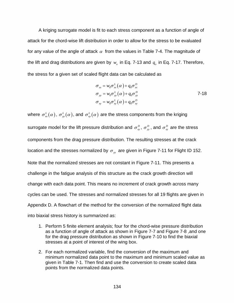
134
A kriging surrogate model is fit to each stress component as a function of angle of
attack for the chord-wise lift distribution in order to allow for the stress to be evaluated
for any value of the angle of attack from the values in Table 7-4. The magnitude of
the lift and drag distributions are given by ow in Eq. 7-13 and oq in Eq. 7-17. Therefore,
the stress for a given set of scaled flight data can be calculated as
0 0
0 0
0 0
L D
xx xx xx
L D
yy yy yy
L D
xy xy xy
w q
w q
w q
7-18
where L
xx , L
yy , and L
xy are the stress components from the kriging
surrogate model for the lift pressure distribution and D
xy , D
yy , and D
xy are the stress
components from the drag pressure distribution. The resulting stresses at the crack
location and the stresses normalized by yy are given in Figure 7-11 for Flight ID 152.
Note that the normalized stresses are not constant in Figure 7-11. This presents a
challenge in the fatigue analysis of this structure as the crack growth direction will
change with each data point. This means no increment of crack growth across many
cycles can be used. The stresses and normalized stresses for all 19 flights are given in
Appendix D. A flowchart of the method for the conversion of the normalized flight data
into biaxial stress history is summarized as:
1. Perform 5 finite element analysis; four for the chord-wise pressure distribution as a function of angle of attack as shown in Figure 7-7 and Figure 7-8 ,and one for the drag pressure distribution as shown in Figure 7-10 to find the biaxial stresses at a point of interest of the wing box.
2. For each normalized variable, find the conversion of the maximum and minimum normalized data point to the maximum and minimum scaled value as given in Table 7-1. Then find and use the conversion to create scaled data points from the normalized data points.

135
3. Create surrogate models for the lift coefficient, area under the chord-wise pressure distribution, and the biaxial stresses as a function of the angle of attack.
4. Follow Eq. 7-9 to Eq. 7-13 for the calculation of wo and Eq. 7-15 to Eq. 7-17 for the calculation of qo. This will use the surrogate models for the lift coefficient and area under the chord-wise pressure distribution.
5. Calculate the biaxial stresses from the values of wo, qo, and the surrogate models for the biaxial stresses as a function of the angle of attack.
A B Figure 7-11. The stress histories for the two-dimensional stress components for Flight
ID 152. A) Bi-axial stress components, B) Normalized stress components.
Analysis of Cracked Plate Subjected to Variable Amplitude Multi-axial Load History
Due to the fact that the stresses in this problem are non-proportional as seen in
Figure 7-11 as a function of the history (e.g. stress ratios are non-constant) this problem
creates challenges for approximating the fatigue crack growth of the problem. As the
stress history is non-proportional, the ratio of IK to IIK is non-constant, which implies
that the angle of crack growth will change as a function of the loading history. As the
path of crack growth is unknown, it is unclear how to select an analytical relationship
between the crack size and stress intensity factor which will correctly consider the
unknown crack path. Therefore, it is not possible to use a finite crack growth increment
a , as the crack growth direction cannot be assumed to be constant over a range of

136
elapsed cycles N . Therefore, the only choice is to choose the case where the cyclic
history is followed.
Before the fatigue analysis can be started, first the biaxial stresses for each of the
19 flights must be converted into equivalent cyclic stresses. This is done according to
the method outlined in Chapter 4 where an equivalent stress is calculated from the
biaxial stress components. The rainflow counting algorithm is used to find the cycles
from the equivalent stress history. The identified stress history is then superimposed
back onto the biaxial stress data, resulting in cyclic biaxial stresses which can be
applied to a plate and be used with a fatigue crack growth model. An example of the
equivalent stress for Flight ID 152 and the identified equivalent cyclic loading history is
shown in Figure 7-12. The results of the conversion from normalized data points to
stress cycles for each of the 19 flights is given in Table 7-5.
There is an uneven number of data points can be explained as the rainflow
counting method being interested in the extrema for the given data points. Not all data
points which were provided by the AFRL correspond to an extrema. The conversion
from biaxial stress components to an equivalent single stress can also result a
suppression of the number of extrema present in the resulting rainflow counting
algorithm. Two function evaluations are required for each identified cycle as the ratio of
the biaxial stresses changes between the maximum and minimum data point for each
cycle, and the calculation of the mixed-mode stress intensity factors without two function
evaluations is not possible with sufficient accuracy.
The initial geometry was that of an edge crack of initial crack size of 5 mm in a
square finite plate with sides of length 0.1 m as shown in Figure 7-13. Note that a

137
geometry with does not necessarily agree with that of an actual wingbox panel at the
specified location is used here for demonstration purposes.. The material was assumed
to be aluminum 7075-T6 where the material properties and model constants are:
Young’s modulus of 70 GPa, Poisson’s ratio of 0.3, yield stress of 520 MPa, Mode I
threshold stress intensity factor of 2.2 MPa m , Mode II threshold stress intensity factor
of 1.0 MPa m , Paris model constant of 6.85·10-11, Paris model exponent of 3.21,
shaping parameters n , , and 1 of 0.30, 0.70, and 0.84 respectively [27, 133]. To
encourage consistent, small scale crack growth the stresses calculated from the
analysis of the wing box were scaled linearly by a factor of 10, which resulted in crack
growth between 10-9 and 10-5 cycles for most of the cycles. In order to make the solution
of this problem more affordable, the proposed exact reanalysis algorithm of Chapter 6 is
used for the 74,014 required function evaluations.
A B
Figure 7-12. Equivalent stress and identified cycles from equivalent stress for Flight ID 152. A) Equivalent stress, B) Identified cycles.
A study was performed on the initial edge crack geometry to ensure that the
mixed-mode stress intensity factors converged according the mesh density. This mesh
was found to be that of a structured mesh of square elements with sides of length 1/200
m. The average computer time for each function evaluation was approximately 2.3

138
seconds with the proposed exact reanalysis algorithm, which corresponds to about 2
days for a single analysis. As the computational cost without reanalysis is too high for a
complete analysis, 100 iterations without the reanalysis algorithm were performed such
that an estimate of the total computer time without the reanalysis algorithm could be
approximated for the purposes of comparison. It was found that the mean computer
time for a cycle for these 100 iterations without reanalysis was about 20 seconds, which
would correspond to about 17 days for a proposed fatigue analysis. Note that as crack
growth occurs and more degrees of freedom are added to the system of equations, the
cost of assembly, factorization, and solving will increase. Due to this, it is very possible
that the true computer time required would be in excess of the predicted time of 17
days.
Table 7-5. Summary of the AFRL data, the number of cycles identified, and the number of function evaluations for each Flight ID.
Flight ID Number of Data Point Number of Identified Cycles Function Evaluations
2 11,158 1,780 3,560 8 12,893 2,207 4,414 10 6,050 1,409 2,818 12 9,628 1,838 3,676 16 7,544 1,311 2,622 18 7,422 1,126 2,252 22 4,057 797 1,594 26 10,124 1,895 3,790 138 6,038 1,270 2,540 140 10,427 2,275 4,550 146 10,431 2,266 4,532 148 9,766 2,290 4,580 150 16,038 3,415 6,830 152 15,120 3,470 6,940 154 11,044 2,754 5,508 156 5,631 1,025 2,050 159 7,616 1,669 3,338 161 9,623 2,180 4,360 163 9,978 2,030 4,060 Total 180,588 37,007 74,014

139
Figure 7-13. The boundary conditions and applied bi-axial stresses for the analysis of a
panel on an airplane wing box subjected to variable amplitude fatigue.
The initial and final crack paths from the analysis are given in Figure 7-14. For a
more detailed view of the crack propagation path, refer to Figure 7-15. Note that initially,
the crack tip begins to move down and to the right. This agrees with the observation that
the largest stress component is yy , followed by xy . With the loading specified in
Figure 7-13, the resultant stress would be approximately perpendicular to the initial
direction of crack growth. For the initial crack xx has no effect on either the stress
intensity factors or the crack propagation path. The subsequent crack propagation path
represents a more difficult challenge to analyze in detail as the changing orientation of
the crack tip represents a changing crack tip coordinate system and resultant stress
acting at the crack tip in the Mode I and II. The general trend is to move in a horizontal
motion, which is consistent with yy being the largest applied stress.
The crack length as a function of the cycle number is given in Figure 7-16 where
the grey lines denote the bounds associated with each unique flight. One of the
xx xx
yy
τxy
a
W

140
observations from these plots is that most of the crack growth occurs early in the life of
the wing panel. In fact, of the 37,007 loading cycles, crack growth occurs in only about
2,500 of these cycles. This can be explained partially with the assistance of Figure 7-17,
which gives the Mode I and II stress intensity factor ranges as a function of cycle
number. Recall, that the threshold Mode I and II stress intensity factor ranges for
aluminum were identified as taking values of 2.2 MPa m and 1.0 MPa m . From
Figure 7-17 it is clear that rarely does the Mode I stress intensity factor range exceed
this value. Furthermore, it can be noticed that early in the panel’s life, the Mode I stress
intensity factor range tends to take larger values than later in the panels life. Later in the
lift of the panel, when the Mode II stress intensity range takes larger values, the Mode I
values are at a minimum, reducing the net effect of increased IIK . It should also be
recalled that the predicted stresses at the crack location were increased by a factor of
10 to encourage an increased amount of crack growth throughout the panel’s life. In a
real application it is unlikely that this level of crack growth would occur at such an
accelerated rate.
A B
Figure 7-14. The initial and final crack geometries from the stresses identified through the normalized flight data from the AFRL. A) Initial crack, B) final crack

141
Figure 7-15. Close-up view of the final crack geometry from the stresses identified
through the normalized flight data from the AFRL.
Figure 7-16. Comparison of the crack length as a function of the cycle number for the
19 flights from the normalized AFRL data.
Another cause for the reduced amount of crack growth later in the panels life may
be considered as a function of the RM and PM terms in the modified Paris model used
in the analysis. The stress ratio R will increase the value of RM , and therefore,
accelerate crack growth. It can easily be seen in Figure 7-17 that the value of R will be

142
take a maximum value early in the life of the panel. An observation about what may be
perceived as jumps in the crack length around cycle numbers 3500, 4000, 6000, and
9000. Each of these instances has a corresponding peak in the IK curve. This peak
will act as an overload, increasing the plasticity at the crack tip and slowing crack
growth until the point in time when a load is applied which results in the creation of a
larger plastic zone. As most of the peaks in the IK curve exist early in the life of the
panel, the crack growth later in the panel's life is retarded as there are few instances
where the applied load to exceed the previously developed crack tip plasticity.
A B Figure 7-17. The Mode I and Mode II stress intensity factor ranges for the 37,007
cycles. A) Mode I stress intensity factor range, B) Mode II stress intensity factor range.
Summary
The fatigue analysis of an airplane wing subjected to mixed-mode variable
amplitude loading was conducted through the use of a simple stress model of an
airplane wing box in coordination with normalized flight data provided by the AFRL.
First, the normalized flight data was scaled to approximate values related to a
commercial aircraft flight and a Boeing 767 in particular. Then, the two-dimensional
stress history from the 180,588 normalized data points was calculated at a particular

143
point of interest along an airplane wing. Next, an equivalent stress was calculated and
the rainflow counting algorithm was used in order to convert the stress data into cyclic
loading data consisting of 37,007 cycles which could be used in a fatigue crack growth
model. These cycles were then superimposed onto the xx , yy, and xy
stress
histories.
Due to the non-proportional loading represented by the stress histories, fatigue
modeling techniques which assume multiple elapsed cycles for each simulation cannot
be used to solve this problem. Instead, each loading cycle was modeled using the exact
XFEM reanalysis method based upon the direct modification of an existing Cholesky
factorization. It was estimated that the combination of savings in assembly and
factorization time for this problem resulted in the problem being solved in about 86% of
the time that would be needed for the traditional solution procedure. At each cycle, the
crack growth direction was calculated according to the maximum circumferential stress
criterion. The fatigue crack growth model which was used was a modified version of the
classical Paris model which also considers the effects of the threshold stress intensity
factor, stress ratio R, and load interactions as a function of the changes in plasticity as a
result of overloads and underloads. The mixed-mode stress intensity factors are
converted into a single equivalent stress intensity factor for use in the modified Paris
model through the use of the methods introduced by Liu.
Over the life of the panel, crack growth occurred in about 2,500 of the 37,000
modeled cycles. However, this is not information which would have been available
before the analysis was run as no information about the amount or direction of crack
growth was known before modeling the response of the panel to the biaxial stresses.

144
Crack growth in a limited number of cycles was caused by a combination of the stress
intensity factor ranges rarely exceeding the threshold values and the crack tip plasticity
model in the modified Paris model which retarded crack growth. It was observed that
the stress intensity factor history for the crack showed that early in the panel's life,
greater maximum values of IK and IIK were often realized. This resulted in an
increased amount of crack growth early in the life of the panel. Later in the panels life,
crack growth occurred more slowly and in a more controlled fashion, most likely due to
both the lower peak values of the stress intensity factor ranges as well as the crack tip
plasticity which had been developed earlier in the panels life.

145
CHAPTER 8 CONCLUSIONS AND FUTURE WORK
Conclusions
Fatigue is the process by which materials fail due to repeated loading well below
the levels that they would fail under static loading conditions. It is not uncommon for 104
to 108 cycles to be needed for failure to occur. This presents a challenge for
computational simulation as this number of cycles is not feasible for modeling in a finite
element environment. With classical finite element methods, the mesh corresponds to
the domain of interest, which means that the mesh must be recreated locally around the
crack tip each time crack growth occurs. Fatigue crack growth has been one of the
leading causes of aircraft accidents throughout history and still causes incidents today.
Better computational tools for the modeling of fatigue crack growth will help to reduce
the risk of accidents from the initiation and propagation of a crack. The goal of this work
is to create strategies such that fatigue crack growth can be numerically modeled with
greatly reduced computational requirements.
The challenges associated with mesh generation in the classical finite element
method are addressed through the use of the extended finite element method (XFEM).
In the XFEM, discontinuities are represented independent of the finite element mesh.
Even when the challenges associated with mesh generation can be avoided; there is
still a large number of function evaluations required in modeling fatigue crack growth.
The fundamental structure of XFEM can be exploited to further reduce the cost of the
repeated function evaluations necessary for modeling fatigue crack growth. When crack
growth occurs in the XFEM, only a small portion of the finite element stiffness matrix
changes as crack growth occurs. These small changes in the finite element stiffness

146
matrix are exploited through the direct modification of an existing Cholesky factorization
through the use of row add and row delete operations. The approximate fill-reducing
ordering for this matrix which has changing, but unknown connectivity is found through
the use of a dummy stiffness matrix.
Surrogate models enable the use of higher-order numerical methods in the
integration of a fatigue crack growth model for both the magnitude and direction of crack
growth with the use of a single expensive finite element simulation. Test cases show
that the use of kriging to replace expensive function evaluations offers comparable
accuracy to classical numerical techniques with significantly fewer expensive function
evaluations. A variable integration step size algorithm is also introduced which uses the
difference between the surrogate prediction and the finite element simulations to
dynamically change the integration step size to attempt to achieve some target
accuracy for each simulation. In the case that the particular iteration has accuracy less
than the target error, then the integration step size is increased. Similarly, for an
iteration where the accuracy is greater than the target error, the integration step size is
decreased.
Finally, the XFEM exact reanalysis algorithm is used to predict fatigue crack
growth due to variable amplitude biaxial loading in an airplane wing box. Normalized
data from the Air Force research laboratory was scaled and then used to create a stress
history for the airplane wing in terms of the scaled data. The rainflow counting algorithm
was used to convert the discrete stress history into a cyclic stress history which was
used as the input for the fatigue analysis. This is a first step towards realizing fatigue

147
crack growth from service load histories for variable amplitude multi-axial stress
histories.
Future Work
Future Development of MXFEM
Additional enrichment functions could be implemented for cracks or inclusions,
giving the user more options for learning about the XFEM, of particular interest may be
allowing only the Heaviside enrichment for a crack and neglecting the crack tip terms,
as this comparison is often made in the literature. Contact between crack faces could be
implemented to prevent for the crack surfaces from entering the materials as would
currently occur for compressive loading. Modifying the definition of where boundary
conditions and loading are applied instead of requiring the direct modification of files
other than the input file for the given loading conditions may facilitate the ease of use for
simulations. Removing the limitation for square elements and a rectangular domain,
perhaps with the option to import the nodal coordinates and element connectivity
information from a text file which would allow for complex geometries to be considered.
Possible Application for the Exact XFEM Reanalysis Algorithm
An example of a crack growth problem which could benefit from an application of
the proposed exact XFEM reanalysis algorithm is that of elastic crack growth between
dissimilar materials. Consider the case of a crack which is propagating towards a
material interface as shown in Figure 8-1. Upon reaching the interface the crack may
either be arrested, penetrate into the interface, propagate along the interface or branch
and propagate along the interface [209]. The challenge in modeling this problem is that
the crack propagation behavior is a function of the two materials which are considered
as well as the angle at which the crack approaches the interface. There is no closed

148
form solution for how the crack will behave upon reaching the interface, and one
possible solution procedure would involve the solution of an optimization problem to find
the path with the greatest energy release rate from the available possible propagation
paths.
Figure 8-1. Possible crack propagation paths between dissimilar materials. A) Arrest,
B) Penetration, C) Propagate along interface, D) Branch along interface.
The proposed exact XFEM reanalysis algorithm could be used to create an
optimization problem where the penetration or growth patterns along the material
interface are considered. The angle of penetration which maximizes the energy release
rate could be compared to the energy release rates for growth along the interface or
crack branching at the interface with the maximum energy release rate among these
options being the most likely crack growth path. This energy release rate can then be
converted to a stress intensity value and compared with the fracture toughness of the
A
C
B
D
Material 1 Material 2 Material 1 Material 2
Material 1 Material 2 Material 1 Material 2

149
material interface or material into which the crack is penetrating. If the stress intensity is
not sufficiently large to cause fracture, then the case of a crack arresting at the interface
may be observed. The major modifications which need to be considered for this
problem with the MXFEM code include: implementation and verification of bi-material
[85] and branching [89] crack enrichment functions, the implementation of the auxiliary
stress and displacement states for the bi-material crack [85], and the formulation of the
optimization problem to determine the direction of maximum energy release rate. The
analysis may be verified against the work of He [209, 210] and Zhang [211]. If this
implementation was completed it would be possible to further expend this approach to
interface layers [212] and laminates [213].
Possible Applications for Surrogate Integration
An example of a problem which may benefit from the use of the proposed
surrogate integration method is that of wear occurring in the joint of multibody systems
due to contact. The Archard wear model [214] is commonly used to predict the amount
of wear such that
d
d
hkp s
s 8-1
where h is the wear depth, k is a wear constant, p is the contact pressure between the
two bodies in contact, and s is the sliding distance between the two bodies. Note that
this problem is quite similar in form to the classical Paris model where a correlation
could be made where C k , K p s , and 1m . Finite element simulations with a
contact model are commonly used to calculate the contact pressure and sliding distance
[215], while the wear constant k usually is determined from experimental data.

150
Wear is a slow process which occurs over a large number of iterations, similar to
fatigue. In this way, it would be too expensive to perform a finite element simulation
during each loading cycle to find p and s, calculate the wear depth, update the mesh,
and then perform the next analysis. Instead, a forward Euler approach [215] is often
used to approximate the wear over a number of elapsed cycles N according to a
single finite element simulation for p and s as
h kp s N . 8-2
This is the same basic problem which was considered in the case of modeling fatigue
crack growth and it is possible that the use of kriging extrapolation and/or the variable
step size approach could be applied to a wear analysis and result in a better
approximation of the amount of total wear h over a number of elapsed cycles N with
some modifications to account for the differences between the two problems.

151
APPENDIX A MXFEM BENCHMARK PROBLEMS
XFEM Enrichments
Center Crack in a Finite Plate
The first problem considered in the verification of the MATLAB® XFEM code is that
of a center crack in a finite plate. The geometry and specifications for the values of a
and W is shown in Figure A-1. The material properties used in the analysis were
chosen to be Young’s modulus of 10 MPa and Poisson’s ratio of 0.3. The full domain
was a plate with height 10 m and width 6 m with a center crack of length 2 m. The
applied stress was 1 Pa. Square plane strain quadrilateral elements with a structured
mesh were used. Both a full and half model were considered based on the symmetry in
the problem.
The theoretical stress intensity factor for a center crack in a finite plate [20] is
2 43
sec 12 40 50
t
IK a A-1
where a W , is the applied stress, and a is the half crack length. A comparison of
the convergence as a function of the average element size h is given in Table A-1
where the normalized stress intensity factors are given as
XFEM
n II t
I
KK
K A-2
where t
IK is given by Eq. A-1 and XFEM
IK is the value calculated by the XFEM analysis
using the domain form of the contour integral. The results for the analysis of the full and
half model are given in Table A-1. From this table it can be noticed that an accurate
solution is achieved for a mesh with characteristic element size of 1/20. There is limited

152
improvement with increased mesh density in the vicinity of the crack tip. It can be
noticed that there is a difference between the full and half model created by symmetry.
These changes are most likely due to the slightly different boundary conditions used for
the two cases. In the case of a full center crack, the midplane where the crack is located
is restricted from moving the vertical direction and the midpoint of the plate is fixed. For
the half model, the left edge are given rollers in the y-direction and the bottom left hand
corner is fixed. The XFEM model shows good accuracy without any of the cumbersome
challenges associated with solving a similar problem in the traditional FEM framework.
Figure A-1. Representative geometry for a center crack in a finite plate.
Table A-1. Convergence of normalized stress intensity factors for a full and half model for a center crack in a finite plate.
h n
IK Full, Right Tip n
IK Full, Left Tip n
IK Half, Right Tip
1/5 0.954 0.952 0.962 1/10 0.977 0.977 0.967 1/20 0.989 0.989 0.980 1/40 0.996 0.996 0.990 1/80 0.999 0.999 0.996
2a
2W

153
Edge Crack in a Finite Plate
The next problem considered in the verification of the MATLAB® XFEM code is
that of an edge crack in a finite plate. The geometry and specifications for the values of
a and W is shown in Figure A-2. The material properties used in the analysis were
chosen to be Young’s modulus of 10 MPa and Poisson’s ratio of 0.3. The full domain
was a plate with height 6 m and width 3 m with a center crack of length 1 m. The
applied stress was 1 Pa. Square plane strain quadrilateral elements with a structured
mesh were used.
Figure A-2. Representative geometry for an edge crack in a finite plate
The theoretical stress intensity factor for an edge crack in a finite plate [20] is
2 3 41.12 0.231 10.55 21.72 30.39 t
IK a A-3
where a W , is the applied stress, and a is the characteristic crack length. A
comparison of the convergence as a function of the average element size h is given in
Table A-2 where the normalized stress intensity factors are given by Eq. A-2. From this
H
W
a

154
table it can be noticed that an accurate solution is achieved for a mesh with
characteristic element size of 1/10. There is limited improvement with increased mesh
density in the vicinity of the crack tip. This represents a decreased mesh density to be
needed for a solution of comparable accuracy to the case of a center crack in a finite
plate. This can be explained by the value of the Mode I stress intensity factor in this
case taking a larger value than in the previous example, which makes the normalization
less sensitive to small differences between the theoretical and calculated values.
Table A-2. Convergence of normalized stress intensity factors for an edge crack in a finite plate.
h n
IK
1/5 0.884 1/10 0.991 1/20 1.001 1/40 1.002 1/80 1.002
Inclined Edge Crack in a Finite Plate
The case of an inclined edge crack in a finite plate benchmark problem is used to
show accuracy in mixed-mode problems. A figure of the geometry is given in Figure A-
3. The material properties used in the analysis were chosen to be Young’s modulus of
10 MPa and Poisson’s ratio of 0.3. The full domain was a plate with height 2 m and
width 1 m with an edge crack from (0,1) to (0.4,1.4). The applied stress was 1 Pa.
Square plane strain quadrilateral elements with a structured mesh were used.
A comparison of the convergence as a function of the average element size h is
given in Figure A-3 where the normalized stress intensity factors are given by Eq. A-2.
The reference solution [216] which was used for comparison is t
IK = 1.927 and t
IIK =
0.819. This reference solution is commonly used in the XFEM literature [96] and is a
solution with accepted accuracy. convergence of the Mode I and Mode II stress intensity

155
factors for this problem are comparable to that for the center crack in a finite plate
problem.
Figure A-3. Representative geometry for an inclined edge crack in a finite plate.
Table A-3. Convergence of normalized stress intensity factors for an inclined edge crack in a finite plate.
h n
IK n
IIK
1/10 0.958 1.028
1/20 0.980 1.022
1/40 0.987 1.018
1/80 0.990 1.016
Hard Inclusion in a Finite Plate
The inclusion enrichment shown in Figure A-4 is calibrated based on results from
the commercial finite element code Abaqus®. The material properties used in the
analysis were chosen to be Young’s modulus of 50 GPa and Poisson’s ratio of 0.3 for
the plate and Young’s modulus of 70 GPa and Poisson’s ratio of 0.3 for the inclusion.
The full domain was a plate with height 10 m and width 6 m with a center inclusion of
W
a
H

156
radius 0.5 m. Through symmetry only the top right hand quarter of the plate was
modeled. The applied stress was 1 Pa. Square plane strain quadrilateral elements with
a structured mesh with average element size h of 1/30 m were used for comparison
against Abaqus®.
The stress contours for the Abaqus® and MXFEM solutions are presented in
Figure A-5 ,Figure A-6 , and Figure A-7. All contours have color bars with matching
ranges. Abaqus® plots from black to grey, while MATLAB® plots from black to white,
which results is some slight differences between figures. Note that there is also a
difference in how the interface is represented as Abaqus® plots a black line, while the
MXFEM code denotes all inclusions with a white line. Some of the differences in contour
shape may be attributed to a different number of contours being plotted in the two
programs.
Figure A-4. Representative geometry for a hard inclusion in a finite plate.
2H
2W
r

157
A B
Figure A-5. The xx contours for a hard inclusion. A) Abaqus®, B) MXFEM.
A B
Figure A-6. The xy contours for a hard inclusion. A) Abaqus®, B) MXFEM.
A B
Figure A-7. The yy contours for a hard inclusion. A) Abaqus®, B) MXFEM.

158
Void in an Infinite Plate
The void enrichment function is verified against the Abaqus® solution for the
traditional FEM solution of a plate containing a hole. The material properties used in the
analysis were chosen to be Young’s modulus of 10 MPa and Poisson’s ratio of 0.3. The
full domain was a plate with height 3 m and width 3 m with a center hole of radius 0.3 m.
The applied stress was 1 Pa. Square plane strain quadrilateral elements with a
structured mesh with average element size h of 1/20 m was used.
The stress contours based on the Abaqus® solution are compared to the XFEM
stress contours in Figure A-9, Figure A-10, and Figure A-11. All stress components
show excellent agreement with the Abaqus® values. Any differences can be attributed to
either having a structured mesh for the XFEM solution compared to a conforming mesh
for the Abaqus® solution or the color scale in Abaqus® going from black to grey, while it
goes from black to white within MATLAB®.
Figure A-8. Representative geometry for a void in an infinite plate.
H
W
r

159
A B
Figure A-9. The xx contours for a void in an infinite plate. A) Theoretical, B) MXFEM.
A B
Figure A-10. The xy contours for a void in an infinite plate. A) Abaqus®, B) MXFEM.
A B
Figure A-11. The yy contours for a void in an infinite plate. A) Abaqus®, B) MXFEM.

160
Other Benchmarks
Angle of Crack Initiation from Optimization
An optimization algorithm is introduced using fminbnd in MATLAB® to determine
the angle of crack initiation which results in the maximum energy release rate. The
example of a 8 m x 8 m plate with a hole with 1 m radius subjected to uniaxial tension
as shown in Figure A-12 is used to show that the optimization implementation has been
completed with accuracy. Square plane strain quadrilateral elements with a structured
mesh with an average element size of h equal to 1/20 m was used. For this problem the
location of maximum stress corresponds to the angle of crack initiation for a 0.15 m
crack which will result in the maximum energy release rate. For a plate under uniaxial
tension this angle is 0 or radians.
Figure A-12. Representative geometry for a crack initiating at an angle θ for a plate with
a hole.
The optimization problem used to benchmark the implementation of the XFEM
optimization subroutine is given as
H
W
ai
θ

161
2 2
min
s.t .
I II
eff eff
L U
K KG
E E A-4
where G is the energy release rate, IK and
IIK are the Mode I and II stress intensity
factors, L and U are the lower and upper bounds on the angle and
effE is given as
2
plane stress
plane strain1
eff
E
E E . A-5
The results are presented in Table A-4 for two sets of bounds - 2 ≤ ≤ 2 and
2 ≤ ≤ 3 2 . Results are presented as the optimum angle identified opt by fminbnd
with the function tolerance set to 1E-9 and the angle tolerance set to 1E-6. The
normalized energy release rate is
XFEM
n
t
GG
G A-6
where tG is the energy release rate corresponding to an initiation angle of 0 or
radians and XFEMG is the energy release rate from the optimization with the XFEM. For
this example the theoretical maximum energy release rate is given as tG = 3.5166E-7
J/m2. Based upon the function and angle tolerances, the solutions represent an
excellent agreement between the known solution and the MXFEM optimization result.
Table A-4. Comparison of the theoretical and MXFEM value for maximum energy release angle as a function of average element size.
- 2 ≤ ≤ 2 2 ≤ ≤ 3 2
h opt nG opt nG
1/20 -1.715E-5 1.001 3.142 1.000

162
Crack Growth in Presence of an Inclusion
Bordas [69] presented the case of edge crack growth under mixed-mode loading
in a plate with either a hard or soft inclusion. This problem acts to verify the
implementation of mixed-mode crack problems, the inclusion enrichment function, and
the use of both the crack and inclusion enrichment functions in a single framework. The
material properties used in the analysis were chosen to be Young’s modulus of 1 GPa
and Poisson’s ratio of 0.3 for material 1 and Young’s modulus of 10 GPa and Poisson’s
ratio of 0.3 for material 2. For the case of a hard inclusion, material 2 is for the inclusion
and material 1 is for the plate. For the case of a soft inclusion, material 1 is for the
inclusion and material 2 is for the plate. The full domain was a plate with height 8 m and
width 4 m with an edge crack of length 0.5 m centered on the left edge. The circular
inclusion of radius 1 is placed at the horizontal midpoint and the vertical quarter point.
There were 34 iterations of growth where at each iteration the amount of growth
was equal to a = 0.1 m and in the direction given by the maximum circumferential
stress predicted by a unit tensile load which was applied to the top edge of the domain
in the y-direction. Square plain strain quadrilateral elements with a structured mesh with
average element size h of 1/20 m were used. It is important to note that no boundary
conditions were given by Bordas so here it is assumed that edge crack boundary
conditions are to be used. This may explain the slight differences between the results of
Bordas and those presented in Figure A-13. Note that the scales of the x and y axis are
different, which result in the circular soft inclusion appearing to take a shape more
similar to that of an ellipse. Also, what appears to be a large initial crack growth
increment corresponds to the two data points corresponding to the initial crack
geometry.

163
A B Figure A-13. Comparison of crack paths to those predicted by Bordas for a hard and
soft inclusion. A) Hard inclusion, B) Soft inclusion.
Fatigue Crack Growth
The implementation of the Paris model [34] for fatigue crack growth was verified
within the XFEM framework. The Paris model predicts that crack growth occurs
according to the differential equation
d
d
maC K
N A-7
where d da N is the crack growth rate, C is the Paris model constant, m is the Paris
model exponent, and K is the stress intensity factor range under cyclic loading. Here
the geometry is chosen to mimic a center crack in an infinite plate where K is
K a A-8
where is the applied stress range and a is the half crack length.
The material properties used in the analysis were chosen to be Young’s modulus
of 71.7 GPa, Poisson’s ratio of 0.33, Paris model constant of 1.5E-10, and Paris model
exponent of 3.8. The full domain was a plate with height 0.4 m and width 0.6 m with a
center crack of length 0.02 m. The applied stress was 78.6 MPa. Square plane strain
quadrilateral elements with a structured mesh with average element size h of 1/500 m

164
was used. Through symmetry, only the right half of the geometry was modeled. Fatigue
crack growth was measure to 2450 cycles with step sizes of N equal to 50 at each
simulation. A comparison of the theoretical and simulated crack growth is given in
Figure A-14. From this analysis it is apparent that the XFEM and Paris model solutions
are in good agreement. As the crack size increases, there begins to be a difference
between the two solutions. It is likely that the choice of a smaller number of elapsed
cycles at each iteration would reduce the differences between the two predictions for
large crack sizes.
Figure A-14. Comparison between Paris model and XFEM simulation for fatigue crack
growth for a center crack in an infinite plate.

165
APPENDIX B AUXILIARY DISPLACEMENT AND STRESS STATES
The auxiliary displacement and stress states given by Westergaard [145] and
Williams [146] for that are used in the interaction integrals [16, 18, 19] to calculate the
stress intensity factors are given in terms of polar coordinates from crack tip r and ,
shear modulus , Poisson's ratio , and Kosolov constant as
1
1cos cos sin 2 cos
2 2 2 2
I II
ru K K 10-1
2
1sin sin cos 2 cos
2 2 2 2
I II
ru K K 10-2
3
2sin
2 2
III
ru K 10-3
11
1 3 3cos 1 sin sin sin 2 cos cos
2 2 2 2 2 22
I IIK K
r 10-4
22
1 3 3cos 1 sin sin sin cos cos
2 2 2 2 2 22
I IIK K
r 10-5
33 11 22 10-6
23
1cos
22
IIIK
r 10-7
31
1sin
22
r 10-8
12
1 3 3sin cos cos cos 1 sin sin
2 2 2 2 2 22
I IIK K
r 10-9
3plane stress
1
3 4 plane strain
. 10-10

166
APPENDIX C CONVERSION OF NORMALIZED FLIGHT DATA TO SCALED FLIGHT DATA
Table C-1. Normalized and scaled flight data with conversion for Flight ID 2.
Variable Norm Min Norm Max Scaled Min Scaled Max Conversion
g 0.0186 0.908 0.75 1.5 g = 0.843gnorm+0.734 θB -0.711 0.574 0 30 θB = 23.2aroll+16.5 mfuel 0.00 0.971 800 50,000 mfuel = 51500fnorm M 0.0191 0.921 0 0.80 M = 0.887Mnorm-0.0170 v 0.0222 0.822 0 236 v = 295vnorm-6.56 α 0.0178 0.853 0.001 10 α = 12.0αnorm-0.212
Table C-2. Normalized and scaled flight data with conversion for Flight ID 8.
Variable Norm Min Norm Max Scaled Min Scaled Max Conversion
g -0.0609 0.914 0.75 1.5 g = 0.769gnorm+0.797 θB -0.485 0.490 0 30 θB = 30.8aroll+14.9 mfuel 0.00 0.990 800 50,000 mfuel = 50500fnorm M 0.0191 0.954 0 0.80 M = 0.856Mnorm-0.0163
v 0.0222 0.962 0 236 v = 252vnorm-5.59 α 0.00 0.833 0.001 10 α = 12.0αnorm+0.001
Table C-3. Normalized and scaled flight data with conversion for Flight ID 10.
Variable Norm Min Norm Max Scaled Min Scaled Max Conversion g 0.0793 0.337 0.75 1.5 g = 2.91gnorm+0.519 θB -0.196 0.195 0 30 θB = 76.7aroll+15.0 mfuel 0.00 0.986 800 50,000 mfuel = 50700fnorm M 0.191 0.579 0 0.80 M = 1.43Mnorm-0.0273 v 0.0222 0.663 0 236 v = 369vnorm-8.19 α 0.00 0.844 0.001 10 α = 11.9αnorm+0.001
Table C-4. Normalized and scaled flight data with conversion for Flight ID 12.
Variable Norm Min Norm Max Scaled Min Scaled Max Conversion g 0.0599 0.847 0.75 1.5 g = 0.952gnorm+0.693 θB -0.324 0.312 0 30 θB = 47.2aroll+15.3 mfuel 0.00 0.993 800 50,000 mfuel = 50400fnorm M 0.0191 0.867 0 0.80 M = 0.944Mnorm-0.0180 v 0.0222 0.828 0 236 v = 293vnorm-6.51 α 0.00 0.723 0.001 10 α = 13.8αnorm+0.001
Table C-5. Normalized and scaled flight data with conversion for Flight ID 16.
Variable Norm Min Norm Max Scaled Min Scaled Max Conversion
g 0.0248 0.965 0.75 1.5 g = 0.797gnorm+0.730 θB -0.639 0.634 0 30 θB = 31.2aroll+19.9 mfuel 0.00 0.996 800 50,000 mfuel = 50200fnorm M 0.0191 0.987 0 0.80 M = 0.827Mnorm-0.0158 v 0.0222 0.919 0 236 v = 264vnorm-5.85 α 0.00 0.794 0.001 10 α = 12.6αnorm+0.001

167
Table C-6. Normalized and scaled flight data with conversion for Flight ID 18.
Variable Norm Min Norm Max Scaled Min Scaled Max Conversion
g -0.145 0.880 0.75 1.5 g = 0.732gnorm+0.856 θB -0.817 0.759 0 30 θB = 19.0aroll+15.5 mfuel 0.00 0.941 800 50,000 mfuel = 53100fnorm M 0.0191 0.941 0 0.80 M = 0.868Mnorm-0.0166 v 0.0222 0.825 0 236 v = 295vnorm-6.54 α 0.00 0.721 0.001 10 α = 13.9αnorm+0.001
Table C-7. Normalized and scaled flight data with conversion for Flight ID 22.
Variable Norm Min Norm Max Scaled Min Scaled Max Conversion g 0.0838 0.848 0.75 1.5 g = 0.981gnorm+0.668 θB -0.488 0.505 0 30 θB = 30.2aroll+14.7 mfuel 0.00 0.998 800 50,000 mfuel = 50100fnorm M 0.0191 0.947 0 0.80 M = 0.862Mnorm-0.0165 v 0.0222 0.821 0 236 v = 296vnorm-6.57 α 0.00 0.819 0.001 10 α = 12.2αnorm+0.001
Table C-8. Normalized and scaled flight data with conversion for Flight ID 26.
Variable Norm Min Norm Max Scaled Min Scaled Max Conversion g 6.88E-4 0.586 0.75 1.5 g = 1.28gnorm+0.749 θB -0.463 0.291 0 30 θB = 39.8aroll+18.4 mfuel 0.00 0.992 800 50,000 mfuel = 50400fnorm M 0.0191 0.617 0 0.80 M = 1.34Mnorm-0.0256 v 0.0222 0.709 0 236 v = 344vnorm-7.65 α 0.0178 0.858 0.001 10 α = 11.9αnorm+0.001
Table C-9. Normalized and scaled flight data with conversion for Flight ID 138.
Variable Norm Min Norm Max Scaled Min Scaled Max Conversion g -0.0269 0.882 0.75 1.5 g = 0.825gnorm+0.772 θB -0.569 0.651 0 30 θB = 24.6aroll+14.0 mfuel 0.00 0.913 800 50,000 mfuel = 54700fnorm M 0.0191 0.961 0 0.80 M = 0.849Mnorm-0.0162 v 0.0222 0.836 0 236 v = 290vnorm-6.45 α 0.00890 0.869 0.001 10 α = 11.6αnorm+0.001
Table C-10. Normalized and scaled flight data with conversion for Flight ID 140.
Variable Norm Min Norm Max Scaled Min Scaled Max Conversion g 0.00730 1.00 0.75 1.5 g = 0.756gnorm+0.744 θB -0.607 0.756 0 30 θB = 22.0aroll+13.4 mfuel 0.00 0.934 800 50,000 mfuel = 53500fnorm M 0.0191 0.951 0 0.80 M = 0.886Mnorm-0.0163 v 0.0222 0.838 0 236 v = 290vnorm-6.43 α 0.0124 0.799 0.001 10 α = 12.7αnorm-0.157

168
Table C-11. Normalized and scaled flight data with conversion for Flight ID 146.
Variable Norm Min Norm Max Scaled Min Scaled Max Conversion
g -0.0775 0.913 0.75 1.5 g = 0.757gnorm+0.809 θB -0.709 0.727 0 30 θB = 20.9aroll+14.8 mfuel 0.00 0.914 800 50,000 mfuel = 54700fnorm M 0.0190 0.991 0 0.80 M = 0.823Mnorm-0.0156 v 0.0222 1.00 0 236 v = 242vnorm-5.37 α 0.00 0.879 0.001 10 α = 11.3αnorm+0.001
Table C-12. Normalized and scaled flight data with conversion for Flight ID 148.
Variable Norm Min Norm Max Scaled Min Scaled Max Conversion g -0.0136 0.954 0.75 1.5 g = 0.775gnorm+0.761 θB -0.775 0.611 0 30 θB = 21.6aroll+16.8 mfuel 0.00 0.961 800 50,000 mfuel = 52000fnorm M 0.019 1.00 0 0.80 M = 0.815Mnorm-0.0155 v 0.0222 0.983 0 236 v = 246vnorm-5.46 α 0.00 0.908 0.001 10 α = 11.0αnorm+0.001
Table C-13. Normalized and scaled flight data with conversion for Flight ID 150.
Variable Norm Min Norm Max Scaled Min Scaled Max Conversion g -0.169 0.919 0.75 1.5 g = 0.689gnorm+0.866 θB -0.920 0.745 0 30 θB = 18.0aroll+16.6 mfuel 0.00 0.956 800 50,000 mfuel = 52300fnorm M 0.0190 0.954 0 0.80 M = 0.856Mnorm-0.0163 v 0.0222 0.837 0 236 v = 290vnorm-6.44 α 0.00 1.00 0.001 10 α = 10.0αnorm+0.001
Table C-14. Normalized and scaled flight data with conversion for Flight ID 152.
Variable Norm Min Norm Max Scaled Min Scaled Max Conversion g -0.208 0.957 0.75 1.5 g = 0.644gnorm+0884 θB -1.00 0.624 0 30 θB = 18.5aroll+18.5 mfuel 0.00 0.975 800 50,000 mfuel = 51300fnorm M 0.0191 0.977 0 0.80 M = 0.835Mnorm-0.0159 v 0.0222 0.839 0 236 v = 289vnorm-6.42 α 0.00 0.853 0.001 10 α = 11.7αnorm+0.001
Table C-15. Normalized and scaled flight data with conversion for Flight ID 154.
Variable Norm Min Norm Max Scaled Min Scaled Max Conversion g -0.011 0.922 0.75 1.5 g = 0.804gnorm+0.759 θB -0.696 0.513 0 30 θB = 24.8aroll+17.3 mfuel 0.00 0.993 800 50,000 mfuel = 50400fnorm M 0.0191 0.979 0 0.80 M = 0.834Mnorm-0.0159 v 0.0222 0.978 0 236 v = 247vnorm-5.49 α 0.00 0.931 0.001 10 α = 10.7αnorm+0.001

169
Table C-16. Normalized and scaled flight data with conversion for Flight ID 156.
Variable Norm Min Norm Max Scaled Min Scaled Max Conversion
g -4.20E-4 0.900 0.75 1.5 g = 0.833gnorm+0.750 θB -0.652 0.697 0 30 θB = 22.2aroll+14.5 mfuel 0.00 0.927 800 50,000 mfuel = 53900fnorm M 0.0219 0.928 0 0.80 M = 0.883Mnorm-0.0193 v 0.0256 0.821 0 236 v = 297vnorm-7.61 α 0.0373 0.831 0.001 10 α = 12.6αnorm-0.469
Table C-17. Normalized and scaled flight data with conversion for Flight ID 159.
Variable Norm Min Norm Max Scaled Min Scaled Max Conversion g -0.0765 0.917 0.75 1.5 g = 0.755gnorm+0.808 θB -0.530 0.492 0 30 θB = 29.3aroll+15.6 mfuel 0.00 0.946 800 50,000 mfuel = 52800fnorm M 0.0192 0.993 0 0.80 M = 0.821Mnorm-0.0158 v 0.0225 0.985 0 236 v = 246vnorm-5.53 α 0.00 0.734 0.001 10 α = 13.6αnorm+0.001
Table C-18. Normalized and scaled flight data with conversion for Flight ID 161.
Variable Norm Min Norm Max Scaled Min Scaled Max Conversion g 0.0182 0.878 0.75 1.5 g = 0.872gnorm+0.734 θB -0.492 0.471 0 30 θB = 31.2aroll+15.3 mfuel 0.00 0.936 800 50,000 mfuel = 53400fnorm M 0.0201 0.9808 0 0.80 M = 0.832Mnorm-0.0167 v 0.0236 0.966 0 236 v = 251vnorm-5.92 α 0.00 0.826 0.001 10 α = 12.1αnorm+0.001
Table C-19. Normalized and scaled flight data with conversion for Flight ID 163.
Variable Norm Min Norm Max Scaled Min Scaled Max Conversion g 0.00360 0.900 0.75 1.5 g = 0.837gnorm+0.747 θB -0.518 0.725 0 30 θB = 24.1aroll+12.5 mfuel 0.00 0.946 800 50,000 mfuel = 52900fnorm M 0.0209 0.946 0 0.80 M = 0.865Mnorm-0.0181 v 0.0244 0.843 0 236 v = 289vnorm-7.05 α 0.00890 0.879 0.001 10 α = 11.5αnorm-0.101

170
APPENDIX D STRESS HISTORIES FOR FLIGHT DATA FROM AFRL
Figure D-1. Stress history for Flight ID 2. A) Bi-axial stress, B) Normalized stress.
Figure D-2. Stress history for Flight ID 8. A) Bi-axial stress, B) Normalized stress.
Figure D-3. Stress history for Flight ID 10. A) Bi-axial stress, B) Normalized stress.

171
Figure D-4. Stress history for Flight ID 12. A) Bi-axial stress, B) Normalized stress.
Figure D-5. Stress history for Flight ID 16. A) Bi-axial stress, B) Normalized stress.
Figure D-6. Stress history for Flight ID 18. A) Bi-axial stress, B) Normalized stress.

172
Figure D-7. Stress history for Flight ID 22. A) Bi-axial stress, B) Normalized stress.
Figure D-8. Stress history for Flight ID 26. A) Bi-axial stress, B) Normalized stress.
Figure D-9. Stress history for Flight ID 138. A) Bi-axial stress, B) Normalized stress.

173
Figure D-10. Stress history for Flight ID 140. A) Bi-axial stress, B) Normalized stress.
Figure D-11. Stress history for Flight ID 146. A) Bi-axial stress, B) Normalized stress.
Figure D-12. Stress history for Flight ID 148. A) Bi-axial stress, B) Normalized stress.

174
Figure D-13. Stress history for Flight ID 150. A) Bi-axial stress, B) Normalized stress.
Figure D-14. Stress history for Flight ID 152. A) Bi-axial stress, B) Normalized stress.
Figure D-15. Stress history for Flight ID 154. A) Bi-axial stress, B) Normalized stress.

175
Figure D-16. Stress history for Flight ID 156. A) Bi-axial stress, B) Normalized stress.
Figure D-17. Stress history for Flight ID 159. A) Bi-axial stress, B) Normalized stress.
Figure D-18. Stress history for Flight ID 161. A) Bi-axial stress, B) Normalized stress.

176
Figure D-19. Stress history for Flight ID 163. A) Bi-axial stress, B) Normalized stress.

177
LIST OF REFERENCES
1. "de Havilland Comet." Wikipedia: The Free Encyclopedia. Wikimedia Foundation, Inc. 25 Oct. 2011. Web. 25 Oct. 2011.
2. "1957 Cebu Douglas C-47 Crash." Wikipedia: The Free Encyclopedia. Wikimedia Foundation, Inc. 17 Mar. 2011. Web. 25 Oct. 2011.
3. "Los Angeles Airways Flight 417." Wikipedia: The Free Encyclopedia. Wikimedia Foundation, Inc. 8 Oct. 2011. Web. 25 Oct. 2011.
4. "Alexander L. Kielland (platform)." Wikipedia: The Free Encyclopedia. Wikimedia Foundation, Inc. 25 Aug. 2011. Web. 25 Oct. 2011.
5. "Japan Airlines Flight 123." Wikipedia: The Free Encyclopedia. Wikimedia Foundation, Inc. 22 Oct. 2011. Web. 25 Oct. 2011.
6. "Aloha Airlines Flight 243." Wikipedia: The Free Encyclopedia. Wikimedia Foundation, Inc. 3 Oct. 2011. Web. 25 Oct. 2011.
7. "United Airlines Flight 232." Wikipedia: The Free Encyclopedia. Wikimedia Foundation, Inc. 8 Oct. 2011. Web. 25 Oct. 2011.
8. "El Al Flight 1862." Wikipedia: The Free Encyclopedia. Wikimedia Foundation, Inc. 23 Sep. 2011. Web. 25 Oct. 2011.
9. "Eschede Train Disaster." Wikipedia: The Free Encyclopedia. Wikimedia Foundation, Inc. 1 Oct. 2011. Web. 25 Oct. 2011.
10. "China Airlines Flight 611." Wikipedia: The Free Encyclopedia. Wikimedia Foundation, Inc. 14 Oct. 2011. Web. 25 Oct. 2011.
11. "Chalk's Ocean Airways Flight 101." Wikipedia: The Free Encyclopedia. Wikimedia Foundation, Inc. Web.
12. ACC Public Affairs. F-15 Eagle Accident Report Released, 2008, available at http://www.af.mil/news/story.asp?storyID=123081718.
13. "Southwest Airlines Flight 2294." Wikipedia: The Free Encyclopedia. Wikimedia Foundation, Inc. 18 Apr. 2011. Web. 25 Oct. 2011.
14. Beden S, Abdullah S, Ariffin A. Review of fatigue crack propagation models in metallic components. European Journal of Scientific Research 2009; 28(3):364-397.
15. Anderson TL. Fracture Mechanics: Fundamentals and Applications. CRC Press: Boca Raton, FL, 2004.

178
16. Nikishkov GP, Atluri SN. Calculation of fracture mechanics parameters for an arbitrary three-dimensional crack by the 'equivalent domain integral method'. International Journal for Numerical Methods in Engineering 1987; 24(9):1801-1821.
17. Rice JR. A path independent integral and the approximate analysis of strain concentration by notches and cracks. Journal of Applied Mechanics 1968; 35(2):379-386.
18. Shih C, Asaro R. Elastic-plastic analysis of crack on bimaterial interface: Part I - small scale yielding. Journal of Applied Mechanics 1988; 55(2):299-316.
19. Yau J, Wang S, Corten H. A mixed-mode crack analysis of isotropic solids using conservation laws of elasticity. Journal of Applied Mechanics 1980; 47(2):335-341.
20. Murakami Y, editor. Stress Intensity Factors Handbook. Pergamon Press: New York, 1987.
21. Sih GC. Strain-energy-density factor applied to mixed mode crack problems. International Journal of Fracture 1974; 10(3):305-321.
22. Pais M, Kim NH, Davis TA. Reanalysis of the extended finite element method for crack initiation and propagation. 51st AIAA/ASME/ASCE/AHS/ASC Structures, Structural Dynamics, and Materials Conference, Orlando, FL, 2010.
23. Chapra S, Canale R. Numerical Methods for Engineers. McGraw-Hill: New York, 2002.
24. Lu Z, Liu Y. Small time scale fatigue crack growth analysis. International Journal of Fatigue 2010; 32(8):1306-1321.
25. Moёs N, Dolbow JE, Belytschko T. A finite element method for crack growth without remeshing. International Journal for Numerical Methods in Engineering 1999; 46(1):131-150.
26. Edke MS, Chang KH. Shape design sensitivity analysis (DSA) for structural fracture using extended FEM (XFEM). International Journal of Pure and Applied Mathematics 2008; 49(3):365-372.
27. Xiaoping H, Moan T, Weicheng C. An engineering model of fatigue crack growth under variable amplitude loading. International Journal of Fatigue 2008; 30(1):2-10.
28. Dabayeh AA, Topper TH. Changes in crack-opening stress after underload and overloads in aluminum alloy. International Journal of Fatigue 1995; 17(4):261-269.

179
29. Ray A, Patankar R. Fatigue crack growth under variable amplitude loading: Part I - model formulation in state-space setting. Applied Mathematical Modelling 2001; 25(11):979-994.
30. Ray A, Patankar R. Fatigue crack growth under variable-amplitude loading: Part II - code development and model validation. Applied Mathematical Modelling 2001; 25(11):995-1013.
31. Huang XP, Moan T. Improved modeling of the effect of R-ratio on crack growth rate. International Journal of Fatigue 2007; 29(4):591-602.
32. Ibrahim FK, Thompson JC, Topper TH. A study of effect of mechanical variables on fatigue crack closure and propagation. International Journal of Fatigue 1986; 8(3):135-142.
33. Kujawski D. A fatigue crack driving force parameter with load ratio effects. International Journal of Fatigue 2001; 23(S1):S239-S246.
34. Paris P, Gomez M, Anderson W. A rational analytic theory of fatigue. The Trend in Engineering 1961; 13:9-14.
35. Shatil G, Ellison EG, Smith DJ. Elastic-plastic behavior and uniaxial low cycle fatigue life of notched specimens. Fatigue and Fracture of Engineering Materials and Structures 1995; 18(2):235-245.
36. Zhang JZ, Halliday MD, Bowen P, Poole P. Three dimensional elastic-plastic finite element modelling of small fatigue crack growth under a single tensile overload. Engineering Fracture Mechanics 1999; 63(3):229-251.
37. Elguedj T, Gravouil A, Combescure A. Appropriate extended function for X-FEM simulation of plastic fracture mechanics. Computer Methods in Applied Mechanics and Engineering 2006; 195(7-8):501-515.
38. Elguedj T, Gravouil A, Combescure A. A mixed augmented Lagrangian-extended finite element method for modelling elastic-plastic fatigue crack growth with unilateral contact. International Journal for Numerical Methods in Engineering 2007; 71(13):1569-1597.
39. Maligno AR, Rajaratnam S, Leen SB, Williams EJ. A three-dimensional (3D) numerical study of fatigue crack growth using remeshing techniques. Engineering Fracture Mechanics 2010; 77(1):94-111.
40. Elices M, Guinea GB, Gomez J, Planas J. The cohesive model: Advantages, limitations and challenges. Engineering Fracture Mechanics 2002; 69(2):137-163.
41. Moody NR, Reedy ED, Kent MS. Physical basis for interfacial traction-separation laws. Sandia Report SAND2002-8567, Sandia National Laboratories, 2002.

180
42. Scheider I. Derivation of separation laws for cohesive models in the course of ductile fracture. Engineering Fracture Mechanics 2009; 76(10):1450-1459.
43. Babuska I, Melenk JM. The partition of unity method. International Journal for Numerical Methods in Engineering 1998; 40(4):727-758.
44. Osher S, Sethian J. Fronts propagating with curvature-dependent speed: Algorithms based on Hamilton-Jacobian formulations. Journal of Computational Physics 1988; 79(1):12-49.
45. Mulder W, Osher S, Sethian J. Computing interface motion in compressible gas dynamics. Journal of Computational Physics 1992; 100(2):209-228.
46. Sussman M, Smereka P, Osher S. A level set approach for computing solutions to incompressible two-phase flow. Journal of Computational Physics 1994; 114(1):146-159.
47. Osher S, Fedkiw R. Level Set Methods and Dynamic Implicit Surfaces. Springer-Verlag: New York, 2002.
48. Osher S, Paragios N. Geometric Level Set Methods in Imaging, Vision, and Graphics. Springer-Verlag: New York, 1993.
49. Adalsteinsson D, Sethian J. A level set approach to a unified model for etching, deposition, and lithography I: Algorithms and two-dimensional simulations. Journal of Computational Physics 1995; 120(1):128-144.
50. Adalsteinsson D, Sethian J. A level set approach to a unified model for etching, deposition, and lithography II: Three-dimensional simulations. Journal of Computational Physics 1995; 122(1):348-366.
51. Adalsteinsson D, Sethian J. A level set approach to a unified model for etching, deposition, and lithography III: Redeposition, reemission, surface diffusion, and complex simulations. Journal of Computational Physics 1997; 138(1):193-223.
52. Wang S, Wang M. Radial basis functions and level set method for structural topology optimization. International Journal for Numerical Methods in Engineering 2006; 65(12):2060-2090.
53. Wang S, Lim K, Khoo B, Wang M. An extended level set method for shape and topology optimization. Journal of Computational Physics 2007; 221(1):395-421.
54. Sukumar N, Chopp DL, Bѐchet E, Moёs N. Three-dimensional non-planar crack growth by a coupled extended finite element and fast marching method. International Journal for Numerical Methods in Engineering 2008; 76(5):727-748.

181
55. Moёs N, Cloirec M, Cartraud P, Remacle J-F. A computational approach to handle complex microstructure geometries. Computer Methods in Applied Mechanics and Engineering 2003; 192(28-30):3163-3177.
56. Courant R, Friedrichs K, Lewy H. Uber die partiellen differenzengleichungen der mathematischen physik. Mathematische Annalen 1928; 100(1):32-74.
57. Stolarska M, Chopp DL, Moёs N, Belytschko T. Modelling crack growth by level sets in the extended finite element method. International Journal for Numerical Methods in Engineering 2001; 51(8):943-960.
58. Gravouil A, Moёs N, Belytschko T. Non-planar 3D crack growth by the extended finite element and level sets - Part II: Level set update. International Journal for Numerical Methods in Engineering 2002; 53(11):2569-2586.
59. Moёs N, Gravouil A, Belytschko T. Non-planar 3D crack growth by the extended finite element and level sets - Part I: Mechanical model. International Journal for Numerical Methods in Engineering 2002; 53(11):2549-2568.
60. Sukumar N, Chopp DL, Moran B. Extended finite element method and fast marching method for three-dimensional fatigue crack propagation. Engineering Fracture Mechanics 2003; 70(1):29-48.
61. Belytschko T, Moёs N, Usui S, Parimi C. Arbitrary discontinuities in finite elements. International Journal for Numerical Methods in Engineering 2001; 50(4):993-1013.
62. Reddy JN. An Introduction to the Finite Element Method. McGraw-Hill: New York, 2005.
63. Belytschko T, Gracie R, Ventura G. A review of extended/generalized finite element methods for material modeling. Modeling and Simulation in Materials Science and Engineering 2009; 17(4):1-24.
64. Karihaloo BL, Xiao QZ. Modelling of stationary and growing cracks in FE framework without remeshing: A state-of-the-art review. Computers and Structures 2003; 81(3):119-129.
65. Yazid A, Abdelkader N, Adbelmadjid H. A state-of-the-art review of the X-FEM for computational fracture mechanics. Applied Mathematical Modelling 2009; 33(12):4269-4282.
66. Fries T-P, Belytschko T. The extended/generalized finite element method: An overview of the method and its applications. International Journal for Numerical Methods in Engineering 2010; 84(3):253-304.
67. Aquino W, Brigham JC, Earles CJ, Sukumar N. Generalized finite element method using proper orthogonal decomposition. International Journal for Numerical Methods in Engineering 2009; 79(7):887-906.

182
68. Fries T-P, Byfut A, Alizada A, Cheng KW, Schröder A. Hanging nodes and XFEM. International Journal for Numerical Methods in Engineering 2010: n/a.
69. Bordas S, Nguyen PV, Dunant C, Nguyen-Dang H, Guidoum A. An extended finite element library. International Journal for Numerical Methods in Engineering 2006; 71(6):703-732.
70. Sukumar N, Dolbow JE, Devan A, Yvonnet J, Chinesta F, Ryckelynck D, Lorong P, Alfaro I, Martίnez MA, Cueto E, Doblarѐ M. Meshless methods and partition of unity finite elements. International Journal of Forming Processes 2005; 8(4):409-427.
71. Belytschko T, Black T. Elastic crack growth in finite elements with minimal remeshing. International Journal for Numerical Methods in Engineering 1999; 45(5):601-620.
72. Fleming M, Chu YA, Moran B, Belytschko T. Enriched element-free Galerkin methods for crack tip fields. International Journal for Numerical Methods in Engineering 1997; 40(8):1483-1504.
73. Sukumar N, Prѐvost JH. Modeling quasi-static crack growth with the extended finite element method, Part I: Computer implementation. International Journal of Solids and Structures 2003; 40(26):7513-7537.
74. Huang R, Sukumar N, Prѐvost JH. Modeling quasi-static crack growth with the extended finite element method, Part II: Numerical applications. International Journal of Solids and Structures 2003; 40(26):7539-7552.
75. Sukumar N, Moёs N, Moran B, Belytschko T. Extended finite element method for three-dimensional crack modelling. International Journal for Numerical Methods in Engineering 2000; 48(11):1549-1570.
76. Nagashima T, Miura N. Elastic-plastic fracture analysis for surface cracks using X-FEM. 8th International Conference on Computational Plasticity, Barcelona, Spain, 2005.
77. Zi G, Chen H, Xu J, Belytschko T. The extended finite element method for dynamic fractures. Shock and Vibration 2005; 12(1):9-23.
78. Prabel B, Marie S, Combescure A. Using the X-FEM method to model the dynamic propagation and arrest of cleavage cracks in ferritic steel. Engineering Fracture Mechanics 2008; 75(10):2985-3009.
79. Rozycki P, Moёs N, Bѐchet E, Dubois C. X-FEM explicit dynamics for constant strain elements to alleviate mesh constraints on internal or external boundaries. Computer Methods in Applied Mechanics and Engineering 2008; 197(30-32):349-363.

183
80. Rѐthorѐ J, Gravouil A, Combescure A. An energy-conserving scheme for dynamic crack growth using the extended finite element method. International Journal for Numerical Methods in Engineering 2005; 63(5):631-659.
81. Zamani A, Eslami MR. Implementation of the extended finite element method for dynamic thermoeleastic fracture initiation. International Journal of Solids and Structures 2010; 47(10):1392-1404.
82. Hutchinson JW. Singular behavior at the end of a tensile crack in a hardening material. Journal of Mechanics and Physics of Solids 1968; 16(1):13-31.
83. Rice JR, Rosengren GF. Plane strain deformation near a crack tip in a power-law hardening material. Journal of Mechanics and Physics of Solids 1968; 16(1-12).
84. Anderson MR. Fatigue Crack Initiation and Growth in Ship Structures. Ph.D. Thesis, Department of Naval Architecture and Offshore Engineering, Technical University of Denmark, 1998.
85. Sukumar N, Huang ZY, Prѐvost JH, Suo Z. Partition of unity enrichment for bimaterial interface cracks. International Journal for Numerical Methods in Engineering 2004; 59(8):1075-1102.
86. Moёs N, Belytschko T. Extended finite element method for cohesive crack growth. Engineering Fracture Mechanics 2002; 69(7):813-833.
87. Unger JF, Eckardt S, Könke C. Modelling of cohesive crack growth in concrete structures with the extended finite element method. Computer Methods in Applied Mechanics and Engineering 2007; 196(41-44):4087-4100.
88. Zi G, Belytschko T. New crack-tip elements for XFEM and applications to cohesive cracks. International Journal for Numerical Methods in Engineering 2003; 57(15):2221-2240.
89. Daux C, Moёs N, Dolbow JE, Sukumar N, Belytschko T. Arbitrary branched and intersecting cracks with the extended finite element method. International Journal for Numerical Methods in Engineering 2000; 48(12):1741-1760.
90. Dolbow JE, Moёs N, Belytschko T. An extended finite element method for modeling crack growth with frictional contact. Computer Methods in Applied Mechanics and Engineering 2001; 190(51-52):6825-6846.
91. Baietto MC, Pierres E, Gravouil A. A multi-model X-FEM strategy dedicated to frictional crack growth under cyclic fretting fatigue loadings. International Journal of Solids and Structures 2010; 47(10):1405-1423.
92. Huang R, Prѐvost JH, Huang ZY, Suo Z. Channel-cracking of thin films with the extended finite element method. Engineering Fracture Mechanics 2003; 70(18):2513-2526.

184
93. Huang Z, Suo Z, Xu G, He J, Prѐvost JH, Sukumar N. Initiation and arrest of an interfacial crack in a four-point bend test. Engineering Fracture Mechanics 2005; 72(17):2584-2601.
94. Asadpoure A, Mohammadi S. Developing new enrichment functions for crack simulation in orthotropic media by the extended finite element method. International Journal for Numerical Methods in Engineering 2006; 69(10):2150-2172.
95. Bѐchet E, Scherzer M, Kuna M. Application of the X-FEM to the fracture of piezoelectric materials. International Journal for Numerical Methods in Engineering 2008; 77(11):1535-1565.
96. Mousavi SE, Grinspun E, Sukumar N. Harmonic enrichment functions: A unified treatment of multiple, intersecting and branched cracks in the extended finite element method. International Journal for Numerical Methods in Engineering 2011; 85(10):1306-1322.
97. Dolbow JE, Moёs N, Belytschko T. Modeling fracture in Mindlin-Reissner plates with the extended finite element method. International Journal of Solids and Structures 2000; 37(48-50):7161-7183.
98. Bachene M, Tiberkak R, Rechak S. Vibration analysis of cracked plates using the extended finite element method. Archive of Applied Mechanics 2009; 79(3):249-262.
99. Rabinovich D, Givoli D, Vigdergauz S. XFEM-based crack detection scheme using a genetic algorithm. International Journal for Numerical Methods in Engineering 2007; 71(9):1051-1080.
100. Rabinovich D, Givoli D, Vigdergauz S. Crack identification by 'arrival time' using XFEM and a genetic algorithm. International Journal for Numerical Methods in Engineering 2009; 77(3):337-359.
101. Waisman H, Chatzi E, Smyth AW. Detection and quantification of flaws in structures by the extended finite element method and genetic algorithms. 10th US National Congress on Computational Mechanics, Columbus, OH, 2009.
102. Fries T-P. A corrected XFEM approximation without problems in blending elements. International Journal for Numerical Methods in Engineering 2007; 75(5):503-532.
103. Laborde P, Pommier J, Renard YS, M. High-order extended finite element method for cracked domains. International Journal for Numerical Methods in Engineering 2005; 64(3):354-381.

185
104. Stazi FL, Budyn E, Chessa J, Belytschko T. An extended finite element method with higher-order elements for curved cracks. Computational Mechanics 2003; 31(2-3):38-48.
105. Ventura G, Gracie R, Belytschko T. Fast integration and weight function blending in the extended finite element method. International Journal for Numerical Methods in Engineering 2008; 77(1):1-29.
106. Tarancon J, Vercher A, Giner E, Fuenmayor J. Enhanced blending elements for XFEM applied to linear elastic fracture mechanics. International Journal for Numerical Methods in Engineering 2008; 77(1):126-148.
107. Chanine E, Laborde P, Renard Y. Crack tip enrichment in the XFEM using a cutoff function. International Journal for Numerical Methods in Engineering 2008; 75(6):629-646.
108. Chessa J, Wang H, Belytschko T. On the construction of blending elements for local partition of unity enriched finite elements. International Journal for Numerical Methods in Engineering 2003; 57(7):1015-1038.
109. Ventura G, Moran B, Belytschko T. Dislocation by partition of unity. International Journal for Numerical Methods in Engineering 2005; 62(11):1463-1487.
110. Bѐchet E, Minnebo H, Moёs N, Burgardt B. Improved implementation and robustness study of the X-FEM for stress analysis around cracks. International Journal for Numerical Methods in Engineering 2005; 64(8):1033-1056.
111. Krongauz Y, Belytschko T. EFG approximation with discontinous derivatives. International Journal for Numerical Methods in Engineering 1998; 41(7):1215-1233.
112. Pais M, Kim NH, Peters J. Discussion on modeling weak discontinuities independent of the finite element mesh. 10th US National Congress on Computational Mechanics, Columbus, OH, 2009.
113. Sukumar N, Chopp DL, Moёs N, Belytschko T. Modeling holes and inclusions by level sets in the extended finite-element method. Computer Methods in Applied Mechanics and Engineering 2001; 190(46-47):6183-6200.
114. Zilian A, Fries T-P. A localized mixed-hybrid method for imposing interfacial constraints in the extended finite element method (XFEM). International Journal for Numerical Methods in Engineering 2009; 79(6):733-752.
115. Pais M, Kim NH. Modeling failure in composite materials with the extended finite element and level set method. 50th AIAA/ASME/ASCE/AHS/ASC Structures, Structural Dynamics, and Materials Conference, Palm Springs, CA, 2009.

186
116. Dolbow JE, Merle R. Solving thermal and phase change problems with the extended finite element method. Computational Mechanics 2002; 28(5):339-350.
117. Ji H, Dolbow JE. On strategies for enforcing interfacial constraints and evaluating jump conditions with the extended finite element method. International Journal for Numerical Methods in Engineering 2004; 61(14):2508-2535.
118. Chessa J, Smolinski P, Belytschko T. The extended finite element method (XFEM) for Stefan problems. International Journal for Numerical Methods in Engineering 2002; 53(8):1959-1977.
119. Hettich T, Hund A, Ramm E. Modeling of failure in composites by X-FEM and level sets within a multiscale framework. Computer Methods in Applied Mechanics and Engineering 2008; 197(5):414-424.
120. Hettich T, Ramm E. Interface material failure modeled by the extended finite-element method and level sets. Computer Methods in Applied Mechanics and Engineering 2006; 195(37-40):4753-4767.
121. Mousavi SE, Sukumar N. Generalized gaussian quadrature rules for disconinuities and crack singularities in the extended finite element method. Computer Methods in Applied Mechanics and Engineering 2010; 199(49-52):3237-3249.
122. Mousavi SE, Sukumar N. Generalized Duffy transformation for integrating vertex singularities. Computational Mechanics 2010; 45(2-3):127-140.
123. Natarajan S, Mahapatra DR, Bordas S. Integrating strong and weak discontinuities without integration subcells and example applications in an XFEM/GFEM framework. International Journal for Numerical Methods in Engineering 2010; 83(3):269-294.
124. Yamada T, Nagashima T. A simple and efficient hybrid numerical quadrature scheme for structured extended FEM. 10th US National Congress on Computational Mechanics, Columbus, OH, 2009.
125. Park K, Pereira JP, Duarte C, Paulino GH. Integration of singular enrichment functions in the generalized/extended finite element method for three-dimensional problems. International Journal for Numerical Methods in Engineering 2008; 78(10):1220-1257.
126. Global Engineering and Materials, Inc. Computational Software Development, 2008, available at http://www.gem-consultant.com/Demo.aspx.
127. Dassault Systemes. Abaqus 6.9 Extended Functionality (6.9-EF) Overview - November 2009, 2009, available at http://www.simulia.com/download/Webinars/6.9_EF/.

187
128. Dassault Systemes. Abaqus 6.9 Overview - June 2009, 2009, available at http://www.simulia.com/download/Webinars/Abaqus69_overview/Abaqus69Overview-new.html.
129. Giner E, Sukumar N, Tarancon J, Fuenmayor J. An Abaqus implementation of the extended finite element method. Engineering Fracture Mechanics 2009; 76(3):347-368.
130. Hansbo A, Hansbo P. A finite element method for the simulation of strong and weak discontinuities in solid mechanics. Computer Methods in Applied Mechanics and Engineering 2004; 193(33-35):3524-3540.
131. Song J-H, Areias PMA, Belytschko T. A method for dynamic crack and shear band propagation with phantom nodes. International Journal for Numerical Methods in Engineering 2006; 67(6):868-893.
132. Rabczuk T, Zi G, Gerstenberger A, Wall WA. A new crack tip element for the phantom-node method with arbitrary cohesive cracks. International Journal for Numerical Methods in Engineering 2008; 75(5):577-599.
133. Liu Y, Mahadevan S. Threshold stress intensity factor and crack growth rate prediction under mixed-mode loading. Engineering Fracture Mechanics 2007; 74(3):332-345.
134. Pais, M. 2D MATLAB XFEM Codes, 2010, available at http://www.matthewpais.com/2Dcodes.
135. Rhee H, Salama M. Mixed-mode stress intensity factors solutions for a warped surface flaw by three-dimensional finite element analysis. Engineering Fracture Mechanics 1987; 28(2):203-209.
136. Tanaka K. Fatigue crack propagation from a crack inclined to the cyclic tension axis. Engineering Fracture Mechanics 1974; 6(3):493-507.
137. Yan X, Zhang Z. Mixed mode criteria for the materials with different yield strengths in tension and compression. Engineering Fracture Mechanics 1992; 42(1):109-116.
138. Viana, FAC. SURROGATES Toolbox User's Guide, Version 2.1, 2010, available at http://sites.google.com/site/fchegury/surrogatestoolbox.
139. Cenaero. Morfeo, 2010, available at http://www.cenaero.be/Page_Generale.asp?DocID=21686&la=1&langue=EN.
140. Shi J, Chopp DL, Lua J, Sukumar N, Belytschko T. Abaqus implementation of extended finite element method using a level set representation for three-dimensional fatigue crack growth and life predictions. Engineering Fracture Mechanics 2010; 77(14):2840-2863.

188
141. Wyart E, Duflot M, Coulon D, Martiny P, Pardoen T, Remacle J-F, Lani F. Substructuring FE-XFE approaches applied to the three-dimensional crack propagation. Journal of Computational and Applied Mechanics 2008; 215(2):626-638.
142. Renard, Y, Pommier, J. Getfem++, 2010, available at http://download.gna.org/getfem/html/homepage.
143. Bordas, S. Downloads, 2010, available at http://people.civil.gla.ac.uk/~bordas/codes.html.
144. Cherepanov GP. The propagation of cracks in a continuous medium. Journal of Applied Mathematics and Mechanics 1967; 31(3):503-512.
145. Westergaard I. Bearing pressures and cracks. Journal of Applied Mechanics 1939; 6(1):49-53.
146. Williams M. On the stress distribution at the base of a stationary crack. Journal of Applied Mechanics 1957; 24(1):109-114.
147. Duarte C, Hamzeh OH, Liszka TJ, Tworzydlo WW. A generalized finite element method for the simulation of three-dimensional dynamic crack propagation. Computer Methods in Applied Mechanics and Engineering 2001; 190(15-17):2227-2262.
148. Lua J, Shi J, Lu Z, Liu Y. Life prediction of aerospace structures by combined XFEM and advanced fatigue models. 51st AIAA/ASME/ASCE/AHS/ASC Structures, Structural Dynamics, and Materials Conference, Orlando, FL, 2010.
149. Liu XY, Xiao QZ, Karihaloo BL. XFEM for direct evaluation of mixed mode SIFs in homogenous and bi-materials. International Journal for Numerical Methods in Engineering 2004; 59(8):1103-1118.
150. Bilby BA, Cardew GE. The crack with a kinked tip. International Journal of Fracture 1975; 11(4):708-712.
151. Erdogan F, Sih GC. On the crack extension in plates under plane loading and transverse shear. Journal of Basic Engineering 1963; 85:519-525.
152. Nuismer RJ. An energy release rate criterion for mixed mode fracture. International Journal of Fracture 1975; 11(2):708-712.
153. Richard HA, Fulland M, Sander M. Theoretical crack path prediction. Fatigue and Fracture of Engineering Materials and Structures 2005; 28(1-2):3-12.
154. Feng M, Ding F, Jiang Y. A study of loading path influence on fatigue crack growth under combined loading. International Journal of Fatigue 2006; 28(1):19-27.

189
155. Guidault P-A, Allix O, Champaney L, Cornuault C. A multiscale extended finite element method for crack propagation. Computer Methods in Applied Mechanics and Engineering 2008; 197(5):381-399.
156. Sun CT. Mechanics of Aircraft Structures. John Wiley and Sons: Hoboken, 2006.
157. Tanaka K, Nakai Y, Yamashita M. Fatigue growth threshold of small cracks. International Journal of Fatigue 1981; 17(5):519-533.
158. Dassault Systemes. Dassault Systemes Accelerates Eploration of Real-World Product Performance with Abaqus 6.10-EF, 2010, available at http://www.3ds.com/company/news-media/press-releases-detail/release/dassault-systemes-accelerates-exploration-of-real-world/single/3233/?cHash=88be0d34424cf37fc71fb63619e5849d.
159. Langlais TE, Vogel JH, Chase TR. Multiaxial cycle counting for critical plane methods. International Journal of Fatigue 2003; 25(7):641-647.
160. Laborde P, Pommier J, Renard Y, Salaün M. High-order extended finite element method for cracked domains. International Journal for Numerical Methods in Engineering 2005; 64(3):354-381.
161. Khosrovanah AK, Dowling NE. Fatigue loading history reconstruction based on the rainflow technique. International Journal of Fatigue 1990; 12(2):99-106.
162. Rice RC, editor. Fatigue Design Handbook. Society of Automotive Engineers: Warrendale, 1997.
163. Rychlik I. A new definition of the rainflow cycle counting method. International Journal of Fatigue 1987; 9(2):119-121.
164. Rychlik I. Simulation of load sequences from rainflow matrices: Markov method. International Journal of Fatigue 1996; 18(7):429-438.
165. Collins JA. Failure of Materials in Mechanical Design: Analysis, Prediction, Prevention. John Wiley and Sons: New York, 1993.
166. Nieslony A. Determination of fragments of multiaxial service loading strongly influencing the fatigue of machine components. Mechanical Systems and Signal Processing 2009; 23(8):2712-2721.
167. Nieslony, A. Rainflow for MATLAB, 2010, available at http://www.mathworks.com/matlabcentral/fx_files/3026/3/content/index.html.
168. Karolczuk A, Macha E. A review of critical plane orientation in multiaxial fatigue failure criteria of metallic materials. International Journal of Fracture 2005; 134(3-4):267-304.

190
169. Papadopoulous IV, Davoli P, Foria C, Fillippini M, Bernasconi A. A comparative study of multiaxial high-cycle fatigue criteria for metals. International Journal of Fatigue 1997; 19(3):219-235.
170. Pitoiset X, Preumont A. Spectral methods for multiaxial random fatigue analysis of metallic structures. International Journal of Fatigue 2000; 22(7):541-550.
171. Wang CH, Brown MW. Life prediction techniques for variable amplitude multiaxial fatigue - Part I: theories. Journal of Engineering Materials and Technology 1996; 118(3):367-370.
172. Wang CH, Brown MW. Life prediction techniques for variable amplitude multiaxial fatigue - Part II: comparison with experimental results. Journal of Engineering Materials and Technology 1996; 118(3):371-374.
173. Newman JC. FASTRAN II - A fatigue crack growth structural analysis program. NASA 104159, NASA, 1992.
174. Myers R. Classical and Modern Regression with Applications. Duxbury Thomson Learning: Pacific Grove, 2000.
175. Kleijnen J. Kriging metamodeling in simulation: A review. European Journal of Operational Research 2009; 182(3):707-716.
176. Martin J, Simpson T. Use of kriging models to approximate deterministic computer models. AIAA Journal 2005; 43(4):853-863.
177. Stein M. Interpolation of Spatial Data: Some Theory for Kriging. Springer: New York, 1999.
178. Cheng B, Titterington D. Neural networks: A review from a statistical perspective. Statistical Science 1994; 9(1):2-54.
179. Smola A, Scholkopf B. A tutorial on support vector regression. Statistics and Computing 2004; 14(3):199-222.
180. Tada H, Paris P, Irwin G. The Stress Analysis of Cracks Handbook. ASME Press: New York, 1987.
181. Murakami Y. Stress Intensity Factors Handbook. Pergamon Press: New York, 1987.
182. Waisman H, Chatzi E, Smyth AW. Detection and quantification of flaws in structures by the extended finite element method and genetic algorithms. International Journal for Numerical Methods in Engineering 2009; 82(3):303-328.
183. Abu Kassim AM, Topping BHV. Static renalysis: A review. Journal of Structural Engineering 1987; 113(5):1029-1045.

191
184. Wu B, Li Z. Static reanalysis of structures with added degrees of freedom. Communications in Numerical Methods in Engineering 2006; 22(4):269-281.
185. Wu B, Lim C, Li Z. A finite element algorithm for reanalysis of structures with added degrees of freedom. Finite Elements in Analysis and Design 2004; 40(13-14):1791-1801.
186. Sherman J, Morisson W. Adjustment of an inverse matrix corresponding to a change in one element of a given matrix. Annals of Mathematical Statistics 1950; 21:124-127.
187. Li Z, Lim C, Wu B. A comparison of several reanalysis methods for structural layout modifications with added degrees of freedom. Structural and Multidisciplinary Optimization 2008; 36(4):403-410.
188. Chen Y, Davis TA, Hager WW, Rajamanickam S. Algorithm 887: CHOLMOD, supernodal sparse Cholesky factorization and update/downdate. ACM Transactions on Mathematical Software 2009; 35(3):1-14.
189. Davis TA. Direct Methods for Sparse Linear Systems. Society of Industrial and Applied Mathematics: Philadelphia, 2006.
190. Davis, TA. CHOLMOD: Supernodal Sparse Cholesky Factorization and Update/Downdate, 2010, available at http://www.cise.ufl.edu/research/sparse/cholmod/.
191. Davis TA, Hager WW. Modifying a sparse Cholesky factorization. SIAM Journal on Matrix Analysis and Applications 1999; 20(3):606-627.
192. Davis TA, Hager WW. Multiple-rank modifications of a sparse Cholesky factorization. SIAM Journal on Matrix Analysis and Applications 2001; 22(4):997-1013.
193. Davis TA, Hager WW. Row modifications of a sparse Cholesky factorization. SIAM Journal on Matrix Analysis and Applications 2005; 26(3):621-639.
194. Davis TA, Hager WW. Dynamic supernodes in sparse Cholesky update/downdate and triangular solves. ACM Transactions on Mathematical Software 2009; 35(4):1-23.
195. Amestoy M, Davis TA, Duff IS. An approximate minimum degree ordering algorithm. SIAM Journal on Matrix Analysis and Applications 1996; 17(4):886-905.
196. Amestoy P, Davis TA, Duff IS. Algorithm 837: AMD, an approximate minimum degree ordering algorithm. ACM Transactions on Mathematical Software 2004; 30(3):381-388.

192
197. "g-Force." Wikipedia: The Free Encyclopedia. Wikimedia Foundation, Inc. 21 Oct. 2011. Web. 25 Oct. 2011.
198. Aerospace Web. Bank Angle and G's, 2010, available at http://www.aerospaceweb.org/question/performance/q0146.shtml.
199. "Banked Turn." Wikipedia: The Free Encyclopedia. Wikimedia Foundation, Inc. 15 Oct. 2011. Web. 25 Oct. 2011.
200. Boeing. 767 Family - Technical Information, 2010, available at http://www.boeing.com/commercial/767family/specs.html.
201. "Jet Fuel." Wikipedia: The Free Encyclopedia. Wikimedia Foundation, Inc. 23 Oct. 2011. Web. 25 Oct. 2011.
202. "Angle of Attack." Wikipedia: The Free Encyclopedia. Wikimedia Foundation, Inc. Web.
203. Pippy R. Approximate Probabilistic Optimization of a Wingbox Model Using Exact-Capacity-Approximate-Response-Distribution (ECARD). M.S. Thesis, Mechanical Engineering, University of Florida, 2008.
204. Choklovshi, T. Pointed-tip wings at low Reynolds numbers, 2011, available at http://www-scf.usc.edu/~tchklovs/Proposal.htm.
205. Lobert G. Spanwise lift distribution of forward and aft-swept wings in comparison to the optimum distribution form. Jornal of Aircraft 1981; 18(6):496-498.
206. NASA. Inclination effects on lift, 2010, available at http://www.grc.nasa.gov/WWW/K-12/airplane/incline.html.
207. Rocket and Space Technology. Drag Coefficient, 2011, available at http://www.braeunig.us/space/cd.htm.
208. "Lift (force)." Wikipedia: The Free Encyclopedia. Wikimedia Foundation, Inc. 24 Oct. 2011. Web. 25 Oct. 2011.
209. He MY, Hutchinson JW, Becher PF. Crack deflection at an interface between dissimilar elastic materials. International Journal for Solids and Structures 1989; 25(9):1053-1067.
210. He MY, Hsueh CH, Becher PF. Deflection versus penetration of a wedge-loaded crack: Effects of branch-crack length and penetrated-layer width. Composites: Part B 2000; 31(4):299-308.
211. Zhang Z, Suo Z. Split singularities and the competition between crack penetration and debond at a bimaterial interface. International Journal of Solids and Structures 2007; 44(13):4559-4573.

193
212. He JW, Li N, Jia M, Wen SP, Jia RP. Effect of interface layer on fatigue crack growth in an aluminum laminate. Fatigue and Fracture of Engineering Materials and Structures 2004; 27(3):171-176.
213. Kao-Walter S, Ståhle P, Chen SH. A finite element analysis of a crack penetrating or deflecting into an interface in a thin laminate. Key Engineering Materials 2006; 312:173-178.
214. Archard JF. Contact and rubbing of flat surfaces. Journal of Applied Physics 1953; 24(8):981-988.
215. Mukras S, Kim NH, Sawyer WG, Jackson DB, Bergquist LW. Numerical integration schemes and parallel computation of wear prediction using finite element method. Wear 2009; 266(7-8):822-831.
216. Sutradhar A, Paulino GH, Gray LJ. Symmetric Galerkin Boundary Element Method. Springer-Verlag: Heidelberg, 2008.

194
BIOGRAPHICAL SKETCH
Matthew Jon Pais graduated from the University of Missouri in 2007 magna cum
laude and honors scholar with a Bachelor of Science in Mechanical Engineering. As an
undergraduate student he participated in a National Science Foundation sponsored
Research Experience for Undergraduates (REU) at the University of Missouri at Rolla
and worked as an undergraduate research assistant which resulted in the
undergraduate honors thesis, Hydroxyapatite Reinforced Dental Composites. He joined
the University of Florida in 2007 after receiving the Alumni Fellowship where he worked
with Dr. Nam-Ho Kim on his Ph.D. in Mechanical Engineering. He spent the summer of
2010 at the Idaho National Laboratory where he modeled failure by liquid metal
embrittlement. He received his Ph.D. from the University of Florida in the fall of 2011.