achieving price stability by manipulating the central...
TRANSCRIPT

Achieving Price Stability by Manipulating the Central Bank’s
Payment on Reserves∗
Robert E. HallHoover Institution and Department of Economics,
Stanford UniversityNational Bureau of Economic [email protected]; website: stanford.edu/∼rehall
Ricardo ReisDepartment of Economics,
LSENational Bureau of Economic ResearchCentre for Economic Policy [email protected]; website: personal.lse.ac.uk/reisr
October 16, 2016
Abstract
Today, all major central banks pay or collect interest on reserves, and stand readyto use the interest rate as an instrument of monetary policy. We show that by pay-ing an appropriate rate on reserves, the central bank can pin the price level uniquelyto a target. The essential idea is to index reserves to the market interest rate, theprice level, and the target price level in a way that creates a contractionary financialforce if the price level is above the target and an expansionary force if below. Ourpayment-on-reserves policy process does not require terminal conditions like Taylorrules, exogenous fiscal surpluses like the fiscal theory of the price level, liquidity pref-erence as in quantity theories, or local approximations as in new Keynesian models.The process accommodates liquidity services from reserves, segmented financial mar-kets where only some institutions can hold reserves, and nominal rigidities. We believeit would be easy to implement.
∗A previous version of this paper circulated in 2014 under the name “Controlling Inflation under New StyleCentral Banking.” Hall’s research was supported by the Hoover Institution, while Reis’s work was initiallysupported by a grant from INET and later by a grant from the ERC. This research is part of the NationalBureau of Economic Research’s Economic Fluctuations and Growth and Monetary Economics Programs.We are grateful to Marco Del Negro, Monika Piazzesi, and Michael Woodford for helpful comments, and toAndrea Alati and Laura Castillo-Martinez for research assistance.
1

We focus on the process of monetary policy—the way the central bank controls interest
rates to stabilize the economy and achieve low and stable inflation. Before the 2008 financial
crisis, central banks for decades adjusted nominal interest rates in interbank markets by
changing a relatively small volume of reserves. This process for implementing monetary
policy worked well in advanced countries and many less advanced ones, and while it was
interrupted when nominal interest rates hit the zero lower bound, in principle, it could work
equally well as soon as economies escape from the bound. But the major central banks
accumulated large portfolios funded by equally large volumes of reserves in the aftermath
of the crisis. Consequently, central banks adopted a new process—now they maintain high
reserves by paying close to market interest on them, and set the interest rate on reserves.
Changes in the reserve rate quickly feed into changes in interbank and other short rates and,
in most countries but not the United States, put a floor on them.
This process of central banking comes with both challenges and opportunities. The
literature so far has mostly focussed on the implications of having large volumes of reserves
outstanding and the purchases of less liquid assets that they funded, generally longer-term
government and corporate bonds. Quantitative easing policies, as they are known, on the
one hand allowed central banks to respond to financial crises (Gertler and Karadi, 2013),
but on the other hand may jeopardize their financial stability because higher interest rates
lower portfolio values and increase the burden of interest payments (Hall and Reis, 2015).
Less thought has been put into how this new process affects the ability of the central bank
to control inflation (Reis, 2016a).
We study the use of payments on reserves to control inflation. Because the reserve
rate controls other short rates, a central bank could follow the prevailing central-banking
paradigm involving nominal interest rate rules, as laid out in Woodford (2003) and the
extensive literature on the Taylor rule. But that literature has some disturbing elements—in
particular, it raises the possibility of indeterminate equilibrium with a Taylor rule. This
paper considers the fundamentals of the process by which a central bank intervenes in the
economy to set its interest rate and price level. We conclude that a properly constructed
monetary policy process based on setting the interest rate on reserves is robust and free from
the possibility of indeterminacy. We call it the robust reserve rate process.
Our proposal process combines two simple principles:
1. If the central bank ordains that the monetary unit is an asset, then this asset’s pur-
2
chasing power in terms of output is the inverse of the price level 1/p.
2. In an economy with real interest rate r, if a creditworthy entity issues an asset that
pays off 1 + r units of output next period, the current market price in terms of output
is one.
Reserves are such an asset: they are the unit of account in the economy and the central
bank remunerates them. The inevitable conclusion is that if the payment on reserves is 1+r
units next period, the price level today can only be 1. Thus, the central bank has achieved
its price level target with a monetary policy process that uses the payment on reserves as its
instrument. The process depends only on observable financial variables and pins down the
price level to its target uniquely and globally.
This result generalizes to any asset issued by the central bank as long as it is the monetary
unit and the central bank sets its remuneration. This applies to a variety of deposits by
financial institutions at the central banks around the world, including in the United States
bank reserves, balances in overnight reverse repurchase agreements, and term deposits at the
Federal Reserve. A generalization of the payment promised on reserves yields a policy that
makes the price level or inflation rate variable over time, not necessarily a price level fixed
at 1 with zero inflation.
This paper probes the foundations of this new process of inflation stabilization. We
start by writing a minimal model that involves only a valuation operator and a no-arbitrage
condition for reserves. This setup is at the heart of the vast majority of more involved models
in modern monetary and financial economics. We use it to show three equivalent ways of
formulating the payment on reserves process, and prove that they deliver a globally unique
price level.
Next, we deal with implementation issues. We show that mis-measurement of targets and
economic conditions does not affect the determinacy of the price level, though it makes it
harder for the central bank to hit its precise target. We also show that as long as the central
bank every period pays its net income as dividends to the fiscal authority, then its financial
stability is guaranteed. A commitment by the fiscal authority to respect this arrangement,
together with the usual commitment to a fiscal policy that satisfies the government intertem-
poral budget constraint under all possible realizations of random events, is all that is needed
as fiscal backup to the central bank.
The following three sections consider three separate issues in our theory of the price level.
3
First, we show that our conclusions follow through in an economy with firms that choose
prices subject to nominal rigidities. Second, we show that the price level continues to be
determined by our process if reserves are a special asset in the sense of providing liquidity
services. Third, we show that if the holders of reserves are subject to some financial fric-
tions that break the no-arbitrage relation between reserves and other short-term government
liabilities, a modified version of our process can be used to target inflation.
We postpone a thorough discussion of the literature to the end of the paper. The determi-
nacy of the price level under interest-rate rules has generated an enormous and controversial
literature. We propose a way to solve these problems. We show that our proposal avoids the
issues of stability and determinacy that have arisen in studies of the Taylor rule. Moreover,
unlike fiscal and monetarist theories of the price level, our approach does not rely on the
government budget constraint or on a downward-sloping demand for liquidity, but rather
follows from the use of arbitrage in financial markets. Our proposal has its roots in Irving
Fisher’s suggestion that the price level could be stabilized by defining the dollar as enough
gold to buy the cost of living bundle, as discussed in Hall (1997). Here, we link that idea to
the payment of interest on reserves, which expands its generality and implications.
The overall conclusion is twofold. Having large amounts of outstanding reserves and
paying interest on them makes price-level stabilization easier. And a payment on reserves
process provides an effective solution to the central problem of keeping the price level or
inflation on target.
Throughout the paper, we make a terminological distinction between the process of mon-
etary policy—the way the central bank intervenes to set the price level—and the monetary
policy rule—the way the central bank chooses the price-level target. The paper is almost
entirely about the process and deals only tangentially with the rule.
1 The Robust Payment-on-Reserves Process
The idea behind a payment-on-reserves process is straightforward, and its workings rely on
a minimal set of assumptions. This section lays those out and explains how the process can
be implemented in operationally different but theoretically equivalent ways.
The central bank maintains accounts, called reserves, for its customers, denominated in
a monetary unit, which we will call the drachma. All prices in the economy are quoted in
drachmas: one unit of output costs pt drachmas.
4
The object of policy is to set the current price level pt to a target p∗t . This target varies
over time because the central bank’s mandate may dictate that it should balance a target
rate of increase in prices against other economic variables, like the levels of real activity or an
exchange rate. The problem of the central bank that this paper addresses is: Can it choose
a process for payments on reserves that puts the drachma price level pt on a target path p∗t ?
1.1 A minimal model
We make the assumption at bedrock in most modern financial economics: there is no ar-
bitrage in financial markets in the sense that any asset’s price is equal to the value of its
payoff. This value is based on a universal stochastic discounter mt,t+1 that gives the value
of each future real payoff in future states of the world:
Vt(yt+1) ≡ Et(mt,t+1yt+1). (1)
Here: Vt(·) is the valuation operator, a functional that is defined in terms of the stochastic
discount factor, the random real payoff, yt+1. Et(·) is an expectations operator that weights
each future state by its probability.
We let qt be the drachma price of a generic asset in period t that returns a stochastic
payoff in drachmas, zt+1, one period in the future. The principle of no arbitrage dictates
that:
qt = ptVt
(zt+1
pt+1
). (2)
The valuation operator applies to real payoffs, so the nominal counterpart must be divided
by the future price level. In turn, the operator returns a real value that must be converted
back into drachmas today.
The presence of the stochastic future payoff may give the impression that the valuation
has no practical value, but in fact its expected future value is, in principle, readily observable.
Consider a safe nominal bill paying one drachma one period later. Its price today is equal
to the inverse of its gross return: 1/(1 + it), where it is the one-period nominal interest rate.
The valuation assumption implies that:
1
(1 + it)pt= Vt
(1
pt+1
), (3)
where the left-hand side is observable.
5

Now consider an asset that pays off one unit of output tomorrow in all states. The real
interest rate rt is defined by:1
1 + rt= Vt(1). (4)
If there is no asset that is indexed to the price level and whose price can be read off in real
time, the real interest rate is only a shadow concept. For now, we assume that the central
bank can, even if only indirectly, find the value of rt.
The central bank’s reserves are one-period debt claims on the central bank held by finan-
cial institutions. Reserves are the economy’s unit of value. By government declaration, their
price is 1 drachma. The real value of a unit of reserves is 1/pt. For now, we assume that
reserves are provided in sufficient quantity that their market is saturated in the sense that
they carry no liquidity premium and are priced in the market like other financial assets.
1.2 A real-payment-on-reserves process
The central bank chooses how much to pay banks for holding reserves. It uses this payment
as the instrument of monetary policy. We consider a time-varying process specifying the
payment of output next period:
Definition 1 A real payment-on-reserves monetary-policy process pays the holder of a unit
of reserves 1 + xt units of output next period; 1 + xt is set in period t.
The no-arbitrage condition for reserves equates their unit price to the value of the real
payoff they give:
1 = ptVt(1 + xt). (5)
Using the definition of the real return in equation (4), we get a solution for the price level
as a function of the policy instrument of the central bank:
pt =1 + rt1 + xt
. (6)
That is, the price level is the ratio of the gross real return ratio in financial markets in
general, 1 + rt, to the gross real return on one unit of reserves, 1 + xt. The price level is in
financial equilibrium when the gross real return ratio, (1 + xt)pt, equals the market return
ratio, 1 + rt.
The foregoing results lead to a key result:
6

Proposition 1 If the central bank sets the real payment on reserves to
1 + xt =1 + rtp∗t
, (7)
the unique price level is pt = p∗t .
The central bank’s monetary policy rule specifies the price level p∗t to be achieved by the
process of making indexed payments on reserves.
The real-payment-on-reserves process pins down the price level because the market equal-
izes the return on reserves to the real interest rate. Crucially, note that 1 + xt is not the
return ratio on reserves. It is a payment amount, not a return ratio. The same payment is
made in the future to a holder of a drachma of reserves regardless of the current purchasing
power of that unit. Providing a stated payoff to the holder of one nominal unit of reserves is
the basic idea of this approach to price stabilization. It ensures that the forces of arbitrage
lead to changes in the real value of the reserves, which must come through changes in the
price level.
Also crucial is the difference between this process and one in which the central bank has
a policy of exchanging one unit of reserves for a stated number of units of a commodity.
Under that kind of process, such as the gold standard, the central bank stands ready to
exchange reserves for gold in both directions. The economic logic for why a gold standard
stabilizes prices in Goodfriend (1988) is different from the logic behind our proposition. With
a payment-on-reserves process, the economic force at play is no arbitrage among financial
assets, not the forces that keep relative prices of physical products at equilibrium levels. It
is the financial market forces of equating the value of identical claims on future payoffs that
stabilize the price level, not forces in goods market.
Manipulating the payment on reserves gives the central bank immediate, total control of
the price level. This result is simple, yet remarkable in its implications. A skeptical reader
may question how the proposition may depend on the assumptions we made, on whether
it can credibly be implemented, and on whether this idea is a complicated reworking of a
simpler one already in the literature. After defining and discussing three versions of the
process, we address these concerns in the remainder of the paper.
1.3 An indexed payment-on-reserves process
The process in definition 1 requires delivering commodities to holders of reserves. If the
delivery is specified in units of a commodity, like gold, then it is the price of gold that is
7
stabilized, not the price of the cost-of-living bundle as desired. It would be impractical to
deliver the entire bundle, which contains thousands of goods and services. Fortunately, there
is an easy alternative:
Definition 2 An indexed payment-on-reserves monetary-policy process pays the holder of a
unit of reserves 1 + xt times the value of the price index pt+1 next period.
Under this process, the central bank issues price-level-indexed reserves in the same way
that the treasury issues price-level-indexed bills. It promises a payment in drachmas, so there
are no complexities or legal obstacles. The practice of indexing a payment on a government-
issued asset to a public cost-of-living statistic is already common in many countries, where
fiscal authorities issue inflation-indexed bonds.
Proposition 2 If the central bank sets the indexed nominal payment on reserves to(1 + rtp∗t
)pt+1, (8)
the unique price level is pt = p∗t .
The real payoff to the holder of a drachma is the same as in the first case, so the proof above
applies.
In equilibrium, the central bank pays a real amount on reserves equal to the economy’s
observed real interest rate. We emphasize again that, although the payment is equal to the
real interest rate, a policy of paying the real interest rate on reserves would not stabilize the
price level at all. It is the policy of paying above the interest rate if the price level is below
1 and below the interest rate if the price level is above 1 that pegs the price level at 1. Any
other price level creates a valuation anomaly, where two financially identical claims on the
government have different returns. Only the target price level avoids that anomaly.
1.4 A nominal payment-on-reserves process
A third alternative process for making payments on reserves involves only nominal quantities:
Definition 3 A nominal payment-on-reserves monetary-policy process pays the holder of a
unit of reserves a nominal amount of drachmas next period; the amount is fixed today.
8

Proposition 3 If the central bank sets the nominal payment on reserves to
(1 + it)ptp∗t
, (9)
the unique price level is pt = p∗t .
With the process in equation (9), the no-arbitrage condition for reserves now is:
1 = ptVt
((1 + it)ptp∗tpt+1
)=ptp∗t. (10)
The second equality follows from the financial pricing condition in equation (3). It proves
the proposition.
The central bank can choose this policy because it can always readily observe the current
values of the price level and short-term government bonds. This formulation also makes it
clear that the payment-on-reserves process is subject to the same restrictions posed by the
zero (or effective) lower bound on nominal interest rates.
1.5 Summary and interest-rate spreads
The following table summarizes the three processes that equivalently pin down today’s price
at p∗t . The second column shows the payment the reserve-holder receives in period t+ 1, the
third column gives the units of that payment, either output (real) or drachmas (nominal),
and the fourth column is clear about when the payment is determined. The fifth column
restates the payment in real terms by dividing by pt+1. The sixth and final column states
the value of that payment as of date t, by applying the valuation operator to the payoffs
in the previous column. All three entries in that column are the same and equal to 1/p∗t .
Because the asset with these payoffs is the unit of account, with a fixed real value 1/pt, it
follows that pt = p∗t .
Process Payment Units Known at Real Value
Real 1+rtp∗t
Output t 1+rtp∗t
1p∗t
Indexed 1+rtp∗tpt+1 Drachmas t+ 1 1+rt
p∗t
1p∗t
Nominal 1+itp∗tpt Drachmas t 1+it
p∗t
ptpt+1
1p∗t
One way of thinking about the three processes is in terms of the spread between the
interest rate that reserves earn and the market rate. For the first two processes, the relevant
9

spread is between the real return on reserves and the market real rate. It is equal to:
(1 + rt)ptp∗t− (1 + rt) = (1 + rt)
(ptp∗t− 1
). (11)
For the third process, the spread between the nominal return offered by the central bank on
reserves and the market nominal rate is:
1 + itp∗t
pt − (1 + it) = (1 + it)
(ptp∗t− 1
), (12)
In all cases, unless the spread is zero, meaning that pt = p∗t , the basic financial no-arbitrage
condition fails.
These spreads are hypothetical—they describe what would happen in an economy that
did not obey the no-arbitrage condition. That condition requires that the spreads are zero.
But, as we have stressed earlier, a process of paying an interest rate on reserves equal to the
market rate would have no power to control the price level. It would satisfy the no-arbitrage
condition for all price levels, not just the target level.
2 Implementing the Process
The monetary policy process that we propose requires the central bank to make indexed
payments to holders of reserves. Most central banks have long held the authority to make
payments on reserves, including the ECB and the central banks of Australia, Britain, Canada,
Japan, New Zealand, Norway, and Sweden, and, since October of 2008, the United States as
well.
Operationally, central banks set the rate paid on reserves and the rate charged to banks
on loans from the central bank. A market among commercial banks determines an interbank
rate. Because banks can deposit funds at the central bank, the rate on reserves puts a
floor on the interbank rate. Because they can borrow from the central bank, that rate puts
a ceiling on the interbank rate. In most countries, these two rates therefore establish a
corridor in which the interbank rate fluctuates. In the past, most central banks in advanced
countries operated under this corridor system for years. Following the crisis, many central
banks moved to a floor policy where the economy is saturated with reserves so the interbank
rate equals the rate on reserves—see Reis (2016a). This configuration allows the central
bank to control the volume of reserves in the system independently from the policy rate.
Our reserve payment-on-reserves process is robust to whether central banks in the future
stay with a floor, or move back to a corridor. In the former case, our process also pins down
10

the interbank rate. In the latter, then liquidity in the system will determine the position of
the interbank rate within the corridor, but the payment-on-reserves process still pins down
inflation to the level dictated by the monetary policy rule (section 4 will expand on the effect
of liquidity).
Our general process is also robust to idiosyncratic features of money markets and central
banks in advanced countries. In particular, the specific properties of deposits at the central
bank are different across countries, but as long as these deposits are the unit of account and
as long as the central bank can choose how to remunerate them, our analysis applies. For
instance, in the United States, the interest rate the Federal Reserve pays on reserves does not
set a floor on the interbank rate, but a second type of borrowing from financial institutions
in the repo market at the policy rate performs that role. Our process can be applied to the
payment in these repo market deposits.
Another operational detail is that the market interest rates, real or nominal, to which
the payment on reserves should be indexed, often are only well measured in liquid financial
markets of 90-day maturities, while the deposits at the central bank are overnight. Of
course nothing prevents the central bank from accepting term deposits of 90 days or other
maturities. More generally, this raises the issue of mis-measurement of interest rates to which
we now turn.
2.1 Measurement of interest rates
The instrument of policy to keep the price level on target considered in this paper rewards
a drachma of reserves with a payment indexed positively to the future or current price and
negatively to the desired price. The processes are easy to implement because they are simple,
verifiable, and require little information. The real and indexed versions require observing
the current return on a one-period treasury indexed bill. In addition, the indexed version
requires the central bank and the treasury to observe the price level next period to implement
payments. The nominal version requires observing the current return on a nominal treasury
bill and the current price level.
In advanced countries, continuous trading of large volumes of both indexed and nominal
government debt essentially eliminates measurement errors in the corresponding returns.
However, in the United States, indexed government debt is not indexed to reduce nominal
payoffs if the price level is lower at maturity than at issue, so inferring the safe real rate
11
from the market price of indexed debt is tricky. Further, there are suspicions that indexed
debt may have a general tendency toward higher realized returns than nominal debt, and
little doubt that this was true in late 2008. At the same time, there are suspicions that,
even when the amounts outstanding are huge, nominal treasury bills have realized real risk-
adjusted returns below those of other instruments (Fleckenstein, Longstaff and Lustig, 2014).
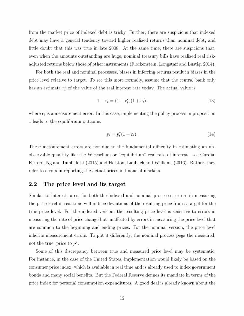
For both the real and nominal processes, biases in inferring returns result in biases in the
price level relative to target. To see this more formally, assume that the central bank only
has an estimate ret of the value of the real interest rate today. The actual value is:
1 + rt = (1 + ret )(1 + εt). (13)
where εt is a measurement error. In this case, implementing the policy process in proposition
1 leads to the equilibrium outcome:
pt = p∗t (1 + εt). (14)
These measurement errors are not due to the fundamental difficulty in estimating an un-
observable quantity like the Wicksellian or “equilibrium” real rate of interest—see Curdia,
Ferrero, Ng and Tambalotti (2015) and Holston, Laubach and Williams (2016). Rather, they
refer to errors in reporting the actual prices in financial markets.
2.2 The price level and its target
Similar to interest rates, for both the indexed and nominal processes, errors in measuring
the price level in real time will induce deviations of the resulting price from a target for the
true price level. For the indexed version, the resulting price level is sensitive to errors in
measuring the rate of price change but unaffected by errors in measuring the price level that
are common to the beginning and ending prices. For the nominal version, the price level
inherits measurement errors. To put it differently, the nominal process pegs the measured,
not the true, price to p∗.
Some of this discrepancy between true and measured price level may be systematic.
For instance, in the case of the United States, implementation would likely be based on the
consumer price index, which is available in real time and is already used to index government
bonds and many social benefits. But the Federal Reserve defines its mandate in terms of the
price index for personal consumption expenditures. A good deal is already known about the
12
(close) relationship between the two. Making the adjustment between the two should pose
no great challenge.
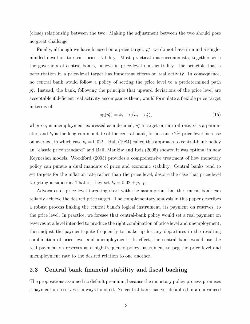
Finally, although we have focused on a price target, p∗t , we do not have in mind a single-
minded devotion to strict price stability. Most practical macroeconomists, together with
the governors of central banks, believe in price-level non-neutrality—the principle that a
perturbation in a price-level target has important effects on real activity. In consequence,
no central bank would follow a policy of setting the price level to a predetermined path
p∗t . Instead, the bank, following the principle that upward deviations of the price level are
acceptable if deficient real activity accompanies them, would formulate a flexible price target
in terms of:
log(p∗t ) = kt + α(ut − u∗t ), (15)
where ut is unemployment expressed as a decimal, u∗t a target or natural rate, α is a param-
eter, and kt is the long-run mandate of the central bank, for instance 2% price level increase
on average, in which case kt = 0.02t . Hall (1984) called this approach to central-bank policy
an “elastic price standard” and Ball, Mankiw and Reis (2005) showed it was optimal in new
Keynesian models. Woodford (2003) provides a comprehensive treatment of how monetary
policy can pursue a dual mandate of price and economic stability. Central banks tend to
set targets for the inflation rate rather than the price level, despite the case that price-level
targeting is superior. That is, they set kt = 0.02 + pt−1.
Advocates of price-level targeting start with the assumption that the central bank can
reliably achieve the desired price target. The complementary analysis in this paper describes
a robust process linking the central bank’s logical instrument, its payment on reserves, to
the price level. In practice, we foresee that central-bank policy would set a real payment on
reserves at a level intended to produce the right combination of price level and unemployment,
then adjust the payment quite frequently to make up for any departures in the resulting
combination of price level and unemployment. In effect, the central bank would use the
real payment on reserves as a high-frequency policy instrument to peg the price level and
unemployment rate to the desired relation to one another.
2.3 Central bank financial stability and fiscal backing
The propositions assumed no default premium, because the monetary policy process promises
a payment on reserves is always honored. No central bank has yet defaulted in an advanced
13
country. However, with trillions outstanding in reserves, the central bank may not have the
resources to stick to a process that promises to make payments on those reserves. Hall and
Reis (2015) discuss at length the financial stability of a central bank, and how interest-paying
reserves may put it at risk or not. Here, we apply that analysis to the case of a central bank
that follows a payment-on-reserves process.
For simplicity, assume that the central bank buys only short-term nominal government
bonds and that these never default, so they return 1 drachma next period for all states of the
world. Then, their price is 1/(1 + it). With vt denoting the outstanding amount of reserves
and bt denoting the bonds held today that are due next period, the central bank’s resource
constraint is:
vt+1 = pt+1[(1 + xt)vt − st+1 + dt+1]− bt +
(1
1 + it+1
)bt+1. (16)
Real seignorage earned from printing currency minus the expenses of running the central
bank are denoted by the net flow of revenue st in units of output. The flow of real dividends
from the central bank to the fiscal authority is denoted dt.
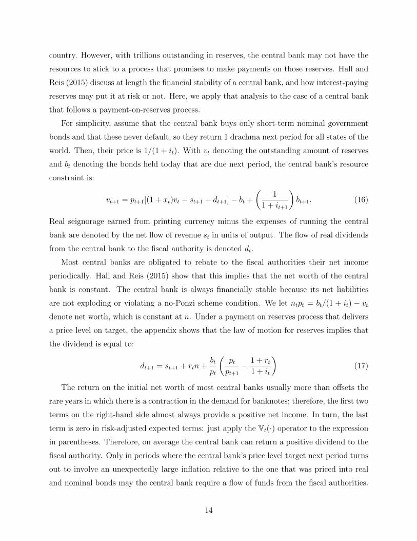
Most central banks are obligated to rebate to the fiscal authorities their net income
periodically. Hall and Reis (2015) show that this implies that the net worth of the central
bank is constant. The central bank is always financially stable because its net liabilities
are not exploding or violating a no-Ponzi scheme condition. We let ntpt = bt/(1 + it) − vtdenote net worth, which is constant at n. Under a payment on reserves process that delivers
a price level on target, the appendix shows that the law of motion for reserves implies that
the dividend is equal to:
dt+1 = st+1 + rtn+btpt
(ptpt+1
− 1 + rt1 + it
)(17)
The return on the initial net worth of most central banks usually more than offsets the
rare years in which there is a contraction in the demand for banknotes; therefore, the first two
terms on the right-hand side almost always provide a positive net income. In turn, the last
term is zero in risk-adjusted expected terms: just apply the Vt(·) operator to the expression
in parentheses. Therefore, on average the central bank can return a positive dividend to the
fiscal authority. Only in periods where the central bank’s price level target next period turns
out to involve an unexpectedly large inflation relative to the one that was priced into real
and nominal bonds may the central bank require a flow of funds from the fiscal authorities.
14

But these instances should be rare, and can be dealt with no recapitalization by maintaining
a cushion from past income or withholding future dividends.
A separate issue is whether the central bank’s monetary policy rule accords with the
support of fiscal policy in the way it pays for its deficits. It is well known that any monetary
policy is only consistent with a particular path for prices if the fiscal authority is committed
to raising fiscal surpluses to pay for increases in the nominal public debt without relying
on inflationary finance from the central bank—see Sims (2013). Throughout this paper, we
assume that the government is committed to a fiscal policy that satisfies the intertemporal
budget constraint. The payment on reserves does not modify this requirement for monetary
dominance in any significant way relative to standard treatments.
3 Price-Setting and Nominal Rigidities
So far, we have discussed the determination of the price level without any mention of who
sets prices. The price level was determined by financial markets where the values of assets
were pinned down by the forces of arbitrage. While this approach is common in the study
of price level determinacy using interest rates, such as Woodford (2003), it is worth spelling
out how it comes about in an economy with firms, workers, and goods.
3.1 Flexible prices
A widely used model with firms that set prices has firms that are monopolistically competitive
and choose their nominal price to be a constant markup over their nominal marginal costs,
which in the simple cases is equal to the nominal wage rate. On the other side of the market
are households. They supply labor to the firms up to the point where the real wage rate is
equal to the marginal rate of substitution between consumption and leisure. They consume
what is produced, as there are no savings in equilibrium, but their portfolio choices dictate
that the stochastic discount factor is equal to the intertemporal marginal rate of substitution.
Finally, they allocate spending across firms according to the relative price of their goods. If
prices are fully flexible, in this world, because all firms set the same markup in their nominal
prices over the wage rate, then real wages are just equal to the inverse of this exogenous
markup. With real wages pinned down, so is aggregate labor supply, which in turn pins
down output using the aggregate production function, and finally consumption from market
clearing in the goods market. All of these choices and real outcomes are unaffected by the
15

level of prices—the economy satisfies the classical dichotomy.
A payment-on-reserves process would work as follows in this economy. We consider the
case where the payment is indexed to the real interest rate. The central bank announces its
target for the price level, and promises a corresponding payment to the holders of reserves.
In a given period, if the candidate price level is higher than the target, a positive spread
between reserves and other real returns occurs. Investors and consumers attempt to switch
to reserves, and away from present consumption. This lowers product demand, and firms
respond by cutting prices. The price level falls and the economy finds its equilibrium at the
target price level. All this takes place in a flash of pseudo-time. The only visible price level
is equal to the price target.
3.2 Nominal rigidities
Our process is robust to different assumptions about the effects of monetary policy on real
activity. Price-level non-neutrality implies, among other things, that the economy’s real
interest rate depends on the current price level, so it is rt(pt). The dependence of the
function on time permits the history, possibly summarized by a state variable, to play a role.
The mechanisms behind rt(pt) are imperfectly understood and intensely controversial.
But the payment-on-reserves process stated in the proposition is robust to this function.
Propositions 1 to 3 in section 1 are unchanged. As long as the central bank realizes that
now rt depends on its target for the price level and adjusts the process accordingly, then it
can still implement the process in proposition 1 and achieve the price level target. Its real
payment on reserves becomes1 + rt(p
∗t )
p∗t. (18)
The logic for the global determinacy of the price level remains the same.
Things change if agents perceive that the central bank may deviate from this real payment
by some exogenous amount. Suppose that the public believes that the central bank uses the
payment-on-reserves process with a value of the real interest rate zt that may not equal the
actual market value. In this case, the price level is:
pt =1 + rt(pt)
1 + ztp∗t . (19)
Uniqueness now depends on the shape of the function rt(pt). More than one value of pt may
exist that solve this equation. Seemingly irrelevant sunspot shocks may shift the equilibrium
16

from one of these values to another, without changing zt. At this level of generality, one
cannot say more without writing a specific model of the Phillips curve. We therefore turn
to three leading models of price adjustment.
3.3 Sticky information
The sticky information model posits that firms set their prices based on stale information, as
a result of episodic updating arising from costs of updating information. In the formulation
of Mankiw and Reis (2002), every period a fraction λ ∈ (0, 1) of firms randomly drawn from
the population updates their information sets and makes plans for their future prices. The
resulting dynamic model is:
pt = λ∞∑j=0
(1− λ)jEt−j(pt + αyt) (20)
yt = Et(yt+1)−1
σrt (21)
pt − p∗t = rt − zt (22)
Hats over variables reflect their log-linear deviations from the steady state, and σ > 0 is
the intertemporal elasticity of substitution. The first equation is the Phillips curve (or AS
equation) with α > 0, while the second is the log-linearized version of the valuation operator
in equation (1) (or IS or Euler equation). The third equation refers to the payment-on-
reserves process including the exogenous shocks zt. The usual shocks in the equations of the
model, to the natural rate of interest or markups, do not affect determinacy so they can be
left out.
If there are no exogenous shocks to policy, so zt = rt, the price level is pinned to the
target by the third equation. The Phillips curve then delivers the equilibrium for yt, and
the IS curve determines rt. In the presence of a sunspot shock, the determinacy of the price
level requires an explosive dynamic response of the system to the shock. Otherwise, there
would be a continuum of equilibria indexed by the shock.
Let tildes over the variables represent the impulse responses to such a shock t periods
after. The system above implies that these responses are given by:
yt+1 = yt + (1/σ)pt (23)
(1− λ)t+1pt = α[1− (1− λ)t+1
]yt (24)
17
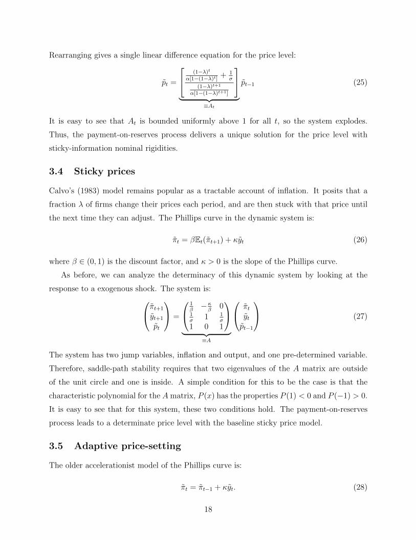
Rearranging gives a single linear difference equation for the price level:
pt =
(1−λ)tα[1−(1−λ)t] + 1
σ
(1−λ)t+1
α[1−(1−λ)t+1]
︸ ︷︷ ︸
≡At
pt−1 (25)
It is easy to see that At is bounded uniformly above 1 for all t, so the system explodes.
Thus, the payment-on-reserves process delivers a unique solution for the price level with
sticky-information nominal rigidities.
3.4 Sticky prices
Calvo’s (1983) model remains popular as a tractable account of inflation. It posits that a
fraction λ of firms change their prices each period, and are then stuck with that price until
the next time they can adjust. The Phillips curve in the dynamic system is:
πt = βEt(πt+1) + κyt (26)
where β ∈ (0, 1) is the discount factor, and κ > 0 is the slope of the Phillips curve.
As before, we can analyze the determinacy of this dynamic system by looking at the
response to a exogenous shock. The system is:πt+1
yt+1
pt
=
1β−κβ
01σ
1 1σ
1 0 1
︸ ︷︷ ︸
≡A
πtytpt−1
(27)
The system has two jump variables, inflation and output, and one pre-determined variable.
Therefore, saddle-path stability requires that two eigenvalues of the A matrix are outside
of the unit circle and one is inside. A simple condition for this to be the case is that the
characteristic polynomial for the A matrix, P (x) has the properties P (1) < 0 and P (−1) > 0.
It is easy to see that for this system, these two conditions hold. The payment-on-reserves
process leads to a determinate price level with the baseline sticky price model.
3.5 Adaptive price-setting
The older accelerationist model of the Phillips curve is:
πt = πt−1 + κyt. (28)
18

It portrays firms as setting price increases that adapt gradually to changes in output.
The analysis is similar to that of the sticky price model, so we relegate it to the appendix.
Again, the dynamic system can be written as a 3-equation system, but because now only
output is forward-looking, the condition for determinacy is that one eigenvalue is larger than
one, and the others are smaller. It is straightforward to prove that, again, the system is
determinate for any parameter values, just as in the previous two cases.
Finally, a popular model of inflation dynamics in DSGE models is a hybrid of sticky
prices and backward-looking behavior:
πt = φπt−1 + (1− φ)Et(πt+1) + κyt, (29)
where φ ∈ [0, 1]. The appendix again shows that for any value of φ, the payment-on-reserves
process leads to price-level determinacy.
4 Reserves that Provide Liquidity Services
Our propositions rely on the equality of the real cost of holding a reserve to the real present
value of its cash payoff. Reserves are priced in the same way as other financial assets, so
that from the perspective of an investor, reserves should be no different from, say, short-term
government bonds. With trillions of dollars of reserves currently outstanding, it seems rea-
sonable to assume that whatever liquidity demand for reserves is satiated, and Reis (2016a)
presents several pieces of evidence consistent with this view.
As time passes, central banks may eventually return to lean balance sheets where reserves
are scarce and earn a significant liquidity premium over other assets. And, in a financial
crisis, the demand for liquidity services provided by reserves increases so the premium may
re-emerge. This subsection studies how a payment-for-reserves process works in a world in
which the market for reserves is no longer saturated.
4.1 A general result
To take account of the liquidity services provided by reserves, we make one re-interpretation
and one modification of our general model. The re-interpretation comes from noting that
the valuation operator may depend on the real amount of reserves outstanding. We make
this dependence explicit by writing Vt(yt+1; vt/pt). Recall that vt is the quantity of reserves
19

outstanding. We show that the reserves process is robust to this modification, so our results
apply even with substantial dependence of real reserves.
Our modification adds the value of the liquidity services to the cash payoff from holding
reserves. Letting φt denote this service in drachmas, which may be random and depend on
the quantity and return on reserves, the pricing condition for reserves is now:
1 = ptVt (1 + xt; vt/pt) + φt. (30)
On the left hand side, as before, is the price of reserves, which is equal to one since they are
the unit of account. On the right-hand side is the sum of their purely financial value and
their provision of liquidity services.
With this modification, the price level is still globally uniquely determined for an exoge-
nous choice of xt. The process that delivers prices on target is modified as follows:
Proposition 4 With a liquidity premium, if the central bank sets the real payment on re-
serves to
1 + xt =(1 + rt)(1− φt)
p∗t, (31)
the unique price level is pt = p∗t .
Two lessons emerge from this proposition. The first is that, even if reserves earn a
premium return over other financial assets, as long as this premium is independent of the
price level, the payment-on-reserves process still pins down the price level uniquely. In this
case, the price level will deviate from the target in response to changes in that premium if the
policymaker does not take fluctuations in this premium into account when setting the process.
If instead the premium depends on the price level, as in the case of a non-vertical Phillips
curve discussed in the previous section, as long as the policymaker takes this dependence
into account, the payment-on-reserves process keeps the price level on target.
The second lesson is that the process is affected by the amount of reserves only via
the liquidity premium. The size of the central bank’s balance sheet may have an effect on
financial stability or on financial repression in the overall economy, and so endogenously
affects real outcomes, as in Greenwood, Hanson and Stein (2016). In our model this shows
up as the dependence of the valuation operator on the amount of reserves. But as proposition
4 shows, and all the other propositions confirmed, this does not matter for the payment-on-
reserves process. All of these effects are summarized in a sufficient statistic for price-level
20

determination: the real interest rate. Any effect of issuing more or less reserves on the
process would instead show up only directly through its effect on the size of φt.
The remainder of this section shows that the proposition above, and the lessons that fol-
low from it, are quite general: three separate standard models of these liquidity services all fit
into the formulation above. They differ only in that they provide different microfoundations
for which factors affect φt and rt.
4.2 Two old monetarist models
The most common model of the liquidity services provided by different forms of money is
the money-in-the-utility function model. It assumes that investors derive direct utility from
holding reserves as in Sidrauski’s (1967). A representative agent solves:
maxct,
vtpt,btE0
∞∑t=0
βtU
(ct,vtpt
)s.t. ptct +
bt1 + it
+ vt ≤ ptyt + bt−1 + vt−1(1 + xt−1)pt,
ct is consumption, bt bond holdings, and β < 1 is a parameter. A no-Ponzi-scheme constraint
also applies. Marginal utility with respect to reserves is strictly positive until a satiation
point after which it becomes zero.
Another popular model of liquidity assumes that a liquid asset, like reserves, provides
a means of exchange by lowering the effective costs of consumption. The problem of the
representative agent now is:
maxct,
vtpt,btE0
∞∑t=0
βtU(ct)
s.t. ptct(1− τ(vt/pt)) +bt
1 + it+ vt ≤ bt−1 + vt−1(1 + xt−1)pt,
where the function τ(·) is again strictly increasing until a satiation level and constant and
equal to 1 after that.
Both of these models are frequently used to generate a demand for liquidity. The opti-
mality conditions show that both fit into our setup above.
Lemma 1 The model of money in the utility function setup fits into our general setup with
valuation operator and liquidity premium given by:
mt+1 = βUc(ct+1, vt+1/pt+1)/Uc(ct, vt/pt) (32)
φt = Uv(ct, vt/pt)/Uc(ct, vt/pt) (33)
21
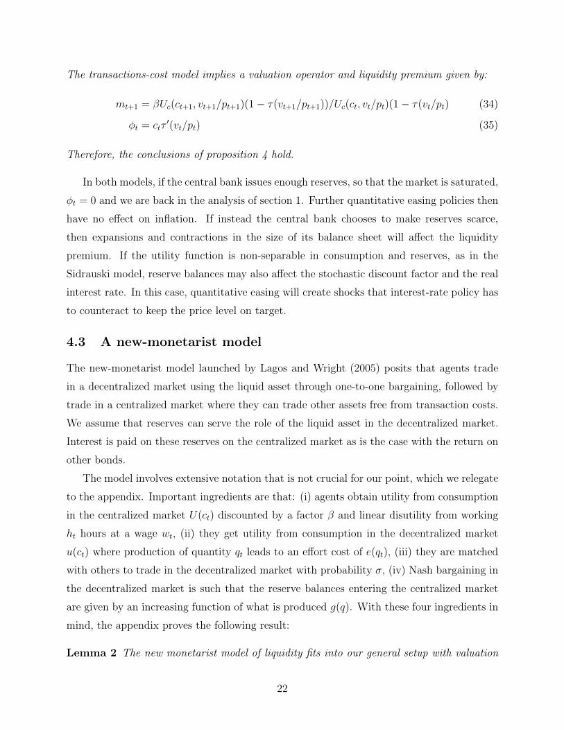
The transactions-cost model implies a valuation operator and liquidity premium given by:
mt+1 = βUc(ct+1, vt+1/pt+1)(1− τ(vt+1/pt+1))/Uc(ct, vt/pt)(1− τ(vt/pt) (34)
φt = ctτ′(vt/pt) (35)
Therefore, the conclusions of proposition 4 hold.
In both models, if the central bank issues enough reserves, so that the market is saturated,
φt = 0 and we are back in the analysis of section 1. Further quantitative easing policies then
have no effect on inflation. If instead the central bank chooses to make reserves scarce,
then expansions and contractions in the size of its balance sheet will affect the liquidity
premium. If the utility function is non-separable in consumption and reserves, as in the
Sidrauski model, reserve balances may also affect the stochastic discount factor and the real
interest rate. In this case, quantitative easing will create shocks that interest-rate policy has
to counteract to keep the price level on target.
4.3 A new-monetarist model
The new-monetarist model launched by Lagos and Wright (2005) posits that agents trade
in a decentralized market using the liquid asset through one-to-one bargaining, followed by
trade in a centralized market where they can trade other assets free from transaction costs.
We assume that reserves can serve the role of the liquid asset in the decentralized market.
Interest is paid on these reserves on the centralized market as is the case with the return on
other bonds.
The model involves extensive notation that is not crucial for our point, which we relegate
to the appendix. Important ingredients are that: (i) agents obtain utility from consumption
in the centralized market U(ct) discounted by a factor β and linear disutility from working
ht hours at a wage wt, (ii) they get utility from consumption in the decentralized market
u(ct) where production of quantity qt leads to an effort cost of e(qt), (iii) they are matched
with others to trade in the decentralized market with probability σ, (iv) Nash bargaining in
the decentralized market is such that the reserve balances entering the centralized market
are given by an increasing function of what is produced g(q). With these four ingredients in
mind, the appendix proves the following result:
Lemma 2 The new monetarist model of liquidity fits into our general setup with valuation
22

operator and liquidity premium given by:
mt+1 = βU ′(ct+1)/U′(ct) (36)
φt =
(σβ
U ′(ct)
)Et(u′(qt+1)− e′(qt+1)
g′(qt+1)
)(37)
Therefore, the conclusions of proposition 4 hold.
The liquidity premium in this model arises from the effect that carrying reserves has
on the terms of trade in the decentralized market on the incentives facing consumers and
producers. The central bank could drive this term to zero by saturating the market with
reserves. The payment-on-reserves process delivers a unique price level.
5 Segmented Financial Markets
Reserves are a special asset. They are the unit of account, they never default, and the central
bank controls both their quantity as well as their remuneration. These special properties
enable the payment-on-reserves process to control the price level.
One other special feature of reserves in most advanced economics is that only financial in-
stitutions can hold them. In the United States, only banks can hold reserves, but since 2014,
a broader set of financial institutions can also lend to the Fed in the overnight repurchase
agreement market on terms that the Fed sets. The new asset, called an RRP, is effectively
a reserve, and implementing our payment-on-reserves process in the United States would be
done by having an equivalent payment on RRPs.
As long as these financial institutions compete for arbitraging away differences in returns
between reserves and safe short-term bonds, then our results apply. This section studies the
unlikely, but possible, case where this may not happen because of financial frictions in the
financial sector that lead to a segmentation between the markets for bonds and for reserves.
5.1 A general setup
Segmented markets between two assets lead to positive or negative premiums in their returns.
One way to model segmentation is to posit that the valuation operator that applies to reserves
is different from the one that applies to bonds. With segmentation, the two separate values
can co-exist because there are no agents able to arbitrage the valuation disparity. Another
way to interpret segmentation posits that the financial institutions that can hold reserves
23

have a valuation operator different from the agents that bonds. We do not think this is
likely, but this section serves as a robustness check, and it fits into some of the models of
banks and financial frictions in the literature.
We introduce a new valuation operator Vbt(·) for banks, the holders of reserves. The
equilibrium condition for reserves with a payment-on-reserves process becomes:
1 = ptVbt(1 + xt). (38)
Because this valuation operator differs from the one for indexed bonds. it is no longer the
case that Vbt(1) is equal to the inverse of the gross real interest rate. Instead, we define the
value premium of reserves as:
1 + χt ≡ Vbt(1)(1 + rt). (39)
This may be positive or negative and it may even vary over time, as the inability of agents
to arbitrage this premium away may depend on the evolution of the economy.
Combining the two expressions above leads to a simple modification of our main result:
Proposition 5 With a reserves value premium, if the central bank sets the real payment on
reserves to
1 + xt =(1 + rt)
(1 + χt)p∗t, (40)
the unique price level is pt = p∗t .
Again, this modification poses no theoretical constraint on the ability of the central bank to
determine the price level. If the central bank has difficulties measuring the value premium,
then these estimation errors will lead to some discrepancy between target and actual prices.
These discrepancies are likely of the same order as those arising from mismeasuring the
natural rate of interest in the conventional application of the Taylor rule. Moreover, with the
wealth of data on interbank markets and on spreads between interest rates in those markets
and in treasury bills, repo, and other money markets, there is no lack of real time data with
which to measure χt and to adjust the payment-on-reserves process to these spreads.
5.2 Three micro-founded models of banks and reserves
Many standard models of banking fit into the general setup we just described. This subsec-
tion briefly describes three of them.
24

5.2.1 Banks and costly state verification
The costly state-verification assumption, as employed by Bernanke, Gertler and Gilchrist
(1999), is an element of many models of credit frictions. In this model, an entrepreneur
has limited net worth to finance its capital investment, which has a random payoff that is
private information of the entrepreneur. At some cost, the state can be revealed to financiers.
The optimal contract involves such a disclosure for a limited set of states. Bernanke and
coauthors’ tractable formulation shows that overall investment will increase proportionally
with net worth, while the aggregate supply of external finance increases with the external-
finance spread between the return on capital and the return earned by the financier.
Reserves held by banks need no such monitoring, since they are always honored by the
central bank. There are then two ways to think of banks in this setup. One is to view the
bank as the financier, collecting deposits from households and lending them to entrepreneurs.
In that case, with a banking sector that is competitive, the return on deposits is the same as
the return on reserves. Because households can deposit funds with banks or buy government
bonds, the return on deposits is the same as the return on bonds. In this case, there is no
value premium: χt = 0. A second way is to think of banks as the entrepreneurs, who are
being monitored by depositors. In that case, the return on reserves is equated to the return
on capital. It exceeds the return on bonds by the external-finance spread. In that case, χt
is equal to this external-finance spread.
5.2.2 Banks and limited commitment
A more recent model of banks focuses on the inability of banks to commit not to divert a
share of the funds given to them by depositors. Gertler and Kiyotaki (2010) is a prominent
example of this approach, which has also been incorporated in many models of monetary
policy and inflation. In this model, bankers only repay the depositor if the value of staying
in business is at least as large as the value from running away with a fraction of the current
assets. A bank is able to collect more deposits if it has higher net worth, since a fraction of
that net worth would be lost in case of default. At the same time, leverage is constrained
by the limited amount of skin in the game that banks can pledge given their limited capital.
This constraint gives rise to a positive spread between the return the bank can earn on its
projects and the return it pays to depositors. This spread captures the marginal unit value
of having extra net worth to the bank by relaxing its leverage constraint.
25

Again, there are two ways to view reserves in this setup, depending on whether the
defaulting banker can run away with reserves or not. Of course deposits at the central bank
could be seized by creditors, but a bank can instantly convert reserves to cash at the central
bank and cash is anonymous and easier to abscond with. So, which case one takes depends
on view on how quickly the bank could convert reserves into banknotes and escape with
them. In the case where reserves can be fully seized by creditors, then their return will be
equated to the return paid to depositors, in which case χt = 0. In the case where reserves
can only be partially seized, then their return will be equated to the return on the other
assets of the bank, and like them earns a premium χt, which now reflects the inability of
banks to scale up their investments because of the limited commitment problem.
5.2.3 Banks and fiscal default
Reis (2016b) notes that reserves and government bonds behave differently in a fiscal crisis.
While governments often default on the government bonds they issue, central banks almost
never default on reserves. Because reserves are the unit of account, defaulting on them
requires a reform of the currency and monetary system in the country. Of course, unexpected
inflation is a way to equally reduce the payments on both reserves and government bonds.
Because banks can hold reserves, they have access to a safe asset in a fiscal crisis that
other agents in the economy do not. A recent literature has emphasized the scarcity of safe
assets in modern economies, which are needed for instance to use as collateral in financial
transactions—see Gorton, Lewellen and Metrick (2012) and Caballero, Farhi and Gourinchas
(2016). Banks will value their ability to hold reserves to relax their financial constraints.
In this case, the value premium χt has two origins. First, it is a sovereign default pre-
mium that government bonds must pay but reserves do not. Second, it captures the marginal
relaxation of banks’ financial constraints that reserves provide during a fiscal crisis. In the
case of the United States, both are likely small, so χt = 0 for the Federal Reserve. For the
ECB instead, there is significant cross-country variation in χt, which can be approximately
measured in different ways using sovereign spread, credit default swaps and many other fi-
nancial prices, for example, Krishnamurthy, Nagel and Vissing-Jorgensen (2014). Measuring
this premium and adjusting monetary policy to it has already for the past few years been a
source of focus and research by the ECB in managing the monetary transmission mechanisms
in the Euro area.
26
6 Relation to the Literature
Hall (1997) appears to be the first statement of the idea that reserves could take the form of
a security whose purchasing power is designed to be constant, though he noted that Irving
Fisher proposed that the monetary unit could be a quantity of gold adjusted continuously
to keep its purchasing power constant. Hall transplanted that idea to a security, an im-
plementation more harmonious with modern monetary institutions. He then observed that,
in continuous time, a floating-rate note paying the current real interest rate always has a
purchasing power of one, so letting that note be the monetary unit would result in a price
level of one at all times.
Relative to Hall, we have shown in discrete time that promising a payment on reserves,
which are one-period assets, can accomplish any desired price level p∗. The economic logic
of why this works is the same: If the price level deviate from p∗, a valuation anomaly occurs.
But the payment-on-reserves process is a more natural policy within the new-style of central
banking, it is easier to implement, and it flexibly allows for an elastic price or inflation
standard.
Hall (2002) also discusses the Chilean Unidad de Fomento, which is a parallel monetary
unit with strictly constant purchasing power. It is defined as enough pesos to buy the cost
of living bundle. Our process stabilizes the purchasing power of the transactional monetary
unit, not a parallel unit. Moreover, our process makes clearer that the economic logic behind
it is different from that of the gold standard, or any other commodity standard. In effect,
we provide an affirmative answer to a question that has been raised about the UF—is there
some way that the UF could become the single monetary unit of Chile?
6.1 Relation to interest-rate rules
A huge literature examines the conditions for determinacy of the price level, a surprisingly
subtle issue. Cochrane (2011) contains a recent lengthy discussion, while Woodford (2003)
is the classic reference. With a payment-on-reserves process, the price level is pinned exactly
on target each period. Unlike the Taylor rule, it does not generate a difference equation
describing potential equilibrium price trajectories that must be iterated over time to infinity
and paired with some controversial boundary condition—see the discussion in Cochrane
(2016).
The literature on interest-rate rules also relies on the no-arbitrage condition between
27

reserves and government bonds. But, in our case, only no-arbitrage between two successive
periods is needed, not across an infinite number of them. Therefore, concerns about how
agents form expectations far into the future, which are crucial for determinacy with interest-
rate rules, do not apply to our process—see Garcia-Schmidt and Woodford (2015) and Gabaix
(2016). Our process also does not rely on linearizations, but they play an important role
with interest-rate rules, as discussed by Benhabib, Schmitt-Grohe and Uribe (2002) and
Christiano, Eichenbaum and Johannsen (2016). Finally, as we showed in section 4, the precise
way in which reserves affect liquidity does not affect determinacy, unlike what happens with
interest-rate rules (Schmitt-Grohe, Benhabib and Uribe, 2001).
Two papers in the Wicksell- and Taylor-rule tradition are closer to our process. Adao,
Correia and Teles (2011) consider an interest-rate process where the central bank follows the
log-linearized rule:
it = rt + Et(pt+1)− p∗t . (41)
They pair this rule with a log-linearized Fisher equation relating nominal and real interest
rates,
it = rt + Et(pt+1)− pt. (42)
The only possible outcome is p = p∗. Loisel (2009) discusses a similar monetary policy rule
in the context of a broader treatment of policy rules.
As these authors showed, these rules are fragile: If the policy interest rate responds
to Et(pt+1) with a coefficient that even slightly deviates from one, then there are multiple
explosive solutions for the price level. With a payment-on-reserves process instead, the price
level is robustly pinned to the target and depends only on the easy-to-observe market interest
rate. Expectations of future prices are already included in the nominal rate, so the central
bank does not need to form or observe any forecasts.
6.2 Relation to fiscal and monetary theories
The fiscal theory of the price level also has some similarities with our approach as well as
important differences. In that theory, the treasury issues nominal liabilities, which, via the
government budget constraint, have a fixed real payoff in terms of expected present fiscal
surpluses. In our setup, it is the central bank that issues a nominal liability, and it chooses
the real payoff using the payment-on-reserves process. As Cochrane (1998) emphasizes, the
fiscal theory of the price level can also be interpreted in terms of a no-arbitrage principle, like
28

with our process, in the valuation of government bonds as claims on the finite stream of fiscal
surpluses. But our process does not have to appeal to the government budget constraint as
an equilibrium object; the central bank controls the real payment on reserves directly.
With the payment-on-reserves process, control of the price level remains with the mone-
tary authority, so there is ‘monetary dominance. Our process does not rely on non-Ricardian
behavior by the fiscal authorities. The process can co-exist with concerns about fiscal backing
of the central bank and coordination between fiscal and monetary policy—see Sims (2013).
Finally, relative to an older monetarist tradition dating back to Cagan (1956), our ap-
proach does not rely on there being a stable demand for money. It is perfectly consistent
with the existence of a demand for liquidity, but it relies on a different mechanism to pin
down the price level.
7 Conclusion
This paper proposes a new approach for central banks to control the price level. As in all
theories of the price level, ours relies on the properties of a nominal government liability.
Our novelty is to focus on reserves, which are the unit of account, default-free, voluntarily
held by banks, and with remuneration set by the central bank as its policy instrument.
Within the class of theories of price-level determination focusing on the central bank’s
control of an interest rate, the key economic force at play is an arbitrage condition in financial
markets. Our novelty is to observe that by setting a payment on those reserves, arbitrage
between one period and the next will pin down the price level, without needing to consider
arbitrage into the infinite future. As in post financial-crisis work in macroeconomics, but
almost absent from the price-level determination literature, we consider the role played by
liquidity and credit frictions in financial markets. Together with mis-measurement of prices
and returns, we show that it is easy to adapt our policy process to their presence.
This approach provides three equivalent policy proposals for a central bank. They all
consist in announcing a payment on reserves, but differ only on whether that payment is
stated in units of output, is indexed to the price level, or is stated in nominal terms. For each
of them there is an easy-to-implement policy process that delivers a unique price level. We
showed that this uniqueness is global. Moreover, the control errors in hitting the target can
be linked to measurement errors on actual prices and interest rates, instead of theoretical
objects such as the natural real interest rate. Therefore, we believe that our approach has
29

practical policy advantages relative to the existing practices of central banks.
We note that we have not provided an account of how the price level gets from some
arbitrary initial value to the equilibrium p∗. Our process is therefore subject to the “unso-
phisticated implementation” critique of Atkeson, Chari and Kehoe (2010), because we have
not described how the economy behaves when the price level deviates from p∗. The topic is
essentially an old one, the “channels of monetary policy.”
We think that a story could be fashioned along conventional lines, with the following gist.
Suppose the central bank finds that the price-level forecast lies above the target associated
with the current level of real activity, so some contraction is in order. The bank raises the real
payment on reserves. Immediately, other short-run real rates rise to preserve no-arbitrage
across assets. In the presence of price-level non-neutrality, the central bank controls all
short-term real rates, just as in standard models. Higher real rates result in lower spending
and a slack economy. The economy makes its way to a point where the price-level forecast
and the level of real activity satisfies the elastic price standard.
Rigorously modeling the process sketched above using modern tools, following Bassetto
(2002), would require many extra simplifications. In turn, the story would have to deal with
all the contentious issues of modern fluctuations theory.
30

References
Adao, Bernardino, Isabel Correia, and Pedro Teles, “Unique monetary equilibria with in-
terest rate rules,” Review of Economic Dynamics, 2011, 14 (3), 432–442.
Atkeson, Andrew, Varadarajan V. Chari, and Patrick J. Kehoe, “Sophisticated Monetary
Policies,” Quarterly Journal of Economics, 2010, 125 (1), 47–89.
Ball, Laurence, N. Gregory Mankiw, and Ricardo Reis, “Monetary Policy for Inattentive
Economies,” Journal of Monetary Economics, May 2005, 52 (4), 703–725.
Bassetto, Marco, “A Game-Theoretic View of the Fiscal Theory of the Price Level,” Econo-
metrica, 2002, 70 (6), 2167–2195.
Benhabib, Jess, Stephanie Schmitt-Grohe, and Martin Uribe, “Avoiding Liquidity Traps,”
Journal of Political Economy, June 2002, 110 (3), 535–563.
Bernanke, Ben S., Mark Gertler, and Simon Gilchrist, “The Financial Accelerator in a
Quantitative Business Cycle Framework,” in John B. Taylor and Michael Woodford,
eds., Handbook of Macroeconomics, Elsevier, 1999, chapter 21, pp. 1341–1393.
Caballero, Ricardo J., Emmanuel Farhi, and Pierre-Olivier Gourinchas, “Safe asset scarcity
and aggregate demand,” American Economic Review, May 2016, 106 (5), 513–18.
Cagan, Phillip, “The Monetary Dynamics of Hyperinflations,” in Milton Friedman, ed.,
Studies in the Quantity Theory of Money, The University of Chicago Press, 1956, pp. 25–
117.
Calvo, Guillermo A., “Staggered Prices in a Utility-Maximizing Framework,” Journal of
Monetary Economics, September 1983, 12 (3), 383–398.
Christiano, Lawrence J., Martin Eichenbaum, and Benjamin K. Johannsen, “Does the New
Keynesian Model Have a Uniqueness Problem?,” June 2016. Northwestern University
manuscript.
Cochrane, John H., “A Frictionless View of U.S. Inflation,” NBER Macroeconomics Annual,
1998, 13 (1), 323–421.
31

, “Determinacy and Identification with Taylor Rules,” Journal of Political Economy,
2011, 119 (3), 565–615.
, “The New Keynesian Liquidity Trap,” June 2016. Hoover Institution, Stanford
University.
Curdia, Vasco, Andrea Ferrero, Ging Cee Ng, and Andrea Tambalotti, “Has U.S. monetary
policy tracked the efficient interest rate?,” Journal of Monetary Economics, 2015, 70,
72–83.
Fleckenstein, Matthias, Francis Longstaff, and Hanno Lustig, “The TIPS-Treasury Bond
Puzzle,” Journal of Finance, September 2014, 69 (5), 2151–2197.
Gabaix, Xavier, “A Behavioral New Keynesian Model,” October 2016. NYU manuscript.
Garcia-Schmidt, Mariana and Michael Woodford, “Are Low Interest Rates Deflationary? A
Paradox of Perfect-Foresight Analysis,” NBER Working Paper 21614 October 2015.
Gertler, Mark and Nobuhiro Kiyotaki, “Financial Intermediation and Credit Policy in Busi-
ness Cycle Analysis,” in Benjamin M. Friedman and Michael Woodford, eds., Handbook
of Monetary Economics, Vol. 3 of Handbook of Monetary Economics, Elsevier, January
2010, chapter 11, pp. 547–599.
and Peter Karadi, “QE 1 vs. 2 vs. 3...: A Framework for Analyzing Large-Scale
Asset Purchases as a Monetary Policy Tool,” International Journal of Central Banking,
January 2013, 9 (1), 5–53.
Goodfriend, Marvin, “Central banking under the gold standard,” Carnegie-Rochester Con-
ference Series on Public Policy, 1988, 29, 85 – 124.
Gorton, Gary, Stefan Lewellen, and Andrew Metrick, “The Safe-Asset Share,” American
Economic Review, May 2012, 102 (3), 101–06.
Greenwood, Robin, Samuel G. Hanson, and Jeremy C. Stein, “The Federal Reserve’s Balance
Sheet as a Financial-Stability Tool,” in “Designing Resilient Monetary Policy Frame-
works for the Future,” Jackson Hole Symposium: Federal Reserve Bank of Kansas City,
August 2016.
32

Hall, R. E., “Controlling the Price Level,” Contributions to Macroeconomics, 2002, 2 (1).
Hall, Robert E., “Monetary Strategy with an Elastic Price Standard,” in “Price Stability
and Public Policy: A Symposium Sponsored by the Federal Reserve Bank of Kansas
City” 1984.
, “Irving Fisher’s Self-Stabilizing Money,” American Economic Review Papers and
Proceedings, May 1997, 87 (2), 436–438.
and Ricardo Reis, “Maintaining Central-Bank Solvency under New-Style Central Bank-
ing,” NBER Working Paper 21173 July 2015.
Holston, Kathryn, Thomas Laubach, and John Williams, “Measuring the Natural Rate of
Interest: International Trends and Determinants,” in “NBER International Seminar on
Macroeconomics 2016,” National Bureau of Economic Research, Inc, Jan-Jun 2016.
Krishnamurthy, Arvind, Stefan Nagel, and Annette Vissing-Jorgensen, “ECB Policies in-
volving Government Bond Purchases: Impact and Channels,” August 2014. Stanford
University.
Lagos, Ricardo and Randall Wright, “A Unified Framework for Monetary Theory and Policy
Analysis,” Journal of Political Economy, June 2005, 113 (3), 463–484.
Loisel, Olivier, “Bubble-free policy feedback rules,” Journal of Economic Theory, 2009, 144
(4), 1521–1559.
Mankiw, N. Gregory and Ricardo Reis, “Sticky Information versus Sticky Prices: A Pro-
posal to Replace the New Keynesian Phillips Curve,” Quarterly Journal of Economics,
November 2002, 117 (4), 1295–1328.
Reis, Ricardo, “Funding Quantitative Easing to Target Inflation,” in “Designing Resilient
Monetary Policy Frameworks for the Future,” Jackson Hole Symposium: Federal Re-
serve Bank of Kansas City, August 2016.
, “QE in the future: the central bank’s balance sheet in a fiscal crisis,” NBER Working
Paper 22415 June 2016.
Schmitt-Grohe, Stephanie, Jess Benhabib, and Martin Uribe, “Monetary Policy and Multi-
ple Equilibria,” American Economic Review, March 2001, 91 (1), 167–186.
33
Sidrauski, Miguel, “Rational Choices and Patterns of Growth in a Monetary Economy,”
American Economic Review, Papers and Proceedings, 1967, 57, 534–544.
Sims, Christopher A., “Paper Money,” American Economics Review Papers and Proceedings,
May 2013, 103 (3), 563–584.
Woodford, Michael, Interest and Prices, Princeton, New Jersey: Princeton University Press,
2003.
34

Appendixes
A Financial Stability with a Constant-Net-Worth Rule
If the central bank’s independence mandate requires it to choose dividends dt such that the
net worth of the central bank is constant, then nt = nt+1 implies that:
−vt+1
pt+1
+bt+1
(1 + it+1)pt+1
= nt.
The law of motion for reserves in equation equation (16) can be rearranged as follows:
vt+1
pt+1
− bt+1
pt+1(1 + it+1)= (1 + xt)vt − st+1 + dt+1 −
btpt+1
.
Adding both sides of these equations gives the solution for dividends:
dt+1 = st+1 + rtnt − (1 + rt)nt − (1 + xt)vt +btpt+1
.
Recalling the definition of nt in terms of assets and liabilities and rearranging gives:
dt+1 = st+1 + rtnt −btpt
(1 + rt1 + it
− ptpt+1
)+ [1 + rt − (1 + xt)pt]
(vtpt
).
Finally, note that the last term is zero under the payment-on-reserves process for monetary
policy. This gives the desired result in equation (17).
B Determinacy Proofs
For the Calvo sticky price model, the characteristic polynomial is:
P (x) = x3 −(
2 +1
β
)x2 + [1 +
2
β+
κ
βσ]x− 1
β.
It is easy to see that P (1) = −κ/(σβ) < 0 while P (−1) = 4 + 4/β + κ/(βσ) > 0. Therefore,
the system has two eigenvalues outside the unit circle, and one inside: the condition for
saddle path stability.
Turn next to the accelerationist model. In matrix notation, the system is: yt+1
πtpt
=
1 + κ/σ 1/σ 1/σκ 1 0κ 1 1
︸ ︷︷ ︸
A
ytπt−1pt−1
35

There is one non-predetermined variable, yt, and two endogenous predetermined variables,
πt and pt−1. Thus, for the system to have a unique solution it is required that the matrix A
has one eigenvalue outside the unit circle and two inside.
The characteristic polynomial of the matrix is:
P (x) = x3 + [−(2 + β)− κ
σ]x2 + (1 + 2β)x− β
and we need to check that one of its roots is above 1, and the other two are below one in
absolute value. Make the transformation: x = (1 + s)/(1− s). The polynomial becomes:
P (s) = s3 +
(4(1− β) + κ
σ
4(1 + β) + κσ
)s2 −
(κ
(4(1 + β) + κσ)σ
)s−
(κ
(4(1 + β) + κσ)σ
)and determinacy is now equivalent to this polynomial having one positive and two negative
roots. Descartes’s rule of sign shows that this is the case independently of parameters because
the coefficient signs of P (s) are + + −−, so there is one positive root, and the coefficient
signs of P (−s) are = −+ +− implying two negative roots.
The case for the hybrid Phillips curve is almost identical, so we state only the A matrix:
A ≡ 1
(1− φ)σβ
σ −σκ −φσ 0
(1− φ)β (1− φ)σβ 0 (1− φ)β0 0 (1− φ)σβ 0
(1− φ)σβ 0 0 (1− φ)σβ
.The characteristic polynomial after the x = (1 + s)/(1− s) transformation is:
P (s) =
(4 +
4(1 + φ)
β(1− φ)+
κ
βσ(1− φ)
)s4 + 8
(β(1− φ)− φβ(1− φ)
)s3
−(κ+ 2σ(1− φ)(1− β)
βσ(1− φ)
)s2 +
κ
βσ(1− φ)
Because there are two forward-looking variables, and two perdetermined ones, for determi-
nacy there should be two positive and two negative roots. The signs of the coefficients for
P (s) are +?−+ so there are two positive roots according to Descartes’ sign rule. They are
+?−+ for P (−s) implying two negative roots.
C The New Monetarist Model
In the centralized market, the representative household solves:
V CM(vt, bt) = maxct,ht,vt,bt
{U(ct)− ht + β Et
[V DM(vt+1, bt+1
]}s.t. ptct +
bt1 + it
+ vt ≤ ptwtht + bt−1 + pt(1 + xt−1)vt + Tt
36

where vt are the outstanding reserve balance of an agent entering the centralized market.
This leads to the first-order conditions:
U ′(ct)− λtpt = 0
λtPtwt − A = 0
λt = β Et[V DMv (vt+1, bt+1)
]λt = β Et
[V DMb (vt+1, bt+1)
]V CMv (vt, bt) = pt(1 + xt−1)λt
V CMb (vt, bt) = (1 + it−1)λt
In the decentralized market, with probability σ a household is assigned to one side of the
decentralized market (i.e. buyer or seller) and with probability (1 − 2σ) it is inactive. The
value of entering the decentralized market then is:
V DM(vt, bt) = σ[χu(qt) + V CM(vt − dvt , bt)
]+ σ
[−e(qt) + V CM(dvt + vt, bt)
]+ (1− 2σ)V CM(vt, bt)
The inverse production function is et = e(qt). From this it follows that:
V DMv (vt, bt) = V CM
v (vt, bt) + σ
[χu′(qt)
∂qt∂vt− V CM
v (vt, bt)∂dv
∂vt
]+ σ
[−e′q(qt)
∂qt∂vt
+ V CMv (vt, bt)
∂dv
∂vt
]V DMb (vt, bt) = V CM
b (vt, bt)
Finally, when the representative buyer and the representative seller in the decentralized
market meet, they make a Nash bargain:
maxqt,dvt
[χu(qt)− U ′(ct)
dvtpt
]θ [U ′(ct)
dvtpt− e(qt)
]1−θs.t. dvt ≤ vbt
Defining:
g(q) =(1− θ)e′q(q)χu(q) + θχu′(q)e(q)
θχu′(q) + (1− θ)e′q(q)the optimality condition from the Nash bargaining problem together with the equilibrium
condition that all the reserves are used for purchases becomes:
v = dv = g(q)pw.
From this it follows that ∂dv/∂v = 1 and ∂q/∂v = 1/wpg′q(q)
37
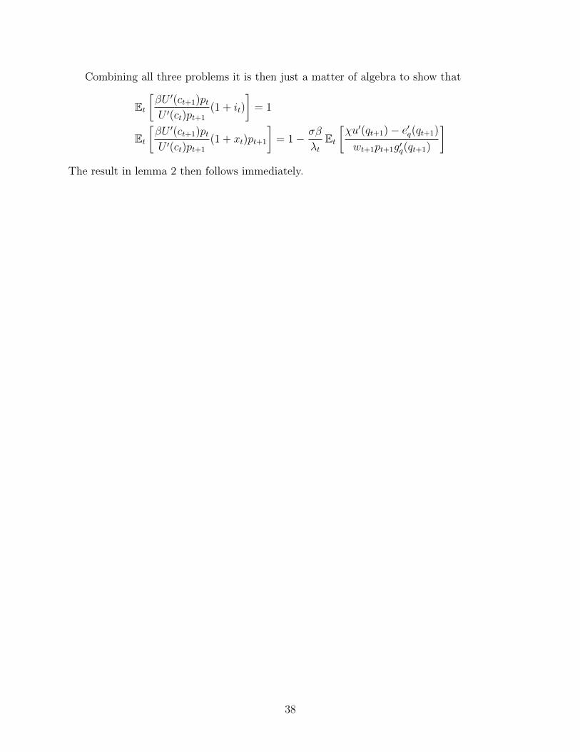
Combining all three problems it is then just a matter of algebra to show that
Et[βU ′(ct+1)ptU ′(ct)pt+1
(1 + it)
]= 1
Et[βU ′(ct+1)ptU ′(ct)pt+1
(1 + xt)pt+1
]= 1− σβ
λtEt[χu′(qt+1)− e′q(qt+1)
wt+1pt+1g′q(qt+1)
]The result in lemma 2 then follows immediately.
38