achieving near-optimal mimo capacity in a rank...

ACHIEVING NEAR-OPTIMAL MIMO CAPACITY IN A

RANK-DEFICIENT LOS ENVIRONMENT

A Dissertation

Presented to

The Academic Faculty

By

Brett T. Walkenhorst

In Partial Fulfillment

of the Requirements for the Degree

Doctor of Philosophy in Electrical Engineering

School of Electrical and Computer Engineering

Georgia Institute of Technology

August 2009

Copyright © 2009 by Brett T. Walkenhorst

ii

ACHIEVING NEAR-OPTIMAL MIMO CAPACITY IN A

RANK-DEFICIENT LOS ENVIRONMENT

Approved by:

Dr. Mary Ann Ingram, Advisor School of Electrical and Computer Engineering Georgia Institute of Technology

Dr. Gregory D. Durgin School of Electrical and Computer Engineering Georgia Institute of Technology

Dr. Ye Li School of Electrical and Computer Engineering Georgia Institute of Technology

Dr. John J. Landgren Georgia Tech Research Institute Georgia Institute of Technology

Dr. J. Stevenson Kenney School of Electrical and Computer Engineering Georgia Institute of Technology

Date Approved: June 24, 2009

iii

To my wife Emily

and our four children.

iv

Acknowledgements

There are many people who have helped to inspire and encourage me in pursuing this degree.

To my wife Emily goes all the gratitude of my heart. Without her help, I would not be where I am today. I

don’t have room in this paper to express my appreciation for her or describe how I feel about her;

however, without her, I am confident I could not have achieved the success I have experienced in my

schooling or in my career. Whatever honors are due to me, she has earned them right along with me.

Thank you.

I also owe a great deal to my friend and former colleague Dr. Tom Pratt, one of the kindest men

I have ever known. Our discussions and his guidance and encouragement have been incredibly valuable

to my sanity and success. If I have earned the bestowal of a PhD, a great deal of the credit for my

success goes to him.

Thanks go to my supervisor Eric Barnhart for his support in so many ways and his constant

vigilance in looking for opportunities to help me in my career and in pursuing the PhD degree. He is an

excellent manager and a good man.

I appreciate the faith and funding of the GTRI Fellows Council in giving me an opportunity to

pursue the research that led to the initial findings for this dissertation. To Dr. Ron Bohlander and the

other Fellows go my sincere appreciation for the opportunity and encouragement they gave me to look

at MIMO limitations in a LOS environment. I also appreciate the faith and support of others including

Paul Burns, Dr. Margaret Loper, Dr. Randy Case, Dr. Bill Melvin, and others that led to funding that

helped me finalize my research.

To many others go my gratitude for valuable discussions and insights, some of which were

directly related to this research, others of which were helpful to me personally and/or professionally

along the way. To Dr. Jack Landgren, Jeff Evans, Darryl Sale, Dr. Bob Baxley, and many others at GTRI,

v

thank you for the many interesting and enlightening discussions and for your support, encouragement,

and insights.

To my academic advisor, Dr. Mary Ann Ingram, go my thanks for the countless hours coaching

me and guiding me through my research and helping me to develop my analytical skills. She was always

willing to give me whatever time I needed. I am a better man for my association with her and for what I

have learned from her. I have enjoyed our discussions, both technical and otherwise, but more

important than her guidance has been her encouragement. Perhaps more than anyone else, she has

helped me to feel that I was capable of accomplishing this. She is one of the most genuinely kind

individuals I know.

Most importantly, my thanks go to God. Without His promptings, I would not have begun the

pursuit of this degree and without His help, I’m certain I could not have completed it. I’m confident that

I am not capable of repaying what I owe Him, but I’ll do my best.

vi

Table of Contents

Acknowledgements ___________________________________________________________ iv

List of Tables _________________________________________________________________ ix

List of Figures _________________________________________________________________x

List of Acronyms _____________________________________________________________ xiii

Parameter Definitions ________________________________________________________ xiv

Summary ___________________________________________________________________ xvi

Chapter 1: Introduction ________________________________________________________ 1

Chapter 2: Origin and History of the Problem _______________________________________ 4

2.1. LOS MIMO __________________________________________________________________ 4

2.2. LOS Channel Matrix Study _____________________________________________________ 6

2.3. Repeaters for MIMO Capacity Enhancement ______________________________________ 6

2.4. Current Repeater Usage _______________________________________________________ 6

2.5. Cooperative Communications __________________________________________________ 7

Chapter 3: Analyzing the Channel Matrix Form _____________________________________ 9

3.1. LOS MIMO _________________________________________________________________ 10

3.2. Hadamard’s Maximum Determinant Problem ____________________________________ 11

3.3. A Geometric Interpretation ___________________________________________________ 13

3.4. A 2x2 Example _____________________________________________________________ 14

3.5. Higher-Order MIMO Considerations ____________________________________________ 16

3.6. Simulation Results __________________________________________________________ 17

Chapter 4: MIMO Bounds as a Function of the Determinant Metric ____________________ 22

4.1. A Generalized Determinant-Based Metric _______________________________________ 23

4.2. Bounding the Metric ________________________________________________________ 23

4.2.1. Fixed Instantaneous SNR __________________________________________________________ 23

4.2.2. Fixed Average SNR _______________________________________________________________ 28


Chapter 5: RACE for Fixed Point-to-Point LOS MIMO Links ___________________________ 34

5.1. Channel Model _____________________________________________________________ 35

5.2. Repeater Model ____________________________________________________________ 36

vii

5.3. 2x2 Repeater Position Analysis ________________________________________________ 37

5.3.1. Optimal Inter-Element Spacing _____________________________________________________ 39

5.3.2. Free Space Repeater Positioning ___________________________________________________ 39

5.3.3. Repeater Positioning with Multipath ________________________________________________ 42

5.3.4. Variations in and ____________________________________________________________ 44

5.3.5. Three-Dimensional Repeater Positioning Analysis _____________________________________ 46

5.4. A 2x2 Repeater Position Metric ________________________________________________ 48

5.5. Repeater Power and Delay Spread _____________________________________________ 50

5.5.1. Repeater Power Analysis _________________________________________________________ 50

5.5.2. Delay Spread Analysis ____________________________________________________________ 51

5.6. Discussion _________________________________________________________________ 52

Chapter 6: Higher Order MIMO _________________________________________________ 53

6.1. Introduction _______________________________________________________________ 53

6.2. Sufficient Conditions ________________________________________________________ 54

6.3. Approximate Channel Model __________________________________________________ 55

6.4. Sufficiency Proof ____________________________________________________________ 56

6.5. A 4x4 Example _____________________________________________________________ 58

6.6. Suboptimal Repeater Placement _______________________________________________ 61

6.7. Discussion _________________________________________________________________ 64

Chapter 7: RACE for Point-to-Multipoint LOS MIMO Links ____________________________ 66

7.1. System Model ______________________________________________________________ 66

7.2. A Separable Null Space Metric _________________________________________________ 68


7.3.1. Sensor Array Orientation _________________________________________________________ 74

7.3.2. Sensor/Sink Antenna Spacing ______________________________________________________ 77

7.3.3. Sink/Repeater Altitude ___________________________________________________________ 79

7.4. Discussion _________________________________________________________________ 81

Chapter 8: Conclusions ________________________________________________________ 83

8.1. Contributions ______________________________________________________________ 83

8.2. Suggested Future Work ______________________________________________________ 84

8.2.1. Antenna Pattern Analysis _________________________________________________________ 84

8.2.2. Polarization-Based MIMO Rank Enhancement ________________________________________ 84

8.2.3. Rigorous Repeater Model _________________________________________________________ 85

8.2.4. RACE for Rank-Deficient NLOS Channels _____________________________________________ 86

8.2.5. RACE for Passive Sensor Backhaul __________________________________________________ 87

Appendix ___________________________________________________________________ 88

viii

References _________________________________________________________________ 91

VITA _______________________________________________________________________ 95

ix

List of Tables

Table 1. Default scenario parameters. ........................................................................................................ 39

Table 2. Delay spread tolerances for various bandwidths and cyclic prefix lengths. .................................. 51

Table 3. Link Capacities for various 4x4 assumptions. ................................................................................ 61

Table 4. Methods for determining repeater gain based on various knowledge levels the repeater may

obtain relative to isolation and path loss.................................................................................................... 86

x

List of Figures

Figure 1. 4x4 MIMO System Diagram. .......................................................................................................... 5

Figure 2. Determinant and inverse condition number vs. Capacity for 4x4 with SNR = 20dB. ................... 11

Figure 3. A 2x2 MIMO configuration example. ........................................................................................... 14

Figure 4. Example of two antennas’ far-field phase responses vs. incident angle...................................... 16

Figure 5. MIMO capacity vs. ; SISO capacity shown as baseline (dotted line). ........................................ 18

Figure 6. Average capacities vs. K-factor for various channel assumptions. .............................................. 19

Figure 7. CCDF estimates for i.i.d. NLOS (Rayleigh) vs. LOS with random phase. ....................................... 20

Figure 8. Fixed instantaneous RX SNR i.i.d. data points with upper and lower capacity bounds. .............. 31

Figure 9. Capacity bound spreads for fixed instantaneous RX SNR i.i.d. realizations. ................................ 32

Figure 10. Fixed average RX SNR i.i.d. data points with lower capacity bound. ......................................... 32

Figure 11. Wireless repeater configuration. ............................................................................................... 35

Figure 12. Capacity as a function of repeater position for d = 0.75m. ........................................................ 40

Figure 13. Capacity cross-section for d = 0.75m (realistic and ideal repeater models). ............................. 41

Figure 14. 1% outage capacity for d = 0.75m and K = 10dB. ...................................................................... 43

Figure 15. 1% Outage and average capacity cross-section for d = 0.75m and K = 10dB. ........................... 43

Figure 16. Capacity vs. repeater position for various inter-element spacings (d). ...................................... 45

Figure 17. Capacity vs. repeater position for various angles of array rotation. ....................................... 46

Figure 18. Capacity vs. repeater position for various elevations. ............................................................... 47

Figure 19. Null-Space and Determinant metrics as a function of repeater position for d = 0.75m. ........... 49

Figure 20. Capacity as a function of repeated-to-direct path power ratio for d=1.5m. ............................. 51

Figure 21. A 4x4 RACE System Diagram with 3 Repeaters. ......................................................................... 54

Figure 22. Capacity and positioning metric as a function of the first repeater’s position for a 4x4 system.

.................................................................................................................................................................... 59

xi

Figure 23. Capacity and positioning metric as a function of a second repeater’s position for a 4x4 system.

.................................................................................................................................................................... 59

Figure 24. Capacity and positioning metric as a function of the third repeater’s position for a 4x4 system.

.................................................................................................................................................................... 60

Figure 25. Capacity cross-section (x=450m) as a function of third repeater position for a 4x4 system. .... 61

Figure 26. C and E as a function of the second repeater’s position with a suboptimally-placed initial

repeater. ...................................................................................................................................................... 62

Figure 27. C and E as a function of the third repeater’s position with two suboptimally-placed initial

repeaters. .................................................................................................................................................... 62

Figure 28. Ideal Capacity CCDFs over simulated positions for optimally- and suboptimally-placed

repeaters. .................................................................................................................................................... 64

Figure 29. A 2x2 RACE point-to-multipoint system configuration. ............................................................. 68

Figure 30. EP, EPR, EPT, and C results for dR=dT=0.75m; φT=0; circle=sink position; star=repeater position. 72

Figure 31. G1, Cbase, colored and ideal Capacity results for dR=dT=0.75m; φT=0; circle=sink position;

star=repeater position. ............................................................................................................................... 73

Figure 32. G1, Cbase, colored and ideal Capacity results for dR=dT=0.75m; φT=π/6; circle=sink position;




Figure 34. Sensor network link configuration illustrating low-capacity orthogonal state. ......................... 76

Figure 35. Sensor network link configuration illustrating a possible 3-element TX array. ......................... 77

Figure 36. EP, EPR, EPT, and C results for dR=0.75 and dT=6.25cm; φT=0; circle=sink position; star=repeater

position........................................................................................................................................................ 78

Figure 37. EP, EPR, EPT, and C results for dR=dT=6.25cm; φT=0; circle=sink position; star=repeater position.

.................................................................................................................................................................... 78

xii

Figure 38. Graphical representation of RACE applied to ground-to-air sensor network backhaul using

UAV-mounted sink and repeater. ............................................................................................................... 80

Figure 39. EP, EPR, EPT, and C results for dR=dT=6.25cm with RX and repeater at 500m altitude; φT=0;

circle=sink position; star=repeater position. ............................................................................................... 80

Figure 40. System model for incorporating repeater feedback and cross-talk. .......................................... 85

xiii

List of Acronyms

AF Amplify-and-Forward

CCDF Complementary Cumulative Distribution Function

DFT Discrete Fourier Transform

LOS Line of Sight

MEMS Micro-Electro-Mechanical Systems

MIMO Multiple-Input Multiple-Output

NLOS Non-Line of Sight

OFDM Orthogonal Frequency Division Multiplexing

RACE Repeater-Assisted Capacity Enhancement

RX Receiver

SISO Single-Input Single-Output

SNR Signal-to-Noise Ratio

SVD Singular Value Decomposition

TX Transmitter

xiv

Parameter Definitions

B Signal bandwidth

C Shannon’s capacity

CC Colored capacity because of the impact of the repeater(s)

CI Ideal capacity assuming noiseless repeater(s)

Cmin Lower bound on capacity as a function of D for a fixed instantaneous SNR

Cmax Upper bound on capacity as a function of D for a fixed instantaneous SNR

Cmin,2 General lower bound on capacity as a function of D

D Determinant-based capacity metric

dopt Optimal MIMO LOS antenna spacing for a given range

dR Inter-element antenna spacing of RX

dT Inter-element antenna spacing of TX

EV Voltage-based null-space metric

EP Power-based null-space metric

fc Carrier frequency

Gq Power gain of the qth repeater

H Matrix of channel gains/responses (channel matrix)

H’ Normalized channel matrix

Approximate channel matrix

H0 LOS channel response

Hq Channel response through the qth repeater

HC Post-whitened channel matrix

K Rician K-factor

k Wave number

kB Boltzmann’s constant

xv

λ Wavelength

nR Number of RX antennas in MIMO system

nT Number of TX antennas in MIMO system

n The smaller of nR or nT

N The larger of nR or nT

PT Total MIMO Transmit power

PL Path Loss

φR RX array orientation

φT TX array orientation

Q Number of repeaters in system

R Range of the MIMO link

Rn Autocorrelation matrix of the noise power at the RX

ρ Average or instantaneous RX SNR

ς02 Noise power at the MIMO RX

ςq2 Noise power at the qth repeater

ςi2 ith ordered singular value of H

Tq Noise temperature of MIMO RX (T0) or qth repeater (q = 1,…,Q)

RX steering vector pointing toward the center of the TX array (q=0) or the qth repeater

TX steering vector pointing toward the center of the RX array (q=0) or the qth repeater

W Whitening filter

xvi

Summary

In the field of wireless multiple-input multiple-output (MIMO) communications, remarkable

capacity enhancements may be achieved in certain environments relative to single-antenna systems. In

a non-line of sight (NLOS) environment with rich multipath, the capacity potential is typically very good,

but in a line of sight (LOS) environment with a high Rician -factor, the capacity improvement may be

severely limited or almost disappear. The objective of the research described in this dissertation has

been to develop a more thorough understanding of the capacity limitations of MIMO in a LOS

environment and explore methods to improve that capacity. It is known that for a LOS link with a given

range, an optimal antenna configuration, which usually involves large antenna spacings, can be

computed to maximize the capacity. A method is here proposed for achieving near-maximum MIMO

capacity in LOS environments with suboptimal array configurations. Suboptimal arrays may include small

antenna spacings and/or arrays rotated off normal. The method employs single-antenna full-duplex,

amplify-and-forward relays, otherwise known as "wireless repeaters." We have designated this concept

repeater-assisted capacity enhancement (RACE) for MIMO. Potential applications include tower-

mounted or building-top cellular backhaul and high-speed wireless bridge links (explored in Chapter 5)

and ground-to-air sensor network backhaul links and base-to-mobile links in a cellular configuration

(explored in Chapter 7).

We have analyzed this concept in simulation for point-to-point and point-to-multipoint links and

have found the following critical parameters for system design and deployment: orientation, antenna

spacing, and antenna patterns of the transmit (TX)/receive (RX) MIMO arrays; and position, noise figure,

TX/RX isolation, and antenna patterns associated with the repeater(s). Simulation results for an

MIMO link demonstrate nearly a factor of improvement in capacity relative to a single-

input single-output (SISO) link using optimally placed wireless repeaters supporting the link.

xvii

Other portions of analysis presented include the development of a determinant-based metric

for capacity ( ) and an exploration of upper and lower bounds of capacity as a function of . The

position of repeaters is analyzed theoretically and a metric introduced based on intended to quickly

and intuitively determine optimal positions for repeaters assisting a given MIMO link based on TX/RX

node steering vectors.

1

Chapter 1: Introduction

In the field of wireless multiple-input multiple-output (MIMO) communications, remarkable

capacity enhancements may be achieved in certain environments relative to single-antenna systems. In

a non-line of sight (NLOS) environment with rich multipath, the capacity potential is typically very good,

but in a line of sight (LOS) environment with a high Rician -factor, the capacity improvement may be

severely limited or almost disappear. The objective of the research described in this dissertation has

been to develop a more thorough understanding of the capacity limitations of MIMO in a LOS

environment and explore methods to improve that capacity. It is known that for a LOS link with a given

range, an optimal antenna configuration, which usually involves large antenna spacings, can be

computed to maximize the capacity. A method is here proposed for achieving near-maximum MIMO

capacity in LOS environments with suboptimal array configurations. Suboptimal arrays may include small

antenna spacings and/or arrays rotated off normal. The method employs single-antenna full-duplex,

amplify-and-forward relays, otherwise known as "wireless repeaters." We have designated this concept

repeater-assisted capacity enhancement (RACE) for MIMO. Potential applications include tower-

mounted or building-top cellular backhaul and high-speed wireless bridge links (explored in Chapter 5)

and ground-to-air sensor network backhaul links and base-to-mobile links in a cellular configuration

(explored in Chapter 7).

We have analyzed this concept in simulation for point-to-point and point-to-multipoint links and

have found the following critical parameters for system design and deployment: orientation, antenna

spacing, and antenna patterns of the transmit (TX)/receive (RX) MIMO arrays; and position, noise figure,

TX/RX isolation, and antenna patterns associated with the repeater(s). Simulation results for an

MIMO link demonstrate nearly a factor of improvement in capacity relative to a single-

input single-output (SISO) link using optimally placed wireless repeaters supporting the link.

2

Other portions of analysis presented include the development of a determinant-based metric

for capacity ( ) and an exploration of upper and lower bounds of capacity as a function of . The

position of repeaters is analyzed theoretically and a metric introduced based on intended to quickly

and intuitively determine optimal positions for repeaters assisting a given MIMO link based on TX/RX

node steering vectors.

Chapter 2 gives an overview of the origin of the problem explored here and a discussion of

relevant research utilized by or relevant to the author’s studies. Chapter 3 explores the optimal form of

a MIMO channel matrix and lays the foundation for much of the subsequent investigations. In

developing this framework, a determinant-based metric is introduced, whose relationship to the

capacity is explored theoretically in Chapter 4. Chapter 5 introduces a repeater-assisted concept for

improving MIMO capacity in a LOS environment and explores repeater position and other system

parameters for a 2x2 point-to-point link. Chapter 6 extends this analysis to a general link

supported by repeaters and introduces a general positioning metric. Chapter 7 extends the

analysis of Chapter 5 to consider a point-to-multipoint link. Chapter 8 discusses conclusions.

Novel contributions described in this work include:

1) a novel development of the optimal form of a MIMO channel matrix;

2) the development of a determinant-based metric ( ) for analyzing MIMO capacity;

3) a theoretical analysis of upper and lower capacity bounds as a function of ;

4) a repeater-assisted capacity enhancement (RACE) method for enhancing LOS MIMO capacity;

5) a detailed simulation-based analysis of repeater position using RACE for a given point-to-point

link configuration;

6) a theoretical analysis of repeater position for a general MIMO link;

7) a position-based metric and method of repeater placement; and

3

8) an investigation of RACE for point-to-multipoint links with a discussion of the impact of system

parameters on coverage size and robustness.

4

Chapter 2: Origin and History of the Problem

2.1. LOS MIMO

MIMO technology has been revolutionary in its ability to increase capacity and/or improve the

robustness of a wireless communication link. Originally conceived in the mid-1990s, MIMO

communication research became a field of intense interest following the publication of [2] in 1998 that

demonstrated, from an information theory perspective, phenomenal capacity improvements using

multiple antennas at both ends of a communication link relative to single-antenna links. In that seminal

paper, capacities were derived for multiple-antenna systems based on Shannon’s work in [1]. For

channel gain coefficients derived from zero mean independent identically distributed (i.i.d.) complex

Gaussian random variables (i.e. Rayleigh fading), ergodic capacities are found to far exceed those of SISO

systems by approximately a factor of , where is the smallest value of the number of antennas for one

of the nodes in a point-to-point link. In other words, using an system where is the number of

RX antennas, the number of TX antennas, and , the capacity relative to a 1x1 (SISO)

system can potentially be improved by approximately a factor of [2-3].

A basic diagram of a 4x4 MIMO system is shown in Figure 1. Each TX antenna couples some

amount of energy to each RX antenna through direct line-of-sight, scattering, reflections, diffraction,

and so on, such that the net effect is a single complex channel gain for each TX/RX antenna pair

assuming a flat-fading channel. Although some analyses consider the effect of frequency-selective

channels [4-6], many rely on narrow signal bandwidths, orthogonal frequency-division multiplexing

(OFDM), or other assumptions to limit the analysis to flat fading. A channel matrix (often denoted ) is

composed of these complex gains such that a system equation may be written as ,

where is the received signal vector, is the transmitted signal vector, and is the

5

RX noise term. From this system equation, it may be observed that the channel matrix must be full

rank if one desires to recover from .

MIMO

Receiver

MIMO

Transmitter

RX

Antennas

TX

AntennasWireless

Channel

Channel

Matrix (H) Figure 1. 4x4 MIMO System Diagram.

To achieve such high capacities over a MIMO link relative to a SISO system, MIMO technology

usually relies on statistically uncorrelated channel coupling in order to effectively retrieve the

multiplexed transmitted data. This statistical independence assumption may be valid in an environment

where a large number of multipath copies of the transmitted signals are coupled into the RX antennas,

which yields the common Rayleigh fading assumption. Channels that experience high correlation

between channel gain coefficients are usually thought to have lower capacities. LOS channels have often

been included in this category because their channel gains are highly inter-dependent and they often

experience degraded capacities. However, “correlation” cannot properly be applied to these channels

since they are increasingly deterministic as the Rician -factor increases, with channel gains based

almost solely on the physical configuration of the link. Although low capacities are common in LOS, a

substantial body of research concludes that certain configurations can achieve the maximum capacity

[7-19] by ensuring the channel matrix is full rank. One result is the derivation of an optimal inter-

6

element antenna spacing [9-11] for a given link’s range and frequency. When the MIMO arrays have this

optimal spacing, the channel is orthogonalized and the maximum MIMO capacity is achieved. This

spacing, however, may be quite large for some applications as the range between transmitter and

receiver grows.

2.2. LOS Channel Matrix Study

In support of such research, the author has explored optimal forms for a LOS channel matrix,

which serve to explain how phase differences resulting from path length difference can improve the

multiplexing gain [18]. This analysis is outlined in Chapter 3. This chapter also discusses how a channel

matrix for a given configuration may be altered by designing an appropriate phase response for the

system’s antennas. Such a phase response would serve to enhance the capacity gains achieved by an

appropriate configuration based on the results of the previously cited studies. The design of such a

phase-constrained antenna array is left as an open problem to the research community.

2.3. Repeaters for MIMO Capacity Enhancement

The author further proposes the use of wireless repeaters operating as “active reflectors” to

achieve the desired phasing of the channel response and improve the richness of the multipath

environment [19], and explores the concept through modeling and simulation in Chapters 5-7. The use

of these repeaters effectively reduces the Rician -factor without blocking the LOS component, thus

making the channel matrix orthogonal, when implemented properly. This concept may serve to improve

the MIMO capacity for configurations with suboptimal inter-element antenna spacings.

2.4. Current Repeater Usage

Repeaters are typically used in cellular, WiFi, and other wireless applications to extend the range

of coverage or to illuminate areas that would otherwise have weak signal reception because of blockage

or other fading problems [20-27]. In such configurations, the repeater may 1) mix the signal it receives

7

to another channel or band before it relays it, 2) buffer the signal in time and use a second time slot to

relay the signal (half-duplex repeater), or 3) relay the signal on the same frequency at the same time it

receives it (full-duplex repeater). This third type of repeater is sometimes called an “on-frequency

repeater” and will be considered for this analysis.

An important parameter of repeaters is isolation, which specifies the attenuation in the

feedback path from the repeater’s output port to its input port. The first two repeater types listed above

use frequency and time to ensure sufficient TX/RX isolation so that the repeater gain necessary for

effective operation won’t cause the repeater to become unstable. While these types could be

considered, the use of extra time and/or spectrum would reduce the effective capacity of the system.

With on-frequency repeaters, other means must be used to ensure sufficient isolation. Spatially

separated directional antennas (one for relay input, one for relay output), circulators, and obstructions

may be used for this purpose. Some studies have proposed using a repeater that injects a low-power

signal into the relayed signal, which can be used to estimate the feedback channel. This estimation can

then be used to back off the amplifier gain or attempt to filter out the feedback path to ensure stability

[24-25]. Other methods have also been proposed to enhance the isolation by filtering the feedback

channel using gain dithering and microelectromechanical systems (MEMS) reconfigurable parasitics [26-

27].

2.5. Cooperative Communications

The type of repeater we propose for use has also been called a “full-duplex amplify-and-forward

(AF) relay” in the context of cooperative communications. Cooperative communications is a relatively

new field of research [28-42] that assumes cooperation among the nodes in a network in order to share

antennas and create a “virtual MIMO array.” If implemented properly, such cooperation may enable a

single-antenna node to dramatically increase the diversity of the link to its intended receiver by

leveraging other nodes, which act as relays. Although the earliest information theory research on

8

cooperative diversity was based on full-duplex relaying [28-29], almost all of the more recent work

assumes half-duplex relays [30-31]. In particular [32-34] address a problem similar to the case

investigated here: that of using AF relays to assist a rank-deficient MIMO channel, but they also assume

half-duplex operation. Half-duplex operation has been assumed necessary because sufficient isolation

for full-duplex operation is considered too difficult to achieve [35]. In rich multipath environments

consistent with Rayleigh fading channel coefficients, on-frequency relay isolation will certainly be

difficult if not impossible to achieve because of the coupling through the multipath.

In the proposed analysis, however, we restrict our attention to free-space channels or Rician

channels with a high K-factor, such as might be encountered in building-top or tower-mounted long-

distance MIMO microwave links. For such applications, the use of directional antennas on the repeater

(or relay) is reasonable and sufficient measured isolations are available [20-22].

9

Chapter 3: Analyzing the Channel Matrix Form

The author began to investigate the problem of limited MIMO capacity in a LOS environment by

exploring the channel matrix form to determine what might be done to influence the channel to yield a

higher MIMO capacity [18]. The following analytical model is used for the investigation.

The Shannon capacity of a MIMO system [2] is given by

(1)

where is the average received signal to noise ratio (SNR), and are the number of transmit and

receive antennas respectively, and is the normalized channel matrix. The operator denotes

Hermitian transpose. The normalization (see Appendix) is given by

(2)

where is the actual channel matrix, is a statistical expectation operator, and indicates the

Frobenius norm operator. This formulation for normalizing assumes that the TX power is fixed, but

the RX power varies as the channel response varies.

From (2), it follows that

(3)

for all , where is the element of .

can be broken down into its LOS and NLOS components as follows [17]:

(4)

where is the Rician -factor of the channel and is given by the ratio of the power in the LOS portion of

the signal over the power in the NLOS portion.

10

has elements of unit magnitude and phase determined by the link geometry while

has independent Rayleigh distributed elements whose real and imaginary parts are normally distributed

with zero mean and variance of 0.5 to satisfy the constraint in (3). Consider the case where is

sufficiently large that we can effectively ignore . In this case, the only thing that can make

nonsingular initially appears to be the phase delay because of the path length difference from two TX

antennas to one RX antenna or vice versa. As the range increases for a fixed array size, this effect

becomes negligible and multiplexing gain is severely degraded. This analysis in part seeks techniques

apart from the well-established array geometry methods for overcoming this limitation.

3.1. LOS MIMO

Notice that maximizing the capacity (1) is nearly equivalent to maximizing the determinant of

, denoted , given a sufficiently large SNR. Maximizing is equivalent to

maximizing the absolute value of the determinant of , denoted , if is square. We will

consider square channel matrices for the rest of this chapter. To illustrate this association, a scatter plot

is produced in Figure 2a from statistical simulations showing capacity versus for a 4x4 link with

an average receive SNR of 20dB. Points on this plot were realized using a NLOS channel with

independent Rayleigh fading for all antenna pairs. Compare this trend to that of the condition number

of the channel matrix, which has been used as a metric in some capacity studies [43-45]. Figure 2b

shows the inverse of the condition number vs. capacity for the same NLOS realizations used to produce

Figure 2a.

11

a) Capacity vs. Determinant b) Capacity vs. Inverse condition number

Figure 2. Determinant and inverse condition number vs. Capacity for 4x4 with SNR = 20dB.

While there is a trend in both of the plots, it is much clearer for Figure 2a. The condition number

is obviously a weaker metric for considering capacity than . For a 2x2 system, there is no

difference, but for higher values of , the condition number considers the largest and smallest singular

values of and discards the rest. The other singular values contain useful information that is exploited

by the determinant.

3.2. Hadamard’s Maximum Determinant Problem

The problem of maximizing the capacity may then be placed in the context of maximizing

. Jacques Hadamard showed that , where is an -by- matrix with

complex elements inside the unit disk [46-47]. This constraint is valid for a purely LOS channel matrix

since for all as K . The upper bound of can be achieved by an

Vandermonde matrix whose elements are composed of the complex -order roots of unity [48],

given as

(5)

12

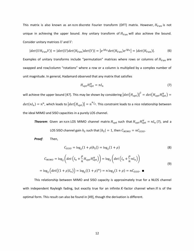
This matrix is also known as an discrete Fourier transform (DFT) matrix. However, is not

unique in achieving the upper bound. Any unitary transform of will also achieve the bound.

Consider unitary matrices and :

(6)

Examples of unitary transforms include “permutation” matrices where rows or columns of are

swapped and row/column “rotations” where a row or a column is multiplied by a complex number of

unit magnitude. In general, Hadamard observed that any matrix that satisfies

(7)

will achieve the upper bound [47]. This may be shown by considering

, which leads to . This constraint leads to a nice relationship between

the ideal MIMO and SISO capacities in a purely LOS channel.

Theorem: Given an LOS MIMO channel matrix such that (7), and a

LOS SISO channel gain such that , then .

Proof: Then,

(8)

(9)

This relationship between MIMO and SISO capacity is approximately true for a NLOS channel

with independent Rayleigh fading, but exactly true for an infinite -factor channel when is of the

optimal form. This result can also be found in [49], though the derivation is different.

13

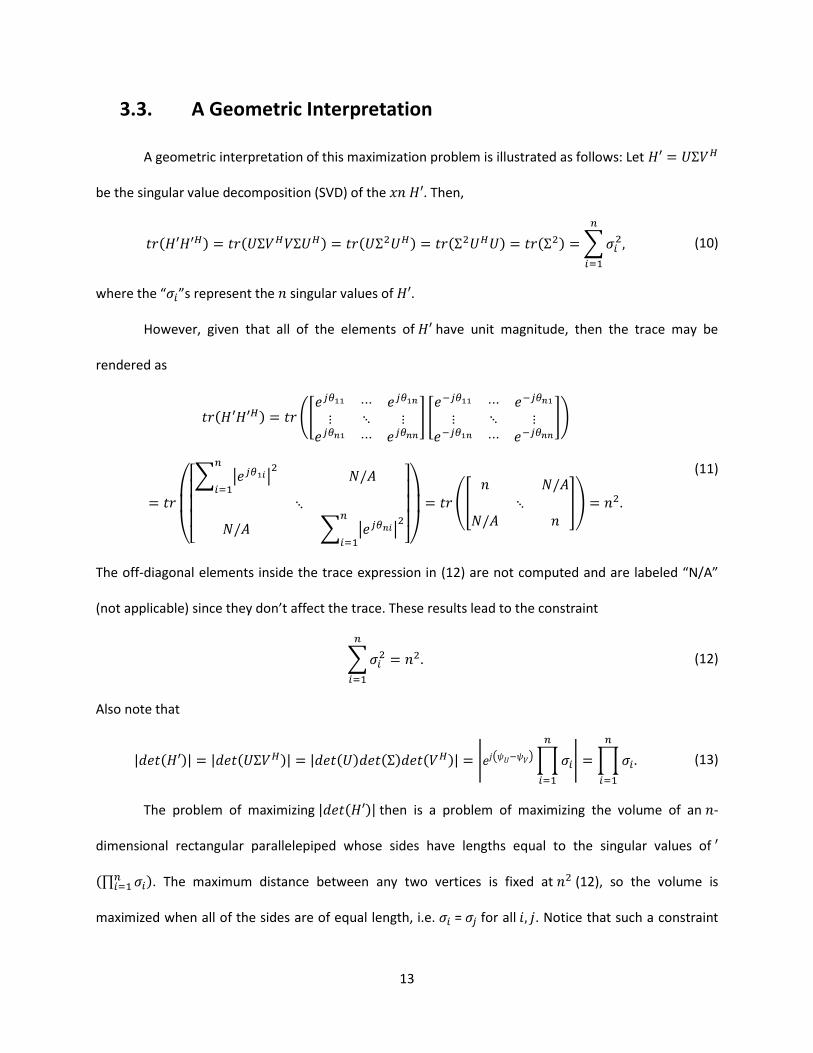
3.3. A Geometric Interpretation

A geometric interpretation of this maximization problem is illustrated as follows: Let

be the singular value decomposition (SVD) of the . Then,

(10)

where the “ ”s represent the singular values of .

However, given that all of the elements of have unit magnitude, then the trace may be

rendered as

(11)

The off-diagonal elements inside the trace expression in X(12)X are not computed and are labeled “N/A”

(not applicable) since they don’t affect the trace. These results lead to the constraint

(12)

Also note that

(13)

The problem of maximizing then is a problem of maximizing the volume of an -

dimensional rectangular parallelepiped whose sides have lengths equal to the singular values of

. The maximum distance between any two vertices is fixed at (12), so the volume is

maximized when all of the sides are of equal length, i.e. = for all . Notice that such a constraint

14

yields a condition number of unity, which has previously been demonstrated to coincide with

maximizing MIMO capacity [43].

Although the use of the determinant as a metric and the application of Hadamard’s work to

MIMO theory was derived independently, the author afterward discovered a somewhat similar analysis

done by Larsson in [49]. However, the present analysis offers a more complete discussion and different

perspective, including a comparison of the determinant with the condition number and the preceding

geometric interpretation discussion.

3.4. A 2x2 Example

Applying (5) to a 2x2 system, the ideal channel matrix has the form

(14)

Using two unitary transforms, the matrix is altered:

(15)

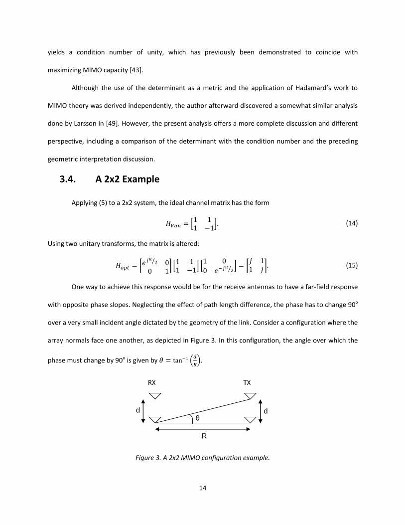
One way to achieve this response would be for the receive antennas to have a far-field response

with opposite phase slopes. Neglecting the effect of path length difference, the phase has to change 90o

over a very small incident angle dictated by the geometry of the link. Consider a configuration where the

array normals face one another, as depicted in Figure 3. In this configuration, the angle over which the

phase must change by 90o is given by .

Figure 3. A 2x2 MIMO configuration example.

d

R

θ

RX TX

d

15

This initial analysis is restricted to the configuration shown in Figure 3. In general, the link may

not yield such a favorable for a fixed and it may be useful to consider configurations for mitigating

this problem such as an array of four antennas arranged in a square where the two best antennas are

selected for transmit and receive processing.

It will also be useful to consider the capacity when such a large phase slope is not achieved, so

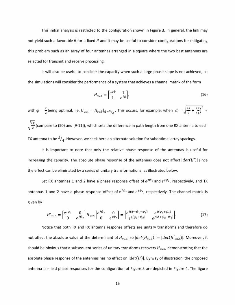
the simulations will consider the performance of a system that achieves a channel matrix of the form

(16)

with being optimal, i.e. . This occurs, for example, when

(compare to (50) and [9-11]), which sets the difference in path length from one RX antenna to each

TX antenna to be . However, we seek here an alternate solution for suboptimal array spacings.

It is important to note that only the relative phase response of the antennas is useful for

increasing the capacity. The absolute phase response of the antennas does not affect since

the effect can be eliminated by a series of unitary transformations, as illustrated below.

Let RX antennas 1 and 2 have a phase response offset of and , respectively, and TX

antennas 1 and 2 have a phase response offset of and , respectively. The channel matrix is

given by

(17)

Notice that both TX and RX antenna response offsets are unitary transforms and therefore do

not affect the absolute value of the determinant of , so . Moreover, it

should be obvious that a subsequent series of unitary transforms recovers , demonstrating that the

absolute phase response of the antennas has no effect on . By way of illustration, the proposed

antenna far-field phase responses for the configuration of Figure 3 are depicted in Figure 4. The figure

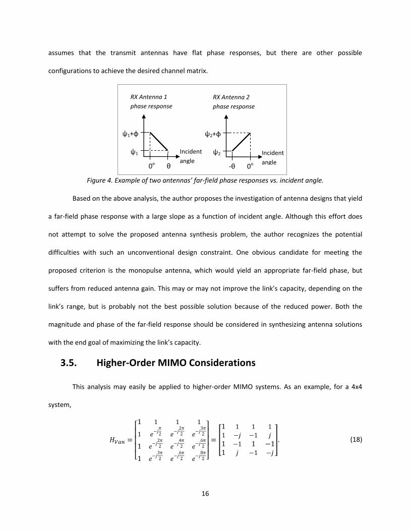
16

assumes that the transmit antennas have flat phase responses, but there are other possible

configurations to achieve the desired channel matrix.

Figure 4. Example of two antennas’ far-field phase responses vs. incident angle.

Based on the above analysis, the author proposes the investigation of antenna designs that yield

a far-field phase response with a large slope as a function of incident angle. Although this effort does

not attempt to solve the proposed antenna synthesis problem, the author recognizes the potential

difficulties with such an unconventional design constraint. One obvious candidate for meeting the

proposed criterion is the monopulse antenna, which would yield an appropriate far-field phase, but

suffers from reduced antenna gain. This may or may not improve the link’s capacity, depending on the

link’s range, but is probably not the best possible solution because of the reduced power. Both the

magnitude and phase of the far-field response should be considered in synthesizing antenna solutions

with the end goal of maximizing the link’s capacity.

3.5. Higher-Order MIMO Considerations

This analysis may easily be applied to higher-order MIMO systems. As an example, for a 4x4

system,

(18)

-θ

RX Antenna 2

phase response

ψ2+φ

ψ2

0o

Incident

angle

RX Antenna 1

phase response

ψ1+φ

ψ1

0o θ

Incident

angle

17

Note that the first row/column could be realized with a flat RX phase response; the second

row/column with an RX antenna whose phase response progresses by radians between angles

pointing to each of the TX antenna elements (we’ll call this a “phase slope” of ); the third with an

antenna with phase slope of ; and the fourth with an antenna with phase slope of or . By

employing two unitary transforms, we may redistribute the required phase responses among the

various antennas as follows:

(19)

Notice now the required phase slopes for the first through fourth rows/columns are

, respectively, where in (18) they were .

In general, the phase slopes required for an MIMO system may be written as –

,

–, …, .

3.6. Simulation Results

A simulation tool was created to compute capacities based on (1) in a Monte Carlo fashion. For a

given value of , the tool uses (4) to construct a realization of a channel matrix and creates an ensemble

of capacity values from which it can either compute an average or construct an estimate of the

complementary cumulative distribution function (CCDF) of the capacity. from (4) is of the form

given by (16) unless otherwise noted. The simulation does not take into account the contribution of path

length difference to the phase response. From previous research, it is clear that the array positions are

important in improving MIMO capacity, but the point of this analysis is to demonstrate how the phase of

the channel gains affects the capacity in order to motivate efforts to find other ways to influence those

18

phase terms. All antenna pairs are assumed to experience the same average power loss and the average

received SNR is set at 20dB.

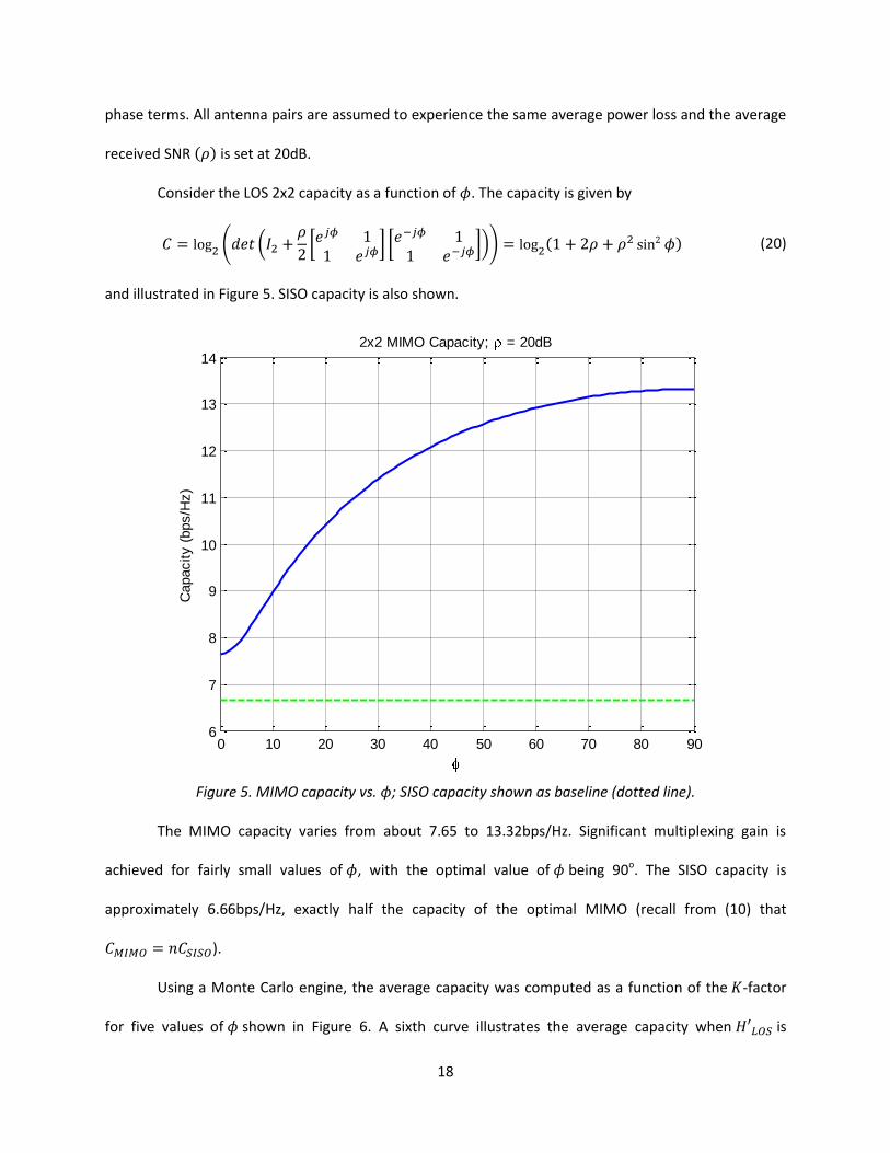
Consider the LOS 2x2 capacity as a function of . The capacity is given by

(20)

and illustrated in Figure 5. SISO capacity is also shown.

Figure 5. MIMO capacity vs. ; SISO capacity shown as baseline (dotted line).

The MIMO capacity varies from about 7.65 to 13.32bps/Hz. Significant multiplexing gain is

achieved for fairly small values of , with the optimal value of being 90o. The SISO capacity is

approximately 6.66bps/Hz, exactly half the capacity of the optimal MIMO (recall from X(10)X that

).

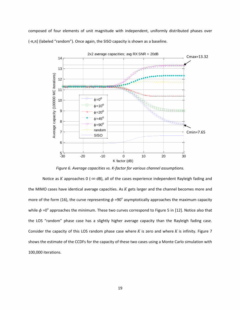
Using a Monte Carlo engine, the average capacity was computed as a function of the -factor

for five values of shown in Figure 6. A sixth curve illustrates the average capacity when is

0 10 20 30 40 50 60 70 80 906

7

8

9

10

11

12

13

14

Capacity (

bps/H

z)

2x2 MIMO Capacity; = 20dB

19

composed of four elements of unit magnitude with independent, uniformly distributed phases over

(-π,π+ (labeled “random”). Once again, the SISO capacity is shown as a baseline.

Figure 6. Average capacities vs. K-factor for various channel assumptions.

Notice as approaches 0 (- dB), all of the cases experience independent Rayleigh fading and

the MIMO cases have identical average capacities. As gets larger and the channel becomes more and

more of the form (16), the curve representing =90o asymptotically approaches the maximum capacity

while =0o approaches the minimum. These two curves correspond to Figure 5 in [12]. Notice also that

the LOS “random” phase case has a slightly higher average capacity than the Rayleigh fading case.

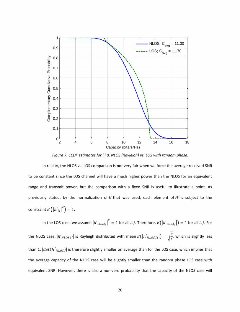
Consider the capacity of this LOS random phase case where is zero and where is infinity. Figure 7

shows the estimate of the CCDFs for the capacity of these two cases using a Monte Carlo simulation with

100,000 iterations.

-30 -20 -10 0 10 20 305

6

7

8

9

10

11

12

13

14

K factor (dB)

Avera

ge c

apacity (

100000 M

C ite

rations)

2x2 average capacities; avg RX SNR = 20dB

=0o

=10o

=20o

=45o

=90o

random

SISO

Cmax=13.32

Cmin=7.65

20

Figure 7. CCDF estimates for i.i.d. NLOS (Rayleigh) vs. LOS with random phase.

In reality, the NLOS vs. LOS comparison is not very fair when we force the average received SNR

to be constant since the LOS channel will have a much higher power than the NLOS for an equivalent

range and transmit power, but the comparison with a fixed SNR is useful to illustrate a point. As

previously stated, by the normalization of that was used, each element of is subject to the

constraint .

In the LOS case, we assume for all . Therefore, for all . For

the NLOS case, is Rayleigh distributed with mean , which is slightly less

than 1. is therefore slightly smaller on average than for the LOS case, which implies that

the average capacity of the NLOS case will be slightly smaller than the random phase LOS case with

equivalent SNR. However, there is also a non-zero probability that the capacity of the NLOS case will

2 4 6 8 10 12 14 16 180

0.1

0.2

0.3

0.4

0.5

0.6

0.7

0.8

0.9

1

Capacity (bits/s/Hz)

Com

ple

menta

ry C

um

ula

tive P

robabili

ty

NLOS; Cavg

= 11.30

LOS; Cavg

= 11.70

21

exceed the maximum capacity of the LOS case since the absolute value of each element of can

be larger than 1.

From this, we see that the MIMO multiplexing gain so evident in an independent Rayleigh fading

environment is not because of the magnitude fading since the probability distribution of the magnitude

leads to a smaller average capacity than if the RX power were fixed at its average. The multiplexing gain

instead comes from the phase of the channel matrix, which for Rayleigh fading is uniformly distributed

over (-π,π+. If a LOS channel could be made to exhibit this kind of phase distribution (our “random

phase” case), it would have a slightly higher average capacity than the NLOS channel for equivalent SNR

levels. Considering the higher power of a typical LOS channel, the capacity would be far greater. If the

phase response can be fixed to be of the form of in X(16)X instead of a random phase, the capacity

would be even higher.

22

Chapter 4: MIMO Bounds as a Function of the Determinant Metric

In Section 3.1, the authors proposed a determinant-based metric ( ) for studying LOS MIMO

capacity; was used to derive the optimal form of a LOS MIMO channel matrix. The metric is also useful

as an intuitive aid for studying capacity, an analytical tool for simulation, and may be useful for other

MIMO-related applications. This chapter presents an exploration of the relationship between this metric

( ) and the Shannon capacity by deriving upper and lower bounds of the capacity as a function of

under two different assumptions. These bounds include an 1) upper and 2) lower bound assuming a

fixed instantaneous SNR such as might be observed within a coherence time period of the channel and

3) a more detailed derivation of a previously published general lower bound. The first and second

bounds are not given in closed form for the general case, but closed form solutions are presented for

the practical case where one of the terminals, such as a mobile user, has only two antennas. The three

antenna case also has a closed form solution because it depends on the roots of a third order

polynomial, which can be given in closed form [56], but the solution was not computed for this

dissertation.

Many other papers have presented bounds on the capacity as a function of various parameters

under various assumptions. For example, researchers have explored bounds assuming Rayleigh fading

[50], Rician fading [51], Nakagami fading [52], and correlated fading [53]. Some studies assume a limited

or fixed transmit power and channel matrix Frobenius norm [54] and many others have explored bounds

for relay channels [55]. There are many more such studies, but a representative sample is presented

here. For further reading, see Zhong et al [52], which offers a good literature review and bibliography.

In Section 4.1 of this chapter, we re-introduce the determinant metric from Section 3.1 in a

more general form; in Section 4.2, the three bounds are derived; and Section 4.3 presents simulation

results.

23

4.1. A Generalized Determinant-Based Metric

The Shannon capacity of a MIMO system is given by [2]

(21)

Recall that is the received SNR, and are the number of transmit and receive antennas

respectively, is the normalized channel matrix, is the ordered singular value of , and is

defined as . Notice that maximizing the capacity (21) is nearly equivalent to maximizing

if or if , given a sufficiently large SNR. We therefore present

the general form of as

(22)

4.2. Bounding the Metric

Depending on several parameters, including , , , and the method of normalizing the

channel matrix , the relationship between and may be strongly or weakly correlated. This section

presents capacity bounds as a function of the metric under two different methods of channel matrix

normalization.

4.2.1. Fixed Instantaneous SNR

The first normalization method seems to be the most prevalent in the literature and assumes

that the instantaneous SNR for each channel realization is fixed to the value assigned to . This neglects

any fading effects and forces the receive SNR to always be a fixed value. This assumption may be useful

in cases where the SNR is estimated at the receiver and remains valid for some channel coherence time

or where the link is LOS with negligible multipath. The normalization is given by

24

(23)

Based on this normalization, we derive upper and lower bounds for the capacity (21) as a function of

(22). The general solution requires solving for the roots of an -order polynomial and a three-step

process is outlined below.

4.2.1.1. Upper Bound

To derive the upper bound, notice that . It can be easily shown that

. Therefore,

(24)

similar to (12).

Notice that and are maximized when for all . In general, the value of each

corresponds to the available capacity of the spatial subchannel. Note that can be degraded by

slowly shutting down between and of the available subchannels. To maximize for a given

value of , we shut down only subchannel. This is accomplished by setting the largest singular

values to be equal while allowing the to degrade. This is equivalent to

slowly reducing the rank of the channel matrix by 1, while keeping channel modes open for data.

With these constraints, the upper bound on the capacity can be computed by

(25)

as a function of two singular values ( and ) that are computed below.

It now remains to calculate those values as a function of and plug them into (25). To do this,

we write . Then and substituting into (24),

25

(26)

To solve for the upper bound then, we

1) solve for by finding the largest, real root of the -order polynomial whose coefficients are

given by the vector where the vector contains zeros.

Once has been found for a given , , and , we

2) solve for and

3) plug and into (25) to find the maximum capacity for a given value of .

The case

Consider a or link ( ) and define . A closed form expression of

the upper bound for the case is derived as follows.

(27)

It can be shown that with this normalization, the maximum value of is , so in this case

where , will always be real.

Solving for :

(28)

We can then solve for as follows:

26

(29)

4.2.1.2. Lower Bound

We now derive a lower bound for this normalization. Following the discussion in Section 4.2.1.1,

the smallest capacity would be realized as we shut down of the subchannels. Therefore, we set

the smallest singular values equal to one another . Notice that as

approaches zero, we slowly approach a rank-1 channel, leaving only one channel available for data

transmission. The lower bound on the capacity may then be written as

(30)

based on two singular values ( and ) that are computed as follows.

Under this assumption, we may write . Then and substituting into

(24), we write

(31)

To solve for the lower bound, we

27

1) solve for by finding the smallest, non-negative, real root of the -order polynomial whose

coefficients are given by the vector where the vector contains

zeros. Once has been found for a given , , and , we

2) solve for and

3) plug and into (30) to find the minimum capacity for a given value of .

The case

Again, consider a or link. is solved by

(32)

Solving for :

(33)

We can then solve for in closed form as follows:

(34)

which is equal to in (29). Note that with this normalization, the upper and lower bounds for a

or a are equal. In other words, when we fix the SNR of each realization to be equal, we can

28

exactly determine the capacity of a MIMO link from the determinant metric when one of the nodes has

two antennas.

Similar closed form solutions of upper and lower bounds for and can be found if the

roots of an -order polynomial can be solved in closed form. Such solutions certainly exist for

[56], but the solution is not given here.

4.2.2. Fixed Average SNR

The second normalization we consider assumes that the average receive SNR is fixed to the

value assigned to . This is accomplished by setting

(35)

as in (2). This normalization results in for all values of where is the

element of . This method allows to reflect the dynamics of a time-varying fading channel and

considers a realistic scenario with a fixed TX power. This method might be used to create an ensemble of

channel gain realizations for a given link over time.

When is composed of i.i.d. complex Gaussian random variables, the instantaneous SNR for a

given realization may be infinitely large since the Gaussian probability density functions have infinitely

long tails. Therefore, no upper bound can be found for this normalization. A lower bound result is

derived here. Upper bounds on capacity have been derived in many studies, but always with some

implicit or explicit assumption of a bounded Frobenius norm of the channel matrix. An example of a

thorough analysis with such assumptions clearly stated is found in [54]. The derivation of the lower

bound follows.

We begin by introducing the concept of majorization. We say that a vector of real numbers

weakly majorizes a second vector of real numbers ,

denoted , if , , …, , …, and . This

29

defines the concept of weak majorization. Strong majorization, denoted , may be obtained by

adding the constraint that , replacing the last inequality in the weak majorization

definition with equality.

Muirhead’s inequality [57], which is applied in the following development, states that

(36)

if and only if majorizes . Strong majorization would imply

a tighter inequality than weak majorization using Muirhead’s inequality theorem.

We now evaluate to avoid carrying the logarithm notation throughout the derivation.

(37)

which, by binomial expansion, is equivalent to

(38)

where and denotes a sum of -element products over all

permutations of base variables. In other words, if and , then

.

For the symmetric sum of (38), the vector consists of ones followed by zeros.

For a given , this vector strongly majorizes the -element vector . Therefore, by

Muirhead’s inequality,

(39)

for all values of . Substituting (39) into (38),

30

(40)

Following the chain of (37)-(40), , so

and we define the second lower bound on capacity

as

(41)

This bound is useful because it is a single closed-form expression that may be evaluated directly

as opposed to the three-step process of the bounds described earlier. The bound is also given in [50] in a

similar form, but the above is presented as a more detailed derivation and for comparison with the

bounds derived in Section 4.2.1.


We present results of i.i.d. complex Gaussian channel realizations where both (21) and (22)

are computed and compare these scatter plots to the upper and lower bounds presented above for the

two different methods of channel matrix normalization.

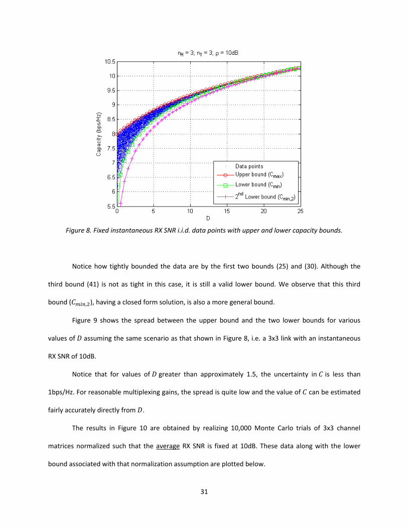
The data in Figure 8 is obtained by assuming a fixed instantaneous RX SNR of 10dB and

computing metrics for 10,000 Monte Carlo trials of a 3x3 MIMO system. The upper and lower bounds for

this normalization ( and ) are plotted along with the second lower bound in ( ).

31

Figure 8. Fixed instantaneous RX SNR i.i.d. data points with upper and lower capacity bounds.

Notice how tightly bounded the data are by the first two bounds (25) and (30). Although the

third bound (41) is not as tight in this case, it is still a valid lower bound. We observe that this third

bound ( ), having a closed form solution, is also a more general bound.

Figure 9 shows the spread between the upper bound and the two lower bounds for various

values of assuming the same scenario as that shown in Figure 8, i.e. a 3x3 link with an instantaneous

RX SNR of 10dB.

Notice that for values of greater than approximately 1.5, the uncertainty in is less than

1bps/Hz. For reasonable multiplexing gains, the spread is quite low and the value of can be estimated

fairly accurately directly from .

The results in Figure 10 are obtained by realizing 10,000 Monte Carlo trials of 3x3 channel

matrices normalized such that the average RX SNR is fixed at 10dB. These data along with the lower

bound associated with that normalization assumption are plotted below.

32

Figure 9. Capacity bound spreads for fixed instantaneous RX SNR i.i.d. realizations.

Figure 10. Fixed average RX SNR i.i.d. data points with lower capacity bound.

0 5 10 15 20 250

1

2

3

4

5

6

7

8Spread between upper and lower capacity bounds

D

Capacity (

bps/H

z)

Cmax

-Cmin

Cmax

-Cmin,2

33

In this case, as approaches zero, also approaches zero because of the potential for fading on

all channel gains, but there is still a potential for 2 channels of multiplexing when , so the spread

becomes significant for smaller values of . Notice this bound is much tighter to the data under the

assumption of a fixed average RX SNR than the same bound shown in Figure 8.

Having explored the relationship between and in this chapter, we return to the framework

outlined in Chapter 3 to explore methods for achieving the optimal form of (7) in order to achieve

higher multiplexing gain in LOS MIMO links with suboptimal array spacings.

34

Chapter 5: RACE for Fixed Point-to-Point LOS MIMO Links

Based on the results of Chapter 3, various ideas were considered for achieving the desired phase

of the channel responses. Several ideas were conceived including many designed to alter the phase

response of the MIMO antennas themselves. However, some additional analysis considering the

structure of the MIMO arrays suggested that it would be difficult, perhaps impossible, to significantly

influence the channel capacity locally without expanding the array size as other studies have suggested.

So the investigation turned to ideas by which the scattering environment could be influenced to achieve

the desired phase response of the various channel gains. This naturally led to the idea of using repeaters

strategically located to enhance the multipath [19], but in a less random fashion than a typical NLOS

environment would do. We sought to understand how we might place the repeater(s) to achieve the

optimal form of given a strongly Rician (high -factor) LOS environment with highly deterministic

channel gains. Thus, the antenna design problem is left open to the research community and we turn

our attention to the analysis of repeaters in a LOS MIMO environment.

The wireless configuration we propose to analyze initially is that of a 2x2 MIMO system with a

single repeater, shown in Figure 11. In the figure, the triangles represent antennas, the dots the centers

of the MIMO arrays, and the star a single repeater. The inter-element spacings are given by “ ” and

“ ,” the range by “ ,” and the angles the array normals make with the line connecting the centers of

the arrays are given by and . The distances between RX/TX antennas and the repeater are given

by and , respectively where is the repeater position, the

position of the RX antenna, the position of the TX antenna, , and . We

assume without loss of generality that the center of the RX array is at the origin and the center of the TX

array lies on the x-axis. We also restrict our initial analysis to two spatial dimensions and define position

vectors in the x-y plane.

35

T. .p1

pR2

pR1

RX Array TX Array

Wireless

repeater

dR dTR

R

pT1

pT2dR11

dR21 dT21

dT11

Figure 11. Wireless repeater configuration.

5.1. Channel Model

With repeaters assisting the link, the free-space channel matrix may be modeled as

the summation of channel responses:

(42)

Here, is the direct path response, is the response through the repeated path, and

is a random phase associated with the signal. The introduction of the random phase is intended to

allow for small fluctuations in node position, but the analysis will show that its value has very little

impact on the capacity when the repeater(s) are placed properly. The results presented in this chapter

correspond to the single repeater case ( ), but the models are given in their general form for later

use. We model the channel responses with the Friis transmission equation. The element of is

given by

(43)

36

depending only on the distance between the RX element and the TX element ( ) and the wave

number ( ). Similarly, the element of is given by

(44)

where and are the distances between the repeater and the TX or RX elements

respectively, and is the repeater’s power gain.

Although we primarily want to consider the effect of the repeater in a pure LOS environment,

we also need to analyze the effect of multipath fading to determine how our analysis degrades with

increasing multipath power. To account for NLOS fading, we introduce a Rician -factor similar to Error!

Reference source not found. defined as or the ratio of the power in the LOS signal to

the power in the NLOS multipath reflections arriving at the receiver. We model the NLOS portion

as a complex Gaussian random variable with zero mean and unit variance. Thus, the final

channel matrix is given by

(45)

5.2. Repeater Model

For this analysis, we assume a repeater with sufficient isolation and gain to overcome the path

loss from any location while maintaining stability. Later, we will determine the required gain for the

proposed scenario and determine whether this assumption is valid by considering experimental isolation

values. In the future, it would be prudent to incorporate a more realistic model for isolation, but the

present analysis should serve to demonstrate the feasibility of the concept.

The repeater model incorporates noise amplification [42] and the effect of colored noise as

follows. Following the model in [33], the autocorrelation matrix of the noise power at the RX is given by

37

(46)

where denotes the channel response of the -repeater-to-RX path , is the

gain of the repeater, is the noise power introduced by the RX, and is the

noise power introduced by the repeater. Here, is Boltzmann’s constant, and are the system

noise temperatures of the RX and repeater respectively, and is the signal bandwidth, which we

assume to be 20MHz. The noise figure of each system is assumed to be 3dB. The noise temperature ( )

is calculated from the noise figure ( ) by , where is room temperature, assumed to

be 290oK.

The optimal gain of the repeater is given by to ensure that the power levels

the RX sees from the direct and repeated paths are equal. Here is the distance from the center of

the RX array to the repeater, is the distance from the center of the TX array to the repeater,

and is the range.

The normalized noise autocorrelation from (46) is then decomposed as , where

contains the eigenvectors of and is a diagonal matrix of the eigenvalues. To calculate the

capacity, the noise must be whitened by applying . The resultant noise power after

whitening is equal to . The channel matrix to be used in computing the capacity using the colored

noise model is given by . An ideal repeater is modeled by using instead of . Some results

from the ideal model are shown for comparison and to more clearly illustrate trends.

5.3. 2x2 Repeater Position Analysis

Two metrics will be considered in analyzing the impact of the repeater as a function of position

and a third metric is derived in Section 5.4 to give an intuitive feel for optimal positions and introduce a

38

simple system deployment methodology. The first metric is Shannon’s capacity [1] given for MIMO

systems [2] as

(47)

or

(48)

where is the ideal capacity, the colored capacity, is the transmit power and is the noise

power introduced by the receiver (compare to (1)). The transmit power is fixed to ensure a

predetermined average baseline SNR ( ) by where represents the path loss

for the direct path (TX to RX) modeled by the Friis transmission equation. Thus represents the average

SNR the RX would see without repeaters. With the repeater(s) assisting, the actual SNR will be

somewhat larger.

The second metric ( ) is derived from the capacity by assuming a sufficiently large SNR [18] as

discussed in Section 4.1, and is given by (22) where is normalized by

(49)

This determinant metric ( ) is equal to the square of the product of the singular values of , so when

any one singular value is close to zero, the metric is close to zero. This would indicate at least one

degenerate sub-channel (i.e., less than full multiplexing gain capacity). Therefore, when the capacity

improves from a boost in SNR or the use of more antennas on one side or the other of the link, the

determinant should remain largely unaffected, assuming the channel rank is limited by the environment

to less than full rank. This makes it a useful metric in terms of achieving the full multiplexing gain, which

we seek to do here. We also use it to highlight the utility of a proposed positioning metric in Section 5.4.

39

5.3.1. Optimal Inter-Element Spacing

Assuming TX and RX have the same inter-element spacing, the optimal spacing for a 2x2 MIMO

system is given by [9-11]

(50)

For the repeater concept to be useful, we must ensure that we are operating beyond the optimal range

for our given spacing or, equivalently, we must make sure that the antenna spacing is less than the

optimal spacing for our given range.

5.3.2. Free Space Repeater Positioning

For our analysis, we use a carrier frequency of 2.4 GHz, so λ = 0.125m. Let = = 0 so that

the array normals lie on the x-axis. Let the range R = 900m (2953ft.) and the antenna spacings = =

0.75m (2.46ft) = 6λ. The SNR is set to 20dB. For brevity in the rest of the analysis, we will keep these

parameters constant (see Table 1) unless otherwise noted.

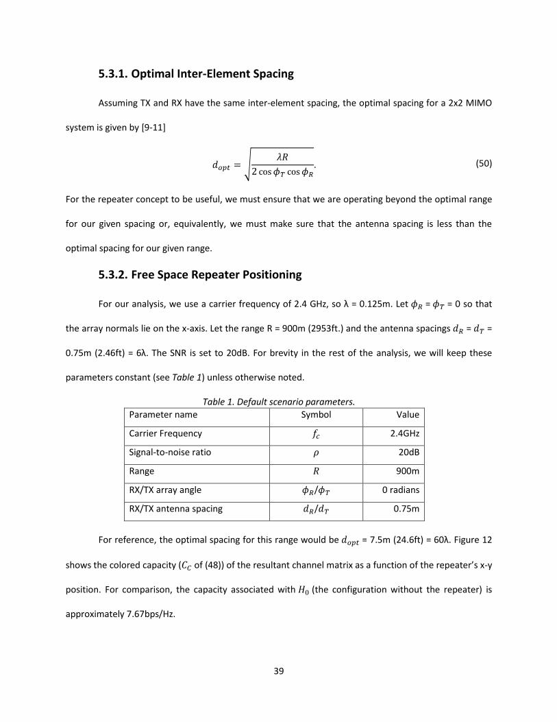
Table 1. Default scenario parameters.

Parameter name Symbol Value

Carrier Frequency 2.4GHz

Signal-to-noise ratio 20dB

Range 900m

RX/TX array angle / 0 radians

RX/TX antenna spacing / 0.75m

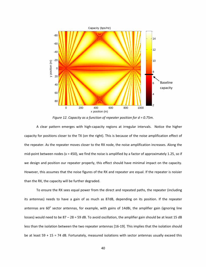
For reference, the optimal spacing for this range would be = 7.5m (24.6ft) = 60λ. Figure 12

shows the colored capacity ( of (48)) of the resultant channel matrix as a function of the repeater’s x-y

position. For comparison, the capacity associated with (the configuration without the repeater) is

approximately 7.67bps/Hz.

40

Figure 12. Capacity as a function of repeater position for d = 0.75m.

A clear pattern emerges with high-capacity regions at irregular intervals. Notice the higher

capacity for positions closer to the TX (on the right). This is because of the noise amplification effect of

the repeater. As the repeater moves closer to the RX node, the noise amplification increases. Along the

mid-point between nodes (x = 450), we find the noise is amplified by a factor of approximately 1.25, so if

we design and position our repeater properly, this effect should have minimal impact on the capacity.

However, this assumes that the noise figures of the RX and repeater are equal. If the repeater is noisier

than the RX, the capacity will be further degraded.

To ensure the RX sees equal power from the direct and repeated paths, the repeater (including

its antennas) needs to have a gain of as much as 87dB, depending on its position. If the repeater

antennas are 60o sector antennas, for example, with gains of 14dBi, the amplifier gain (ignoring line

losses) would need to be 87 – 28 = 59 dB. To avoid oscillation, the amplifier gain should be at least 15 dB

less than the isolation between the two repeater antennas [16X-X19X]. This implies that the isolation should

be at least 59 + 15 = 74 dB. Fortunately, measured isolations with sector antennas usually exceed this

x position (m)

y p

ositio

n (

m)

Capacity (bps/Hz)

0 200 400 600 800 1000

-80

-60

-40

-20

0

20

40

60

80

2

4

6

8

10

12

14

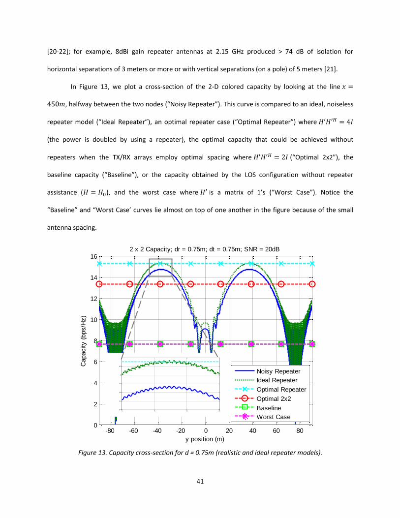
Baseline

capacity

41

[20-22]; for example, 8dBi gain repeater antennas at 2.15 GHz produced > 74 dB of isolation for

horizontal separations of 3 meters or more or with vertical separations (on a pole) of 5 meters [21].

In Figure 13, we plot a cross-section of the 2-D colored capacity by looking at the line

, halfway between the two nodes (“Noisy Repeater”). This curve is compared to an ideal, noiseless

repeater model (“Ideal Repeater”), an optimal repeater case (“Optimal Repeater”) where

(the power is doubled by using a repeater), the optimal capacity that could be achieved without

repeaters when the TX/RX arrays employ optimal spacing where (“Optimal 2x2”), the

baseline capacity (“Baseline”), or the capacity obtained by the LOS configuration without repeater

assistance ( ), and the worst case where is a matrix of 1’s (“Worst Case”). Notice the

“Baseline” and “Worst Case’ curves lie almost on top of one another in the figure because of the small

antenna spacing.

Figure 13. Capacity cross-section for d = 0.75m (realistic and ideal repeater models).

-80 -60 -40 -20 0 20 40 60 800

2

4

6

8

10

12

14

16

y position (m)

Capacity (

bps/H

z)

2 x 2 Capacity; dr = 0.75m; dt = 0.75m; SNR = 20dB

Noisy Repeater

Ideal Repeater

Optimal Repeater

Optimal 2x2

Baseline

Worst Case

-45 -40 -35 -3014.2

14.4

14.6

14.8

15

15.2

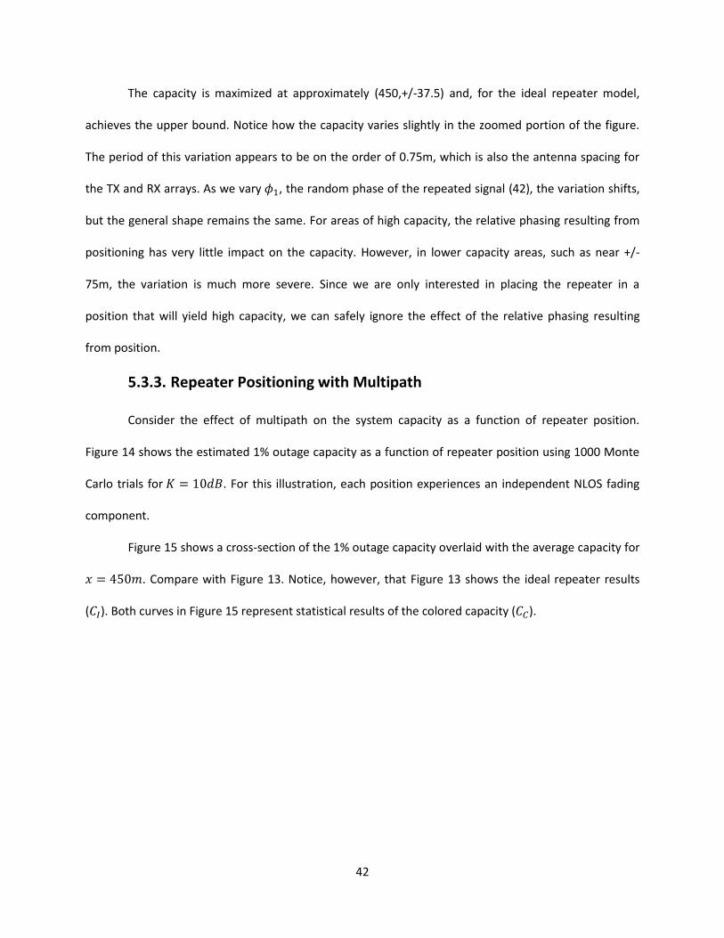
42

The capacity is maximized at approximately (450,+/-37.5) and, for the ideal repeater model,

achieves the upper bound. Notice how the capacity varies slightly in the zoomed portion of the figure.

The period of this variation appears to be on the order of 0.75m, which is also the antenna spacing for

the TX and RX arrays. As we vary , the random phase of the repeated signal (42), the variation shifts,

but the general shape remains the same. For areas of high capacity, the relative phasing resulting from

positioning has very little impact on the capacity. However, in lower capacity areas, such as near +/-

75m, the variation is much more severe. Since we are only interested in placing the repeater in a

position that will yield high capacity, we can safely ignore the effect of the relative phasing resulting

from position.

5.3.3. Repeater Positioning with Multipath

Consider the effect of multipath on the system capacity as a function of repeater position.

Figure 14 shows the estimated 1% outage capacity as a function of repeater position using 1000 Monte

Carlo trials for . For this illustration, each position experiences an independent NLOS fading

component.

Figure 15 shows a cross-section of the 1% outage capacity overlaid with the average capacity for

. Compare with Figure 13. Notice, however, that Figure 13 shows the ideal repeater results

( ). Both curves in Figure 15 represent statistical results of the colored capacity ( ).

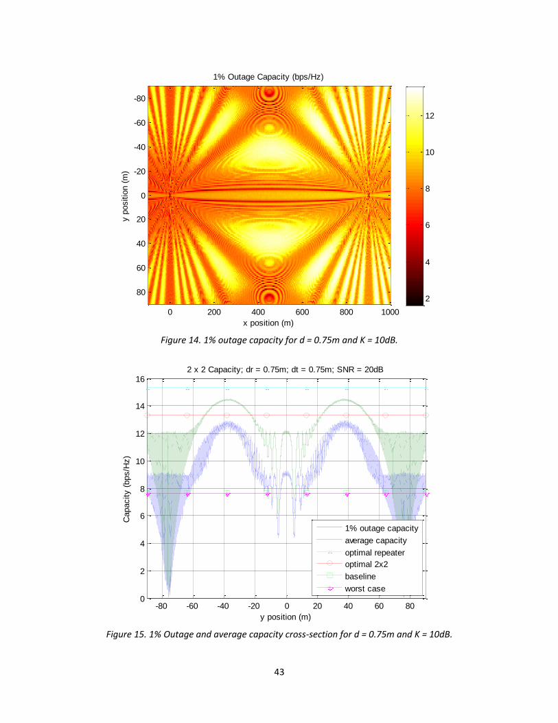
43

Figure 14. 1% outage capacity for d = 0.75m and K = 10dB.

Figure 15. 1% Outage and average capacity cross-section for d = 0.75m and K = 10dB.

x position (m)

y p

ositio

n (

m)

1% Outage Capacity (bps/Hz)

0 200 400 600 800 1000

-80

-60

-40

-20

0

20

40

60

802

4

6

8

10

12

-80 -60 -40 -20 0 20 40 60 800

2

4

6

8

10

12

14

16

y position (m)

Capacity (

bps/H

z)


1% outage capacity

average capacity

optimal repeater

optimal 2x2

baseline

worst case

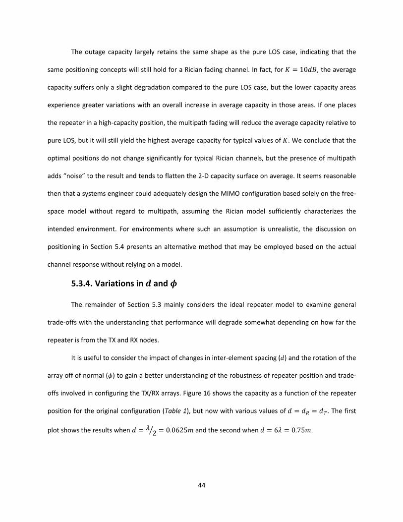
44

The outage capacity largely retains the same shape as the pure LOS case, indicating that the

same positioning concepts will still hold for a Rician fading channel. In fact, for , the average

capacity suffers only a slight degradation compared to the pure LOS case, but the lower capacity areas

experience greater variations with an overall increase in average capacity in those areas. If one places

the repeater in a high-capacity position, the multipath fading will reduce the average capacity relative to

pure LOS, but it will still yield the highest average capacity for typical values of . We conclude that the

optimal positions do not change significantly for typical Rician channels, but the presence of multipath

adds “noise” to the result and tends to flatten the 2-D capacity surface on average. It seems reasonable

then that a systems engineer could adequately design the MIMO configuration based solely on the free-

space model without regard to multipath, assuming the Rician model sufficiently characterizes the

intended environment. For environments where such an assumption is unrealistic, the discussion on

positioning in Section 5.4 presents an alternative method that may be employed based on the actual

channel response without relying on a model.

5.3.4. Variations in and

The remainder of Section 5.3 mainly considers the ideal repeater model to examine general

trade-offs with the understanding that performance will degrade somewhat depending on how far the

repeater is from the TX and RX nodes.

It is useful to consider the impact of changes in inter-element spacing ( ) and the rotation of the

array off of normal ( ) to gain a better understanding of the robustness of repeater position and trade-

offs involved in configuring the TX/RX arrays. Figure 16 shows the capacity as a function of the repeater

position for the original configuration (Table 1), but now with various values of . The first

plot shows the results when and the second when .

45

a) d = 0.0625m (λ/2) b) d = 0.75m (6λ)

Figure 16. Capacity vs. repeater position for various inter-element spacings (d).

We conclude that larger values of allow the optimal position regions to come closer to the

arrays, but they also decrease in size, indicating a design trade-off between robustness in position and

repeater requirements (specifically, isolation, gain, and noise figure) because of longer path distances.

Longer distances also increase the delay spread introduced by the repeater.

The same is true for smaller values of . We have thus far considered only the case when the

arrays face one another ( ). When one or both of the arrays are rotated by radians,

assuming free-space propagation without a repeater, the channel rank is always equal to one. By using a

repeater, however, the optimal capacity can be achieved, but the optimal position regions become

larger and farther away than when is smaller. The same trade-offs exist here between position

robustness and repeater and delay spread requirements, as shown in the following analysis.

Consider the capacity vs. repeater position plots in Figure 17 using the default parameters

(Table 1) with various angles of array rotations. The first plot shows the results when ,

while the second plot shows the results for . The figure also shows a simple diagram

representing the array configurations for each subplot.

x position (m)

y p

ositio

n (

m)

Ideal Repeater Capacity (bps/Hz)

0 200 400 600 800 1000

-800

-600

-400

-200

0

200

400

600

800

4

6

8

10

12

14

x position (m)

y p

ositio

n (

m)


0 200 400 600 800 1000

-800

-600

-400

-200

0

200

400

600

800 2

4

6

8

10

12

14

46

a) b)

Figure 17. Capacity vs. repeater position for various angles of array rotation.

For small values of and large values of , assuming we bound the orientation by ,

we find large areas of optimal repeater placement at large distances from the TX/RX nodes. This leads to

more robust positioning requirements at the expense of longer path lengths. The longer path lengths

lead to stricter requirements on repeater isolation and gain and potential introduction of increased

noise amplification and delay spread. For large values of and small values of , path lengths may be

shortened at the expense of reduced positioning robustness.

5.3.5. Three-Dimensional Repeater Positioning Analysis

Some simple analysis has been done in 3 dimensions by expanding the simulation to incorporate

the z-axis. The following shows capacity vs. position for various z-planes. Figure 18 shows the capacity

for the z = 0m, z = 100m, and z = 1000m planes.

x position (m)

y p

ositio

n (

m)


0 200 400 600 800 1000

-300

-200

-100

0

100

200

300

2

4

6

8

10

12

14

x position (m)

y p

ositio

n (

m)


0 200 400 600 800 1000

-300

-200

-100

0

100

200

300

2

4

6

8

10

12

14

47

a) b)

c)

Figure 18. Capacity vs. repeater position for various elevations.

We conclude from this preliminary analysis that repeater position robustness may be affected

by the height of the repeater. This is an area for possible future research to examine trade-offs in TX/RX

antenna beam patterns, capacity, and positioning robustness in three dimensions. For example, it is

worth considering the relative capacity for a link where antennas are constructed to direct energy

between TX and RX nodes versus antennas with multiple beams to include the repeater location(s) to

enhance the MIMO multiplexing gain. Potential platforms for elevating the repeater may include towers,

blimps, UAVs or other aircraft, and possibly satellite.

x position (m)

y p

ositio

n (

m)


0 200 400 600 800 1000

-80

-60

-40

-20

0

20

40

60

80

2

4

6

8

10

12

14

x position (m)

y p

ositio

n (

m)


0 200 400 600 800 1000

-80

-60

-40

-20

0

20

40

60

80

2

4

6

8

10

12

14

x position (m)

y p

ositio

n (

m)


0 200 400 600 800 1000

-80

-60

-40

-20

0

20

40

60

80

2

4

6

8

10

12

14

48

5.4. A 2x2 Repeater Position Metric

The following analysis serves to explain the shape of the capacity surface as a function of

repeater position for a 2x2 link and proposes a metric to be used in designing such a system.

To provide insight into the general 2x2 solution, consider the special case of ,

which yields the normalized, approximate free-space channel matrix for the long-distance

link without the repeater. In this case, we see that by adding the repeated channel response matrix

, we create the full-rank matrix . represents the desired

repeater contribution and can be written as , where is the normalized

array response for both the TX and RX arrays to a point source at the desired repeater location. We

observe that this point source would be in a null of the array patterns for the TX and RX arrays,

respectively, if unity beamformer weights were applied to each array.

In the case of non-zero and , , where

and denotes the transpose operator.

To make full rank such that , the desired repeated path response

should be . If we apply a weight vector to the RX beamformer

to steer the main beam in the direction of the TX array, the array response in the

direction of the ideally positioned repeater will be . In other words, the

repeater will be in a null of the RX array response when the array’s main beam is steered toward the TX.

A similar analysis shows that the ideal repeater position is in a null of the TX array response when the

array’s main beam is steered toward the RX.

So, to maximize the MIMO capacity, the repeater should be located in the nulls of both of these

imaginary beamformers when their beams are steered toward one another. This offers a metric for

determining the optimal locations and also suggests a method for designing such a system. Supposing

49

we have flexibility in the placement of our repeater, we can fix the TX and RX antennas and find the

position where the power received from either one of these beamformers is minimal when the power

coupled between them is maximized by beam steering. If we don’t have such flexibility, we may position

the MIMO antennas with appropriate phase shifting until we see a notch in the power at the repeater.

Let

(51)

be a 2x2 null-space positioning metric, where and are the RX and TX array responses in the

direction of a potential repeater position when the main beam of each array is steered in the direction

of the other. Figure 19a plots this metric as a function of repeater position for the standard

configuration defined for this analysis (Table 1). Compare this result to the plot of the determinant

metric (22) for the same configuration, shown in Figure 19b. Obviously, the null-space metric has

no mechanism for computing the effect of noise coloring and amplification introduced by the repeater.

Consequently, this is a more accurate measure of an ideal repeater’s effect, but can be used to

approximately analyze and predict performance.

a) Positioning metric (yNS) b) Determinant metric X(25)

Figure 19. Null-Space and Determinant metrics as a function of repeater position for d = 0.75m.

Based on the assumptions used to derive , the utility of the metric will degrade as the

antenna spacing approaches the optimal. However, the impact of the repeater becomes less significant

x position (m)

y p

ositio

n (

m)

yNS

= (2-|yR|)(2-|y

T|)

0 200 400 600 800 1000

-80

-60

-40

-20

0

20

40

60

80

0.5

1

1.5

2

2.5

3

3.5

x position (m)

y p

ositio

n (

m)

det(H'H'H)

0 200 400 600 800 1000

-80

-60

-40

-20

0

20

40

60

80

2

4

6

8

10

12

14

16

50

as the spacing increases, so we typically want to consider spacings that are much smaller than the

optimal. For the range of 900m, it works very well at least up to 3.75m, or half the optimal spacing.

5.5. Repeater Power and Delay Spread

A brief investigation on the impact of the repeater’s gain is conducted here. We consider the

impact of the power the RX sees from the direct path relative to the power it sees from the repeated

path. We also consider the delay spread introduced by the repeater as a function of the repeater’s

position.

5.5.1. Repeater Power Analysis

Let (twice the previous distance) and set the repeater location to (450,19),

which is one of the higher capacity positions for that spacing. The spacing was increased to highlight the

difference between the “baseline” and “worst case” curves in Figure 20, which shows the MIMO

capacity as a function of the repeated-to-direct path power ratio using both the realistic and ideal

repeater models. Here, the final channel matrix for each power level has been normalized as

. Notice that this normalization is different than the one used in (49) and the capacity will be

somewhat lower. We utilize this normalization to allow for a simple comparison of MIMO multiplexing

gain without accounting for the impact of the increased SNR because of the repeater and to illustrate

trends that are not observable with the previous normalization.

Optimal capacity is achieved when the receiver sees equal power from both sources. If we

consider the repeated signal as a multipath reflection, this would be equivalent to reducing the -factor

to a value of one. As the repeater power decreases from this optimal point, the ideal model results

approach the baseline capacity. As the repeater power becomes the dominant signal, the ideal results

approach the worst case capacity.

51

Figure 20. Capacity as a function of repeated-to-direct path power ratio for d=1.5m.

5.5.2. Delay Spread Analysis

Because the optimal repeater positions usually require a longer repeated signal path than the

direct signal path, it is important to consider the delay spread induced by the use of the repeater at

various locations and ensure that a typical system can function with such a delay spread. For the

repeater positions previously simulated, the delay spread varies from 0 to approximately 796ns.

Obviously, the utility of this concept will depend on the system. By way of example, Table 2

illustrates the delay spread tolerances for various bandwidths and cyclic prefix lengths of a typical

WiMax system based on the 802.16 standard [58], assuming an OFDM symbol length of 256 samples.

Table 2. Delay spread tolerances for various bandwidths and cyclic prefix lengths.

3.5 MHz 5 MHz 20 MHz

1/16 (16 bits) 4μs 2.8μs 694ns

1/8 (32 bits) 8μs 5.6μs 1.4μs

1/4 (64 bits) 12μs 11.1μs 2.8μs

-40 -30 -20 -10 0 10 20 30 407

8

9

10

11

12

13

14

A12/A

02 (dB)

Capacity (

bps/H

z)


Repeater

Ideal Repeater

optimal 2x2

baseline

worst case

52

For the configuration considered, the delay spread introduced by the repeater should not

present a problem for a typical WiMax system. As the range increases, antenna spacing decreases, or

repeater placement options are limited geographically, delay spread could become an issue and should

be considered in determining repeater placement for a system deployment.

5.6. Discussion

It has been observed in this chapter that LOS MIMO multiplexing gain may be improved by the

use of a single wireless on-frequency repeater, if the repeater is positioned properly. For smaller

antenna spacings, the areas of optimal position are larger, offering robustness in placement, but also

farther away from the MIMO arrays, requiring more repeater gain and isolation for the same range. The

RACE concept may be useful in long-range LOS links such as building-top or tower-mounted microwave

links. Cellular backhaul and high-speed wireless bridges are two potential candidates.

We note that the repeater’s power is a concern and must be considered in a system

deployment. In a static configuration, the repeater gain should be carefully calibrated to ensure the

direct and repeated signals have nearly equal power at the receiver. In a mobile configuration or in

other scenarios where the channel’s impact on power coupling varies significantly, this limitation could

potentially be overcome by 1) feedback from the receiver to enable the repeater to adapt its gain or 2)

multiple repeaters with sufficient gain to overwhelm the TX/RX LOS signal. The first option requires a

smarter repeater than we have discussed while the second option might be considered wasteful of

resources.

In the next chapter, we consider higher-order MIMO links and analyze the utility of RACE for

maximizing MIMO multiplexing gain when the link is assisted by multiple repeaters.

53

Chapter 6: Higher Order MIMO

6.1. Introduction

Extending the Null-Space analysis from Section 5.4, this chapter [59] presents a theoretical

analysis of the impact of positioning on achievable multiplexing gain in LOS environments for the

general case using repeaters where . Considering the steering vectors pointing

toward the various repeaters, the analysis shows that full multiplexing may be achieved by ensuring

mutually orthogonal steering vectors from the perspective of both arrays pointing toward the opposite

array and toward each repeater. This analysis may potentially aid in network deployment and relaying

strategies, configuring MIMO-enabled point-to-point microwave links, and potentially enabling MIMO

for LOS cellular channels. The results may also be useful in understanding the impact of scattering

environments on available MIMO capacity.

A conceptual system diagram of the RACE concept applied to a 4x4 MIMO system with 3 single-

antenna wireless repeaters is shown in Figure 21. In the figure, triangles represent MIMO antenna

elements, stars represent repeaters, and dashed lines represent LOS channel coupling. These lines have

been drawn to illustrate the LOS channel response and a single repeater path response. The other two

repeaters also contribute to the channel response, but these channel couplings have not been

illustrated.

In Section 6.2, we present five sufficient conditions for achieving full MIMO multiplexing with

wireless repeaters; Section 6.3 describes the channel model; and Section 6.4 presents a proof of the

sufficiency of the conditions in Section 6.2. In Section 6.5, we offer simulation results from a 4x4 MIMO

system to illustrate the RACE concept; we explore trade-offs associated with suboptimally-placed

repeaters in Section 6.6; and discuss conclusions in Section 6.7.

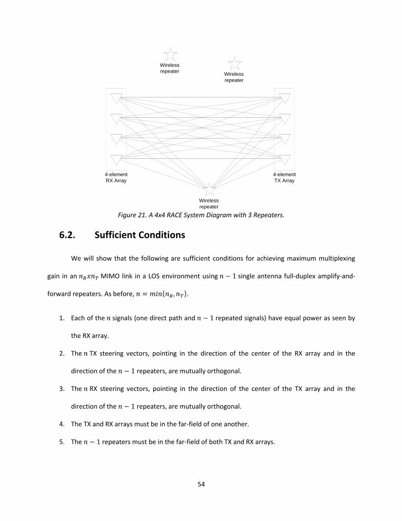
54

4-element

RX Array

4-element

TX Array

Wireless

repeater

Wireless

repeaterWireless

repeater

Figure 21. A 4x4 RACE System Diagram with 3 Repeaters.

6.2. Sufficient Conditions

We will show that the following are sufficient conditions for achieving maximum multiplexing

gain in an MIMO link in a LOS environment using single antenna full-duplex amplify-and-

forward repeaters. As before, .

1. Each of the signals (one direct path and repeated signals) have equal power as seen by

the RX array.

2. The TX steering vectors, pointing in the direction of the center of the RX array and in the

direction of the repeaters, are mutually orthogonal.

3. The RX steering vectors, pointing in the direction of the center of the TX array and in the

direction of the repeaters, are mutually orthogonal.

4. The TX and RX arrays must be in the far-field of one another.

5. The repeaters must be in the far-field of both TX and RX arrays.

55

By a simple extension of the results in Sections 3.2-3.3, we note that if , multiplexing

gain is considered to be maximized if (7) for some positive, real-valued . Likewise, if

, the multiplexing gain is maximized if .

6.3. Approximate Channel Model

The exact channel model presented in Section 5.1 is used in the simulation tool to generate the

results shown in Section 6.5; however, an approximate channel model is presented here as a means to

proving the sufficiency of the conditions presented above. Consider an MIMO link in a LOS

configuration where the RX node has antennas and the TX node has antennas. Applying condition

#4 from Section 6.2, we assume that each node is in the far field of the other array (the range is large

relative to the array size), so we may approximate the LOS channel response of the direct path without

multipath as an outer product of two steering vectors:

(52)

where is the RX steering vector in the direction of the center of the TX array, is the TX steering

vector in the direction of the center of the RX array, is a positive, real-valued variable representing

the path loss of the direct path, and is a phase term to account for fractional wavelength distances.

This phase term is necessary to construct actual channel gains because the steering vector accounts for

direction only and is blind to range, but the phase term disappears in the analysis, so we do not

compute its value. The steering vectors are given by [60]

(53)

where is the wave number vector pointing from the center of the RX array to the center of the TX

array, is the wave number vector pointing from the center of the TX array to the center of the RX

56

array, is the vector from the center of the RX array to the RX antenna, and is the vector

from the center of the TX array to the TX antenna. From [60], we note that the norm of any wave

number vector is given by where is the wavelength of the carrier.

Assuming the repeaters are in the far-field of both TX and RX arrays (condition #5 from

Section 6.2), we may similarly approximate the channel response of the path through the repeater

as

(54)

where is the RX steering vector in the direction of the repeater, is the TX steering vector in

the direction of the repeater, is a positive, real-valued variable representing the path loss of the

path through the repeater (including loss from two paths and the gain of the repeater), and is a

phase term to account for fractional wavelength distances.

The composite LOS channel response may then be approximated as the sum of the channel

responses of the various paths,

(55)

6.4. Sufficiency Proof

Having applied the fourth and fifth conditions from Section 6.2 to construct an approximate

channel model, we now apply the first three conditions, which we rewrite as follows based on the

parameter definitions above:

1. for all

2.

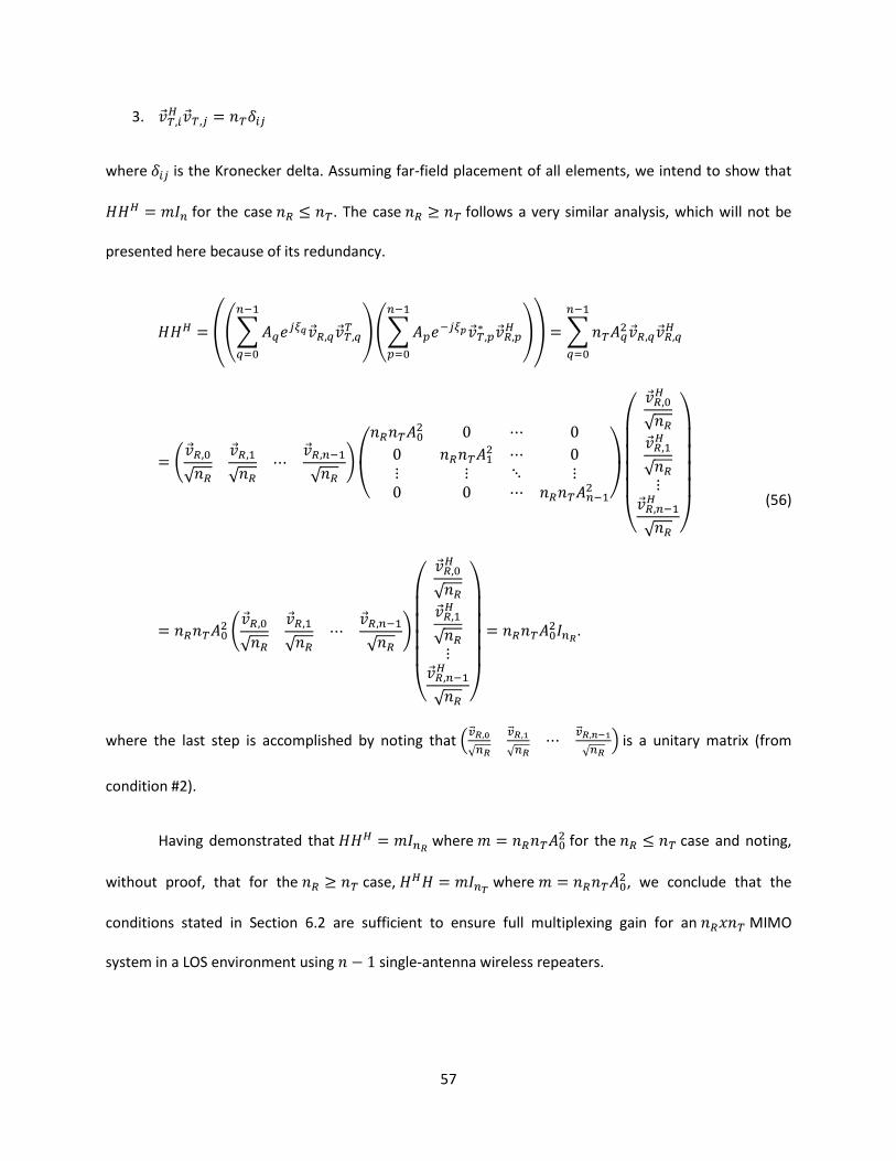
57

3.

where is the Kronecker delta. Assuming far-field placement of all elements, we intend to show that

for the case . The case follows a very similar analysis, which will not be

presented here because of its redundancy.

(56)

where the last step is accomplished by noting that is a unitary matrix (from

condition #2).

Having demonstrated that where for the case and noting,

without proof, that for the case, where , we conclude that the

conditions stated in Section 6.2 are sufficient to ensure full multiplexing gain for an MIMO

system in a LOS environment using single-antenna wireless repeaters.

58

6.5. A 4x4 Example

Having demonstrated certain conditions as sufficient for achieving full MIMO multiplexing using

wireless repeaters, we present an example of achieving full multiplexing (approximately four

times the baseline capacity, that is, the capacity without repeater assistance) with a 4x4 MIMO system

assisted by three strategically placed single-antenna wireless repeaters. For the simulations, we use the

channel model of (42) described in Section 5.1 and the amplify-and-forward repeater model of Section

5.2 with results for both noiseless and noisy repeaters incorporating the effects of noise coloring and

amplification. For the results presented here, we assume a carrier frequency of 2.4GHz, a range of

900m, an inter-element spacing of 0.75m (for a total TX/RX array length of 2.25m), and a baseline SNR

of 20dB. Figure 22a shows the capacity of the system (47) with a single noiseless repeater as a function

of the position of that repeater. We also assume the TX/RX nodes and repeaters are in the x-y plane and

define positions in two dimensions.

Figure 22b shows the results of a generalized null-space positioning metric ( ):

(57)

where is the number of wireless repeaters. This metric gives additional insight and offers a practical

methodology for ideal placement of the repeaters. Notice that the metric is maximized when the TX

and RX steering vectors are mutually orthogonal, which satisfies conditions two and three of Section 6.2.

A more complete development of a similar metric is given in Section 7.3.

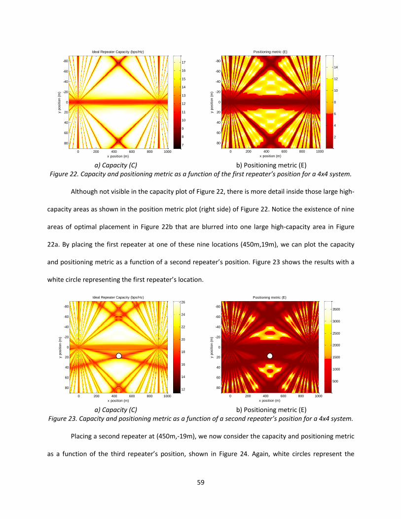
59

a) Capacity (C) b) Positioning metric (E)

Figure 22. Capacity and positioning metric as a function of the first repeater’s position for a 4x4 system.

Although not visible in the capacity plot of Figure 22, there is more detail inside those large high-

capacity areas as shown in the position metric plot (right side) of Figure 22. Notice the existence of nine

areas of optimal placement in Figure 22b that are blurred into one large high-capacity area in Figure

22a. By placing the first repeater at one of these nine locations (450m,19m), we can plot the capacity

and positioning metric as a function of a second repeater’s position. Figure 23 shows the results with a

white circle representing the first repeater’s location.


Figure 23. Capacity and positioning metric as a function of a second repeater’s position for a 4x4 system.

Placing a second repeater at (450m,-19m), we now consider the capacity and positioning metric

as a function of the third repeater’s position, shown in Figure 24. Again, white circles represent the

x position (m)

y p

ositio

n (

m)


0 200 400 600 800 1000

-80

-60

-40

-20

0

20

40

60

807

8

9

10

11

12

13

14

15

16

17

x position (m)

y p

ositio

n (

m)

Positioning metric (E)

0 200 400 600 800 1000

-80

-60

-40

-20

0

20

40

60

80

2

4

6

8

10

12

14

x position (m)

y p

ositio

n (

m)


0 200 400 600 800 1000

-80

-60

-40

-20

0

20

40

60

80 12

14

16

18

20

22

24

26

x position (m)

y p

ositio

n (

m)


0 200 400 600 800 1000

-80

-60

-40

-20

0

20

40

60

80

500

1000

1500

2000

2500

3000

3500

60

positions of the first two repeaters. We observe that the options for repeater placement diminish with

each successive placement.


Figure 24. Capacity and positioning metric as a function of the third repeater’s position for a 4x4 system.

Figure 25 shows a plot of the cross-section of 1) the ideal capacity of Figure 24a (“Ideal

Repeater”) and 2) the capacity using a noisy repeater accounting for repeater-induced noise coloring

and amplification (“Noisy Repeater”). Also shown in the figure are 3) the optimal capacity using 3

repeaters (“Optimal Repeater”), 4) the optimal capacity that could be achieved without repeaters when

the TX/RX arrays employ proper spacing (“Optimal 4x4”), 5) the baseline capacity, or the capacity

obtained by the LOS configuration without repeater assistance (“Baseline”), and 6) the worst case

capacity when the channel matrix is a matrix of ones (“Worst Case”). The “Optimal Repeater” curve is

higher than the “Optimal 4x4” curve simply because of the increase in SNR because of the presence of

the repeaters. The baseline SNR is 20dB, but with three repeaters, the actual SNR is closer to 26dB.

Placing the third repeater at (450m,38m) will yield an optimal capacity (34.6 bps/Hz) for the

ideal repeater model and for a realistic model, about 31.6 bps/Hz. This 9% degradation in capacity is the

result of noise amplification and coloring introduced by the three repeaters. Table 3 shows the

capacities associated with the various curves when three repeaters are placed at (450m,19m), (450m,-

19m), and (450m,38m).

x position (m)

y p

ositio

n (

m)


0 200 400 600 800 1000

-80

-60

-40

-20

0

20

40

60

8020

22

24

26

28

30

32

34

x position (m)

y p

ositio

n (

m)


0 200 400 600 800 1000

-80

-60

-40

-20

0

20

40

60

80

0

2

4

6

8

10

12

14x 10

6

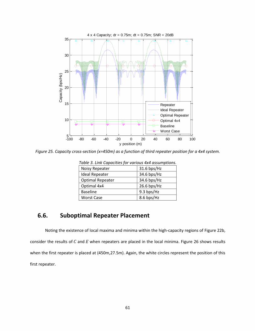
61

Figure 25. Capacity cross-section (x=450m) as a function of third repeater position for a 4x4 system.

Table 3. Link Capacities for various 4x4 assumptions.

Noisy Repeater 31.6 bps/Hz

Ideal Repeater 34.6 bps/Hz

Optimal Repeater 34.6 bps/Hz

Optimal 4x4 26.6 bps/Hz

Baseline 9.3 bps/Hz

Worst Case 8.6 bps/Hz

6.6. Suboptimal Repeater Placement

Noting the existence of local maxima and minima within the high-capacity regions of Figure 22b,

consider the results of and when repeaters are placed in the local minima. Figure 26 shows results

when the first repeater is placed at (450m,27.5m). Again, the white circles represent the position of this

first repeater.

-100 -80 -60 -40 -20 0 20 40 60 80 1005

10

15

20

25

30

35

y position (m)

Capacity (

bps/H

z)


Repeater

Ideal Repeater

Optimal Repeater

Optimal 4x4

Baseline

Worst Case

62

Figure 26. C and E as a function of the second repeater’s position with a suboptimally-placed initial repeater.

Comparing these results with those shown in Figure 23, we note that the available capacity is

still quite high for a second repeater’s placement, but the pattern does change. The optimal placements

are compressed downward since we have moved the repeater farther down the plot. Now consider the

results of and as a function of a third repeater’s position when we place a second repeater at

(450m,-27.5m) as shown in Figure 27.

Figure 27. C and E as a function of the third repeater’s position with two suboptimally-placed initial repeaters.

Comparing these results with Figure 24, note that the suboptimal placement of two repeaters

has reduced the available capacity of the link from a maximum of approximately 34.7bps/Hz to

x position (m)

y p

ositio

n (

m)


0 200 400 600 800 1000

-80

-60

-40

-20

0

20

40

60

80 12

14

16

18

20

22

24

26

x position (m)

y p

ositio

n (

m)


0 200 400 600 800 1000

-80

-60

-40

-20

0

20

40

60

80

0

200

400

600

800

1000

x position (m)

y p

ositio

n (

m)


0 200 400 600 800 1000

-80

-60

-40

-20

0

20

40

60

8020

22

24

26

28

30

32

x position (m)

y p

ositio

n (

m)


0 200 400 600 800 1000

-80

-60

-40

-20

0

20

40

60

80

0

1

2

3

4

5

x 105

63

32.9bps/Hz, a 5% degradation. However, the robustness in available positions for the final repeater are

actually improved by these initial suboptimal placements. For the optimally placed repeaters (Figure 24),

approximately 15.0% of the positions simulated exceed a capacity of 31.2bps/Hz (or 90% of the

34.7bps/Hz maximum). For the suboptimally placed repeaters (Figure 27), 40.7% of the positions exceed

a capacity of 29.6bps/Hz (90% of the 32.9bps/Hz maximum) and 15.5% of the positions exceed a

capacity of 31.2bps/Hz (90% of the 34.7bps/Hz maximum). In terms of percentage of maximum, there is

a significant improvement in repeater position robustness at the expense of a small degradation in

capacity. Relative to an absolute capacity, there is a small improvement in position robustness by

placing initial repeaters in suboptimal locations.

Figure 28 shows the CCDF curves associated with both optimal and suboptimal initial repeater

placements over the entire simulated area. Noting that the shape of the curves will be determined by

the arbitrary cutoff of our range of simulated positions, we are not concerned with the values of the

probabilities, but rather the comparison between them. If the link can be considered successful with

capacities at or below 31bps/Hz, for example, we will likely enjoy better robustness in the placement of

our repeaters using suboptimal placements than we would by using optimal placements. The amount of

robustness obviously depends on the specific implementation, but the example given here illustrates an

interesting possibility in designing higher-order RACE systems for MIMO links.

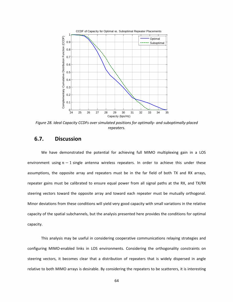
64

Figure 28. Ideal Capacity CCDFs over simulated positions for optimally- and suboptimally-placed

repeaters.

6.7. Discussion

We have demonstrated the potential for achieving full MIMO multiplexing gain in a LOS

environment using single antenna wireless repeaters. In order to achieve this under these

assumptions, the opposite array and repeaters must be in the far field of both TX and RX arrays,

repeater gains must be calibrated to ensure equal power from all signal paths at the RX, and TX/RX

steering vectors toward the opposite array and toward each repeater must be mutually orthogonal.

Minor deviations from these conditions will yield very good capacity with small variations in the relative

capacity of the spatial subchannels, but the analysis presented here provides the conditions for optimal

capacity.

This analysis may be useful in considering cooperative communications relaying strategies and

configuring MIMO-enabled links in LOS environments. Considering the orthogonality constraints on

steering vectors, it becomes clear that a distribution of repeaters that is widely dispersed in angle

relative to both MIMO arrays is desirable. By considering the repeaters to be scatterers, it is interesting

24 25 26 27 28 29 30 31 32 33 34 350

0.1

0.2

0.3

0.4

0.5

0.6

0.7

0.8

0.9

1

Capacity (bps/Hz)

Com

ple

menta

ry C

um

ula

tive D

istr

ibution F

unction (

CC

DF

)

CCDF of Capacity for Optimal vs. Suboptimal Repeater Placements

Optimal

Suboptimal

65

to note the relationship between MIMO array size and the required spread in arrival angle of the

multipath components. When the array size is small, the required spread is quite large, but as the array

size grows, introducing more grating lobes in an equivalent beamforming array, the requirement for

orthogonal steering vectors may be met by a much smaller angular spread of scatterers. This is similar to

the results of certain studies relating angular spread to MIMO capacity in NLOS environments [61-62].

66

Chapter 7: RACE for Point-to-Multipoint LOS MIMO Links

Having investigated the RACE concept for point-to-point links in Chapters 5 and 6, we propose to

extend the analysis in this chapter to a point-to-multipoint link such as might be found in a ground-to-air

sensor network backhaul link or a cellular environment [63]. This requires that we reconsider some of

our system assumptions in order to explore enabling MIMO multiplexing for a large number of

users/nodes simultaneously over a large geographical distribution.

To motivate the ground-to-air sensor network backhaul application, recall from [9-11] that large

antenna spacings can accommodate full multiplexing gain in LOS environments. We therefore note that

an airborne sink with a 2-element MIMO array with spacing of 14.8m (size of Predator wingspan), flying

at 500m (where typical altitudes might range from 2-9km), yields a maximum capacity of 7.8bps/Hz

without repeater assistance. The worst case is 7.65bps/Hz. At typical altitudes, this baseline is closer to

the worst case. The cellular environment has similar limitations with smaller available array sizes at

lower altitudes. The following analysis seeks to improve upon the baseline using RACE.

The system model we propose for this investigation is described in Section 7.1. The analysis in

this paper relies on three different metrics. The first two are the MIMO capacity (21) and determinant

metric (22) and the third is developed in Section 7.3. The channel matrix feeding these metrics is

computed using the channel model described in Section 5.1 (42). Section 7.3 presents simulation results

followed by a discussion in Section 7.4.

7.1. System Model

For this analysis, we will assume the existence of a single RX node at the origin or directly above

the origin somewhere on the positive z-axis. We also assume that the antennas of this node form a

uniform linear array (ULA) with antennas positioned in the +/-y direction so the array normal is in the +/-

x direction. This RX node represents the sensor network sink or fusion center or a cellular base station.

67

For simplicity, we will designate this node the “sink” with the understanding that in the cellular

paradigm, it would be known as the base station. A repeater is positioned to assist the link and the

analysis considers the capacity for a link between the fixed RX node and a TX node at various positions

with various ULA orientations. These TX nodes will be designated as the “sensors,” though they may

represent mobile users for a cellular configuration. Thus, the three components of our system model are

1) the sink (RX), 2) the sensor (TX), and 3) the repeater.

Although multiple repeaters may potentially enable higher-order MIMO links, this analysis is

restricted to or links with a single repeater. Considering the limited form factor of typical

sensor nodes and handheld mobile devices, this seems to be a reasonable constraint. In the cellular

environment, this system configuration represents the uplink portion of the link, but we may easily swap

the TX/RX nodes to represent the downlink. There will be some small variation in capacity when we

swap the link because of noise coloring and amplification introduced by the repeater, but the simulation

results presented here are restricted to the uplink with a brief discussion of the impact of repeater noise

on the downlink results.

The wireless configuration we propose to analyze is shown in Figure 29. In the figure, the

triangles represent TX/RX MIMO antennas, the black squares are the centers of the MIMO arrays, and

the star represents the repeater. The inter-element antenna spacings are given by “ ” and “ ,” the

range by “ ,” and the angle the TX array normal makes with the x-axis is given by .

In order to develop an understanding of the impact of various parameters and to offer a smooth

transition from the results presented in Chapters 5 and 6, initial results in this chapter consider the case

when both the sink and repeater are on the ground and , the inter-element spacing

used in most of the previous analyses. After the initial analysis, the antenna spacing is reduced to more

realistic values for mobile users and sensor nodes and the sink and repeater nodes are made airborne to

explore the capabilities of a RACE system over a ground-to-air channel for multiple ground-based nodes.

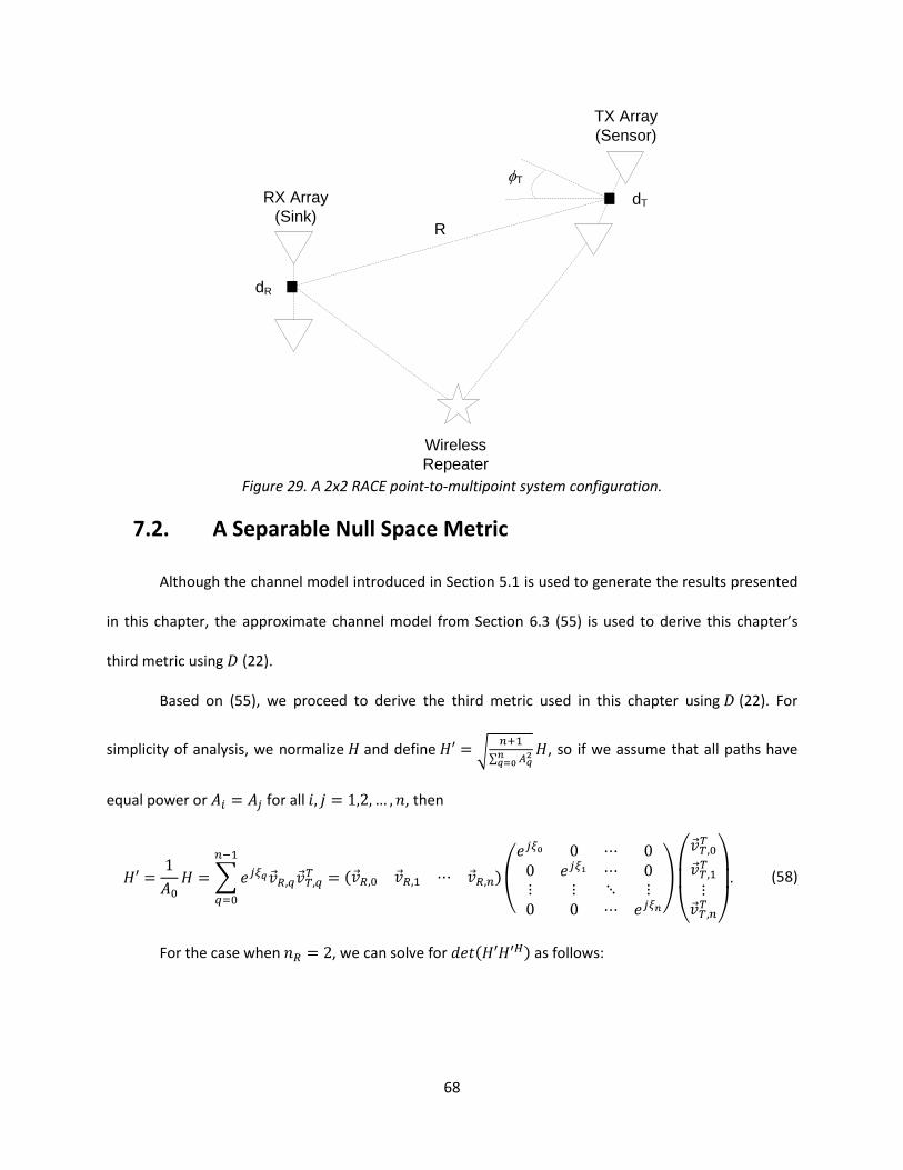
68

T

..RX Array

(Sink)

TX Array

(Sensor)

Wireless

Repeater

dR

dT

R

Figure 29. A 2x2 RACE point-to-multipoint system configuration.

7.2. A Separable Null Space Metric

Although the channel model introduced in Section 5.1 is used to generate the results presented

in this chapter, the approximate channel model from Section 6.3 (55) is used to derive this chapter’s

third metric using (22).

Based on (55), we proceed to derive the third metric used in this chapter using (22). For

simplicity of analysis, we normalize and define , so if we assume that all paths have

equal power or for all , then

(58)

For the case when , we can solve for as follows:

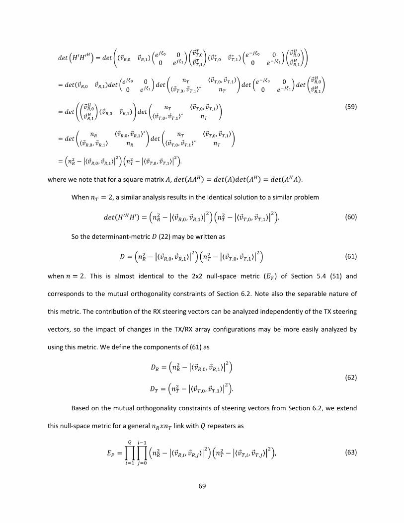
69

(59)

where we note that for a square matrix , .

When , a similar analysis results in the identical solution to a similar problem

(60)

So the determinant-metric (22) may be written as

(61)

when . This is almost identical to the 2x2 null-space metric ( ) of Section 5.4 (51) and

corresponds to the mutual orthogonality constraints of Section 6.2. Note also the separable nature of

this metric. The contribution of the RX steering vectors can be analyzed independently of the TX steering

vectors, so the impact of changes in the TX/RX array configurations may be more easily analyzed by

using this metric. We define the components of (61) as

(62)

Based on the mutual orthogonality constraints of steering vectors from Section 6.2, we extend

this null-space metric for a general link with repeaters as

(63)

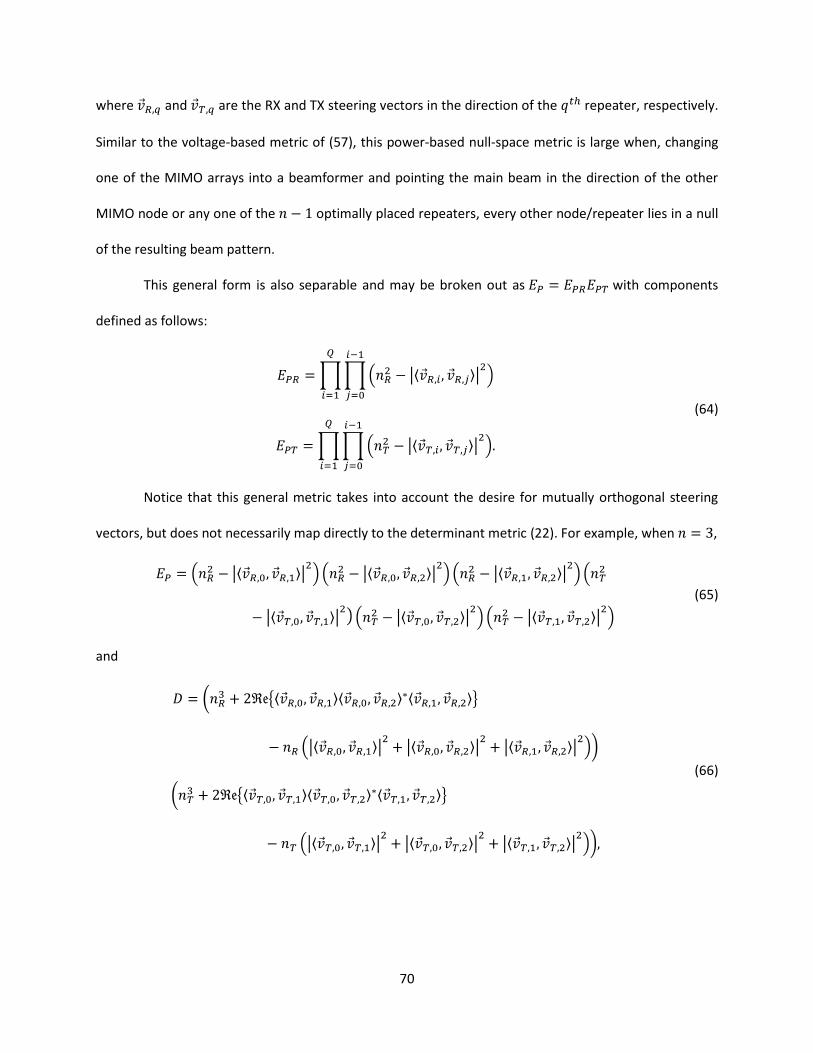
70

where and are the RX and TX steering vectors in the direction of the repeater, respectively.

Similar to the voltage-based metric of (57), this power-based null-space metric is large when, changing

one of the MIMO arrays into a beamformer and pointing the main beam in the direction of the other

MIMO node or any one of the optimally placed repeaters, every other node/repeater lies in a null

of the resulting beam pattern.

This general form is also separable and may be broken out as with components

defined as follows:

(64)

Notice that this general metric takes into account the desire for mutually orthogonal steering

vectors, but does not necessarily map directly to the determinant metric (22). For example, when ,

(65)

and

(66)

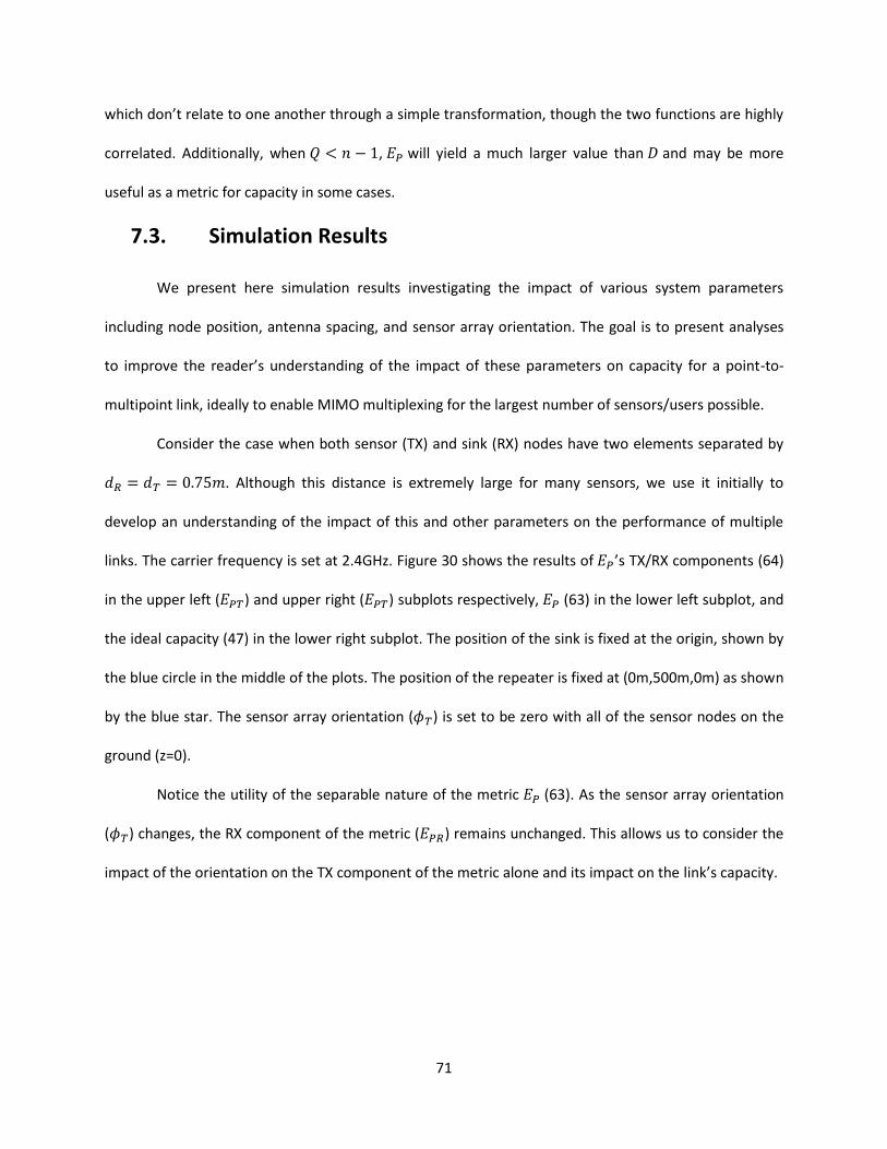
71

which don’t relate to one another through a simple transformation, though the two functions are highly

correlated. Additionally, when , will yield a much larger value than and may be more

useful as a metric for capacity in some cases.


We present here simulation results investigating the impact of various system parameters

including node position, antenna spacing, and sensor array orientation. The goal is to present analyses

to improve the reader’s understanding of the impact of these parameters on capacity for a point-to-

multipoint link, ideally to enable MIMO multiplexing for the largest number of sensors/users possible.

Consider the case when both sensor (TX) and sink (RX) nodes have two elements separated by

. Although this distance is extremely large for many sensors, we use it initially to

develop an understanding of the impact of this and other parameters on the performance of multiple

links. The carrier frequency is set at 2.4GHz. Figure 30 shows the results of ’s TX/RX components (64)

in the upper left ( ) and upper right ( ) subplots respectively, (63) in the lower left subplot, and

the ideal capacity (47) in the lower right subplot. The position of the sink is fixed at the origin, shown by

the blue circle in the middle of the plots. The position of the repeater is fixed at (0m,500m,0m) as shown

by the blue star. The sensor array orientation ( ) is set to be zero with all of the sensor nodes on the

ground (z=0).

Notice the utility of the separable nature of the metric (63). As the sensor array orientation

( ) changes, the RX component of the metric ( ) remains unchanged. This allows us to consider the

impact of the orientation on the TX component of the metric alone and its impact on the link’s capacity.

72

Figure 30. EP, EPR, EPT, and C results for dR=dT=0.75m; φT=0; circle=sink position; star=repeater position.

For the upper two subplots, notice the existence of 24 “rays” emanating from the sink node.

This is of interest because the inter-element antenna spacing used to generate these results ( ) is

equal to 6 . In , these rays wrap around and terminate at the repeater, but in , they extend to

infinity. Observe that close to the sink, both components are nearly identical, indicating that a repeater

placed very far from the service area may make for a more predictable pattern of MIMO-enabled area.

As an example, zooming in around the origin by a factor of 10 results in nearly identical patterns in the

first two subplots of Figure 30.

For the same scenario, Figure 31 shows the required repeater gain for various sensor

positions (upper left) as well as the baseline capacity ( , the capacity of the link without repeater

assistance) in the upper right, and the colored capacity and ideal capacity in the lower left and right

subplots respectively.

x axis (m)

y a

xis

(m

)

ET (TX Null Space Metric)

-1000 0 1000

-1000

-500

0

500

1000

x axis (m)

y a

xis

(m

)

ER (RX Null Space Metric)

-1000 0 1000

-1000

-500

0

500

1000

x axis (m)

y a

xis

(m

)

E=ETE

R (Null Space Metric);

-1000 0 1000

-1000

-500

0

500

1000

x axis (m)

y a

xis

(m

)

Ideal Capacity

-1000 0 1000

-1000

-500

0

500

1000

0

1

2

3

4

0

1

2

3

5

10

15

0

5

10

15

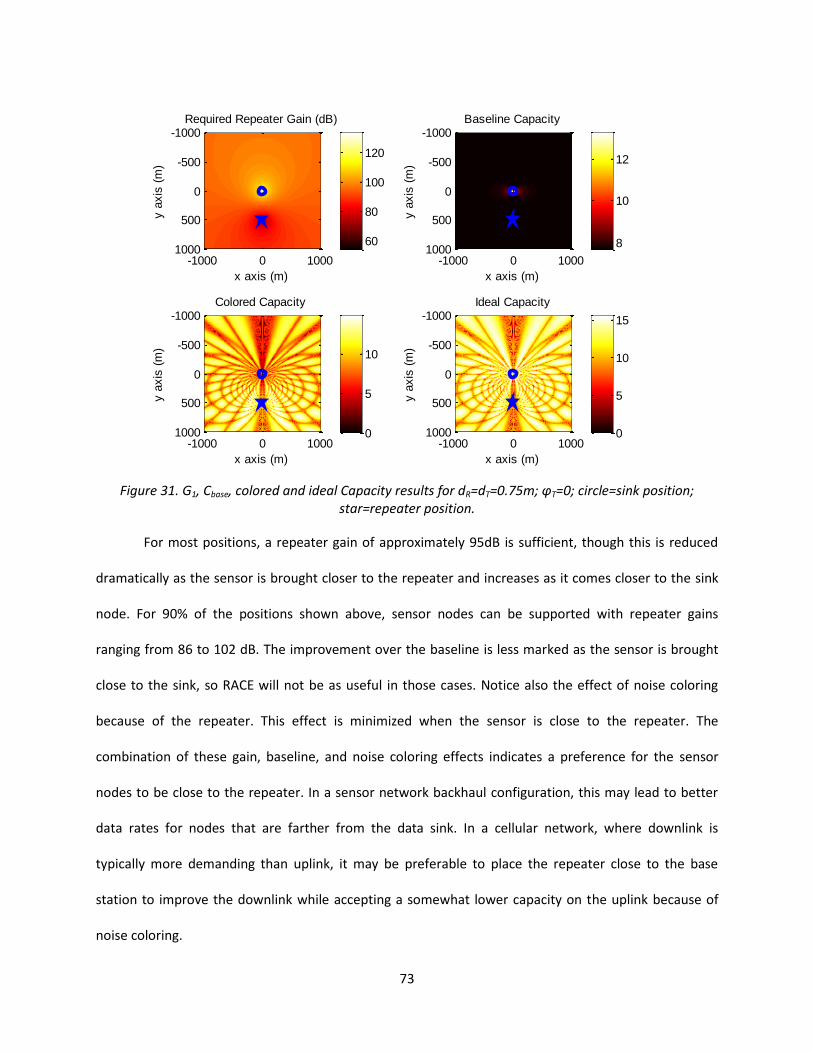
73

Figure 31. G1, Cbase, colored and ideal Capacity results for dR=dT=0.75m; φT=0; circle=sink position;

star=repeater position.

For most positions, a repeater gain of approximately 95dB is sufficient, though this is reduced

dramatically as the sensor is brought closer to the repeater and increases as it comes closer to the sink

node. For 90% of the positions shown above, sensor nodes can be supported with repeater gains

ranging from 86 to 102 dB. The improvement over the baseline is less marked as the sensor is brought

close to the sink, so RACE will not be as useful in those cases. Notice also the effect of noise coloring

because of the repeater. This effect is minimized when the sensor is close to the repeater. The

combination of these gain, baseline, and noise coloring effects indicates a preference for the sensor

nodes to be close to the repeater. In a sensor network backhaul configuration, this may lead to better

data rates for nodes that are farther from the data sink. In a cellular network, where downlink is

typically more demanding than uplink, it may be preferable to place the repeater close to the base

station to improve the downlink while accepting a somewhat lower capacity on the uplink because of

noise coloring.

x axis (m)

y a

xis

(m

)

Required Repeater Gain (dB)

-1000 0 1000

-1000

-500

0

500

1000

x axis (m)

y a

xis

(m

)

Baseline Capacity

-1000 0 1000

-1000

-500

0

500

1000

x axis (m)

y a

xis

(m

)

Colored Capacity

-1000 0 1000

-1000

-500

0

500

1000

x axis (m)

y a

xis

(m

)

Ideal Capacity

-1000 0 1000

-1000

-500

0

500

1000

60

80

100

120

8

10

12

0

5

10

0

5

10

15

74

7.3.1. Sensor Array Orientation

Note that these and most of the subsequent figures present results where is assumed to be

zero. We briefly explore the impact of this parameter and discuss methods for dealing with unfavorable

orientations. Figure 32 shows results similar to those shown in Figure 30 with the same parameters

except that .



Notice the reduced capacity in the direction indicated by the dashed line at an angle of 60o. For

this figure and the next, we have expanded the range of simulated positions by a factor of two in both

dimensions to illustrate this reduced capacity more clearly. This low capacity along that line implies poor

performance for arrays whose normals are perpendicular to the vector connecting the sensor and sink

array centers. Figure 33 corroborates this perpendicular assumption by showing the results where we

set where low capacity is observed along the line indicated by the dashed line at an

x axis (m)

y a

xis

(m

)


-2000 0 2000

-2000

0

2000

1

2

3

x axis (m)

y a

xis

(m

)


-2000 0 2000

-2000

0

2000 0

1

2

3

x axis (m)

y a

xis

(m

)

E=ETE

R (Null Space Metric)

-2000 0 2000

-2000

0

2000 0

5

10

15

x axis (m)

y a

xis

(m

)

Ideal Capacity

-2000 0 2000

-2000

0

2000

5

10

15

75

angle of 45o. This turns out to be the case when the sensor is far away from the sink, with less clarity as

that distances diminishes.



By considering various non-zero values of in simulation like the two results shown above, the

author has determined that orientations where the sensor array normal is orthogonal to the line

connecting the two MIMO arrays typically experience significantly degraded capacities. This orthogonal

state is illustrated in Figure 34.

x axis (m)

y a

xis

(m

)


-2000 0 2000

-2000

0

2000

x axis (m)

y a

xis

(m

)


-2000 0 2000

-2000

0

2000

x axis (m)

y a

xis

(m

)

E=ETE

R (Null Space Metric)

-2000 0 2000

-2000

0

2000

x axis (m)

y a

xis

(m

)Ideal Capacity

-2000 0 2000

-2000

0

2000

1

2

3

0

1

2

3

0

5

10

15

5

10

15

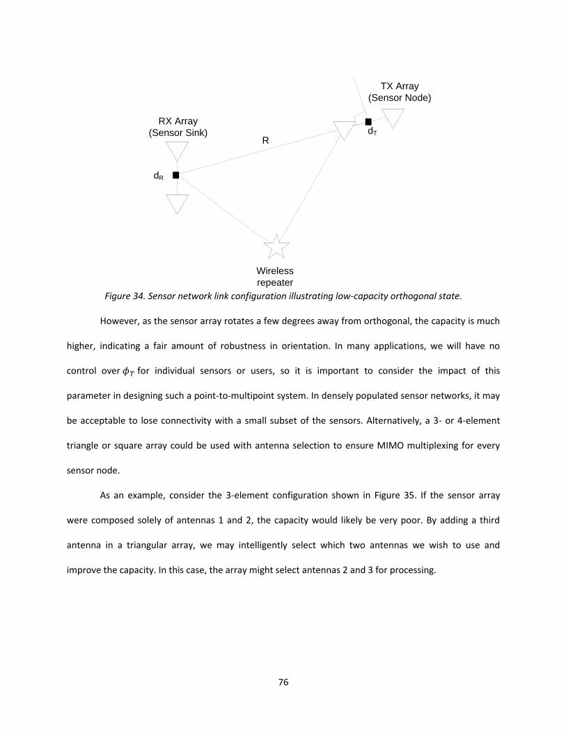
76

..RX Array

(Sensor Sink)

TX Array

(Sensor Node)

Wireless

repeater

dR

dT

R

Figure 34. Sensor network link configuration illustrating low-capacity orthogonal state.

However, as the sensor array rotates a few degrees away from orthogonal, the capacity is much

higher, indicating a fair amount of robustness in orientation. In many applications, we will have no

control over for individual sensors or users, so it is important to consider the impact of this

parameter in designing such a point-to-multipoint system. In densely populated sensor networks, it may

be acceptable to lose connectivity with a small subset of the sensors. Alternatively, a 3- or 4-element

triangle or square array could be used with antenna selection to ensure MIMO multiplexing for every

sensor node.

As an example, consider the 3-element configuration shown in Figure 35. If the sensor array

were composed solely of antennas 1 and 2, the capacity would likely be very poor. By adding a third

antenna in a triangular array, we may intelligently select which two antennas we wish to use and

improve the capacity. In this case, the array might select antennas 2 and 3 for processing.

77

.1

2RX Array

(Sensor Sink)

TX Array

(Sensor Node)

Wireless

repeater

3

Figure 35. Sensor network link configuration illustrating a possible 3-element TX array.

7.3.2. Sensor/Sink Antenna Spacing

Consider now the parameters dictating antenna spacing ( and ). In a sensor network

backhaul configuration, it may be possible for large antenna spacing on the sink, but most likely not for

the ground-based sensor nodes. With this in mind, Figure 36 shows results when and

to accommodate limited space on the sensor platforms.

Notice the change in . Instead of 24 high-value rays connecting sink and repeater, with

spacing, there are only two. This should lead to more continuity in the space of MIMO-enabled nodes

leading to more robust coverage. Considering this relationship between antenna spacing and position

robustness, consider the case when shown in Figure 37.

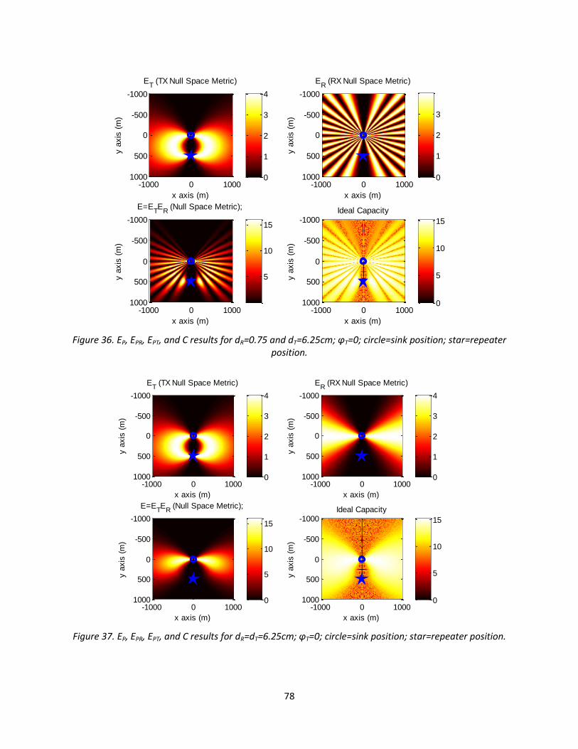
78

Figure 36. EP, EPR, EPT, and C results for dR=0.75 and dT=6.25cm; φT=0; circle=sink position; star=repeater

position.

Figure 37. EP, EPR, EPT, and C results for dR=dT=6.25cm; φT=0; circle=sink position; star=repeater position.

x axis (m)

y a

xis

(m

)


-1000 0 1000

-1000

-500

0

500

1000 0

1

2

3

4

x axis (m)

y a

xis

(m

)


-1000 0 1000

-1000

-500

0

500

1000 0

1

2

3

x axis (m)

y a

xis

(m

)

E=ETE


-1000 0 1000

-1000

-500

0

500

1000

5

10

15

x axis (m)

y a

xis

(m

)

Ideal Capacity

-1000 0 1000

-1000

-500

0

500

1000 0

5

10

15

x axis (m)

y a

xis

(m

)


-1000 0 1000

-1000

-500

0

500

1000 0

1

2

3

4

x axis (m)

y a

xis

(m

)


-1000 0 1000

-1000

-500

0

500

1000 0

1

2

3

4

x axis (m)

y a

xis

(m

)

E=ETE


-1000 0 1000

-1000

-500

0

500

1000 0

5

10

15

x axis (m)

y a

xis

(m

)

Ideal Capacity

-1000 0 1000

-1000

-500

0

500

1000 0

5

10

15

79

Notice the improved robustness of sensor position using smaller array sizes at both ends of the

link. Given the continuity of MIMO-enabled area observed here, it may be desirable for the sink node to

have small spacing for robustness while the sensor may likely have small spacing because of form factor

constraints. It may also be possible to enable MIMO for the parts of the space not served by the first

repeater by employing a second repeater with a beam focused on those low capacity areas. This may

enable the system to provide coverage for the entire immediate area surrounding the sink node from

low altitudes.

7.3.3. Sink/Repeater Altitude

So far, all of the results presented have assumed ground-based sink, sensor, and repeater. This

has allowed us to examine certain behaviors of the link and discuss the impact of various parameters to

some extent. However, the target applications of ground-to-air sensor network backhaul and cellular

systems require the sink and possibly the repeater to be elevated. Figure 39 shows results for the case

when the sink and repeater platforms are raised to an altitude of 500m. This airborne scenario is

represented in Figure 38 showing UAV platforms carrying the sink and repeater nodes collecting

information from ground-based sensor nodes.

This altitude is fairly low for a UAV employed in collecting ground-based sensor data, but quite

high for a tower-based cellular base station. However, by forcing the altitude to be equal to the RX-to-

repeater spacing, we find significant robustness in TX positioning and note that most of the results scale

well by keeping these distances equal.

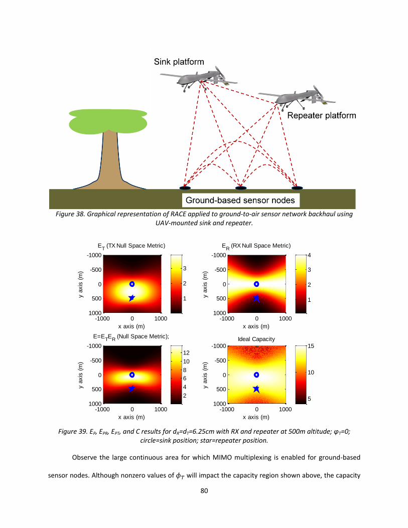
80

Figure 38. Graphical representation of RACE applied to ground-to-air sensor network backhaul using

UAV-mounted sink and repeater.

Figure 39. EP, EPR, EPT, and C results for dR=dT=6.25cm with RX and repeater at 500m altitude; φT=0;

circle=sink position; star=repeater position.

Observe the large continuous area for which MIMO multiplexing is enabled for ground-based

sensor nodes. Although nonzero values of will impact the capacity region shown above, the capacity

x axis (m)

y a

xis

(m

)


-1000 0 1000

-1000

-500

0

500

1000

x axis (m)

y a

xis

(m

)


-1000 0 1000

-1000

-500

0

500

1000

x axis (m)

y a

xis

(m

)

E=ETE


-1000 0 1000

-1000

-500

0

500

1000

x axis (m)

y a

xis

(m

)

Ideal Capacity

-1000 0 1000

-1000

-500

0

500

1000

1

2

3

1

2

3

4

2

4

6

8

10

12

5

10

15

81

is fairly robust to changes in sensor array orientation that are not too close to the orthogonal constraint

described previously. Averaged over all values of , the high-capacity region is fairly close to that

depicted above.

Though not pictured here, the required repeater gain ranges from about 90 to 98dB and the

baseline capacity is approximately 7.65bps/Hz for every ground-based sensor position. If the sink-to-

repeater distance and sink/repeater altitudes are set to 5000m, the graphs look nearly identical to those

shown in Figure 39, the only notable difference being that the required repeater gain ranges from 110 to

118dB, an increase of 20dB for a factor of 10 increase in the distances.

7.4. Discussion

The use of the RACE concept has been investigated for enabling MIMO multiplexing in a LOS

point-to-multipoint link such as a ground-to-air sensor network backhaul or cellular configuration. Using

a single repeater, such a system can enable multiplexing for a large number of users offering nearly

twice the capacity of the system without repeater assistance. Several system parameters were

investigated in simulation to determine their impact on the multiple links with a view toward improving

capacity for the maximum number of sensors or users. Robustness in position/orientation of these

nodes is therefore desirable.

Some of the parameters investigated include inter-element antenna spacing, TX orientation, and

RX/repeater positioning in 3-D. With the RX representing a data sink or fusion center for sensor

backhaul applications or a base station for cellular configurations, we assume that large arrays may be

accommodated by the sink, but not necessarily by the sensor platform. Large arrays tend to improve

capacity at longer ranges, but with less robustness or continuity in sensor node positioning. Smaller

arrays offer continuity and robustness at the expense of range.

Raising the sink and repeater nodes in altitude can also improve sensor position robustness and

compress the range of repeater gains required to enable full multiplexing for a large area. The effects of

82

noise coloring and amplification because of the presence of the repeater tend to favor links where the

sensor is closer to the repeater than to the sink. In sensor backhaul, this leads to better connectivity to

nodes farther from the data sink. In cellular, where downlink may require higher data rates than uplink,

it may be desirable to place the repeater fairly close to the base station.

The orientation of the sensor nodes, while presumably uncontrollable, degrades capacity when

the sensor array normal is orthogonal to the line connecting the sensor and sink arrays (see Figure 34).

This degradation is restricted to a small range of angles close to the orthogonal constraint and may be

mitigated by a triangle or square array and selecting the two most favorable antennas in the array for

communication.

Although the results presented here are restricted to the single repeater case, multiple

repeaters may be employed to expand the area of MIMO-enabled coverage or further enhance

multiplexing. Theoretically, it is possible to yield capacity improvements of a factor of using

repeaters.

83

Chapter 8: Conclusions

We conclude the investigation of LOS MIMO capacity limitations and enhancements by

reviewing the novel contributions presented in this dissertation and discussing possible future avenues

for further investigation.

8.1. Contributions

In this dissertation, we have considered the limitations on MIMO capacity in a LOS environment.

In doing so, we have made the following novel contributions:

1) a novel development of the optimal form of a MIMO channel matrix in Section 3.2;

2) the development of a determinant-based metric ( ) for analyzing MIMO capacity in Sections 3.1

and 4.1;

3) a theoretic analysis of upper and lower capacity bounds as a function of in Section 4.2;

4) an introduction of a repeater-assisted capacity enhancement (RACE) method for enhancing LOS

MIMO capacity in Chapter 5;

5) a detailed simulation-based analysis of repeater position using RACE for a given point-to-point

link configuration in Section 5.3;

6) an introduction of a position-based metric and method of repeater placement in Sections 5.4

and 7.3;

7) a theoretical analysis of repeater position for a general MIMO link in Chapter 6; and

8) an investigation of RACE for point-to-multipoint links with a discussion of the impact of system

parameters on coverage size and robustness in Chapter 7.

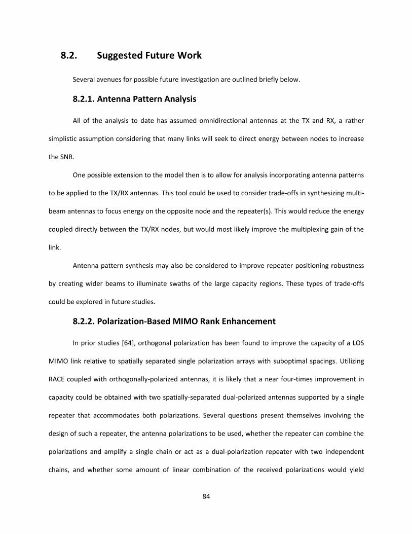
84

8.2. Suggested Future Work

Several avenues for possible future investigation are outlined briefly below.

8.2.1. Antenna Pattern Analysis

All of the analysis to date has assumed omnidirectional antennas at the TX and RX, a rather

simplistic assumption considering that many links will seek to direct energy between nodes to increase

the SNR.

One possible extension to the model then is to allow for analysis incorporating antenna patterns

to be applied to the TX/RX antennas. This tool could be used to consider trade-offs in synthesizing multi-

beam antennas to focus energy on the opposite node and the repeater(s). This would reduce the energy

coupled directly between the TX/RX nodes, but would most likely improve the multiplexing gain of the

link.

Antenna pattern synthesis may also be considered to improve repeater positioning robustness

by creating wider beams to illuminate swaths of the large capacity regions. These types of trade-offs

could be explored in future studies.

8.2.2. Polarization-Based MIMO Rank Enhancement

In prior studies [64], orthogonal polarization has been found to improve the capacity of a LOS

MIMO link relative to spatially separated single polarization arrays with suboptimal spacings. Utilizing

RACE coupled with orthogonally-polarized antennas, it is likely that a near four-times improvement in

capacity could be obtained with two spatially-separated dual-polarized antennas supported by a single

repeater that accommodates both polarizations. Several questions present themselves involving the

design of such a repeater, the antenna polarizations to be used, whether the repeater can combine the

polarizations and amplify a single chain or act as a dual-polarization repeater with two independent

chains, and whether some amount of linear combination of the received polarizations would yield

85

improved performance over simply amplifying and relaying both modes. An investigation into the

impact of such an extension would be interesting, if only to validate the claim that a near four-times

capacity improvement may be obtained with a single repeater.

8.2.3. Rigorous Repeater Model

The repeater model currently incorporates the effect of colored noise and noise amplification,

but does not allow for feedback or cross-talk between multiple repeaters. The modeling of feedback and

cross-talk would be a useful extension of the current model and could be accomplished using the

Wittneben-based colored noise / noise amplification model [33] described in Section 5.2. The dual-

repeater model could be represented by Figure 40. The -repeater model is a simple extension of this,

but is difficult to represent clearly in a figure.

The T-parameters form a 2x2 (or in general, a ) feedback matrix where the diagonal

elements represent self-feedback based on repeater isolation and the off-diagonal elements represent

cross-talk. These values would depend on antenna patterns, which would have to be added to the

model as described in Section 8.2.1. These T-parameters could be modeled and the feedback added to

the simulation tool to explore stability issues.

Figure 40. System model for incorporating repeater feedback and cross-talk.

H0

H11

H21

x

+

+

nr1

nr2

G1

G2

H12

H22

+ y

n

y0

y1

y2

T11

T22

T12

T21

r1

r2

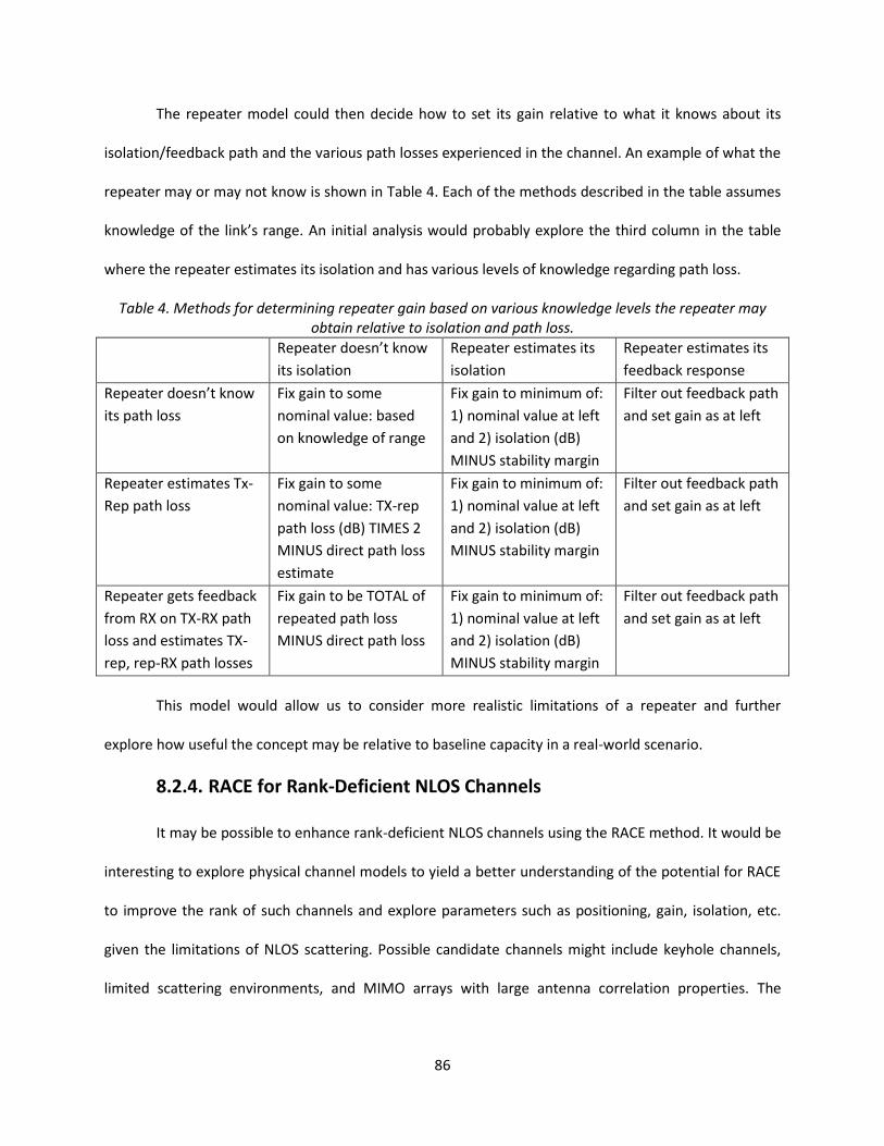
86

The repeater model could then decide how to set its gain relative to what it knows about its

isolation/feedback path and the various path losses experienced in the channel. An example of what the

repeater may or may not know is shown in Table 4. Each of the methods described in the table assumes

knowledge of the link’s range. An initial analysis would probably explore the third column in the table

where the repeater estimates its isolation and has various levels of knowledge regarding path loss.

Table 4. Methods for determining repeater gain based on various knowledge levels the repeater may obtain relative to isolation and path loss.

Repeater doesn’t know

its isolation

Repeater estimates its

isolation

Repeater estimates its

feedback response

Repeater doesn’t know

its path loss

Fix gain to some

nominal value: based

on knowledge of range

Fix gain to minimum of:

1) nominal value at left

and 2) isolation (dB)

MINUS stability margin

Filter out feedback path

and set gain as at left

Repeater estimates Tx-

Rep path loss

Fix gain to some

nominal value: TX-rep

path loss (dB) TIMES 2

MINUS direct path loss

estimate







Repeater gets feedback

from RX on TX-RX path

loss and estimates TX-

rep, rep-RX path losses

Fix gain to be TOTAL of

repeated path loss

MINUS direct path loss







This model would allow us to consider more realistic limitations of a repeater and further

explore how useful the concept may be relative to baseline capacity in a real-world scenario.

8.2.4. RACE for Rank-Deficient NLOS Channels

It may be possible to enhance rank-deficient NLOS channels using the RACE method. It would be

interesting to explore physical channel models to yield a better understanding of the potential for RACE

to improve the rank of such channels and explore parameters such as positioning, gain, isolation, etc.

given the limitations of NLOS scattering. Possible candidate channels might include keyhole channels,

limited scattering environments, and MIMO arrays with large antenna correlation properties. The

87

extension to NLOS channel models could present very difficult challenges in correlating with physical

environments to develop an understanding for optimal repeater placement.

8.2.5. RACE for Passive Sensor Backhaul

Extending the analysis in Chapter 7, it would be interesting to explore the feasibility of sensor

network backhaul using passive sensor nodes. This configuration assumes the absence of a power

amplifier in the sensor node and requires additional power and/or receiver sensitivity in the airborne

interrogator. This may also have applicability to high-capacity RFID systems in LOS environments. The

channel model would need to be extended to incorporate double-bounce propagation. The channel is

likely best modeled as a product Rician fading channel [65] and certainly behaves differently than the

single fading channel. Such an analysis could build off the simulation framework described in this

dissertation, but will require some channel analysis in the context of radar signal processing. The sensor

node in this case may encode its data by modifying the impedance seen at the antenna in order to

create a “modulated backscatter” signal as seen at the interrogator *66]. This signal would have to be

detected in the presence of ground clutter, much as a radar signal of interest would be processed. Initial

work could include efforts to better understand the bounds of the problem including limitations on

range, and trade-offs between modulation scheme, data rate, Doppler spectrum offset, and SNR

requirements. With a clear understanding of these limitations and a suitable channel model, the RACE

concept could be applied in the context of the realistic scenarios identified by the initial investigation.

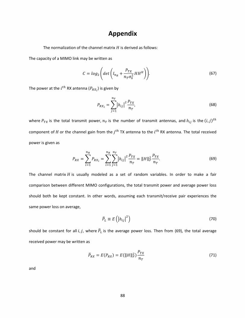
88

Appendix

The normalization of the channel matrix is derived as follows:

The capacity of a MIMO link may be written as

(67)

The power at the RX antenna ( ) is given by

(68)

where is the total transmit power, is the number of transmit antennas, and is the

component of or the channel gain from the TX antenna to the RX antenna. The total received

power is given as

(69)

The channel matrix is usually modeled as a set of random variables. In order to make a fair

comparison between different MIMO configurations, the total transmit power and average power loss

should both be kept constant. In other words, assuming each transmit/receive pair experiences the

same power loss on average,

(70)

should be constant for all , where is the average power loss. Then from (69), the total average

received power may be written as

(71)

and

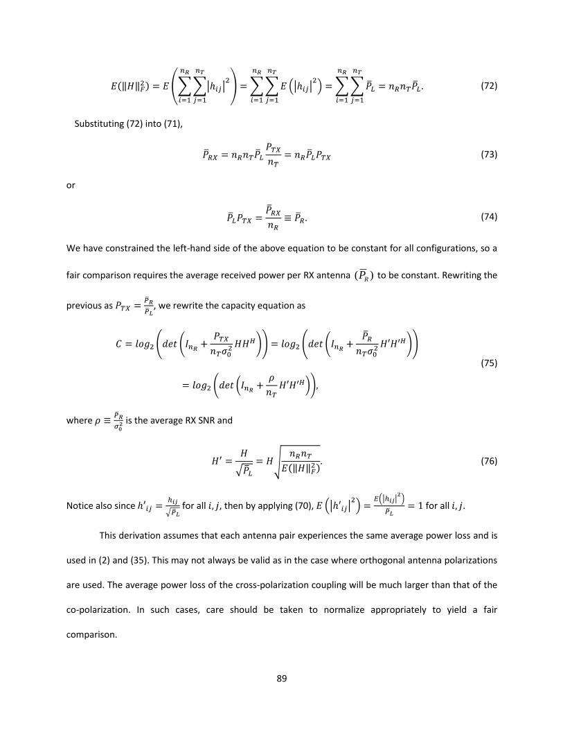
89

(72)

Substituting (72) into (71),

(73)

or

(74)

We have constrained the left-hand side of the above equation to be constant for all configurations, so a

fair comparison requires the average received power per RX antenna )( RP to be constant. Rewriting the

previous as , we rewrite the capacity equation as

(75)

where is the average RX SNR and

(76)

Notice also since for all , then by applying (70), for all .

This derivation assumes that each antenna pair experiences the same average power loss and is

used in (2) and (35). This may not always be valid as in the case where orthogonal antenna polarizations

are used. The average power loss of the cross-polarization coupling will be much larger than that of the

co-polarization. In such cases, care should be taken to normalize appropriately to yield a fair

comparison.

90

Specifically, would be dictated by the power loss of an antenna pair common to both

configurations (i.e. vertical to vertical polarization). would then be equal to 1 only for those

antenna pairs. In this case, can no longer be properly defined as the average received power per

antenna, but should nevertheless be kept constant to make a fair comparison.

91

References

1. C.E. Shannon, “A mathematical theory of communication,” The Bell System Technical Journal, Vol. 27,

pp. 379-423, July 1948.

2. G.J. Foschini and M.J. Gans, “On limits of wireless Communications in fading environment when

using multiple antennas,” Wireless Pers. Commun. Vol 6, pp. 331-335, Mar 1998.

3. E. Biglieri, R. Calderbank, A. Constantinides, A. Goldsmith, A. Paulraj, and H.V. Poor, MIMO Wireless

Communications, Cambridge University Press, 2007.

4. M.N. Patwary, P.B. Rapajic, J. Choi, “Decision feedback MLSE for spatially multiplexed MIMO

frequency selecting fading channel,” IEE Proceedings Communications, vol. 153, no. 1, pp. 39-48, Feb

2006.

5. T. Taniguchi, N.B. Ramli, Y. Karasawa, “Spatio-temporal MIMO systems for multiuser

communications under frequency selective fading,” International Conference on Digital

Telecommunications, pp. 8-13, Aug 2006.

6. K.K. Wong, R.D. Murch, K.B. Letaief, “MIMO antenna system for frequency selective fading channels,”

IEEE PIMRC, vol. 2, pp. 1500-1504, Sep 2000.

7. Eugene, C.H.Y. Sakaguchi, K. Araki, K., “Experimental and analytical investigation of MIMO channel

capacity in an indoor line-of-sight (LOS) environment,” Proc. IEEE PIMRC, Sept 2004.

8. Zhongwei Tang, Mohan, A.S., “Experimental investigation of indoor MIMO ricean channel capacity,”

Antennas and Wireless Propagation Letters, vol. 4, pp 55-58, 2005.

9. J.S. Jiang and M.A. Ingram, “Spherical-wave model for short-range MIMO,” IEEE Trans. Comm., Vol.

53, pp. 1534-1541, Sep 2005.

10. F. Bøhagen, P. Orten, and G.E. Øien, “Design of optimal high-rank line-of-sight MIMO channels,” IEEE

Trans. on Wireless Communications, pp 1420-1425, Apr 2007.

11. I. Sarris, A.R. Nix, “Capacity evaluation of los-optimised and standard MIMO antenna arrays at 5.2

GHz,” IEEE VTC, Apr 2007.

12. I. Sarris, A.R. Nix, “Maximum MIMO capacity in line-of-sight,” 5th International Conference on

Information, Communications and Signal Processing, pp. 1236-1240, Dec 2005.

13. J. Jiang and M.A. Ingram, “Distributed source model for short-range MIMO,” Vehicular Technology

Conference, vol. 1, pp. 357-362, Oct 2003.

14. A. Knopp, C.A. Hofmann, M. Chouayakh, B. Lankl, “Exploiting single SISO impulse responses to

predict the capacity of correlated MIMO channels,” Globecom, pp. 3184-3189, Nov 2007.

15. A. Knopp, R.T. Schwarz, C.A. Hofmann, M. Chouayakh, B. Lankl, “Measurements on the impact of

sparse multipath components on the LOS MIMO channel capacity,” 4th ISWCS, pp. 55-60, Oct 2007.

16. T. Haustein and U. Krüger, “Smart geometrical antenna design exploiting the LOS component to

enhance a MIMO system based on rayleigh-fading in indoor scenarios,” in Proc. IEEE PIMRC, Beijing,

China, pp. 1144-1148, Sep 2003.

17. A.A. Hutter, F. Platbrood, and J. Ayadi, “Analysis of MIMO capacity gains for indoor propagation

92

channels with LOS component,” in Proc. IEEE PIMRC, Lisbon, Portugal, pp. 1337-1347, Sept 2002.

18. B.T. Walkenhorst, T.G. Pratt, M.A. Ingram, “Improving MIMO capacity in a line-of-sight environment,”

IEEE Globecom, pp. 3623-3628, Nov 2007.

19. B.T. Walkenhorst, M.A. Ingram, “Repeater-assisted capacity enhancement (RACE) for MIMO links in

a line-of-sight environment,” IEEE International Conference on Communications, Jun 2009.

20. C.R. Anderson, et al, “Antenna isolation, wideband multipath propagation measurements, and

interference mitigation for on-frequency repeaters,” IEEE Proceedings of SoutheastCon, pp 110-114,

Mar 2004.

21. A.S.M. Marzuki, et al, “Antenna isolation considerations in WCDMA repeater deployment,”

International RF and Microwave Conference, pp. 347-350, Sep 2006.

22. W.T. Slingsby and J.P. McGeehan, “Antenna isolation measurements for on-frequency radio

repeaters,” 9th International Conference on Antennas and Propagation, pp 239-243, Apr 1995.

23. P.M. Slobodzian, “Estimation of the repeater gain for a wireless link,” 15th International Conference

on Microwaves, Radar and Wireless Communications, pp. 656-659, May 2004.

24. K.M. Nasr, et al, “Performance of an echo-canceller and channel estimator for on-channel repeaters

in DVB-T/H networks,” IEEE Trans. on Broadcasting, vol. 53, pp. 609-618, 2007.

25. S. Zhao, et al, “A unit with functions of spectrum monitoring, self-excitation detection and isolation

degree test for wireless relay station,” IEEE VTC, vol. 3, pp 1554-1557, Apr 2003.

26. R.N. Braithwaite, “Estimation and compensation of radiated feedback coupling in a high gain

repeater using gain dithering,” European Conference on Wireless Technologies, pp. 197-200, Oct

2007.

27. A. Grau, et al, “Back-to-back high-isolation iso-frequency repeater antenna using MEMS-

reconfigurable-parasitics,” IEEE Antennas and Propagation International Symposium, pp. 497-500,

Jun 2007.

28. E. C. van der Meulen, Transmission of information in a T-terminal discrete memoryless channel, PhD thesis, Dept. of Statistics, University of California, Berkeley, 1968.

29. T.M. Cover and A. A. El Gamal, "Capacity theorems for the relay channel," IEEE Trans. Inform. Theory, Vol. 25, pp. 572-584, 1979.

30. M.A. Khojastepour, Distributed Cooperative Communications in Wireless Networks, PhD Thesis, Department of Electrical and Computer Engineering, Rice University, 2004.

31. J. N. Laneman, D. N. C. Tse, and G. W. Wornell, "Cooperative diversity in wireless networks: efficient protocols and outage behavior," IEEE Trans. Information Theory, Vol. 50, pp. 3062-3080, 2004.

32. A.Chakrabarti, A. Sabharwal, B. Aazhang, "Cooperative communications- fundamental limits and practical implementation," Cooperation in Wireless Networks: Principles and Applications, F. P. Fitzek and M. D. Katz, eds. Springer, pp. 29-68, 2006.

33. A. Wittneben, B. Rankov, "Impact of cooperative relays on the capacity of rank-deficient MIMO channels," Proceedings of the 12th IST Summit on Mobile and Wireless Communications, Aveiro, Portugal, pp. 421-425, June 2003.

93

34. L Tsai, D. Shiu, “Channel modeling and capacity evaluation for relay-aided MIMO systems in LOS environments,” International Symposium on Communications and Information Technologies, pp. 796-801, Oct 2007.

35. B. Wang, Z. Han; K.J.R. Liu, “Stackelberg game for distributed resource allocation over multiuser cooperative communication networks,” IEEE Global Telecommunications Conference, pp. 1-5, Nov 2006.

36. I. Ahmed, M. Peng, W. Wang, “Energy efficient cooperative nodes selection in wireless sensor networks,” International Conference on Parallel Processing Workshops, pp. 50-54, Sep 2007.

37. L. Fei; L. Qinghua; L. Tao; Y. Guangxin, “Impact of relay location according to SER for amplify-and-forward cooperative communications,” IEEE International Workshop on Anti-counterfeiting, Security, Identification, pp. 324-327, Apr 2007.

38. A.Chakrabarti, A. Sabharwal, B. Aazhang, "Cooperative communications- fundamental limits and practical implementation," Cooperation in Wireless Networks: Principles and Applications, F. P. Fitzek and M. D. Katz, eds. Springer, pp. 29-68, 2006.

39. Y. Fan and J. Thompson, “MIMO configurations for relay channels: theory and practice,” IEEE Trans

Wireless Comm, vol 6, no 5, pp. 1774-1786, May 2007.

40. Y. Fan, H.V. Poor, J.S. Thompson, “Cooperative multiplexing in a half duplex relay network:

performance and constraints,” submitted to IEEE Transactions on Communications, June 2007.

41. M. Yuksel and E. Erkip, “Diversity-multiplexing tradeoff in half-duplex relay systems,” Proceedings of

IEEE International Conference on Communications, pp 689-694, Jun 2007.

42. R.U. Nabar, H. Bolcskei, F.W. Kneubuhler, “Fading relay channels: performance limits and space-time

signal design,” IEEE Journal on Selected Areas of Communications, vol 22, pp. 1099-1109, Aug 2004.

43. O. Fernandez, M. Domingo, R.P. Torres, “Simple adaptive system to improve MIMO channel

capacity,” published by the 29th URSI General Assembly, Oct 2005.

44. F. Jingxing, Y. Dacheng, M. Min, “A novel V-BLAST detection algorithm,” ICCT, vol 2, pp. 1202-1205,

2003.

45. V. Erceg, P. Soma, D.S. Baum, A.J. Paulraj, “Capacity obtained from multiple-input multiple-output

channel measurements in fixed wireless environments at 2.5 GHz,” ICC, vol 1, pp. 396-400, 2002.

46. J. Brenner and L. Cummings, “The Hadamard maximum determinant problem,” American

Mathematical Monthly 79, pp 626-630, 1972.

47. J. Hadamard, “Résolution d'une question relative aux determinants,” Bulletin des Sciences

Mathématiques 17, pp 240-246, 1893.

48. D.K. Fadeev and I.S. Sominskii, Problems in Higher Algebra, San Francisco: W. H. Freeman and

Company, pp. 287,331, 1965.

49. P. Larsson, “Lattice array receiver and sender for spatially orthonormal MIMO communication,”

Vehicular Technology Conference, vol. 1, pp 192-196, 2005.

50. Y. Zhu; P.Y. Kam; Y. Xin, “A new approach to the capacity distribution of MIMO rayleigh fading

channels,” IEEE Global Telecommunications Conference, pp. 1-5, Nov 2006.

51. X.W. Cui, Q.T. Zhang, Z.M. Feng, “Very tight bounds for the capacity of MIMO correlated rician

94

fading channels,” IEEE International Conference on Communications, Vol. 2, pp. 702-706, Jun 2004.

52. C. Zhong; K.K. Wong; S. Jin, “On the ergodic capacity of MIMO Nakagami-fading channels,” IEEE

International Symposium on Information Theory, pp. 131-135, Jul 2008.

53. M. Kiessling, J. Speidel, I. Viering, M. Reinhardt, “A closed-form bound on correlated MIMO channel

capacity,” IEEE Vehicular Technology Conference, vol. 2, pp. 859-863, Sep 2002.

54. Z. Shen, J.G. Andrews, B.L. Evans, “Upper bounds on MIMO channel capacity with channel Frobenius

norm constraints,” IEEE Global Telecommunications Conference, vol. 3, Nov 2005.

55. B. Wang, J. Zhang, A.H. Madsen, “On the capacity of MIMO relay channels,” IEEE Trans. on

Information Theory, vol. 51, no. 1, Jan 2005.

56. R.J. Underwood, “Factoring Cubic Polynomials,” Alabama Journal of Mathematics, pp. 25-30, Spring

2002.

57. R. F. Muirhead, "Some methods applicable to identities and inequalities of symmetric algebraic

functions of n letters,” Proceedings of the Edinburgh Math. Society, No. 21, pp. 144-157, 1903.

58. IEEE Std 802.16™-2004, IEEE Standard for Local and metropolitan area networks: Part 16: Air Interface for Fixed Broadband Wireless Access Systems.

59. B.T. Walkenhorst, M.A. Ingram, “Multiple repeater placement for assisting long-range LOS MIMO links,” accepted for publication at IEEE Global Communications Conference (Globecom), Dec 2009.

60. H.L. Van Trees, “Optimum array processing,” Wiley-Interscience, Mar 2002.

61. P. Lusina, F. Kohandani, “Analysis of MIMO channel capacity dependence on antenna geometry and

environmental parameters,” IEEE Vehicular Technology Conference, pp. 1-5, Sep 2008.

62. G. Zhao, S. Loyka, “Impact of multipath clustering on the performance of MIMO systems,” IEEE Wireless Communications and Networking Conference, vol. 2, pp. 765-770, Mar 2004.

63. B.T. Walkenhorst, M.A. Ingram, “Repeater-assisted capacity enhancement (RACE) for LOS MIMO

point-to-multipoint links,” submitted to IEEE Military Communications Conference (Milcom), May

2009.

64. V. Anreddy, M.A. Ingram, “Capacity of measured ricean and rayleigh indoor MIMO channels at 2.4 GHz with polarization and spatial diversity,” Wireless Communications and Networking Conference, vol. 2, pp. 946-951, Apr 2006.

65. J.D. Griffin, G.D. Durgin, “Gains for RF tags using multiple antennas,” IEEE Trans. Ant. and Prop., vol. 56, no. 2, pp. 563-570, Feb 2008.

66. D. Kim, M.A. Ingram, W.W. Smith, “Measurements of small-scale fading and path loss for long range RF tags,” IEEE Trans. Ant. And Prop., vol. 51, no. 8, Aug 2003.

95

VITA

Brett T. Walkenhorst

Mr. Walkenhorst was born in Anchorage, Alaska. He attended public schools in Pleasanton,

California; Anchorage, Alaska; and Lima, Ohio and went on to receive his B.S. and M.S. degrees in

Electrical Engineering from Brigham Young University in 2001. From 2001 to 2003, he worked as an

RF/DSP Engineer for Lucent Technologies, Bell Laboratories in Denver, Colorado. In 2003, he began

work as a Research Engineer for the Georgia Tech Research Institute (GTRI) and enrolled in the PhD

program at Georgia Tech.

Mr. Walkenhorst is currently a Senior Research Engineer at GTRI, the program manager for a

multi-year Department of Defense effort, a project director for an eight year Army Research Lab

Collaborative Technology Alliance program, and he also serves as the Director of the GTRI Software

Defined Radio Lab. His research interests include signal processing applied to wireless communication

applications including MIMO communications, signal detection, and geolocation. He also enjoys, among

other things, reading, hiking, singing, and spending time with his family.

achieving near-optimal mimo capacity in a rank...

Documents