accurate indoor positioning methods for smart devices
TRANSCRIPT

Accurate Indoor Positioning Methods forSmart Devices Using ImprovedPedestrian Dead-Reckoning and
Collaborative Positioning Techniques
Liew Lin Shen
Faculty of Engineering, Computing & ScienceSwinburne University of Technology
Sarawak Campus, Malaysia
This dissertation is submitted for the degree of
Doctor of Philosophy
March 2017


Dedicated to ...
my beloved Parents & Family


Declaration
I hereby declare that except where specific reference is made to the work of others, thecontents of this dissertation are original and have not been submitted in whole or in partfor consideration for any other degree or qualification in this, or any other University. Thisdissertation is the result of my own work and includes nothing which is the outcome of workdone in collaboration, except where specifically indicated in the text.
Liew Lin ShenMarch 2017


Acknowledgements
Doing this PhD made me aware of my ignorance and, hopefully, I will always be remindedof the importance of lifelong learning and humility. This PhD journey of mine would havebeen unbearable without various forms of helps from many people, and therefore I wouldlike to offer my sincerest thanks to all of them.
I am irredeemably indebted to my family especially my parents, for they have supportedme both financially and morally for so long so that I could fully focus on my study.
I feel privileged that my PhD study was conducted under the supervision of Dr. WallaceWong Shung Hui. His constant encouragement, illuminating guidance and editorial advicewere indeed essential for the completion of this dissertation.
I also want to thank my friends and colleagues. We had memorable times, lots of fun,laughs, sharing of life stories, etc which undoubtedly added colors to my PhD journey.
Last but the most important, I would like to express my utmost gratitude to God Almightyfor seeing me through all these years, for all the blessing He has showered upon me, and forthe good times as well as the hard times.


Abstract
In view of arising demand for indoor Location-Based Services (LBS), many indoor posi-tioning systems (IPS) have been developed by utilizing various technologies and yet noneof them are gaining mainstream adoption. Perhaps the most promising IPS are those whichare based on smart-devices, because the smart-devices are increasingly widespread andoriginally equipped with several useful sensors. This thesis aims at proposing accurate indoorpositioning methods that leverage on ready infrastructure like smart-devices and Wi-Fi accesspoints. Pedestrian Dead-Reckoning (PDR) is employed for its simplicity. In order to retainthe relatively high positioning accuracy of PDR for long-term positioning, the ReceivedSignal Strength Indicator values obtained from the site’s Wi-Fi access points are used intwo unique ways to mitigate the accumulative error of PDR. Besides, the estimated positionof individual pedestrian can also be refined via an iterative process based on informationderived from a Directed Graph. The Directed Graph is used to represent the relations amongthe pedestrians and the site’s Wi-Fi access points. The proposed indoor positioning methodshad been tested at real sites within Swinburne University of Technology Sarawak Campus,and were benchmarked against some existing indoor positioning methods. The test resultsimply that the proposed methods outperform some existing methods in terms of positioningaccuracy.


Publications arising from this Work
Journal papers
• Liew, L. S. and Wong, W. S. H. (2016). Improved pedestrian dead-reckoning -based indoor positioning by rssi-based heading correction. IEEE Sensors Journal,16(21):7762–7773
• Liew, L. S. and Wong, W. S. H.. Directed graph based collaborative indoor positioningmethod. Elsevier Measurement (In Review)
Conference paper
• Liew, L. S. and Wong, W. S. H. (2014). Indoor positioning method based on inertialdata, rssi and compass from handheld smart-device. 2014 International Conferenceon Computer, Communications, and Control Technology (I4CT), pp. 48-52. doi:10.1109/I4CT.2014.6914143
Book chapter
• Wong, W. S. H., Liew, L. S., Lai, C. H. and Liu, L. Accurate Indoor PositioningTechnique Using RSSI Assisted Inertial Measurement. In: Jung, H. K., Kim, J. T.,editors. Future Information Communication Technology and Applications: ICFICE2013. Springer Netherlands; 2013. p. 121-129.


Table of contents
List of figures xv
List of tables xix
Nomenclature xxi
1 Introduction 11.1 Motivation . . . . . . . . . . . . . . . . . . . . . . . . . . . . . . . . . . . 11.2 Research Objective . . . . . . . . . . . . . . . . . . . . . . . . . . . . . . 31.3 Problem Statement . . . . . . . . . . . . . . . . . . . . . . . . . . . . . . 41.4 Contributions . . . . . . . . . . . . . . . . . . . . . . . . . . . . . . . . . 51.5 Thesis Structure . . . . . . . . . . . . . . . . . . . . . . . . . . . . . . . . 5
2 Background 72.1 Geometric Measurements with Wireless Technologies . . . . . . . . . . . . 72.2 Conventional Positioning Techniques . . . . . . . . . . . . . . . . . . . . . 112.3 Bayesian Filtering . . . . . . . . . . . . . . . . . . . . . . . . . . . . . . . 162.4 Related Work . . . . . . . . . . . . . . . . . . . . . . . . . . . . . . . . . 192.5 Summary . . . . . . . . . . . . . . . . . . . . . . . . . . . . . . . . . . . 23
3 Experimental Setup and Preliminaries 253.1 Setup . . . . . . . . . . . . . . . . . . . . . . . . . . . . . . . . . . . . . 253.2 RSSI-Distance Correlation . . . . . . . . . . . . . . . . . . . . . . . . . . 293.3 PDR Implementation . . . . . . . . . . . . . . . . . . . . . . . . . . . . . 313.4 Benchmarks . . . . . . . . . . . . . . . . . . . . . . . . . . . . . . . . . . 34
3.4.1 Algorithm of aTRI . . . . . . . . . . . . . . . . . . . . . . . . . . 353.4.2 Algorithm of pSIR . . . . . . . . . . . . . . . . . . . . . . . . . . 363.4.3 Algorithm of pMCMC . . . . . . . . . . . . . . . . . . . . . . . . 383.4.4 Algorithm of pKF . . . . . . . . . . . . . . . . . . . . . . . . . . 40

xiv Table of contents
3.5 Summary . . . . . . . . . . . . . . . . . . . . . . . . . . . . . . . . . . . 41
4 Indoor Positioning by Pedestrian Dead-Reckoning with RSSI-based schemes 434.1 Position Correction Scheme . . . . . . . . . . . . . . . . . . . . . . . . . 44
4.1.1 Methodology . . . . . . . . . . . . . . . . . . . . . . . . . . . . . 444.1.2 Evaluation . . . . . . . . . . . . . . . . . . . . . . . . . . . . . . 47
4.2 Heading Correction Scheme . . . . . . . . . . . . . . . . . . . . . . . . . 584.2.1 Methodology . . . . . . . . . . . . . . . . . . . . . . . . . . . . . 594.2.2 Evaluation . . . . . . . . . . . . . . . . . . . . . . . . . . . . . . 62
4.3 Summary . . . . . . . . . . . . . . . . . . . . . . . . . . . . . . . . . . . 77
5 Collaborative Indoor Positioning based on Directed Graph 795.1 Construction of Directed Graph . . . . . . . . . . . . . . . . . . . . . . . . 805.2 Correction Algorithm . . . . . . . . . . . . . . . . . . . . . . . . . . . . . 825.3 Evaluation I . . . . . . . . . . . . . . . . . . . . . . . . . . . . . . . . . . 865.4 Evaluation II . . . . . . . . . . . . . . . . . . . . . . . . . . . . . . . . . 1085.5 Summary . . . . . . . . . . . . . . . . . . . . . . . . . . . . . . . . . . . 113
6 Conclusion 1156.1 Summary . . . . . . . . . . . . . . . . . . . . . . . . . . . . . . . . . . . 1156.2 Future Research Work . . . . . . . . . . . . . . . . . . . . . . . . . . . . 117
References 119

List of figures
2.1 Derivation of AOA from SD-TDOA. . . . . . . . . . . . . . . . . . . . . . 102.2 Illustration: Lateration . . . . . . . . . . . . . . . . . . . . . . . . . . . . 112.3 Illustration: Tri-Lateration . . . . . . . . . . . . . . . . . . . . . . . . . . 122.4 Illustration: Single AOA . . . . . . . . . . . . . . . . . . . . . . . . . . . 132.5 Illustration: Triangulation . . . . . . . . . . . . . . . . . . . . . . . . . . . 13
3.1 Plane view of test-sites . . . . . . . . . . . . . . . . . . . . . . . . . . . . 263.2 Long corridor of site no.1. . . . . . . . . . . . . . . . . . . . . . . . . . . 273.3 Open-plan office of site no.2. . . . . . . . . . . . . . . . . . . . . . . . . . 273.4 RSSI-Distance correlation at site no.2 . . . . . . . . . . . . . . . . . . . . 293.5 Identifying the Step Event and the Turn Event. . . . . . . . . . . . . . . . . 323.6 Computing the change in Azimuth. . . . . . . . . . . . . . . . . . . . . . . 33
4.1 Flowchart of Position Correction Scheme. . . . . . . . . . . . . . . . . . . 444.2 Position ‘B’ is not accepted and is therefore being shifted radially to Position
‘C’. . . . . . . . . . . . . . . . . . . . . . . . . . . . . . . . . . . . . . . . 454.3 Position ‘C’ is shifted to Position ‘D’ based on the acquired compass bearing. 464.4 Plane view of testbed. . . . . . . . . . . . . . . . . . . . . . . . . . . . . . 474.5 Errors of different methods Versus Number of APs deployed . . . . . . . . 504.6 A trial’s result in the case where only two APs were deployed. . . . . . . . 514.7 Substantially worsened PM-estimated route because of faulty correction
triggered at checkpoint ‘C6’. . . . . . . . . . . . . . . . . . . . . . . . . . 534.8 Substantially worsened pBN-estimated route because of faulty correction
triggered at checkpoint ‘C6’. . . . . . . . . . . . . . . . . . . . . . . . . . 544.9 Errors Versus RSSI threshold. (Case: Four APs deployed) . . . . . . . . . 554.10 Average absolute difference between RSSI-derived distances and actual
distances at all checkpoints along the route. . . . . . . . . . . . . . . . . . 554.11 A trial’s result where PM considerably outperforms the other methods. . . . 57

xvi List of figures
4.12 Flowchart of Heading Correction Scheme. . . . . . . . . . . . . . . . . . . 584.13 The original headings of the PDR-estimated trajectory are updated to the
orientation of the linear regression line. Hence, the estimated trajectory isre-estimated with updated headings. . . . . . . . . . . . . . . . . . . . . . 61
4.14 Plane view of test-site no.1. . . . . . . . . . . . . . . . . . . . . . . . . . . 624.15 Plane view of test-site no.2. . . . . . . . . . . . . . . . . . . . . . . . . . . 634.16 Route A: Methods’ errors versus No. of APs deployed. . . . . . . . . . . . 674.17 Route B: Methods’ errors versus No. of APs deployed. . . . . . . . . . . . 684.18 The inaccurately detected ∆θ , supposedly to be 90 degrees as equal to
the actual change in pedestrian’s heading at the last junction of the route,accidentally causes the ϑs to be in line with the actual heading. Nonetheless,error in pedestrian’s estimated position Ls has been accumulated due toprevious inaccurate headings. . . . . . . . . . . . . . . . . . . . . . . . . . 69
4.19 Propagation of average error over the route A . . . . . . . . . . . . . . . . 704.20 Average heading error at each path of route A. . . . . . . . . . . . . . . . . 714.21 An example of experiment results. . . . . . . . . . . . . . . . . . . . . . . 724.22 Positions estimated by aTRI for each path of Route B and its corresponding
regression line. . . . . . . . . . . . . . . . . . . . . . . . . . . . . . . . . 754.23 More examples of experimental results. . . . . . . . . . . . . . . . . . . . 76
5.1 Procedure of proposed collaborative positioning method. . . . . . . . . . . 795.2 An example of directed graph for four nodes and its corresponding weighted
adjacency matrix, M . . . . . . . . . . . . . . . . . . . . . . . . . . . . . 815.3 Flowchart of Correction Process. . . . . . . . . . . . . . . . . . . . . . . . 825.4 Plane view of four different layouts of testbed . . . . . . . . . . . . . . . . 865.5 Errors of five different methods for four different layouts of testbed. . . . . 895.6 Trials’ results for layout no.1. . . . . . . . . . . . . . . . . . . . . . . . . . 915.7 Trials’ results for layout no.2. . . . . . . . . . . . . . . . . . . . . . . . . . 925.8 Trials’ results for layout no.3. . . . . . . . . . . . . . . . . . . . . . . . . . 935.9 Trials’ results for layout no.4. . . . . . . . . . . . . . . . . . . . . . . . . . 945.10 Trials’ results for layout no.1 (Re-arranged). . . . . . . . . . . . . . . . . . 955.11 Trials’ results for layout no.2 (Re-arranged). . . . . . . . . . . . . . . . . . 965.12 Trials’ results for layout no.3 (Re-arranged). . . . . . . . . . . . . . . . . . 975.13 Trials’ results for layout no.4 (Re-arranged). . . . . . . . . . . . . . . . . . 985.14 Errors of proposed methods: All references versus Neighbours only. . . . . 1005.15 Errors in all five cases for all four layouts. . . . . . . . . . . . . . . . . . . 1025.16 One of the trials’ results in case 5 for layout no.1. . . . . . . . . . . . . . . 103

List of figures xvii
5.17 Illustration: Estimated positions before and after shifting based on centroid. 1035.18 Errors of proposed methods Before and After shifting (Layout no.1). . . . . 1045.19 Errors of proposed methods Before and After shifting (Layout no.2). . . . . 1055.20 Errors of proposed methods Before and After shifting (Layout no.3). . . . . 1065.21 Errors of proposed methods Before and After shifting (Layout no.4). . . . . 1075.22 Plane view of testbed. . . . . . . . . . . . . . . . . . . . . . . . . . . . . . 1085.23 Errors of four different PDR based methods: Before and After correction by
collaborative method. . . . . . . . . . . . . . . . . . . . . . . . . . . . . . 1105.24 End positions estimated by four different PDR based methods (in first trial). 1115.25 Trajectories estimated by four different PDR based methods (in first trial). . 112


List of tables
3.1 Asus Google Nexus 7’s specifications . . . . . . . . . . . . . . . . . . . . 283.2 Specifications of TP-Link Router/Access Point . . . . . . . . . . . . . . . 283.3 Employed path-loss model’s parameters’ values . . . . . . . . . . . . . . . 29
4.1 Arrangements of Wi-Fi APs considered during experiment . . . . . . . . . 504.2 Route A in test-site no.1 . . . . . . . . . . . . . . . . . . . . . . . . . . . 644.3 Route B in test-site no.2 . . . . . . . . . . . . . . . . . . . . . . . . . . . . 644.4 Arrangements of Wi-Fi APs considered during experiment . . . . . . . . . 664.5 Average scalar discrepancies between actual headings and headings derived
based on linear regression of series’ positions estimated by respective meth-ods in the case of route A. Note that the values highlighted in grey are theheading errors of PM when the heading correction is not applied; the valueshighlighted in green are smaller than those highlighted in grey. . . . . . . . 74
4.6 Average scalar discrepancies between actual headings and headings derivedbased on linear regression of series’ positions estimated by respective meth-ods in the case of route B. Note that the values highlighted in grey are theheading errors of PM when the heading correction is not applied; the valueshighlighted in green are smaller than those highlighted in grey. . . . . . . . 75
5.1 Number of APs allowed to be included in the Directed Graph for differentcases . . . . . . . . . . . . . . . . . . . . . . . . . . . . . . . . . . . . . . 99


Nomenclature
Acronyms / Abbreviations
AOA Angle of Arrival
AP Access Point
API Application Program Interface
BN Beacon Node
COO Cell of Origin
DR Dead-Reckoning
FD Frequency Domain
FP Fingerprinting
GPS Global Positioning System
IPS Indoor Positioning System
KF Kalman Filter
LBS Location-Based Services
LOS Line-Of-Sight
MCMC Markov Chain Monte Carlo
MEMS Micro-Electro-Mechanical Systems
MN Mobile Node
NLOS Non-Line-Of-Sight

xxii Nomenclature
PDOA Phase Difference of Arrival
PDR Pedestrian Dead-Reckoning
PF Particle Filter
RFID Radio Frequency Identification
RP Reference Point
RSSI Received Signal Strength Indicator
RTT Round Trip Time
SD Spatial Domain
SIR Sampling Importance Resampling
TD Time Domain
TDOA Time Difference of Arrival
TOA Time of Arrival
TOF Time of Flight
UWB Ultra-Wideband


Chapter 1
Introduction
1.1 Motivation
The integration of Global Positioning System (GPS) technology into mobile devices likelaptops and smart-devices has resulted in a tremendous growth of Location-Based Services(LBS) recently. LBS [66] can be defined as services that offer information, entertainmentand security to the end user through a mobile device according to the device’s geographicallocation – to name a few, providing navigation guidance for the user to reach desireddestinations, streaming advertisements and coupons of nearby stores to potential customers,and tracking people and assets for security purposes.
The core of reliable LBS is to track the target’s real-time location accurately. GPS hasbeen commonly acknowledged as the most reliable location-sensing system for civilianuse, which is able to achieve an accuracy up to 5 meters [27]. Unfortunately, GPS is onlyusable when there’s Line-Of-Sight (LOS) connection to at least four satellites [26, 38], thusrendering it unreliable in indoor environments [24, 47] where obstruction of satellites signalsdue to obstacles like floors and walls can be very severe. Hence, the LBS to date are mostlydeveloped for outdoors. However, as people nowadays spend most of their time in indoors[84] like multilevel offices, mega-malls, universities and transportation facilities, indoor LBSare getting rather essential.
In view of the great potentials of indoor LBS, indoor positioning has become an in-creasingly popular research topic. In fact, many solutions to indoor positioning, aka IndoorPositioning Systems (IPS), have already been developed by utilizing various technologies[16, 22, 47, 82, 84] encompassing cellular networks, Micro-Electro-Mechanical Systems(MEMS) sensors [24], Wi-Fi [80], Ultrasound [78], Ultra-Wideband (UWB) [4], RadioFrequency Identification (RFID) [9] and Bluetooth [85]. Though so, none of the existing IPSare considered de facto standard for indoor positioning due to their uniqueness in various

2 Introduction
aspects such as accuracy and cost. While higher accuracy is naturally desirable for an IPS,its corresponding cost remains a major concern that affects its popularity. The cost of anIPS may depend on a variety of factors like resources and inconveniences, that are necessaryfor its deployment. Oftentimes, higher accuracy comes with higher cost as the hardwareinvolved gets increased either in quantity or quality. For example, Active Bat [6] may bemore accurate than Active Badge [78] as their accuracies are centimetre-level and room-level,respectively; but the former incurs higher cost because it requires comparatively greateramount of sensors to be installed at the site [22].
Smart-devices (e.g. smart-phones and tablets) and Wi-Fi Access Points (AP) have beenwidespread recently, thereby triggering a growing interest among researchers in utilizingthese ready infrastructure in designing their IPS as an effort to minimize deployment costwhile achieving sufficient positioning accuracy. Besides having wireless capabilities (e.g.Wi-Fi and Bluetooth), smart-devices are also equipped with a variety of sensors such as3-axial accelerometers, gyroscopes and magnetometers, which can be harnessed to provideinformation about the user’s body movements. Therefore, Pedestrian Dead-Reckoning (PDR)and Received Signal Strength Indicator (RSSI) based approaches namely Fingerprintingand Lateration are among the most popular positioning techniques employed in these smart-device based IPS. Certainly these techniques are not without limitations, yet they couldindividually be refined or combined with one another via appropriate use of filters, settings,etc to achieve even better performance in terms of accuracy and robustness.

1.2 Research Objective 3
1.2 Research Objective
The key objective of this research is to propose a new solution to estimating the location ofsmart-device-carrying pedestrian in a Wi-Fi enabled indoor environment, whilst meeting thefollowing criteria:
• Minimum cost: In order to ease the adoption of an IPS by the mass of pedestrians, itsassociated cost ought to be kept minimum. Besides the resources (i.e. time, moneyand labor) that are necessary for IPS installation and maintenance, the cost includesthe inconveniences that may be imposed on the user – for instance, requiring theusers to carry additional and/or dedicated hardware that might restrict their usual bodymovements.
• Decent Accuracy: The metric used for evaluating the accuracy of an IPS is the dis-crepancy (error) between its estimation result and pedestrian’s actual position. Thelower the discrepancy, the higher the accuracy. Higher accuracy is of course moredesirable, however compromises the cost. As the emphasis is placed on estimatingthe indoor position of pedestrian for general LBS purposes, IPS that is able to tell thepedestrian’s indoor location with meter-level accuracy should be sufficient since itsoutdoor counterpart (i.e. GPS) has a similar level of accuracy as well. Centimeter-levelaccuracy seems superfluous in indicating the pedestrian’s position on a map that depictsthe building’s indoor layout and segmentation (e.g. floors, rooms and walkways) atreasonable resolution.
• Decent Robustness: Robustness of an IPS can be defined as its resilience and ability tocompute the pedestrian’s location despite the information obtained for computation isincomplete. Information may be incomplete at times because of signal loss for somereasons. For example, sole Wi-Fi -based Tri-Lateration shall fail entirely when lessthan three Wi-Fi sources are available for provision of necessary signals. Therefore,seamless cooperation between different positioning techniques or technologies is morefavored for the sake of higher robustness.

4 Introduction
1.3 Problem Statement
On the basis of research objective, the proposed solution is confined to leverage only the readyinfrastructure (i.e. smart-device and Wi-Fi access points) without introducing additionalhardware.
Indeed, there is a considerable amount of existing works that have utilized the sameinfrastructure. Most of them were inspired thanks to a variety of sensors (e.g. accelerometers,gyroscopes and magnetometers) originally embedded on the smart-device that enable theimplementation of PDR. PDR is attractive for being a stand-alone solution that estimatesthe pedestrian’s position by detecting their step and heading based on data solely extractedfrom the specified sensors. Unfortunately, these sensors especially the low-cost ones likesmart-device’s are bound to suffer from inherent biases and drifts, thereby jeopardizingPDR’s long-term performance.
Alternatively, since the smart-device has the wireless capabilities to communicate withsurrounding Wi-Fi or Bluetooth counterparts, conventional positioning techniques such asLateration and Fingerprinting could be viable by making use of the wireless signals. Typically,RSSI values of detected signals are measured and assumed to correspond the transceivers’positions or separation distances based on theoretical or empirical models. However, theassumption itself is barely practical because these radio signals are notorious for being erraticat times owing to radio multipath, reflection, etc, especially in indoor environments whereobstacles are plenty. Nevertheless, the aforementioned positioning techniques have theirmerits, and therefore the challenge lies in resolving their associated drawbacks in order toachieve reliable indoor positioning.

1.4 Contributions 5
1.4 Contributions
The contributions of this work are:
• proposes a scheme that refines PDR-estimated position by making use of relativelystronger RSSI as well as compass bearing.
• proposes a scheme that utilizes RSSI to correct PDR-estimated heading based on linearregression.
• findings showing that the proposed schemes outperform some existing PDR-basedindoor positioning methods in terms of accuracy and robustness.
• uses Directed Graph to represent the relations among pedestrians.
• proposes a collaborative positioning method that derives information from the DirectedGraph to improve the positions estimated by PDR or Tri-Lateration via a Particle Filter-based iterative process.
1.5 Thesis Structure
The rest of this thesis is organised into six chapters. Chapter 2 summarizes the fundamentalsof indoor positioning as well as some related works. Chapter 3 describes the setup andpreliminaries that were necessary for the evaluations of proposed methods. Chapter 4discusses the two proposed schemes that improve PDR-estimates. Chapter 5 discusses theproposed collaborative method that refines position estimates based on Directed Graph andParticle Filter. Finally, Chapter 6 summarizes this thesis and provides some directions forthe future work.


Chapter 2
Background
This chapter gives an overview over the fundamentals of indoor positioning by discussing themajor types of signal measurements which are used to convey the geometric relation betweenwireless sensors, and conventional positioning techniques including PDR and Lateration. Inaddition, Bayesian filters namely Kalman filter and Particle filter are also briefly described, asthey have been widely employed to fuse multiple information for optimal estimates. Lastly, asummary of some related works is also presented. Portions of the material presented in thischapter had been published [45].
2.1 Geometric Measurements with Wireless Technologies
Various wireless technologies including RFID and Ultrasound have been favored among theexisting IPS, because their corresponding wireless transmissions could be useful in derivingmeasurements that tell the geometric relation between the sensors. Nevertheless, the derivedmeasurements are fallible because the wireless signals (i.e. electromagnetic waves andsound waves) are susceptible to wave phenomena (e.g. multipath, interference, reflection andrefraction) especially in indoor environments where obstacles made of various materials arepresent. Some major geometric measurements based on wireless transmission are describedhere. These geometric measurements provide core estimates (e.g. distance or angle) that arerequired by certain conventional positioning techniques in computing the position. Note thatbeacon node denotes the sensor which location is known, and mobile node represents thesensor held by the moving object of interest (i.e. pedestrian).

8 Background
Time of Arrival (TOA)
TOA, also known as Time of Flight (TOF), is the time taken for a radio signal transmittedfrom node A to arrive at node B. While measuring the TOA, the involved nodes must betightly synchronized, and the time-stamp of transmission signal is crucial. The distancebetween the two nodes can be calculated by simply multiplying the measured TOA withspeed of the wave.
Time Difference of Arrival (TDOA)
TDOA is the time difference between the two TOAs, which can be measured in two differentways: firstly, a reference signal broadcast by a mobile node to reach a pair of beacon nodes;secondly, signals emitted by a pair of beacon nodes to reach a mobile node [16]. In eitherways, the beacon nodes have to be in sync. An TDOA results in a hyperbola that representsthe likely positions of the mobile node (say m) in relative to the two beacon nodes (say i andj), based on the equation [47]:
di, j =√(xi− xm)2 +(yi− ym)2 +(zi− zm)2−
√(x j− xm)2 +(y j− ym)2 +(z j− zm)2
(2.1)where di, j denotes the constant range difference which can be calculated by multiplyingthe measured TDOA with speed of the wave; x, y and z denote the coordinates in threedimensional space.
Round Trip Time (RTT)
RTT is the time required for a signal sent by node A to arrive at node B followed by anacknowledgement signal replied by node B after a response delay to reach node A. So, it’sbasically a summation of two TOAs and a response delay. As RTT is measured by node A bykeeping track of the times it sends the signal as well as receives the acknowledgement, thiseliminates the necessity of having synchronization like that of TOA measurement. However,the difficulty lies in measuring the exact response delay which ideally has to be excludedfrom RTT in order to derive the distance between the nodes. Nonetheless, the delay could beignored when it’s substantially smaller than the total transmission time [47]. The distancebetween the two nodes is simply the multiplication between halved RTT and speed of thewave.
2.1 Geometric Measurements with Wireless Technologies 9
Phase Difference of Arrival (PDOA)
There are three main variants of PDOA, and they can be distinguished as Time Domain (TD),Frequency Domain (FD) and Spatial Domain (SD) [55]. Note that the phase of the signalreceived by the reader is expressed as:
φ = φp +φo +φb (2.2)
where φp denotes the phase accumulated due to electromagnetic propagation, φo denotes thephase offset caused by hardware like cables and antenna components, and φb denotes thebackscatter phase from the mobile node.
TD-PDOA is the difference between the phases received by the beacon node at twodifferent time instances (say t1 and t2), which can be used to derive the mobile node’s radialvelocity (say Vr), as expressed by the equation:
Radial velocity, Vr =c
4π f(φt2−φt1)
t2− t1(2.3)
where c is the light’s speed and f is the signal’s frequency. Nonetheless, the assumptionis that the mobile node’s moving speed, φo and φb are constant during the correspondinginterval.
FD-PDOA is the difference between the phases received by the beacon node at twodifferent frequencies (say f1 and f2), which can be used to estimate the distance betweenmobile node and beacon node, as expressed by the equation:
Distance, d =− c4π
(φ f2−φ f1)
f2− f1(2.4)
Yet, the assumption is that the mobile node, φo and φb remain stationary during the FD-PDOAmeasurement.
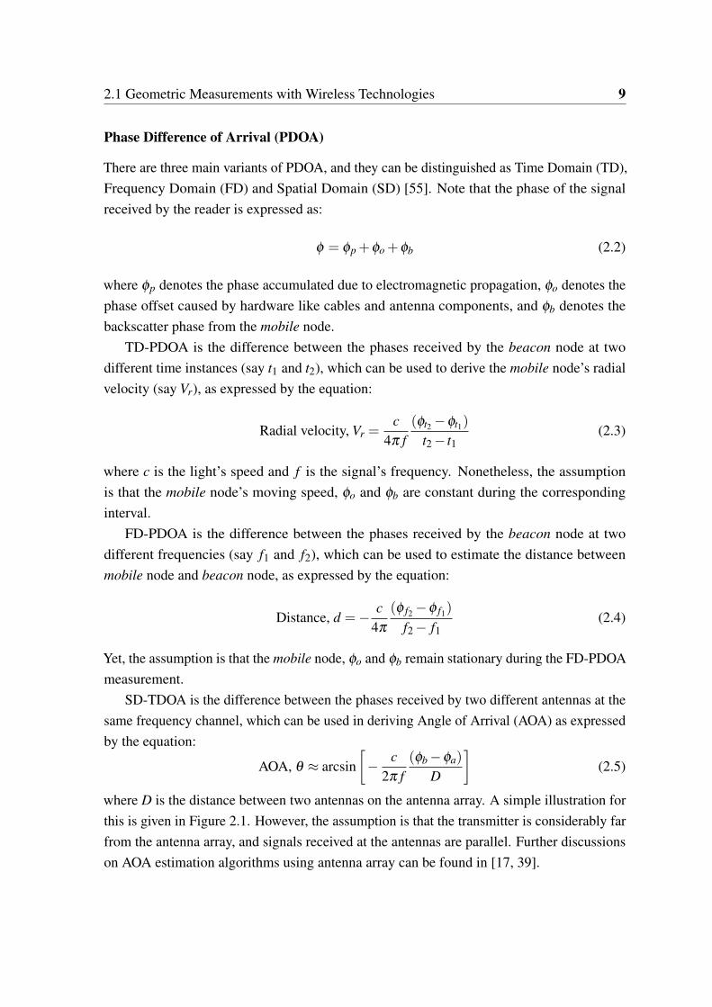
SD-TDOA is the difference between the phases received by two different antennas at thesame frequency channel, which can be used in deriving Angle of Arrival (AOA) as expressedby the equation:
AOA, θ ≈ arcsin[− c
2π f(φb−φa)
D
](2.5)
where D is the distance between two antennas on the antenna array. A simple illustration forthis is given in Figure 2.1. However, the assumption is that the transmitter is considerably farfrom the antenna array, and signals received at the antennas are parallel. Further discussionson AOA estimation algorithms using antenna array can be found in [17, 39].

10 BackgroundSD-PDOA
D
𝜃
Signal
Antenna
Transmitter
Fig. 2.1 Derivation of AOA from SD-TDOA.
Received Signal Strength Indicator (RSSI)
RSSI is a measure of power still present in the propagated radio wave when it is detectedby a receiver. The RSSI value is typically represented in dBm, on a scale particular tothe hardware chip-set. Greater RSSI value means shorter distance between transmitter andreceiver. Several theoretical and empirical models [50, 58, 65, 67] could be used to expressthe correlation between RSSI and distance, and one of popular ones is shown below:
R = β −10n log10 d + ε (2.6)
where R denotes the RSSI obtained at distance d, β denotes the RSSI measured at a referencedistance which is usually 1 meter from the transmitter, n denotes the path loss exponentwhich typically ranges from 2 to 6 for indoor environments, and ε denotes a Gaussian randomvariable with zero mean and standard deviation σrssi. However, as the models assume thatRSSI varies logarithmically with increasing distance in any directions from the source, theirreliability are limited especially in indoor environments due to Non-Line-Of-Sight (NLOS)conditions as well as other factors like hardware specifications (e.g. chipset and antenna) andantenna’s orientation.

2.2 Conventional Positioning Techniques 11
2.2 Conventional Positioning Techniques
Proximity
This technique localizes the mobile node simply by binary connectivity between the mobilenode and the beacon node. The beacon nodes are usually uniformly distributed over thearea of interest. When the mobile node senses a beacon node via wireless communication,it is considered to be within the transmission range of corresponding beacon node. In casewhen two or more beacon nodes are detected simultaneously, only the one which contributesthe strongest signal strengths shall be referred. However, the technique’s limitation is thatit tells not the absolute position (i.e. coordinates) but relative whereabouts of mobile node.For example, Cell Identification or Cell of Origin (COO) is a real-life application of thistechnique that tells which zone the cellular telephone lies within by identifying its associatedcell tower. For indoor scenarios, the estimation resolution can be improved by covering thesite of interest with higher density of beacon nodes which are preferably low-cost such asRFID tags [9].
Lateration
The concept of this technique is to deduce the mobile node’s position by knowing how far itis apart from the reference node. The separation distance can be derived from measurementslike RSSI, TOA, TDOA, RTT and PDOA. With single separation distance known, the node’sposition may be any point on the circle of the corresponding reference node as illustrated inFigure 2.2.
d1
Beacon node
Mobile node’s actual position
Mobile node’s likely position
Lateration
Fig. 2.2 Illustration: Lateration
For 2-dimensional positioning, as illustrated in Figure 2.3, three separation distances aretypically used to find the intersection which signifies the mobile node’s likely position, and

12 Background
such procedure is particularly known as Tri-Lateration. Note that circles shall be replacedby hyperbolas when separation distances are derived from TDOAs, and the reference nodesmust be non-collinear and non-collocated. When more than three separation distancesare considered, 3-dimensional positioning is made possible and the procedure is calledMulti-Lateration instead. In reality, the intersection is likely to happen at multiple points ormay not happen at all, due to wave phenomena like multipath and absorption that result inpoorly estimated separation distances. Therefore, the absolute position is usually finalized byfinding one exact point which fulfills all the measured separation distances simultaneously ina Least-Squares sense [37, 62]. The estimation accuracy improves when more separationdistances get taken into consideration. GPS technology is one prominent example thatemploys Multi-Lateration with TOA or TDOA -based distance measurements [70].
d1
d2
d3
Tri-Lateration
Beacon node
Mobile node’s actual position
Mobile node’s likely position
Fig. 2.3 Illustration: Tri-Lateration

2.2 Conventional Positioning Techniques 13
Triangulation
An AOA only implies that the mobile node may lies on anywhere along the line heading in thatspecific direction from the reference, as depicted in Figure 2.4. However, the use of two AOAsat a time enables one to pinpoint the mobile node’s 2-dimensional location. As illustratedin Figure 2.5, a triangle can be visualized by an intersection of two AOAs from differentreference nodes whose positions are known; hence, the mobile node’s can be deduced byfinding the missing sides and angles of the triangle (based on trigonometry). Such procedureis known as Triangulation, otherwise called Multiangulation when more than two AOAs areconsidered during the computation. [68]. The latter enables 3-dimensional positioning. MoreAOAs considered means better estimation accuracy. However, the drawback of this techniqueis its complexity and deployment cost due to the use of directional antennas or antenna arraysfor AOA measurements [4, 46]. Nevertheless, both Triangulation and Multiangulation have along history in robot localization, and a summary of their diverse algorithms can be found in[59].
𝜃1
AOA
Beacon node
Mobile node’s actual position
Mobile node’s likely position
Fig. 2.4 Illustration: Single AOA
𝜃1 𝜃2
known distance
Triangulation
Beacon node
Mobile node’s likely position
Fig. 2.5 Illustration: Triangulation

14 Background
Fingerprinting
The underlying concept of Fingerprinting (FP) is that each particular location within thesite of interest has a unique fingerprint. The fingerprint is actually a compilation of mea-surements which may be derived from radio signals (e.g.RSSI) from surrounding beaconnodes, magnetic field[10, 16, 60] and any other information that are location-dependent.Specifically, the procedure of Fingerprinting consists of two phases: offline phase and onlinephase. The offline phase serves to prepare the database prior to the online phase. In doingso, the site of interest is first divided into sub-areas and each sub-area is represented by aReference Point (RP). At each RP, signals from deployed beacon nodes or related sensorsare sampled multiple times in compiling a fingerprint. All fingerprints are then stored in adatabase along with position coordinates of their corresponding RPs. In the online phase, thereal-time measurements by mobile node are used to perform matching with the fingerprintsexisting in the database, and hence coordinates of RP whose fingerprint yields the closestmatch shall be the estimated position of mobile node. Some typical matching algorithmsare k-Nearest Neighbour (KNN), probabilistic methods, neural network, Support VectorMachine (SVM) and smallest M-vertex polygon (SMP) [47]. More details on a variety of FPmethods can be found in [54].
Besides employing the right matching algorithm, the estimation accuracy improves bydistributing more RPs over the site of interest. More RPs means each RP’s denoted areashrinks. However, the problem is that sometimes the measurements obtained at some RPsmight be very similar thereby causing their fingerprints hardly distinguishable. Therefore,the allocation of RPs must be carefully done for optimal precision. Given a fixed amountof RPs, FP’s reliability can be improved by taking more beacon nodes into consideration[7, 30]. Though FP is well known for having high resilience towards NLOS conditions, themajor downside is its laborious and time-consuming site-survey for database start-up as wellas maintenance which is necessary to account for any changes made to the environment (e.g.addition/removal of beacon nodes or walls). Even so, FP has been popular among the Wi-Fibased IPS [25].

2.2 Conventional Positioning Techniques 15
Dead-Reckoning
Unlike all the aforementioned positioning techniques, Dead Reckoning (DR) is a self-contained solution that requires no beacon nodes but only a single device like InertialMeasurement Unit (IMU) which contains all the related sensors to be carried by mobile node.The current position of mobile node is estimated by projecting forward its previous positionwith known distance and heading. For 2-D scenario, the mobile node’s position P at time tcan be simply computed by:
Pt = [Xt Yt ]⊺ (2.7a)
Xt = Xt−1 +D.cos(θt) (2.7b)
Yt = Yt−1 +D.sin(θt) (2.7c)
where X and Y denote coordinates in two dimensional space, θ is the heading and D is thedistance traveled within the time interval. The very beginning position and heading of mobilenode are often assumed known. Ideally, the consecutive positions can always be derivedby knowing the distance traveled and heading at following time intervals. There are twoways to find the distance traveled: firstly, by double integration of successive accelerationmeasurements; secondly, by detecting the number of steps by observing certain patternswithin the sensor data; the length of each step is either assumed to be constant [15, 49, 71] ordependent on various parameters such as step frequency and acceleration variance [13, 43, 63].Specifically, DR that employs step detection in estimating the distance traveled is regardedas Pedestrian Dead-Reckoning (PDR). The heading is determined based on relative angulardisplacement [77] or absolute direction derived from either individual or fusion of readingsfrom sensors like accelerometers, gyroscopes and magnetometers. However, as the sensorsinherently suffer from non-zero and non-Gaussian noises, the resultant estimations are proneto accumulative errors thereby deteriorating DR’s reliability over time.

16 Background
2.3 Bayesian Filtering
The measurements taken by the sensors are never perfect, and so the estimates based onthem are bound to have random noises. Fortunately, if prior knowledge about the system’sdynamics and the involved sensors is available, then Bayesian Filtering [12] can be applied tomerge them with the additional measurements/observations from other sensors to probabilis-tically estimate the system’s states so that the error is minimized. In the context of indoorpositioning, oftentimes the state of interest is the position of tracked object and the system’sdynamics is how the object advances from its original positions to new ones based on everynew sequence of available measurements/observations. Kalman Filter and Particle Filter aretwo most commonly used Bayesian filters. Generally, the state-space model of the system isexpressed as follows:
xt = g(xt−1,ut−1,wt−1) (2.8)
zt = h(xt ,vt) (2.9)
where x is a vector representing the system’s state at time t; the function g(.) models thesystem’s dynamics; z is the measurement otherwise known as measured state; the functionh(.) maps the state to a measurement; u is the control vector; and w and v denote the state’snoise vector and measurement noise vector respectively.
Kalman Filtering
The Kalman Filter (KF) is a recursive means to optimally estimate the state of a lineardynamics system whereby the noises are Gaussian, so that the variance of estimation errorsis minimum. There are some variations of Kalman Filter that are specifically designedfor non-linear dynamics system, but consequently the variance of estimation errors hasbecome approximately minimum instead [69]. Among the variations, Unscented KalmanFilter (UKF) and Extended Kalman Filter (EKF) are two popular ones. Regardless, theprocedure of Kalman Filtering can be easily understood by firstly re-writing the model shownby Equation (2.8) and Equation (2.9) into a linear model as follows:
xt = Axt−1 +But−1 +wt−1 (2.10)
zt = Hxt + vt (2.11)

2.3 Bayesian Filtering 17
A, B and H are matrices; the process noise w and the measurement noise v are assumed inde-pendent of each other, and zero-mean Gaussian with covariance matrix Q and R respectively.
Once the KF model is defined, the KF algorithm that comprises two stages namely TimeUpdate and Measurement Update shall be iterated at every new time step or whenever newmeasurement zt is available. At every iteration, the stage Time Update comes first to obtain apriori estimates of the state x and the error covariance P at time t according to the equations
x−t = Axt−1 +But (2.12)
P−t = APt−1A⊺+Q (2.13)
where xt−1 and Pt−1 denote the a posteriori estimates of the state and error covariancerespectively at time t−1. The resultant a priori estimates namely x−t and P−t are then inputtedto the stage Measurement Update to generate the corresponding a posteriori estimates byusing the equations
Kt = P−t H⊺(HP−t H⊺+R)−1 (2.14)
xt = x−t +Kt(zt−Hx−t ) (2.15)
Pt = P−t −KtHP−t (2.16)
where K denotes the Kalman gain.If one thinks that the measurement z is more credible than the prediction (a priori estimate
x−), then the covariance matrix R should be decreased for greater Kalman gain K, and hencegreater credibility is given to z in computing the aposteriori estimate x. An example of theimplementation of KF in indoor positioning is presented in Chapter 3.4.4.

18 Background
Particle Filtering
In contrast to Kalman Filter, Particle Filter (PF) is the optimal state estimator for non-lineardynamics systems whereby the noises are non-Gaussian [24]. However, it requires relativelyhigher computational time, which may be undesirable in certain cases where real-timeestimates are needed. There are several variants of Particle Filter [5, 12], such as SamplingImportance Resampling (SIR) and Regularized Particle Filter (RPF). An example of SIRPF application is presented in Section 4.2.1. Despite the variants, the procedure of ParticleFiltering can be generally described in 5 sequential steps:
1. Initially, a finite set of particles is generated to represent possible estimates of state x.
2. All particles are propagated according to a predefined state model.
3. Each particle is assigned a weight based on its similarity to the inputted measurements.Higher similarity results in greater weight. All weights are normalized.
4. A new set of particles is generated by drawing particles from existing set of particlesin proportion to their assigned weights.
5. Iteration commences from step no.2 at every new time step or whenever new measure-ment is available.
Basically, the concept behind PF is to use a finite set of independent random variablescalled particles to approximately represent the posterior probability for any complex model(which is probably non-Gaussian and multi-modal), and the posterior probability is evolvedwith new measurements according to Bayes’ theorem. An example of the implementation ofPF in indoor positioning is presented in Chapter 3.4.2

2.4 Related Work 19
2.4 Related Work
This work focuses on investigating ways that complement Pedestrian Dead-Reckoning (PDR)to achieve more reliable and robust indoor positioning. Therefore, this section documentsthe state of the art with respect to the PDR, besides summarizing some existing indoorpositioning methods which are related to the methods proposed in this work.
Pedestrian Dead-Reckoning
Generally, there are three core components in the PDR algorithm: step detection, step/stridelength estimation and heading determination. The most common way in detecting a stepis by observing peaks in acceleration signals. Some works have considered readings fromgyroscopes and magnetometers in detecting steps [33]. The gait cycle of a human is composedof two phases: Stance and Swing. Stance phase is when the foot flattens firmly on the groundwhile Swing phase is when the foot swings forward to enter its Stance phase. The heel-touching-ground event and heel-off-ground event that occur during transitions between thetwo phases can cause spikes in the vertical acceleration, and so a step can be identifiedby recognizing local minimum and/or local maximum within specifically sized slidingwindows [14, 81]. Regardless of the placement of the sensor/device, random jitters ormovements other than walking can contribute to unwanted acceleration peaks and hence thefalse steps. To validate the detected step, thresholds have been introduced to be comparedagainst various parameters such as the variance/standard deviation of accelerations withinthe sliding window [23, 57, 71], the magnitude difference between local maximum and localminimum [31, 35, 77], and the period between two consecutively detected steps [23, 41].As the gait cycles during normal walking are fairly consistent, similar waveforms can beobserved from sensor data. By measuring the similarities among the waveforms usingtechniques like Dynamic Time Warping (DTW) and Auto-correlation, the occurrence ofstep can thus be inferred [24, 44, 61]. For more robust detection of steps, classifiers aredeveloped to distinguish the pedestrian’s motion modes like walking, standing still andirregular movements based on a set of features extracted from sensor data [23, 73].
Once a step is identified, its length is important to indicate the distance traveled. Theactual length of a step varies from person to person depending on factors like leg’s length andwalking speed. Persons that have longer legs tend to have bigger step length. Besides, biggerstep length is also usually observed from higher walking speed. To walk faster, naturallythe person increases the frequency of their gait cycle, and while doing so some body partslike hip and foot may experience sharper changes in acceleration. Therefore, models thatrelate the step length with frequency [23, 44, 57] or acceleration [31–33, 36, 79] have been
20 Background
attempted for online estimation of step length for different walking patterns. Nonetheless,if the pedestrian walks normally at constant pace, implementing fixed step length for allthe detected steps throughout the walk is deemed a viable, not to mention computationallymuch simpler, alternative because the variance of each step under such condition seems to benegligible [8, 71]. Fixed step length can be predetermined either through trials [15, 49, 71]or based on individual height and weight [14, 77, 81].
Aside from the inaccurately estimated distance traveled, erroneous heading has beenreported as the dominant source of positioning errors in PDR based systems [1, 23, 31, 33,41, 49, 71]. Basically, the heading is derived based on readings from sensors i.e. gyroscopes,accelerometers and magnetometers. Single integration of gyroscopes’ readings gives an-gular displacement of the device while the digital compass composed of either individualmagnetometers or fusion of accelerometers and magnetometers tells the device’s absoluteorientation i.e. azimuth. The device’s orientation is not necessarily the pedestrian’s headingas it is dependent on its placement on pedestrian e.g. in pocket or in swinging hand. If thedevice’s orientation is aligned with pedestrian’s heading, azimuth values are typically usedto denote the pedestrian’s headings [14, 23, 29, 33, 35, 81]. Otherwise, the very beginningheading of the pedestrian and/or device’s orientation must be known beforehand so that theangular displacements computed using gyroscope or compass can be useful to deduce laterheadings [31, 41]. Either way, the estimated headings are bound to have errors because thecompass is susceptible to unpredictable magnetic disturbances at times and the gyroscope’accuracy drifts over time [1]. The coupling of both compass and gyroscope however, ascompared to each individual sensor, is able to achieve more reliable heading estimation[15, 23, 32, 40, 44, 49, 77, 83]. The common idea is to compare both compass and gyroscopedata as an effort to mitigate the magnetic fluctuations or gyroscope’s inherent biases, andhence fuse the data accordingly using techniques like Kalman filtering [32, 83], Particlefiltering [44] and complementary filtering [15, 40, 49].
One popular means used in mitigating the sensor’s inherent bias as well as the driftthat results from integration of biased sensor data over time is called Zero-Velocity-Update(ZUPT) method. ZUPT method asserts that the foot is stationary at its Stance phase wherebyits acceleration and velocity are supposedly zero. So, any non-zero accelerations andvelocities that exist during Stance phase are considered errors and thus be reset to zero.Reliable detection of Stance phase from pedestrian’s gait cycle is crucial to the effectivenessof ZUPT method. Therefore, the relevant sensors are usually mounted on the foot [2, 19, 33,48, 83] because the movement of foot, as compared to that of other body parts, gives moreapparent hints of gait cycles while walking.

2.4 Related Work 21
Various schemes have also been attempted to complement PDR by making use of externalor additional information. Some works like [41, 44, 57, 61] assume that the indoor map orfloor plan is available and so information like constraints and paths can be retrieved from themap to rectify the estimated trajectory and heading. The corrections of estimated trajectoryand heading in [77] are triggered upon detecting a virtual landmark. Virtual landmarks areidentified by observing distinct signatures/patterns in the data extracted from magnetic andinertial sensors as well as Wi-Fi signals – for instance, overhearing a unique set of Wi-Fiaccess points at a particular corridor-turn. The actual location of each virtual landmark,however, is derived by repetitive estimation via PDR expecting the outcome would eventuallyconverge to its actual location. In [23], besides having aids from Global Positioning System(GPS), map matching is triggered upon detection of certain patterns in user’s movementbased on accelerometers’ reading. E.g. if the detected pattern is recognized as “using anelevator”, the nearest elevator in vicinity is assumed as the user’s position. In [36], thepedestrian is assumed carrying at least two mobile devices and the relative displacementsof the devices with respect to the center of motion are reasonably stable as he/she walks.The devices individually estimate their own positions which is eventually corrected by acustomized Maximum A Posteriori estimation. RSSI-based distance measurements derivedfrom perceived wireless signals such as Ultrasound and Wi-Fi are used to complement PDRin [15, 35, 49]. Certainly, the use of Bayesian filter like Kalman filter (KF) [69] and Particlefilter (PF) [5] is not uncommon among the existing works in fusing the available data and/orestimates for more optimal estimation. In general, better positioning performance is assuredwhen more information is taken into consideration.
Collaborative Positioning
Another emerging means to gather more information for better position estimation is byutilizing the collaboration among the pedestrians to share the information among them-selves. Collaborative positioning method is made possible due to the existence of clusters ofpedestrians (who carry smart-devices) which is common in crowded places like mega-malls,universities and airports. The information shared among the pedestrians for collaborativepositioning/navigation purposes can be of any types e.g. their relative/absolute positionestimates and sensors’ readings.
In [11], the FP-estimated position of a pedestrian is first corrected to a point where theresultant of forces exerted by nearby pedestrians is met. The force exerted by each nearbypedestrian corresponds to the confidence score which is computed based on the differencebetween its position estimated by FP and that of a PF. The corrected estimate is then fed intoanother PF to finalize the pedestrian’s estimated position.
22 Background
In [51], the pedestrians are expected to provide helpful feedback regarding their FP-estimated positions, which shall be used to update the database’s credibility, thereby improv-ing the subsequent FP estimates.
In [56], a group of pedestrians is assumed moving towards the same destination. Eachpedestrian is provided an RSSI map which serves to deduce a set of likely positions based onreal-time RSSI data. As the group moves, the set of likely positions shall be filtered accordingto their PDR-estimated trajectories, which eventually contains only a single estimate thatconcludes the group’s estimated position.
In [1], the magnetometer readings from multiple pedestrians that are deemed reliable bya machine learning algorithm are fused by using consensus algorithms for more refined PDR-estimated headings. However, the pedestrians are assumed moving in the same direction, andat least one of them must have uncorrupted magnetometer readings.
In [29], the crowd of pedestrian is first categorized into groups based on two factors: firstly,RSSI-based proximity among the pedestrians and secondly, similarity between pedestrians’PDR-estimated trajectories. The PDR-estimated trajectory of each pedestrian shall beadjusted to reasonably fit the average PDR-estimated trajectory of their group. The estimatedposition of each pedestrian in the group is then re-adjusted according to the resultant offorces caused by nearby pedestrians as well as the groups.
In [72], the differences between pedestrians’ PDR-estimated positions are constrained bya KF where the ranges derived from UWB signals are inputted as observations.
In [81], all the pedestrians share the same indoor map which has virtual grids on it. Thepedestrians exchange information among themselves, which happens only when the distancebetween them is short enough for their microphone to sense frequency peaks broadcastfrom nearby pedestrians. The information received is the location of the center of gridwhere nearby pedestrian’s PDR-estimated position lies in. The received locations are thenaveraged and fused with PDR-estimated position via a KF to finalize the estimated positionof pedestrian.
In [28], the pedestrian’s position is estimated using Ultrasound based Multi-Laterationwhere the references are beacon nodes and static nearby pedestrians.
In [31], PDR-estimated trajectory of the pedestrian is represented by a link structurewhere the links symbolize straight paths made by the pedestrian and the joints’ angles denotethe pedestrian’s headings. When a pedestrian detects any nearby pedestrians, the joints’angles of the involved pedestrians are re-estimated in a least-squares sense.
In [74], the FP-estimated positions of pedestrians are adjusted using a spring model whereestimated positions are represented as nodes and links/springs between the nodes have springconstants determined based on distance between nearby pedestrians as well as confidence

2.5 Summary 23
score of the FP estimates. The nodes get attracted or repulsed by the spring forces untilequilibrium state is achieved.
2.5 Summary
This chapter gives an overview of the fundamentals of indoor positioning by discussing themajor types of geometric measurements as well as the conventional positioning techniques.Besides, Kalman Filter and Particle Filter which are commonly used to fuse multiple typesof measurements/information for better estimates are briefly described. In addition, state ofthe art regarding PDR is documented. Lastly, some existing works that relate to the proposedmethods of this work are also summarized.


Chapter 3
Experimental Setup and Preliminaries
This chapter discusses about the preparation that is necessary prior to the evaluation ofproposed positioning methods which shall be presented in the following chapters.
3.1 Setup
Two different sites in Swinburne University of Technology Sarawak Campus as depictedin Figure 3.1, were used to evaluate the positioning performance of the proposed methods.Figure 3.2 and Figure 3.3 show partial area of site no.1 and site no.2 respectively. Duringthe experiments, the subject carried a Nexus 7 and walked along specific routes. All thenecessary data were retrieved from the Nexus 7 and then post-processed using a Matlabprogram to compute the subject’s positions.
Hardware
The hardware involved are listed as follows:
1. Asus Google Nexus 7 (version 2013)
2. "TP-Link Wireless N" Access Point (Model No.:TL-WA701ND) or Router (ModelNo.:TL-WR740N)
Their relevant specifications are shown in Table 3.1 and Table 3.2 respectively.

26 Experimental Setup and Preliminaries
Wi-Fi AP
Site no.1
Site no.2
Fig. 3.1 Plane view of test-sites

3.1 Setup 27
Fig. 3.2 Long corridor of site no.1.
Fig. 3.3 Open-plan office of site no.2.

28 Experimental Setup and Preliminaries
Table 3.1 Asus Google Nexus 7’s specifications
Operating System Android™ 4.3CPU Quad-core 1.5 GHzMemory 2GB RAMWLAN Wi-Fi 802.11 a/b/g/n, dual-bandSensor Accelerometer, gyro, proximity, compass
Table 3.2 Specifications of TP-Link Router/Access Point
Standards IEEE 802.11 b/g/nSignal rates Up to 150MbpsFrequency range 2.4 – 2.4835 GHzAntenna type 5dBi Omni-directional antennaTransmit power <20dBm (EIRP)Beacon interval 100ms
Data Collection
An Android app was developed and run on the Nexus 7 in order to retrieve the necessarydata (i.e. 3-axial linear accelerations, 3-axial angular rates, azimuth readings and RSSIvalues). The android app was written in Java using a software called Android DeveloperTools following the Application Program Interface (API) guides which are available from theofficial website of Android Developers. All types of data were captured at a sampling rate of50 Hz. Note that the actual refresh rate for RSSI measurements was approximately 1000ms.
Post-processing
The collected data were then inputted to a program written in Matlab. All types of collecteddata, except the azimuths, were filtered prior to the computation of subject’s positions.Specifically, a second-order low-pass Butterworth filter with 0.1 Hz cut-off frequency wasapplied onto RSSI data. The accelerometers’ readings were first processed via a movingaverage with a window size of 25, and subsequently a second-order low-pass Butterworthfilter with a cutoff frequency of 5 Hz. The gyroscopes’ readings were first processed viaa moving average with a window size of 25, and subsequently a second-order low-passButterworth filter with a cutoff frequency of 1 Hz.

3.2 RSSI-Distance Correlation 29
3.2 RSSI-Distance Correlation
There are two types of wireless signals considered in this work: Wi-Fi and Bluetooth. Foreither types of signals, the correlation between RSSI and distance can be expressed byEquation (2.6) whose parameters’ values are shown in Table 3.3. The employed path-lossmodel’s parameters’ values for Wi-Fi signal were approximated by finding the best-fit curve,as depicted in Figure 3.4 where each shaped spot denotes the average value of RSSI readingsacquired over a period of ten seconds from specific AP at random location within the site.The employed path-loss model’s parameters’ values for Bluetooth signal were adopted from[74]. Nonetheless, it is worth pointing out that derived values may be empirically adjusted.
Table 3.3 Employed path-loss model’s parameters’ values
Signal type n β
Wi-Fi 2.56 37.52Bluetooth 2.85 40.35
5 10 15 20
-65
-60
-55
-50
-45
-40
RSSI versus Distance
Distance (m)
RS
SI (
dBm
)
Average of 10 readings for AP1Average of 10 readings for AP2Average of 10 readings for AP3Average of 10 readings for AP4Best fit
Fig. 3.4 RSSI-Distance correlation at site no.2
From Figure 3.4, one can observe that the average RSSI values are considerably incon-sistent even at similar distances. This is inline with the common fact that RSSI readings

30 Experimental Setup and Preliminaries
are erratic, and hence the reliability of the path-loss models are limited as they assume thatthe RSSI varies logarithmically and isotropically from the transmitter. Other than signalinterference and NLOS conditions, the hardware itself is also one of the major factors thatcontribute to erratic RSSI values. The hardware may vary in terms of its chip-set as wellas antenna type. Besides, the RSSI readings are also influenced by antenna’s orientation[3, 20, 21, 75]. Nonetheless, the erratic RSSI data can be mitigated and made useful to acertain extent by empirically tuning the parameters of path-loss models or using appropriatefusion techniques along with some assumptions, as attempted in many existing works such as[15, 31, 42, 49, 52, 61, 74]. More sophisticated modelling of RSSI-distance correlation canbe found in [52]. Note that in this work, the distances estimated based on RSSI values via apath-loss model are simply rough estimates which shall then be utilized along with customfilters and techniques to contribute better positioning accuracy.

3.3 PDR Implementation 31
3.3 PDR Implementation
Conventional PDR is employed to estimate the pedestrian’s position on a per step basic byusing Equation (2.7). The pedestrian is assumed to be walking normally with the deviceheld either upright in hand or at waist level [15, 18, 64]. The assumption made is justifiablebecause it is intended in this work to demonstrate that, even under such optimisticallycontrolled condition, PDR suffers primarily from erroneous headings. Needless to say, worsecan be expected if PDR were to work under challenging conditions (e.g. irregular walkingpatterns and device placed in swinging hand/bag).
Step Detection
The length of each step is assumed fixed as the variance between each step’s length is verysmall when a person walks normally [71]. To detect the walking steps of the pedestrian, firstly,the norm of accelerations is computed from the raw 3-axis linear accelerations obtained fromthe smart-device:
Sarms [t] =
√a2
x [t]+ a2y [t]+ a2
z [t] (3.1)
Sarms is then processed by using a moving average filter with a window size of 25 to remove the
waveform’s mean value because only the variation in acceleration is needed. Subsequently asecond-order low-pass Butterworth filter with a cutoff-frequency of 5 Hz is applied to removethe high-frequency noise, thereby producing smoother and clearer waveform to ease theidentification of the peaks in the waveform. A step event is identified when there is a localmaximum followed by a local minimum in the waveform. Note that threshold is necessary inidentifying the local extrema among the computed norms of accelerations, and it is definedas 0.1 in this work. It is possible that the change in pedestrian’s heading may cause changein the magnitude of accelerations and hence result in undesired signal peaks, in other words,false step events. To avoid false step events, 3-axis angular velocities are used to computethe norm of angular velocities first,
Swrms [t] =
√w2
x [t]+ w2y [t]+ w2
z [t] (3.2)
then it is processed via a moving average filter with a window size of 25, and subsequently asecond-order low-pass Butterworth filter with a cutoff-frequency of 1 Hz. Then, any instanceof Sw
rms that falls within a certain range of magnitude is removed to further eliminate theunwanted noise so that the turn event can be easily identified. The turn event is recognizedby detecting a full cycle of sinusoidal-like waveform. So, any step event that occurs duringthe turn event will be ignored. An example of this phenomenon is illustrated in Figure 3.5.

32 Experimental Setup and Preliminaries
2800 3000 3200 3400
-5
0
5
Filtered Norm of Accelerations
Time instance
Mag
nitu
de
Step eventLocal maximumLocal minimum
2800 3000 3200 3400-200
-100
0
100
200Filtered Norm of Angular Velocities
Time instance
Mag
nitu
de
400Filtered Compass readings
Turn event Turn event
Fig. 3.5 Identifying the Step Event and the Turn Event.
Heading Estimation
The heading of the pedestrian ϑt can be obtained in two ways. The first way requires thepedestrian to hold the smart-device upright in hand so that the device’s orientation is inlinewith pedestrian’s actual heading, and hence their heading is simply computed by:
ϑt = θ (3.3)
where θ denotes the azimuth value which is extracted directly from smart-device via An-droid’s Application Program Interface (API). In contrast, the second way of acquiring ϑs, tis applied when the device’s orientation is unknown, and hence pedestrian’s heading isestimated by:
ϑt = ϑt−1 +∆θ (3.4)
where ∆θ is the change in azimuth during the turn event. However, it assumes that the deviceis attached at the waist level of pedestrian and the initial heading (ϑ0) is known. Figure 3.6shows an example on acquisition of ∆θ from the obtained azimuth values. Note that the

3.3 PDR Implementation 33
waveforms shown in Figure 3.6 are resulted from firstly a 220 degree anticlockwise rotationand subsequently a 120 degree clockwise rotation. According to the API guides providedby official website of Android Developers, the azimuth values are derived from fusions ofreadings of accelerometers and magnetometers. As accelerometers output bias will driftaccording to ambient temperature and magnetometers may experience magnetic disturbancesdue to ferromagnetic materials inside building, the derived azimuth values are bound to haveerrors. In addition, imprecise detection of the turn event may also result in erroneous ∆θ .
2800 3000 3200 3400
Time instance
Local minimum
2800 3000 3200 3400-200
-100
0
100
200Filtered Norm of Angular Velocities
Time instance
Mag
nitu
de
2800 3000 3200 34000
100
200
300
400Filtered Compass readings
Time instance
Azi
mut
h (d
eg)
Turn event Turn event
𝛥𝜃 𝛥𝜃
Fig. 3.6 Computing the change in Azimuth.

34 Experimental Setup and Preliminaries
3.4 Benchmarks
A number of some other positioning methods were prepared as benchmarks for the methodsproposed in this work, and they are listed as follows:
1. aTRI: RSSI -based Tri-Lateration
2. pSIR: Fusion of PDR and RSSI via Sampling Importance Resampling Particle Filter
3. pMCMC: Fusion of PDR and RSSI via Markov Chain Monte Carlo sampling
4. pKF: Fusion of PDR and Tri-Lateration via Kalman Filter
The selection of positioning methods for a fair comparison in terms of positioning perfor-mance is rather difficult as the existing methods are uniquely designed to work optimallywith specific requirements. For instance, the Fingerprinting or landmarks based methodscan be highly reliable only when the number of references is high which would requirelaborious and time-consuming site-surveys while some exploit external information likenearby pedestrians, indoor map and GPS. In short, better positioning performance comes withgreater requirement in several aspects like available information, hardware and preparationwork. The four existing methods listed above are chosen as benchmarks mainly because theycan be executed by using the same hardware involved in the proposed methods.

3.4 Benchmarks 35
3.4.1 Algorithm of aTRI
Adapted from [53], aTRI estimates the position of pedestrian by using RSSI-derived distancesfrom three Wi-Fi APs whose locations are assumed known. In cases where more than threeAPs are available, only APs whose RSSI values are top three highest among all are considered.
An iteration of aTRI algorithm is summarized by Algorithm 1 where t denotes the timeinstance; P is estimated position of pedestrian; and da, db, dc are the distances estimated viaa path-loss model based on the RSSI values obtained from three individual APs whose 2-dimensional Cartesian coordinates are represented by (xa, ya), (xb, yb) and (xc, yc) respectively.
Algorithm 1 An iteration of aTRI algorithm
1: A←((db,t)
2− (dc,t)2)− (
(xb)2− (xc)
2)− ((yb)
2− (yc)2)
2: B←((db,t)
2− (da,t)2)− (
(xb)2− (xa)
2)− ((yb)
2− (ya)2)
3: Ynum← B · (xc− xb)−A · (xa− xb)
4: Yden← (ya− yb)(xc− xb)− (yc− yb)(xa− xb)
5: Define Y-coordinate: Y ← Ynum ÷ Yden6: Xnum← A−Y · (yc− yb)
7: Xden← xc− xb
8: Define X-coordinate: X ← Xnum ÷ Xden9: Pt ←
[X Y
]⊺

36 Experimental Setup and Preliminaries
3.4.2 Algorithm of pSIR
pSIR uses a Sampling Importance Resampling (SIR) Particle Filter to combine PDR withRSSI-derived distance measurement. The use of SIR Particle Fitler in pSIR is very similar tothat of [35]. However, pSIR derives the distance via a path-loss model by using the RSSIdata, while [35] measures the distance based on propagation time of Ultrasound signals.The latter way of distance measurement is comparatively more reliable, but it can only beperformed when the Ultrasound emitter is less than few meters apart from the pedestrian;on the other hand, Wi-Fi signal can reach far longer distances, but pSIR utilizes only RSSIvalues that pass the RSSI threshold which is to be set empirically. Besides, unlike [35] thatconsiders only single distance at a time, pSIR may consider multiple distances at a time ifmultiple RSSI sources are seen. Having said that, this work simply assumes the positioningperformance of pSIR is equivalent to that of [35].
The pedestrian’s position is estimated on a per step basis. An iteration of pSIR algorithmis summarized by Algorithm 2 where t denotes the time instance; P equates
[X Y
]⊺ whereX and Y are the x- and y-coordinates of pedestrian; N is the sample size; S denotes a set ofsamples; L is the step length; ϑ is the PDR-estimated heading; εx and εy are random noiseswhich are zero-mean Gaussian; σr is the standard deviation of measurement noise; D denotesa set of distances between pedestrian and Wi-Fi APs whose RSSI values pass the desiredthreshold; and λ is the distance between the k-th sample and the n-th AP. Initial position (P0)is assumed known, and initial set of samples (S0) is generated from a Gaussian distribution(N (P0,σ)).
The procedure of Algorithm 2 can be summarized as follows:
1. (Lines no.1 to 10): A set of samples is generated to represent the likely positions ofpedestrian. The weight of each generated sample is then assigned based on D.
2. (Lines no.11 to 14): All samples’ weights are normalized.
3. (Lines no.15 to 28): A new set of samples is drawn from the previously generated setof samples, with probabilities proportional to their normalized weights.
4. (Line no.29): The mean of the new set of samples finalizes the estimated position ofpedestrian.

3.4 Benchmarks 37
Algorithm 2 An iteration of pSIR algorithm1: for k← 1,N do2: Generate a sample: S[k]t ← S[k]t−1 +L×
[cosϑt sinϑt
]⊺+[εx εy
]⊺3: Compute sample’s weight, w[k]
t :4: E← number of elements in D5: if E > 0 then6: w[k]
t ←∏En=1
(1√
2πσrexp
(− 1
2(σr)2 (D[n]−λ )2))
7: else8: w[k]
t ← 19: end if
10: end for11: Compute total weight: W ← ∑
Nn=1 w[n]
t12: for k← 1,N do13: Normalize sample’s weight: w[k]
t ← w[k]t ÷W
14: end for15: Initialize cumulative distribution function (CDF): c[1]← 016: for k← 2,N do17: Construct CDF: c[k] = c[k−1]+w[k]
18: end for19: Start at the bottom of CDF: m← 120: Draw a starting point: u[k]←∼N (0, 1
N )21: for k← 1,Ns do22: Move along CDF: u[k] = uk + 1
N (k−1)23: while uk > cm do24: m← m+125: end while26: Assign sample: S[k]t ← S[m]
t
27: Assign weight: w[k]t = 1
N28: end for29: Pt ← 1
N ∑Nl=1 S[l]t
38 Experimental Setup and Preliminaries
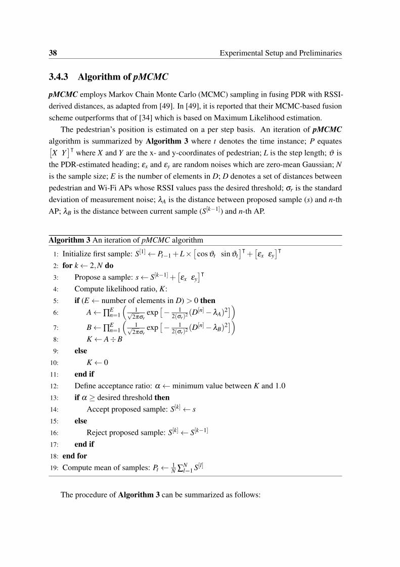
3.4.3 Algorithm of pMCMC
pMCMC employs Markov Chain Monte Carlo (MCMC) sampling in fusing PDR with RSSI-derived distances, as adapted from [49]. In [49], it is reported that their MCMC-based fusionscheme outperforms that of [34] which is based on Maximum Likelihood estimation.
The pedestrian’s position is estimated on a per step basis. An iteration of pMCMCalgorithm is summarized by Algorithm 3 where t denotes the time instance; P equates[X Y
]⊺ where X and Y are the x- and y-coordinates of pedestrian; L is the step length; ϑ isthe PDR-estimated heading; εx and εy are random noises which are zero-mean Gaussian; Nis the sample size; E is the number of elements in D; D denotes a set of distances betweenpedestrian and Wi-Fi APs whose RSSI values pass the desired threshold; σr is the standarddeviation of measurement noise; λA is the distance between proposed sample (s) and n-thAP; λB is the distance between current sample (S[k−1]) and n-th AP.
Algorithm 3 An iteration of pMCMC algorithm
1: Initialize first sample: S[1]← Pt−1 +L×[
cosϑt sinϑt]⊺
+[εx εy
]⊺2: for k← 2,N do3: Propose a sample: s← S[k−1]+
[εx εy
]⊺4: Compute likelihood ratio, K:5: if (E← number of elements in D) > 0 then6: A←∏
En=1
(1√
2πσrexp
[− 1
2(σr)2 (D[n]−λA)2])
7: B←∏En=1
(1√
2πσrexp
[− 1
2(σr)2 (D[n]−λB)2])
8: K← A÷B9: else
10: K← 011: end if12: Define acceptance ratio: α ← minimum value between K and 1.013: if α ≥ desired threshold then14: Accept proposed sample: S[k]← s15: else16: Reject proposed sample: S[k]← S[k−1]
17: end if18: end for19: Compute mean of samples: Pt ← 1
N ∑Nl=1 S[l]
The procedure of Algorithm 3 can be summarized as follows:

3.4 Benchmarks 39
1. The first element of the sample set (which comprises N number of elements) isinitialized based on a desired model, as detailed by line no.1.
2. A new sample is proposed by introducing random noise into the previous sample, asdetailed by line no.3.
3. The new sample is accepted as the next element of the sample set, only if the acceptanceratio is not smaller than certain threshold. Otherwise, the next element shall be thesame as the previous element. The acceptance ratio is computed as detailed by linesno.4 to 12.
4. Once all the elements of the sample set are computed, the mean of the sample setfinalizes the estimated position of pedestrian, as detailed by line no.19.

40 Experimental Setup and Preliminaries
3.4.4 Algorithm of pKF
Kalman Filter [69] has been employed to combine PDR with additional information likenearby pedestrians’ locations (in [81]) and GPS readings (in [23]). In this work, none of thoseadditional information but the RSSI data is available. Therefore, the RSSI data are used tocompute the pedestrian’s position via aTRI whose estimate is then inputted as measurementin the Kalman Filter to finalize the estimated position of pedestrian.
The pedestrian’s position is estimated on a per step basis. An iteration of pKF algorithmis summarized by Algorithm 4 where t denotes the time instance; P equates
[X Y
]⊺ whereX and Y are the x- and y-coordinates of pedestrian; L is the step length; ϑ denotes thePDR-estimated heading; A, B and H are 2× 2 identity matrices; both Q and R are 2× 2identity matrices multiplied by some appropriate scalars; z is pedestrian’s position estimatedsimultaneously by aTRI. The initial position of pedestrian (P0) is assumed known, and initialerror covariance (P0) equates Q. Note that lines no.5 to 9 in Algorithm 4 are standardequations for Kalman Filtering, as described in Chapter 2.3.
Algorithm 4 An iteration of pKF algorithm
1: Define control input: u← L×[
cosϑt sinϑt]⊺
2: if Pedestrian makes a turn then3: Reset error covariance: Pt ← Q4: end if5: Predict next state: x← A×Pt−1 +B×u6: Predict next covariance: Pt ← A×Pt−1×A⊺+Q7: Compute Kalman gain: K← Pt×H⊺ (H×Pt×H⊺+R)8: Update predicted state: x← x+K× (zt−H× x)9: Update predicted covariance: Pt ← Pt−K×H×Pt
10: Pt ← x
The procedure of Algorithm 4 can be summarized as follows:
1. The pedestrian’s next position (i.e. x) is first predicted by by projecting forward thepreviously estimated position (i.e. Pt−1) with known displacements, as detailed by lineno.5. The next covariance (i.e. Pt) is predicted by adding the current covariance (Pt−1)with some random noise (i.e. Q), as detailed by line no.6.
2. The Kalman gain (i.e. K) is computed based on some random noise (i.e. R), as detailedby line no.7. The Kalman gain shall be used to update both the predicted position andpredicted covariance, as detailed by lines no.8 to 9.

3.5 Summary 41
3. The updated x finalizes the estimated position of pedestrian.
3.5 Summary
Two different sites within the Swinburne University of Technology Sarawak Campus wereused for the evaluations of the positioning methods proposed in this work. The hardwarerequired were Nexus 7 tablets and Wi-Fi routers/access points. All the necessary data wereretrieved from the Nexus 7 via an Android app and then post processed by a Matlab programto estimate the subject’s locations. The path-loss model’s parameters’ values were defined bybest fitting the pre-collected RSSI data at known distances. Besides, the algorithms of PDRas well as some other PDR-based positioning methods adapted from existing works are alsoexplained in this chapter.


Chapter 4
Indoor Positioning by PedestrianDead-Reckoning with RSSI-basedschemes
As mentioned in Chapter 2.4, many efforts have already been made to enhance the posi-tioning performance of PDR by employing different techniques in processing the data fromPDR-related sensors data (i.e. accelerometers, gyroscopes and magnetometers), as well as bymaking use of additional but external information such as indoor map, GPS readings andnearby pedestrians’ data. In view of widespread Wi-Fi routers or access points in indoorenvironments, the RSSI of Wi-Fi signals has been favored by many researchers in developingindoor positioning methods especially those which are based on Fingerprinting. The Fin-gerprinting based methods are undoubtedly very promising, yet their relatively high setuprequirements are unfavorable.
This chapter presents two unique schemes that aim to aid smart-device -based PDR byutilizing the RSSI of Wi-Fi signals. The first scheme (detailed in Chapter 4.1) adjusts thePDR-estimated positions of pedestrian by detecting strong RSSI and subsequently requiringpedestrian’s manual input. Admittedly, the first scheme is not viable in situations whereuser intervention is not allowed. The second scheme (detailed in Chapter 4.2) rectifies thePDR’s dominant error source, i.e. erroneous heading, upon detecting long straight trajectoryin pedestrian’s motion.

44 Indoor Positioning by Pedestrian Dead-Reckoning with RSSI-based schemes
4.1 Position Correction Scheme
The procedure of position correction scheme is briefly shown in Figure 4.1. ConventionalPDR algorithm (detailed in Chapter 3.3) is employed to provide initial estimates for pedes-trian’s positions, assuming the pedestrian holds the smart-device upright in hand. Thecorrection on pedestrian’s estimated position is first executed upon observing strong RSSIfrom Wi-Fi APs. Alternatively, further correction may be triggered with manual input fromthe pedestrian. Such trigger is deemed reasonable in situations where pedestrian needs toreact accordingly to the system for further navigation guidance.
Ensure that the estimated position lies within acceptable region
Detect strong RSSI
Revise the estimated position based on compass bearing
Fig. 4.1 Flowchart of Position Correction Scheme.
4.1.1 Methodology
As the pedestrian walks, the RSSI readings obtained by the smart-device (held by pedestrian)from each visible APs are filtered and recorded as Rt,i, where i ∈ {1,2, · · · ,NA}, t denotes thetime instance and NA is the total number of visible APs. In the course of time, Rt,i is checkedagainst certain RSSI threshold Rth,i. The Rth,i corresponds to certain level of proximity(represented by dth,i) that exists between the estimated position Pt and ith AP. If
(Rt,i ≥ Rth,i
)is met, then
(dt,i ≤ dth,i
)is expected. The dt,i is the distance between the estimated position
Pt and ith AP, and it is computed by
dt,i =
√(Xt−Xi)
2 +(Yt−Yi)2 (4.1)
where Xi and Yi are the Cartesian coordinates of ith AP.

4.1 Position Correction Scheme 45
So, if(Rt,i ≥ Rth,i
)and
(dt,i ≤ dth,i
), then this Pt is within the “acceptable region” and
no further action is required. However, if(Rt,i ≥ Rth,i
)but
(dt,i ≥ dth,i
), then this Pt is not
accepted and shall be shifted radially towards the AP and subsequently relocated to a pointwhere
(dt,i ≤ dth,i
)is fulfilled. Such phenomenon can be illustrated by an example depicted
in Figure 4.2. Multiple acceptable regions can be assigned if the RSSI-distance relationshipis reliable over a longer distance, and would lead to more effective correction. Note thatthe RSSI value in reality does not vary isotropically from the RSSI source; regardless, thisscheme simply assumes the opposite.
c
A Acceptable region 1
Acceptable region 2
Wi-Fi AP
B C A
B
C
Actual position
Estimated position before correction
Estimated position after correction
Fig. 4.2 Position ‘B’ is not accepted and is therefore being shifted radially to Position ‘C’.
The estimated position can be further improved by utilizing the compass bearing (denotedas α i
t ) measured from ith AP to pedestrian. Whenever the condition(Rt,i ≥ Rth,i
)is detected,
the pedestrian is prompted to turn towards the corresponding AP and then trigger the systemto capture α i
t at that moment. Note that the APs should be placed in a way whereby they canbe spotted easily by the pedestrian. Admittedly, such scheme is only applicable in a controlledenvironment, e.g. museum; APs could be placed on top of certain displayed objects in themuseum, and so the visitors may approach an AP while viewing the displayed objects. Thesole purpose of having α i
t is to acquire vector displacement between pedestrian and AP.Subsequently, the pedestrian’s estimated position is finalized according to the acquired vectordisplacement, as illustrated by an example depicted in Figure 4.3 assuming that the capturedα i
t is 315◦ clockwise from North.
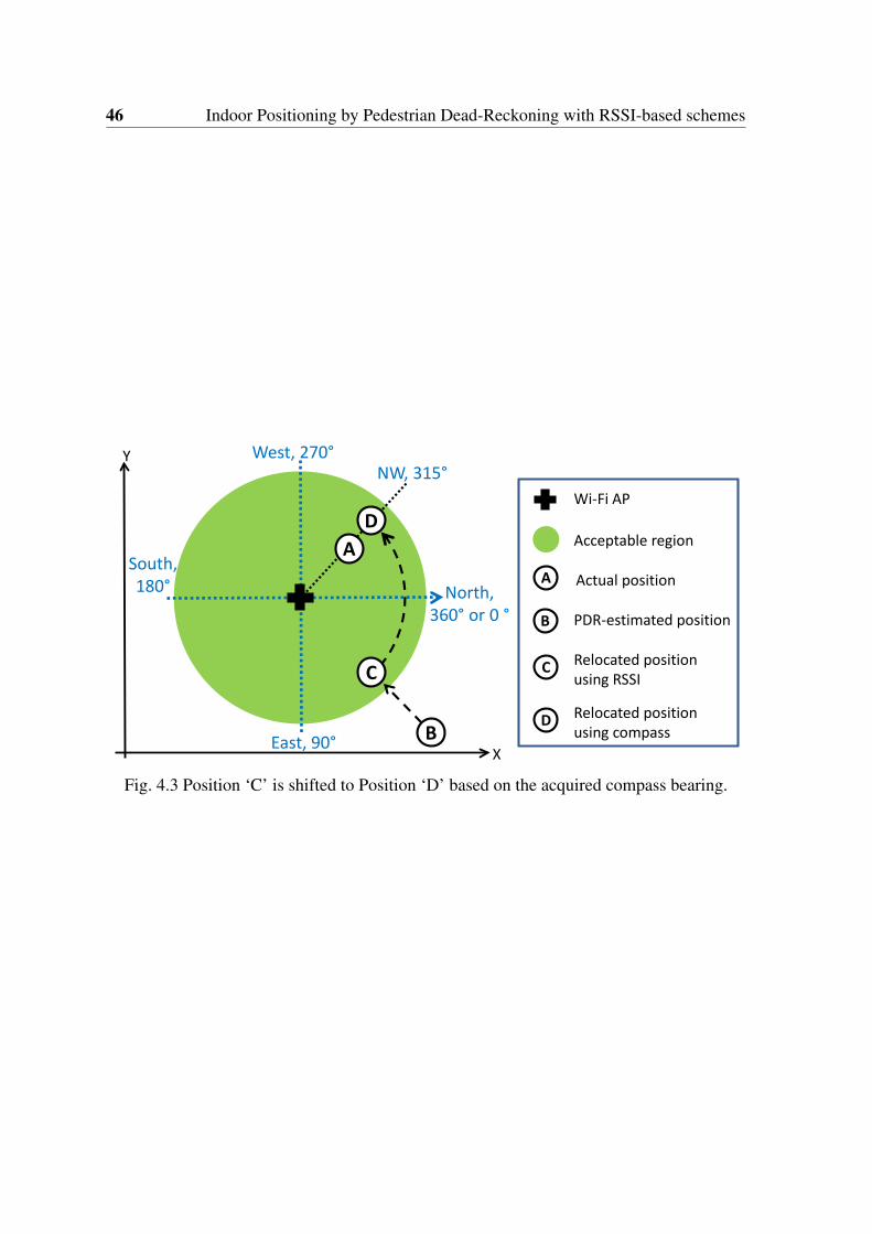
46 Indoor Positioning by Pedestrian Dead-Reckoning with RSSI-based schemes
West, 270°
East, 90° B
NW, 315°
C
D A
South, 180° North,
360° or 0 °
Y
X
c
Acceptable region
Wi-Fi AP
A
B
C
Actual position
PDR-estimated position
Relocated position using RSSI
D Relocated position using compass
Fig. 4.3 Position ‘C’ is shifted to Position ‘D’ based on the acquired compass bearing.

4.1 Position Correction Scheme 47
4.1.2 Evaluation
The proposed method had been tested in an open-plan office. A total of ten trials wereconducted. In each trial, the subject held a Nexus 7 upright in hand and walked along theroute beginning from ‘Start’ until ‘End’ as illustrated in Figure 4.4. Note that though thecondition
(Rt,i ≥ Rth,i
)may be fulfilled at any time along the route, the system was only
allowed to check whether condition(Rt,i ≥ Rth,i
)was achieved at checkpoints (i.e. ‘C4’,
‘C8’, ‘C10’ and ‘C13’.) only and to trigger correction accordingly. The RSSI-distancecorrelation of the site was considerably poor, as described in Chapter 3.2. In the experiment,two RSSI thresholds were employed and defined as −45 dBm and −50 dBm that correspondto 2 m and 5 m respectively, thereby resulting in two acceptable regions as indicated bydotted circles (with different radii) shown in Figure 4.4. The RSSI thresholds were selectednot to be smaller than −50 dBm because RSSI values lower than -50dBm were deemedrelatively unreliable, besides avoiding the acceptable regions of an AP from overlappingthose of another AP.
8 10 12 14 16 18 20 22 24 26 28 30 32
4
6
8
10
12
14
16
18
20
22
Coordinate X
Coo
rdin
ate
Y
AP3
AP1
AP2
AP4
C1C2
C3 C4
C5C6
C7C8C9
C10 C11
C12 C13Start
End
Fig. 4.4 Plane view of testbed.

48 Indoor Positioning by Pedestrian Dead-Reckoning with RSSI-based schemes
The proposed scheme is similar to those of [49], [35] and [15], in a sense that the pedes-trian’s PDR-estimated position is refined upon being in vicinity of beacon nodes. Specifically,Markov Chain Monte Carlo (MCMC) sampling is used in [49] to fuse PDR estimates withdistances derived from RSSI values which pass the threshold; Sampling Importance Resam-pling (SIR) Particle Filter (PF) is employed in [35] to combine PDR estimates with distancesderived from nearby (not more than few meters away from) ultrasound device; in [15], thepedestrian’s estimated position is directly assumed to be the position of beacon node whoseRSSI value is the highest and passes certain threshold. For comparison purposes, a total offive positioning methods were considered in estimating the subject’s positions, and they arelisted as follows:
1. pPDR: Sole PDR, as explained in Chapter 3.6.
2. pSIR: PDR with Sampling Importance Resampling, as detailed in Chapter 3.7.2
3. pMCMC: PDR with Markov Chain Monte Carlo sampling, as detailed in Chapter3.7.3.
4. pBN: Same as pPDR, but that the estimated position eventually gets replaced by theposition of Beacon Node whose RSSI value passes the threshold.
5. PM: Same as pPDR, but that the estimated position eventually gets adjusted by theproposed correction scheme.

4.1 Position Correction Scheme 49
Impact of varying number of deployed APs
The error metric is the absolute difference between estimated position and actual position.The lower the error, the higher the positioning accuracy. Figure 4.5 shows the errors of all thefive different methods when the number of deploys APs varied according to the arrangementsshown in Table 4.1. From Figure 4.5, it can be observed that mean error of PM graduallydecreases as the number of APs deployed increases, with lowest mean error of 1.4 m andstandard deviation of 1.8 m while pPDR’s are constantly 3.2 m and 1.8 m because PDR is notdependent on RSSI at all. Nonetheless, the improvement made on all methods except pPDRby increasing the number of deployed APs from 2 to 4 units seems insignificant becauseeven the biggest difference between corresponding mean error is just 0.6 m. This is probablyowing to the PDR component of PM that can estimate relatively accurate though for a shortduration. The accumulative error of PDR will eventually become significant, and that isexactly the time where the pedestrian needs to be close to the beacon nodes (i.e. APs) so thatstrong RSSI values may be available for all these RSSI-dependent methods (i.e. pMCMC,pSIR , pBN, PM) to execute appropriate correction. For example, as shown in Figure 4.6, theestimated route beginning from the ‘Start’ deviates progressively from actual route due tomere PDR with miscounted steps and primarily erroneous headings; once greatly improvedat checkpoint ‘C8’, the estimated route remains relatively close to the actual route all the wayfrom ‘C8’ until the ‘END’ with little improvement made at checkpoints ‘C12’ and ‘C13’;therefore, in this case, ‘AP2’ is deemed not as necessary as ‘AP4’. Nevertheless, as moreAPs are deployed along the route, there are more chances that the correction can be triggeredwhen necessary. Note that the estimated positions depicted in Fig. 4.6 are not mean values,but computed on a per step basis; when a step event occurs, the filtered RSSI value (whichis not lower than the selected RSSI threshold) at that instant only shall be considered inupdating the PDR-estimated position.

50 Indoor Positioning by Pedestrian Dead-Reckoning with RSSI-based schemes
Table 4.1 Arrangements of Wi-Fi APs considered during experiment
Arrangement No. Sources of RSSI considered
1 AP1, AP2, AP3, AP4
2 AP1, AP2, AP3
3 AP1, AP3, AP4
4 AP1, AP2, AP4
5 AP2, AP3, AP4
6 AP1, AP2
7 AP1, AP3
8 AP1, AP4
9 AP2, AP3
10 AP2, AP4
11 AP3, AP4
2 3 40
1
2
3
4
Number of APs deployed
Erro
r (m
)
pPDRpMCMCPMpSIRpBN
Fig. 4.5 Errors of different methods Versus Number of APs deployed

4.1 Position Correction Scheme 51
810
1214
1618
2022
2426
2830
3234
246810121416182022
Pla
ne v
iew
of T
estb
ed
Coo
rdin
ate
X
Coordinate Y
C1
C2C
3C
4
C5
C6
C7
C8
C9
C10
C11
C12
C13
C1
C2
C3
C4
C5
C6
C7
C8
C9
C10
C11
C12
C13AP
2
AP
4
Sta
rt
End
Act
ual r
oute
pMC
MC
pSIR
pBN
PM
pPD
R
Fig.
4.6
Atr
ial’s
resu
ltin
the
case
whe
reon
lytw
oA
Psw
ere
depl
oyed
.

52 Indoor Positioning by Pedestrian Dead-Reckoning with RSSI-based schemes
Impact of varying RSSI Threshold
The method PM had two RSSI thresholds set as−45 dBm and −50 dBm respectively whilethe remaining methods except pPDR had only one RSSI threshold set as −50 dBm. TheRSSI thresholds have to be empirically defined for optimal estimation. If RSSI threshold istoo high, correction is unlikely to happen unless the pedestrian is indeed near an AP to obtainsufficiently strong RSSI readings. If RSSI threshold is too low, correction gets triggeredunnecessarily and tends to fail because weak RSSI values are rather poor in implying thedistances between pedestrian and AP. Figure 4.7 and Figure 4.8 illustrate two examples ofoutcomes of faulty correction caused by erratic RSSI value or inappropriate RSSI threshold.In Figure 4.7, the condition
(Rt,i ≥ Rth,i
)was met and hence pedestrian turned towards ‘AP3’
and captured the α it (the bearing of pedestrian from ‘AP3’) to execute the proposed correction
scheme; however, as Rt,2 (RSSI from ‘AP2’) is greater than Rt,3 (RSSI from ‘AP3’) at thatmoment, PM mistakenly assumed the pedestrian was within the acceptable region of ‘AP2’instead of ‘AP3’ and therefore finalized the estimated position to a point where the bearingof estimated position from ‘AP2’ fulfilled the captured α i
t . In Figure 4.8, the Rt,2 (RSSI from‘AP2’) obtained by the pedestrian at checkpoint ‘C6’, which was supposedly lower than theRSSI threshold, unexpectedly passed the RSSI threshold and therefore led to faulty pBN.
Basically, both PM and pBN expect that the pedestrian’s closest AP gives highest RSSIvalue whenever the condition
(Rt,i ≥ Rth,i
)is met. In other words, the "acceptable region" of
an AP is not allowed to overlap with that of another AP. In contrast to them, the methodspMCMC and pSIR theoretically can make use of RSSI readings from any APs at a time.However, from Figure 4.9 that depicts the errors of pMCMC and pSIR for different RSSIthresholds, it is apparent that the −50 dBm was the optimal RSSI threshold for both pMCMCand pSIR in such test-site. Nonetheless, their errors are still worse than those of pBN andpPM, as shown in Figure 4.5. This thus infers that both the methods pMCMC and pSIRin the experiment ended up needing rather strong RSSI values (not lesser than −50 dBm),just like PM and pBN, but yielding comparatively lower positioning accuracy. Such poorperformance of both pMCMC and pSIR was probably caused by rather poor RSSI data,as their algorithms involve deriving the distances from RSSI values via certain path-lossmodel. From Figure 4.10 which shows the average absolute difference between RSSI-deriveddistances and actual distances at every checkpoint of the route, it is apparent that the RSSIdata obtained during the experiment are far from being reliable in deriving the distancesbetween pedestrian and APs. Note that RSSI-derived distances for all four APs were indeedcomputed via the same path-loss model.
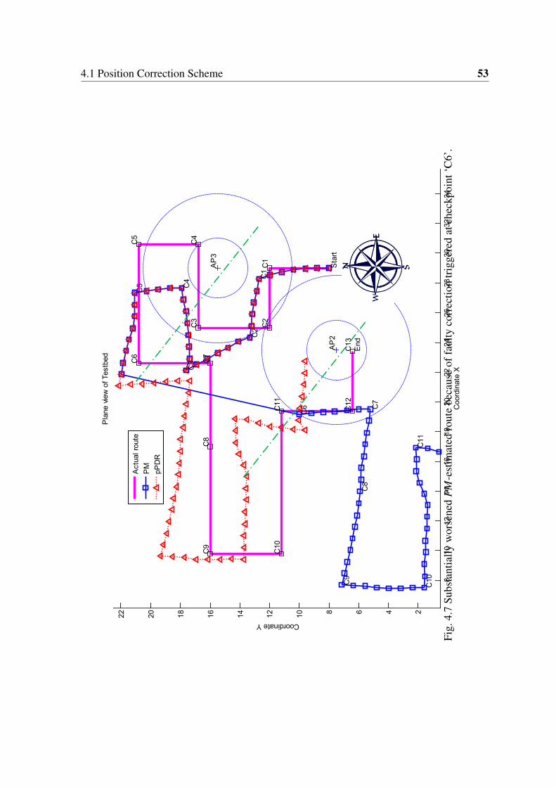
4.1 Position Correction Scheme 53
810
1214
1618
2022
2426
2830
3234
246810121416182022
Pla
ne v
iew
of T
estb
ed
Coo
rdin
ate
X
Coordinate Y
C1
C2
C3
C4
C5
C6 C
7C
8
C9
C10
C11
C1
C2
C3
C4
C5
C6
C7
C8
C9
C10
C11
C12
C13AP
2
AP
3
Sta
rt
End
Act
ual r
oute
PM
pPD
R
Fig.
4.7
Subs
tant
ially
wor
sene
dP
M-e
stim
ated
rout
ebe
caus
eof
faul
tyco
rrec
tion
trig
gere
dat
chec
kpoi
nt‘C
6’.

54 Indoor Positioning by Pedestrian Dead-Reckoning with RSSI-based schemes
1012
1416
1820
2224
2628
3032
34
2468101214161820
Pla
ne v
iew
of T
estb
ed
Coo
rdin
ate
X
Coordinate Y
C1
C2
C3
C4
C5
C6
C7
C8
C9
C10
C11 C12
C13
C1
C2
C3
C4
C5
C6
C7
C8
C9
C10
C11
C12
C13
AP
3
Sta
rt
End
Act
ual r
oute
pBN
pPD
R
Fig.
4.8
Subs
tant
ially
wor
sene
dpB
N-e
stim
ated
rout
ebe
caus
eof
faul
tyco
rrec
tion
trig
gere
dat
chec
kpoi
nt‘C
6’.

4.1 Position Correction Scheme 55
-60 -55 -50 -45 -402
2.5
3
3.5
4
4.5
RSSI threshold (dBm)
Erro
r (m
)
pMCMCpSIR
Fig. 4.9 Errors Versus RSSI threshold. (Case: Four APs deployed)
1 2 3 4 5 6 7 8 9 10 11 12 130
2
4
6
8
10
12
14
Checkpoint no.
Dis
tanc
e E
rror (
m)
RSSI of AP1RSSI of AP2RSSI of AP3RSSI of AP4
Fig. 4.10 Average absolute difference between RSSI-derived distances and actual distancesat all checkpoints along the route.

56 Indoor Positioning by Pedestrian Dead-Reckoning with RSSI-based schemes
Discussion
Admittedly, the fact that the pedestrian is required to manually trigger the system to capturethe compass bearing (α i
t ) in order to acquire vector displacement for correction purpose mayrender the proposed scheme not viable in applications where user intervention is prohibited.This scheme is not practical as it inconveniences the user to disrupt normal movementalong a desired walking path to aid error correction. Nevertheless, the scheme is for furtherimprovement and not the core technique itself. PM without vector displacement just simplyensures that the estimated position lies within the acceptable region, and when its acceptableregion is too small because of unreasonably high RSSI threshold, it becomes somewhatsimilar to pBN which outperformed both pMCMC and PM in the experiment anyway.
Regardless, this work intends to emphasize the importance of having vector displacementbetween pedestrian and AP, which is apparent especially in scenarios like the one shown inFigure 4.11. In Figure 4.11, the PDR-estimated route is way too much swayed from the actualroute that it falls into the northern region of ‘AP4’ when approaching ‘C8’; knowing onlyscalar displacements between pedestrian and ‘AP4’ can only shift the estimated positionstowards/outwards ‘AP4’ radially, just like how both pMCMC and pSIR do, and thereforethe resultant estimated positions still fall within the northern region of ‘AP4’; PM, whichknows the vector displacement between pedestrian and ‘AP4’, manages to shift the estimatedposition happening at ‘C8’ all the way from the North-East of ‘AP4’ to the South of ‘AP4’and the resultant estimated positions remain relatively closer to their actual positions.

4.1 Position Correction Scheme 57
810
1214
1618
2022
2426
2830
3234
246810121416182022
Pla
ne v
iew
of T
estb
ed
Coo
rdin
ate
X
Coordinate Y
C1
C2
C3
C4
C5
C6
C7
C8
C9
C10
C11
C12
C13
AP
4
Sta
rt
End
Act
ual r
oute
pMC
MC
pSIR
pBN
PM
pPD
R
Fig.
4.11
Atr
ial’s
resu
ltw
here
PM
cons
ider
ably
outp
erfo
rms
the
othe
rmet
hods
.

58 Indoor Positioning by Pedestrian Dead-Reckoning with RSSI-based schemes
4.2 Heading Correction Scheme
This scheme aims to correct the PDR-estimated headings ϑt by making use of the RSSIdata. Under this scheme, the pedestrian neither needs to approach any RSSI sources norprovides manual inputs. The correction of PDR-estimated headings, however, gets triggeredonly when the pedestrian’s movement constitutes a long straight trajectory. Such trigger isdeemed acceptable because long straight trajectory is commonly observed in pedestrian’sdaily movements, e.g. moving along long straight pathways in university, mega-mall, etc.The procedure of the heading correction scheme is briefly shown in Figure 4.12.
Estimate positions of the corresponding trajectory by making use of the RSSI data
Derive the heading based on Linear Regression
Detect a long straight trajectory
Update the pedestrian’s headings and positions
Fig. 4.12 Flowchart of Heading Correction Scheme.

4.2 Heading Correction Scheme 59
4.2.1 Methodology
Detection of long straight trajectory
A straight trajectory can be identified by observing a series of sequential positions estimatedby Equation (2.7), for instance (Pt ,Pt+1,Pt+2, · · ·) which occurs between the turn events.The size of the series implies the length of the straight trajectory. A straight trajectory isconsidered long only when its series’ size passes the threshold η . It is undeniable thatthe pedestrian’s trajectory across a long straight corridor/pathway may not be a completelystraight line at times. For example, slight deviation of course is performed to avoid bumpinginto another person who is moving along the same route. Even so, the straight trajectories ofthe pedestrian make before and after the course’s deviation can still be considered long iftheir corresponding series’ size passes the threshold η . The threshold η has to be empiricallydefined so that the detected straight trajectory is sufficiently long enough to enable a morereliable derivation of heading. Note that the detected long straight trajectory is termed asseries from now on.
Use of RSSI data for estimation of series’ positions
The RSSI data Ri during the time-frame of series are used to estimate their corresponding di
(which denotes the distance between pedestrian and i-th AP) based on a radio propagationmodel as follows:
Ri =−β −10n log10 di (4.2)
where β and n are predefined constants to fit the site’s RSSI-distance correlation [15, 74].A Sampling Importance Resampling (SIR) Particle Filter (PF) is employed to fuse PDR
estimates (i.e. steps and headings) with RSSI-derived distances di in estimating the positionsof the entire series. Optimal estimation can be achieved by fine tuning the filter’s parameters.Map information is commonly used in a PF to restrict the estimated positions to fall onpathways instead of walls or obstacles [44, 57, 61]. However, in this work, indoor map isconsidered not available and thus only the derived distances di are inputted as measurementsto the particle filter.
Let It = [xt ,yt ]⊺ denote the position where xt and yt denote the coordinate x and y
respectively at time t. Given the initial position It−1, Ns samples of It are generated using theproposed motion model:
Ikt = Ik
t−1 +S× [cosϑt ,sinϑt ]⊺+[εx,εy]
⊺ (4.3)

60 Indoor Positioning by Pedestrian Dead-Reckoning with RSSI-based schemes
where k = 1, . . . ,Ns and S is the step’s length. Both εx and εy are ∼N (0,σq2) where σq
is the standard deviation of the process noise. The weight of each generated sample, wk iscomputed by:
wk =
∏NAi=1
1√2πσr
exp[− (di−gk
i )2
2(σr)2
]if NA ≥ 1
1 if NA = 0(4.4)
where σr is the standard deviation of the measurement noise. gki is the distance between
sample Ikt and i-th AP, computed by:
gki = ∥I
[k]t −Wi∥ (4.5)
where Wi denotes the location of i-th Wi-Fi AP which is assumed known. Then, the weightsare normalized:
wk =wk
∑Nsl=1 wl
(4.6)
Finally, Ns samples are drawn from the generated set of samples {Ikt }
Nsk=1 with probabilities
proportional to their w. With re-sampled set {Ikt }
Nsk=1, position It is simply the centroid of the
samples [35, 44]:
It =1Ns
Ns
∑k=1
Ikt (4.7)
Derivation of Heading based on Linear Regression
Once all the positions of the entire series (which is the detected long straight trajectory) arecomputed, a simple linear regression line is to be determined through these positions. Simplelinear regression is a statistical method that models the relationships between a dependentvariable and an explanatory variable. As each position of the series has two variables namelyxt and yt , a right choice has to be made between regression of yt on xt and regression of xt
on yt .Consider a case where an object travels in a direction inclining to the horizontal axis rather
than to the vertical axis. In such case, one can infer that the object’s horizontal displacementis greater than its vertical displacement and hence regression of yt on xt is more appropriateto resemble the object’s direction. Likewise deduction can be applied for the opposite case.As for the series, the displacement made can be represented by the difference between theseries’ first and last positions as all the positions of series are sequentially estimated by a

4.2 Heading Correction Scheme 61
SIR PF. Let I f irst and Ilast denote the first and the last position of the series respectively. If∥x f irst−xlast∥ ≥ ∥y f irst−ylast∥, then regression of yt on xt is chosen. Otherwise, regressionof xt on yt is chosen. The orientation of the linear regression line is regarded as the newheading denoted as Θ. Admittedly, some estimated positions of the series could be outliersdue to erroneous RSSI readings. In this work, the outliers are indiscriminately consideredin deriving the new headings. The impact of the number of outliers on estimation accuracyshall be looked into in future work.
Finally, the pedestrian’s headings ϑ during the time-frame of the series are replacedby Θ. All the corresponding previously estimated positions Ps,t are re-estimated using(Equation (2.7)) with this newly updated ϑ . An example of such phenomenon is illustratedin Figure 4.13. Note that it is desirable to have longer series so that more estimated positionscan be considered to reliably derive the linear regression line.
Actual straight trajectory
Initial estimated trajectory
Re-estimated trajectory based on the orientation of the regression line
Regression line
series’ estimated positions
Fig. 4.13 The original headings of the PDR-estimated trajectory are updated to the orientationof the linear regression line. Hence, the estimated trajectory is re-estimated with updatedheadings.

62 Indoor Positioning by Pedestrian Dead-Reckoning with RSSI-based schemes
4.2.2 Evaluation
Figure 4.14 and Figure 4.15 depict the plan views of the sites which were used to evaluatethe efficacy of proposed heading correction scheme in improving the positioning accuracyof PDR. In terms of site’s area and no. of nodes deployed, the sites chosen are comparableto those of [15, 35, 42, 76]. Though not shown, the sites are fully equipped with machines,furniture as well as walls or barriers made of both glass and concrete. Furthermore, theexperiments were conducted during normal operating hours of the sites, which means a con-siderable number of students and relevant staff were present at the sites. All these obstaclesand disturbances present at the sites undoubtedly contribute to erratic RSSI measurements.The purpose of conducting the experiments in such scenario is to test the robustness of theproposed method towards erratic RSSI values.
18 23 28 33 38 43 48 53 5812
17
22
27
32
37
42
Coordinate X
Coo
rdin
ate
Y
AP1 AP2
AP3AP4
Start
End
T1
T2T3
T4 T5
T6 T7
T8T9
T10
Route A
Fig. 4.14 Plane view of test-site no.1.
A total of ten trials were conducted. In each trial, the subject held a Nexus 7 at theirwaist and walked normally along the route, as illustrated in Figure 4.14 and Figure 4.15

4.2 Heading Correction Scheme 63
6 8 10 12 14 16 18 20 22 24 26 28 30 322
4
6
8
10
12
14
16
18
20
22
Coordinate X
Coo
rdin
ate
Y
AP3
AP1
AP2
AP4
Start
End
T1
T2Route B
Fig. 4.15 Plane view of test-site no.2.
respectively, beginning from ‘Start’ until ‘End’. The ‘T1, T2, . . . T10’ indicate the positionswhere the pedestrian changed its heading. Note that some pauses and minor path deviationsdid occur because the pedestrians had to open doors as well as avoid bumping into otherpersons while walking along the same pathways. Nevertheless, subject was asked to followthe designated routes as closely as possible so that the occurrence of imprecise distancetraveled can be minimized and impact of erroneous heading onto PDR’s performance canbe apparently observed. The primary purpose of having the routes designated so was to testthe viability of the RSSI based heading correction and hence examine the improvement itcould bring to the conventional PDR. Table 4.2 and Table 4.3 tabulate the correspondingroute’s straight paths and the actual number of steps performed in each path. Nonetheless,slightly miscounted number of steps is inevitable due to inaccurate step detection based onnoisy inertial data. The ground-truth was determined by marking the time-stamp of everynew position along the route.
The selection of positioning methods for a fair comparison in terms of positioning perfor-mance is rather difficult as the existing methods are uniquely designed to work optimally

64 Indoor Positioning by Pedestrian Dead-Reckoning with RSSI-based schemes
Table 4.2 Route A in test-site no.1
Path No. Segment of Route No. of steps taken
1 Start – T1 5
2 T1 – T2 3
3 T2 –– T3 6
4 T3 —- T4 9
5 T4 —- T5 7
6 T5 —- T6 12
7 T6 —- T7 30
8 T7 —- T8 12
9 T8 —- T9 8
10 T9 –– T10 7
11 T10 – End 7
Table 4.3 Route B in test-site no.2
Path No. Segment of Route No. of steps taken
1 Start – T1 23
2 T1 – T2 6
3 T2 – End 23

4.2 Heading Correction Scheme 65
with specific requirements. For instance, the Fingerprinting or landmarks based methodscan be highly reliable only when the number of references is high which would requirelaborious and time-consuming site-surveys while some exploit external information likenearby pedestrians, indoor map and GPS. In short, better positioning performance comes withgreater requirement in several aspects like available information, hardware and preparationwork. The proposed method requires minimal information (i.e. RSSI, inertial and magneticmeasurements only) from the pedestrian’s device alone and no site survey. In this regard, theproposed method is similar to the ones proposed in [49] and [35]. For comparison purposes,a total of six positioning methods were considered in estimating the subject’s positionsthroughout the routes, and they are listed as follows:
1. pPDR: Sole PDR, as detailed in Chapter 3.6.
2. aTRI: Tri-Lateration based on RSSI, as detailed in Chapter 3.7.1.
3. pSIR: Fusion of PDR and RSSI via Sampling Importance Resampling Particle Filter,as detailed in Chapter 3.7.2.
4. pMCMC: Fusion of PDR and RSSI via Markov Chain Monte Carlo sampling, asdetailed in Chapter 3.7.3.
5. pKF: Fusion of PDR and Tri-Lateration via Kalman Filter, as detailed in Chapter3.7.4.
6. PM: pPDR with proposed heading correction scheme.
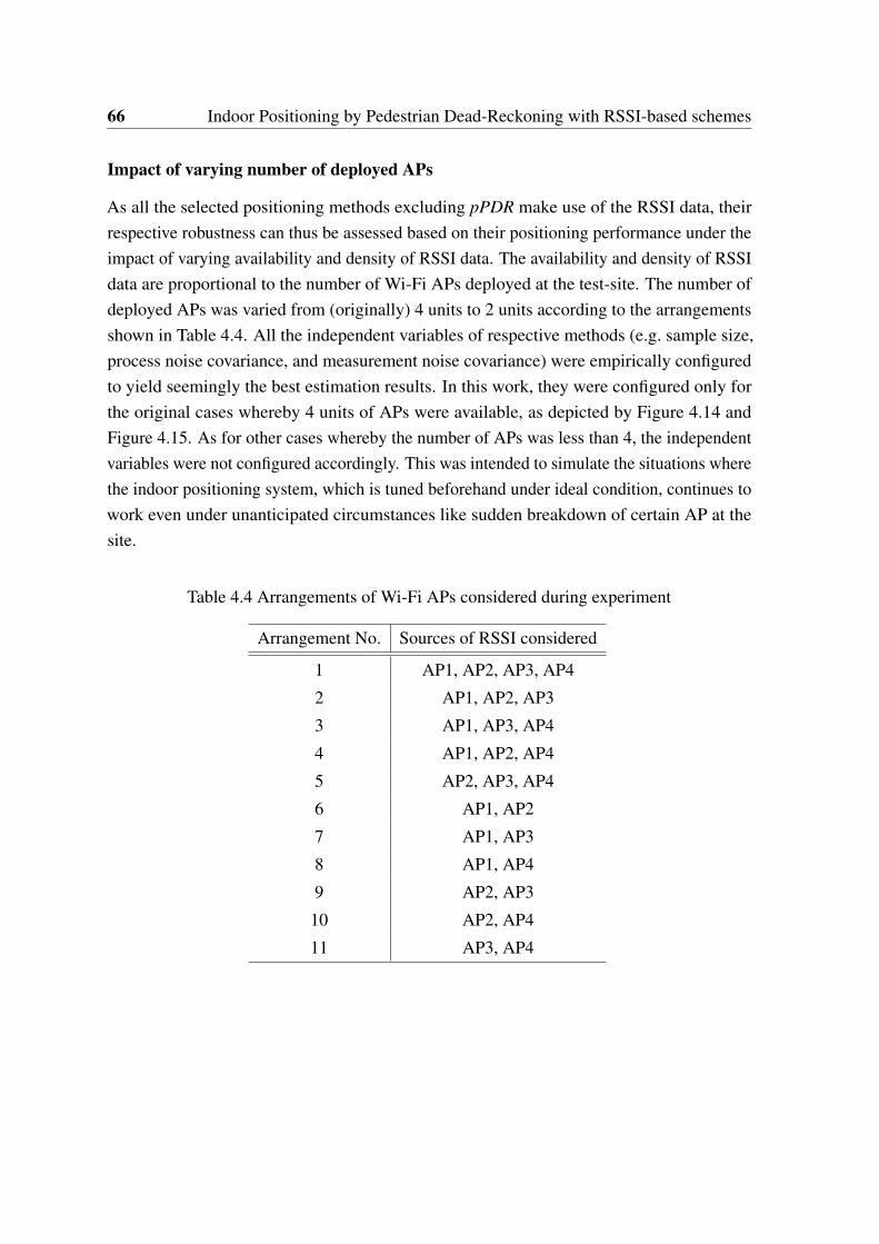
66 Indoor Positioning by Pedestrian Dead-Reckoning with RSSI-based schemes
Impact of varying number of deployed APs
As all the selected positioning methods excluding pPDR make use of the RSSI data, theirrespective robustness can thus be assessed based on their positioning performance under theimpact of varying availability and density of RSSI data. The availability and density of RSSIdata are proportional to the number of Wi-Fi APs deployed at the test-site. The number ofdeployed APs was varied from (originally) 4 units to 2 units according to the arrangementsshown in Table 4.4. All the independent variables of respective methods (e.g. sample size,process noise covariance, and measurement noise covariance) were empirically configuredto yield seemingly the best estimation results. In this work, they were configured only forthe original cases whereby 4 units of APs were available, as depicted by Figure 4.14 andFigure 4.15. As for other cases whereby the number of APs was less than 4, the independentvariables were not configured accordingly. This was intended to simulate the situations wherethe indoor positioning system, which is tuned beforehand under ideal condition, continues towork even under unanticipated circumstances like sudden breakdown of certain AP at thesite.
Table 4.4 Arrangements of Wi-Fi APs considered during experiment
Arrangement No. Sources of RSSI considered
1 AP1, AP2, AP3, AP4
2 AP1, AP2, AP3
3 AP1, AP3, AP4
4 AP1, AP2, AP4
5 AP2, AP3, AP4
6 AP1, AP2
7 AP1, AP3
8 AP1, AP4
9 AP2, AP3
10 AP2, AP4
11 AP3, AP4

4.2 Heading Correction Scheme 67
2 3 4
2
4
6
8
10
12
No. of APs deployed
Erro
r (m
)
pPDRPMpSIRpKFpMCMCaTRI
Fig. 4.16 Route A: Methods’ errors versus No. of APs deployed.
From both Figure 4.16 and Figure 4.17, one can be observe that: (i) While pPDR remainsunaffected as the number of APs decreases because it’s independent of RSSI data, theaccuracy of all the other methods deteriorates. From the steepness of change in averageerror when the number of APs decreases, it is apparent that the affected methods, arrangedin the order from highest to lowest degree of severity, are aTRI, pKF, pMCMC and lastlypSIR and PM. It is unsurprising that aTRI suffered the most from reduced number of APsbecause it relies on solely RSSI data, while other methods use both PDR and RSSI data tocomplement the estimation of pedestrian’s position. Recall that the outcomes of aTRI serveas measurements in pKF, therefore pKF’s deterioration rate is nearly as much as aTRI’s. Notethat aTRI requires RSSI readings from at least three APs, therefore its performance can’t betested in cases where only two APs are deployed. As for pMCMC and pSIR, apart from theirPDR component which is considerably reliable for short displacements, intakes of RSSI dataare also controlled whereby only the RSSI that passes the threshold Rth is used in calculatingthe distance. This therefore somewhat tells why they are not as significantly influenced byRSSI as aTRI and pKF are. Even so, pMCMC falls behind pSIR probably due to its MCMC

68 Indoor Positioning by Pedestrian Dead-Reckoning with RSSI-based schemes
2 3 40
2
4
6
8
No. of APs deployed
Erro
r (m
)
pPDRPMpSIRpKFpMCMCaTRI
Fig. 4.17 Route B: Methods’ errors versus No. of APs deployed.
sampling technique which, in comparison to SIR PF of pSIR, has higher demand for accurateRSSI data; otherwise poor or lack of RSSI data tends to cause indiscriminate acceptanceof many subsequently generated samples that will eventually result in the average of thegenerated samples to deviate unreasonably far from previous position estimate.
(ii) The performance of pPDR is rather good in case of route B that it surpasses allmethods except PM, as compared to its performance in the case of route A. One probableexplanation is that route B is less complicated than route A by having lesser turns and shortersum of distance traveled. Lesser turns made by pedestrian implies lower probability thatestimated heading ϑ gets jeopardized by imprecisely detected change in pedestrian’s heading∆θ . Shorter distance traveled along a straight path implies lesser amount of accumulated errorcaused by inaccurate ϑ as the pedestrian advances further. In addition, though inaccurate∆θ is undesired, sometimes it does accidentally result in correct ϑ . Figure 4.18 illustratesan example of such phenomenon. Therefore, it is safe to conclude that PDR’s reliabilityis unpredictable because the sensors’ inherent biases might neutralize the previous flawedestimations (i.e. distance traveled and heading) by chance. Being the primary key to steadily

4.2 Heading Correction Scheme 69
reliable PDR, the estimated heading ϑ needs to be corrected whenever necessary. However,the timing for heading correction is often not known without the aid of external referenceslike GPS and indoor map.
6 8 10 12 14 16 18 20 22 24 26 28 30
4
6
8
10
12
14
16
18
20
22Path no.3
Coordinate X
Coo
rdin
ate
Y
AP3
AP1
AP2
AP4
Start
End
ActualpPDR
Fig. 4.18 The inaccurately detected ∆θ , supposedly to be 90 degrees as equal to the actualchange in pedestrian’s heading at the last junction of the route, accidentally causes the ϑs tobe in line with the actual heading. Nonetheless, error in pedestrian’s estimated position Lshas been accumulated due to previous inaccurate headings.
(iii) PM outperforms all the other methods regardless of the number of APs deployed inboth cases, while being comparable with pPDR in case of route B. As previously mentioned,PM is actually pPDR with conditionally improved headings, thus it should portray anenhanced version of pPDR. The reason why PM is comparable with pPDR in the case ofroute B as shown in Figure 4.16 is that the PDR’s accuracy had not deteriorated until thestage where the heading correction can yield significant improvement. On the contrary, PMexcels in the case of route A (as shown in Figure 4.17) where pPDR has a 6.56 m mean errorwith 4.15 m standard deviation which is considerably worse than its 2.15 m mean error with1.28 m standard deviation achieved in the case of route B. By triggering heading correctionat single straight path namely path no.7 of route A, PM manages to improve PDR’s meanerror up to 49 %. PM’s performance can be more comprehensively demonstrated by itspropagation of average error over the route A, as shown in Figure 4.19 where the error is theabsolute difference between actual position and estimated position.

70 Indoor Positioning by Pedestrian Dead-Reckoning with RSSI-based schemes
111
2131
4151
6171
8191
101
0246810121416T1
T2T3
T4T5
T6T7
T8T9
T10
Sta
rtE
nd
Act
ual p
ositi
on n
o.
Error (m)
aTR
IpM
CM
CpK
FpS
IRP
MpP
DR
Fig.
4.19
Prop
agat
ion
ofav
erag
eer
roro
vert
hero
ute
A

4.2 Heading Correction Scheme 71
From Figure 4.19, it can be observed that, beginning from the ‘Start’, aTRI being theonly method which relies on solely RSSI data suffers immensely probably due to poorRSSI data while the deterioration of other methods is comparatively gradual because oftheir PDR component hence making them more resilient towards erratic RSSI data. As thevery beginning heading is given, PM being the pure PDR and unaffected by RSSI at earlystages like the pPDR has the slowest rate of deterioration as the pedestrian advances furtheralong the route. During the period between ‘T6’ and ‘T7’ however, considering aTRI’serror has been significantly improved, it seems that the RSSI data have become somewhatuseful to result in improvement on the accuracy of other RSSI-dependent methods whilepPDR’s error escalates primarily due to erroneous headings. Nonetheless, after ‘T7’, theRSSI-dependent methods’ accuracy fluctuates as the reliability of RSSI data does. UnlikepPDR, PM maintains its steady accuracy even after ‘T6’ because the interval between‘T6’and ’T7’ (i.e. path no.7) is where the new headings derived from orientation of regression linecome into effect. As a result of that, the pedestrian’s headings since then were also improved,as shown in Figure 4.20 which depicts the average discrepancies between actual headingsand estimated headings at each path of route A. For example, as shown in Figure 4.21a whichdepicts one of the experiment results, PM as well as pPDR gradually deviates from the actualroute due to mere PDR with miscounted steps and primarily erroneous heading; yet, afterthe heading ϑ at path no.7 gets aligned with the orientation of the regression line (which isdepicted in Figure 4.21b), PM remains comparatively close to the actual route.
2 3 4 5 6 7 8 9 10 110
5
10
15
20
25
30
35
40
Path no.
Ave
rage
hea
ding
erro
r (in
deg
ree)
pPDRPM
Fig. 4.20 Average heading error at each path of route A.
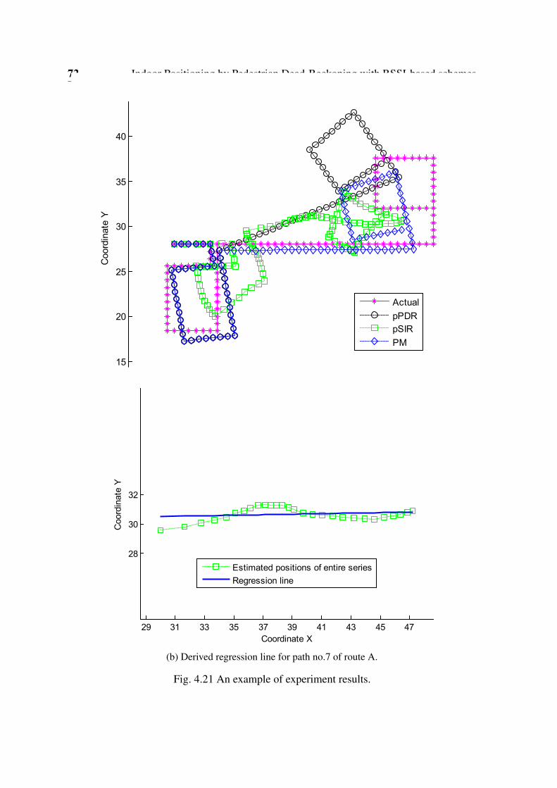
72 Indoor Positioning by Pedestrian Dead-Reckoning with RSSI-based schemes
20 25 30 35 40 45 50
15
20
25
30
35
40
Coordinate X
Coo
rdin
ate
Y
ActualpPDRpSIRPM
(a) Estimated route A by different methods.
29 31 33 35 37 39 41 43 45 47
28
30
32
Coordinate X
Coo
rdin
ate
Y
Estimated positions of entire seriesRegression line
(b) Derived regression line for path no.7 of route A.
Fig. 4.21 An example of experiment results.

4.2 Heading Correction Scheme 73
Heading Derivation based on Linear Regression
Table 4.5 and Table 4.6 tabulate the average heading errors for Route A and Route Brespectively. The heading error is the scalar discrepancy between actual heading and headingderived based on linear regression (of series’ positions estimated by respective methods).Note that the actual headings were the true azimuths for the designated routes. From Table 4.5and Table 4.6, it is apparent that linear regression of series’ positions estimated by all methodsexcept pPDR result in average heading errors (highlighted in green) lower than those ofpPDR (highlighted in grey) especially when the path’s length is long. Recall that path no.7 isthe longest straight path of route A, and path no.1 and no.3 are among the longest straightpath of route B. As illustrated by a trial’s result shown in Figure 4.22, the route estimated byaTRI itself seemingly deviates far from the actual route, yet the regression lines somewhatresemble the true headings of route B. Some additional results are depicted in Figure 4.23.Nonetheless, the accuracy of such heading derivation approach deteriorates as the numberof the APs decreases. Even so, the statistics shown have demonstrated that, in occasionof long straight path, this technique may be feasible as an alternative to the conventionalheading estimator of PDR. Note that this scheme is basically PDR with conditional headingcorrection; PDR is primarily used to estimate the positions of the pedestrian as he/she walks;correction of estimated heading occurs only when a long straight trajectory is identified;Figures 4.18, 4.21, 4.22 and 4.23 apparently show that heading correction significantlyenhances the PDR-estimated positions.

74 Indoor Positioning by Pedestrian Dead-Reckoning with RSSI-based schemes
Table 4.5 Average scalar discrepancies between actual headings and headings derived basedon linear regression of series’ positions estimated by respective methods in the case of routeA. Note that the values highlighted in grey are the heading errors of PM when the headingcorrection is not applied; the values highlighted in green are smaller than those highlightedin grey.
.
Path No.Average Heading Error, (degree)
pPDR aTRI pKF pMCMC pSIR
2 7.9 40.0 18.1 38.6 29.13 6.3 8.1 6.9 21.4 7.44 9.8 52.1 12.1 32.7 8.35 8.7 94.9 32.0 84.7 46.76 12.9 75.0 23.6 50.8 24.57 27.4 2.8 6.8 7.3 3.18 35.6 46.3 55.4 54.9 58.69 33.4 92.5 52.6 91.5 77.4
10 30.3 141.0 39.9 126.9 65.511 28.6 28.5 32.9 12.7 44.4
(a) When No. of APs is 4
Path No.Average Heading Error, (degree)
pPDR aTRI pKF pMCMC pSIR
2 7.9 58.2 16.4 44.4 25.83 6.3 31.5 16.2 20.5 7.24 9.8 73.1 16.4 49.2 10.15 8.7 98.3 44.7 82.3 27.06 12.9 72.4 24.1 59.5 18.27 27.4 25.6 7.0 14.7 7.98 35.6 66.6 58.5 53.1 63.19 33.4 92.4 54.0 84.0 74.710 30.3 117.4 39.4 124.9 59.211 28.6 31.3 31.8 17.8 45.3
(b) When No. of APs is 3

4.2 Heading Correction Scheme 75
Table 4.6 Average scalar discrepancies between actual headings and headings derived basedon linear regression of series’ positions estimated by respective methods in the case of routeB. Note that the values highlighted in grey are the heading errors of PM when the headingcorrection is not applied; the values highlighted in green are smaller than those highlightedin grey.
.
Path No.Average Heading Error, (degree)
pPDR aTRI pKF pMCMC pSIR
1 7.2 7.0 5.9 6.3 5.72 10.2 58.5 44.7 26.3 23.83 12.3 11.6 10.3 7.4 5.6
(a) When No. of APs is 4
Path No.Average Heading Error, (degree)
pPDR aTRI pKF pMCMC pSIR
1 7.2 22.0 16.0 10.0 7.52 10.2 62.3 53.6 40.2 36.83 12.3 39.0 35.5 17.0 14.3
(b) When No. of APs is 3
6 8 10 12 14 16 18 20 22 24 26 28 30 322
4
6
8
10
12
14
16
18
20
22Path no.3
Coordinate X
Coo
rdin
ate
Y
AP3
AP1
AP2
AP4
Start
End
ActualaTRIpPDRRegression line
Fig. 4.22 Positions estimated by aTRI for each path of Route B and its correspondingregression line.

76 Indoor Positioning by Pedestrian Dead-Reckoning with RSSI-based schemes
6 8 10 12 14 16 18 20 22 24 26 28 30 322
4
6
8
10
12
14
16
18
20
22Path no.3
Coordinate X
Coo
rdin
ate
Y
AP3
AP1
AP2
AP4
Start
End
ActualpSIRpPDRRegression line
(a) Positions estimated by pSIR for each path of Route B and its corresponding regressionline.
6 8 10 12 14 16 18 20 22 24 26 28 30 322
4
6
8
10
12
14
16
18
20
22Path no.3
Coordinate X
Coo
rdin
ate
Y
AP3
AP1
AP2
AP4
Start
End
ActualpMCMCpPDRRegression line
(b) Positions estimated by pMCMC for each path of Route B and its corresponding regressionline.
Fig. 4.23 More examples of experimental results.

4.3 Summary 77
4.3 Summary
This chapter presents two schemes that enhance the positioning accuracy of smart-device-based PDR by utilizing the RSSI of Wi-Fi signals. Based on merely the sensory data fromthe device’s embedded sensors, conventional PDR is employed for its simplicity as well asits high but short-term reliability. To ensure PDR’s high reliability for long-term positioning,its errors must be rectified whenever appropriate.
The first scheme aims to refine the PDR-estimated position of pedestrian, by ensuringthat the estimated position falls within certain region of corresponding Wi-Fi AP according tothe obtained RSSI value as well as inputted compass bearing. Admittedly, this scheme maynot be viable in situations where human intervention is not allowed. The second scheme aimsto correct the PDR-estimated headings based on linear regression, and subsequently updatethe corresponding PDR-estimated positions. The heading correction, however, gets triggeredonly upon detecting a long straight PDR-estimated trajectory which can be commonlyobserved in pedestrian’s daily movements, e.g. moving along long straight pathways inuniversity, mega-mall, etc.
Both schemes had been experimentally tested. The test results have demonstrated: firstly,the feasibility of the proposed schemes; secondly, PDR with proposed schemes outperformsome existing PDR-based positioning methods in terms of positioning accuracy as well asrobustness towards lack of Wi-Fi APs.


Chapter 5
Collaborative Indoor Positioning basedon Directed Graph
As mentioned in Chapter 2.4, many indoor positioning methods have already been proposedleveraging the collaboration among pedestrians to achieve more refined positioning. Incontrast to those existing collaborative methods, the one proposed in this work first estimatesthe pedestrians’ positions by using Pedestrian Dead-Reckoning or Tri-Lateration, and thenrefines them via an iterative correction process with measurements derived from the DirectedGraph. The Directed Graph is constructed to express the spatial relations among the pedestri-ans and site’s Wi-Fi APs. The procedure of the proposed collaborative positioning method isbriefly depicted in Figure 5.1.
Construct the Directed Graph based on collected information
Collect from all pedestrians their individual RSSI data and estimated positions
Correct the estimated positions of all pedestrians via a Particle Filter -based algorithm
Fig. 5.1 Procedure of proposed collaborative positioning method.

80 Collaborative Indoor Positioning based on Directed Graph
5.1 Construction of Directed Graph
An indoor crowded scenario where there are Np pedestrians is considered. There are also Na
units of Wi-Fi APs sparsely deployed at the site. The pedestrians can detect the surroundingpedestrians and APs by observing the RSSI data via Bluetooth and Wi-Fi capabilities ofsmart-devices. The true positions of APs are assumed known while pedestrians’ may varyover time. Note that the pedestrian and the AP are now termed Mobile Node (MN) andBeacon Node (BN), respectively.
Let a denote the index of MN and b denote the index of the RSSI source which can beeither MN or BN. b-th node is considered a neighbour to a-th node when the observed RSSI,Ra,b ≥ Rth where Rth is an RSSI threshold which is to be defined empirically so that a-thnode is considered near to b-th node. The distance between the nodes, D can be derived fromthe observed RSSI via Equation (4.2). Though the estimate is mostly inaccurate in practice,it is somewhat representative for short distances when RSSI values are strong [31, 74].
The relations among MNs and BNs at time t is expressed by a weighted directed graphG= (V,E) where V is the set of vertexes and E is the set of edges. The vertexes are comprisedof Np MNs and Na BNs, and the edges are the ordered pairs of vertexes. The weight ofeach edge is their corresponding D. Then, the said graph can be represented by a weightedadjacency matrix,
Mt =
S1,1 . . . S1,Nv... . . . ...
SNv,1 . . . SNv,Nv
where Nv is the summation of Na and Np; Si, j denotes the shortest distance from i-th vertex toj-th vertex. When i equates j, Si, j is zero. Si, j is infinite when there is no path between i-thvertex and j-th vertex. Figure 5.2 depicts an example of directed graph for four nodes and itscorresponding weighted adjacency matrix. In Figure 5.2, the number of red arrows goingoutward from each node is equivalent to the number of neighbours each node has; thoughnode ‘1’ is distant and undetectable to node ‘4’, the distance between them can be deemed asS4,1 = D4,3+D3,2+D2,1. The derived Si, j is not necessarily the actual displacement betweenthe nodes especially when there is no direct path between them. Nevertheless, it can beused to somewhat bound the absolute difference between the nodes’ estimated positions.Therefore, in such way, even those distant pedestrians besides the neighbouring ones couldalso be useful references in refining the estimated positions.

5.1 Construction of Directed Graph 81
0 ∞
∞
∞
D 2,1
0 D
2,3
D2,
3+ D
3,4
D3,
2 + D
2,1
D3,
2 0
D3,
4
D4,
3+ D
3,2 +
D2,
1 D
4,3+
D3,
2 D
4,3
0
1 2
3
D 2,1
D 2,3 D 3,
2
4-by
-4 m
atrix
4 D 4,
3
D 3,4
S 1,1
S 1,2
S 1,3
S 1,4
S 2,1
S 2,2
S 2,3
S 2,4
S 3,1
S 3,2
S 3,3
S 3,4
S 4,1
S 4,2
S 4,3
S 4,4
=
Fig.
5.2
An
exam
ple
ofdi
rect
edgr
aph
forf
ourn
odes
and
itsco
rres
pond
ing
wei
ghte
dad
jace
ncy
mat
rix,
M

82 Collaborative Indoor Positioning based on Directed Graph
5.2 Correction Algorithm
Once the weighted adjacency matrix (Mt) at certain time t is ready, the correction of estimatedpositions of all Np MN shall be executed. The correction of estimated positions is usuallyan iterative process, as depicted in Figure 5.3 where Pi,x denotes the estimated positionof i-th MN at x-th iteration; and γ is an empirically defined parameter. Note that Pi,0 fori = 1,2,3, . . . ,Np are estimated by employing Tri-Lateration or PDR; the algorithms of bothTri-Lateration and PDR are explained in Chapter 3.
Adjust the estimated position of each pedestrian by using
Algorithm 5, Algorithm 6 or Algorithm 7
START
END
Yes Any 𝜇𝑖 ≥ 𝛾 ?
No
First iteration: 𝑧 = 1
Next iteration: 𝑧 = 𝑧 + 1
For each pedestrian, compute the difference between estimated
position of current iteration and that of previous iteration, 𝜇𝑖 :
𝜇𝑖 = 𝑃𝑖,𝑧 − 𝑃𝑖,(𝑧−1)
Fig. 5.3 Flowchart of Correction Process.
At every new iteration during the correction process, the estimated positions of all Np MNcan be adjusted by using any of the three algorithms depicted by Algorithm 5, Algorithm 6and Algorithm 7 respectively. All these three algorithms have two things in common. Firstly,all finite and non-zero Si, j obtained from Mt are utilized to somewhat bound the absolutedifference between Pi and corresponding j-th node. This means that besides neighbouringnodes, even the distant ones could also be references. Secondly, BN is more influential thanMN in finalizing Pi. The reason behind is that the BN’s position, unlike the MN’s, remainsunaffected throughout the iterations and therefore serves to ground the correction processwhich may otherwise converge with a significant bias. In fact, Algorithm 7 is the most pre-ferred choice in refining the estimated positions, because Algorithm 5 and Algorithm 6 arebasically its predecessor versions which yield comparatively poorer positioning performance.

5.2 Correction Algorithm 83
Algorithm 5 Adjust the estimated position of i-th MN1: I is an empty set2: for j← 1, number of columns of Mt do3: if Si, j = 0 and Si, j = ∞ then4: if ∥Pi,(z−1)−Pj,(z−1)∥> Si, j then5: θ ← the positive angle between vector
−−−−−−−−−→Pj,(z−1)Pi,(z−1) and positive x-axis
6: p← Pj,(z−1)+Si, j×[
cosθ sinθ]⊺
7: add p to I8: end if9: end if
10: end for11: if I is empty then12: Pi,z← Pi,(z−1)13: else14: Pi,z← mean of I15: end if16: if any BN is a neighbour of i-th MN then17: F ← position of corresponding BN18: d← RSSI-derived distance between i-th MN and corresponding BN19: θ ← the positive angle between vector
−−→FPi,z and positive x-axis
20: if ∥Pi,z−F∥> d then21: Pi,z← F +d×
[cosθ sinθ
]⊺22: end if23: end if
The procedure of Algorithm 5 can be summarized into three steps. Firstly, the distancebetween estimated position of i-th MN and estimated position of j-th node should not begreater than their corresponding shortest distance (i.e. Si, j); else, the estimated position ofi-th MN should be shifted radially towards the corresponding j-th node’s estimated position.Secondly, if the estimated position of i-th MN needs to be shifted towards multiple j-thnodes, then the estimated position of i-th MN shall be the average of those shifted estimatedpositions. Lastly, if i-th MN has a neighbour which is an AP, then the distance betweenestimated position of i-th MN and corresponding AP’s actual position should not be greaterthan the corresponding RSSI-derived distance; else, the estimated position of i-th MN shallbe shifted radially towards the corresponding AP’s actual position.

84 Collaborative Indoor Positioning based on Directed Graph
Algorithm 6 Adjust the estimated position of i-th MN1: I is an empty set2: for j← 1, number of columns of Mt do3: if Si, j = 0 and Si, j = ∞ then4: θ ← the positive angle between vector
−−−−−−−−−→Pj,(z−1)Pi,(z−1) and positive x-axis
5: p←(Pj,(z−1)+Si, j×
[cosθ sinθ
]⊺)6: add p to I7: end if8: end for9: Pi,z← mean of I
10: if any BN is a neighbour of i-th MN then11: F ← position of corresponding BN12: d← RSSI-derived distance between i-th MN and corresponding BN13: θ ← the positive angle between vector
−−→FPi,z and positive x-axis
14: if ∥Pi,z−F∥> d then15: Pi,z← F +d×
[cosθ sinθ
]⊺16: end if17: end if
The procedure of Algorithm 6 can be summarized into three steps. Firstly, every non-zero and finite Si, j along the i-th row of Mt shall contribute a preliminary estimate whichsignifies the likely position of i-th MN. Secondly, the estimated position of i-th MN shallbe the average of all the preliminary estimates. Lastly, if i-th MN has a neighbour whichis an AP, then the distance between estimated position of i-th MN and corresponding AP’sactual position should not be greater than their corresponding RSSI-derived distance; else,the estimated position of i-th MN shall be shifted radially towards the corresponding AP’sactual position.

5.2 Correction Algorithm 85
Algorithm 7 Adjust the estimated position of i-th MN1: both A and B are empty sets2: for j← 1, number of columns of Mt do3: if Si, j = 0 and Si, j = ∞ then4: θ ← the positive angle between vector
−−−−−−−−−→Pj,(z−1)Pi,(z−1) and positive x-axis
5: I← Pj,(z−1)+Si, j×[
cosθ sinθ]⊺
6: for k← 1, desired number of samples do7: Q[k]← sample from a Normal distribution, N (I,σ)
8: w[k]← 1√2πσ
exp(− 1
2(σ)2 (Si, j−∥Q[k]−Pj,(z−1)∥)2)
9: end for10: w← divide w by the sum of w11: for k← 1,N do12: R[k]← randomly draw a sample from the weighted set of samples, i.e. {Q,w},
with probability proportional to its weight13: end for14: I← mean of R15: if ( j-th node is an BN) and ( j-th node is a neighbour of i-th MN) then16: add I to A17: else18: add I to B19: end if20: end if21: end for22: if B is empty then23: Pi,z← mean of A24: else25: Pi,z← α×
(mean of A
)+(1−α
)×(mean of B
)26: end if
The procedure of Algorithm 7 can be summarized into three steps. Firstly, every non-zero and finite Si, j along the i-th row of Mt shall contribute a preliminary estimate whichsignifies the likely position of i-th MN. Secondly, every preliminary estimate is processedvia a custom Particle Filter (as detailed by lines no.6 to 14). Lastly, the estimated positionof i-th MN is finalized by computing the weighted mean of all the preliminary estimates.Among all the preliminary estimates, only those which are acquired based on neighbouringAP contribute comparatively more "weights". The α shown in line no.25 is an empiricallydefine parameter whose value ranges from 0 to 1. As BN is more influential than MN infinalizing Pi, therefore α is supposed to be greater than 0.5.

86 Collaborative Indoor Positioning based on Directed Graph
5.3 Evaluation I
The proposed collaborative method had been tested with four different layouts of testbed, asillustrated in Figure 5.4 where ‘AP’ denotes the actual locations of Wi-Fi APs and ‘Actual’denotes the actual positions of pedestrians. Note that the Wi-Fi APs were considered BNswhile pedestrians were considered MNs.
0 2 4 6 8 10 12 14 16 18 20
0
2
4
6
8
10
12
14
16
18
20
Coordinate X
Coo
rdin
ate
Y
Plan view of Testbed
AP1 AP2
AP3AP4
1
2
3
4
5
6
7
8
9
10
11
12
13
14
15
16APMN
(a) Layout no.1
0 2 4 6 8 10 12 14 16 18 20
0
2
4
6
8
10
12
14
16
18
20
Coordinate X
Coo
rdin
ate
Y
Plan view of Testbed
AP1 AP2
AP3AP4
12 3
4
5
6
78
9
10
11
12
13
14
15
16
APMN
(b) Layout no.2
0 2 4 6 8 10 12 14 16 18 20
0
2
4
6
8
10
12
14
16
18
20
Coordinate X
Coo
rdin
ate
Y
Plan view of Testbed
AP1 AP2
AP3AP4
12
34
56
7
8 9
10 APMN
(c) Layout no.3
0 2 4 6 8 10 12 14 16 18 20
0
2
4
6
8
10
12
14
16
18
20
Coordinate X
Coo
rdin
ate
Y
Plan view of Testbed
AP1 AP2
AP3AP4
1 2
3 4
5 6
7 8APMN
(d) Layout no.4
Fig. 5.4 Plane view of four different layouts of testbed
Each MN obtained the RSSI values from Wi-Fi signals emitted by BNs, and Bluetoothsignals emitted by other MNs. From the obtained RSSI value (R), the corresponding distance(D) can thus be derived via a path loss model expressed by Equation (2.6) whose parameters’
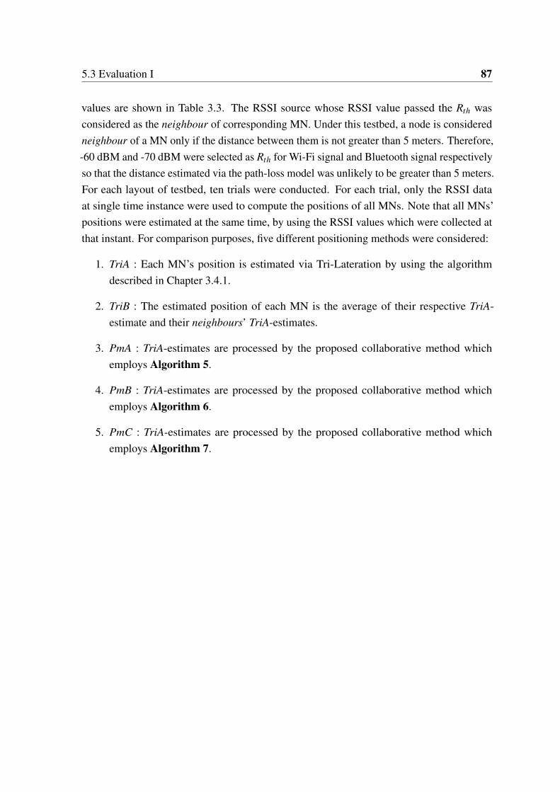
5.3 Evaluation I 87
values are shown in Table 3.3. The RSSI source whose RSSI value passed the Rth wasconsidered as the neighbour of corresponding MN. Under this testbed, a node is consideredneighbour of a MN only if the distance between them is not greater than 5 meters. Therefore,-60 dBM and -70 dBM were selected as Rth for Wi-Fi signal and Bluetooth signal respectivelyso that the distance estimated via the path-loss model was unlikely to be greater than 5 meters.For each layout of testbed, ten trials were conducted. For each trial, only the RSSI dataat single time instance were used to compute the positions of all MNs. Note that all MNs’positions were estimated at the same time, by using the RSSI values which were collected atthat instant. For comparison purposes, five different positioning methods were considered:
1. TriA : Each MN’s position is estimated via Tri-Lateration by using the algorithmdescribed in Chapter 3.4.1.
2. TriB : The estimated position of each MN is the average of their respective TriA-estimate and their neighbours’ TriA-estimates.
3. PmA : TriA-estimates are processed by the proposed collaborative method whichemploys Algorithm 5.
4. PmB : TriA-estimates are processed by the proposed collaborative method whichemploys Algorithm 6.
5. PmC : TriA-estimates are processed by the proposed collaborative method whichemploys Algorithm 7.

88 Collaborative Indoor Positioning based on Directed Graph
The errors of all ten trials for all five different methods in respective layouts of tesbed areshown in Figure 5.5. The error metric is the absolute difference between the MN’s estimatedposition and actual position. In Figure 5.5, each box-plot shows the distribution of NT ×Nm
errors where NT is the number of trials conducted and Nm is the number of MNs involved.It is worth mentioning that the mean of errors does not represent well the performance of apositioning method. Upper quartile, median and inter-quartile range should be the figures ofmerit instead. The lower the upper quartile or median, the higher the accuracy. The shorterthe inter-quartile range, the higher the consistency. Therefore, from Figure 5.5, it is apparentthat regardless of which layout, the five methods arranged in the order from lowest to highestpositioning performance are TriA, TriB, PmA, PmB and PmC. Though insignificant, PmAdoes outperform both PmB and PmC in layout no.4. More comparisons among PmA, PmBand PmC shall be discussed later.
Number of references vs. Number of neighbours vs. Errors
While correcting the estimated position of an MN, the proposed method basically considersany other nodes – which can be directly or indirectly linked to in the graph, as references.Note that the nodes which are directly linked to MN are neighbours, while the indirectlylinked ones are non-neighbours. The number of neighbours each MN has might vary at anytime t because it depends on whether the RSSI values given by surrounding nodes pass theRSSI thresholds. The number of references each i-th MN has is equivalent to the numberof j-th nodes which contribute non-zero and finite Si, j. Figure 5.6, Figure 5.7, Figure 5.8and Figure 5.9 summarize some information regarding the ten trials conducted in respectivelayouts. Each of these four Figures consists of three charts: firstly, the top chart shows thenumber of references made available from the graph for every trial, where the red horizontalline denotes the supposed number of available references; secondly, the middle chart illustratethe distribution of number of neighbours for every trial; thirdly, the bottom chart presents thedistribution of errors yielded from three different proposed methods in every trial. As for thetop charts, the fact that the number of references made available by the constructed graphfail to meet the supposed value in some trials implies that the Bluetooth RSSI data were notreliable enough to ensure that all MNs can detect their respective neighbours successfully.Nevertheless, by comparing the top charts with the middle charts, we can observe that thenumber of available references in most of the trials approach/reach the supposed value eventhough the number of neighbours a MN has may be as low as 1. Note that the number ofavailable references in trial no.8 for layout no.3 exceeds the maximum value by 1 because‘AP4’, owing to erratic Wi-Fi RSSI, was accidentally considered as neighbour of 8-th MN.By comparing the middle charts with the bottom charts, it seems that there is no correlation

5.3 Evaluation I 89
itioning Accuracy
TriA TriB PmA PmB PmC0
2
4
6
8
10
12
14
16
Method
Erro
r (m
)
Errors for Layout no.1
TriA TriB PmA PmB PmC0
2
4
6
8
10
12
14
Method
Erro
r (m
)
Errors for Layout no.2
TriA TriB PmA PmB PmC0
2
4
6
8
10
12
14
Method
Erro
r (m
)
Errors for Layout no.3
TriA TriB PmA PmB PmC0
2
4
6
8
10
12
14
Method
Erro
r (m
)
Errors for Layout no.4
Fig. 5.5 Errors of five different methods for four different layouts of testbed.
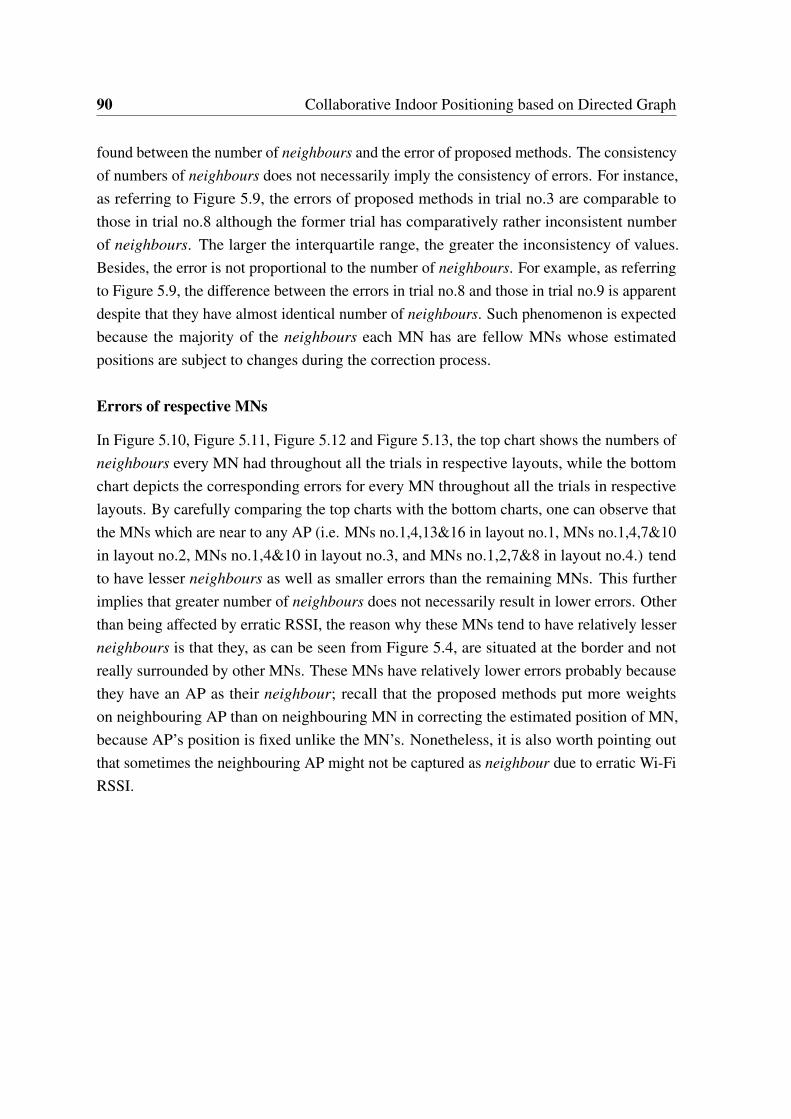
90 Collaborative Indoor Positioning based on Directed Graph
found between the number of neighbours and the error of proposed methods. The consistencyof numbers of neighbours does not necessarily imply the consistency of errors. For instance,as referring to Figure 5.9, the errors of proposed methods in trial no.3 are comparable tothose in trial no.8 although the former trial has comparatively rather inconsistent numberof neighbours. The larger the interquartile range, the greater the inconsistency of values.Besides, the error is not proportional to the number of neighbours. For example, as referringto Figure 5.9, the difference between the errors in trial no.8 and those in trial no.9 is apparentdespite that they have almost identical number of neighbours. Such phenomenon is expectedbecause the majority of the neighbours each MN has are fellow MNs whose estimatedpositions are subject to changes during the correction process.
Errors of respective MNs
In Figure 5.10, Figure 5.11, Figure 5.12 and Figure 5.13, the top chart shows the numbers ofneighbours every MN had throughout all the trials in respective layouts, while the bottomchart depicts the corresponding errors for every MN throughout all the trials in respectivelayouts. By carefully comparing the top charts with the bottom charts, one can observe thatthe MNs which are near to any AP (i.e. MNs no.1,4,13&16 in layout no.1, MNs no.1,4,7&10in layout no.2, MNs no.1,4&10 in layout no.3, and MNs no.1,2,7&8 in layout no.4.) tendto have lesser neighbours as well as smaller errors than the remaining MNs. This furtherimplies that greater number of neighbours does not necessarily result in lower errors. Otherthan being affected by erratic RSSI, the reason why these MNs tend to have relatively lesserneighbours is that they, as can be seen from Figure 5.4, are situated at the border and notreally surrounded by other MNs. These MNs have relatively lower errors probably becausethey have an AP as their neighbour; recall that the proposed methods put more weightson neighbouring AP than on neighbouring MN in correcting the estimated position of MN,because AP’s position is fixed unlike the MN’s. Nonetheless, it is also worth pointing outthat sometimes the neighbouring AP might not be captured as neighbour due to erratic Wi-FiRSSI.

5.3 Evaluation I 91
Layout 1
1 2 3 4 5 6 7 8 9 10
17
19
Trial no.
Am
ount
of r
efer
ence
s
4
6
8
10
12
14
1 2 3 4 5 6 7 8 9 10Trial no.
Am
ount
of n
eigh
bour
s
1 2 3 4 5 6 7 8 9 100
2
4
6
8
10
Trial no.
Erro
r (m
)
PmAPmBPmC
Fig. 5.6 Trials’ results for layout no.1.

92 Collaborative Indoor Positioning based on Directed Graph
Layout 2
1 2 3 4 5 6 7 8 9 10
15
17
19
Trial no.
Am
ount
of r
efer
ence
s
4
6
8
10
12
1 2 3 4 5 6 7 8 9 10Trial no.
Am
ount
of n
eigh
bour
s
1 2 3 4 5 6 7 8 9 100
2
4
6
8
10
12
Trial no.
Erro
r (m
)
PmAPmBPmC
Fig. 5.7 Trials’ results for layout no.2.

5.3 Evaluation I 93
Layout 3
1 2 3 4 5 6 7 8 9 10
9
11
13
Trial no.
Am
ount
of r
efer
ence
s
3
4
5
6
7
8
9
1 2 3 4 5 6 7 8 9 10Trial no.
Am
ount
of n
eigh
bour
s
1 2 3 4 5 6 7 8 9 100
2
4
6
8
10
Trial no.
Erro
r (m
)
PmAPmBPmC
Fig. 5.8 Trials’ results for layout no.3.

94 Collaborative Indoor Positioning based on Directed Graph
Layout 4
1 2 3 4 5 6 7 8 9 10
6
8
10
12
Trial no.
Am
ount
of r
efer
ence
s
1
2
3
4
5
6
1 2 3 4 5 6 7 8 9 10Trial no.
Am
ount
of n
eigh
bour
s
1 2 3 4 5 6 7 8 9 100
2
4
6
8
10
Trial no.
Erro
r (m
)
PmAPmBPmC
Fig. 5.9 Trials’ results for layout no.4.

5.3 Evaluation I 95La
yout
1 468101214
12
34
56
78
910
1112
1314
1516
MN
no.
Amount of neighbours
12
34
56
78
910
1112
1314
1516
01234567891011
MN
no.
Error (m)
P
mA
Pm
BP
mC
Fig.
5.10
Tria
ls’r
esul
tsfo
rlay
outn
o.1
(Re-
arra
nged
).

96 Collaborative Indoor Positioning based on Directed GraphLa
yout
2 4681012
12
34
56
78
910
1112
1314
1516
MN
no.
Amount of neighbours
12
34
56
78
910
1112
1314
1516
024681012
MN
no.
Error (m)
P
mA
Pm
BP
mC
Fig.
5.11
T ria
ls’r
esul
tsfo
rlay
outn
o.2
(Re-
arra
nged
).

5.3 Evaluation I 97La
yout
3
468
12
34
56
78
910
MN
no.
Amount of neighbours
12
34
56
78
910
01234567891011
MN
no.
Error (m)
P
mA
Pm
BP
mC
Fig.
5.12
Tria
ls’r
esul
tsfo
rlay
outn
o.3
(Re-
arra
nged
).

98 Collaborative Indoor Positioning based on Directed GraphLa
yout
4 246
12
34
56
78
MN
no.
Amount of neighbours
12
34
56
78
01234567891011
MN
no.
Error (m)
P
mA
Pm
BP
mC
Fig.
5.13
T ria
ls’r
esul
tsfo
rlay
outn
o.4
(Re-
arra
nged
).

5.3 Evaluation I 99
Impact of lesser references on Errors of proposed method
One novel feature of the proposed collaborative method is the usage of directed graph toacquire more references before applying the correction algorithm. The references primarilycomprise the neighbouring nodes, and possibly include the neighbouring nodes of neighbour-ing nodes as well as the distant ones. The proposed correction algorithm then makes useof every available references to refine the estimated position via iterating Multi-Laterationwith custom weighted averaging. PmA, PmB and PmC could also be modified in order thatonly the neighbours of respective MNs are used as references, by replacing the line no.3 ofAlgorithm 5, Algorithm 6 and Algorithm 7 with "if j-th node is a neighbour of i-th nodethen". From Figure 5.14 that compares the errors of original versions to those of modifiedversions, it is apparent that, except for PmA, the original versions outperform the modifiedversions in all four layouts. Therefore, one can deduce that greater number of referencesconsidered during correction is likely to mitigate the errors more effectively.
Impact of varying number of BNs on Errors of proposed method
As previously mentioned, BNs are more influential than MNs while refining the MN’s esti-mated position (Pi,z). To examine the impact of having BNs on the correction’s effectiveness,the number of Wi-Fi APs allowed to be included in the graph was varied according to casesshown in Table 5.1. Note that the APs were regarded as BNs, and the number of APs allowed
Table 5.1 Number of APs allowed to be included in the Directed Graph for different cases
Case APs allowed
1 AP1, AP2, AP3, AP42 AP1, AP2, AP33 AP1, AP24 AP15 None
does not always equate to the number of BNs existing in the graph because sometimes theAP may not be captured as neighbour to any MNs even though they are indeed very nearby.Figure 5.15 compares the errors of all three proposed methods in all five cases for all fourlayouts. Here, the accuracy metric is the upper quartile of the boxplot. The lower the upperquartile, the higher the accuracy. From Figure 5.15, one can observe that: firstly, the accuracyof all three proposed methods deteriorates as the number of APs allowed decreases; secondly,highest accuracy’s deterioration rate goes to PmA, followed by PmB and then PmC; thirdly,

100 Collaborative Indoor Positioning based on Directed Graph
PmA PmB PmC0
1
2
3
4
5
6
7
8
Method
Erro
r (m
)
Errors for Layout no.1
OriginalModified
PmA PmB PmC0
2
4
6
8
10
Method
Erro
r (m
)
Errors for Layout no.2
OriginalModified
PmA PmB PmC0
2
4
6
8
10
12
14
Method
Erro
r (m
)
Errors for Layout no.3
OriginalModified
PmA PmB PmC0
2
4
6
8
10
Method
Erro
r (m
)
Errors for Layout no.4
OriginalModified
Fig. 5.14 Errors of proposed methods: All references versus Neighbours only.

5.3 Evaluation I 101
among the three, PmC has the highest accuracy in all cases except case 5 for layout no.4.Figure 5.16 shows one of the trials’ results in case 5 where BN is absent from the graph. FromFigure 5.16, it is apparent that the positions estimated by PmC visually form a distributionthat considerably matches the MNs’ actual positions, yet the distribution is slightly turnedclockwise and swayed to the right. The distribution could be shifted westward if ‘AP4’were a neighbour of 4-th MN. This is because the estimated position of 4-th MN might beshifted towards ‘AP4’, thereby also somewhat "pulling" the estimated positions of other MNstowards the same directions. Generally, in whichever direction the distribution sways to, aBN needs to be available at opposite direction to mitigate the sway.
Discussion
By comparing the errors (upper quartiles) of PmA, PmB and PmC shown in Figure 5.15with the errors (upper quartiles) of TriB shown in Figure 5.5, one can observe that: firstly,PmA seemingly outperforms TriB only in cases 1 & 2 for all four layouts; secondly, TriBoutperforms PmB only in cases 4 & 5 for layout no.3 as well as in case 5 for layout no.4;thirdly, PmC outperforms TriB in all cases for any layouts except case 5 for layout no.4.Such statistics implies two things: firstly, PmA, PmB and PmC are deemed pointless in theaforementioned cases because TriB outperforms them despite being comparatively muchsimpler in terms of computation/algorithm; secondly, among the three proposed methods,PmC is the most robust towards the lack of BNs.
Admittedly, Beacon Node is not always available at the right place to anchor the MNs’estimated positions, and therefore alternative way of anchoring is necessary. One potentialway to mitigate the sway of distribution is shifting the whole distribution until its centroidmatches with the centroid of actual positions. An illustration for such shifting is depicted inFigure 5.17. Note that the estimated positions and actual positions in reality are unlikely tobe so neatly arranged. Figure 5.18, Figure 5.19, Figure 5.20 and Figure 5.21 depict the errorsof proposed methods before and after shifting. From these four Figures, it is apparent that, inany cases and layouts, the errors after the shifting reduce and also become more consistent.However, the main problem with such shifting is locating the actual centroid while the actualpositions of all MNs are originally unknown. Nevertheless, the actual centroid could bepossibly found if we know how the MNs are distributed within a known area, e.g. if thepeople (MNs) are somewhat evenly scattered within a hall, then the actual centroid is simplyassumed the centroid of the hall.

102 Collaborative Indoor Positioning based on Directed Graph
erent cases
PmA PmB PmC0
2
4
6
8
10
12
14
Method
Erro
r (m
)
Errors of Proposed Methods for Layout no.1.
Case 1Case 2Case 3Case 4Case 5
PmA PmB PmC0
2
4
6
8
10
12
14
Method
Erro
r (m
)
Errors of Proposed Methods for Layout no.2.
Case 1Case 2Case 3Case 4Case 5
PmA PmB PmC0
2
4
6
8
10
12
Method
Erro
r (m
)
Errors of Proposed Methods for Layout no.3.
Case 1Case 2Case 3Case 4Case 5
PmA PmB PmC0
2
4
6
8
10
12
14
Method
Erro
r (m
)
Errors of Proposed Methods for Layout no.4.
Case 1Case 2Case 3Case 4Case 5
Fig. 5.15 Errors in all five cases for all four layouts.
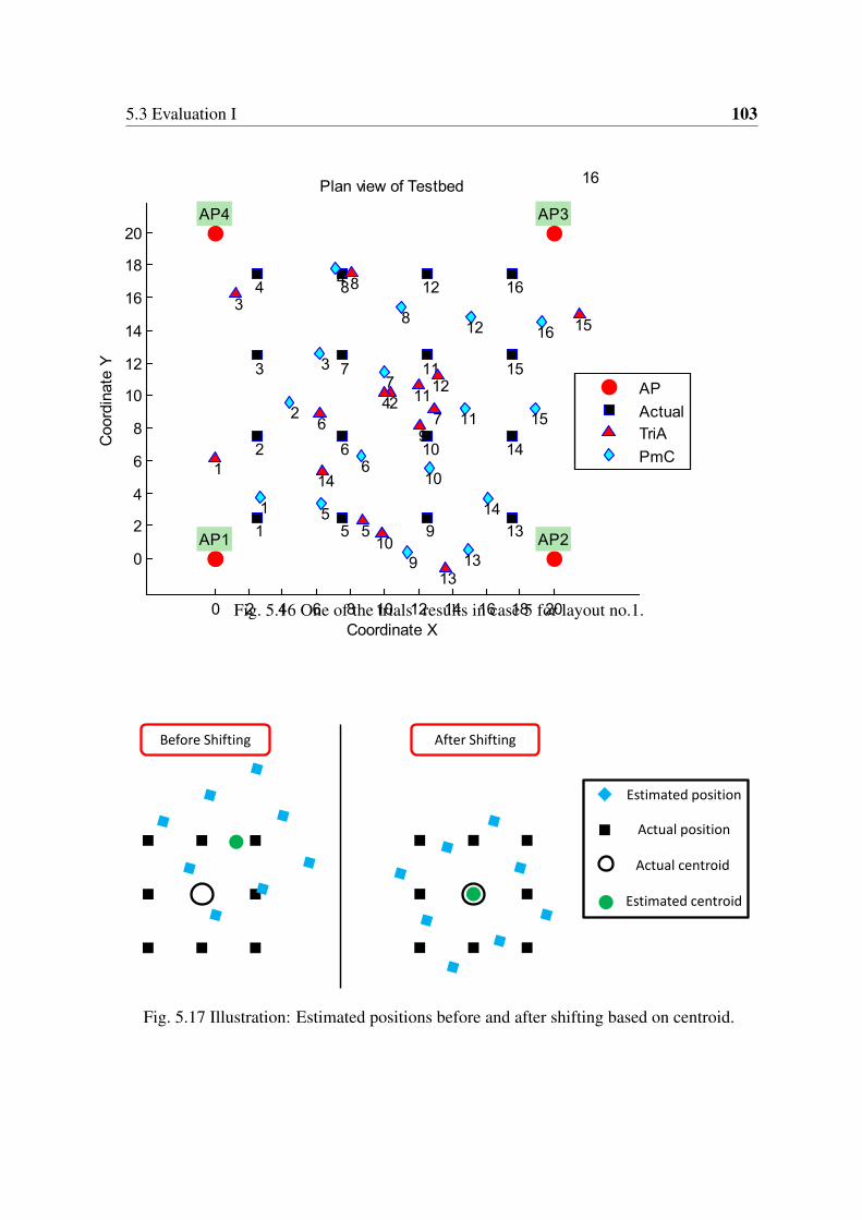
5.3 Evaluation I 103
0 2 4 6 8 10 12 14 16 18 20
0
2
4
6
8
10
12
14
16
18
20
Coordinate X
Coo
rdin
ate
Y
Plan view of Testbed
AP1 AP2
AP3AP4
1
2
3
4
5
6
7
8
9
10
11
12
13
14
15
16
1
2
3
4
5
6 7
8
9
10
1112
13
14
15
16
1
2
3
4
5
6
7
8
9
10
11
12
13
14
15
16
APActualTriAPmC
Fig. 5.16 One of the trials’ results in case 5 for layout no.1.
Before Shifting After Shifting
Estimated position
Actual position
Actual centroid
Estimated centroid
Fig. 5.17 Illustration: Estimated positions before and after shifting based on centroid.

104 Collaborative Indoor Positioning based on Directed Graph
1 2 3 4 50
5
10
15
Case
Erro
r (m
)Errors of PmA under different cases for Layout no.1.
BeforeAfter
1 2 3 4 50
2
4
6
8
Case
Erro
r (m
)
Errors of PmB under different cases for Layout no.1.
BeforeAfter
1 2 3 4 50
2
4
6
8
Case
Erro
r (m
)
Errors of PmC under different cases for Layout no.1.
BeforeAfter
Fig. 5.18 Errors of proposed methods Before and After shifting (Layout no.1).

5.3 Evaluation I 105
1 2 3 4 50
5
10
15
Case
Erro
r (m
)Errors of PmA under different cases for Layout no.2.
BeforeAfter
1 2 3 4 50
2
4
6
8
Case
Erro
r (m
)
Errors of PmB under different cases for Layout no.2.
BeforeAfter
1 2 3 4 50
2
4
6
8
Case
Erro
r (m
)
Errors of PmC under different cases for Layout no.2.
BeforeAfter
Fig. 5.19 Errors of proposed methods Before and After shifting (Layout no.2).

106 Collaborative Indoor Positioning based on Directed Graph
1 2 3 4 50
5
10
15
Case
Erro
r (m
)Errors of PmA under different cases for Layout no.3.
BeforeAfter
1 2 3 4 50
5
10
15
Case
Erro
r (m
)
Errors of PmB under different cases for Layout no.3.
BeforeAfter
1 2 3 4 50
5
10
15
Case
Erro
r (m
)
Errors of PmC under different cases for Layout no.3.
BeforeAfter
Fig. 5.20 Errors of proposed methods Before and After shifting (Layout no.3).

5.3 Evaluation I 107
1 2 3 4 50
5
10
15
Case
Erro
r (m
)Errors of PmA under different cases for Layout no.4.
BeforeAfter
1 2 3 4 50
5
10
15
Case
Erro
r (m
)
Errors of PmB under different cases for Layout no.4.
BeforeAfter
1 2 3 4 50
5
10
15
Case
Erro
r (m
)
Errors of PmC under different cases for Layout no.4.
BeforeAfter
Fig. 5.21 Errors of proposed methods Before and After shifting (Layout no.4).

108 Collaborative Indoor Positioning based on Directed Graph
5.4 Evaluation II
Figure 5.22 shows the plane view of the testbed used to evaluate the efficacy of proposedcollaborative method in improving the positions estimated by some PDR -based positioningmethods. Note that the four Wi-Fi APs at the site were just deployed to provide RSSI data,and they were not utilized as BNs by the proposed collaborative method under this testbed.
20 25 30 35 40 45 50 55 6018
23
28
33
38
1 2 3 4 5
6 7 8 9 10
1 2 3 4 5
6 7 8 9 10
Coordinate X
Coo
rdin
ate
Y
Plan view of Testbed
AP1 AP2
AP3AP4
Start positionsEnd positions
Fig. 5.22 Plane view of testbed.
A total of ten trials were conducted. In each trial, ten MNs walked a long straight path fromtheir respective start positions until the end positions, and their positions were estimated byfive different PDR based methods which are listed as follows:
1. PdrA: Sole PDR, as explained in Chapter 3.3.
2. PdrB: PDR with Markov Chain Monte Carlo sampling, explained in Chapter 3.4.3.
3. PdrC: PDR with Sampling Importance Resampling, explained in Chapter 3.4.2.
4. PdrD: PDR with heading correction, as explained in Chapter 4.2.

5.4 Evaluation II 109
The initial headings of all MNs were provided. However, all MNs were required to makefew random turnings at their start positions before commencing the walk, and the resultantheadings were estimated by using Equation (3.4). The random turnings before the walk wereintended to introduce some heading errors in order to simulate unreliable PDR. Note thatPDR is well known for being vulnerable to erroneous heading. Then, when all MNs reachedtheir respective end positions, the proposed collaborative method was executed to correct theend positions estimated by the aforementioned PDR based methods.
Besides, another collaborative method was also applied to correct the position estimatesgiven by aforementioned PDR based methods, and the corresponding results were comparedwith those of proposed collaborative method. This method, which is adapted from [81],corrects the estimated position of each MN via a Kalman Filter based algorithm summarizedby Algorithm 8. In Algorithm 8, t denotes the time instance, Pt−1 is MN’s estimatedposition provided by PdrA, PdrB, PdrC or PdrD; both A and H are 2×2 identity matrices;Q and R are the measurement noise covariance and process noise covariance respectively,which are 2× 2 identity matrices multiplied with some appropriate scalars; and the errorcovariance P is initially zero.
Algorithm 8 Collaborative method adapted from [81]1: Predict next state: x← A×Pt−1
2: Predict next covariance: Pt ← A×Pt−1×A⊺+Q3: Compute Kalman gain: K← Pt×H⊺ (H×Pt×H⊺+R)4: if This MN has any neighbours then5: Obtain measurement: zt ← average of estimated positions of all neighbours6: Update predicted state: x← x+K× (zt−H× x)7: Update predicted covariance: Pt ← Pt−K×H×Pt
8: end if9: Finalize estimated position: Pt ← x
The error metric is the absolute difference between MN’s actual end position and es-timated end position. Figure 5.23 compares the errors of all aforementioned PDR basedmethods before and after being refined by the collaborative method, and each boxplot showthe distribution of NT ×Nm errors where Nt is the number of trials and Nm is the numberof MNs. Note that PM denotes the proposed collaborative method while EM denotes thecollaborative method described by Algorithm 8.
From Figure 5.23, it is apparent that PM outperforms EM in correcting the estimatedend positions of PdrA, PdrB and PdrD respectively. Besides, the errors of both PdrA and

110 Collaborative Indoor Positioning based on Directed Graph
PdrA PdrB PdrC PdrD0
2
4
6
8
10
12
14
16
18
Method
Erro
r (m
)
BeforeAfter PMAfter EM
PdrA PdrB PdrC PdrD0
2
4
6
8
10
12
Method
Erro
r (m
)
BeforeAfter PMAfter EM
Fig. 5.23 Errors of four different PDR based methods: Before and After correction bycollaborative method.
PdrC before correction are similar, yet differ considerably after correction; the reason behindthis can be comprehended by referring to a trial’s results shown in Figure 5.24. FromFigure 5.24, one can observe that: firstly, the PM-corrected estimates are not as spread out asthe non-corrected estimates, in other words, the separation distances among the estimatesare somewhat improved after correction; secondly, the centroid of non-corrected estimatessomewhat determines the centroid of corrected estimates; thirdly, PM-corrected estimatesof both PdrA and PdrD, as compared to those of PdrB and PdrC, are distributed relativelycloser to the actual positions. This therefore deduces that the correction by PM is likely tobe more effective when the centroid of non-corrected estimates is nearer to the centroid ofactual positions, though the separation distances among non-corrected estimates might beoverly large.
Basically, PM corrects the estimated positions by adjusting the separation distancesamong them, and the resultant estimates do not necessarily become closer to their respectiveactual positions. For example, referring to the PdrB-estimates shown in Figure 5.23, thecorrection causes the estimated position of MN no.10 to shift further apart from its actualposition, while significantly improves its separation distances from estimated positions ofmultiple MNs (i.e. MN no.1, MN no.4, MN no.5, MN no.6, MN no.7, and MN no.8).

5.4 Evaluation II 111
1820
2224
2628
3032
3436
242628303234363840
12
34
56
78
910
12
3
4
5
678
9
10
12
34
5
678
9
10
12
3
4
5
678
9
10
Coo
rdin
ate
X
Coordinate Y
End
pos
ition
s es
timat
ed b
y P
drA
Act
ual
Bef
ore
Afte
r PM
Afte
r EM
2025
3035
242526272829303132
12
34
5
67
89
10
1
2
34
56
7
8
9
10
1
2
34
56
78
9
10
1
2
34
56
7
8
9
10
Coo
rdin
ate
X
Coordinate Y
End
pos
ition
s es
timat
ed b
y P
drB
Act
ual
Bef
ore
Afte
r PM
Afte
r EM
2224
2628
3032
34252627282930313233
12
34
5
67
89
101
2 3
4
5
6
7
8
9
10
1
2
34
56
7
89
10
12 34
56
7
8
9
10
Coo
rdin
ate
X
Coordinate Y
End
pos
ition
s es
timat
ed b
y P
drC
A
ctua
lB
efor
eA
fter P
MA
fter E
M
1820
2224
2628
3032
34252627282930313233
12
34
5
67
89
10
1
2
34
56 7
89
10
12
34
56
78
9
10
12
34
5
6 78
9
10
Coo
rdin
ate
X
Coordinate Y
End
pos
ition
s es
timat
ed b
y P
drD
Act
ual
Bef
ore
Afte
r PM
Afte
r EM
Fig.
5.24
End
posi
tions
estim
ated
byfo
urdi
ffer
entP
DR
base
dm
etho
ds(i
nfir
sttr
ial)
.

112 Collaborative Indoor Positioning based on Directed Graph
2025
3035
4045
5055
6023283338
Coo
rdin
ate
X
Coordinate Y
Traj
ecto
ries
estim
ated
by
Pdr
A 12
34
56
78
910
12
34
56
78
910
2025
3035
4045
5055
6023283338
Coo
rdin
ate
X
Coordinate Y
Traj
ecto
ries
estim
ated
by
Pdr
C 12
34
56
78
910
12
34
56
78
910
2025
3035
4045
5055
6023283338
Coo
rdin
ate
X
Coordinate Y
Traj
ecto
ries
estim
ated
by
Pdr
B 12
34
56
78
910
12
34
56
78
910
2025
3035
4045
5055
6023283338
Coo
rdin
ate
XCoordinate Y
Traj
ecto
ries
estim
ated
by
Pdr
D 12
34
56
78
910
12
34
56
78
910
Fig.
5.25
Traj
ecto
ries
estim
ated
byfo
urdi
ffer
entP
DR
base
dm
etho
ds(i
nfir
sttr
ial)
.

5.5 Summary 113
5.5 Summary
This chapter proposes a collaborative positioning method that is based on Directed Graph.The positions of all MNs can be initially estimated via either PDR or RSSI-based Tri-Lateration. The directed graph is used to express the relations among the nodes (both MNsand BNs). From the graph, the shortest distances from each MN to all other nodes may bederived. The derived shortest distances, are then utilized to correct the estimated position ofeach MN via an iterative process. In every iteration of correction process, estimated positionof each MN is finalized by averaging the sample points. The sample points are generatedbased on the derived shortest distances via a Particle Filter. Among the sample points, onlythose which are resulted from neighbouring BNs hold comparatively greater weights. Theproposed collaborative positioning method had been tested via simulation. The test results arepresented to demonstrate the feasibility and efficacy of the proposed method. The accuracyof proposed method is likely to improve when BNs are available at the right spots to mitigatethe skewness of finalized estimates.


Chapter 6
Conclusion
6.1 Summary
In view of arising demand for indoor location based services (LBS), many indoor positioningsystems (IPS) have been developed by leveraging various technologies such as Micro-Electro-Mechanical Systems (MEMS), Radio Frequency Identification (RFID). However, none ofthese existing IPS are gaining mainstream adoption as much as their outdoor counterparti.e. GPS, probably owing to their corresponding implementation cost. The implementationcost of an IPS includes the resources required for system’s start-up and maintenance, aswell as constraints that might be imposed to the users. Perhaps the most promising IPS arethose which leverage the smart-devices (i.e. smartphones and tablets), because smart-devicesare increasingly widespread and they are richly equipped with capabilities like GPS, Wi-Fi, Bluetooth and motion detection. With such capabilities of smart-device, various sortsof positioning algorithms are made possible and their underlying techniques are typicallyPedestrian Dead-Reckoning (PDR), Lateration and Fingerprinting.
PDR estimates the pedestrian’s present position by advancing their last known positionwith heading and distance which are derived from data of motion sensors, i.e. accelerome-ters, gyroscopes and magnetometers. PDR is well known for its relatively high positioningaccuracy which deteriorates over time due to inherent sensors’ biases and drifts. Unlike PDRwhich can be implemented on smart-device alone, Lateration and Fingerprinting requirenecessary devices to be deployed at the site to enable wireless transmission between de-vices. Lateration deduces the pedestrian’s position based on RSSI-derived distance betweenpedestrian and reference device, while Fingeprinting infers pedestrian’s position by matchingonline RSSI measurements with pre-collected RSSI measurements. Albeit the latter, as com-pared to the former, is more reliable and robust towards erratic RSSI data, its implementation

116 Conclusion
is comparatively more complex. Further discussion regarding the fundamentals of indoorpositioning and related work are presented in Chapter 2.
In Chapter 4, two schemes that improve PDR’s long-term positioning accuracy byutilizing the RSSI of Wi-Fi signals are proposed. The implementation of either schemeis deemed low-cost since Wi-Fi APs are prevalent especially among the indoors. Upondetecting strong RSSI value, the first scheme ensures that the estimated position lies withinacceptable region around the corresponding Wi-Fi AP. Subsequently, the estimated positioncan be further refined if the bearing of the pedestrian from that AP is known. The secondscheme, on the other hand, corrects the PDR-estimated headings based on linear regression,and subsequently updates the PDR-estimated positions. However, it is triggered only upondetecting a long straight PDR-estimated trajectory. Nevertheless, such trajectory is commonlyobserved in pedestrian’s daily movements such as walking down the long corridors withinthe university or mega-mall. Both schemes had been proven feasible at real sites within theSwinburne University of Technology Sarawak Campus, and experimental results show thatPDR with proposed schemes outperform some existing PDR -based positioning methods interms of accuracy and robustness.
More information taken into consideration is likely to result in more reliable estimation,and thus positioning methods that estimate individual pedestrian’s position by utilizingsurrounding pedestrians’ information are gaining interest among IPS researchers. Suchcollaborative methods are promising due to the fact that the pedestrians usually cluster eitherknowingly or unknowingly among themselves, and most of them carry pervasive-computingdevices such as smart-devices and laptops. Therefore, in Chapter 5, a novel collaborativepositioning method that makes use of directed graph is proposed. The directed graph isconstructed to express the relations among the pedestrians and site’s anchors/APs. Thepedestrians’ positions are initially estimated via either PDR or RSSI-based Tri-Lateration,and then refined by a Particle Filter based algorithm according to the information derivedfrom the graph. Both experimental and simulation results suggest the feasibility and efficacyof the proposed method.

6.2 Future Research Work 117
6.2 Future Research Work
There are several issues that can be explored to further refine the methods proposed in thisthesis, and a number of them are listed as follows:
1. As mentioned in Chapter 4.2.1, all elements of series, regardless of whether they areoutliers, are indiscriminately considered in deriving the linear regression line. Theimpact of outliers on the orientation of linear regression line should be investigated asin which and how many outliers among the series’ elements can be useful or negligible.Subsequently, weighted linear regression may also be attempted.
2. During the heading correction, the original headings (estimated by PDR) are simplyreplaced by the headings which are derived based on linear regression. Admittedly, thederived headings are not always more accurate than the original headings. Perhaps apotential way to achieve more reliable heading correction is by combining the originalheadings with the derived headings via some kinds of filters. Alternatively, indoorfloor plan (if provided) may be useful in determining whether heading correction isnecessary – for example, if the original long straight trajectory does not cross anyboundaries, then heading correction is not needed. Furthermore, the re-estimatedtrajectory (which is resulted from corrected headings) should also reasonably alignwith the floor plan [44, 57, 61].
3. As mentioned in Chapter 5.2, the neighbouring BNs are considered more reliablereferences than other nodes while adjusting the estimated position of individual pedes-trian. However, BNs (i.e. Wi-Fi APs) might not be in near vicinity of pedestrianclusters at all times, and therefore alternative source of reliable references is needed. Insuch cases, pedestrians may be considered as reliable references if they fulfill certaincriteria - for example, being stationary for a period of time and moving in the samegroups. In addition, the weight of each reference may be assigned according to thecriteria it fulfills.
4. As described in Chapter 5.4, the proposed collaborative method was executed onlywhen all MNs reached their respective actual end positions. In other words, only thePDR-estimated end positions experience the correction. It was intended under thepresumption that, by the time the MN arrives at the end of route, the position errorwould reach a stage where correction is necessary. At short intervals, the PDR accuracyis relatively high, and so the correction may seem unnecessary. Therefore, the righttiming for the correction should be investigated.

118 Conclusion
5. For the proposed collaborative method to work effectively, all MNs are required tomonitor RSSI from surrounding nodes continuously. Such requirement may causethe proposed collaborative method prohibitively complex and energy heavy besidescompromising on privacy issues. This, however, is not discussed in this work becausethe proposed collaborative method was designed so merely as an effort to examine thepossibility of achieving reliable indoor positioning by making use of the collaborationamong pervasive computing devices.
6. The proposed schemes are heavily reliant on empirically defined parameters andthresholds which are likely to differ across different device models. Different devicesmay observe dissimilar RSSI values even at same position. Moreover, they may varyin terms of scan response time, sensor readings, etc.

References
[1] Abadi, M. J., Luceri, L., Hassan, M., Chou, C. T., and Nicoli, M. (2014). A collaborativeapproach to heading estimation for smartphone-based pdr indoor localisation. In IndoorPositioning and Indoor Navigation (IPIN), 2014 International Conference on, pages554–563.
[2] Abdulrahim, K., Moore, T., Hide, C., and Hill, C. (2014). Understanding the performanceof zero velocity updates in mems-based pedestrian navigation. International Journal ofAdvancements in Technology, 5(2):53–60.
[3] Ahmed, S. H., Bouk, S. H., Javaid, N., and Sasase, I. (2012). Combined human, antennaorientation in elevation direction and ground effect on rssi in wireless sensor networks. InFrontiers of Information Technology (FIT), 2012 10th International Conference on, pages46–49.
[4] Alarifi, A., Al-Salman, A., Alsaleh, M., Alnafessah, A., Al-Hadhrami, S., Al-Ammar,M. A., and Al-Khalifa, H. S. (2016). Ultra wideband indoor positioning technologies:Analysis and recent advances. Sensors, 16(5).
[5] Arulampalam, M., Maskell, S., Gordon, N., and Clapp, T. (2002). A tutorial on particlefilters for online nonlinear/non-gaussian bayesian tracking. Signal Processing, IEEETransactions on, 50(2):174–188.
[6] AT&T Laboratories Cambridge (2005 [cited 19 August 2016]). The bat ultrasoniclocation system. Available from: http://www.cl.cam.ac.uk/research/dtg/attarchive/bat/.
[7] Au, A. W. S., Feng, C., Valaee, S., Reyes, S., Sorour, S., Markowitz, S. N., Gold, D.,Gordon, K., and Eizenman, M. (2013). Indoor tracking and navigation using receivedsignal strength and compressive sensing on a mobile device. IEEE Transactions on MobileComputing, 12(10):2050–2062.
[8] Bertram, J. and Ruina, A. (2001). Multiple walking speed-frequency relations arepredicted by constrained optimization. Journal of Theoretical Biology, 209:445–453.
[9] Bolic, M., Rostamian, M., and Djuric, P. M. (2015). Proximity detection with rfid: Astep toward the internet of things. IEEE Pervasive Computing, 14(2):70–76.
[10] Carrillo, D., Moreno, V., Úbeda, B., and Skarmeta, A. F. (2015). Magicfinger: 3dmagnetic fingerprints for indoor location. Sensors, 15(7).

120 References
[11] Chan, L.-w., Chiang, J.-r., Chen, Y.-c., Ke, C.-n., Hsu, J., and Chu, H.-h. (2006). Col-laborative localization: Enhancing wifi-based position estimation with neighborhood linksin clusters. In Proceedings of the 4th International Conference on Pervasive Computing,PERVASIVE’06, pages 50–66, Berlin, Heidelberg. Springer-Verlag.
[12] Chen, Z. (2003). Bayesian filtering: From Kalman Filters to Particle Filters, andBeyond.
[13] Cho, S. Y. and Park, C. G. (2006). Mems based pedestrian navigation system. Journalof Navigation, 59:135–153.
[14] Constandache, I., Choudhury, R. R., and Rhee, I. (2010). Towards mobile phonelocalization without war-driving. In INFOCOM, 2010 Proceedings IEEE, pages 1–9.
[15] Correa, A., Barcelo, M., Morell, A., and Lopez Vicario, J. (2014). Enhanced inertial-aided indoor tracking system for wireless sensor networks: A review. Sensors Journal,IEEE, 14(9):2921–2929.
[16] Dardari, D., Closas, P., and Djuric, P. (2015). Indoor tracking: Theory, methods, andtechnologies. Vehicular Technology, IEEE Transactions on, 64(4):1263–1278.
[17] Dias, M. H. C. and Siqueira, G. L. (2005). Indoor tdoa-aoa measurements at the 3gsystems frequency band – a simple approach. Journal of Communication and InformationSystems, 20(3):112–124.
[18] Fang, L., Antsaklis, P., Montestruque, L., McMickell, M., Lemmon, M., Sun, Y., Fang,H., Koutroulis, I., Haenggi, M., Xie, M., and Xie, X. (2005). Design of a wirelessassisted pedestrian dead reckoning system - the navmote experience. IEEE Transactionson Instrumentation and Measurement, 54(6):2342–2358.
[19] Foxlin, E. (2005). Pedestrian tracking with shoe-mounted inertial sensors. IEEEComputer Graphics and Applications, 25(6):38–46.
[20] Graefenstein, J., Albert, A., Biber, P., and Schilling, A. (2009). Wireless node localiza-tion based on rssi using a rotating antenna on a mobile robot. In Positioning, Navigationand Communication, 2009. WPNC 2009. 6th Workshop on, pages 253–259.
[21] Graefenstein, J. and Bouzouraa, M. E. (2008). Robust method for outdoor localizationof a mobile robot using received signal strength in low power wireless networks. InRobotics and Automation, 2008. ICRA 2008. IEEE International Conference on, pages33–38.
[22] Gu, Y., Lo, A., and Niemegeers, I. (2009). A survey of indoor positioning systems forwireless personal networks. IEEE Communications Surveys Tutorials, 11(1):13–32.
[23] Gusenbauer, D., Isert, C., and Krösche, J. (2010). Self-contained indoor positioning onoff-the-shelf mobile devices. In Indoor Positioning and Indoor Navigation (IPIN), 2010International Conference on, pages 1–9.
[24] Harle, R. (2013). A survey of indoor inertial positioning systems for pedestrians. IEEECommunications Surveys Tutorials, 15(3):1281–1293.

References 121
[25] He, S. and Chan, S. H. G. (2016). Wi-fi fingerprint-based indoor positioning: Recentadvances and comparisons. IEEE Communications Surveys Tutorials, 18(1):466–490.
[26] He, Y. and Bilgic, A. (2011). Iterative least squares method for global positioningsystem. Advances in Radio Science, 9:203–208.
[27] Hightower, J. and Borriello, G. (2001). Location systems for ubiquitous computing.Computer, 34(8):57–66.
[28] Higuchi, T., Fujii, S., Yamaguchi, H., and Higashino, T. (2014). Mobile node local-ization focusing on stop-and-go behavior of indoor pedestrians. IEEE Transactions onMobile Computing, 13(7):1564–1578.
[29] Higuchi, T., Yamaguchi, H., and Higashino, T. (2012). Clearing a crowd: Context-supported neighbor positioning for people-centric navigation. In Proceedings of the 10thInternational Conference on Pervasive Computing, Pervasive’12, pages 325–342, Berlin,Heidelberg. Springer-Verlag.
[30] Honkavirta, V., Perala, T., Ali-Loytty, S., and Piche, R. (2009). A comparative surveyof wlan location fingerprinting methods. In Positioning, Navigation and Communication,2009. WPNC 2009. 6th Workshop on, pages 243–251.
[31] Iwase, T. and Shibasaki, R. (2013). Infra-free indoor positioning using only smartphonesensors. In International Conference on Indoor Positioning and Indoor Navigation (IPIN),pages 1–8.
[32] J. Kim, H. Jang, D. H. and Park, C. (2004). A step, stride and heading determination forthe pedestrian navigation system. Journal of Global Positioning Systems, 3(1-2):273–279.
[33] Jimenez, A., Seco, F., Prieto, C., and Guevara, J. (2009). A comparison of pedestriandead-reckoning algorithms using a low-cost mems imu. In IEEE International Symposiumon Intelligent Signal Processing. WISP 2009., pages 37–42.
[34] Jin, Y., Motani, M., Soh, W. S., and Zhang, J. (2010). Sparsetrack: Enhancing indoorpedestrian tracking with sparse infrastructure support. In INFOCOM, 2010 ProceedingsIEEE, pages 1–9.
[35] Jin, Y., Soh, W.-S., Motani, M., and Wong, W.-C. (2013). A robust indoor pedestriantracking system with sparse infrastructure support. Mobile Computing, IEEE Transactionson, 12(7):1392–1403.
[36] Jin, Y., Toh, H.-S., Soh, W.-S., and Wong, W.-C. (2011). A robust dead-reckoningpedestrian tracking system with low cost sensors. In IEEE International Conference onPervasive Computing and Communications (PerCom), pages 222–230.
[37] Jo, C. and Lee, C. (2016). Multilateration method based on the variance of estimateddistance in range-free localisation. Electronics Letters, 52(12):1078–1080.
[38] Kalman, D. (2002). An underdetermined linear system for gps. The College Mathemat-ics Journal, 33:384–390.

122 References
[39] Khmou, Y., Safi, S., and Frikel, M. (2014). Comparative Study between SeveralDirection of Arrival Estimation Methods. Journal of Telecommunications and InformationTechnology, 1:41–48.
[40] Klingbeil, L. and Wark, T. (2008). A wireless sensor network for real-time indoorlocalisation and motion monitoring. In Information Processing in Sensor Networks, 2008.IPSN ’08. International Conference on, pages 39–50.
[41] Lan, K.-C. and Shih, W.-Y. (2014). Using smart-phones and floor plans for indoorlocation tracking. IEEE Transactions on Human-Machine Systems, 44(2):211–221.
[42] Lee, B. G. and Chung, W. Y. (2011). Multitarget three-dimensional indoor navigationon a pda in a wireless sensor network. IEEE Sensors Journal, 11(3):799–807.
[43] Levi, R. and Judd, T. (1996). Dead reckoning navigational system using accelerometerto measure foot impacts. US Patent 5,583,776.
[44] Li, F., Zhao, C., Ding, G., Gong, J., Liu, C., and Zhao, F. (2012). A reliable and accurateindoor localization method using phone inertial sensors. In Proceedings of the 2012 ACMConference on Ubiquitous Computing, UbiComp ’12, pages 421–430, New York, NY,USA. ACM.
[45] Liew, L. S. and Wong, W. S. H. (2016). Improved pedestrian dead-reckoning-basedindoor positioning by rssi-based heading correction. IEEE Sensors Journal, 16(21):7762–7773.
[46] Lingwen Zhang, C. T. and Yang, G. (2011). Wireless positioning: Fundamentals,systems and state of the art signal processing techniques. Cellular Networks - Positioning,Performance Analysis, Reliability.
[47] Liu, H., Darabi, H., Banerjee, P., and Liu, J. (2007). Survey of wireless indoorpositioning techniques and systems. IEEE Transactions on Systems, Man, and Cybernetics,Part C: Applications and Reviews, 37(6):1067–1080.
[48] Liu, H. F., Ren, W., Zhang, T., Gong, J., m. Liang, J., Liu, B., w. Shi, J., and Huang,Z. (2014). An adaptive selection algorithm of threshold value in zero velocity updatingfor personal navigation system. In Control Conference (CCC), 2014 33rd Chinese, pages1035–1038.
[49] Liu, Y., Wang, Q., Liu, J., and Wark, T. (2012). Mcmc-based indoor localization with asmart phone and sparse wifi access points. In IEEE International Conference on PervasiveComputing and Communications Workshops (PERCOM Workshops), pages 247–252.
[50] Luo, M. (2013). Indoor radio propagation modeling for system performance prediction.PhD dissertation, INSA de Lyon.
[51] Luo, Y., Hoeber, O., and Chen, Y. (2013). Enhancing wi-fi fingerprinting for indoorpositioning using human-centric collaborative feedback. Human-centric Computing andInformation Sciences, 3(1):1–23.

References 123
[52] Mahfouz, S., Mourad-Chehade, F., Honeine, P., Farah, J., and Snoussi, H. (2016).Non-parametric and semi-parametric rssi/distance modeling for target tracking in wirelesssensor networks. IEEE Sensors Journal, 16(7):2115–2126.
[53] Mardeni, R. and Nizam, O. S. (2010). Node positioning in zigbee network usingtrilateration method based on the received signal strength indicator (rssi). EuropeanJournal of Scientific Research, 46(1):48–61.
[54] Müller, P., Raitoharju, M., Ali-Löytty, S., Wirola, L., and Piché, R. (2016). A survey ofparametric fingerprint-positioning methods. Gyroscopy and Navigation, 7(2):107–127.
[55] Nikitin, P. V., Martinez, R., Ramamurthy, S., Leland, H., Spiess, G., and Rao, K. V. S.(2010). Phase based spatial identification of uhf rfid tags. In 2010 IEEE InternationalConference on RFID (IEEE RFID 2010), pages 102–109.
[56] Noh, Y., Yamaguchi, H., Lee, U., Vij, P., Joy, J., and Gerla, M. (2013). Clips:Infrastructure-free collaborative indoor positioning scheme for time-critical team opera-tions. In Pervasive Computing and Communications (PerCom), 2013 IEEE InternationalConference on, pages 172–178.
[57] Pai, D., Malpani, M., Sasi, I., Aggarwal, N., and Mantripragada, P. (2012). Padati: Arobust pedestrian dead reckoning system on smartphones. In IEEE 11th InternationalConference on Trust, Security and Privacy in Computing and Communications (TrustCom),pages 2000–2007.
[58] Payal, A., Rai, C. S., and Reddy, B. V. R. (2015). Experimental analysis of some radiopropagation models for smart wireless sensor networks applications. In SAI IntelligentSystems Conference (IntelliSys), 2015, pages 338–342.
[59] Pierlot, V. and Droogenbroeck, M. V. (2014). A new three object triangulation algorithmfor mobile robot positioning. IEEE Transactions on Robotics, 30(3):566–577.
[60] Rafael Berkvens, Dries Vandermeulen, C. V. H. P. and Weyn, M. (2014). Feasibility ofgeomagnetic localization and geomagnetic ratslam. International Journal on Advances inSystems and Measurements, 7(1&2):44–56.
[61] Rai, A., Chintalapudi, K. K., Padmanabhan, V. N., and Sen, R. (2012). Zee: Zero-effortcrowdsourcing for indoor localization. In Proceedings of the 18th Annual InternationalConference on Mobile Computing and Networking, Mobicom ’12, pages 293–304, NewYork, NY, USA. ACM.
[62] Rice, A. and Harle, R. (2005). Evaluating lateration-based positioning algorithms forfine-grained tracking. In Proceedings of the 2005 Joint Workshop on Foundations ofMobile Computing, DIALM-POMC ’05, pages 54–61, New York, NY, USA. ACM.
[63] Ruizhi, C., Ling, P., and Yuwei, C. (2011). A smart phone based pdr solution for indoornavigation. In Proceedings of the 24th International Technical Meeting of the SatelliteDivision of the Institute of Navigation (ION GNSS 2911), pages 1404–1408.
[64] S. H. Shin, C. G. Park, H. S. H. and Lee, J. M. (2005). Mems-based personal navigatorequipped on the user’s body. In Proceedings of the 18th International Technical Meeting ofthe Satellite Division of The Institute of Navigation (ION GNSS 2005), pages 1998–2002.

124 References
[65] Sarkar, T. K., Ji, Z., Kim, K., Medouri, A., and Salazar-Palma, M. (2003). A survey ofvarious propagation models for mobile communication. IEEE Antennas and PropagationMagazine, 45(3):51–82.
[66] Schiller, J. and Voisard, A. (2004). Location Based Services. Morgan KaufmannPublishers Inc., San Francisco, CA, USA.
[67] Shabbir, N., Sadiq, M. T., Kashif, H., and Ullah, R. (2011). Comparison of radiopropagation models for long term evolution (LTE) network. CoRR, abs/1110.1519.
[68] Shao, H. J., Zhang, X. P., and Wang, Z. (2014). Efficient closed-form algorithms foraoa based self-localization of sensor nodes using auxiliary variables. IEEE Transactionson Signal Processing, 62(10):2580–2594.
[69] Simon, D. (2010). Kalman filtering with state constraints: a survey of linear andnonlinear algorithms. IET Control Theory Applications, 4(8):1303–1318.
[70] Smith, A. and Breen, T. (2007). Use of geo-stationary satellites to augment wide_areamultilateration synchronization. US Patent App. 11/343,079.
[71] Steinhoff, U. and Schiele, B. (2010). Dead reckoning from the pocket - an experimentalstudy. In IEEE International Conference on Pervasive Computing and Communications(PerCom), pages 162–170.
[72] Stromback, P., Rantakokko, J., Wirkander, S.-L., Alexandersson, M., Fors, K., Skog, I.,and Handel, P. (2010). Foot-mounted inertial navigation and cooperative sensor fusion forindoor positioning. In Proceedings of the 2010 International Technical Meeting of TheInstitute of Navigation, pages 89–98.
[73] Susi, M., Renaudin, V., and Lachapelle, G. (2013). Motion mode recognition and stepdetection algorithms for mobile phone users. Sensors, 13(2):1539.
[74] Taniuchi, D., Liu, X., Nakai, D., and Maekawa, T. (2015). Spring model basedcollaborative indoor position estimation with neighbor mobile devices. Selected Topics inSignal Processing, IEEE Journal of, 9(2):268–277.
[75] Wadhwa, M., Song, M., Rali, V., and Shetty, S. (2009). The impact of antennaorientation on wireless sensor network performance. In Computer Science and InformationTechnology, 2009. ICCSIT 2009. 2nd IEEE International Conference on, pages 143–147.
[76] Wang, B., Zhou, S., Liu, W., and Mo, Y. (2015). Indoor localization based on curvefitting and location search using received signal strength. IEEE Transactions on IndustrialElectronics, 62(1):572–582.
[77] Wang, H., Sen, S., Elgohary, A., Farid, M., Youssef, M., and Choudhury, R. R. (2012).No need to war-drive: Unsupervised indoor localization. In Proceedings of the 10thInternational Conference on Mobile Systems, Applications, and Services, MobiSys ’12,pages 197–210, New York, NY, USA. ACM.
[78] Want, R., Hopper, A., Falcão, V., and Gibbons, J. (1992). The active badge locationsystem. ACM Trans. Inf. Syst., 10(1):91–102.

References 125
[79] Weinberg, H. (2002). Using the adxl202 in pedometer and personal navigation applica-tions. Analog Devices AN-602 Application Note.
[80] Yang, C. and r. Shao, H. (2015). Wifi-based indoor positioning. IEEE CommunicationsMagazine, 53(3):150–157.
[81] Yang, Z., Feng, X., and Zhang, Q. (2014). Adometer: Push the limit of pedestrianindoor localization through cooperation. Mobile Computing, IEEE Transactions on,13(11):2473–2483.
[82] Zahid Farid, R. N. and Ismail, M. (2013). Recent advances in wireless indoor local-ization techniques and system. Journal of Computer Networks and Communications,2013.
[83] Zhang, R., Hoflinger, F., and Reindl, L. (2013). Inertial sensor based indoor localizationand monitoring system for emergency responders. Sensors Journal, IEEE, 13(2):838–848.
[84] Zhongliang, D., Yanpei, Y., Xie, Y., Neng, W., and Lei, Y. (2013). Situation anddevelopment tendency of indoor positioning. Communications, China, 10(3):42–55.
[85] Zhou, S. and Pollard, J. K. (2006). Position measurement using bluetooth. IEEETransactions on Consumer Electronics, 52(2):555–558.
