1

Accurate, fully-automated NMR spectral profilingfor metabolomics

Siamak Ravanbakhsh1,2, Philip Liu1,3, Trent C. Bjorndahl1,3, Rupasri Mandal1,3, Jason R. Grant1, Michael Wilson1,Roman Eisner1, Igor Sinelnikov3, Xiaoyu Hu4, Claudio Luchinat5, Russell Greiner1,2, and David S. Wishart1,3,6

1Department of Computing Science, University of Alberta, Edmonton, AB, Canada2Alberta Innovates Center for Machine Learning (AICML)

3Department of Biological Sciences, University of Alberta, Edmonton, AB, Canada4Fiorgen Foundation, 50019 Sesto Fiorentino, Italy

5Centro Risonanze Magnetiche (CERM/CIRMMP), University of Florence, 50019 Sesto Fiorentino, Italy6National Research Council, National Institute for Nanotechnology (NINT)

Abstract—Many diseases cause significant changes to the con-centrations of small molecules (a.k.a. metabolites) that appear in aperson’s biofluids, which means such diseases can often be readilydetected from a persons metabolic profile.This information canbe extracted from a person’s biofluids using NMR spectroscopy.Today, this is often done manually by trained experts, whichmeans this process is relatively slow, expensive and can be error-prone. A system that can quickly, accurately and autonomouslyproduce a person’s metabolic profile would enable efficient andreliable prediction of many such diseases from a single sample,which could significantly improve the way medicine is practiced.

This paper presents such a system: Given a 1D 1H NMRspectrum of a complex biofluid such as serum or CSF, ourBAYESIL system can automatically determine this metabolicprofile, and do so without any human guidance. This requiresfirst performing all of the required spectral processing steps(i.e., Fourier transformation, phasing, solvent-removal, chemicalshift referencing, baseline correction, lineshape convolution) thenmatching this resulting spectrum against a reference compoundlibrary, which contains the signatures of each relevant metabolite.Many of these processing steps are novel algorithms, and ourmatching step views spectral matching as an inference problemwithin a probabilistic graphical model that rapidly approximatesthe most probable metabolic profile.

Our extensive studies on a diverse set of complex mixtures(real biological samples, defined mixtures and realistic computergenerated spectra; each involving ∼ 50 compounds), show thatBAYESIL can autonomously and accurately find NMR-detectablemetabolites at concentrations as low as 2µM, in terms of bothidentification (∼ 90% correct) and quantification (∼ 10% error),in under 5 minutes on a single CPU processor. These resultsdemonstrate that BAYESIL is the first fully-automatic publicly-accessible system that provides quantitative NMR spectral pro-filing effectively – with an accuracy that meets or exceeds theperformance of highly trained human experts. We anticipate thistool will usher in high-throughput metabolomics and enable awealth of new applications of NMR in clinical settings. Userscan access BAYESIL at http://www.bayesil.ca.

Index Terms— NMR — Metabolomics — Targeted Profiling— Probabilistic Graphical Models NMR — Metabolomics —Targeted Profiling — Probabilistic Graphical Models—

Metabolomics is a relatively new branch of “omics” sciencethat focuses on the system-wide characterization of metabo-lites [1]. Metabolomics is often viewed as complementary to theother “omics” fields as it provides information about both an or-ganism’s phenotype and its environment. Because metabolomics

provides a unique window on gene-environment interactions, itis playing an increasingly important role in many quantitativephenotyping and functional genomics studies [2], [3], [4]. It is alsofinding more applications in disease diagnosis, biomarker discov-ery and drug development/discovery (e.g., [5], [6], [7]). This rapidgrowth in interest and excitement surrounding metabolomicsis also revealing its “Achilles heel”: Unlike proteomics, ge-nomics or transcriptomics, which are high-throughput sciences,metabolomics is a relatively low-throughput science. Compared togenomics, where it is now possible to automatically characterize1000s of genes, 100s of thousands of transcripts and millions ofSNPs in mere minutes, metabolomics only allows users to identifyand measure a few dozen metabolites after many hours of manualeffort. In other words, metabolomics is not automated. This prob-lem may stem from the history of metabolomics, as its analyticaltechniques, such as NMR spectroscopy, gas-chromatography-mass spectrometry (GC-MS) and liquid chromatography-massspectrometry (LC-MS), were originally developed for identifyingand quantifying pure compounds, not complex mixtures. Becausemost biological samples contain hundreds of metabolites, theresulting NMR, HPLC or LC-MS spectra usually contain hundredsor even thousands of peaks. The challenge in metabolomics,therefore, is to identify the mixture of compounds that producedthis forest of peaks. This compound identification process, calledspectral profiling, involves fitting the mixture spectrum to aset of individual pure reference spectra obtained from knowncompounds [8], [9]. If done correctly, the fitting process yields notonly the identity of the compounds, but also the concentrationof those compounds. Therefore, the end result of a successfulspectral profiling study is a table of metabolite names and theirabsolute or relative concentrations. Because spectral profilingis such a complex pattern recognition problem, it is often bestdone by a trained expert. However, this reliance on manual dataanalysis by a human expert is problematic, as it is slow andleads to inconsistent results, operator errors and reduced levelsof reproducibility [10].

The automation bottleneck in metabolomics is widely recog-nized, and has led to a number of efforts to accelerate or automatecompound identification and/or quantification in LC-MS, in GC-MS and in NMR spectroscopy. Some of the most active efforts in(semi)automated compound identification and quantification havebeen in NMR-based metabolomics. In particular, several softwarepackages have been developed that support semi-automatic NMRspectral profiling of 1D and 2D 1H NMR spectra, including somecommercial packages (e.g., [12], [14], [13]). There are tremen-dous differences in the quantification/identification capabilities,spectral database size, speed and instrument compatibility ofthese software tools. Furthermore, these packages either requiremanual fitting or manual spectral processing, or a bit of both;

arX

iv:1

409.

1456

v3 [

cs.A

I] 8

Sep

201

4

2

3.63.73.83.94.04.1

PPM

reconstruction

spectrum

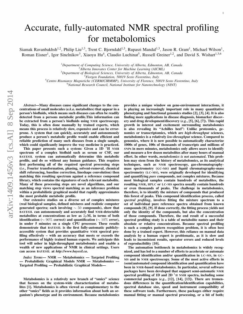
Fig. 1. This figure shows the crowded region (3.5-4.1 PPM) of a computer generated spectrum with 150 compounds (solid black) and the fit produced byBAYESIL (dashed red) as well as individual clusters as quantified by BAYESIL. Each cluster is free to shift a specified amount, which is at least 0.025 PPM.

see Appendix I for a comprehensive list of NMR softwares andtheir limitations. The need for such manual interventions leadsto a number of issues, including slower throughput, operatorfatigue and associated operator errors, the need for highly trainedand dedicated experts, the requirement of two or more spectralassessments for quality assessment and control purposes, andinconsistent results between individuals, between labs or overdifferent time periods [8], [10].

It would be better to have a software system that canautomatically perform both spectral processing and spectraldeconvolution, be able to analyze complex mixtures (∼60 com-pounds) quickly and accurately, and be able to produce reliablecompound concentrations. Here we describe such a system, calledBAYESIL.

Extensive testing, on computer-generated and laboratory-generated chemical mixtures as well as real biological samples,shows that BAYESIL consistently performs with ∼ 90% accuracyfor compound identification in mixtures with up to 60 differentmetabolites. It also determines metabolite concentrations with∼ 10% error. For computer-generated biofluid spectra, where theground truth is known, BAYESIL consistently outperforms highlytrained experts in both identification and quantification. BAYESILappears to be the first system that supports fully automated andfully quantitative NMR-based metabolomics. This paper describesthis system, its underlying algorithms and its performance acrossvarious tests.

I. METABOLIC PROFILING PIPELINE

BAYESIL performs fully automated spectral processing andspectral profiling for 1D 1H NMR spectra collected on eitherAgilent/Varian or Bruker instruments, at several different fre-quencies. In particular, it uses a variety of intelligent phasingand baseline correction methods to automatically process raw 1DNMR spectra (i.e., FIDs). It also uses approximate inference tech-niques to rapidly perform very accurate spectral deconvolution,yielding both compound identities and their concentrations. Herewe briefly describe BAYESIL’s spectral processing algorithms, theprinciples and rationale behind BAYESIL’s spectral deconvolutionmethod and the construction of BAYESIL’s spectral library.

A. Spectral Processing in BAYESIL

Successful NMR spectral profiling depends critically on thequality and uniformity of the starting NMR spectrum. Unfortu-nately, most spectral processing functions (i.e., phasing, baselinecorrection, solvent filtering, chemical shift referencing) are left

to the user. Given the complexity and large number of variables,values and filters that can be used, many view spectral processingmore as an art, rather than a science. Different perspectivesor different personal thresholds on what is a “good looking”NMR spectrum can potentially lead to very different resultsregarding what compounds are identified or which compoundsare accurately quantified in a biofluid spectrum. To addressthis issue, BAYESIL itself performs all of the spectral processingfunctions: starting from the FID, it performs zero-filling, Fourierand Hilbert transformation, phasing, baseline correction, chem-ical shift referencing, reference deconvolution and smoothing.Automating this process ensures reproducibility, consistency anduniformity of the input data prior to spectral deconvolution. Herewe briefly sketch some of the more challenging steps in thisprocess.

Phasing involves maximizing the symmetry of the peaks byreducing zero-order and first-order phase mismatch. Zero-orderphase mismatch is a sign of the difference between the referencephase and the receiver phase and is independent of frequency.The first-order phase mismatch can be a result of the time-delaybetween excitation and detection, flip-angle variation and thefilter that is used to reduce the noise outside of the spectralbandwidth [15]. In addition to using well-known techniques,such as spectral norm minimization [16], BAYESIL uses thecross entropy optimization method [11] to jointly maximize adirect measure of peak symmetry for isolated peaks across thespectrum.

Baseline correction involves removing distortions that mayarise from hardware artifacts or highly concentrated compo-nents of the mixture (e.g., solvent), while keeping the desirablesignal intact. This process is often performed in two steps: 1)baseline-detection and 2) modelling. BAYESIL relies on iterativethresholding [17] and estimating the signal-to-noise ratio to detectthe baseline points. It uses monotonic cubic Hermite interpolation[18] and Whittaker smoothing technique for baseline modelling[19].

BAYESIL also provides the options for smoothing and line-broadening using Savitzky-Golay [20] and Gaussian filters. How-ever smoothing is mostly cosmetic and it is not essential forspectral deconvolution. In fact, it may degrade the signal andoccasionally remove the the low-amplitude and narrow peaks.Similarly, we found the effect of reference deconvolution – whichmay be used to remove instrumental or experimentally induceddistortions of the Lorentzian lineshape – is also mostly cosmetic,and if the distortion around the reference peak has any sourceother than poor shimming, using reference deconvolution willhave an adverse effect on the rest of the NMR spectrum.

3

B. Spectral DeconvolutionAn NMR spectrum for a compound M is a collection of one

or more Lorentzian peaks formed into one or more clusters –that is, each compound M is a set of clusters {Ck}, where eachcluster Ck is set of peaks, and each peak is defined by a triple,θ = (θ1, θ2, θ3) corresponding to its height, center and width (athalf height) respectively – where the height at x due to this peakis q(x;θ) = θ1θ3

θ3+4(θ2−x)2. Letting X refer to the entire spectrum

(e.g., from -1 to 13 PPM when referenced against the DSS peak),the height of the spectrum of a pure compoundM at each locationx ∈ X , is

s(x ;M, ρM, δM) = ρM∑C∈M

∑θ∈C

q(x− δC ;θ) (1)

where ρM is the concentration of this compound and δM ={δC | C ∈ M} is the set of chemical shifts for the clusters associatedwith this compound.

An NMR spectrum is essentially a linear combination of thepeaks in its component compounds: that is, the height at eachPPM value x of a mixture spectrum is just the sum of the contribu-tions of each compound. This means, given the concentrations ofthe compounds ρ = {ρM}, and the chemical shifts δ =

⋃M δM

of the clusters associated with these compounds, we can then“draw” an NMR spectrum – i.e., the height at each PPM x, giventhis ρ and δ, is s(x ;ρ, δ) =

∑M s(x ;M, ρM, δM).

The spectral deconvolution challenge, in general, is the reverseprocess: Given a set of compounds {M1, . . . ,Mr} with associatedsignatures (i.e., θ values of their peaks, organized in clusters)and the observed spectrum s(·), find the “best” combination ofconcentrations ρ and shifts δ to fit that spectrum. To determinewhich values are best, for now, we consider a simple lossfunction that is the (square of the) difference of the heightsbetween the observed spectrum s(·) and the reconstructedspectrum s(· ; δ,ρ)

`X ( s(·), s(· ;ρ, δ) ) =

∫x∈X

(s(x)− s(x ;ρ, δ)

)2dx (2)

where the subscript X indicates that this loss function applies tothe entire spectrum; see Appendix II for BAYESIL’s actual lossfunction.

Our task is to find the values of

[ρ∗, δ∗] = argρ,δ min `X (s(·), s(· ;ρ, δ)) (3)

that minimize this loss function. Figure 1 shows part of a spec-trum over a complex mixture, and BAYESIL’s solution obtainedby minimizing the loss function.

This corresponds to search over a huge space – all possibleshifts for each of the clusters, and all possible concentrationsover the compounds. The key innovation of BAYESIL is howit minimizes this highly non-linear loss function, efficiently. Inparticular, BAYESIL “factors” this large task into a set of inter-related smaller tasks. Two characteristics of the NMR spectramake this factorization possible: 1) each shift is over only a smallrange (typically a window of ±0.025 PPM); and 2) as the height inthe spectrum due to a Lorentzian peak diminishes quadraticallyfrom its center, each peak and therefore each cluster can only“influence” a small interval; see Appendix III.

Now consider a function that maps each point in the spectrumto the set of clusters that might affect the height at this location.That is, given the set of compounds {M} that might appear in aparticular biofluid (e.g., the 48 that can appear in CSF), we canidentify each PPM location x ∈ X with the small set of clustersthat might influence it, C(x).

We can then partition the spectrum into disjoint contiguousregions, {XI}, where every PPM location in each XI involvesexactly the same subset of clusters – i.e., for any pair of pointsx1, x2 ∈ XI , we know that C(x1) = C(x2). For example, ourlibrary for CSF includes 48 compounds, with a total of 180clusters and 946 peaks. A typical CSF spectrum is partitioned into

0.60.70.80.91.01.11.21.3

PPM

DSS(1)DSS(2)DSS(3)DSS(4)1-Methylhistidine(1)

1-Methylhistidine(2)

1-Methylhistidine(3)1-Methylhistidine(4)1-Methylhistidine(5)1-Methylhistidine(6) 2-Hydroxybutyrate(1)

2-Hydroxybutyrate(2)

2-Hydroxybutyrate(3)

2-Hydroxybutyrate(4)

Acetic acid(1)Betaine(1)

Betaine(2)

Acetoacetate(1)Acetoacetate(2) L-Carnitine(1)

L-Carnitine(2)

L-Carnitine(3)

L-Carnitine(4)

L-Carnitine(5)

L-Carnitine(6)

Creatine(1)

Creatine(2)

Citric acid(1)

Citric acid(2)

Citric acid(3)

Choline(1)Choline(2)

Choline(3) Ethanol(1)

Ethanol(2)

D-Glucose(1)

D-Glucose(2)

D-Glucose(3)

D-Glucose(4)

D-Glucose(5)

D-Glucose(6)

D-Glucose(7)

D-Glucose(8)

D-Glucose(9)

D-Glucose(10)

D-Glucose(11)

D-Glucose(12)

D-Glucose(13)

D-Glucose(14) Glycine(1)

Glycerol(1)

Glycerol(2)

Glycerol(3)

Formic acid(1) L-Glutamic acid(1)

L-Glutamic acid(2)

L-Glutamic acid(3)

L-Glutamic acid(4)

Hypoxanthine(1)

Hypoxanthine(2)

L-Tyrosine(1)

L-Tyrosine(2)

L-Tyrosine(3)

L-Tyrosine(4)

L-Tyrosine(5)

L-Phenylalanine(1)

L-Phenylalanine(2)

L-Phenylalanine(3)

L-Phenylalanine(4)

L-Phenylalanine(5)

L-Phenylalanine(6) L-Alanine(1)

L-Alanine(2)

L-Proline(1)

L-Proline(2)

L-Proline(3)

L-Proline(4)

L-Proline(5)

L-Threonine(1)

L-Threonine(2)

L-Threonine(3)

L-Asparagine(1)

L-Asparagine(2)

L-Asparagine(3)

L-Asparagine(4)

L-Isoleucine(1)

L-Isoleucine(2)

L-Isoleucine(3)L-Isoleucine(4)L-Isoleucine(5)

L-Isoleucine(6)

L-Histidine(1)

L-Histidine(2)

L-Histidine(3)

L-Histidine(4)

L-Histidine(5)

Lysine(1)

Lysine(2)Lysine(3)

Lysine(4)

Lysine(5)

L-Serine(1)

L-Serine(2)

L-Serine(3)

L-Lactic acid(1)

L-Lactic acid(2)

L-Aspartic acid(1)

L-Aspartic acid(2)

L-Aspartic acid(3)

L-Cystine(1)

L-Cystine(2)L-Cystine(3)

Ornithine(1)

Ornithine(2)

Ornithine(3)

Ornithine(4)

Ornithine(5)

Pyruvic acid(1)

Succinic acid(1)

Urea(1)

3-Hydroxybutyric acid(1)

3-Hydroxybutyric acid(2)

3-Hydroxybutyric acid(3)

3-Hydroxybutyric acid(4)

L-Arginine(1)

L-Arginine(2)

L-Arginine(3)

L-Arginine(4)

L-Arginine(5)

Creatinine(1)

Creatinine(2)

L-Cysteine(1)

L-Cysteine(2)

L-Cysteine(3)

L-Glutamine(1)

L-Glutamine(2)

L-Glutamine(3)

L-Glutamine(4)

L-Glutamine(5)

L-Leucine(1)

L-Leucine(2)

L-Leucine(3)

Malonic acid(1)

L-Methionine(1)

L-Methionine(2)L-Methionine(3)

L-Methionine(4)

Isopropanol(1)

Isopropanol(2)

L-Valine(1)

L-Valine(2)

L-Valine(3)

L-Valine(4)

L-Tryptophan(1)

L-Tryptophan(2)

L-Tryptophan(3)

L-Tryptophan(4)L-Tryptophan(5)

L-Tryptophan(6)

L-Tryptophan(7)

L-Tryptophan(8)

Acetone(1)

Methanol(1)

Propylene glycol(1)

Propylene glycol(2)

Propylene glycol(3)

Propylene glycol(4)

Dimethylsulfone(1)

Isobutyric acid(1)

Isobutyric acid(2)

reconstruction

spectrum

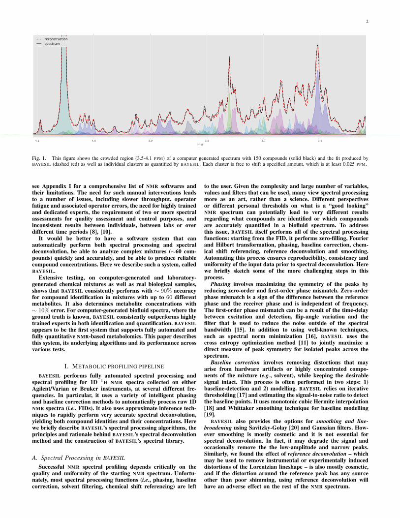
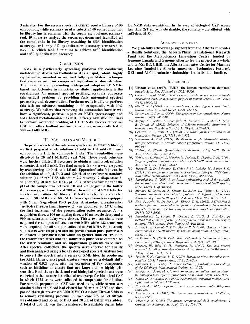
Fig. 2. Partitioning of X into continuous blocks XI ⊂ X for a part of ahuman serum spectrum. Here each block is shown with a different shade ofblue, below the horizontal axis. The domain of influence of each cluster isalso indicated with coloured blocks.

∼350 regions. Each of these regions will involve between 1 and∼25 clusters, and span between 0.0001 and 1.5 PPM. Moreover,each cluster will appear in between 1 and ∼70 different regions.

Figure 2 shows the division of a part of human serum NMRspectrum into regions XI ; blocks in different shades of blue.For example the region X[.8563,9289] from 0.8563 to 0.9289 PPMmight include significant contributions from the first cluster of 2-Hydroxybutyrate, the first cluster of L-Isoleucine and/or the firstcluster of L-Leucine. The region immediately to its left (from0.9289 to 0.9370 PPM) includes these and also a cluster of L-Valine, and the one to the right (from 0.8563 to 0.87526 PPM)does not include L-Isoleucine.

As the loss function `(·, ·) is additive over the domain X , wecan rewrite the optimization of eq[3] as the sum of the losses foreach of the regions XI :

[ρ∗, δ∗] = argρ,δ min∑I

`XI

(s(·), s(· ;ρI , δI)

)(4)

Now recall that each region XI involves relatively few compoundsand clusters. This suggests a preliminary step of simply “solving”each region, by itself: i.e., find the best centers for the clustersin that region δI , and the best concentrations for the associatedcompounds ρI , which collectively minimize the loss over the PPM-interval XI . This simple approach is fast, as it involves relativelyfew variables and a limited range of PPM-values. Unfortunately,this does not produce the overall correct answer – that is, eachregion has an opinion about the concentration and shift valuesof its cluster, and when two (or more) regions each involve thesame variable, they must both agree on its value.

To address this problem, we take a probabilistic approach,viewing the task of minimizing the loss function eq[2] as findingthe “Maximum a Posteriori” (MAP) assignment – i.e., the assign-ment to all of the cluster-shift and compound-concentration [δ,ρ]variables that makes the observed data as likely as possible. Here,the Boltzmann formula gives the probabilistic interpretation ofthe loss (a.k.a. the energy)

P(ρ, δ | s(·) ) = 1

Zexp

{− 1

T`X(s(·), s(· ;ρ, δ)

)}(5)

where Z is the normalization constant and T is known as the“temperature” parameter, explained in Appendix IV. Using thedecomposition of loss over regions (eq[4]) we can write thisdistribution in factored form

P(ρ, δ | s(·) ) = 1

Z

∏I

fI(ρI , δI)

fI(ρI , δI) = exp

{− 1

T`XI

(s(·), s(.;ρI , δI)

) }(6)

4

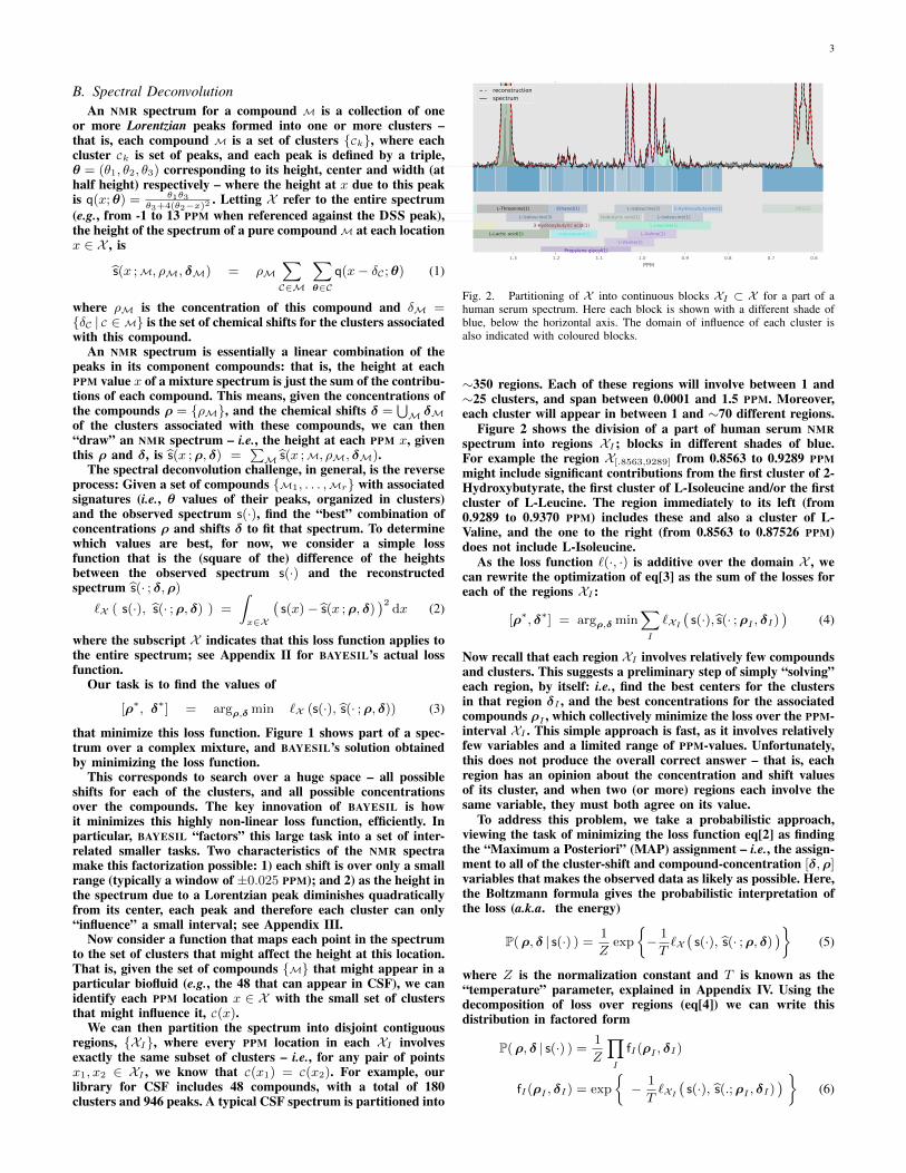
Fig. 3. Factor-graph for a library of 15 compounds immediately belowan associated NMR spectrum. Each factor is represented by a square andeach variable using a circle. Concentration (larger circles) and shift variables(smaller circles, beside the associated concentration) corresponding to eachcompound appear together. The position of each factor fI position in the plotcorresponds to the center of the corresponding block XI .

3.743.753.763.773.78

PPM

reconstruction

spectrum

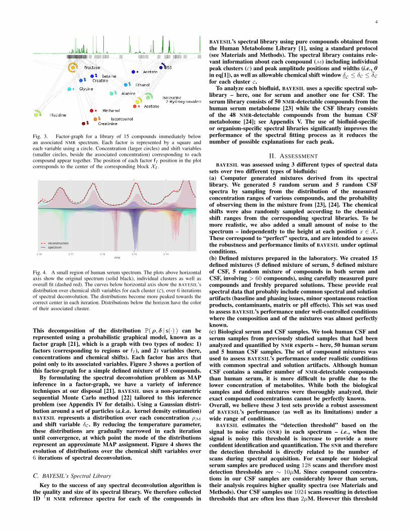
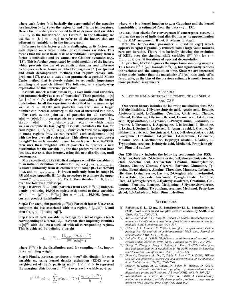
Fig. 4. A small region of human serum spectrum. The plots above horizontalaxis show the original spectrum (solid black), individual clusters as well asoverall fit (dashed red). The curves below horizontal axis show the BAYESIL’sdistribution over chemical shift variables for each cluster (C), over 6 iterationsof spectral deconvolution. The distributions become more peaked towards thecorrect center in each iteration. Distributions below the horizon have the colorof their associated cluster.

This decomposition of the distribution P(ρ, δ | s(·) ) can berepresented using a probabilistic graphical model, known as afactor graph [21], which is a graph with two types of nodes: 1)factors (corresponding to regions or fI ), and 2) variables (here,concentrations and chemical shifts). Each factor has arcs thatpoint only to its associated variables. Figure 3 shows a portion ofthis factor-graph for a simple defined mixture of 15 compounds.

By formulating the spectral deconvolution problem as MAPinference in a factor-graph, we have a variety of inferencetechniques at our disposal [21]. BAYESIL uses a non-parametricsequential Monte Carlo method [22] tailored to this inferenceproblem (see Appendix IV for details). Using a Gaussian distri-bution around a set of particles (a.k.a. kernel density estimation)BAYESIL represents a distribution over each concentration ρMand shift variable δC . By reducing the temperature parameter,these distributions are gradually narrowed in each iterationuntil convergence, at which point the mode of the distributionsrepresent an approximate MAP assignment. Figure 4 shows theevolution of distributions over the chemical shift variables over6 iterations of spectral deconvolution.

C. BAYESIL’s Spectral Library

Key to the success of any spectral deconvolution algorithm isthe quality and size of its spectral library. We therefore collected1D 1H NMR reference spectra for each of the compounds in

BAYESIL’s spectral library using pure compounds obtained fromthe Human Metabolome Library [1], using a standard protocol(see Materials and Methods). The spectral library contains rele-vant information about each compound (M) including individualpeak clusters (C) and peak amplitude positions and widths (i.e., θin eq[1]), as well as allowable chemical shift window δC ≤ δC ≤ δCfor each cluster C.

To analyze each biofluid, BAYESIL uses a specific spectral sub-library – here, one for serum and another one for CSF. Theserum library consists of 50 NMR-detectable compounds from thehuman serum metabolome [23] while the CSF library consistsof the 48 NMR-detectable compounds from the human CSFmetabolome [24]; see Appendix V. The use of biofluid-specificor organism-specific spectral libraries significantly improves theperformance of the spectral fitting process as it reduces thenumber of possible explanations for each peak.

II. ASSESSMENT

BAYESIL was assessed using 3 different types of spectral datasets over two different types of biofluids:(a) Computer generated mixtures derived from its spectrallibrary. We generated 5 random serum and 5 random CSFspectra by sampling from the distribution of the measuredconcentration ranges of various compounds, and the probabilityof observing them in the mixture from [23], [24]. The chemicalshifts were also randomly sampled according to the chemicalshift ranges from the corresponding spectral libraries. To bemore realistic, we also added a small amount of noise to thespectrum – independently to the height at each position x ∈ X .These correspond to “perfect” spectra, and are intended to assessthe robustness and performance limits of BAYESIL under optimalconditions.(b) Defined mixtures prepared in the laboratory. We created 15defined mixtures (5 defined mixture of serum, 5 defined mixtureof CSF, 5 random mixture of compounds in both serum andCSF, involving > 60 compounds), using carefully measured purecompounds and freshly prepared solutions. These provide realspectral data that probably include common spectral and solutionartifacts (baseline and phasing issues, minor spontaneous reactionproducts, contaminants, matrix or pH effects). This set was usedto assess BAYESIL’s performance under well-controlled conditionswhere the composition and of the mixtures was almost perfectlyknown.(c) Biological serum and CSF samples. We took human CSF andserum samples from previously studied samples that had beenanalyzed and quantified by NMR experts – here, 50 human serumand 5 human CSF samples. The set of compound mixtures wasused to assess BAYESIL’s performance under realistic conditionswith common spectral and solution artifacts. Although humanCSF contains a smaller number of NMR-detectable compoundsthan human serum, it is more difficult to profile due to thelower concentration of metabolites. While both the biologicalsamples and defined mixtures were thoroughly analyzed, theirexact compound concentrations cannot be perfectly known.Overall, we believe these 3 test sets provide a robust assessmentof BAYESIL’s performance (as well as its limitations) under awide range of conditions.

BAYESIL estimates the “detection threshold” based on thesignal to noise ratio (SNR) in each spectrum – i.e., when thesignal is noisy this threshold is increase to provide a moreconfident identification and quantification. The SNR and thereforethe detection threshold is directly related to the number ofscans during spectral acquisition. For example our biologicalserum samples are produced using 128 scans and therefore mostdetection thresholds are ∼ 10µM. Since compound concentra-tions in our CSF samples are considerably lower than serum,their analysis requires higher quality spectra (see Materials andMethods). Our CSF samples use 1024 scans resulting in detectionthresholds that are often less than 2µM. However this threshold

5

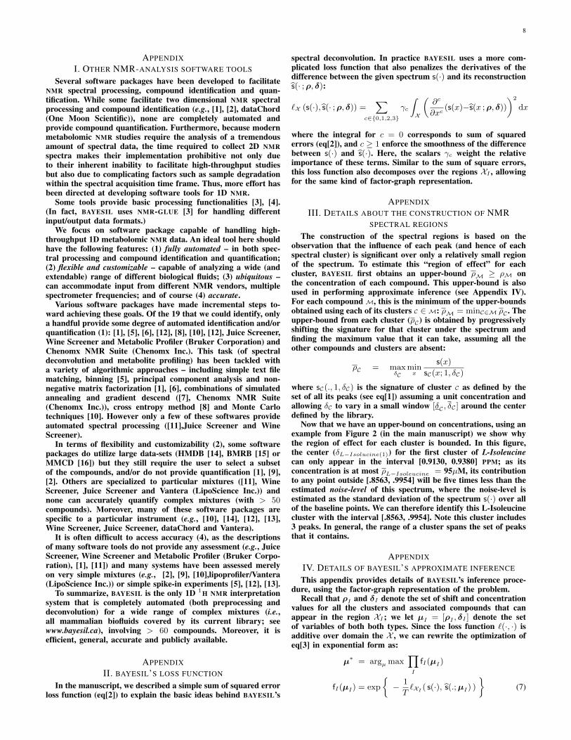
TABLE IIDENTIFICATION AND QUANTIFICATION ACCURACY OF BAYESIL AND HUMAN EXPERT ON VARIOUS DATA-SETS.

serum CSF complexbiological def. mix. comp. gen. biological def. mix. comp. gen. def. mix.

BAYESILid. accuracy .93± .04 .94± .02 .98± .01 .90± .04 .89± .03 .95± .03 .90± .02quant. accuracy .89± .02 .90± .02 .98± .01 .91± .01 .90± .02 .94± .02 .88± .02

expert id. accuracy - - .91± .02 - - .87± .05 -quant. accuracy - - .95± .01 - - .91± .04 -

AcetoacetateMalonic acid

L−TryptophanL−Asparagine

DimethylsulfoneIsobutyric acidHypoxanthine

Propylene glycolL−Aspartic acid

IsopropanolFormic acid

Ethanol2−Hydroxybutyrate

L−MethionineAcetone

Pyruvate/SuccinateBetaine

CreatineL−Histidine

1−MethylhistidineL−Carnitine

Choline3−Hydroxybutyric acid

DSSAcetic acidCitric acid

D−GlucoseGlycine

GlycerolL−Glutamic acid

L−TyrosineL−Phenylalanine

L−AlanineL−Proline

L−ThreonineL−Isoleucine

LysineL−Serine

L−Lactic acidL−ArginineCreatinine

L−GlutamineL−Leucine

L−ValineMethanol

0% 25% 50% 75% 100%Identification

True PositiveTrue NegativeFalse PositiveFalse Negative

101 102 103

Quantification (µM)

Avg. ThresholdAvg. ConcentrationAvg. Error

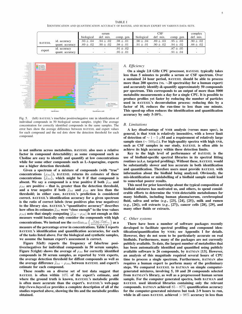
Fig. 5. (left) BAYESIL’s true/false positive/negative rate in identification ofindividual compounds in 50 biological serum samples. (right) The averageconcentration for correctly identified compounds in the same samples. Theerror bars show the average difference between BAYESIL and expert valuesfor each compound and the red dots show the detection threshold for eachcompound.

is not uniform across metabolites. BAYESIL also uses a relativefactor in compound detectability; as some compound such asCholine are easy to identify and quantify at low concentrationswhile for some other compounds such as L-Asparagine, expertsuse a higher detection threshold.

Given a spectrum of a mixture of compounds (with “true”concentrations {ρM}), BAYESIL returns its estimates of theseconcentrations {ρM}, which might be 0 if that compound isabsent. We say a compound is a true positive if both ρM andρM are positive – that is, greater than the detection threshold,and a true negative if both ρM and ρM are less than thethreshold; in either case, BAYESIL’s prediction is consideredcorrect. BAYESIL’s identification accuracy for a given spectrumis the ratio of correct labels (true positives plus true negatives)to the library size. BAYESIL’s “quantitative accuracy” describeshow often its estimates ρM were “close enough” to the true valuesρM; note that simply computing |ρM−ρM| is not enough as thismeasure would basically only consider the compounds with highconcentrations. We instead use the medianM

(|ρM−ρM|

max(ρM,ρM)

)as a

measure of the percentage error in concentrations. Table I reportsBAYESIL’s identification and quantification accuracies, for eachof the tasks listed above. For the biological and synthetic samples,we assume the human expert’s assessment is correct.

Figure 5(left) reports the frequency of false/true posi-tives/negatives for individual compounds in 50 serum samples.Figure 5(right) shows the average of ρM for correctly identifiedcompounds in 50 serum samples, as reported by NMR experts,the average detection threshold for diffent compounds as well asthe average difference ρM− ρM, between BAYESIL and expert’sestimate for each compound.

These results on a diverse set of test data suggest thatBAYESIL is often within 10% of the expert’s estimate, andwhere the ground truth is known, BAYESIL’s metabolic profileis often more accurate than the expert’s. BAYESIL’s web-pagehttp://www.bayesil.ca provides a complete description of all of thestudies reported above, showing the fits and the metabolic profilesobtained.

A. EfficiencyOn a single 2.8 GHz CPU processor, BAYESIL typically takes

less than 5 minutes to profile a serum or CSF spectrum. Overa sustained 24 hour period, BAYESIL should be able to processmore than 200 spectra (vs. ∼20 spectra/day for a human expert)and accurately identify-&-quantify approximately 50 compoundsper spectrum. This corresponds to an output of more than 5000metabolite measurements a day for a single CPU. It is possible toproduce profiles yet faster by reducing the number of particlesused in BAYESIL’s deconvolution process: reducing this by afactor of 10, reduces the run-time to less than one minute.This speed-up often reduces the identification and quantificationaccuracy by only 5-10%.

B. LimitationsA key disadvantage of NMR analysis (versus mass spec), in

general, is that NMR is relatively insensitive, with a lower limitof detection of ∼ 1− 5 µM and a requirement of relatively largesample sizes (∼ 500µL). For high-quality spectra with high SNR,such as CSF samples in our study, BAYESIL is often able toachieve its high accuracy within these detection limits.

Key to the high level of performance of BAYESIL is theuse of biofluid-specific spectral libraries in its spectral fittingroutines (a.k.a. targeted profiling). Without these, BAYESIL wouldbe substantially slower and less accurate in both identificationand quantification. Therefore users must provide BAYESIL withinformation about the biofluid being analyzed. Obviously, themis-identification or mislabelling of a biofluid sample could leadto somewhat poorer results.

This need for prior knowledge about the typical composition ofbiofluid mixtures has motivated us, and others, to spend consid-erable efforts to determine the NMR-detectable metabolomes formany biofluids, including human plasma/serum, cerebrospinalfluid, saliva and urine (e.g., [23], [24], [25]), milk and rumen(e.g., [26]), cell extracts (e.g., [27]), cancer cells [28], [29], andmany other fluids or extracts.

C. Other systemsThere have been a number of software packages recently

developed to facilitate spectral profiling and compound iden-tification/quantification by NMR; see Appendix I for details.However, they do not seem to be particularly accurate on realbiofluids. Furthermore, many of the packages are not currentlypublicly available. To date, the largest number of metabolites thathas been automatically identified and quantified using publiclyavailable software is 26 compounds, by BATMAN [13]. However,an analysis of this magnitude required several hours of CPUtime to process a single spectrum. Furthermore, BATMAN alsorequires a human expert to perform many of the preliminarysteps. We compared BAYESIL to BATMAN on simple computer-generated mixtures, involving 5, 10 and 20 compounds selectedfrom BATMAN’s library, as well as a preprocessed human serumsample. For the computer generated spectra, both BATMAN andBAYESIL used identical libraries containing only the relevantcompounds. BATMAN achieved 85−87% quantification accuracyfor the computer-generated mixtures but took 2-9 hours to run,while in all cases BAYESIL achieved > 98% accuracy in less than

6

3 minutes. For the serum spectra, BAYESIL used a library of 50compounds, while BATMAN used a subset of 40 compounds thatits library has in common with the serum metabolome. BATMANtook 19 hours to analyze the serum spectrum and identified allthe compounds in its library (resulting in 85% identificationaccuracy) and only 8% quantification accuracy compared toBAYESIL which took 5 minutes to achieve 98% identificationand 90% quantification accuracy.

CONCLUSION

NMR is a particularly appealing platform for conductingmetabolomic studies on biofluids as it is a rapid, robust, highlyreproducible, non-destructive, and fully quantitative techniquethat requires no prior compound separation or derivatization.The main barrier preventing widespread adoption of NMR-based metabolomics in industrial or clinical applications is therequirement for manual spectral profiling. BAYESIL addressesthis critical problem by providing fully automated spectralprocessing and deconvolution. Furthermore it is able to performthis task on mixtures containing > 50 compounds, with 90%accuracy. We believe that removing the automation barrier willhave a significant, positive impact on NMR spectroscopy andNMR-based metabolomics. BAYESIL is freely available for usersto perform metabolic profiling of 1D 1H NMR spectra of serum,CSF and other biofluid mxitures (excluding urine) collected at500 and 600 MHz.

III. MATERIALS AND METHODS

To produce each of the reference spectra for BAYESIL’s library,we first prepared stock solutions (1 mM to 100 mM) for eachcompound in 1 L in volumetric flasks. The metabolites weredissolved in 20 mM NaHPO4 (pH 7.0). These stock solutionswere further diluted if necessary to obtain a final stock solutionconcentration of 1 mM. The final sample for NMR was preparedby transferring 1140 µL to a 1.5 mL Eppendorf tube followed bythe addition of 140 µL D2O and 120 µL of the reference standardsolution (11.67 mM DSS (disodium-2,2-dimethyl-2-silapentane-5-sulphonate), 20 mM NaHPO4, pH 7.0). After confirming that thepH of the sample was between 6.8 and 7.2 (adjusting the bufferif necessary), we transferred 700 µL to a standard NMR tube forspectral acquisition. All library 1H NMR spectra were collectedon both 500 MHz and 600 MHz Inova spectrometers equippedwith 5 mm Z-gradient PFG probes. A standard presaturation1H-NOESY experiment(tnnoesy.c) was acquired at 25oC usingthe first increment of the presaturation pulse sequence. A 4 sacquisition time, a 100 ms mixing time, a 10 ms recyle delay and a990 ms saturation delay were chosen. Thirty-two transients wereacquired for samples collected at 600 MHz while 128 transientswere acquired for all samples collected at 500 MHz. Eight steadystate scans were employed and the presaturation pulse power wascalibrated to provide a field width no greater than 80 Hz. Boththe transmitter offset and the saturation pulse were centered onthe water resonance and no suppression gradients were used.After spectral collection, the spectra were checked for qualityand then analyzed using a locally developed spectral analysis toolto convert the spectra into a series of XML files. In producingthe XML library, most peak clusters were given a default shift-window of 0.025 ppm, with the exception of few compoundssuch as histidine or citrate that are known to be highly pH-sensitive. Both the synthetic and real biological spectral data werecollected in the manner described above except for biological CSFin which 1024 scans were collected to compensate for dilution.For sample preparation, CSF was used as is, while serum wasobtained after the blood had clotted for 30 min at 25oC and thenpassed through pre-rinsed 3000 MWCO Amicon Ultra-0.5 filtersto remove remaining proteins. In each case 285 µL of filtratewas obtained and 35 µL of D2O and 30 µL of buffer was added.A total of 350 µL was then transferred to a suitable Sigma tube

for NMR data acquisition. In the case of biological CSF, whereless than 285 µL was obtainable, the samples were diluted withsufficient H2O.

ACKNOWLEDGMENTS

We gratefully acknowledge support from the Alberta Innovates– Health Solutions, the Alberta/Pfizer Translational ResearchFund and the Metabolomics Innovation Centre (funded byGenome Canada and Genome Alberta) for the project as a whole,and to NSERC, CIHR, the Alberta Innovates Centre for MachineLearning (funded by Alberta Innovates – Technology Futures),QEII and AIFT graduate scholarships for individual funding.

REFERENCES

[1] Wishart et al. (2007). HMDB: the human metabolome database.Nucleic Acids Res, 35(suppl 1), D521-D526.

[2] Gieger, C. et al. (2008). Genetics meets metabolomics: a genome-wideassociation study of metabolite profiles in human serum. PLoS Genet,4(11), e1000282.

[3] Illig, T. et al. (2010). A genome-wide perspective of genetic variation inhuman metabolism. Nat Genet, 42(2), 137-141.

[4] Keurentjes, J. J. et al. (2006). The genetics of plant metabolism. Naturegenetics, 38(7), 842-849.

[5] Assfalg, M., Bertini, I., Colangiuli, D., Luchinat, C., Schfer, H., Schtz,B., Spraul, M. (2008). Evidence of different metabolic phenotypes inhumans. Proc Natl Acad Sci U S A, 105(5), 1420-1424.

[6] Gerszten, R. E., Wang, T. J. (2008). The search for new cardiovascularbiomarkers. Nature, 451(7181), 949-952.

[7] Sreekumar, A. et al. (2009). Metabolomic profiles delineate potentialrole for sarcosine in prostate cancer progression. Nature, 457(7231),910-914.

[8] Wishart, D. (2008). Quantitative metabolomics using NMR. TrendsAnalyt Chem, 27(3), 228-237.

[9] Weljie, A. M., Newton, J., Mercier, P., Carlson, E., Slupsky, C. M. (2006).Targeted profiling: quantitative analysis of 1H NMR metabolomics data.Anal Chem, 78(13), 4430-4442.

[10] Tredwell, G. D., Behrends, V., Geier, F. M., Liebeke, M., Bundy, J. G.(2011). Between-person comparison of metabolite fitting for NMR-basedquantitative metabolomics. Anal Chem, 83(22), 8683-8687.

[11] Ravanbakhsh, S. (2009) A stochastic optimization method for partiallydecomposable problems, with applications to analysis of NMR spectra,M.Sc. Thesis, U of Alberta.

[12] Mercier, P., Lewis, M. J., Chang, D., Baker, D., Wishart, D. (2011).Towards automatic metabolomic profiling of high-resolution one-dimensional proton NMR spectra. J Biomol NMR, 49(3-4), 307-323

[13] Hao, J., Astle, W., De Iorio, M., Ebbels, T. M. (2012). BATMANan Rpackage for the automated quantification of metabolites from nuclearmagnetic resonance spectra using a Bayesian model. Bioinformatics,28(15), 2088-2090.

[14] Ravanbakhsh, S., Poczos, B., Greiner, R. (2010). A Cross-Entropymethod that optimizes partially decomposable problems: a new way tointerpret NMR spectra, Proc Conf AAAI Artif Intell.

[15] Brown, D. E., Campbell, T. W., Moore, R. N. (1989). Automated phasecorrection of FT NMR spectra by baseline optimization. J Magn Reson,85(1), 15-23.

[16] de Brouwer, H. (2009). Evaluation of algorithms for automated phasecorrection of NMR spectra. J Magn Reson, 201(2), 230-238.

[17] Dietrich, W., Rdel, C. H., Neumann, M. (1991). Fast and preciseautomatic baseline correction of one-and two-dimensional NMR spectra.J Magn Reson, 91(1), 1-11.

[18] Fritsch, F. N., Carlson, R. E. (1980). Monotone piecewise cubic inter-polation. SIAM J Numer Anal, 17(2), 238-246.

[19] Whittaker, E. T. (1922). On a new method of graduation. Proceedingsof the Edinburgh Mathematical Society, 41, 63-75.

[20] Savitzky, A., Golay, M. J. (1964). Smoothing and differentiation of databy simplified least squares procedures. Anal Chem, 36(8), 1627-1639.

[21] Koller, D., Friedman, N. (2009). Probabilistic graphical models: prin-ciples and techniques. MIT press.

[22] Doucet, A. (2001). Sequential monte carlo methods. John Wiley andSons, Inc.

[23] Psychogios et al. (2011). The human serum metabolome. PLoS One,6(2), e16957.

[24] Wishart et al. (2008). The human cerebrospinal fluid metabolome. JChromatogr B Biomed Sci Appl, 871(2), 164-173.

7

[25] Bouatra et al. (2013). The human urine metabolome. PloS One, 8(9),e73076.

[26] Sundekilde, U. K., Larsen, L. B., Bertram, H. C. (2013). NMR-basedmilk metabolomics. Metabolites, 3(2), 204-222.

[27] Dietmair, S., Timmins, N. E., Gray, P. P., Nielsen, L. K., Kromer, J.O. (2010). Towards quantitative metabolomics of mammalian cells:Development of a metabolite extraction protocol. Anal Biochem, 404(2),155-164.

[28] Griffin, J. L., Shockcor, J. P. (2004). Metabolic profiles of cancer cells.Nat Rev Cancer, 4(7), 551-561.

[29] Abate-Shen, C., Shen, M. M. (2009). Diagnostics: The prostate-cancermetabolome. Nature, 457(7231), 799-800.

8

APPENDIXI. OTHER NMR-ANALYSIS SOFTWARE TOOLS

Several software packages have been developed to facilitateNMR spectral processing, compound identification and quan-tification. While some facilitate two dimensional NMR spectralprocessing and compound identification (e.g., [1], [2], dataChord(One Moon Scientific)), none are completely automated andprovide compound quantification. Furthermore, because modernmetabolomic NMR studies require the analysis of a tremendousamount of spectral data, the time required to collect 2D NMRspectra makes their implementation prohibitive not only dueto their inherent inability to facilitate high-throughput studiesbut also due to complicating factors such as sample degradationwithin the spectral acquisition time frame. Thus, more effort hasbeen directed at developing software tools for 1D NMR.

Some tools provide basic processing functionalities [3], [4].(In fact, BAYESIL uses NMR-GLUE [3] for handling differentinput/output data formats.)

We focus on software package capable of handling high-throughput 1D metabolomic NMR data. An ideal tool here shouldhave the following features: (1) fully automated – in both spec-tral processing and compound identification and quantification;(2) flexible and customizable – capable of analyzing a wide (andextendable) range of different biological fluids; (3) ubiquitous –can accommodate input from different NMR vendors, multiplespectrometer frequencies; and of course (4) accurate.

Various software packages have made incremental steps to-ward achieving these goals. Of the 19 that we could identify, onlya handful provide some degree of automated identification and/orquantification (1): [1], [5], [6], [12], [8], [10], [12], Juice Screener,Wine Screener and Metabolic Profiler (Bruker Corporation) andChenomx NMR Suite (Chenomx Inc.). This task (of spectraldeconvolution and metabolite profiling) has been tackled witha variety of algorithmic approaches – including simple text filematching, binning [5], principal component analysis and non-negative matrix factorization [1], [6], combinations of simulatedannealing and gradient descend ([7], Chenomx NMR Suite(Chenomx Inc.)), cross entropy method [8] and Monte Carlotechniques [10]. However only a few of these softwares provideautomated spectral processing ([11],Juice Screener and WineScreener).

In terms of flexibility and customizability (2), some softwarepackages do utilize large data-sets (HMDB [14], BMRB [15] orMMCD [16]) but they still require the user to select a subsetof the compounds, and/or do not provide quantification [1], [9],[2]. Others are specialized to particular mixtures ([11], WineScreener, Juice Screener and Vantera (LipoScience Inc.)) andnone can accurately quantify complex mixtures (with > 50compounds). Moreover, many of these software packages arespecific to a particular instrument (e.g., [10], [14], [12], [13],Wine Screener, Juice Screener, dataChord and Vantera).

It is often difficult to access accuracy (4), as the descriptionsof many software tools do not provide any assessment (e.g., JuiceScreener, Wine Screener and Metabolic Profiler (Bruker Corpo-ration), [1], [11]) and many systems have been assessed merelyon very simple mixtures (e.g., [2], [9], [10],lipoprofiler/Vantera(LipoScience Inc.)) or simple spike-in experiments [5], [12], [13].

To summarize, BAYESIL is the only 1D 1H NMR interpretationsystem that is completely automated (both preprocessing anddeconvolution) for a wide range of complex mixtures (i.e.,all mammalian biofluids covered by its current library; seewww.bayesil.ca), involving > 60 compounds. Moreover, it isefficient, general, accurate and publicly available.

APPENDIXII. BAYESIL’S LOSS FUNCTION

In the manuscript, we described a simple sum of squared errorloss function (eq[2]) to explain the basic ideas behind BAYESIL’s

spectral deconvolution. In practice BAYESIL uses a more com-plicated loss function that also penalizes the derivatives of thedifference between the given spectrum s(·) and its reconstructions(· ;ρ, δ):

`X (s(·), s(· ;ρ, δ)) =∑

c∈{0,1,2,3}

γc

∫X

(∂c

∂xc(s(x)−s(x ;ρ, δ))

)2

dx

where the integral for c = 0 corresponds to sum of squarederrors (eq[2]), and c ≥ 1 enforce the smoothness of the differencebetween s(·) and s(·). Here, the scalars γc weight the relativeimportance of these terms. Similar to the sum of square errors,this loss function also decomposes over the regions XI , allowingfor the same kind of factor-graph representation.

APPENDIXIII. DETAILS ABOUT THE CONSTRUCTION OF NMR

SPECTRAL REGIONS

The construction of the spectral regions is based on theobservation that the influence of each peak (and hence of eachspectral cluster) is significant over only a relatively small regionof the spectrum. To estimate this “region of effect” for eachcluster, BAYESIL first obtains an upper-bound ρM ≥ ρM onthe concentration of each compound. This upper-bound is alsoused in performing approximate inference (see Appendix IV).For each compound M, this is the minimum of the upper-boundsobtained using each of its clusters C ∈M: ρM = minC∈M ρC . Theupper-bound from each cluster (ρC) is obtained by progressivelyshifting the signature for that cluster under the spectrum andfinding the maximum value that it can take, assuming all theother compounds and clusters are absent:

ρC = maxδC

minx

s(x)

sC(x; 1, δC)

where sC(., 1, δC) is the signature of cluster C as defined by theset of all its peaks (see eq[1]) assuming a unit concentration andallowing δC to vary in a small window [δC , δC ] around the centerdefined by the library.

Now that we have an upper-bound on concentrations, using anexample from Figure 2 (in the main manuscript) we show whythe region of effect for each cluster is bounded. In this figure,the center (δL−Isolucine(1)) for the first cluster of L-Isoleucinecan only appear in the interval [0.9130, 0.9380] PPM; as itsconcentration is at most ρL−Isoleucine = 95µM, its contributionto any point outside [.8563, .9954] will be five times less than theestimated noise-level of this spectrum, where the noise-level isestimated as the standard deviation of the spectrum s(·) over allof the baseline points. We can therefore identify this L-Isoleucinecluster with the interval [.8563, .9954]. Note this cluster includes3 peaks. In general, the range of a cluster spans the set of peaksthat it contains.

APPENDIXIV. DETAILS OF BAYESIL’S APPROXIMATE INFERENCE

This appendix provides details of BAYESIL’s inference proce-dure, using the factor-graph representation of the problem.

Recall that ρI and δI denote the set of shift and concentrationvalues for all the clusters and associated compounds that canappear in the region XI ; we let µI = [ρI , δI ] denote the setof variables of both both types. Since the loss function `(·, ·) isadditive over domain the X , we can rewrite the optimization ofeq[3] in exponential form as:

µ∗ = argµmax∏I

fI(µI)

fI(µI) = exp

{− 1

T`XI ( s(·), s(.;µI) )

}(7)

9

where each factor fI is basically the exponential of the negativeloss function (−`XI ) over the region XI and T is the temperature.Here a factor node fI is connected to all of its associated variablesµi ∈ µI in the factor-graph; see Figure 3. In the following, weuse ∂µi = {fI | µi ∈ µI} to refer to all the factors that areadjacent to variable µi in the factor-graph.

Inference in this factor-graph is challenging as its factors caneach depend on a large number of continuous variables. Thismeans that the most basic task of (conditional) sampling from afactor is unfeasible and we cannot use Glauber dynamics (e.g.,[18]). This is further complicated by multi-modality of the factors,which prevents the use of parametric densities and inferencetechniques such as Gaussian Belief Propagation [21] or (primaland dual) decomposition methods that require convex sub-problems [17]. BAYESIL uses a non-parametric sequential MonteCarlo method that is closely related to sequential importancesampling and particle filters. The following is a step-by-stepexplanation of this inference procedure.

BAYESIL models a distribution P(µi) over individual variables,non-parametrically: as a set of “particles”. These particles, µi[n]for 1 ≤ n ≤ N , collectively serve to approximate the targetdistribution. In all the experiments described in the manuscriptwe use N = 10, 000 such particles, however using a largernumber can increase accuracy at the cost of increased run-time.

For each n, the joint set of particles for all variables,µ[n] = [ρ[n], δ[n]], corresponds to a complete spectrum – i.e.,s(x ;ρ[n], δ[n]) =

∑M s(x ;M, ρM[n], δM[n]) – which means

we can compute its loss (eq[2]). BAYESIL calculates the loss foreach region XI , fI(µI [n]) (eq[7]). Since each variable µi appearsin many regions ∂µi, we can “credit” each assignment µi[n]with the loss over all such regions. This allows us to compute a“weight” for each variable µi and for each particle n. BAYESILthen uses these weighted sets of particles to produce a newdistribution for the variable µi, one that prefers values that haveless loss. BAYESIL then iterates, using this new distribution, untilconvergence.

More specifically, BAYESIL first assigns each of the variables µito an initial distribution of values P(0)(µi) – e.g., δL−Isoleucine(1)is drawn uniformly from its chemical shift range [0.9130, 0.9380]PPM, and ρL−Isoleucine(1) is drawn uniformly from its range [0,95] µM (see Appendix III for the procedure to estimate the upperbound ρL−Isoleucine(1) = 95µM). It then iterates t = 0, 1, 2, ...over the following four steps:Step1: It draws N =10,000 particles from each P(t)(µi) indepen-dently, producing 10,000 complete assignment to these variablesµ(t)[n] = [ρ(t)[n], δ(t)[n]] (for n = 1, 2, ...,10,000), from itscurrent product distribution.Step2: For each joint particle µ(t)[n]: For each factor I , BAYESILcomputes the loss associated with this region, `I(µI [n]

(t)), andthen fI(µI [n]

(t)) using eq[7].Step3: Recall each variable µi belongs to a set of regions (eachcorresponding to a factor), ∂µi. BAYESIL then implicitly identifiesµi[n]

(t) with the loss associated with all corresponding regions.This is achieved by defining a weight

ω(µi[n](t)) ∝

∏fI∈∂µi

fI(µI [n](t))

P(t)(µi[n](t))(8)

where P(t)(·) is the distribution used for sampling – i.e., impor-tance sampling weight.Step4: Finally, BAYESIL produces a “new” distribution for eachvariable µi, using kernel density estimation (KDE) over aweighted set of the N particles µ[n](t) 1 ≤ n ≤ N to representthe marginal distribution P(t+1)(·) over each variable µi ∈ µ:

P(t+1)(µi) ∝N∑n=1

ω(µi[n](t)) k

(µi − µi[n](t)

h

)

where k(·) is a kernel function (e.g., a Gaussian) and the kernelbandwidth h is estimated from the data (e.g., [19]).BAYESIL then checks for convergence; if convergence occurs, itreturns the mode of individual distribution as its approximationto the MAP assignment. If not, it returns to Step1.

Note the temperature parameter T (used in eq[7] whichappears in eq[8]) is gradually reduced from a large value towardszero per iteration. Figure 4 is basically showing the evolutionof KDEs over the chemical shift variables (P(t)(δC) for t ∈{1, . . . , 6}) over 6 iterations of spectral deconvolution.

In practice, BAYESIL ignores the importance sampling weights.This biases P(t+1)(µi) towards P(t)(µi), but significantly reducesthe variance and the computation time. Since we are interestedin the mode (rather than the marginals) of P(µi), this trade-off isfavourable, as the bias of the previous estimate is mostly towardsmore probable assignments.

APPENDIXV. LIST OF NMR-DETECTABLE COMPOUNDS IN SERUM

AND CSFOur serum library includes the following metabolites plus DSS:

1-Methylhistidine, 2-Hydroxybutyric acid, Acetic acid, Betaine,Acetoacetic acid, L-Carnitine, Creatine, Citric acid, Choline,Ethanol, D-Glucose, Glycine, Glycerol, Formic acid, L-Glutamicacid, Hypoxanthine, L-Tyrosine, L-Phenylalanine, L-Alanine, L-Proline, L-Threonine, L-Asparagine, L-Isoleucine, L-Histidine,L-Lysine, L-Serine, L-Lactic acid, L-Aspartic acid, L-Cystine, Or-nithine, Pyruvic acid, Succinic acid, Urea, 3-Hydroxybutyric acid,L-Arginine, Creatinine, L-Cysteine, L-Glutamine, L-Leucine,Malonic acid, L-Methionine, Isopropyl alcohol, L-Valine, L-Tryptophan, Acetone, Isobutyric acid, Methanol, Propylene gly-col, Dimethyl sulfone.

Our CSF library includes the following compounds plus DSS:2-Hydroxybutyrate, 2-Oxoisovalerate, 3-Hydroxyisobutyrate, Ac-etate, Ascorbic acid, Acetoacetate, Creatine, Dimethylamine,Citrate, Choline, Glucose, Glycerol, Formate, Glutamate, Ty-rosine, Phenylalanine, Alanine, Threonine, Mannose, Isoleucine,Histidine, Lysine, Serine, Lactate, 2-Oxoglutarate, myo-Inositol,Oxalacetate, Pyruvate, Succinate, Pyroglutamate, Xanthine,Urea, 3-Hydroxybutyrate, 2-Hydroxyisovalerate, Creatinine, Glu-tamine, Fructose, Leucine, Methionine, 3-Hydroxyisovalerate,Isopropanol, Valine, Tryptophan, Acetone, Methanol, Propyleneglycol, 1,5-Anhydrosorbitol, Dimethylsulfone.

REFERENCES

[1] Robinette, S. L., Zhang, F., Bruschweiler-Li, L., Bruschweiler, R.(2008). Web server based complex mixture analysis by NMR. AnalChem, 80(10), 3606-3611.

[2] Xia, J., Bjorndahl, T. C., Tang, P., Wishart, D. (2008). MetaboMinersemi-automated identification of metabolites from 2D NMR spectra of complexbiofluids. BMC bioinformatics, 9(1), 507.

[3] Helmus, J. J., Jaroniec, C. P. (2013) Nmrglue: an open source Pythonpackage for the analysis of multidimensional NMR data. Journal ofbiomolecular NMR, 55(4), 355-367.

[4] Delaglio, F. et al. (1995). NMRPipe: a multidimensional spectral pro-cessing system based on UNIX pipes. J Biomol NMR, 6(3), 277-293.

[5] Zheng, C., Zhang, S., Ragg, S., Raftery, D., Vitek, O. (2011). Identifica-tion and quantification of metabolites in 1H NMR spectra by Bayesianmodel selection. Bioinformatics, 27(12), 1637-1644.

[6] Zhao, Q., Stoyanova, R., Du, S., Sajda, P., Brown, T. R. (2006). HiResatool for comprehensive assessment and interpretation of metabolomicdata. Bioinformatics, 22(20), 2562-2564.

[7] Mercier, P., Lewis, M. J., Chang, D., Baker, D., Wishart, D. (2011).Towards automatic metabolomic profiling of high-resolution one-dimensional proton NMR spectra. J Biomol NMR, 49(3-4), 307-323

[8] Ravanbakhsh, S., Poczos, B., Greiner, R. (2010). A Cross-Entropymethod that optimizes partially decomposable problems: a new way tointerpret NMR spectra. Proc Conf AAAI Artif Intell

10

[9] Tulpan, D., Leger, S., Belliveau, L., Culf, A., Cuperlovic-Culf, M. (2011).MetaboHunter: an automatic approach for identification of metabolitesfrom 1H-NMR spectra of complex mixtures. BMC bioinformatics, 12(1),400.

[10] Hao, J., Astle, W., De Iorio, M., Ebbels, T. M. (2012). BATMANan Rpackage for the automated quantification of metabolites from nuclearmagnetic resonance spectra using a Bayesian model. Bioinformatics,28(15), 2088-2090.

[11] Provencher, S. W. (1993). Estimation of metabolite concentrations fromlocalized in vivo proton NMR spectra.Magnetic Resonance in Medicine,30(6), 672-679.

[12] Mihaleva, V. V. et al. (2014). Automated quantum mechanical totalline shape fitting model for quantitative NMR-based profiling of humanserum metabolites. Anal Bioanal Chem, 406(13), 3091-3102.

[13] Crockford, D. J., Keun, H. C., Smith, L. M., Holmes, E., Nicholson, J.K. (2005). Curve-fitting method for direct quantitation of compounds incomplex biological mixtures using 1H NMR: application in metabonomictoxicology studies. Anal Chem, 77(14), 4556-4562.

[14] Wishart et al. (2007). HMDB: the human metabolome database. NucleicAcids Res, 35(suppl 1), D521-D526.

[15] Eldon L. Ulrich et al. (2008) BioMagResBank, Nucleic Acids Res, 36,D402-D408

[16] Q. Cui et al. (2008) Metabolite identification via the MadisonMetabolomics Consortium Database”, Nat Biotechnol, 26,162

[17] Boyd, S. P., Vandenberghe, L. (2004). Convex optimization. Cambridgeuniversity press.

[18] Mezard, M., Montanari, A. (2009). Information, physics, and computa-tion. Oxford University Press.

[19] Silverman, B. W. (1986). Density estimation for statistics and dataanalysis (Vol. 26). CRC press.