Accuracy Validation of

Multiple Path Transit Time Flowmeters

By

Mr. Don Augenstein Director of Engineering Caldon Ultrasonics

Dr Gregor Brown Research Director, Caldon Ultrasonics

Mr. Jim Walsh President Rennasonic Inc.

Abstract

Transit time ultrasonic flow meters (UFMs) employing multiple chordal paths are now applied in many industries. One recent development is the nuclear industry using Caldon Ultrasonics UFMs to improve their calorimetric determination instrumentation. This improvement is part of a program called “Measurement Uncertainty Reduction Uprate” or MUR. The MUR allows nuclear power plants to increase their licensed power levels by as much as 1.7%. A nuclear power plant’s calorimetric determination requires accurate knowledge of the feedwater flow rate and temperature. Caldon Ultrasonics UFMs for the nuclear industry, known as the LEFMCheckPlus (8 path), can be used to determine both parameters with accuracies of ±0.3% and ±0.5°C respectively. Due to the feedwater flow measurement accuracy requirement, Caldon Ultrasonics calibrates their nuclear flowmeters in a full scale plant model. These models provide opportunities to perform parametric tests that quantify the sensitivity of multi-path UFMs to upstream hydraulics. Over the past 10 years, Caldon Ultrasonics has performed their laboratory calibration tests at the Alden Research Laboratory (Holden, Massachusetts, USA). These calibration tests included a range of meter sizes and upstream piping configurations. The multi-path transit time technology has demonstrated insensitivity to upstream and downstream configurations that include elbows, manifolds, and Y branches. Metrics such as flatness ratio and swirl rate are used to characterize the velocity distribution. These metrics also validate the meter factor determined at Alden Laboratory by relating the field installation to the laboratory calibration. Lessons learned from the metrics are beneficial in determining the uncertainty of multiple path meters to applications where lab tests are not possible or economically feasible. Background This data presented in this paper include ISO17025 traceable calibration data for 75 LEFMCheckPlus flow elements. The calibration data in this report were obtained in full scale models of the applicable feed water installations at Alden Research Laboratory. A

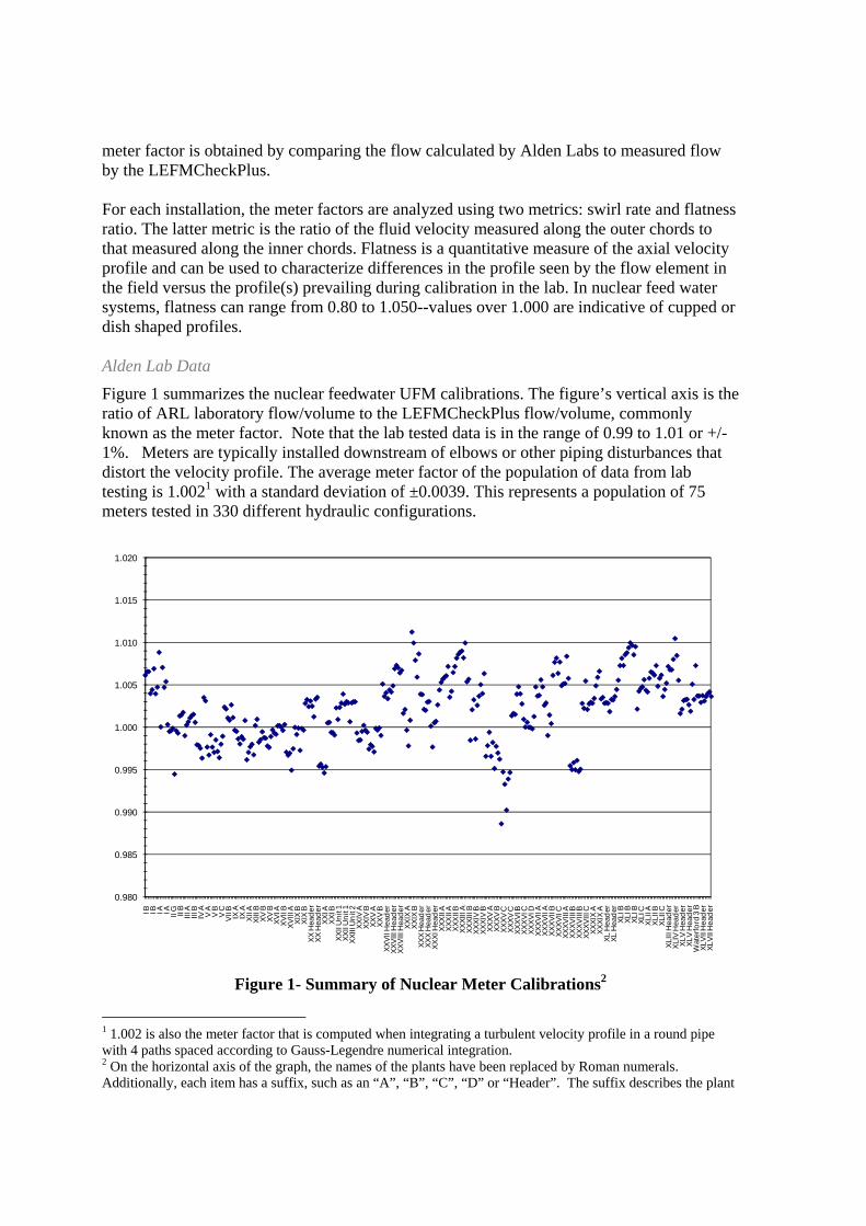
meter factor is obtained by comparing the flow calculated by Alden Labs to measured flow by the LEFMCheckPlus. For each installation, the meter factors are analyzed using two metrics: swirl rate and flatness ratio. The latter metric is the ratio of the fluid velocity measured along the outer chords to that measured along the inner chords. Flatness is a quantitative measure of the axial velocity profile and can be used to characterize differences in the profile seen by the flow element in the field versus the profile(s) prevailing during calibration in the lab. In nuclear feed water systems, flatness can range from 0.80 to 1.050--values over 1.000 are indicative of cupped or dish shaped profiles. Alden Lab Data

Figure 1 summarizes the nuclear feedwater UFM calibrations. The figure’s vertical axis is the ratio of ARL laboratory flow/volume to the LEFMCheckPlus flow/volume, commonly known as the meter factor. Note that the lab tested data is in the range of 0.99 to 1.01 or +/- 1%. Meters are typically installed downstream of elbows or other piping disturbances that distort the velocity profile. The average meter factor of the population of data from lab testing is 1.0021 with a standard deviation of ±0.0039. This represents a population of 75 meters tested in 330 different hydraulic configurations.

0.980

0.985

0.990

0.995

1.000

1.005

1.010

1.015

1.020

I B I B I A I A II G II B

III A

III B

IV A

V A

V B

V C

VII B IX A

IX A

XII A

XIII

BXV

BXV

BXV

I AXV

II B

XVIII

AXI

X B

XIX

BXX

Hea

der

XX H

eade

rXX

I AXX

I BXX

II U

nit 1

XXII

Uni

t 1XX

III U

nit 2

XXIV

AXX

IV B

XXV

AXX

V B

XXVI

I Hea

der

XXVI

II H

eade

rXX

VIII

Hea

der

XXIX

AXX

IX B

XXX

Hea

der

XXX

Hea

der

XXXI

Hea

der

XXXI

I AXX

XII A

XXXI

I BXX

XIII

AXX

XIII

BXX

XIV

BXX

XIV

BXX

XV A

XXXV

BXX

XV C

XXXV

CXX

XVI B

XXXV

I CXX

XVI D

XXXV

II A

XXXV

II A

XXXV

II B

XXXV

II C

XXXV

III A

XXXV

III B

XXXV

III B

XXXV

III C

XXXI

X A

XXXI

X A

XL H

eade

rXL

Hea

der

XLI B

XLI B

XLI B

XLI C

XLII

AXL

II B

XLII

CXL

III H

eade

rXL

IV H

eade

rXL

V H

eade

rXL

V H

eade

rW

ater

ford

3 B

XLVI

I Hea

der

XLVI

I Hea

der

Figure 1- Summary of Nuclear Meter Calibrations2

1 1.002 is also the meter factor that is computed when integrating a turbulent velocity profile in a round pipe with 4 paths spaced according to Gauss-Legendre numerical integration. 2 On the horizontal axis of the graph, the names of the plants have been replaced by Roman numerals. Additionally, each item has a suffix, such as an “A”, “B”, “C”, “D” or “Header”. The suffix describes the plant

Figure 1 reflects the data scatter due to both the differences between individual meters3 and to differences upstream hydraulics.

A typical meter has between 4 to 5 “parametric” calibration tests4 performed. Parametric tests performed to validate/verify the calibration sensitivity can be described in one of three ways, as follows:

Model Component Parametric Tests

The hydraulic model entails the upstream piping including any major hydraulic features that could influence the flow meter’s hydraulics/calibration. This modeling approach has resulted in models that include multiple elbows, venturi(s), valves, Tees, Wyes, reducers etc. In order to validate that the calibration is not sensitive to the model itself, parametric tests are then performed where flow conditioners are installed within the model, to demonstrate the sensitivity, if any, to the construction of the hydraulic model.

Inlet Conditions Parametric Tests

In order to eliminate the possibility that the inlet condition provide by the laboratory influences the calibration itself, the inlet is modified. Modifications include installing and removing plate flow conditioners at the plant model inlet. Occasionally, an eccentric orifice at the inlet has even been installed to demonstrate that even extremely distorted inlet conditions have little effect.

Model Velocity Profile Parametric Tests

To demonstrate that multi-path UFMs with path spacing based on numerical integration of the velocity field are not sensitive to changes in velocity profile, the flatness and/or swirl is intentionally changed. These tests typically use knowledge of the model to increase or decrease the swirl within the system. Sometimes, these changes are accomplished by adding components (for example an eccentric orifice plate) or by changing flow inlet ratios when two or more inlets are entering.

Figures 2, 3 and 4 illustrate some of the complex models of nuclear installations that have been built.

configuration – the letters (“A”, “B”, “C”, and “D”) refer to installations that individual feedwater lines either coming from separate heater chains or going to separate steam generator inlets, while the “Header” refers to applications where the total feedwater goes through one flow meter. 3 Difference include inside diameters ranging from 12 inches to 30 inches. Further, each meter has uncertainties due to dimensional and angle measurement errors and machining differences. 4 A hydraulic test itself includes 5 tests at 5 flowrates that are distributed evenly over a nominal 10:1 flowrate turn down. The flowrates range from a minimum of ~454 m3/hr to the ARL maximum flow rate achievable, nominally 4543 m3/hr. The maximum flowrate depends on the model components that may choked max flow to a slightly lower value.

Figure 2: Example of Calibration with Multiple (Non-Planar) Flow Inlets

Figure 3: Example of Calibration with Non-Planar Model Components with Meter in

Close Proximity to Upstream Elbow (Two meters shown)

Figure 4: Example of Calibration with Meter in Close Proximity to Non-Planar

Coupled Upstream Elbows The data shown in Figure 1 is re-analyzed by subtracting each flowmeter’s average meter factor from its parametric tests to eliminate the geometric uncertainty from the hydraulic uncertainty. The net meter factors are analyzed and graphed below. The standard deviation of the net meter factor due to hydraulic configuration alone is ±0.11%. Throughout this the remainder of this report, the net meter factor data will be considered, unless otherwise stated.

Summary of Nuclear Meter Calibrations

-0.020

-0.015

-0.010

-0.005

0.000

0.005

0.010

0.015

0.020

I B I B I A I A II G

II B

III A

III B

IV A

V A

V B

V C

VII

BIX

AIX

AX

II A

XIII

BX

V B

XV

BX

VI A

XV

II B

XV

III A

XIX

BX

IX B

XX

Hea

der

XX

Hea

der

XX

I AX

XI B

XX

II U

nit 1

XX

II U

nit 1

XX

III U

nit 2

XX

IV A

XX

IV B

XX

V A

XX

V B

XX

VII

Hea

der

XX

VIII

Hea

der

XX

VIII

Hea

der

XX

IX A

XX

IX B

XX

X H

eade

rX

XX

Hea

der

XX

XI H

eade

rX

XX

II A

XX

XII

AX

XX

II B

XX

XIII

AX

XX

III B

XX

XIV

BX

XX

IV B

XX

XV

AX

XX

V B

XX

XV

CX

XX

V C

XX

XV

I BX

XX

VI C

XX

XV

I DX

XX

VII

AX

XX

VII

AX

XX

VII

BX

XX

VII

CX

XX

VIII

AX

XX

VIII

BX

XX

VIII

BX

XX

VIII

CX

XX

IX A

XX

XIX

AX

L H

eade

rX

L H

eade

rX

LI B

XLI

BX

LI B

XLI

CX

LII A

XLI

I BX

LII C

XLI

II H

eade

rX

LIV

Hea

der

XLV

Hea

der

XLV

Hea

der

Wat

erfo

rd 3

BX

LVII

Hea

der

XLV

II H

eade

r

Diff

eren

ce fr

om F

low

met

er's

Ave

rage

MF

Std Dev 0.0011Spread (+/-) 0.0044

Number Meters 75Number Configurations 330

Figure 5: Net Meter Factor for all Calibrations (Net MF = Difference from the flowmeter’s Average MF)

Metrics for Describing Velocity Profile

In each test, the velocity profile of the calibration can be measured. Depending on the hydraulic model, these velocity profiles can range from symmetric to quite distorted (see Figures 6 and 7 as examples of symmetric and distorted).

-0.40

-0.32

-0.24

-0.16

-0.08

0.00

0.08

0.16

0.24

0.32

0.40

0.60

0.65

0.70

0.75

0.80

0.85

0.90

0.95

1.00

1.05

1.10

-1 -0.8 -0.6 -0.4 -0.2 0 0.2 0.4 0.6 0.8 1

Velo

city

Diff

eren

ce (

diffe

renc

e be

twee

n cr

ossi

ng p

aths

)

Norm

aliz

ed V

eloc

ities

Chord Location

Normalized Path Velocities and Velocity Differences

Normalized Velocities Paths 1-4 Normalized Velocities Paths 5-8Normalized Velocities - Average Velocity Difference

Figure 6: Example of Measured Symmetric Velocity Profile

-1.20-1.12-1.04-0.96-0.88-0.80-0.72-0.64-0.56-0.48-0.40-0.32-0.24-0.16-0.080.000.080.160.240.320.400.480.560.640.720.800.880.961.041.121.20

0.400.450.500.550.600.650.700.750.800.850.900.951.001.051.101.151.201.251.301.351.401.451.501.551.60

-1 -0.8 -0.6 -0.4 -0.2 0 0.2 0.4 0.6 0.8 1

Velo

city

Diff

eren

ce (

diffe

renc

e be

twee

n cr

ossi

ng p

aths

)

Norm

aliz

ed V

eloc

ities

Chord Location

Normalized Path Velocities and Velocity Differences

Normalized Velocities Paths 1-4 Normalized Velocities Paths 5-8Normalized Velocities - Average Velocity Difference

Figure 7: Example of Measured Distorted Velocity Profile (due to Swirl) – same meter as in Figure 6

When faced with so many models and their individual velocity profiles, a metric(s) is required to help organize these velocity profiles5. Caldon Ultrasonics defines two metrics, swirl rate and flatness ratio.

Swirl Rate

⎥⎦

⎤⎢⎣

⎡⋅−

⋅−

⋅−

⋅−

=L

37

L

62

S

48

S

51

y2VV

,y2VV

,y2VV

,y2VV

Average Rate Swirl

Where: V1, V4, V5, V8 = Normalized velocities measured along outside/short chords V2, V3, V6, V7 = Normalized velocities measured along inside/long chords yS , yL = Normalized chord location for outside/short and inside/long

paths

Swirl rates computed to be less than 3% are considered to be low and are typically observed in models with only planar connections. Swirl rates greater than 3% are considered “swirling”. Swirl rates greater than 10% are considered to have strong swirl. Figure 8 summarizes the swirl rates observed in model testing.

0

50

100

150

200

250

0 4 8 12 16 20 24 28 32 36 40 44 48 52 56 60 64 68

Num

ber

of T

ests

Con

figur

atio

ns

Swirl (%)

Histogram Swirl Values for All Tests

Figure 8: Swirl Rates Observed in Model Testing

5 It is understood that metrics reduce the fine details of any observed velocity profile into a single number, but this is necessary when comparing so many calibrations.

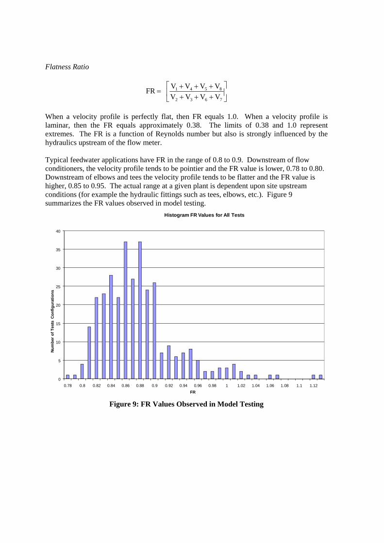
Flatness Ratio

⎥⎦

⎤⎢⎣

⎡++++++

=7632

8541

VVVVVVVV FR

When a velocity profile is perfectly flat, then FR equals 1.0. When a velocity profile is laminar, then the FR equals approximately 0.38. The limits of 0.38 and 1.0 represent extremes. The FR is a function of Reynolds number but also is strongly influenced by the hydraulics upstream of the flow meter. Typical feedwater applications have FR in the range of 0.8 to 0.9. Downstream of flow conditioners, the velocity profile tends to be pointier and the FR value is lower, 0.78 to 0.80. Downstream of elbows and tees the velocity profile tends to be flatter and the FR value is higher, 0.85 to 0.95. The actual range at a given plant is dependent upon site upstream conditions (for example the hydraulic fittings such as tees, elbows, etc.). Figure 9 summarizes the FR values observed in model testing.

0

5

10

15

20

25

30

35

40

0.78 0.8 0.82 0.84 0.86 0.88 0.9 0.92 0.94 0.96 0.98 1 1.02 1.04 1.06 1.08 1.1 1.12

Num

ber

of T

ests

Con

figur

atio

ns

FR

Histogram FR Values for All Tests

Figure 9: FR Values Observed in Model Testing

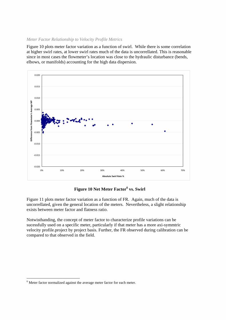
Meter Factor Relationship to Velocity Profile Metrics

Figure 10 plots meter factor variation as a function of swirl. While there is some correlation at higher swirl rates, at lower swirl rates much of the data is uncorrellated. This is reasonable since in most cases the flowmeter’s location was close to the hydraulic disturbance (bends, elbows, or manifolds) accounting for the high data dispersion.

‐0.020

‐0.015

‐0.010

‐0.005

0.000

0.005

0.010

0.015

0.020

0% 10% 20% 30% 40% 50% 60% 70%

Absolute Swirl Rate %

Differen

ce from

 Flowmeter's Average

 MF

Figure 10 Net Meter Factor6 vs. Swirl

Figure 11 plots meter factor variation as a function of FR. Again, much of the data is uncorrellated, given the general location of the meters. Nevertheless, a slight relationship exists between meter factor and flatness ratio. Notwisthanding, the concept of meter factor to characterize profile variations can be sucessfully used on a specific meter, particularly if that meter has a more axi-symmtric velocity profile.project by project basis. Further, the FR observed during calibration can be compared to that observed in the field.

6 Meter factor normalized against the average meter factor for each meter.

‐0.020

‐0.015

‐0.010

‐0.005

0.000

0.005

0.010

0.015

0.020

0.75 0.80 0.85 0.90 0.95 1.00 1.05 1.10 1.15

FR

Differen

ce from

 Flowmeter's Average

 MF

Figure 11 Net Meter Factor vs. FR

Meter Factor Relationship to Diameter

There is no discernable correllation between pipe diameter and meter factor. See Figure 12.

0.980

0.985

0.990

0.995

1.000

1.005

1.010

1.015

1.020

10 15 20 25 30 35

Internal Diameters (inches)

Absolute Meter Factor

Figure 12 Meter Factor vs. Internal Diameter Meter Factor Relationship to Reynolds Number/Flatness Ratio

In determining the meter factor for the flow meter, differences between the laboratory and the field must be considered, particularly the difference in Reynolds number should be considered. At first, the practice was to extrapolate integration uncertainties based on Reynolds Number (Re) from laboratory conditions to the field. This involved extrapolations of Re from laboratory conditions of 1 to 3 million to field conditions Re of 10 to 30 million7. Eventually experience suggested that the measured flatness ratio was a better indication of actual meter performance in the field.

Flatness Ratio Basis

In order to perform this extrapolation a model is developed based on wall law-exponent functions. Symmetrical axial profiles can be described using the inverse power law, which represents the spatial axial velocity distribution in a pipe of circular cross section as follows:

u / U = (y / R)1/n

Where u is local fluid velocity,

U = fluid velocity at the centerline, y = distance from the pipe wall, R = internal radius of the pipe, and n = empirically determined exponent.

The inverse power law was used extensively by Nikuradse and others to fit flow profiles over a wide range of Reynolds Numbers in rough and smooth pipe, in the development of the methodology for calculating friction losses in turbulent flow8. Flatness ratios and meter factors calculated using the power law function are shown in Figure 13.

7 Since the viscosity of the high temperature water (230°C) is significantly less than that of laboratory water (40 to 45°C). 8 Schlichting, Dr. H. Boundary Layer Theory 6th Ed. McGraw-Hill 1968 N.Y. pp563

MF vs. Flatness Ratio - For Smooth Axi-symmetric Velocity Profiles

0.990

0.995

1.000

1.005

1.010

0.80 0.85 0.90 0.95 1.00

FR

MF

Figure 13 Theoretical MF vs. Flatness Ratio

The relationship between meter factor is expressed in the equation MF= -0.0167 FR+ 1.0167. This analysis is better performed on a given meter assuming the flow is axis-symmetric. Example of MF vs. FR Relationship

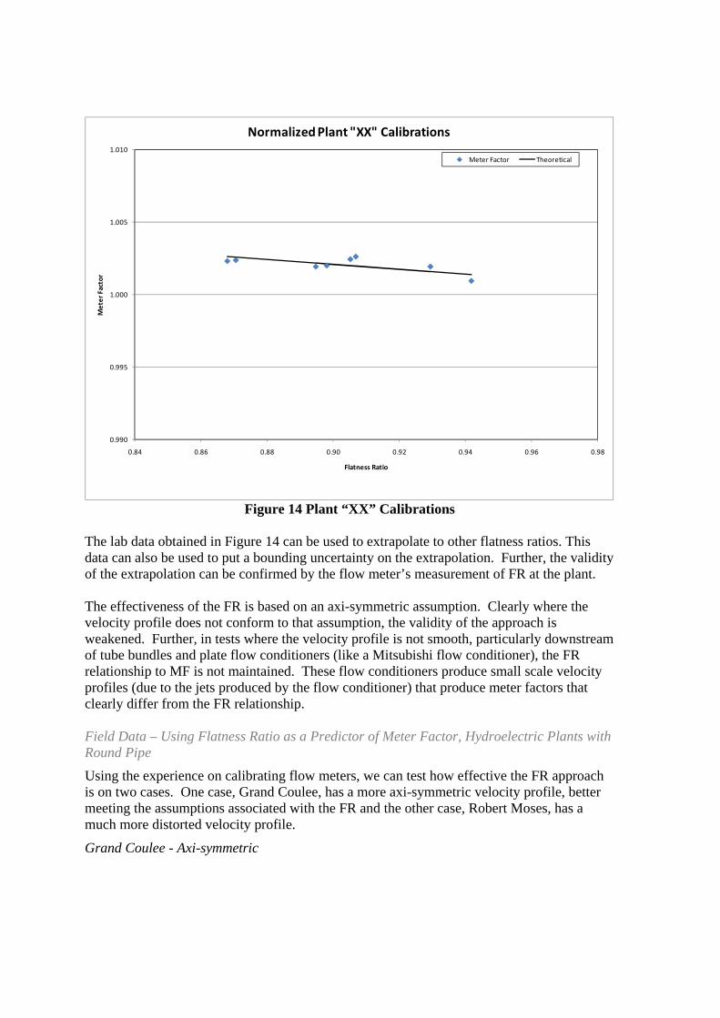
Plant “XX” (see Figure 1) is used to demonstrate the effectiveness of flatness ratio. In Figure 14, the actual data when compared to the theoretical data is very close to the expected value. Figure 14 illustrates the actual meter data along with the theoretical curve (offset to the average of that flowmeter’s meter factor). It should be noted that the piping had sufficient lengths of straight pipe to allow swirl to become axis-symmetric (approximately 10 diameters upstream).

0.990

0.995

1.000

1.005

1.010

0.84 0.86 0.88 0.90 0.92 0.94 0.96 0.98

Meter Factor

Flatness Ratio

Normalized Plant "XX" Calibrations

Meter Factor Theoretical

Figure 14 Plant “XX” Calibrations

The lab data obtained in Figure 14 can be used to extrapolate to other flatness ratios. This data can also be used to put a bounding uncertainty on the extrapolation. Further, the validity of the extrapolation can be confirmed by the flow meter’s measurement of FR at the plant. The effectiveness of the FR is based on an axi-symmetric assumption. Clearly where the velocity profile does not conform to that assumption, the validity of the approach is weakened. Further, in tests where the velocity profile is not smooth, particularly downstream of tube bundles and plate flow conditioners (like a Mitsubishi flow conditioner), the FR relationship to MF is not maintained. These flow conditioners produce small scale velocity profiles (due to the jets produced by the flow conditioner) that produce meter factors that clearly differ from the FR relationship. Field Data – Using Flatness Ratio as a Predictor of Meter Factor, Hydroelectric Plants with Round Pipe

Using the experience on calibrating flow meters, we can test how effective the FR approach is on two cases. One case, Grand Coulee, has a more axi-symmetric velocity profile, better meeting the assumptions associated with the FR and the other case, Robert Moses, has a much more distorted velocity profile.

Grand Coulee - Axi-symmetric

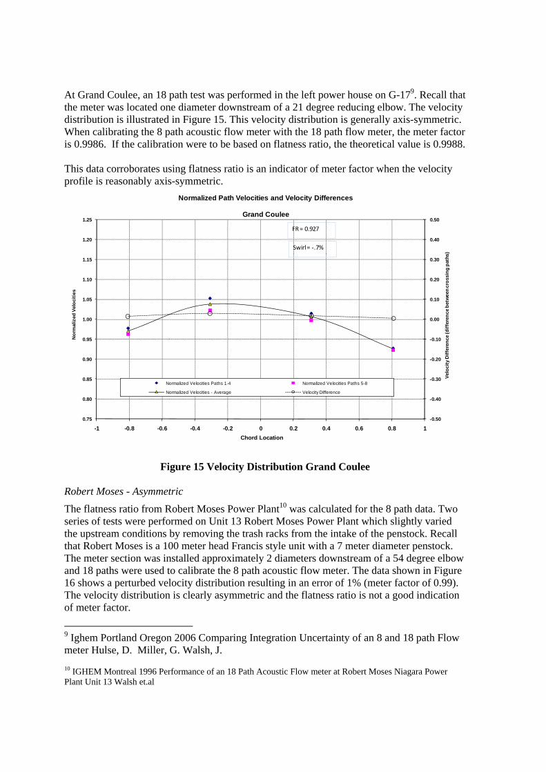
At Grand Coulee, an 18 path test was performed in the left power house on G-179. Recall that the meter was located one diameter downstream of a 21 degree reducing elbow. The velocity distribution is illustrated in Figure 15. This velocity distribution is generally axis-symmetric. When calibrating the 8 path acoustic flow meter with the 18 path flow meter, the meter factor is 0.9986. If the calibration were to be based on flatness ratio, the theoretical value is 0.9988. This data corroborates using flatness ratio is an indicator of meter factor when the velocity profile is reasonably axis-symmetric.

-0.50

-0.40

-0.30

-0.20

-0.10

0.00

0.10

0.20

0.30

0.40

0.50

0.75

0.80

0.85

0.90

0.95

1.00

1.05

1.10

1.15

1.20

1.25

-1 -0.8 -0.6 -0.4 -0.2 0 0.2 0.4 0.6 0.8 1

Velo

city

Diff

eren

ce (d

iffer

ence

bet

wee

n cr

ossi

ng p

aths

)

Nor

mal

ized

Vel

ociti

es

Chord Location

Normalized Path Velocities and Velocity Differences

Grand Coulee

Normalized Velocities Paths 1-4 Normalized Velocities Paths 5-8

Normalized Velocities - Average Velocity Difference

FR = 0.927

Swirl = ‐.7%

Figure 15 Velocity Distribution Grand Coulee

Robert Moses - Asymmetric

The flatness ratio from Robert Moses Power Plant10 was calculated for the 8 path data. Two series of tests were performed on Unit 13 Robert Moses Power Plant which slightly varied the upstream conditions by removing the trash racks from the intake of the penstock. Recall that Robert Moses is a 100 meter head Francis style unit with a 7 meter diameter penstock. The meter section was installed approximately 2 diameters downstream of a 54 degree elbow and 18 paths were used to calibrate the 8 path acoustic flow meter. The data shown in Figure 16 shows a perturbed velocity distribution resulting in an error of 1% (meter factor of 0.99). The velocity distribution is clearly asymmetric and the flatness ratio is not a good indication of meter factor.

9 Ighem Portland Oregon 2006 Comparing Integration Uncertainty of an 8 and 18 path Flow meter Hulse, D. Miller, G. Walsh, J. 10 IGHEM Montreal 1996 Performance of an 18 Path Acoustic Flow meter at Robert Moses Niagara Power Plant Unit 13 Walsh et.al

-0.50

-0.40

-0.30

-0.20

-0.10

0.00

0.10

0.20

0.30

0.40

0.50

0.75

0.80

0.85

0.90

0.95

1.00

1.05

1.10

1.15

1.20

1.25

-1 -0.8 -0.6 -0.4 -0.2 0 0.2 0.4 0.6 0.8 1

Velo

city

Diff

eren

ce (d

iffer

ence

bet

wee

n cr

ossi

ng p

aths

)

Nor

mal

ized

Vel

ociti

es

Chord Location

Normalized Path Velocities and Velocity DifferencesRobert Moses Standard Trash Rack

Normalized Velocities Paths 1-4 Normalized Velocities Paths 5-8

Normalized Velocities - Average Velocity Difference

FR = 0.935

Swirl = ‐1.1%

Figure 16 Robert Moses 8 Path Data

Conclusions A population of 75 flow meters, ranging in inside diameter from 12 inches to 32 inches, was calibrated at an ISO17025 traceable laboratory. 330 different hydraulic configurations were tested. The meter factor population average is 1.002. This average value equals that analytically calculated based on turbulent flow. The meter factor’s sensitivity to upstream hydraulics is ±0.11%. The meter factor variability between meters (excluding the hydraulic) is computed to be ±0.37%. Two metrics, Swirl rate and Flatness ratio are used to describe the different velocity profiles of the calibration population. The meter factor population is slightly correlated to flatness ratio. The correlation to FR is stronger on an individual meter basis, particularly if the meter’s installation has a few diameters upstream to become more axi-symmetric. Use of the FR to determine a meter factor without a calibration is possible, particularly on cases where the hydraulic profile is axi-symmetric, even including swirl. The approach should have more field data to verify its effectiveness.