1

Accuracy of Pressure Sensitive Paint

AIAA Journal, Vol. 39, No.1, January 2001

Tianshu Liu†

† Research Scientist, NASA Langley Research Center

Model Systems Branch, MS 238

Hampton, VA 23681-2199, Member AIAA

and

M. Guille* and J. P. Sullivan‡

* Research Assistant, School of Aeronautics and Astronautics

Purdue University, West Lafayette, IN 47906, Student Member AIAA

‡ Professor, School of Aeronautics and Astronautics

Purdue University, West Lafayette, IN 47906, Member AIAA

2

Abstract

Uncertainty in pressure sensitive paint (PSP) measurement is investigated from a standpoint of

system modeling. A functional relation between the imaging system output and luminescent

emission from PSP is obtained based on studies of radiative energy transports in PSP and

photodetector response to luminescence. This relation provides insights into physical origins of

various elemental error sources and allows estimate of the total PSP measurement uncertainty

contributed by the elemental errors. The elemental errors and their sensitivity coefficients in the

error propagation equation are evaluated. Useful formulas are given for the minimum pressure

uncertainty that PSP can possibly achieve and the upper bounds of the elemental errors to meet

required pressure accuracy. An instructive example of a Joukowsky airfoil in subsonic flows is

given to illustrate uncertainty estimates in PSP measurements.

Introduction

Pressure sensitive paint (PSP) is an optical technique for measuring surface pressure

distributions on wind tunnel models [1-3]. Compared with conventional techniques such as

pressure taps, PSP provides a non-contact way to obtain full-field measurements of surface pressure

with much higher spatial resolution. Due to oxygen quenching of luminescence, luminescent

intensity (I) emitted from PSP is related to air pressure (P) by the Stern-Volmer equation

PK1I

Ip

0 += , (1)

where 0I is the luminescent intensity in the absence of oxygen and pK is the Stern-Volmer

constant. Hence, air pressure can be determined by detecting the luminescent intensity of PSP.

Since 0I is not known in wind tunnel testing, experimental aerodynamicists often use another

version of the Stern-Volmer equation

3

ref

ref

P

P)T(B)T(A

I

I+= , (2)

where refI and refP are the reference luminescent intensity and pressure at a known temperature,

respectively. The coefficients A(T) and B(T), also called the Stern-Volmer constants, are related to

the coefficient pK by refp PK)T(A/)T(B = . Obviously, a constraint is 1)T(B)T(A refref =+ ,

where refT is a reference temperature. The Stern-Volmer equation (2) and its extended forms have

been widely used as operational calibration relations for PSP measurements in aerodynamic tests.

The Stern-Volmer coefficients A(T) and B(T) are temperature-dependent because temperature

affects both non-radiative deactivation and oxygen diffusion in a polymer. The Stern-Volmer

coefficients A(T) and B(T) can be approximately expressed as a linear function of temperature

−+≈

ref

ref

ref

nrref T

TT

RT

E1)A(TA(T) and

−+≈

ref

ref

ref

pref T

TT

RT

E1)B(TB(T) , (3)

where Enr is the Arrhenius activation energy for the non-radiative process, Ep is the activation

energy for oxygen diffusion, and R is the universal gas constant. Eq. (3) implies that the

temperature dependence of A(T) is mainly due to the thermal quenching as temperature sensitive

paint (TSP) while B(T) is related to the temperature dependence of the oxygen diffusivity in a

polymer. For a typical PSP (Bath Ruth + silica gel in GE RTV 118), the coefficients in Eq. (3) are

13.0)T(A ref = , 87.0)T(B ref = , 82.2RT/E refnr = , and 32.4RT/E refp = over a temperature

range from 293K to 333K , where the reference temperature is K298Tref = .

Uncertainty estimates for PSP measurements are highly desirable. Based on the Stern-Volmer

equation, Sajben [4] investigated error sources contributing to the uncertainty of PSP measurements.

He found that the uncertainty strongly depends on flow conditions and surface temperature

4

significantly affects the final measurement result. Oglesby et al. [5] presented an analysis of

intrinsic limits of the Stern-Volmer relation to achievable sensitivity and accuracy. Mendoza [6, 7]

studied CCD camera noise and its effect on PSP measurement and suggested the limiting Mach

number for quantitative PSP measurements. Relevant issues of PSP uncertainty were also addressed

in other literature [1,3,8]. On the other hand, Cattafesta et al. [9] gave uncertainty estimates for

temperature sensitive paint (TSP) measurements with CCD cameras.

The Stern-Volmer equation (1) or (2) describes a generic relationship between air pressure and

luminescent intensity. However, a complete analysis of PSP measurement uncertainty requires a

more specific relation between air pressure and imaging system’s output that depends on various

system elements such as paint, photodetector, optical filters, and illumination sources. In this paper,

solving the transport equations of radiative energy and modeling an imaging system, we obtain a

functional relation between the imaging system’s output and various system parameters such as the

performance parameters of the optical system and the physical properties of PSP. Based on this

relation, a sensitivity analysis is given to evaluate the major elemental error sources and total

uncertainty in PSP measurements. The minimum pressure difference that PSP can resolve is

derived and the upper bounds of the elemental errors for required pressure accuracy are estimated.

A sample uncertainty analysis for subsonic flows over a Joukowsky airfoil is given to illustrate

some issues in PSP measurements.

Luminescent Radiation and Photodetetor Response

Luminescent radiation from a PSP layer on a surface involves two major physical processes.

The first process is absorption of an excitation light through the PSP layer. The incident excitation

light with a wavelength λ1 is absorbed when traveling in the layer, and is reflected and scattered

back to the layer at the wall surface. The second is luminescent radiation that is an absorbing-

5

emitting process in the layer. After luminescent molecules in the layer are excited by the excitation

light, they emit luminescence with a longer wavelength λ2. Figure 1 illustrates absorption and

surface reflection/scattering of an excitation light and radiation of luminescence in a PSP layer. In

general, the illumination and emission processes in a PSP layer can be described by the transport

equations of radiative energy [10,11]. When strong scattering and reflection occur only at the wall

surface, the luminescent intensity emitted from a PSP layer in plane geometry can be analytically

determined by solving the transport equations of radiative energy (see Appendix). When the PSP

layer is optically thin, the outgoing luminescent energy flow rate +2

Q (energy/time/wavelength) on

an area element sA of the PSP paint surface is

AMK)(Eq)TP,(hQ s120 212><=+ Φ , (4)

where is the solid angle, >< M is the coefficient representing the effects of reflection and

scattering of the luminescent light at the wall, 1

is the extinction coefficient of the PSP medium

for the excitation light, h is the paint layer thickness, )TP,(Φ is the luminescent quantum yield

that depends on air pressure and temperature, 0q is the excitation light flux, and )(E 22 is the

luminescence spectrum. The term 1K represents the combined effect of the optical filter for the

excitation light, excitation light scattering, and direction of the incident excitation light. Here, the

extinction coefficient c11

= is a product of the molar absorptivity 1

and luminescent

molecule concentration c . When the PSP layer is optically thick, +2

Q is a non-linear function of

the paint thickness and extinction coefficients. Nevertheless, uncertainty analysis in this case is

essentially the same as that for an optically thin PSP layer.

6

Consider an optical detector system (e.g. CCD camera) shown in Fig. 2. The detector output

depends on not only the outgoing luminescent energy flow rate +2

Q , but also the performance

parameters of the optical system. In Appendix, we obtain an expression for the output of the

detector

2102op

2I KKq)TP,(h

)M(1F

A

4GV

1Φ

+= (5)

where V is the output of the detector, G is the system’s gain, IA is the image area, D/flF = is

the f-number, 12op R/RM = is the optical magnification, fl is the system’s effective focal length,

D is the aperture diameter, 1R is the distance between the lens and the source area (e.g. model

surface), and 2R is the distance between the lens and the sensor. Physically, the term 2K represents

the combined effect of the optical filter for the luminescent light, luminescent light scattering, and

system response to the luminescent light (see Appendix).

Modeling of PSP Measurement System

The detector output is

)TP,(qhV 0fc 1Φ= . (6)

The parameters c and f are 12op

2Ic ])M(1F[AG4)/( −+= and 21f KK= , which are

related to the imaging system performance and filter parameters, respectively. The quantum yield

)TP,(Φ is described by ])O[kkk/(kT)(P, 2qnrrr ++=Φ , where kr is the radiative rate constant,

knr is the non-radiative deactivation rate constant, kq is the quenching rate constant, and [O2] is the

oxygen concentration. This relation reflects the competition among the radiation, non-radiative

deactivation and quenching processes. The concentration of oxygen is related to air pressure P by

Henry’s law PaS]O[ 2 = , where S is the solubility of oxygen and a is the volume fraction of

7

oxygen in air. In PSP applications, the intensity-ratio method is currently used as a typical

procedure to eliminate the effects of spatial variation in illumination, paint thickness, and molecule

concentration. When a ratio between the wind-on and reference wind-off images is taken, air

pressure P can be expressed in terms of the system’s outputs and other variables

B(T)

PA(T)

B(T)

P

),t’V(

)t,(VUP

refrefref1 −=

x’

x. (7)

The factor U1 is

)t,(q

),t’(q

)(c

)c(

)(h

)h(U

ref0

0

refrefreff

f

refc

c1 X

X’

x

x’

x

x’= ,

where Ty)(x,=x and T)y’,(x’=x’ are the coordinates in the wind-off and wind-on images,

respectively, T Z)Y,(X,=X and T)Z’,Y’,(X’=X’ are the object space coordinates in the wind-off

and wind-on cases, respectively, and t and t’ are the instants at which the wind-off and wind-on

images are taken, respectively. Here the paint thickness and dye concentration are expressed as a

function of x rather than X because image registration errors are more easily treated in the image

plane. In fact, x and X are related through the perspective collinearity equations in

photogrammetry.

In order to separate complicated coupling between the temporal and spatial variations of the

variables, some terms in (7) can be further decomposed when a small model deformation and a short

time interval are considered. The wind-on image coordinates can be expressed as a superposition of

the wind-off coordinates and displacement vector, i.e., xxx’ += . Similarly, the time

decomposition is ttt +=’ . For small x and t , the ratio of the images can be separated into

two factors, ),t’)/V(t,(Vref x’x )t,)/V(t,(V)(D)t(D refxt xxx≈ , where the factor

8

VW��)(t/V(1)W(Dt ∂∂−= and V)()V(1)(Dx /xx •∇−= represent the effects of the

temporal and spatial changes of the luminescent intensity, respectively. The temporal change of the

luminescent intensity is mainly caused by photodegradation and sedimentation of dusts and oil

droplets on a surface. The spatial intensity change is due to model deformation. In the same

fashion, the excitation light flux is decomposed into ≈)t,()/q,t’(q ref00 XX’

)t,()/qt,(q)t(D ref00q0 XX’ , where the factor ref00q0 q/W�)(t/q(1)W(D ∂∂+= reflects the

temporal variation in the excitation light flux. The use of the above estimates yields the modified

Stern-Volmer equation

B(T)

PA(T)

B(T)

P

)t,V(

)t,(VUP

refrefref2 −=

x

x. (8)

where

)t,(q

)t,(q

)(c

)c(

)(h

)h()t(D)(D)t(DU

ref0

0

refrefreff

f

refc

cq0xt2 X

X’

xx’

xx’

x= .

Without model motion ( xx’ = and XX’ = ) and temporal illumination fluctuation, the factor U2 is

unity and then Eq. (8) recovers the generic Stern-Volmer equation. However, unlike the generic

Stern-Volmer equation used in previous PSP uncertainty estimates, Eq. (8) is a general relation that

includes the effects of model deformation, spectral variability, and temporal variations in both

illumination and luminescence. This relation allows a more complete uncertainty analysis and a

clearer understanding of how these variables contribute the total uncertainty in PSP measurements.

Error Propagation, Sensitivity and Total Uncertainty

According to general uncertainty analysis formalism [12,13], the total uncertainty of pressure P

is described by the error propagation equation

9

ji

1/2ji

ji

M

1ji,

ji2

)]var()var([SS

P

(P)var ∑=

= , (9)

where 1/2jijiji )]var()var()/[cov(= is the correlation coefficient between the variables

i and j , ><= 2ii )(var and ><= jiji )(cov are the variance and covariance,

respectively, and the notation >< denotes the statistical assemble average. Here the variables

M}1i,{ i L= denote a set of the parameters )t(Dt , )(Dx x , )t(Dq0 , V , refV , refcc / ,

refff / , refh/h , refc/c , ref00 /qq , refP , T , A, and B. The sensitivity coefficients iS are defined

as )/P)(/P(S iii ∂∂= . Eq. (9) becomes particularly simple when the cross-correlation

coefficients between the variables vanish ( ji,0ji ≠= ). Table I lists the sensitivity coefficients,

the elemental errors and their physical origins. Many sensitivity coefficients are proportional to a

factor )P/(P//B(T)][A(T)1 ref+ . For Bath Ruth + silica-gel in GE RTV 118, Figure 3 shows the

factor )P/(P//B(T)][A(T)1 ref+ as a function of refP/P for different temperatures. This factor is

only slightly changed by temperature. The temperature sensitivity coefficient is

=TS )T(B/P]/P(T)A’(T)[B’T ref+− , where the prime denotes differentiation. Figure 4 shows

the absolute value of TS as a function of refP/P at different temperatures. As long as the

elemental errors are evaluated, the total uncertainty in pressure can be calculated using Eq. (9). The

major elemental error sources will be discussed below.

Elemental Error Sources

Photodetector noise and limiting pressure resolution

The uncertainties in the photodetector outputs V and refV are contributed from various noise

sources in a photodetector (e.g. camera) such as photon shot noise, dark current shot noise, amplifier

10

noise, quantization noise, and pattern noise. When the dark current and pattern noise are subtracted

and the noise floor is negligible, the detector noise is photon-shot-noise-limited. In this case, the

signal-to-noise ratio (SNR) of the detector is 2/1d )%G/V(SNR h= , where is the Planck’s

constant [Js], ν is the frequency [s-1], Bd is the electrical bandwidth [s-1] of the detection electronics,

G is the system’s gain, and V is the detector output. The uncertainties in the outputs are

dBGVvar(V) h= and drefref BGV)var(V h= . In the photon-shot-noise-limited case in which the

error propagation equation contains only two terms related to V and refV , the uncertainty in P is

2/1

ref

ref

2/1

ref

d

P

P)T(B)T(A1

P

P

)T(B

)T(A1

V

BG

P

P

++

+

= h

. (10)

This relation holds for both non-imaging detectors and CCD. For a CCD camera, the first factor in

the right-hand side of Eq. (10) can be simply expressed by the total number of photoelectrons

collected over the integration time ( dB/1∝ ) )%G/(Vn dpe h= . When the full-well capacity of a

CCD is achieved, one obtains the minimum pressure difference that PSP can measure from a single

frame of image

1/2

ref

ref

maxrefpe

min

P

PB(T)A(T)1

P

P

B(T)

A(T)1

)(n

1

P

3�(

++

+= , (11)

where maxrefpe )(n is the full-well capacity of a CCD in reference conditions. When N images are

averaged, the limiting pressure difference (11) is further reduced by a factor N1/2. Eq. (11) provides

an estimate for the noise-equivalent pressure resolution for a CCD camera. When maxrefpe )(n is

500,000 electrons and Bath Ruth + silica-gel in GE RTV 118 is used, the minimum pressure

uncertainty P/3�( min is shown in Fig. 5 as a function of refP/P for different temperatures. It is

11

indicated that an increasing temperature degrades the limiting pressure resolution. Figure 6 shows

P/3�()(n minmaxrefpe as a function of refP/P for different values of the Stern-Volmer

coefficient B(T) . Clearly, a larger B(T) leads to a smaller limiting pressure uncertainty

P/3�( min .

Errors induced by model deformation

Model deformation due to aerodynamic loads causes a displacement xx’x −= of the wind-

on image relative to the wind-off image. This displacement leads to the deviations of )(Dx x ,

refh/h , refc/c , and ref00 /qq in Eq. (8) from unity because the distributions of the luminescent

intensity, paint thickness and dye concentration are not spatially homogeneous on a surface. After

the image registration is applied to align the images, the estimated variances are

2x V/)V(W)](var[D ≈x , 2

refref )h/()h(W)h/hvar( ≈ , and 2refref )c/()c(W)c/cvar( ≈ . The

operator )W( • is defined as ( ) ( ) 2y

22x

2 y/x/)W( ∂∂+∂∂=• , where x and y are the standard

deviations of least-squares estimation in the image registration.

The uncertainty in )()/q(q ref00 X’X is caused by a change in the illumination intensity on a

model surface after the model moves with respect to the light sources. When a point on the model

surface travels along the displacement vector XX’X −= in object space, the variance of

ref00 /qq is estimated by 2

02

ref0ref00 )()q()q()](q/)([qvar XX’X •− ∇≈ . Consider a point light

source with a light flux distribution n

ss0 -)-(q−= XXXX , where n is an exponent (normally n =

2) and sX-X is the distance between the point X on the model surface and the light source

location sX . The variance of ref00 /qq for the single point source is )](q/)([qvar ref00 X’X

12

242 )()(n XX-XX-X ss •−= . The variance for multiple point light sources can be obtained

based on the principle of superposition. In addition, model deformation leads to a small change in

the distance between the model surface and the camera lens. The uncertainty in the camera

performance parameters due to this change is ≈)/var( refcc2

112

212 )/RR()]R/(RR[ + , where

1R is the distance between the lens and the model surface and 2R is the distance between the lens

and the sensor. For 21 RR >> , this error is very small.

Temperature effects

Since the luminescent intensity of PSP is intrinsically temperature-dependent, a temperature

change on a model surface during wind tunnel runs results in a bias error in PSP measurement if the

temperature effects are not corrected. Temperature also influences the total uncertainty of PSP

measurement by altering the sensitivity coefficients of the variables in the error propagation

equation. Hence, the surface temperature on a model must be known in order to correct the

temperature effects of PSP. In general, the surface temperature distribution can be either measured

by using temperature sensitive paint (TSP) or determined numerically by solving the energy

equation in flows coupled with the heat conduction equation in the model. For a compressible

boundary layer on an adiabatic wall, the adiabatic wall temperature awT can be estimated using a

simple relation 1220aw ]2/1)M-(1[]2/1)M-(r1[T/T −++= γγ , where r is the recovery factor

for the boundary layer, 0T is the total temperature, M is the local Mach number, and γ is the

specific heat ratio.

PSP calibration errors

The uncertainties in determining the Stern-Volmer coefficients A(T) and B(T) are calibration

errors. In a priori PSP calibration in a pressure chamber, the uncertainty is represented by the

13

standard deviation of data collected in replication tests. Because the tests in a pressure chamber are

well controlled, a priori calibration result shows a small precision error. However, a significant

bias error is usually found when the a priori calibration result is directly used for data reduction in

wind tunnel tests. In contrast, in-situ calibration utilizes pressure tap data over a model surface to

determine the Stern-Volmer coefficients. Because the in-situ calibration fits the local luminescent

intensity to the pressure tap data, it can to some extent reduce bias errors such as the temperature

effects and naturally achieves a better agreement with the pressure tap data.

Temporal variations in luminescence and illumination

For PSP measurements in steady flows, a temporal change in the luminescent intensity mainly

results from the photodegradation and sedimentation of dusts and oil droplets on a model surface.

The photodegradation of PSP may occur when there is a considerable exposure of PSP to the

excitation light between the wind-off and wind-on measurements. Dusts and oil droplets in air

sediment on a model surface during wind-tunnel runs. The resulting dust/oil layer absorbs both the

excitation light and luminescent emission on the surface and thus causes a decrease of the

luminescent intensity. The uncertainty in )t(Dt due to these effects can be collectively

characterized by the variance 2t ]VW��)(t/V[()]W(var[D ∂∂≈ . Similarly, the uncertainty in

)t(Dq0 , which is produced by an unstable excitation light source, is described by

2ref00q0 ]qW��)(t/q[()]W(var[D ∂∂≈ .

Spectral variability and filter leakage

The uncertainty in refff / is mainly attributed to the spectral variability in the illumination

light and spectral leaking of the filters. The spectral variability between flashes of a xenon lamp has

been observed [14]. The uncertainties in the absolute pressure and pressure coefficient due to the

14

flash spectral variability are 0.05 psi and 0.01, respectively. If the optical filters are not selected

appropriately, a small portion of photons from the excitation light and ambient light may reach the

detector through the filters. This spectral leakage produces an additional output to the luminescent

signal.

Pressure mapping errors

The uncertainties in pressure mapping are related to the data reduction procedure in which PSP

data in 2D images are mapped onto a model surface grid in 3D object space. They include errors in

camera calibration and mapping onto a surface grid of a presumed rigid body. The camera

calibration error is represented by the standard deviations x and y of the calculated target

coordinates from the measured target coordinates in the image plane. Typically, a good camera

calibration method gives the standard deviation of about 0.04 pixels. For a given PSP image, the

pressure variance induced by the camera calibration error is ( ) ( ) 2y

22x

2 y/Px/Pvar(P) ∂∂+∂∂≈ .

The pressure mapping onto a non-deformed surface grid leads to another deformation-related

error since the model undergoes considerable deformation due to aerodynamic loads in wind tunnel

tests. If a displacement vector of a point on the model surface in object space is XX’X −= , the

pressure variance induced by mapping onto a rigid body grid without correcting the deformation is

2

surfsurf )()P()(Pvar X•∇= , where surf)P(∇ is the pressure gradient on the surface and surf)( X

is the component of the displacement vector projected on the surface. To eliminate this error, a

deformed surface grid has to be generated for PSP mapping based on model deformation

measurements [15].

Other error sources

15

Other error sources include self-illumination, paint intrusiveness, limiting time response, and

induction effect. Self-illumination is a phenomenon that luminescence from one part of a model

surface reflects to another surface, thus distorting the observed luminescent intensity by superposing

all the rays reflected from other points. It often occurs on surfaces of neighbor components of a

complex model. Ruyten [16] discussed this problem and gave a numerical correction procedure for

self-illumination. Paint layer with a non-homogenous thickness modifies the shape of a model such

that the surface pressure distribution may be changed. Hence, this paint intrusiveness to flows

should be considered as an error source in PSP measurements. In PSP applications in unsteady

flows, the limiting time response of PSP imposes an additional restriction on the accuracy of PSP

measurement. The time response of PSP is mainly determined by oxygen diffusion process through

the PSP layer [17]. Another problem related to the time response is the ‘induction effect’ defined as

an increase in luminescence during the first few minutes of illumination. This effect has been

observed with certain paints and the photochemical process behind it has been explained by

Gouterman [18].

Allowable Upper Bounds of Elemental Errors

In the design of PSP experiments, we need to give the allowable upper bounds of the elemental

errors for required pressure accuracy. This is an optimization problem subject to constraints. In

matrix notations, Eq. (9) is expressed as AT=2P , where 22

P (P)/Pvar= , jijiij SSA = , and

i1/2

ii /])var([= . For a required pressure uncertainty P , we look for a vector up to

maximize an objective function W T=H , where W is the weighting vector. The vector up

gives the upper bounds of the elemental errors for a given pressure uncertainty P . The use of the

16

Lagrange multiplier method requires )(H 2P AW TT −+= to be maximal, where λ is the

Lagrange multiplier. The solution to this optimization problem gives the upper bounds

P1/21 )( WAW

WAT

1

up −

−

= . (12)

For the uncorrelated variables with j)(i0ji ≠= , Eq. (12) reduces to

1/2

k

2k

2kPi

2ii WSWS)(

−−−

= ∑up . (13)

When the weighting factors iW equal the absolute values of the sensitivity coefficients |S| i , the

upper bounds can be expressed in a very simple form

1i

2/1VPi SN/)( −−=up , ( VN,,2,1i L= ) (14)

where VN is the total number of the variables or the elemental error sources. The relation (14)

clearly indicates that the allowable upper bounds of the elemental uncertainties are inversely

proportional to the sensitivity coefficients and the square root of the total number of the elemental

error sources. Figure 7 shows a distribution of the upper bounds of 15 variables for Bath Ruth +

silica-gel in GE RTV 118 at 8.0P/P ref = and K293T = . Clearly, the allowable upper bound for

temperature is much lower than others. Therefore, the temperature effcts must be tightly controlled

in order to achieve the required pressure accuracy.

PSP Uncertainty Estimates on a Joukowsky Airfoil in Subsonic Flows

Hypothetical PSP measurements on a Joukowsky airfoil in subsonic flows are considered to

illustrate how to estimate the elemental errors and the total uncertainty by using the techniques

developed above. The airfoil and incompressible potential flows around it are generated by using

the Joukowsky transform. The pressure coefficients Cp on the airfoil in the corresponding

17

compressible flows are obtained by using the Karman and Tsien rule. Figure 8 shows typical

distributions of the pressure coefficient and adiabatic wall temperature on the Joukowsky airfoil at

Mach 0.5.

Presumably, Bath Ruth + silica-gel in GE RTV 118 is used, which has the Stern-Volmer

coefficients ]T/)TT(82.21[0.13A(T) refref−+≈ and ]T/)TT(32.41[0.87B(T) refref−+≈

(293K < T < 333K). The uncertainties in a priori PSP calibration are 1%%�%/AA == . Assume

that the spatial changes of the paint thickness and dye concentration in the image plane are

0.5%/pixel and 0.1%/pixel, respectively. The rate of the photodegradation of the paint is 0.5%/hour

for a given excitation level and the exposure time of the paint is 60 seconds between the wind-off

and wind-on images. The rate of reduction of the luminescent intensity due to dust/oil

sedimentation on the surface is assumed to be 0.5%/hour.

In an object-space coordinate system whose origin is at the leading edge of the airfoil, four light

sources for illuminating PSP are placed at the locations )c3,c-(s1 =X , )c3,c2(s2 =X ,

)c3,c-(s3 −=X , and )c3,c2(s4 −=X , where c is the chord of the airfoil. For the light sources

with unit strength, the illumination flux distributions on the upper and lower surfaces are,

respectively, 2

s2

2

s1up0 --)(q−−

+= XXXX upup and 2

s42

s3low0 --)(q−− += XXXX lowlow ,

where upX and lowX are the coordinates of the upper and lower surfaces of the airfoil, respectively.

The temporal variation of irradiance of the lights is assumed to be 1%/hour. It is also assumed that

the spectral leakage of the optical filters for the lights and cameras is 0.3%. Two cameras, viewing

the upper surface and lower surface respectively, are located at )c4/2,c( and )c4/2,c( − .

18

The uncertainty associated with the shot noise can be estimated by using Eq. (10). Assume that

the full-well capacity of 350,000)n( maxpe = electrons of a CCD camera is utilized. The numbers

of photoelectrons collected in the CCD camera are mainly proportional to the distributions of the

illumination fields on the model surfaces. Thus, the photoelectrons on the upper and lower surfaces

are estimated by ])qmax[(/)q()n()n( up0up0maxpeuppe = and

])qmax[(/)q()n()n( low0low0maxpelowpe = . Combination of these estimates and Eq. (10) can give

the shot-noise-generated uncertainty distributions on the surfaces.

Movement of the airfoil produced by aerodynamic loads can be expressed by a superposition of

local rotation (twist) and translation. The transformation between the non-moved and moved

surface coordinates T)Y,X(=X and T)’Y,’X(=X’ is TXRX’ += )( twistθ , where )( twistθR is

the rotation matrix, twistθ is the local wing twist, and T is the translation vector. Here, for

otwist 1−=θ and T)c01.0,c001.0(=T , the uncertainty in )()/q(q ref00 X’X is estimated by

20

2ref0ref00 )()q()q()](q/)([qvar XX’X •

− ∇≈ , where the displacement vector is XX’X −= .

The pressure variance associated with mapping onto a rigid body grid without correcting the

deformation is estimated by 2

surfsurf )()P()(Pvar X•∇= , where surf)P(∇ is the pressure gradient

on the surface and surfsurf X)X’X) −= (( is the component of the displacement vector projected

on the surface.

To estimate the temperature effects, an adiabatic model is considered at which the wall

temperature awT is 1220aw ]2/1)M-(1[]2/1)M-(r1[T/T −++= γγ . The recovery factor is r =

0.843 for a laminar boundary layer. Assuming that the reference temperature refT equals to the total

19

temperature K293T0 = , one can calculate the temperature difference refaw TTT −=∆ between the

wind-on and wind-off cases (Fig. 8).

The total uncertainty in air pressure P is estimated by substituting all the elemental errors into

Eq. (9). Figure 9 shows the pressure uncertainty distributions on the upper and lower surfaces of the

airfoil for different freestream Mach numbers. It is indicated that the temperature effects of PSP

dominate the uncertainty of PSP measurement in an adiabatic wall. The uncertainty becomes larger

and larger as Mach number increases since the adiabatic wall temperature increases. The local

pressure uncertainty on the upper surface is as high as 50% at one location for Mach = 0.7, which is

caused by the local surface temperature change of about 6 degrees. In order to compare the PSP

uncertainty with the pressure variation on the airfoil, a maximum relative pressure variation on the

airfoil is defined as p2

surfCmaxM5.0P/3max ∆γ ∞∞ = . Figure 10 shows the maximum relative

pressure variation ∞P/3maxsurf

along with the chord-averaged PSP uncertainty

awPSP3�3�( >< on the adiabatic airfoil at Mach numbers ranging from 0.05 to 0.7. The

uncertainty 0TPSP3�3�( =>< ∆ without the temperature effects is also plotted in Fig. 10, which is

mainly dominated by the a priori PSP calibration error 1%%�% = in this case. The curves

∞P/3maxsurf

, awPSP3�3�( >< and 0TPSP3�3�( =>< ∆ intersect near Mach 0.1. When the

PSP uncertainty exceeds the maximum pressure variation on the airfoil, the pressure distribution on

the airfoil cannot be measured by PSP. In general, because of a smaller temperature change on a

non-adiabatic wall, the PSP uncertainty for a real wind tunnel model falls into the shadowed region

confined by awPSP3�3�( >< and 0TPSP3�3�( =>< ∆ (see Fig. 10). The PSP uncertainty

associated with the shot noise ShotNoisePSP3�3�( >< is also plotted in Fig. 10. The intersection

20

between ∞P/3maxsurf

and ShotNoisePSP3�3�( >< gives the limiting low Mach number ( 06.0~ )

for PSP application. The uncertainties in the lift ( LF ) and pitching moment ( cM ) can also be

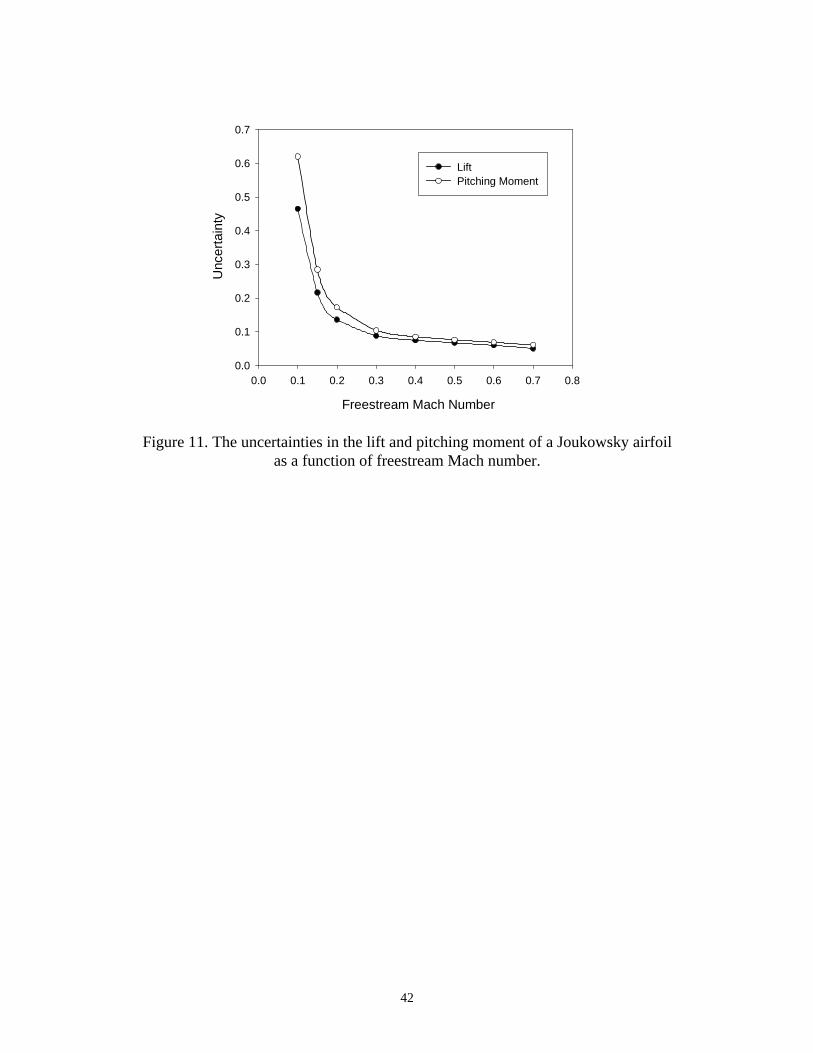
calculated from the PSP uncertainty distribution on the surface. Figure 11 shows the uncertainties

in the lift and pitching moment relative to the leading edge for the Joukowsky airfoil at different

Mach numbers when the angle of attack is 4 degrees. The uncertainties in the lift and moment

decrease monotonously as Mach number increases because the absolute values of the lift and

moment rapidly increase with Mach number.

Conclusions

Based on more rigorous PSP system modeling, a general framework is built in which the

physical origins of the elemental error sources are clearly identified and their contributions to the

total uncertainty are systematically evaluated. For a required pressure uncertainty, the allowable

upper bounds of the elemental errors are given by a simple formula, which are inversely

proportional to the sensitivity coefficients. Among the major elemental error sources, for a typical

PSP, temperature has the largest sensitivity coefficient and the lowest allowable upper bound of

error in PSP measurements. Therefore, the temperature effects must be corrected in order to obtain

quantitative pressure results. The minimum pressure uncertainty limited by the photon-shot-noise

can be described by an analytical expression, which is related to the Stern-Volmer coefficients, local

air pressure and the number of photoelectrons. The shot-noise-limited PSP uncertainty increases

with temperature and decreases as the Stern-Volmer coefficient B(T) increases. The sample

uncertainty analysis on a Joukowsky airfoil in subsonic flows further confirms that the temperature

effects dominate the PSP measurement uncertainty. It is enlightening to compare the uncertainties

in several different conditions (on the adiabatic wall, without the temperature effects, and in the

21

shot-noise-limited case) with the maximum relative pressure change on the surface as a function of

freestream Mach number. This comparison not only shows the uncertainties relative to the surface

pressure change, but also gives the limiting low Mach number for PSP measurements.

Acknowledgments

The authors would like to thank the reviewers for their constructive comments.

22

References

[1] Crites, B. C., “Measurement Techniques Pressure Sensitive Paint Technique,” Lecture Series

1993-05, von Karman Institute for Fluid Dynamics, 1993.

[2] McLachlan, B. G. and Bell, J. H., “Pressure-Sensitive Paint in Aerodynamic Testing,”

Experimental Thermal and Fluid Science, 10, 1995, pp. 470-485.

[3] Liu, T., Campbell, B. T., Burns, S. P. and Sullivan, J. P., “Temperature- and Pressure-Sensitive

Luminescent Paints in Aerodynamics,” Applied Mechanics Reviews, Vol. 50, No. 4, 1997, pp.

227-246.

[4] Sajben, M., “Uncertainty Estimates for Pressure Sensitive Paint Measurements,” AIAA J., Vol.

31, No. 11, 1993, pp. 2105-2110.

[5] Oglesby, D. M., Puram, C. K. and Upchurch, B. T., “Optimization of Measurements with Pressure

Sensitive Paints,” NASA TM 4695, 1995.

[6] Mendoza, D. R., “An Analysis of CCD Camera Noise and its Effect on Pressure Sensitive Paint

Instrumentation System Signal-to-Noise Ratio,” ICIASF ’97 Record, International Congress on

Instrumentation in Aerospace Simulation Facilities, Pacific Grove, CA, September 29-October 2,

1997, pp. 22-29.

[7] Mendoza, D. R., “Limiting Mach Number for Quantitative Pressure-Sensitive Paint

Measurements,” AIAA J., Vol. 35, No. 7, 1997, pp. 1240-1241.

[8] Morris, M. J., Benne, M. E., Crites, R. C. and Donovan, J. F., “Aerodynamics Measurements

Based on Photoluminescence,” AIAA Paper 93-0175, Jan. 1993.

[9] Cattafesta, L., Liu, T., and Sullivan, J., “Uncertainty Estimates for Temperature Sensitive Paint

Measurements with CCD Cameras,” AIAA J., Vol. 36, No. 11, 1998, pp. 2102-2108.

[10] Pomraning, G. C., “Radiation Hydrodynamics,” Pergamon Press, New York, 1973, pp. 10-49.

23

[11] Modest, M. F., “Radiative Heat Transfer,” McGraw-Hill, Inc., New York, 1993, pp. 295-320.

[12] Ronen, Y., “Uncertainty Analysis,” CRC Press, Inc., Boca Raton, Florid, 1988, pp. 2-39.

[13] Bevington, P. R. and Robinson, D. K., “Data Reduction and Error Analysis for the Physical

Sciences (Second Edition),” McGraw-Hill, Inc., New York, 1992, pp. 38-48.

[14] Possolo, A. and Maier, R., “Gauging Uncertainty in Pressure Measurement Due to Spectral

Variability of Excitation Illumination,” Proceeding of the Sixth Annual Pressure Sensitive Paint

Workshop, The Boeing Company, Seattle, Washington, October 6-8, 1998, pp. 15-1 to 15-12.

[15] Liu, T., Radeztsky, R., Garg, S., and Cattafesta, L., “A Videogrammetric Model Deformation

System and its Integration with Pressure Paint,” AIAA Paper 99-0568, Jan. 1999.

[16] Ruyten, W. M., “Correcting Luminescent Paint Measurements for Self-Illumination,” ICIASF

’97 Record, International Congress on Instrumentation in Aerospace Simulation Facilities, Pacific

Grove, CA, September 29-October 2, 1997, pp. 3-9.

[17] Carroll, B. F., Abbitt, J. D., Lukas, E. W. and Morris, M. J., “Step Response of Pressure

Sensitive Paints,” AIAA J., Vol. 34, No. 3, 1996, pp. 521-526.

[18] Gouterman, M., “Oxygen Quenching of Luminescence of Pressure-Sensitive Paint for Wind

Tunnel Research,” Journal of Chemical Education, Vol. 74, No. 6, 1997, pp. 1-7.

Appendix: Luminescent Radiation from PSP and Photodetector Output

Luminescent radiation from a pressure sensitive paint (PSP) on a surface involves two major

physical processes. The first process is absorption of an excitation light through a PSP layer. The

second is luminescent radiation that is an absorbing-emitting process in the layer. These processes

can be described by the transport equations of radiative energy [10, 11]. The luminescent intensity

emitted from a PSP layer in plane geometry will be analytically determined by solving the transport

equations and the corresponding photodetector output will be derived.

24

Excitation light

Consider a PSP layer with a thickness h on a wall (Figure 1). Suppose that PSP is not a

scattering medium and scattering exists only at the wall surface. An incident excitation light beam

with a wavelength λ1 enters the layer. Without scattering and other sources for excitation energy,

the incident light is attenuated by absorption through a PSP medium. In plane geometry where the

radiative intensity is independent of the azimuthal angle, the intensity of the incident excitation light

with λ1 can be described by

0Izd

Id11

1 =+ −−

, (A1)

where −1

I is the incident excitation light intensity, cos= is the cosine of the polar angle , and

1 is the extinction coefficient of the PSP medium for the incident excitation light with λ1. The

extinction coefficient c11

= is a product of the molar absorptivity 1

and luminescent

molecule concentration c . Here, the intensity is defined as radiative energy transferred per unit

time, solid angle, spectral variable and area normal to the ray. The superscript ‘-‘ in −1

I indicates

the negative direction in which the light enters the layer. The incident angle ranges from 2/ to

3 /2 ( 01 ≤≤− ) (see Fig. 1). For the collimated excitation light, the boundary value for Eq. (A1)

is the component penetrating into the PSP layer,

)�)(Eq)1(h)(zI ex10ap

111−−==− , (A2)

where 0q and )(E 11 are the radiative flux and spectrum of the incident excitation light,

respectively, ap

1 is the reflectivity of the air-PSP interface, ex is the cosine of the incident angle

of the excitation light, and )� is the Dirac-delta function. The solution to Eq. (A1) is

25

z)](h�/[(exp)�)(Eq)1(I1111 ex10

ap −−−=− . ( 01 ≤≤− ) (A3)

This relation describes the decay of the incident excitation light intensity through the layer. The

incident excitation light flux at the wall integrated over the ranges of from either to 2/ or

to 3 /2 is

),(Eq)1(Cd0)(zI)0z(q 10ap

d

0

1- 1111−≅=−== ∫ −− (A4)

where dC is the coefficient representing the directional effect of the excitation light, that is,

)/h(expC exexd 1−= . ( 01 ex ≤≤− ) (A5)

When the incident excitation light impinges on the wall, the light reflects and re-enters into the

layer. Without scattering source inside PSP, the intensity of the reflected and scattered light from

the wall is described by

0Izd

Id11

1 =+ ++

, (A6)

where +1

I is the intensity in the positive direction emanating from the wall. As shown in Fig. 1, the

range of µ is 10 ≤≤ ( /20 ≤≤ and 02/- ≤≤ ) for the outgoing reflected and scattered

light. The superscript ‘+’ indicates the outgoing direction from the wall. For the wall that reflects

diffusely, the boundary condition for Eq. (A6) is

),(Eq)1(C)0z(q0)(zI 10apwp

dwp

111111−==== −+ (A7)

where wp

1 is the reflectivity of the wall-PSP interface for the excitation light. The solution to Eq.

(A6) is

) 1(0��/z(exp)(Eq)1(CI11111 10

apwpd ≤≤−−=+ µ (A8)

26

At a point inside the PSP layer, the net excitation light flux is contributed by the incident and

scattering light rays from all the possible directions. The net flux is calculated by adding the

incident flux (integrated over /2to= and /23to= ) and scattering flux (integrated over

/2to0= and /2to0 −= ). The net flux is

.2)]/z3(exp)/z(exp[)(Eq)1(C

dI2dI2)q(

11111

111

wpex10

apd

0

1

0

1net

−+−−≅

−−= ∫∫ +

−

−

(A9)

Note that the derivation of Eq. (A9) uses the approximation of the exponential integral of third

order, 2)/x3(exp(1/2)(x)E3 −≅ .

Luminescent emission

After luminescent molecules in PSP absorb the energy from the excitation light with a

wavelength λ1, they emit luminescence with a longer wavelength λ2 due to the Stokes shift.

Luminescent radiative transfer in PSP is an absorbing-emitting process. The luminescent light rays

from the luminescent molecules radiate in both the inward and outward directions.

For the luminescent emission toward the wall, the luminescent intensity −2

I can be described by

(z)SIzd

Id222

2 =+ −−

, ( 01 ≤≤− ) (A10)

where (z)S2

is the luminescent source term and the extinction coefficient c22

= is a product

of the molar absorptivity 2

and luminescent molecule concentration c . The luminescent source

term (z)S2

is assumed to be proportional to the extinction coefficient for the excitation light, the

quantum yield, and the net excitation light flux filtered over a spectral range of absorption. A model

for the luminescent source term is expressed as

27

∫∞

=0

111tnet2 d)(F)(q)(E)TP,((z)S1122

Φ ,

where )TP,(Φ is the luminescent quantum yield that depends on pressure (P) and temperature (T),

)(E 22 is the luminescent emission spectrum, and )(F 11t is a filter function describing the

optical filter used to insure the excitation light within the absorption spectrum of the luminescent

molecules. The boundary condition for (A10) is 0h)(zI2

==− . The solution to Eq. (A10) is

−−= ∫∫−

h

0

z

0dz)

z(exp)z(Sdz)

z(exp)z(S

1)

zexp(I 2

2

2

2

2

2 . ( 01 ≤≤− ) (A11)

The incoming luminescent flux toward the wall at the surface (integrated over /2to= and

/23to= ) is

∫ =−== −−0

1-d0)(zI2)0z(q

22, (A12)

where

∫−==−h

0)dz

z(exp)z(S

1)0z(I 2

22 .

Consider the luminescent emission in the outward direction and assume that the scattering

occurs only at the wall. The outgoing luminescent intensity +2

I can be described by

(z)SIzd

Id222

2 =+ ++

. ( 10 ≤≤ ) (A13)

Similar to the boundary condition for the scattering excitation light, we assume that a fraction of the

incoming luminescent flux )0z(q2

=− is reflected diffusely from the wall. Thus, the boundary

condition for Eq. (A13) is

28

,d0)(zI2)0z(q0)(zI0

1-

wpwp22222 ∫ =−==== −−+ (A14)

where wp

2 is the reflectivity of the wall-PSP interface for the luminescent light. The solution to

Eq. (A13) is

=+−= ++ ∫ )0z(I)dz

z(exp)z(S

1 )

zexp(I

2

2

2

2

2

z

0

. ( 01 ≤≤− ) (A15)

At this stage, the outgoing luminescent intensity +2

I can be readily calculated by substituting the

source term into Eq. A(15). In general, +2

I has a non-linear distribution across the PSP layer,

which is composed of exponentials of z1

and z2

. For simplicity of algebra, we consider an

DV\PSWRWLF�EXW�LPSRUWDQW�FDVH� �DQ�RSWLFDOO\�WKLQ�363�OD\HU���8QFHUWDLQW\�DQDO\VHV�IRU�RSWLFDOO\�WKLQ

and thick PSP layers are essentially the same.

When the PSP layer is optically thin ( h1

, h2

, z1

and z2

<<1), the asymptotic

expression for +2

I is simply

,�h2z(�/()K(Eq)TP,()z(I wp120 2122

+=+ Φ ( 01 ≤≤− ) (A16)

where

∫∞

− +−=0

111twpap

d11

1 .d)(F)1()1(C)(EK11111

Eq. (A16) indicates that for an optically thin PSP layer the outgoing luminescent intensity is

proportional to the extinction coefficient (the molar absorptivity and luminescent molecule

concentration), paint layer thickness, quantum yield of luminescent molecules, and incident

excitation light flux. The term 1K represents the combined effect of the optical filter, excitation

29

light scattering, and direction of the incident excitation light. The outgoing luminescent intensity

averaged over the layer is

),M(�/()K(Eq)TP,(hdz(z)IhI1222 120

h

0

1 Φ==>< ∫ +−+ (A17)

where .25.0)(M wp

2+= The outgoing luminescent energy flow rate +

2Q on an area element

sA of the PSP paint surface is

AMK)(Eq)TP,(hdcosIAQ s120s 2122><=><= ∫ ++ Φ , (A18)

where the unit of +2

Q is energy/time/wavelength, is the solid angle, and the extinction

coefficient c11

= is a product of the molar absorptivity 1

and luminescent molecule

concentration c . The coefficient >< M represents the effects of reflection and scattering of the

luminescent light at the wall, which is defined as

)(5.0d)M(M 21wp1

2++==>< ∫− ,

where 11 cos= and 22 cos= are the cosines of two polar angles in .

Photodetetor output

Consider an optical system located at a distance R1 from a source area (see Fig. 2). The solid

angle with which the lens is seen from the source can be approximated by 210 R/A≈ , where

/4DA 20 = is the imaging system entrance aperture area, and D is the effective diameter of the

aperture. Using Eq. (A18) and additional relations 22I

21s R/AR/A = and fl/1R/1R/1 21 =+ , we

obtain the energy flux onto the detector

30

,MK)(Eq)TP,(h)M(1F

A

4)(Q 1202

op2

atmopIdet 212

><+

= (A19)

where D/flF = is the f-number, 12op R/RM = is the optical magnification, fl is the system’s

effective focal length, AI is the image area, and op and atm are the system’s optical transmittance

and atmospheric transmittance, respectively. The output of the detector is

∫∞

=0

222tdet2q d)(F)(Q)(RGV2

, (A20)

where )(R 2q is the detector’s quantum efficiency, G is the system’s gain, and )(F 22t is a filter

function describing the optical filter for the luminescent emission. The dimension of V/G is [V/G] =

J/s. Substitution of Eq. (A19) into Eq. (A20) yields

2102op

2I KKq)TP,(h

)M(1F

A

4GV

1Φ

+= (A21)

where

∫∞

><=0

222t2q2atmop2 d)(F)(RM)(EK2

.

The term 2K represents the combined effect of the optical filter, luminescent light scattering, and

system response to the luminescent light.

31

Table I. Sensitivity Coefficients, Elemental Errors, and Total Uncertainty

Variable iSensitivity Coefficient

iSElemental Variance

)var( i

Physical Origin

1 )t(DtP

P

B(T)

A(T)1 ref+=

2]VW��)(t/V[( ∂∂ Temporal variation in luminescencedue to photodegradation and surfacecontamination

2 )(Dx x ( ) ( ) 22y

22x

2 V]y/Vx/V[ −∂∂+∂∂ Image registration errors forcorrecting luminescence variationdue to model motion

3 )t(Dq02

ref00 ]qW��)(t/q[( ∂∂ Temporal variation in illumination

4refV dref BGV h Photodetector noise

5 V - dBGV h Photodetector noise

6refcc / 2

112

212 )/RR()]R/(RR[ + Change in camera performanceparameters due to model motion

7refff / )/var( refff

Illumination spectral variability andfilter spectral leakage

8refh/h ( ) ( ) 2

ref2y

22x

2 h]y/hx/h[ −∂∂+∂∂ Image registration errors forcorrecting thickness variation due tomodel motion

9refc/c ( ) ( ) 2

ref2y

22x

2 c]y/cx/c[ −∂∂+∂∂ Image registration errors forcorrecting concentration variationdue to model motion

10ref00 /qq 2

02

ref0 )()q()q( X•∇− Illumination variation on modelsurface due to model motion

11refP 1 P)var( Error in measurement of reference

pressure12 T

]P

P(T)A’(T)[B’

)T(B

T ref+− T)var( Temperature effects of PSP

13 A 1 − A)var( Paint calibration error

14 B -1 B)var( Paint calibration error

15 Pressuremapping

1 ( ) ( ) 2y

22x

2 y/Px/P ∂∂+∂∂

and 2

surfsurf )()P( X•∇

Errors in camera calibration andpressure mapping on a surface of apresumed rigid body

Total Uncertainty in Pressure2

ii

M

1i

2i

2 )/var(SP(P)/var ∑=

=

Note: x and y are the standard deviations of least-squares estimation in the image registration or camera calibration.

32

θ

Ιλ1

−

θΙλ1

+

Ιλ2

O

θΙλ2

+

+ θ

Ιλ2

−

Figure 1. Radiative energy transport processes in PSP.

33

Figure 2. An imaging system.

IA/4DA 2

0 =

1R 2R

sA

Imaging systemaperture area,

Source area

Image of source area

34

P/Pref

0.0 0.2 0.4 0.6 0.8 1.0 1.2 1.4 1.6 1.8 2.0

1 +

(A

(T)/

B(T

))(P

ref/P

)

0.5

1.0

1.5

2.0

2.5

3.0

T = 293 KT = 313 KT = 333 K

Figure 3. The sensitivity factor )P/(P//B(T)][A(T)1 ref+ as a function of refP/P at different

temperatures for Bath Ruth + silica-gel in GE RTV 118.

35

P/Pref

0.0 0.2 0.4 0.6 0.8 1.0 1.2 1.4 1.6 1.8 2.0

|(dP

/dT

)(T

/P)|

2

3

4

5

6

7

8

9

10

T = 293 KT = 313 KT = 333 K

Figure 4. The temperature sensitivity coefficient as a function of refP/P at

different temperatures for Bath Ruth + silica-gel in GE RTV 118.

36

P/Pref

0.0 0.2 0.4 0.6 0.8 1.0 1.2 1.4 1.6 1.8 2.0

Min

imum

pre

ssur

e un

cert

aint

y (%

)

0.20

0.24

0.28

0.32

0.36

0.40

T = 293 KT = 313 K

T = 333 K

Figure 5. The minimum pressure uncertainty P/3�( min as a function of refP/P at different

temperatures for Bath Ruth + silica-gel in GE RTV 118.

37

P/Pref

0.0 0.5 1.0 1.5 2.01

2

3

4

5

6

7

B = 0.5

0.6

0.7

0.8

0.9

[(n pe

ref) m

ax]1/

2 (∆ P

) min/P

Figure 6. The normalized minimum pressure uncertainty P/3�()(n minmaxrefpe

as a function of refP/P for different values of B(T) .

38

Variable Index

0 1 2 3 4 5 6 7 8 9 10 11 12 13 14 15 160.0

0.2

0.4

0.6

0.8

1.0

1.2

1.4

1.6

1.8

P

i )( up

)t(Dt

)(Dx x

)t(Dq0

V

refV

refcc /

refff /

refh/h

refc/c

ref00 /qq

refP

A

B

1

2

3

4

5

6

7

8

9

10

11

12

13

14

15 Pressure mapping

T

Figure 7. The allowable upper bounds of 15 variables for Bath Ruth+ silica-gel in GE RTV 118 when 8.0P/P ref = , and K293T = .

39

x/c

0.0 0.2 0.4 0.6 0.8 1.0

Cp

1.0

0.5

0.0

-0.5

-1.0

-1.5

Joukowsky Airfoil

Mach = 0.5

Alpha = 4o

(a)

x/c

0.0 0.2 0.4 0.6 0.8 1.0

Taw

- T

ref (

K)

0

-1

-2

-3

-4

-5

-6

Joukowsky Airfoil

Mach = 0.5

Alpha = 4o

(b)

Figure 8. The pressure coefficient distribution and the adiabatic wall temperature distribution

on a Joukowsky airfoil for Mach 0.5 and K293Tref = .

40

x/c

0.0 0.2 0.4 0.6 0.8 1.0

Unc

erta

inty

in P

0.0

0.1

0.2

0.3

0.4

0.5

0.6

M = 0.7

M = 0.5

M = 0.3

M = 0.1

Upper Surface

(a)

x/c

0.0 0.2 0.4 0.6 0.8 1.0

Unc

erta

inty

in P

0.01

0.02

0.03

0.04

0.05

0.06

M = 0.7

M = 0.5

M = 0.3

M = 0.1

Lower Surface

(b)

Figure 9. The PSP uncertainty distributions for different freestream Mach numberson (a) the upper surface and (b) lower surface of a Joukowsky airfoil.

41

Freestream Mach number

0.0 0.1 0.2 0.3 0.4 0.5 0.6 0.7 0.8

Rel

ativ

e E

rror

or

Var

iatio

n

0.001

0.01

0.1

1

Upper Surface

∞P/3maxsurf

awPSP3�3�( ><

0TPSP3�3�( =>< ∆

ShotNoisePSP3�3�( ><

(a)

Freestream Mach number

0.0 0.1 0.2 0.3 0.4 0.5 0.6 0.7 0.8

Rel

ativ

e E

rror

or

Var

iatio

n

0.001

0.01

0.1

1

Lower Surface

0TPSP3�3�( =>< ∆

awPSP3�3�( ><

∞P/3maxsurf

ShotNoisePSP3�3�( ><

(b)

Figure 10. The maximum relative pressure change and chord-averaged PSP uncertainties as afunction of freestream Mach number on (a) the upper surface and (b) the lower surface of a

Joukowsky airfoil.

42

Freestream Mach Number

0.0 0.1 0.2 0.3 0.4 0.5 0.6 0.7 0.8

Unc

erta

inty

0.0

0.1

0.2

0.3

0.4

0.5

0.6

0.7

LiftPitching Moment

Figure 11. The uncertainties in the lift and pitching moment of a Joukowsky airfoilas a function of freestream Mach number.