accruals quality, stock returns, and macroeconomic conditions · pdf file ·...

Accruals Quality, Stock Returns, andMacroeconomic Conditions

Dongcheol KimKorea University

Yaxuan QiConcordia University

ABSTRACT: This study examines whether and how earnings quality, measured asaccruals quality �AQ�, affects the cost of equity capital. Using two-stage cross-sectionalregression tests, we find that the AQ risk factor is significantly priced, after controllingfor low-priced stocks. This result is robust in tests using individual stocks, various port-folio formations, and different beta estimations. Furthermore, we show that AQ and itspricing effect systematically vary with business cycles and macroeconomic variables. Inparticular, this pricing effect is prominent in total AQ and innate AQ but not in discre-tionary AQ. The risk premium associated with AQ exists only in economic expansion butnot in recession periods. Poorer AQ firms are more vulnerable to macroeconomicshocks. The risk premium and the dispersion of AQ are also related to future economicactivity. Overall, our results suggest that AQ contributes to the cost of equity capital andthat its pricing effect is associated with fundamental risk.

Keywords: accruals quality; risk factor models; cross-sectional regression tests;macroeconomic conditions; low-priced returns.

JEL Classifications: G12; G14.

I. INTRODUCTION

The extent to which earnings quality, and more broadly information quality, is associatedwith the cost of capital is one of the most important issues in accounting. Despite a sizeablebody of research suggesting that earnings quality, measured using various attributes, affects

costs of debt and equity capital �Botosan 1997; Botosan and Plumlee 2002; Francis et al. 2004,2005; Aboody et al. 2005�, there is no consensus on whether earnings quality is priced in the cost

We thank Frank Ecker, Andrei Jirnyi, Deborah Lucas, Gregory Lypny, Per Olsson, Katherine Schipper, Lili Sun, YangSong, and John Wald. We are especially grateful to Senior Editor Steve Kachelmeier and two anonymous referees forhelpful comments on the earlier version. All errors remain our responsibility. Dongcheol Kim is supported by the KoreaResearch Foundation Grant funded by the Government of Korea �MOEHRD� �KRF-2007-327-B00260�. Yaxuan Qi ac-knowledges funding support from the Institut de Finance Mathématique de Montréal �IFM2�.

Editor’s note: Accepted by Steven Kachelmeier.

THE ACCOUNTING REVIEW American Accounting AssociationVol. 85, No. 3 DOI: 10.2308/accr.2010.85.3.9372010pp. 937–978

Submitted: November 2008Accepted: October 2009

Published Online: May 2010

937

of capital, or the underlying mechanism linking earnings quality to the cost of capital.1 These twotopics are highly interrelated and of critical importance in the earnings quality literature. In thisstudy, we first examine, through two-stage cross-sectional regression �CSR� tests, whether earn-ings quality, measured as accruals quality �AQ�, is a priced risk factor. Our findings that AQ issignificantly priced lead to the further investigation on the underlying mechanism of AQ’s pricingeffect. Motivated by recent accounting literature that suggest potential linkage between earningsquality and fundamental risk, we investigate how the pricing effect of AQ, as well as the pricingeffects of innate and discretionary AQs, vary with business cycles and macroeconomic conditionsin order to shed light on whether the effect of earnings quality on the cost of capital stems fromfundamental risk.

Our study is motivated by the recent influential though conflicting empirical results onwhether AQ is a priced factor in capital markets. Francis et al. �2005; hereafter, FLOS�, amongothers, argue that AQ is a priced factor in the cost of equity capital, while Core et al. �2008;hereafter, CGV� counter this argument using two-stage CSR tests.2 Our results reconcile thedifference between FLOS and CGV by showing that AQ is a significant priced risk factor in theCSR tests once low-priced returns, defined as returns with two adjacent prices less than $5�sometimes referred to as “penny stocks”�, are controlled in the CSR regression. The finding thatAQ is significant priced in the CSR tests after controlling low-priced returns warrants the futureinvestigation on the underlying mechanism of AQ’s pricing effect.

We then study the potential source of the pricing effect of AQ on the cost of capital, drawingmotivation from recent accounting research that suggests a linkage between earnings quality andfundamental risk. Dechow and Dichev �2002� show that AQ is associated with innate factors thatstem from a firm’s business model and operating environment. FLOS provide evidence that bothinnate AQ and discretionary AQ affect the cost of capital, although innate AQ has a greater impacton cost of capital than does discretionary AQ. Yee �2006� presents an analytical model to showthat earnings quality cannot affect cost of capital in the absence of fundamental risk. Yee �2006�demonstrates that earnings quality affects the equity premium by magnifying fundamental risk andthat only the systematic component of earnings quality risk contributes to the cost of capital. Chenet al. �2008� provide empirical evidence that the pricing effect of AQ on the cost of capitalincreases with fundamental risk.3 These studies evoke the idea that AQ is associated with a firm’sfundamental risk and that the pricing effect of AQ on the cost of capital may stem from funda-mental risk and its related information risk captured by AQ. We therefore examine the linkage

1 See Francis et al. �2008� for an excellent review on earnings quality.2 FLOS provide empirical evidence showing that firms with poor AQ have higher realized returns, higher costs of debt,

higher betas, and higher P/E ratios than do firms with good AQ. They further estimate a time-series regression of eachfirm’s realized returns on the AQ risk factor after controlling for other risk factors such as the market, firm size, andbook-to-market, and take an average of the coefficients on the AQ risk factor for all time-series regressions. They findthat the average is positive and statistically significant. They thus conclude that their empirical evidence is consistentwith the view that risk related to AQ is a priced factor, and poorer AQ is associated with larger cost of capital. CGVargue that FLOS’s time-series regressions of stock returns on the factor returns do not test the hypothesis that AQ is apriced factor. They adopt Fama and MacBeth’s �1973� two-stage regression method and conduct cross-sectional regres-sions �CSR� of stock returns on estimated factor loadings. They find that the CSR coefficients on the AQ betas are notstatistically significant. They also show that there is no association between AQ and future stock returns. They thusargue that there is no evidence that AQ is a priced factor.

3 In addition, Liu and Wysocki �2007� argue that AQ is highly correlated with operating volatility, and operating volatilitydominates AQ in determining a firm’s cost of capital. Cohen �2008� finds evidence of a negative association betweenfirms’ total risk and financial reporting quality, after controlling for firm-specific characteristics that determine financialreporting quality. Decomposing total risk into a systematic component and an idiosyncratic one, Cohen �2008� finds thatfirms providing financial information of higher quality do not necessarily enjoy a lower cost of equity capital. However,a significant negative relation is documented between reporting quality and idiosyncratic risk. Gray et al. �2009� useAustralia data to show that innate accruals quality but not discretionary accruals quality affects costs of debt and equity.

938 Kim and Qi

The Accounting Review May 2010American Accounting Association

between AQ and its pricing effect with macroeconomic conditions. We borrow this testing meth-odology from the recent finance literature on whether proposed risk factors such as size, book-to-market and the momentum factor reflect fundamental risk by linking these risk factors to businesscycles and macroeconomic variables �Chen 1991; Pontiff and Schall 1998; Liew and Vassalou2000; Chordia and Shivakumar 2002, 2006�.

Following FLOS and CGV, we estimate AQ and construct the AQ risk factor. We confirmCGV’s findings that the AQ risk factor is not significantly priced in two-stage CSR tests and thatthe risk premium associated with AQ beta is even negative in some specifications. However, wefind that the AQ risk factor is significantly priced after controlling for low-priced returns. Wecontrol for low-priced returns by including an indicator variable that equals 1 if the adjacent stockprices of the return are less than $5, and 0 otherwise. Using Fama and French’s �1992� assignedbeta,4 we obtain even stronger results that AQ is priced. When the assigned individual stock betasare obtained from 100 size portfolios and 64 size-BM-AQ portfolios, the AQ risk factor is statis-tically significant even without controlling for low-priced returns. Among the many risk factorsconsidered in the tests, the AQ risk factor is the only one whose economic and statistical signifi-cance is drastically changed after controlling for low-priced returns. However, the economic andstatistical significance of the other risk factors remains relatively unchanged even after controllingfor low-priced returns. Thus, it is evidence that CGV’s results are significantly influenced bylow-priced returns.

Asset pricing tests are designed to examine the relation between systematic risk and ex anteexpected return as suggested by asset pricing theories such as the CAPM. Since ex ante expectedreturns cannot be observed directly, realized returns are often used in the tests. However, realizedreturns may be biased due to noise trading, sentiment trading, and a micro-structure inducedeffect. This bias is notoriously more pronounced in low-priced stocks �Bhardwaj and Brooks 1992;Ball et al. 1995; Conrad and Kaul 1993; Baker and Wurgler 2006�. Therefore, even if the pricingeffect of the AQ risk factor on asset returns exists, it would be difficult to find this pricing effectin low-priced stocks because the realized returns of low-priced stock are severely biased. Theexclusion of low-priced stock is not unusual in asset pricing tests �Jegadeesh and Titman 2001;Bali et al. 2005; Chan et al. 2006�.5

We then examine whether AQ and its pricing effect are systematically related to fundamentalrisk, as proxied by macroeconomic variables. By using macroeconomic variables as proxies forstate variables in the sense of Merton �1973�, testing whether proposed risk factors are related tofundamental risk is a widely adopted method in asset pricing tests. If the AQ-return relationship isinduced by the risk sourced from AQ and the risk inherent in AQ is a component of fundamentalrisk, then we expect that returns on AQ-sorted portfolios systematically vary with macroeconomicconditions and business cycles. Furthermore, we decompose the AQ into its innate and discretion-ary portions and examine the relation between each of these aspects of AQ and macroeconomicconditions.

4 In their approach, portfolios are first constructed, post-ranking betas are estimated using the whole-period portfolioreturns, and then the portfolio betas are assigned into individual stocks that were contained in the portfolio. Thisapproach mitigates the estimation errors of betas in the first stage time-series regressions through the use of portfolios,and then it employs individual stocks as test assets in the second stage CSR to increase the power of the test.

5 Ball et al. �1995� argue that market-microstructure factors systematically bias measured raw returns, especially inlow-priced stocks. They find that a small price change in low-priced stocks induces a large bias in returns and itgenerates a highly skewed return distribution. Bhardwaj and Brooks �1992� show that the January anomaly is mainlydriven by low-priced stocks. Jegadeesh and Titman �2001� exclude stocks priced below $5 while evaluating variousexplanations of momentum strategies. Bali et al. �2005� also screen stocks with prices less than $5 while studyingidiosyncratic volatility risk. Chan et al. �2006� also regarded $5 as the threshold of low price, and excluded any stockpriced below $5 in their examination of earnings quality on stock returns.

Accruals Quality, Stock Returns, and Macroeconomic Conditions 939


We find that the average risk premium of AQ is negative in recession periods but positive inexpansion periods. When the market changes from bad state �recession� to good state �expansion�,the AQ value �i.e., the risk measure of earnings quality� of poor AQ firms increases greatly,whereas that of good AQ firms remains almost constant. Consistently, when the market shifts fromrecession to expansion, the return on poorer AQ portfolios increases sharply, whereas the return onbetter AQ portfolios increases only modestly. These findings suggest that the pricing effect of AQis more pronounced in expansion periods than in recession periods, and is driven mainly by thedeterioration of poorer AQ firms when the market moves to expansion. We also examine thepricing effect of the innate and discretionary portions of AQ over business cycles. We find thatinnate AQ shows a similar pattern to total AQ, whereas there is no evidence that discretionary AQand its pricing effect varies with business cycles.

We also find that poorer AQ portfolios are more sensitive to macroeconomic shocks asevidenced by finding that the magnitude of the regression coefficients of AQ-sorted portfolioreturns on the selected macroeconomic variables increases almost monotonically from the best AQportfolios to the poorest AQ portfolios. These findings are consistent with the notion that a firmwith poorer AQ is more risky, its accounting quality is more likely to worsen when marketconditions change, and its return is consequently more vulnerable to macroeconomic fluctuation.These results are also consistent with Ecker et al.’s. �2006� finding that the sensitivity of returns toearnings quality �e-loadings� is higher for firms with poorer earnings quality. In addition, we findthat the risk premia of total AQ and innate AQ systematically vary with macroeconomic variablessuch as term spread, default premium, and dividend yield, but the risk premium of discretionaryAQ does not.

Finally, we relate 12-month-ahead macroeconomic variables to the AQ risk factor by control-ling for other widely used risk factors. We find that the risk premium of AQ and the dispersion ofAQ between firms with poorest and best earnings quality are significantly negatively related tofuture economic activities such as dividend yield, growth rate of GDP, and growth rate of em-ployee compensation. We find that both innate and discretionary AQs have some predictive poweron future economic activity. The predictive power of discretionary AQ may stem from manage-ment discretion and accruals management in which discretionary AQ is used to smooth earningsand thus, discretionary AQ contains information about management’s expectations on future eco-nomic conditions �Guay et al. 1996; Subramanyam 1996�.

Our study is closely related to the line of research on information risk and cost of capital sinceearnings quality is often regarded as an indicator of information quality. It is important to distin-guish between information precision and information asymmetry for which there are other bettermeasures than AQ, such as Easley et al.’s �1997� probability of information-based trading �PIN�measure and bid-ask spread. Since our AQ metric is an accounting-based measure of earningsquality, it mostly reflects the information precision risk embedded in financial reporting. Lambertet al. �2008� develop a model to show that information precision influences a firm’s cost of capital,but that information asymmetry does not. Several theoretical studies provide insights as to whyearnings quality affects cost of capital. Yee �2006� argues that earnings quality affects equitypremium by magnifying fundamental risk. Lambert et al. �2007� show that earnings quality affectsinvestors’ assessment of the covariance of a firm’s cash flows with those of the market and thiseffect is nondiversifiable. They point out that earnings quality is not a separate information riskfactor, and the earnings quality effect on expected returns occurs because earnings quality is onedeterminant of the unobservable forward-looking beta. Based on their theoretical model, Epsteinand Schneider �2008� also demonstrate that investors require a higher risk premium for poorerinformation quality, especially when the underlying fundamentals are volatile. Our results areconsistent with the view that earnings quality as a proxy of information precision risk is priced incapital markets and its pricing effect is associated with fundamental risk. However, our study is

940 Kim and Qi


silent on whether information asymmetry risk is priced, as there is a large body of literature on thepricing effect of information quality attributable to information asymmetry �Diamond and Verrec-chia 1991; Easley et al. 2002; Hughes et al. 2007�.

This study is also related to Ogneva’s �2008� investigation of CGV’s findings that there is noassociation between AQ and future stock returns. Ogneva �2008� notes that realized returns areaffected by three components: ex ante expected return, unexpected cash flow news, and unex-pected risk news. After controlling for unexpected cash flow shocks, she documents a significantnegative relation between AQ and future stock returns. CGV’s conclusion that AQ is not a pricedrisk factor is based on two-stage CSR tests and investigation of the relation between AQ and futurestock returns. Therefore, Ogneva �2008� and our study complement each other in terms of recon-ciling the differences between CGV and FLOS.

Section II describes the data and how to measure AQ, and Section III describes the formationof AQ-sorted portfolios and the characteristics of such portfolios. Section IV provides the resultsof the tests of whether AQ is priced in stock returns, and Section V examines the relation betweenAQ and macroeconomic variables. Section VI concludes.

II. MEASUREMENT OF ACCRUALS QUALITYWe follow FLOS and CGV to estimate AQ as a proxy of earnings quality. This approach was

originally developed by Dechow and Dichev �2002� and modified by McNichols �2002�. AQ ismeasured by the extent to which total current accruals accurately map into operating cash flowrealizations. Specifically, AQ is based on cross-sectional regressions of total current accruals oncash flow from operations in prior, current, and future periods, change in revenues, and PPE �allvariables are scaled by average assets�. The model is:

TCAj,t = �0,j + �1,jCFOj,t−1 + �2,jCFOj,t + �3,tCFOj,t+1 + �4,j�Revj,t + �5,jPPEj,t + v j,t, �1�

where TCAjt is total current accruals of firm j in year t, calculated as �CAj,t − �CLj,t − �Cashj,t

+ �STDEBTj,t, in which �CAj,t is change in current assets �ACT�6 between year t−1 and t, �CLj,t

is change in current liabilities �LCT� between year t−1 and t, �Cashj,t is change in cash �CHE�between year t−1 and t, and �STDEBTj,t is change in debt in current liabilities �DLC� betweenyear t−1 and t; CFOj,t is cash flow from operations, calculated as NIBEj,t − TAj,t, in which NIBEj,t

is net income before extraordinary items �IB� and TAj,t is total accruals; TAj,t is estimated as�CAj,t − �CLj,t − �Cashj,t + �STDEBTj,t − DEPNj,t, in which DEPNj,t is depreciation and amorti-zation �DP�; �Revj,t is change in revenues �SALE� between year t−1 and t; and PPEj,t is grossvalue of property, plant, and equipment �PPEGT�.

We use the CRSP/Compustat Merged annual data set to obtain monthly stock returns andannual accounting data. Following the literature, we winsorize 1 percent of the extreme values ofearnings, cash flow from operations, and total current accruals. We require firms to have at leastseven years accounting data to be included in our sample. We conduct year-by-year cross-sectionalregressions of Equation �1� for each of the Fama and French �1997� 48 industry groups containingat least 20 firms. This estimation generates firm- and year-specific residuals v j,t. The standarddeviation of firm j’s residuals over year t−4 through t is used as our accruals quality metric, AQj,t.A greater AQ value indicates that the mapping of accruals to cash flow is more volatile and this inturn suggests potential inconsistency in accounting. Therefore, a firm with a greater �smaller� AQvalue is associated with a poorer �better� quality of accounting information.7

6 Compustat variable name is reported in parentheses.7 See in FLOS �2005, 303� for a discussion on why the standard deviation of residuals is a more suitable measure of

information quality, especially information uncertainty or information imprecision, than the level of residuals.



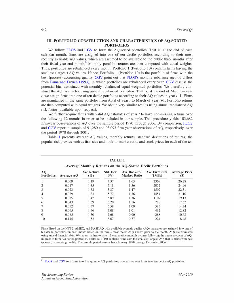
III. PORTFOLIO CONSTRUCTION AND CHARACTERISTICS OF AQ-SORTEDPORTFOLIOS

We follow FLOS and CGV to form the AQ-sorted portfolios. That is, at the end of eachcalendar month, firms are assigned into one of ten decile portfolios according to their mostrecently available AQ values, which are assumed to be available to the public three months aftertheir fiscal year-end month.8 Monthly portfolio returns are then computed with equal weights.Thus, portfolios are rebalanced every month. Portfolio 1 �Portfolio 10� contains firms having thesmallest �largest� AQ values. Hence, Portfolio 1 �Portfolio 10� is the portfolio of firms with thebest �poorest� accounting quality. CGV point out that FLOS’s monthly rebalance method differsfrom Fama and French �1993�, in which portfolios are rebalanced every year. CGV discuss thepotential bias associated with monthly rebalanced equal weighted portfolios. We therefore con-struct the AQ risk factor using annual rebalanced portfolios. That is, at the end of March in yeart, we assign firms into one of ten decile portfolios according to their AQ values in year t−1. Firmsare maintained in the same portfolio from April of year t to March of year t+1. Portfolio returnsare then computed with equal weights. We obtain very similar results using annual rebalanced AQrisk factor �available upon request�.

We further require firms with valid AQ estimates of year t to have non-missing returns overthe following 12 months in order to be included in our sample. This procedure yields 103,682firm-year observations of AQ over the sample period 1970 through 2006. By comparison, FLOSand CGV report a sample of 91,280 and 93,093 firm-year observations of AQ, respectively, overthe period 1970 through 2001.

Table 1 presents average AQ values, monthly returns, standard deviations of returns, thepopular risk proxies such as firm size and book-to-market ratio, and stock prices for each of the ten

8 FLOS and CGV sort firms into five quintile AQ portfolios, whereas we sort firms into ten decile AQ portfolios.

TABLE 1

Average Monthly Returns on the AQ-Sorted Decile Portfolios

AQPortfolios Average AQ

Ave Return(%)

Std. Dev.(%)

Ave Book-to-Market Ratio

Ave Firm Size($Mils)

Average Price($)

1 0.009 1.19 4.37 1.63 2369 26.282 0.017 1.35 5.11 1.56 2052 24.963 0.023 1.32 5.37 1.47 1592 22.514 0.029 1.33 5.77 1.36 1454 21.105 0.035 1.42 5.89 1.36 1107 19.136 0.043 1.39 6.20 1.16 788 17.527 0.052 1.37 6.58 1.09 583 14.748 0.065 1.46 7.08 1.01 432 12.829 0.085 1.50 7.68 0.90 288 10.6810 0.145 1.52 8.67 0.77 224 8.48

Firms listed on the NYSE, AMEX, and NASDAQ with available accruals quality �AQ� measures are assigned into one often decile portfolios on each month based on the firm’s most recent AQs known prior to the month. AQs are estimatedusing annual financial data. We request a firm to have 12 consecutive monthly returns following the announcement of AQsin order to form AQ-sorted portfolios. Portfolio 1 �10� contains firms with the smallest �largest� AQ, that is, firms with best�poorest� accounting quality. The sample period covers from January 1970 through December 2006.

942 Kim and Qi


decile AQ-sorted portfolios. Average monthly returns increase almost monotonically with themagnitude of the AQ from 1.19 percent �Portfolio 1� to 1.52 percent �Portfolio 10�. Portfolios withpoor AQ also have a greater standard deviation of returns. Poor AQ firms have smaller firm size,lower book-to-market ratio, and lower stock price. The mean and median of our AQ measure are0.0535 and 0.0372, respectively �not reported�, which are similar to FLOS’s AQ measures. FLOSreport a mean of 0.0442 and a median of 0.0313.

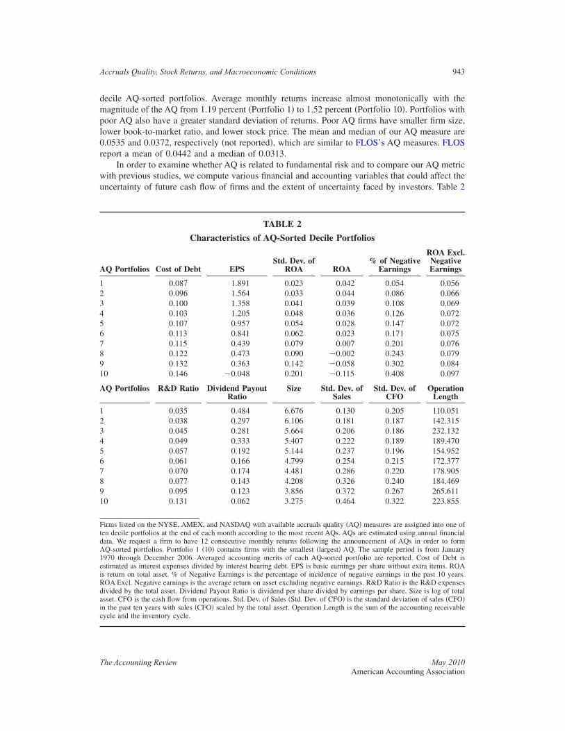
In order to examine whether AQ is related to fundamental risk and to compare our AQ metricwith previous studies, we compute various financial and accounting variables that could affect theuncertainty of future cash flow of firms and the extent of uncertainty faced by investors. Table 2

TABLE 2

Characteristics of AQ-Sorted Decile Portfolios

AQ Portfolios Cost of Debt EPSStd. Dev. of

ROA ROA% of Negative

Earnings

ROA Excl.NegativeEarnings

1 0.087 1.891 0.023 0.042 0.054 0.0562 0.096 1.564 0.033 0.044 0.086 0.0663 0.100 1.358 0.041 0.039 0.108 0.0694 0.103 1.205 0.048 0.036 0.126 0.0725 0.107 0.957 0.054 0.028 0.147 0.0726 0.113 0.841 0.062 0.023 0.171 0.0757 0.115 0.439 0.079 0.007 0.201 0.0768 0.122 0.473 0.090 �0.002 0.243 0.0799 0.132 0.363 0.142 �0.058 0.302 0.08410 0.146 �0.048 0.201 �0.115 0.408 0.097

AQ Portfolios R&D Ratio Dividend PayoutRatio

Size Std. Dev. ofSales

Std. Dev. ofCFO

OperationLength

1 0.035 0.484 6.676 0.130 0.205 110.0512 0.038 0.297 6.106 0.181 0.187 142.3153 0.045 0.281 5.664 0.206 0.186 232.1324 0.049 0.333 5.407 0.222 0.189 189.4705 0.057 0.192 5.144 0.237 0.196 154.9526 0.061 0.166 4.799 0.254 0.215 172.3777 0.070 0.174 4.481 0.286 0.220 178.9058 0.077 0.143 4.208 0.326 0.240 184.4699 0.095 0.123 3.856 0.372 0.267 265.61110 0.131 0.062 3.275 0.464 0.322 223.855

Firms listed on the NYSE, AMEX, and NASDAQ with available accruals quality �AQ� measures are assigned into one often decile portfolios at the end of each month according to the most recent AQs. AQs are estimated using annual financialdata. We request a firm to have 12 consecutive monthly returns following the announcement of AQs in order to formAQ-sorted portfolios. Portfolio 1 �10� contains firms with the smallest �largest� AQ. The sample period is from January1970 through December 2006. Averaged accounting merits of each AQ-sorted portfolio are reported. Cost of Debt isestimated as interest expenses divided by interest bearing debt. EPS is basic earnings per share without extra items. ROAis return on total asset. % of Negative Earnings is the percentage of incidence of negative earnings in the past 10 years.ROA Excl. Negative earnings is the average return on asset excluding negative earnings. R&D Ratio is the R&D expensesdivided by the total asset. Dividend Payout Ratio is dividend per share divided by earnings per share. Size is log of totalasset. CFO is the cash flow from operations. Std. Dev. of Sales �Std. Dev. of CFO� is the standard deviation of sales �CFO�in the past ten years with sales �CFO� scaled by the total asset. Operation Length is the sum of the accounting receivablecycle and the inventory cycle.



presents financial and accounting characteristics of AQ-sorted decile portfolios. Some of thesevariables proxy firm’s business fundamentals and operating environments and are used to estimatethe innate portion of AQ. Consistent with FLOS and Bharath et al. �2008�, we find that poorer AQfirms are associated with higher cost of debt.9 The best AQ firms �Portfolio 1� have a mean cost ofdebt of 8.7 percent, while the poorest AQ firms �Portfolio 10� have a mean cost of debt of 14.6percent. The increase in the cost of debt is monotonic across AQ portfolios, with magnitudessimilar to the 8.98 percent and 10.77 percent reported by FLOS for their best and worst AQquintile portfolios, respectively.

For profitability measures, we consider earnings per share �EPS�, returns on total assets�ROA�, the incidence of negative earnings in the past 10 years and ROA excluding negativeearnings. As shown in Table 2, AQ is negatively related to EPS and ROA. For example, Portfolio1 has an ROA of 4.2 percent, while Portfolio 10 has an ROA of �11.5 percent. Moreover, thepercentage of negative earnings over the past 10 years increases with AQ. That is, the probabilityof negative earnings for firms in the poorest AQ portfolio is 40.8 percent, while the same prob-ability for firms in the best AQ portfolio is only 5.4 percent. When positive earnings are computedalone, firms in the poorest AQ portfolio have the highest earnings. This is consistent with thefinding that poorer AQ portfolios are associated with higher standard deviation of ROA.

As for growth opportunity measures, we consider the R&D ratio �R&D expenses divided bytotal assets� and dividend payout ratio. We find that high AQ firms tend to have a high R&D ratioand a high retention ratio �i.e., low dividend payout ratio�. This is consistent with the findingpresented in Table 1 that poorer AQ firms have lower book-to-market ratios, suggesting that firmswith poorer AQ tend to be growth firms. In addition, we find that firms with poor AQ have greatervariability in sales and cash flow from operations and longer operation cycles.10 Overall, Table 2provides preliminary evidence that AQ is related to firm operating environment and businessnature.

IV. TESTS OF WHETHER ACCRUALS QUALITY IS PRICED IN STOCK RETURNSIn this section, we first construct the AQ risk factor using a method similar to FLOS and

CGV. We then employ the Fama and MacBeth �1973� two-stage cross-sectional regression methodto examine whether AQ is a priced risk factor.

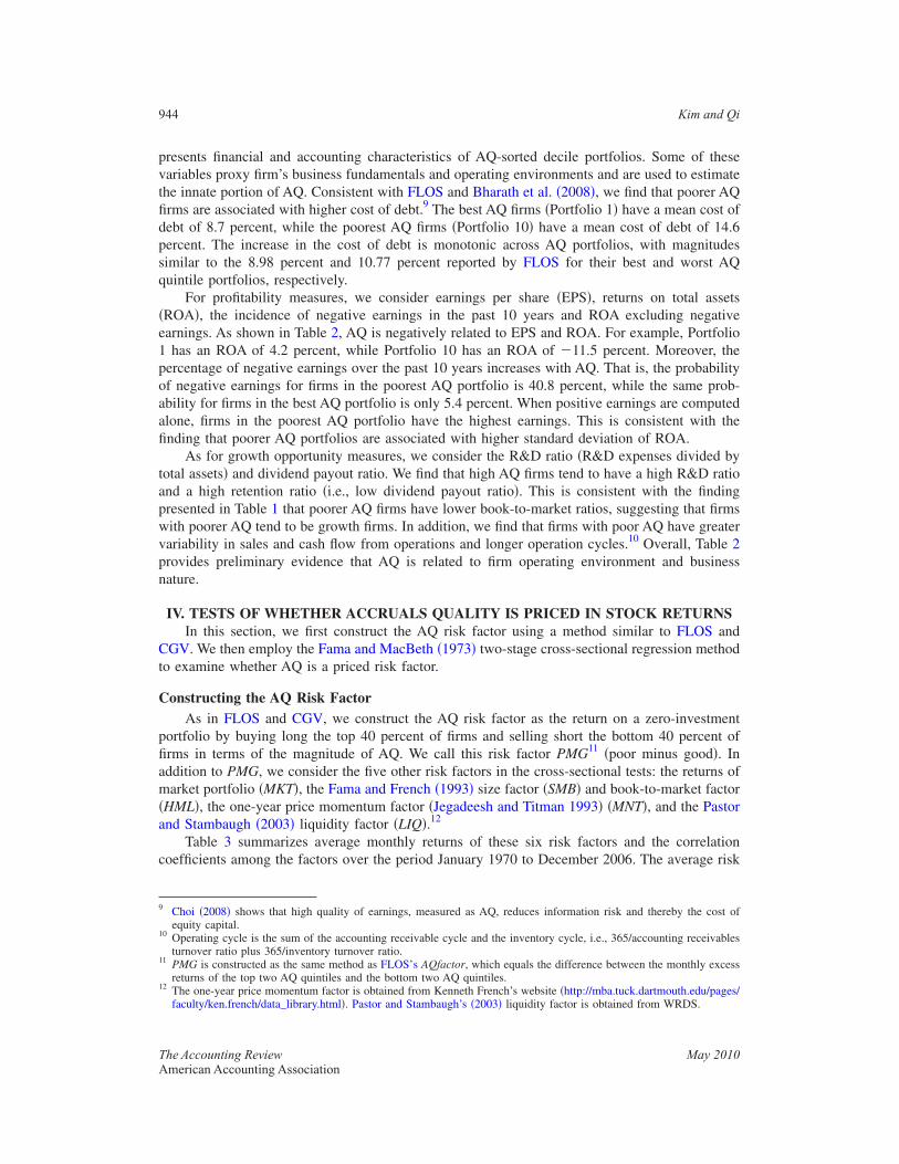
Constructing the AQ Risk FactorAs in FLOS and CGV, we construct the AQ risk factor as the return on a zero-investment

portfolio by buying long the top 40 percent of firms and selling short the bottom 40 percent offirms in terms of the magnitude of AQ. We call this risk factor PMG11 �poor minus good�. Inaddition to PMG, we consider the five other risk factors in the cross-sectional tests: the returns ofmarket portfolio �MKT�, the Fama and French �1993� size factor �SMB� and book-to-market factor�HML�, the one-year price momentum factor �Jegadeesh and Titman 1993� �MNT�, and the Pastorand Stambaugh �2003� liquidity factor �LIQ�.12

Table 3 summarizes average monthly returns of these six risk factors and the correlationcoefficients among the factors over the period January 1970 to December 2006. The average risk

9 Choi �2008� shows that high quality of earnings, measured as AQ, reduces information risk and thereby the cost ofequity capital.

10 Operating cycle is the sum of the accounting receivable cycle and the inventory cycle, i.e., 365/accounting receivablesturnover ratio plus 365/inventory turnover ratio.

11 PMG is constructed as the same method as FLOS’s AQfactor, which equals the difference between the monthly excessreturns of the top two AQ quintiles and the bottom two AQ quintiles.

12 The one-year price momentum factor is obtained from Kenneth French’s website �http://mba.tuck.dartmouth.edu/pages/faculty/ken.french/data_library.html�. Pastor and Stambaugh’s �2003� liquidity factor is obtained from WRDS.

944 Kim and Qi


http://mba.tuck.dartmouth.edu/pages/faculty/ken.french/data_library.html

http://mba.tuck.dartmouth.edu/pages/faculty/ken.french/data_library.html

premia on MKTRFT, SMB, HML, PMG, MNT, and LIQ are 0.494 percent, 0.171 percent, 0.502percent, 0.166 percent, and 0.805, and �0.081 percent per month, respectively. The 0.704 corre-lation coefficient between SMB and PMG is particularly large. This is because smaller firms tendto have poorer AQ than larger firms. PMG correlates negatively with HML.

Models for Cross-Sectional Regression (CSR) TestsWe use the Fama and MacBeth �1973� two-stage cross-sectional regression to examine

whether PMG is a priced risk factor.13 In the first stage, we estimate betas using time-seriesregressions. In the second stage, we use the betas estimated in the first stage as explanatoryvariables in the cross-sectional regressions �CSR�. The CSR model to be estimated at time t is:

Rit − Rft = �0t + �1t�̂i,MKT + �2t�̂i,SMB + �3t�̂i,HML + �4t�̂i,MNT + �5t�̂i,LIQ + �6t�̂i,PMG + �it, �2�

where �̂i is asset i’s beta for a particular risk factor estimated from the first-stage multiple time-series regression model. Rit is asset i’s return at time t, and Rft is the one-month Treasury billreturn at time t. MKT is the CRSP value-weighted market return. The time-series average �̄̂k of theCSR coefficient �� estimates of Equation �2� is regarded as the risk premium estimate of thecorresponding risk factor.

In tests of pricing ability for a given risk factor, especially information risk factors such asPMG, it is necessary to control for low-priced returns because the relation between information

13 Before conducting the main cross-sectional regression tests, we have estimated time-series regressions of returns of tendecile size-sorted portfolios on PMG and the other risk factors considered in order to preliminarily examine whetherthere is a cross-sectional relation between average returns and the factor loadings �or betas� on the risk factors. We findthat the factor loading on PMG has a stronger cross-sectional relation with average returns than any other factorloadings. Furthermore, the PMG has a stronger intertemporal explanatory power for returns on size-sorted portfoliosthan any other risk factors considered. The results are available upon request.

TABLE 3

Basic Statistics of the Risk Factors

MKTRFT SMB HML PMG MNT LIQ

Average Return �%� 0.494 0.171 0.502 0.166 0.805 �0.081Correlation Coefficients

MKTRFT 1.000SMB 0.282 1.000HML �0.443 �0.305 1.000PMG 0.362 0.704 �0.448 1.000MNT �0.084 �0.007 �0.103 �0.078 1.000LIQ 0.373 0.151 �0.122 0.094 �0.039 1.000

The sample period covers from January 1970 through December 2006.

Variable Definitions

MKTRFT � CRSP value-weighted market return in excess of the risk-free return;SMB and HML � Fama and French’s �1993� risk factors, which are related to firm size and book-to-market, respectively;

PMG � returns on the zero-investment portfolio by selling the best 40 percent AQ firms and buying thepoorest 40 percent AQ firms, and it is the risk factor related to accruals quality;

MNT � risk factor related to stock price momentum �obtained from Kenneth French’s website�; andLIQ � Pastor and Stambaugh’s �2003� liquidity risk factor.



risk and returns tends to be severely distorted in low-priced stocks due to the bias in measuredrealized returns. Realized returns may be biased due to noise trading, sentiment trading, andmarket-microstructure induced effects. This bias is notoriously more pronounced in low-pricedstocks �Bhardwaj and Brooks 1992; Ball et al. 1995; Conrad and Kaul 1993; Baker and Wurgler�2006�. Another possible reason is illiquidity. A stock with poor liquidity is often traded inactively.Hence, newly released information would be hardly impounded into stock prices due to the lack offrequent trading. Since illiquidity is especially severe in low-priced stocks, the pricing effect ofinformation risk on stock returns would be difficult to detect in low-priced stocks.

The literature shows that the biased returns of low-priced stocks tend to spuriously exaggeratemarket anomalies. For example, Bhardwaj and Brooks �1992� show that the January anomaly isdriven mainly by low-priced stocks, and Conrad and Kaul �1993� and Ball et al. �1995� argue thatprofits of contrarian strategies are largely attributable to low-priced stocks. Accordingly, the ex-clusion of low-priced stocks in asset pricing tests is not unusual in the literature. Jegadeesh andTitman �2001� exclude stocks with prices below $5 in evaluating explanations of momentumstrategies. Bali et al. �2005� also screen stocks with prices less than $5 in studying idiosyncraticvolatility risk. We control for low-price returns by including an indicator variable in Equation �2�that equals 1 if the return is calculated with the adjacent prices less than $5, and 0 otherwise, ratherthan excluding low-priced returns in the test assets.14 We also provide a robustness check byexcluding the low-priced returns, obtaining similar results.

Individual Stocks versus Portfolios as Test AssetsThere is a trade-off between using individual stocks and using portfolios in the two-stage asset

pricing tests with respect to the measurement error of the beta in the first stage and test power inthe second stage. Tests using portfolios reduce the errors-in-variables �EIV� bias caused by the useof estimated betas instead of true betas, but have weaker test power in examining the explanatorypower of betas for the cross-sectional variation of average returns. On the other hand, tests usingindividual stocks have a stronger testing power, but lead to a greater EIV bias �Shanken 1992; Kim1995, 1997�. Our main concern is, however, on the sensitivity of the test results to the portfolioformation method and data-snooping biases �Lo and MacKinlay 1990�. In particular, when port-folios are used as test assets, we face a more serious problem than the EIV bias or the test powerissues; the results are quite sensitive to how test portfolios are constructed. Moreover, the issue ofbeta measurement error in the first stage could be somewhat resolved, since a relatively longtime-series of return observations are available to estimate betas and thus the beta measurementerror can be reduced. For these reasons, we use individual stocks rather than portfolios for ourtests. In the Appendix �Table A1�, we report estimation results using portfolios similar to CGV’s.

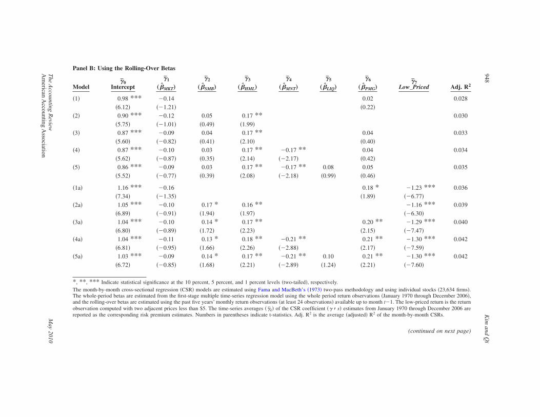
Empirical Results of Cross-Sectional Regression (CSR) TestsTable 4 shows estimation results from month-by-month OLS cross-sectional regressions over

the period January 1970 through December 2006 �444 months� using 23,634 individual firms.Panel A of Table 4 presents CSR results when betas are estimated using whole-period returnobservations. The upper part of Panel A of Table 4, labeled as models �1�–�5�, provides CSRestimation results without controlling for low-priced returns. These results are very similar toCGV �Table 4, Panel D� in terms of the magnitude and statistical significance of estimates. Forexample, when the Fama and French’s �1993; hereafter FF� three factors are included, CGV reportthat the estimated coefficients on MKT, SMB, and HML betas are 0.50 �t � 1.99; p � 0.05 in

14 The benchmark of $5 as low price was used in 1992 by the NYSE when it reduced the minimum tick size to sixteenthsfor stocks under $5.

946 Kim and Qi


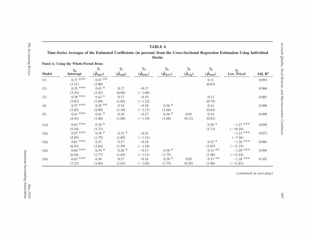
TABLE 4

Time-Series Averages of the Estimated Coefficients (in percent) from the Cross-Sectional Regression Estimation Using IndividualStocks

Panel A: Using the Whole-Period Betas

Model�̄0

Intercept

�̄1

„�̂MKT…

�̄2

„�̂SMB…

�̄3

„�̂HML…

�̄4

„�̂MNT…

�̄5

„�̂LIQ…

�̄6

„�̂PMG…�̄7

Low_Priced Adj. R2

�1� 0.37 *** 0.47 ** 0.11 0.054�3.11� �2.06� �0.63�

�2� 0.35 *** 0.43 * 0.17 �0.17 0.066�3.35� �1.92� �0.96� ��1.08�

�3� 0.38 *** 0.43 * 0.17 �0.19 0.13 0.081�3.83� �1.89� �1.02� ��1.22� �0.75�

�4� 0.37 *** 0.45 ** 0.18 �0.18 0.36 * 0.14 0.090�3.85� �2.00� �1.10� ��1.17� �1.66� �0.83�

�5� 0.41 *** 0.41 * 0.18 �0.17 0.36 * 0.03 0.14 0.099�4.43� �1.86� �1.08� ��1.10� �1.66� �0.12� �0.82�

�1a� 0.62 *** 0.39 * 0.28 * �1.27 *** 0.058�5.54� �1.73� �1.71� ��10.10�

�2a� 0.57 *** 0.39 * 0.32 * �0.21 �1.21 *** 0.073�5.85� �1.75� �1.89� ��1.31� ��7.46�

�3a� 0.61 *** 0.37 0.27 �0.18 0.32 * �1.26 *** 0.084�6.43� �1.64� �1.59� ��1.19� �1.85� ��11.35�

�4a� 0.60 *** 0.39 * 0.28 * �0.17 0.38 * 0.33 ** �1.29 *** 0.094�6.56� �1.77� �1.65� ��1.11� �1.75� �1.96� ��11.64�

�5a� 0.63 *** 0.36 0.27 �0.16 0.38 * 0.05 0.33 ** �1.28 *** 0.103�7.23� �1.64� �1.63� ��1.05� �1.75� �0.20� �1.96� ��11.81�

(continued on next page)

Accruals

Quality,Stock

Returns,and

Macroeconom

icC

onditions947

The

Accounting

Review

May

2010A

merican

Accounting

Association

Panel B: Using the Rolling-Over Betas

Model�̄0

Intercept

�̄1

„�̂MKT…

�̄2

„�̂SMB…

�̄3

„�̂HML…

�̄4

„�̂MNT…

�̄5

„�̂LIQ…

�̄6

„�̂PMG…�̄7

Low_Priced Adj. R2

�1� 0.98 *** �0.14 0.02 0.028

�6.12� ��1.21� �0.22��2� 0.90 *** �0.12 0.05 0.17 ** 0.030

�5.75� ��1.01� �0.49� �1.99��3� 0.87 *** �0.09 0.04 0.17 ** 0.04 0.033

�5.60� ��0.82� �0.41� �2.10� �0.40��4� 0.87 *** �0.10 0.03 0.17 ** �0.17 ** 0.04 0.034

�5.62� ��0.87� �0.35� �2.14� ��2.17� �0.42��5� 0.86 *** �0.09 0.03 0.17 ** �0.17 ** 0.08 0.05 0.035

�5.52� ��0.77� �0.39� �2.08� ��2.18� �0.99� �0.46�

�1a� 1.16 *** �0.16 0.18 * �1.23 *** 0.036

�7.34� ��1.35� �1.89� ��6.77��2a� 1.05 *** �0.10 0.17 * 0.16 ** �1.16 *** 0.039

�6.89� ��0.91� �1.94� �1.97� ��6.30��3a� 1.04 *** �0.10 0.14 * 0.17 ** 0.20 ** �1.29 *** 0.040

�6.80� ��0.89� �1.72� �2.23� �2.15� ��7.47��4a� 1.04 *** �0.11 0.13 * 0.18 ** �0.21 ** 0.21 ** �1.30 *** 0.042

�6.81� ��0.95� �1.66� �2.26� ��2.88� �2.17� ��7.59��5a� 1.03 *** �0.09 0.14 * 0.17 ** �0.21 ** 0.10 0.21 ** �1.30 *** 0.042

�6.72� ��0.85� �1.68� �2.21� ��2.89� �1.24� �2.21� ��7.60�

*, **, *** Indicate statistical significance at the 10 percent, 5 percent, and 1 percent levels �two-tailed�, respectively.The month-by-month cross-sectional regression �CSR� models are estimated using Fama and MacBeth’s �1973� two-pass methodology and using individual stocks �23,634 firms�.The whole-period betas are estimated from the first-stage multiple time-series regression model using the whole period return observations �January 1970 through December 2006�,and the rolling-over betas are estimated using the past five years’ monthly return observations �at least 24 observations� available up to month t�1. The low-priced return is the returnobservation computed with two adjacent prices less than $5. The time-series averages ��̄k� of the CSR coefficient �� s� estimates from January 1970 through December 2006 arereported as the corresponding risk premium estimates. Numbers in parentheses indicate t-statistics. Adj. R2 is the average �adjusted� R2 of the month-by-month CSRs.


948K

imand

Qi

The

Accounting

Review

May

2010A

merican

Accounting

Association


MKT � CRSP value-weighted market returns;SMB and HML � Fama and MacBeth’s �1973� risk factors, which are related to firm size and book-to-market, respectively;

PMG � risk factor related to accruals quality;MNT � risk factor related to stock price momentum;LIQ � Pastor and Stambaugh’s �2003� liquidity risk factor; and

Low_Priced � indicator variable equal to 1 for low-priced returns, and 0 otherwise.

Accruals

Quality,Stock

Returns,and

Macroeconom

icC

onditions949

The

Accounting

Review

May

2010A

merican

Accounting

Association

two-tailed test�, 0.20 �t � 1.05; p � 0.29�, and �0.21 �t � �1.20; p � 0.23�, respectively. Wereport the coefficients as 0.43 �t � 1.92; p � 0.1�, 0.17 �t � 0.96; p � 0.34�, and �0.17 �t ��1.08; p � 0.28�, respectively. When the AQ risk factor �PMG� is added to the FF three-factormodel, CGV report that the coefficient on PMG betas �i.e., �PMC� is 0.25 �t � 0.63; p � 0.53�while we report it as 0.13 �t � 0.75; p � 0.45�.

In fact, the results in the upper part of Table 4, Panel A confirm CGV’s results that the AQbeta is insignificant in any model specification in explaining average stock returns. That is, withoutcontrolling for low-priced returns, the gamma estimates on �PMC are 0.11 percent �t � 0.63; p �0.53�, 0.13 percent �t � 0.75; p � 0.45�, 0.14 percent �t � 0.83; p � 0.41�, and 0.14 percent �t �0.82; p � 0.41�, respectively, for the following four model specifications; �1� market beta plus AQbeta, �2� FF three-factor betas plus AQ beta, �3� FF three-factor betas plus the momentum beta andAQ beta, and �4� FF’s three-factor betas plus the momentum beta, liquidity beta, and AQ beta. Wealso repeat the CSR tests using the same set of test portfolios as in CGV and obtain results similarto CGV. These CSR results using portfolios are reported in the Appendix.

Controlling for low-priced returns, however, the economic and statistical significance of theAQ beta changes substantially. The bottom part of Panel A of Table 4, labeled as models �1a�–�5a�,reports CSR estimation results after controlling for low-priced returns. We find that �PMC ispositively significant in all models considered. For example, the gamma estimates on �PMC � �̂̄6� inthe above four model specifications are 0.28 percent �t � 1.71; p � 0.1�, 0.32 percent �t � 1.85;p � 0.1�, 0.33 percent �t � 1.96; p � 0.05�, and 0.33 percent �t � 1.96; p � 0.05�. We also findthat the significance of the gamma estimates on the other betas and their statistical significanceremain nearly unchanged, even after controlling for low-priced returns. These findings indicatethat the explanatory power of information risk, as proxied by earnings quality, for stock returns isparticularly sensitive to low-priced returns. The estimated coefficients on the indicator variable�Low_Priced� are significantly negative in all models.

Panel B of Table 4 reports CSR results using five-year rolling betas that could update the morerecent risk information.15 The overall results are similar to the case with whole-period betas. Thatis, when low-priced returns are not controlled, the gamma estimates on the AQ beta are alsoinsignificant. After controlling for low-priced returns, however, the gamma estimates on the AQbeta become strongly significant. Regardless of whether we use whole-period or five-year rollingbetas, the significance of the gamma estimates on AQ beta changes more drastically than thegamma estimates on any other betas considered, after controlling for low-priced returns. Note thatall returns are used in constructing the risk factors and portfolios and in estimating betas for theCSR tests throughout this study.16 Low-priced returns are controlled only in the CSR tests byadding the Low_Priced indicator variable to the CSR models. The results presented here suggestonly that the pricing effect of AQ is not found in low-priced returns; but they do not necessarilyimply that the pricing effect of AQ does not exist in low-priced returns.

As a compromise between the greater test power from using individual stocks and the smallerEIV bias from using portfolios, Fama and French �1992� introduced the assigned beta approach. Inthis approach, portfolios are constructed, post-ranking betas are estimated using whole-periodportfolio returns, and the estimated post-ranking portfolio betas are then assigned to individualstocks in the portfolio. This approach mitigates the estimation errors of betas in the first stagetime-series regressions by using portfolios, and then employs individual stocks in the second stagecross-sectional regression tests to increase test power.

15 Betas are estimated by using the most recently available five-year �at least 24 months� monthly return observations.16 The reason that all returns are used in constructing the risk factors including PMG is that a risk factor should be a

well-diversified portfolio in the APT context in which as many assets as possible are included �Ross 1976�.

950 Kim and Qi


Table 5 reports CSR estimation results when individual stock returns are regressed on theassigned betas. In order to obtain the post-ranking portfolio betas, we construct four sets of equallyweighted portfolios: 100 size portfolios, 100 AQ portfolios, 100 size-BM portfolios, and 64 size-BM-AQ portfolios.17 When the assigned betas are obtained from 100 size portfolios, the AQ betais strongly positively significant, no matter whether low-priced returns are controlled or not con-trolled. Even without controlling for low-priced returns, the gamma estimates on the AQ betas �inPanel A� are 1.21 percent �t � 5.54; p � 0.01 in a two-tailed test�, 1.29 percent �t � 5.65; p �0.01�, 1.28 percent �t � 5.63; p � 0.01�, and 1.17 percent �t � 5.16; p � 0.01�, respectively, in theabove-mentioned four model specifications �i.e., �1� market beta AQ beta, �2� FF three-factorbetas AQ beta, �3� FF three-factor betas momentum beta AQ beta, and �4� FF three-factorbetas momentum beta liquidity beta AQ beta�. Controlling for low-priced returns, theexplanatory power of AQ beta for average returns is also stronger. When assigned betas areobtained from 64 size-BM-AQ portfolios, the AQ beta is also strongly positively significant, evenwithout controlling for low-priced returns. When assigned betas are obtained from the other sets ofportfolios �100 AQ portfolios or 100 size-BM portfolios�, the gamma estimates on the AQ beta areinsignificant without controlling for low-priced returns, but strongly positively significant whencontrolling for low-priced returns. Similar to the previous results in Table 4, we also find that theeconomic and statistical significance of the gamma estimates on AQ beta changes substantiallyafter controlling for low-priced returns. However, the economic and statistical significance of theother risk factors remain relatively unchanged even after controlling for low-priced returns. Wealso construct the four sets of portfolios with value weights to obtain the assigned portfolio betas.The CSR results are very similar �available upon request�. In sum, we conclude that CGV’s resultsthat AQ is not significantly priced are driven mostly by low-priced returns.

We report in the Appendix the CSR test results using portfolios with and without controllingfor low-priced returns. These results are comparable with CGV, since the test portfolios �25size-BM portfolios, 100 AQ portfolios, and 64 size-BM-AQ portfolios� are the same as those CGVused. We add two sets of test portfolios: 100 size-BM portfolios and 100 size portfolios. Withoutcontrolling for low-priced returns, the results are similar to CGV. That is, the AQ beta is insig-nificant. After controlling for low-priced returns, however, the AQ beta is significant. Note thatlow-priced returns are controlled by excluding low-priced returns in constructing portfolios be-cause the indicator variable, Low_priced, cannot be used in the CSR when using portfolios. Notealso that the construction of AQ risk factor �PMG� uses all returns including low-priced returns.

V. ACCRUALS QUALITY AND MACROECONOMIC FUNDAMENTALSThe CSR tests in the previous section show that AQ is significantly priced after controlling for

low-priced returns and in many ways is as strong as, or stronger than, the other risk factorsconsidered. The apparent strength of AQ, combined with the previous studies’ finding that theinnate portion of AQ, which is linked with firm’s fundamentals and business environment, has thestrongest cost of capital effects, motivate us to further investigate a linkage of AQ with economicfundamentals. In this section, therefore, we examine whether AQ and its pricing effect varysystematically with fundamental risk, as proxied by macroeconomic variables.

This methodology used to examine the linkage between AQ and economic fundamental risk ismotivated by the recent finance literature on empirical asset pricing tests. Specifically, the exis-tence of the robust risk premium of a hedged portfolio such as SMB may not be sufficient to justifythat this hedged portfolio proxies fundamental risk, since the risk premium may arise only from

17 The two way �size-BM� or three way �size-BM-AQ� portfolios are formed by an independent sorting. That is, thebreak-points in each variable are independently determined, and then stocks are sorted according to these break-points.



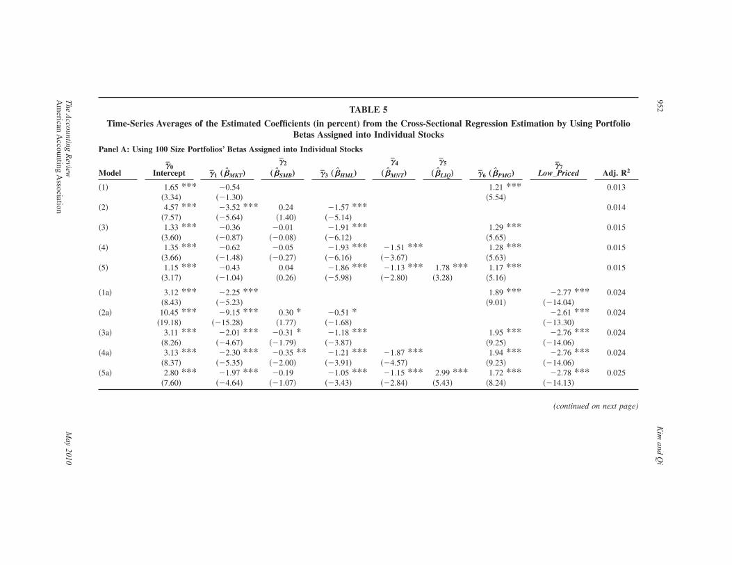
TABLE 5

Time-Series Averages of the Estimated Coefficients (in percent) from the Cross-Sectional Regression Estimation by Using PortfolioBetas Assigned into Individual Stocks

Panel A: Using 100 Size Portfolios’ Betas Assigned into Individual Stocks

Model�̄0

Intercept �̄1 „�̂MKT…

�̄2

„�̂SMB… �̄3 „�̂HML…

�̄4

„�̂MNT…

�̄5

„�̂LIQ… �̄6 „�̂PMG…�̄7

Low_Priced Adj. R2

�1� 1.65 *** �0.54 1.21 *** 0.013�3.34� ��1.30� �5.54�

�2� 4.57 *** �3.52 *** 0.24 �1.57 *** 0.014�7.57� ��5.64� �1.40� ��5.14�

�3� 1.33 *** �0.36 �0.01 �1.91 *** 1.29 *** 0.015�3.60� ��0.87� ��0.08� ��6.12� �5.65�

�4� 1.35 *** �0.62 �0.05 �1.93 *** �1.51 *** 1.28 *** 0.015�3.66� ��1.48� ��0.27� ��6.16� ��3.67� �5.63�

�5� 1.15 *** �0.43 0.04 �1.86 *** �1.13 *** 1.78 *** 1.17 *** 0.015�3.17� ��1.04� �0.26� ��5.98� ��2.80� �3.28� �5.16�

�1a� 3.12 *** �2.25 *** 1.89 *** �2.77 *** 0.024�8.43� ��5.23� �9.01� ��14.04�

�2a� 10.45 *** �9.15 *** 0.30 * �0.51 * �2.61 *** 0.024�19.18� ��15.28� �1.77� ��1.68� ��13.30�

�3a� 3.11 *** �2.01 *** �0.31 * �1.18 *** 1.95 *** �2.76 *** 0.024�8.26� ��4.67� ��1.79� ��3.87� �9.25� ��14.06�

�4a� 3.13 *** �2.30 *** �0.35 ** �1.21 *** �1.87 *** 1.94 *** �2.76 *** 0.024�8.37� ��5.35� ��2.00� ��3.91� ��4.57� �9.23� ��14.06�

�5a� 2.80 *** �1.97 *** �0.19 �1.05 *** �1.15 *** 2.99 *** 1.72 *** �2.78 *** 0.025�7.60� ��4.64� ��1.07� ��3.43� ��2.84� �5.43� �8.24� ��14.13�


952K

imand

Qi

The

Accounting

Review

May

2010A

merican

Accounting

Association

Panel B: Using 100 AQ Portfolios’ Betas Assigned into Individual Stocks

Model�̄0


�̄2

„�̂SMB… �̄3 „�̂HML…

�̄4

„�̂MNT… �̄5 „�̂LIQ…

�̄6

„�̂PMG…�̄7

Low_Priced Adj. R2

�1� 0.37 0.45 0.14 0.010�1.31� �1.15� �0.83�

�2� 0.46 0.37 0.12 �0.16 0.010�1.49� �0.92� �0.55� ��0.56�

�3� 0.43 0.38 0.18 �0.21 0.14 0.011�1.41� �0.95� �0.74� ��0.80� �0.83�

�4� 0.44 0.48 0.13 �0.20 0.59 0.14 0.011�1.42� �1.21� �0.53� ��0.76� �1.50� �0.86�

�5� 0.44 0.48 0.13 �0.20 0.59 0.17 0.15 0.011�1.43� �1.21� �0.53� ��0.75� �1.48� �0.29� �0.86�

�1a� 0.39 0.46 0.39 *** �0.98 *** 0.019�1.38� �1.16� �2.70� ��5.09�

�2a� 0.39 0.46 0.40 ** �0.38 �0.97 *** 0.019�1.27� �1.17� �2.07� ��1.37� ��5.01�

�3a� 0.41 0.45 0.29 �0.26 0.39 *** �0.98 *** 0.020�1.34� �1.13� �1.20� ��0.97� �2.70� ��5.06�

�4a� 0.42 0.58 0.24 �0.25 0.59 0.40 *** �0.98 *** 0.020�1.37� �1.41� �0.98� ��0.93� �1.50� �2.72� ��5.02�

�5a� 0.42 0.58 0.23 �0.26 0.60 0.05 0.40 *** �0.98 *** 0.020�1.36� �1.46� �0.96� ��0.96� �1.53� �0.08� �2.74� ��5.07�

Panel C: Using 100 Size � BM Portfolios’ Betas Assigned into Individual Stocks

Model�̄0


�̄2

„�̂SMB… �̄3 „�̂HML…

�̄4

„�̂MNT… �̄5 „�̂LIQ…

�̄6

„�̂PMG…�̄7

Low_Priced Adj. R2

�1� 2.34 *** �1.66 *** 0.03 0.028�8.33� ��5.04� �0.15�

�2� 2.50 *** �1.89 *** 0.25 0.20 0.029�8.48� ��5.05� �1.17� �1.10�

�3� 2.21 *** �1.54 *** �0.03 0.41 0.02 0.031�8.33� ��4.56� ��0.18� �2.32� �0.11�


Accruals

Quality,Stock

Returns,and

Macroeconom

icC

onditions953

The

Accounting

Review

May

2010A

merican

Accounting

Association

Panel C: Using 100 Size � BM Portfolios’ Betas Assigned into Individual Stocks

Model�̄0


�̄2

„�̂SMB… �̄3 „�̂HML…

�̄4

„�̂MNT… �̄5 „�̂LIQ…

�̄6

„�̂PMG…�̄7

Low_Priced Adj. R2

�4� 1.92 *** �1.15 *** 0.02 0.37 ** 0.96 ** 0.10 0.031�7.68� ��3.47� �0.12� �2.12� �2.34� �0.57�

�5� 1.70 *** �0.98 *** 0.09 0.28 0.87 ** 1.65 *** 0.12 0.031�6.88� ��2.97� �0.53� �1.57� �2.13� �3.10� �0.68�

�1a� 3.56 *** �2.94 *** 0.71 *** �2.38 *** 0.035�13.33� ��9.15� �4.79� ��14.23�

�2a� 4.40 *** �3.83 *** 1.08 *** �0.23 �2.11 *** 0.036�15.73� ��10.71� �6.15� ��1.33� ��12.14�

�3a� 3.30 *** �2.50 *** �0.11 0.68 *** 0.74 *** �2.44 *** 0.038�12.26� ��7.37� ��0.61� �3.86� �5.03� ��14.63�

�4a� 2.71 *** �1.70 *** �0.00 0.60 *** 1.79 *** 0.90 *** �2.45 *** 0.038�10.92� ��5.14� ��0.01� �3.43� �4.44� �5.93� ��14.70�

�5a� 2.22 *** �1.33 *** 0.16 0.38 ** 1.58 *** 4.08 *** 0.96 *** �2.50 *** 0.038�9.13� ��4.04� �0.92� �2.16� �3.98� �7.71� �6.32� ��14.97�

Panel D: Using 64 Size � BM � AQ Portfolios’ Betas Assigned into Individual Stocks

Model�̄0


�̄2

„�̂SMB… �̄3 „�̂HML…

�̄4

„�̂MNT… �̄5 „�̂LIQ…

�̄6

„�̂PMG…�̄7

Low_Priced Adj. R2

�1� 1.10 *** �0.49 ** 0.76 *** 0.012�4.40� ��2.19� �3.43�

�2� 2.52 *** �1.80 *** 0.44 ** �0.41 *** 0.013�4.10� ��3.39� �2.54� ��3.05�

�3� 1.83 *** �0.93 * 0.17 �0.30 ** 0.84 *** 0.018�2.73� ��1.65� �0.84� ��2.44� �3.54�

�4� 1.91 *** �1.05 *** 0.17 �0.34 ** �0.36 0.83 *** 0.019�4.05� ��2.77� �0.74� ��2.38� ��0.31� �3.81�

�5� 2.29 *** �1.41 *** 0.17 �0.28 ** 0.06 �1.58 * 0.75 *** 0.020�4.37� ��2.86� �0.74� ��2.32� �0.05� ��1.81� �3.81�

�1a� 1.48 *** �0.79 *** 1.60 *** �1.59*** 0.020


954K

imand

Qi

The

Accounting

Review

May

2010A

merican

Accounting

Association

Panel D: Using 64 Size � BM � AQ Portfolios’ Betas Assigned into Individual Stocks

Model�̄0


�̄2

„�̂SMB… �̄3 „�̂HML…

�̄4

„�̂MNT… �̄5 „�̂LIQ…

�̄6

„�̂PMG…�̄7

Low_Priced Adj. R2

�4.18� ��3.70� �8.70� ��8.54��2a� 4.62 *** �3.67 *** 0.91 *** �0.97 *** �1.59 *** 0.021

�8.56� ��7.78� �5.86� ��8.78� ��8.63��3a� 3.47 *** �2.17 *** 0.41 ** �0.79 *** 1.69 *** �1.67 *** 0.023

�5.70� ��4.18� �2.19� ��7.71� �7.54� ��8.99��4a� 3.19 *** �1.87 *** 0.46 ** �0.72 *** 0.71 1.72 *** �1.65 *** 0.027

�7.28� ��4.99� �2.14� ��5.53� �0.64� �8.87� ��9.11��5a� 4.17 *** �2.80 *** 0.46 ** �0.55 *** 1.85 ** �3.75 *** 1.52 *** �1.67 *** 0.027

�8.50� ��5.72� �2.19� ��4.92� �1.96� ��4.27� �8.64� ��9.20�

*, **, *** Indicate statistical significance at the 10 percent, 5 percent, and 1 percent levels �two-tailed�, respectively.As in Fama and French �1992�, portfolios are first formed according to a particular value �firm size, book-to-market, and/or AQ� by rebalancing every year, and betas of the portfoliosare computed by using the whole-period returns. The betas of the portfolios are then assigned into individual stocks that were included in the portfolio. The cross-sectional regression�CSR� models of individual stocks’ returns on the individual stock’s assigned betas are estimated month by month. The total number of individual stocks used is 23,634 firms. Thelow-priced return is the return observation computed with two adjacent prices less than $5. The time-series averages ��̄k� of the CSR coefficient �� s� estimates from January 1970through December 2006 are reported as the corresponding risk premium estimates. Numbers in parentheses indicate t-statistics. Adj. R2 is the average �adjusted� R2 of themonth-by-month CSRs.


MKT � CRSP value-weighted market returns;SMB and HML � Fama and French’s �1993� risk factors, which are related to firm size and book-to-market, respectively;

PMG � risk factor related to accruals quality;MNT � risk factor related to stock price momentum;LIQ � Pastor and Stambaugh’s �2003� liquidity risk factor; and

Low_Priced � indicator variable equal to 1 for low-priced returns, and 0 otherwise.

Accruals

Quality,Stock

Returns,and

Macroeconom

icC

onditions955

The

Accounting

Review

May

2010A

merican

Accounting

Association

market mispricing. Examination of whether the risk premium of a proposed risk factor is relatedto “state variables,” as proxied by macroeconomic measures, is a widely used method to determinewhether the risk factor is related to fundamental risk �Chen 1991; Pontiff and Schall 1998; Liewand Vassalou 2000; Chordia and Shivakumar 2002, 2006�. For example, Liew and Vassalou �2000�test whether returns on SMB, HML, and MNT are linked to future gross domestic product �GDP�growth. They find that SMB and HML are proxies of fundamental risk, but MNT is not. Chordiaand Shivakumar �2002� study the relation between momentum profits and a set of macroeconomicvariables arguing that momentum profits are not abnormal profits but rather a risk premiumsourced from the change of fundamental risk. In this study, we follow this line of research to studywhether the risk premium associated with earnings quality varies with macroeconomic conditions.If the AQ-return relationship found in the previous section is induced by the fundamental riskembedded in earnings quality, then we expect that returns of AQ-sorted portfolios vary system-atically with macroeconomic conditions.

Moreover, the literature documents that the portion of earnings quality associated with innatefactors, which stem from the firm’s business model and operating environment, is strongly asso-ciated with the cost of capital, whereas the discretionary portion is much more weakly associatedwith the cost of capital �see Dechow and Dichev 2002; FLOS�. In order to further investigate theAQ-return relation, we decompose the AQ into its innate and discretionary portions and examinethe relation between each of these aspects of AQ and macroeconomic conditions. If the innateportion of AQ is more associated with the cost of capital, then we expect returns of innateAQ-sorted portfolios to vary systematically with macroeconomic shocks.

Decomposing Accruals Quality into Innate and Discretionary ComponentsIn order to decompose total AQ into innate and discretionary portions, we follow FLOS and

Dechow and Dichev �2002�, as follows:

AQj,t = 0 + 1Sizej,t + 2Std�CFO� j,t + 3Std�Sales� j,t + 4OperCyclej,t + 5NegEarnj,t + � j,t,

�3�

where AQj,t is the estimated accruals quality of firm j at year t using Equation �1�; Size is the logof total assets; Std�CFO� is the standard deviation of cash flow from operations in the past 10years; Std�Sales� is the standard deviation of sales in the past ten years; OperCycle is operationcycles calculated as the sum of the accounting receivable cycle and the inventory cycle; andNegEarn is the incidence of negative earnings in the past 10 years. The predicted value from

Equation �3�, AQ̂

j,t, is the innate portion of firm j’s AQ, namely InnAQ. The residual from Equa-tion �3�, �̂ j,t, is the discretionary portion of firm j’s AQ, namely DisAQ.

Since InnAQ measures accruals quality sourced from the firm’s business model and operationenvironment, InnAQ is a proxy of earnings quality attributable to fundamental business risk.DisAQ is a measure of earnings quality stemming from accounting choices, implementation deci-sions, and managerial errors. DisAQ is therefore a proxy of earnings quality arising from mana-gerial discretion. It is important to note that DisAQ is not a pure noise component. Guay et al.�1996� discuss how discretionary accruals can contain up to three subcomponents: performance,opportunism, and pure noise. They find that the performance and opportunism components domi-nate the noise component. FLOS provide evidence that both InnAQ and DisAQ affect cost ofcapital, although InnAQ has a larger impact on cost of capital than does DisAQ.

Accruals Quality and Business CyclesWe begin by characterizing the time-series pattern of returns and AQ �InnAQ and DisAQ�

values of AQ-sorted �InnAQ-sorted and DisAQ-sorted� portfolios over the sample period. Figure 1

956 Kim and Qi


FIGURE 1Returns of Accruals Quality-Sorted Portfolios

Panel A: Returns of AQ-sorted portfolios over business cycles

AQ1 AQ10

Return

-0.5

-0.4

-0.3

-0.2

-0.1

0.0

0.1

0.2

0.3

0.4

0.5

Date

70 72 74 76 78 80 82 84 86 88 90 92 94 96 98 00 02 04 06 08

Panel B: Returns of InnAQ-sorted portfolios over business cycles

InnAQ1 InnAQ10

Return

-0.5

-0.4

-0.3

-0.2

-0.1

0.0

0.1

0.2

0.3

0.4

0.5

Date

70 72 74 76 78 80 82 84 86 88 90 92 94 96 98 00 02 04 06 08

Panel C: Returns of DisAQ-sorted portfolios over business cycles

DisAQ1 DisAQ10

Return

-0.5

-0.4

-0.3

-0.2

-0.1

0.0

0.1

0.2

0.3

0.4

0.5

Date

70 72 74 76 78 80 82 84 86 88 90 92 94 96 98 00 02 04 06 08



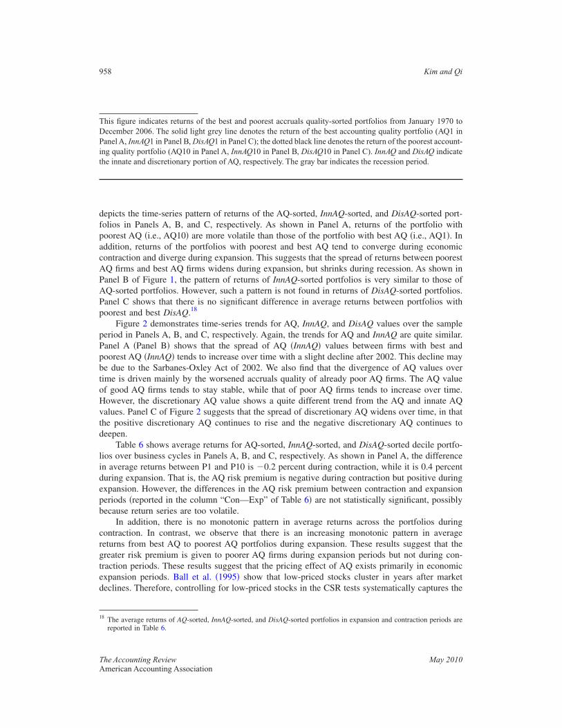
depicts the time-series pattern of returns of the AQ-sorted, InnAQ-sorted, and DisAQ-sorted port-folios in Panels A, B, and C, respectively. As shown in Panel A, returns of the portfolio withpoorest AQ �i.e., AQ10� are more volatile than those of the portfolio with best AQ �i.e., AQ1�. Inaddition, returns of the portfolios with poorest and best AQ tend to converge during economiccontraction and diverge during expansion. This suggests that the spread of returns between poorestAQ firms and best AQ firms widens during expansion, but shrinks during recession. As shown inPanel B of Figure 1, the pattern of returns of InnAQ-sorted portfolios is very similar to those ofAQ-sorted portfolios. However, such a pattern is not found in returns of DisAQ-sorted portfolios.Panel C shows that there is no significant difference in average returns between portfolios withpoorest and best DisAQ.18

Figure 2 demonstrates time-series trends for AQ, InnAQ, and DisAQ values over the sampleperiod in Panels A, B, and C, respectively. Again, the trends for AQ and InnAQ are quite similar.Panel A �Panel B� shows that the spread of AQ �InnAQ� values between firms with best andpoorest AQ �InnAQ� tends to increase over time with a slight decline after 2002. This decline maybe due to the Sarbanes-Oxley Act of 2002. We also find that the divergence of AQ values overtime is driven mainly by the worsened accruals quality of already poor AQ firms. The AQ valueof good AQ firms tends to stay stable, while that of poor AQ firms tends to increase over time.However, the discretionary AQ value shows a quite different trend from the AQ and innate AQvalues. Panel C of Figure 2 suggests that the spread of discretionary AQ widens over time, in thatthe positive discretionary AQ continues to rise and the negative discretionary AQ continues todeepen.

Table 6 shows average returns for AQ-sorted, InnAQ-sorted, and DisAQ-sorted decile portfo-lios over business cycles in Panels A, B, and C, respectively. As shown in Panel A, the differencein average returns between P1 and P10 is �0.2 percent during contraction, while it is 0.4 percentduring expansion. That is, the AQ risk premium is negative during contraction but positive duringexpansion. However, the differences in the AQ risk premium between contraction and expansionperiods �reported in the column “Con—Exp” of Table 6� are not statistically significant, possiblybecause return series are too volatile.

In addition, there is no monotonic pattern in average returns across the portfolios duringcontraction. In contrast, we observe that there is an increasing monotonic pattern in averagereturns from best AQ to poorest AQ portfolios during expansion. These results suggest that thegreater risk premium is given to poorer AQ firms during expansion periods but not during con-traction periods. These results suggest that the pricing effect of AQ exists primarily in economicexpansion periods. Ball et al. �1995� show that low-priced stocks cluster in years after marketdeclines. Therefore, controlling for low-priced stocks in the CSR tests systematically captures the

18 The average returns of AQ-sorted, InnAQ-sorted, and DisAQ-sorted portfolios in expansion and contraction periods arereported in Table 6.

This figure indicates returns of the best and poorest accruals quality-sorted portfolios from January 1970 toDecember 2006. The solid light grey line denotes the return of the best accounting quality portfolio (AQ1 inPanel A, InnAQ1 in Panel B, DisAQ1 in Panel C); the dotted black line denotes the return of the poorest account-ing quality portfolio (AQ10 in Panel A, InnAQ10 in Panel B, DisAQ10 in Panel C). InnAQ and DisAQ indicatethe innate and discretionary portion of AQ, respectively. The gray bar indicates the recession period.

958 Kim and Qi


TABLE 6

Average Returns of Accruals Quality-Sorted Portfolio over Business Cycle

Panel A: Returns of AQ-Sorted Portfolio in Contraction and Expansion Periods

AQ Portfolios

Contraction Expansion Con � Exp

Mean„�C… t-value

Mean„�E… t-value �E − �C

t-testH0: �E = �C

1 0.009 �1.07� 0.013 �6.29�*** 0.004 �0.46�2 0.011 �1.14� 0.014 �5.89�*** 0.003 �0.35�3 0.009 �0.95� 0.014 �5.58�*** 0.005 �0.52�4 0.008 �0.78� 0.014 �5.32�*** 0.006 �0.62�5 0.008 �0.75� 0.015 �5.54�*** 0.007 �0.68�6 0.007 �0.67� 0.015 �5.08�*** 0.008 �0.76�7 0.008 �0.69� 0.015 �4.77�*** 0.007 �0.58�8 0.007 �0.63� 0.016 �4.67�*** 0.008 �0.69�9 0.006 �0.53� 0.017 �4.48�*** 0.010 �0.80�10 0.006 �0.48� 0.017 �3.89�*** 0.010 �0.76�P10 � P1 �0.002 ��0.34� 0.004 �1.28� 0.007 �0.84�

Panel B: Returns of InnAQ-Sorted Portfolio in Contraction and Expansion Periods

InnAQ Portfolios





1 0.009 �1.23� 0.012 �6.29�*** 0.002 �0.31�2 0.009 �1.07� 0.013 �6.04�*** 0.004 �0.45�3 0.011 �1.20� 0.013 �5.68�*** 0.003 �0.28�4 0.009 �0.90� 0.013 �5.27�*** 0.004 �0.40�5 0.008 �0.82� 0.014 �5.52�*** 0.006 �0.61�6 0.008 �0.82� 0.014 �5.26�*** 0.006 �0.56�7 0.005 �0.48� 0.015 �5.17�*** 0.009 �0.82�8 0.006 �0.54� 0.016 �5.15�*** 0.010 �0.84�9 0.007 �0.64� 0.016 �4.58�*** 0.009 �0.73�


Accruals

Quality,Stock

Returns,and

Macroeconom

icC

onditions959

The

Accounting

Review

May

2010A

merican

Accounting

Association

Panel B: Returns of InnAQ-Sorted Portfolio in Contraction and Expansion Periods

InnAQ Portfolios





10 0.008 �0.59� 0.018 �4.33�*** 0.010 �0.72�P10 � P1 �0.001 ��0.14� 0.006 �1.71�* 0.008 �0.72�

Panel C: Returns of DisAQ-Sorted Portfolio in Contraction and Expansion Periods

DisAQ Portfolios





1 0.010 �0.89� 0.016 �5.21�*** 0.006 �0.54�2 0.008 �0.83� 0.016 �5.89�*** 0.008 �0.77�3 0.010 �1.07� 0.015 �6.23�*** 0.005 �0.56�4 0.010 �1.07� 0.014 �6.00�*** 0.005 �0.50�5 0.008 �0.81� 0.014 �5.76�*** 0.006 �0.56�6 0.009 �0.97� 0.013 �5.35�*** 0.004 �0.41�7 0.008 �0.89� 0.014 �5.45�*** 0.005 �0.56�8 0.005 �0.47� 0.014 �5.49�*** 0.009 �0.86�9 0.005 �0.47� 0.013 �4.75�*** 0.008 �0.77�10 0.008 �0.70� 0.015 �4.48�*** 0.007 �0.56�P10 � P1 �0.002 ��0.48� �0.001 ��0.63� 0.001 �0.22�

*, **, *** Indicate statistical significance at the 10 percent, 5 percent, and 1 percent levels �two-tailed�, respectively.This table presents the summary statistics of the returns of AQ-Sorted, InnAQ-Sorted, and DisAQ-Sorted decile portfolios in expansion and contraction periods in Panels A, B, andC, respectively. Con–Exp indicates the difference in the average returns between contraction and expansion periods. The sample period covers January 1970 through December 2006.P10 � P1 is the return from selling Portfolio 1 �best accruals quality� and buying Portfolio 10 �poorest accruals quality�. InnAQ and DisAQ indicate the innate and discretionaryportion of AQ, respectively.

960K

imand

Qi

The

Accounting

Review

May

2010A

merican

Accounting

Association

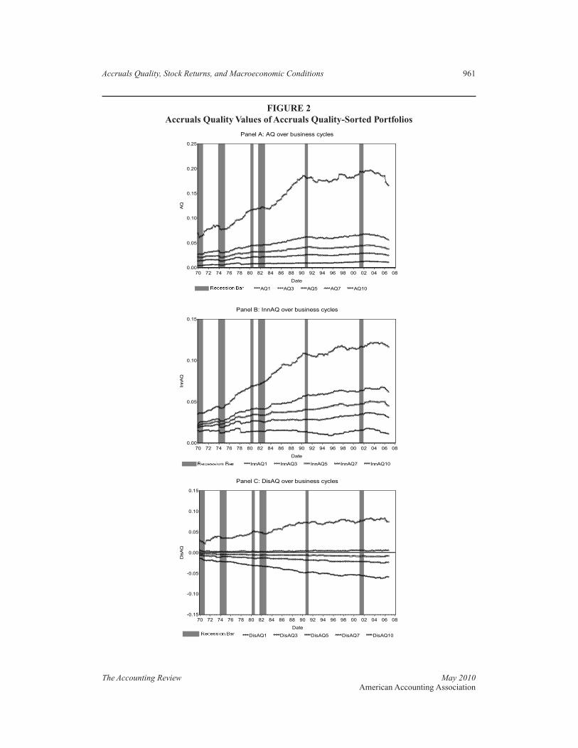
FIGURE 2Accruals Quality Values of Accruals Quality-Sorted Portfolios

Panel A: AQ over business cycles

AQ1 AQ3 AQ5 AQ7 AQ10

AQ

0.00

0.05

0.10

0.15

0.20

0.25

Date

70 72 74 76 78 80 82 84 86 88 90 92 94 96 98 00 02 04 06 08

Panel B: InnAQ over business cycles

InnAQ1 InnAQ3 InnAQ5 InnAQ7 InnAQ10

InnAQ

0.00

0.05

0.10

0.15

Date

70 72 74 76 78 80 82 84 86 88 90 92 94 96 98 00 02 04 06 08

Panel C: DisAQ over business cycles

DisAQ1 DisAQ3 DisAQ5 DisAQ7 DisAQ10

DisAQ

-0.15

-0.10

-0.05

0.00

0.05

0.10

0.15

Date

70 72 74 76 78 80 82 84 86 88 90 92 94 96 98 00 02 04 06 08



recession effect. This can be a reason why the performance of the AQ risk factor changes sub-stantially once low-priced stocks are controlled in the CSR test. This evidence that the AQ pricingeffect is driven mainly during economic expansion periods is also consistent with the notion thatthe AQ risk is related to growth. We provide evidence that AQ is related to growth, as measuredby the book-to-market ratio, R&D expense ratio, and dividend payout ratio in Tables 1 and 2.

Another interesting finding is that when the economy changes from bad state �contraction� togood state �expansion�, returns of firms with poor AQ increase more sharply than returns of firmswith good AQ. For example, the return of P10 increases from 0.6 percent to 1.7 percent from badstate to good state, while the return of P1 increases from 0.9 percent to 1.3 percent.

Panel B of Table 6 provides average returns and innate AQ values for InnAQ-sorted portfoliosover business cycles. The results are very similar to those of AQ-sorted portfolios. The riskpremium of innate AQ is positive in expansion but negative in contraction. Moreover, the riskpremium of innate AQ is even greater than the risk premium of AQ in terms of magnitude andstatistical significance. During expansion periods, for example, the risk premium of innate AQ�P10—P1 in Panel B� is 0.6 percent �t � 1.71; p � 0.1�, and the risk premium of AQ �P10—P1in Panel A� is 0.4 percent �t � 1.28; p � 0.20�. The results using discretionary AQ-sortedportfolios, however, are quite different from those using AQ-sorted and InnAQ-sorted portfolios.Panel C of Table 6 shows that the risk premium of discretionary AQ �P10—P1 in Panel C� is quitesmall and even negative in both contraction and expansion periods. It is �0.2 percent in contrac-tion and �0.1 percent in expansion. No monotonic pattern of average returns across DisAQ-sortedportfolios characterizes either contraction or expansion periods. Overall, these results suggest thatthe innate portion of AQ varies symmetrically with business cycles and affects cost of capital, butthe discretionary portion of AQ does not.

Accruals Quality and Macroeconomic Conditions

In order to further examine whether the AQ risk factor is systematically related to fundamen-tal risk that stems from macroeconomic conditions, we regress the returns of AQ-sorted portfolioson macroeconomic variables. Following the literature, we adopt five macroeconomic variablesrepresenting financial market conditions: �1� the yield on the three-month Treasury Bill �TB�; �2�the return of the market portfolio �MKT�, defined as return of the CRSP value-weighted index; �3�the term spread �TERM�, defined as the difference between the yield on ten-year governmentbonds and the yield on the three-month Treasury Bill; �4� the default spread �DEFAULT�, definedas the difference between the yield on Moody’s BAA rated bonds and the yield on Moody’s AAA

This figure presents the values of AQ, InnAQ, and DisAQ of AQ-, InnAQ-, and DisAQ-sorted portfolios fromJanuary 1970 to December 2006 in Panels A, B, and C, respectively. InnAQ and DisAQ indicate the innate anddiscretionary portion of AQ, respectively. Among ten deciles portfolios, only five portfolios (best, third best,fifth best, seventh best, and poorest accounting quality) are denoted (i.e., AQ1, AQ3, AQ5, AQ7, AQ10 in PanelA; InnAQ1, InnAQ3, InnAQ5, InnAQ7, InnAQ10 in Panel B; DisAQ1, DisAQ3, DisAQ5, DisAQ7, DisAQ10 inPanel C). Solid line denotes the best AQ (InnAQ, DisAQ) portfolio, dotted line denotes the poorest AQ (InnAQ,DisAQ) portfolio, the three broken lines from the bottom to up represent the third best, fifth best, and seventhbest AQ (InnAQ, DisAQ) portfolios, respectively. The gray bar indicates the recession period.

962 Kim and Qi


rated bonds; and �5� the dividend yield on the market �DIV�, defined as the total dividend yield ofthe CRSP value-weighted index.19

Panel A of Table 7 presents estimation results of the time-series regressions of AQ-sortedportfolio returns on these macroeconomic variables. We find that the absolute value of the esti-mated coefficients increases almost monotonically from the best AQ portfolio to the poorest AQportfolio for each of the five financial market variables, consistent with the notion that poor AQfirms are more responsive to changes in financial market conditions. For example, a 1 percentincrease in the market portfolio return is associated with an increase of 0.826 percent return on thebest AQ portfolio �P1�, but an increase of 1.431 percent return on the poorest AQ portfolio�P10�.20 On the other hand, a 1 percent increase in the Treasury bill rate is associated with adecrease of 0.178 percent return on the best AQ portfolio, but a decrease of 1.955 percent returnon the poorest AQ portfolio. That is, when the market interest rate rises, returns of poor AQ firmsfall more severely; when the market return increases, returns of poor AQ firms soar more sharply.

The last row in Table 7, Panel A shows the regression results of the difference in returnsbetween AQ Portfolios 10 and 1 �P10—P1� on the five macroeconomic variables. This differenceis the return on a zero-investment portfolio and can be regarded as the risk premium for bearingAQ risk. The results suggest that the AQ risk premium increases with market return �estimatedcoefficient � 0.605; t � 10.2; p � 0.01�, while it decreases with the Treasury bill rate �estimatedcoefficient � �1.777; t � �1.53; p � 0.13�, the term spread �estimated coefficient � �0.613; t� �5.19; p � 0.01�, and the dividend yield �estimated coefficient � �1.964; t � �1.11; p �0.27�. These results are consistent with our previous findings in Table 6 that the risk premium ofAQ increases with economic expansion.

Panel B of Table 7 reports regression results using InnAQ-sorted decile portfolios. Theseresults are quite similar to those in Panel A. That is, the absolute magnitude of the estimatedcoefficient increases monotonically from the best innate AQ portfolio to the poorest innate AQportfolio for each of the five macroeconomic variables. The risk premium of innate AQ �P10—P1in Panel B� is also positively related to market return but is negatively related to Treasury rate,term spread, and dividend yield.

Panel C of Table 7 reports regression results using DisAQ-sorted portfolios. Here, we observeno monotonic pattern in the estimated coefficients. That is, the estimated coefficients on themacroeconomic variables have no relation with the discretionary portion of AQ. Moreover, therisk premium of discretionary AQ �P10—P1 in Panel C� is not significantly related to any mac-roeconomic variables except for the market return variable. The estimated coefficient on themarket return is 0.161 �t � 6.40; p � 0.01�. Although statically significant, the coefficient value ismuch smaller than in AQ-sorted or InnAQ-sorted portfolios. Note that the estimated coefficients onthe market return are 0.605 �t � 10.2; p � 0.01� and 0.546 �t � 7.43; p � 0.01� in the cases ofAQ-sorted and InnAQ-sorted portfolios, respectively.

Accruals Quality and Future Economic ActivityFinally, we relate AQ to future economic activity. Following Chen �1991�, Liew and Vassalou

�2000�, and Chordia and Shivakumar �2006�, we regress each of the 12-month-ahead macroeco-

19 Pontiff and Schall �1998� and Chordia and Shivakumar �2006� also use Treasury Bill, default premium, term spread, anddividend yield as the state variables of economic conditions. They, however, do not include the market portfolio returnas we do in this study. Excluding the market portfolio return greatly reduces the R2 of the regressions but does notchange our results.

20 The coefficient on MKT is essentially a market beta. Table 7 shows that estimated market betas increase monotonicallyacross the AQ deciles. This is indirect evidence that AQ is positively associated with the cost of equity capital. Theseresults are consistent with the results reported in FLOS �2005, Table 2�.



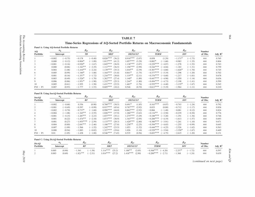
TABLE 7

Time-Series Regressions of AQ-Sorted Portfolio Returns on Macroeconomic FundamentalsPanel A: Using AQ-Sorted Portfolio Returns

AQPortfolio

�p �p1 �p2 �p3 �p4 �p5 Numberof Obs. Adj. R2Intercept TB MKT DEFAULT TERM DIV

1 �0.002 ��0.75� �0.178 ��0.40� 0.826*** �36.2� 0.918*** �3.07� 0.058 �1.29� �1.171* ��1.73� 444 0.7652 0.000 ��0.12� �0.904* ��1.89� 1.012*** �41.2� 1.057*** �3.29� �0.082* ��1.68� �0.983 ��1.35� 444 0.8043 �0.001 ��0.16� �0.920* ��1.67� 1.045*** �36.9� 1.138*** �3.07� �0.229*** ��4.07� �1.278 ��1.52� 444 0.7634 0.000 �0.06� �1.342** ��2.25� 1.112*** �36.5� 1.196*** �2.99� �0.244*** ��4.04� �1.182 ��1.31� 444 0.7595 0.004 �1.08� �1.410** ��2.24� 1.139*** �35.3� 1.010** �2.39� �0.307*** ��4.80� �1.626* ��1.70� 444 0.7456 0.005 �0.99� �1.340* ��1.88� 1.164*** �31.8� 0.841* �1.75� �0.377*** ��5.19� �1.298 ��1.20� 444 0.7027 0.001 �0.16� �1.357* ��1.72� 1.216*** �30.0� 1.119** �2.11� �0.376*** ��4.68� �1.217 ��1.01� 444 0.6788 0.003 �0.49� �1.526* ��1.70� 1.262*** �27.4� 1.140* �1.89� �0.447*** ��4.90� �1.550 ��1.14� 444 0.6369 0.006 �0.86� �1.951* ��1.90� 1.332*** �25.3� 1.244* �1.80� �0.494*** ��4.73� �2.198 ��1.41� 444 0.59910 0.005 �0.61� �1.955 ��1.58� 1.431*** �22.5� 1.463* �1.76� �0.555*** ��4.40� �3.135* ��1.67� 444 0.542P10 � P1 0.007 �0.93� �1.777 ��1.53� 0.605*** �10.2� 0.546 �0.70� �0.613*** ��5.19� �1.964 ��1.11� 444 0.210

Panel B: Using InnAQ-Sorted Portfolio Returns

InnAQPortfolio

�p �p1 �p2 �p3 �p4 �p5 Numberof Obs. Adj. R2Intercept RF MKT DEFAULT TERM DIV

1 �0.002 ��0.68� 0.356 �0.90� 0.780*** �38.5� 0.491* �1.85� 0.163*** �4.07� �0.743 ��1.24� 444 0.7922 �0.001 ��0.49� �0.397 ��0.99� 0.937*** �45.6� 0.787*** �2.92� 0.033 �0.80� �0.712 ��1.17� 444 0.8363 �0.002 ��0.70� �0.737* ��1.68� 0.990*** �44.0� 0.862*** �2.92� �0.066 ��1.48� �0.081 ��0.12� 444 0.8244 �0.004 ��1.08� �1.345** ��2.55� 1.026*** �37.9� 1.286*** �3.63� �0.134** ��2.50� �0.239 ��0.30� 444 0.7765 �0.001 ��0.15� �1.287** ��2.23� 1.037*** �35.1� 1.275*** �3.29� �0.188*** ��3.20� �1.191 ��1.36� 444 0.7466 0.001 �0.22� �1.474** ��2.18� 1.073*** �30.9� 1.343*** �2.95� �0.288*** ��4.19� �1.613 ��1.57� 444 0.6937 0.001 �0.27� �1.955*** ��2.59� 1.133*** �29.3� 1.420*** �2.80� �0.300*** ��3.91� �1.261 ��1.10� 444 0.6718 0.004 �0.80� �2.047** ��2.46� 1.186*** �27.8� 1.258** �2.25� �0.394*** ��4.65� �1.255 ��0.99� 444 0.6459 0.007 �1.09� �1.566 ��1.52� 1.242*** �23.5� 1.053 �1.52� �0.444*** ��4.25� �2.526 ��1.62� 444 0.56310 0.008 �0.94� �1.083 ��0.82� 1.327*** �19.6� 1.026 �1.16� �0.529*** ��3.94� �3.358* ��1.67� 444 0.469P10 � P1 0.01 �1.05� �1.438 ��1.00� 0.546*** �7.43� 0.535 �0.56� �0.693*** ��4.75� �2.615 ��1.20� 444 0.131

Panel C: Using DisAQ-Sorted Portfolio Returns

DisAQPortfolio


1 0.005 �0.90� �1.361 ��1.58� 1.114*** �25.2� 1.188** �2.05� �0.368*** ��4.20� �2.257* ��1.72� 444 0.5972 0.003 �0.69� �1.821** ��2.51� 1.014*** �27.2� 1.418*** �2.90� �0.200*** ��2.71� �1.368 ��1.24� 444 0.639


964K

imand

Qi

The

Accounting

Review

May

2010A

merican

Accounting

Association

Panel C: Using DisAQ-Sorted Portfolio Returns

DisAQPortfolio


3 0.002 �0.66� �1.039* ��1.82� 0.977*** �33.4� 0.999*** �2.61� �0.177*** ��3.06� �1.024 ��1.18� 444 0.7264 0.003 �0.79� �0.950* ��1.78� 0.984*** �35.9� 0.864** �2.41� �0.147*** ��2.71� �1.050 ��1.29� 444 0.7545 �0.002 ��0.46� �0.998* ��1.85� 0.999*** �36.00� 1.126*** �3.10� �0.068 ��1.24� �0.798 ��0.97� 444 0.7586 0.000 ��0.09� �0.489 ��0.91� 1.033*** �37.40� 0.946*** �2.61� �0.152*** ��2.78� �1.752** ��2.14� 444 0.7687 �0.001 ��0.26� �0.883* ��1.68� 1.065*** �39.60� 0.959*** �2.72� �0.157*** ��2.94� �0.716 ��0.90� 444 0.7898 0.000 �0.04� �1.359** ��2.40� 1.107*** �38.10� 1.086*** �2.85� �0.245*** ��4.26� �0.839 ��0.97� 444 0.7749 �0.001 ��0.21� �1.237** ��1.98� 1.166*** �36.50� 1.030** �2.46� �0.255*** ��4.03� �0.966 ��1.02� 444 0.75810 0.003 �0.48� �1.389 ��1.58� 1.276*** �28.30� 1.194** �2.02� �0.377*** ��4.21� �2.294* ��1.72� 444 0.651P10 � P1 �0.002 ��0.72� �0.028 ��0.06� 0.161*** �6.36� 0.006 �0.018� �0.008 ��0.16� �0.037 ��0.049� 444 0.078

*, **, *** Indicate statistical significance at the 10 percent, 5 percent, and 1 percent levels �two-tailed�, respectively.This table reports the estimates of the contemporaneous time-series regression of returns of each of AQ-Sorted, InnAQ-Sorted, and DisAQ-Sorted portfolios on the macroeconomicvariables in Panels A, B, and C, respectively. Numbers reported in parentheses are t-statistics based Newey-West adjusted standard errors. InnAQ and DisAQ indicate the innate anddiscretionary portion of AQ, respectively.


TBt � rate of return of the three-month Treasury Bill at time t;MKT � rate of return of the CRSP value-weighted market portfolio;

DEFAULT � default spread between Moody’s Baa corporate bond yield and Aaa corporate bond yield;TERM � term spread between ten-year government bond yields and three-month Treasury bill yields; and

DIV � dividend yield of the CRSP market index of NYSE, AMEX, and NASDAQ listed firms.

Accruals

Quality,Stock

Returns,and

Macroeconom

icC

onditions965

The

Accounting

Review

May

2010A

merican

Accounting

Association

nomic variables on AQ-related risk factors, the Fama-French factors, and the momentum factor.Beyond from the five macroeconomic variables used above, we consider five additional macro-economic variables reflecting the real business environment: �1� the growth rate of the industrialproduction index �GINDPRO�, �2� the growth rate of gross domestic production �GGDP�, �3� thegrowth rate of personal consumption expenditure �GPCE�, �4� the growth rate of employee com-pensation including wages and salaries �GWAGE�, and �5� the growth rate of corporate profit�GPROFIT�. Since GGDP, GWAGE, and GPROFIT data are available only in quarterly frequency;we calculate the compounded quarterly growth rates of industrial production �GINDPRO� andpersonal consumption expenditure �GPCE� using monthly data obtained from the website of theFederal Reserve Bank of St. Louis. We include two AQ-based risk factors: AQ_PMG is thedifference in the AQ value between the poorest AQ and best AQ portfolios; and RetAQ_PMG isthe difference in the returns between the poorest AQ and best AQ portfolios �i.e., P10—P1 ofAQ-sorted portfolios�.

Panel A of Table 8 presents the regression results of each of these 12-month-ahead macro-economic variables on the risk factors. Since the financial market variables �TB, MKT, DEFAULT,TERM, and DIV� are at a monthly frequency, and the real business variables �GINDPRO, GGDP,GPCE, GWAGE, and GPROFIT� are at a quarterly frequency, the risk factors as explanatoryvariables are converted �or compounded� suitably according to the frequency of the dependentvariable. We find that the AQ-based risk factors, AQ_PMG and RetAQ_PMG, are negativelycorrelated with most of the future macroeconomic variables, regardless of whether the other riskfactors are included. For example, AQ_PMG is significantly negatively related to future values ofthe Treasury Bill rate �TB�, the default risk premium �DEFAULT�, the dividend yield �DIV�, theGDP growth rate �GGDP�, the personal consumption growth rate �GPCE�, and the employeecompensation growth rate �GWAGE�. RetAQ_PMG is also significantly negatively related to futurevalues of the market portfolio return �MKT�, the dividend yield �DIV�, and the employee compen-sation growth rate �GWAGE�. AQ_PMG and RetAQ_PMG are mostly negatively related to thefuture values of the other macroeconomic variables, although the statistical significance is weak.21

For a robustness check, we repeat the above regressions by annualizing all risk factors andmacroeconomic variables, obtaining very similar results in terms of sign and statistical signifi-cance. These results are available upon request.

Panels B and C of Table 8 present the estimation results using the InnAQ- and DisAQ-basedrisk factors, respectively. We find that the risk factors based on both InnAQ and DisAQ are alsonegatively related to future economic activity. The magnitude and statistical significance of theestimated coefficients on the InnAQ- and DisAQ-based risk factors are similar. Hence, the discre-tionary portion of AQ has the similar predictive power on future economic activities to the innateportion of AQ. Guay et al. �1996� argue that discretionary accruals can reflect management’sattempts to enhance the ability of earnings to reflect performance in reliable and timely waysthough discretionary accruals can also be employed to hide poor performance or postpone aportion of unusually good current earnings to future years. Therefore, we conjecture that thepredictive power of DisAQ on future economic activity is derived from earnings management,which in turn reflects manager’s expectations on future economic conditions. Managers employdiscretionary accruals to adjust current earnings based on their forecasts of future economicconditions and firm performance. Subramanyam �1996� provides some evidence that discretionaryaccruals predict future profitability and dividend changes.

21 Our results on the momentum factor are consistent with Chordia and Shivakumar �2006�, which shows that momentumprofits are negatively related to 12-month ahead macroeconomic variables such as growth in industrial production,growth in consumption, and growth in labor income.

966 Kim and Qi


TABLE 8

Regressions of Future Macroeconomic Variables on the Risk Factors

Panel A: Including the AQ-Related FactorsTB MKT DEFAULT TERM DIV GINDPRO GGDP GPCE GWAGE GPROFIT

AQ_PMG �0.028*** 0.023 �0.040*** 0.024 �0.017*** �0.006 �0.032*** �0.031*** �0.030*** �0.002��3.06� �0.45� ��2.98� �1.08� ��5.34� ��0.53� ��7.20� ��8.39� ��6.06� ��0.07�

RetAQ_PMG �0.002 �0.119*** �0.004 �0.023 �0.003** �0.003 �0.002 �0.006 �0.007 �0.017��0.91� ��3.28� ��0.90� ��0.76� ��2.07� ��0.25� ��0.29� ��1.00� ��1.28� ��0.38�

MKTRF 0.000 0.079 �0.005 0.021 0.000 0.031* �0.006 �0.006 0.017** 0.041�0.05� �1.48� ��1.38� �0.79� ��0.28� �1.80� ��0.67� ��0.75� �1.96� �0.53�

SMB 0.000 0.073 0.011 0.025 0.002 �0.001 0.020 0.000 0.003 0.048��0.10� �0.79� �1.30� �0.47� �0.70� ��0.05� �0.98� �0.03� �0.22� �0.43�

HML �0.011* 0.054 0.001 �0.016 �0.004 �0.005 �0.005 �0.028** �0.011 0.199*��1.67� �0.65� �0.22� ��0.37� ��1.59� ��0.17� ��0.33� ��2.14� ��1.01� �1.89�

MNT 0.002 �0.035 0.001 0.050 0.001 �0.018 0.006 �0.005 0.002 0.109*�0.66� ��0.57� �0.25� �1.47� �0.65� ��0.83� �0.55� ��0.61� �0.26� �1.75�

Intercept 0.009*** 0.007 0.016*** �0.002 0.005*** 0.010 0.032*** 0.034*** 0.031*** 0.016�6.29� �0.90� �7.30� ��0.60� �9.92� �1.63� �13.2� �16.2� �12.3� �0.94�

Num. Obs. 432 432 432 432 432 144 144 144 144 144Adj. R2 0.162 0.008 0.157 0.001 0.188 0.002 0.282 0.298 0.312 0.011

Panel B: Including InnAQ-Related FactorsTB MKT DEFAULT TERM DIV GINDPRO GGDP GPCE GWAGE GPROFIT

InnAQ_PMG �0.039 *** 0.044 �0.058*** 0.033 �0.025*** �0.006 �0.051*** �0.049*** �0.045*** �0.013��2.96� �0.58� ��2.83� �1.07� ��4.92� ��0.33� ��7.01� ��8.14� ��5.34� ��0.25�

RetInnAQ_PMG �0.001 �0.114** �0.005 �0.030 �0.004*** �0.001 �0.002 �0.002 �0.008 �0.006��0.48� ��2.52� ��1.54� ��1.22� ��2.63� ��0.14� ��0.26� ��0.36� ��1.63� ��0.18�

MKTRF 0.000 0.065 �0.005 0.018 0.000 0.030* �0.004 �0.005 0.018** 0.040�0.075� �1.19� ��1.31� �0.68� ��0.29� �1.77� ��0.45� ��0.60� �2.07� �0.53�

SMB �0.001 0.131 0.015* 0.049 0.005 �0.003 0.020 �0.004 0.010 0.036��0.25� �1.18� �1.75� �0.83� �1.34� ��0.09� �0.87� ��0.22� �0.62� �0.30�


Accruals

Quality,Stock

Returns,and

Macroeconom

icC

onditions967

The

Accounting

Review

May

2010A

merican

Accounting

Association

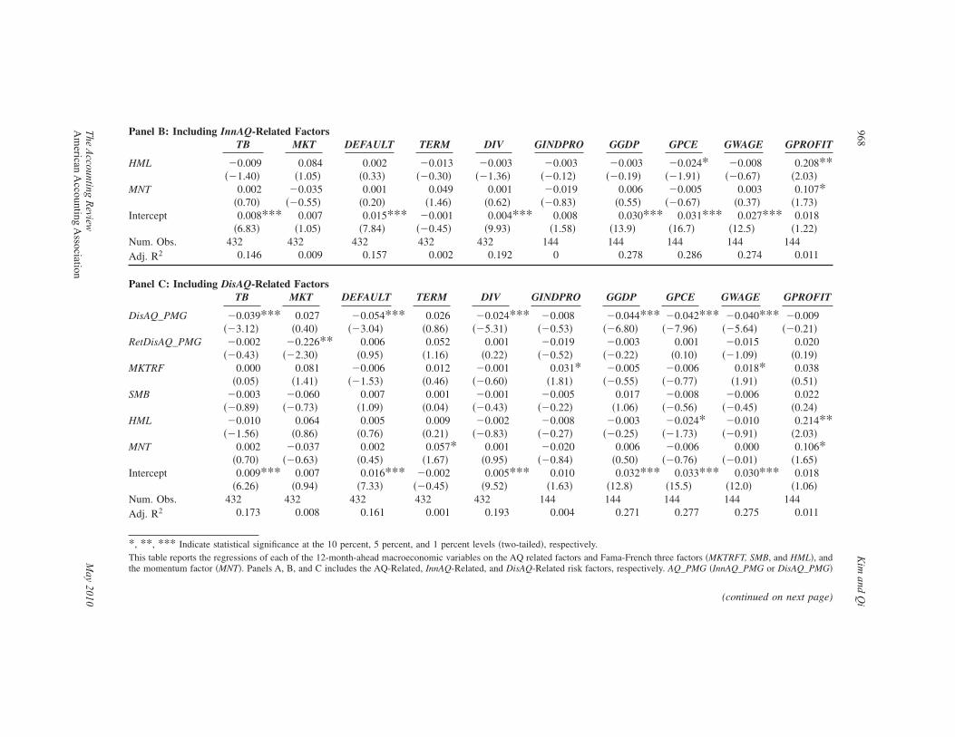
Panel B: Including InnAQ-Related FactorsTB MKT DEFAULT TERM DIV GINDPRO GGDP GPCE GWAGE GPROFIT

HML �0.009 0.084 0.002 �0.013 �0.003 �0.003 �0.003 �0.024* �0.008 0.208**��1.40� �1.05� �0.33� ��0.30� ��1.36� ��0.12� ��0.19� ��1.91� ��0.67� �2.03�

MNT 0.002 �0.035 0.001 0.049 0.001 �0.019 0.006 �0.005 0.003 0.107*�0.70� ��0.55� �0.20� �1.46� �0.62� ��0.83� �0.55� ��0.67� �0.37� �1.73�

Intercept 0.008*** 0.007 0.015*** �0.001 0.004*** 0.008 0.030*** 0.031*** 0.027*** 0.018�6.83� �1.05� �7.84� ��0.45� �9.93� �1.58� �13.9� �16.7� �12.5� �1.22�

Num. Obs. 432 432 432 432 432 144 144 144 144 144Adj. R2 0.146 0.009 0.157 0.002 0.192 0 0.278 0.286 0.274 0.011

Panel C: Including DisAQ-Related FactorsTB MKT DEFAULT TERM DIV GINDPRO GGDP GPCE GWAGE GPROFIT

DisAQ_PMG �0.039*** 0.027 �0.054*** 0.026 �0.024*** �0.008 �0.044*** �0.042*** �0.040*** �0.009��3.12� �0.40� ��3.04� �0.86� ��5.31� ��0.53� ��6.80� ��7.96� ��5.64� ��0.21�

RetDisAQ_PMG �0.002 �0.226** 0.006 0.052 0.001 �0.019 �0.003 0.001 �0.015 0.020��0.43� ��2.30� �0.95� �1.16� �0.22� ��0.52� ��0.22� �0.10� ��1.09� �0.19�

MKTRF 0.000 0.081 �0.006 0.012 �0.001 0.031* �0.005 �0.006 0.018* 0.038�0.05� �1.41� ��1.53� �0.46� ��0.60� �1.81� ��0.55� ��0.77� �1.91� �0.51�

SMB �0.003 �0.060 0.007 0.001 �0.001 �0.005 0.017 �0.008 �0.006 0.022��0.89� ��0.73� �1.09� �0.04� ��0.43� ��0.22� �1.06� ��0.56� ��0.45� �0.24�

HML �0.010 0.064 0.005 0.009 �0.002 �0.008 �0.003 �0.024* �0.010 0.214**��1.56� �0.86� �0.76� �0.21� ��0.83� ��0.27� ��0.25� ��1.73� ��0.91� �2.03�

MNT 0.002 �0.037 0.002 0.057* 0.001 �0.020 0.006 �0.006 0.000 0.106*�0.70� ��0.63� �0.45� �1.67� �0.95� ��0.84� �0.50� ��0.76� ��0.01� �1.65�

Intercept 0.009*** 0.007 0.016*** �0.002 0.005*** 0.010 0.032*** 0.033*** 0.030*** 0.018�6.26� �0.94� �7.33� ��0.45� �9.52� �1.63� �12.8� �15.5� �12.0� �1.06�

Num. Obs. 432 432 432 432 432 144 144 144 144 144Adj. R2 0.173 0.008 0.161 0.001 0.193 0.004 0.271 0.277 0.275 0.011

*, **, *** Indicate statistical significance at the 10 percent, 5 percent, and 1 percent levels �two-tailed�, respectively.This table reports the regressions of each of the 12-month-ahead macroeconomic variables on the AQ related factors and Fama-French three factors �MKTRFT, SMB, and HML�, andthe momentum factor �MNT�. Panels A, B, and C includes the AQ-Related, InnAQ-Related, and DisAQ-Related risk factors, respectively. AQ_PMG �InnAQ_PMG or DisAQ_PMG�


968K

imand

Qi

The

Accounting

Review

May

2010A

merican

Accounting

Association

is the difference of the AQ �InnAQ or DisAQ� values between the poorest and the best AQ decile portfolios. RetAQ_PMG �RetInnAQ_PMG or RetDisAQ_PMG� is the spread ofreturns between of the poorest and the best AQ �InnAQ or DisAQ� decile portfolios. InnAQ and DisAQ indicate the innate and discretionary portion of AQ, respectively. The financialmarket variables �TB, MKT, DEFAULT, TERM, and DIV� are in monthly frequency, and the real business environment variables �GINDPRO, GGDP, GPCE, GWAGE, and GPROFIT�are in quarterly frequency. Numbers reported in parentheses are t-statistics based on Newey-West standard errors. The sample period covers January 1970 through December 2006.


TB � return of the three-month Treasury Bill;MKT � return of the CRSP value-weighted market portfolio;

DEFAULT � default spread between Moody’s Baa corporate bond yield and Aaa corporate bond yield;TERM � term spread between ten-year government bond yields and three-month Treasury bill yields;

DIV � dividend yield of the CRSP market index of NYSE, AMEX, and NASDAQ listed firms;GINDPRO � growth rate of industrial production index;

GGDP � growth rate of GDP;GPCE � growth rate of personal consumption expenditure;

GWAGE � growth rate of employee compensation; andGPROFIT � growth rate of corporate profits.

Accruals

Quality,Stock

Returns,and

Macroeconom

icC

onditions969

The

Accounting

Review

May

2010A

merican

Accounting

Association

VI. CONCLUSIONSThis study contributes to the ongoing debate on whether AQ is priced in capital markets

�Francis et al. 2005 �FLOS�; Core et al. 2008 �CGV�; Ogneva 2008�. We re-examine the relation-ship between AQ and stock returns in two-stage CSR tests by controlling for low-priced returns.The reason we control for low-priced returns is that realized returns of low-priced stocks arenotoriously biased due to unsystematic factors such as noise trading, sentiment trading, andmarket-microstructure induced effects. Therefore, even if the relation between AQ and expectedreturns exists, it would be difficult to detect such a pricing relation in low-priced returns. We findin CSR tests using individual stocks that the AQ risk premium is statistically and economicallysignificant after controlling for low-priced returns. These results are robust for various beta esti-mation methods and portfolio formations. In particular, when assigned betas are used in the CSR,the AQ risk factor is statistically significant even without controlling for low-priced returns.Among the many risk factors considered, the AQ risk factor is the only one whose economic andstatistical significance is changed drastically after controlling for low-priced returns. However, theeconomic and statistical significance of the other risk factors remains relatively unchanged evenafter controlling for low-priced returns. Thus, CGV’s results that AQ is not significantly priced areseverely affected by low-priced returns.

This study also contributes to a broader stream of literature on earnings quality. We show thatthe AQ and its pricing effect are related to fundamental risk. We find that the return of AQ �i.e., therisk premium associated with AQ� react systematically to business cycles and macroeconomicconditions. Firms with poorer AQ are more exposed to macroeconomic shocks. More importantly,only the innate portion of AQ varies with macroeconomic conditions; the discretionary portion ofAQ does not. Therefore, only the innate portion of earnings quality is related to economy-widefundamental risk, and only this portion of AQ demonstrates the pricing effect on stock returns.These results support the argument that AQ is related to fundamental risk, with its pricing effect onexpected returns stemming from the innate component of AQ.

We also find that the risk premium of AQ and the dispersion of AQ between firms withpoorest and best earnings quality are significantly negatively related to future economic activity. Inaddition, the discretionary portion of AQ has predictive power on future economic activity similarto the innate portion of AQ. This predictive power may stem from earnings management andmanagement discretion that reflect management’s expectations for future economic conditions.

970 Kim and Qi


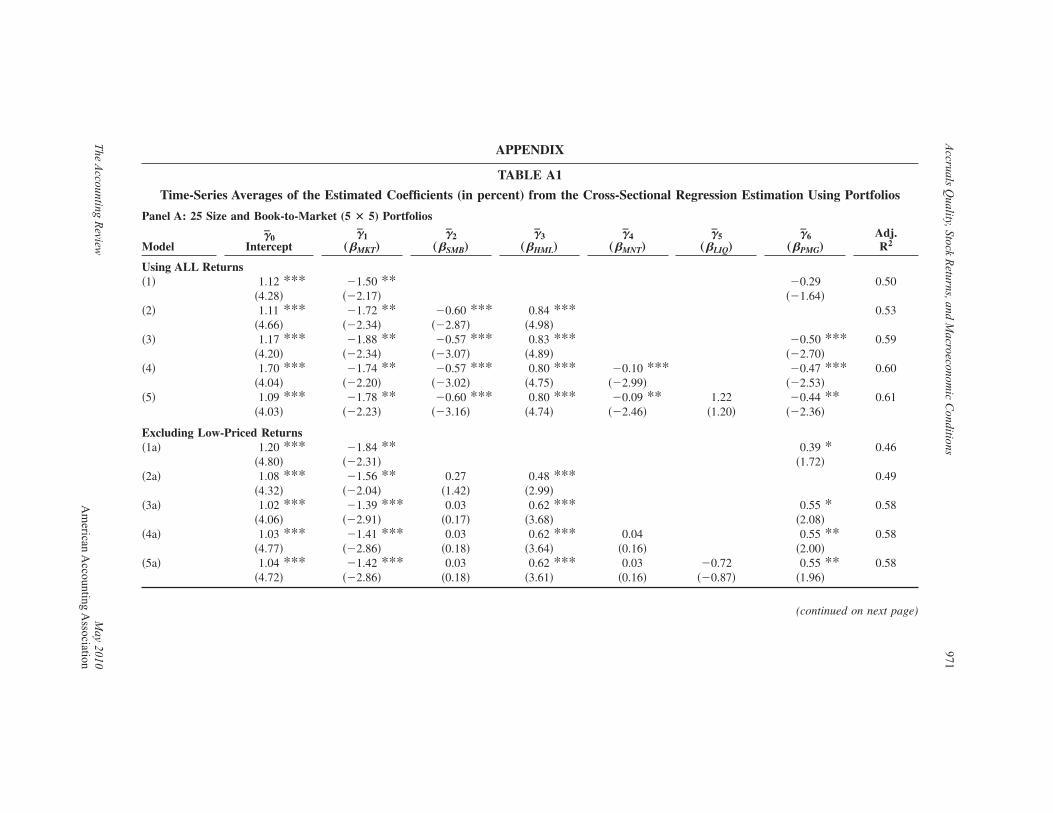
APPENDIX

TABLE A1

Time-Series Averages of the Estimated Coefficients (in percent) from the Cross-Sectional Regression Estimation Using Portfolios

Panel A: 25 Size and Book-to-Market (5 � 5) Portfolios

Model�̄0

Intercept�̄1

„�MKT…

�̄2„�SMB…

�̄3„�HML…

�̄4„�MNT…

�̄5„�LIQ…

�̄6„�PMG…

Adj.R2

Using ALL Returns�1� 1.12 *** �1.50 ** �0.29 0.50

�4.28� ��2.17� ��1.64��2� 1.11 *** �1.72 ** �0.60 *** 0.84 *** 0.53

�4.66� ��2.34� ��2.87� �4.98��3� 1.17 *** �1.88 ** �0.57 *** 0.83 *** �0.50 *** 0.59

�4.20� ��2.34� ��3.07� �4.89� ��2.70��4� 1.70 *** �1.74 ** �0.57 *** 0.80 *** �0.10 *** �0.47 *** 0.60

�4.04� ��2.20� ��3.02� �4.75� ��2.99� ��2.53��5� 1.09 *** �1.78 ** �0.60 *** 0.80 *** �0.09 ** 1.22 �0.44 ** 0.61

�4.03� ��2.23� ��3.16� �4.74� ��2.46� �1.20� ��2.36�

Excluding Low-Priced Returns�1a� 1.20 *** �1.84 ** 0.39 * 0.46

�4.80� ��2.31� �1.72��2a� 1.08 *** �1.56 ** 0.27 0.48 *** 0.49

�4.32� ��2.04� �1.42� �2.99��3a� 1.02 *** �1.39 *** 0.03 0.62 *** 0.55 * 0.58

�4.06� ��2.91� �0.17� �3.68� �2.08��4a� 1.03 *** �1.41 *** 0.03 0.62 *** 0.04 0.55 ** 0.58

�4.77� ��2.86� �0.18� �3.64� �0.16� �2.00��5a� 1.04 *** �1.42 *** 0.03 0.62 *** 0.03 �0.72 0.55 ** 0.58

�4.72� ��2.86� �0.18� �3.61� �0.16� ��0.87� �1.96�


Accruals

Quality,Stock

Returns,and

Macroeconom

icC

onditions971

The

Accounting

Review

May

2010A

merican

Accounting

Association

Panel B: 100 AQ Portfolios

Model�̄0

Intercept�̄1

„�MKT…

�̄2„�SMB…

�̄3„�HML…

�̄4„�MNT…

�̄5„�LIQ…

�̄6„�PMG…

Adj.R2

Using ALL Returns�1� 0.24 0.59 0.15 0.15

�0.70� �1.36� �0.89��2� �0.05 0.75 * 0.17 0.04 0.15

��0.15� �1.76� �0.78� �0.15��3� 0.03 0.70 0.05 0.13 0.15 0.17

�0.07� �1.63� �0.22� �0.53� �0.91��4� 0.19 0.70 �0.04 0.16 0.75 * 0.16 0.17

�0.51� �1.63� ��0.18� �0.63� �1.76� �0.94��5� 0.20 0.73 * �0.05 0.12 0.78 * �0.41 0.16 0.17

�0.53� �1.70� ��0.22� �0.47� �1.84� ��0.75� �0.95�

Excluding Low-Priced Returns�1a� 0.72 ** 0.08 0.58 *** 0.15

�2.39� �0.19� �3.09��2a� 0.68 ** 0.08 0.54 ** �0.40 0.15

�2.09� �0.19� �2.36� ��1.31��3a� 0.70 ** 0.05 0.45 * �0.15 0.57 *** 0.16

�2.12� �0.12� �1.85� ��0.53� �2.96��4a� 0.68 ** 0.11 0.42 * �0.12 0.22 0.56 *** 0.16

�2.07� �0.27� �1.70� ��0.40� �0.48� �2.91��5a� 0.68 ** 0.11 0.42 * �0.12 0.22 0.04 0.56 *** 0.17

�2.06� �0.27� �1.70� ��0.39� �0.48� �0.06� �2.88�

Panel C: 64 Size, Book-to-Market, and AQ (4 � 4 � 4) Portfolios

Model�̄0

Intercept�̄1

„�MKT…

�̄2„�SMB…

�̄3„�HML…

�̄4„�MNT…

�̄5„�LIQ…

�̄6„�PMG…

Adj.R2

Using ALL Returns�1� 2.29 *** �3.50 *** �0.07 0.19

�6.77� ��4.89� ��0.39��2� 1.11 * �1.29 0.25 0.84*** 0.21


972K

imand

Qi

The

Accounting

Review

May

2010A

merican

Accounting

Association

Panel C: 64 Size, Book-to-Market, and AQ (4 � 4 � 4) Portfolios

Model�̄0

Intercept�̄1

„�MKT…

�̄2„�SMB…

�̄3„�HML…

�̄4„�MNT…

�̄5„�LIQ…

�̄6„�PMG…

Adj.R2

�1.91� ��1.11� �1.00� �4.80��3� 1.01 * �0.90 0.06 0.90 *** �0.03 0.24

�1.68� ��0.74� �0.28� �4.99� ��0.15��4� 1.58 *** �1.92 * �0.02 0.61 *** �0.21 *** �0.05 0.27

�3.44� ��1.94� ��0.11� �3.31� ��2.59� ��0.25��5� 1.36 *** �1.80 * 0.02 0.58 *** �0.24 *** 0.38 �0.02 0.30

�3.47� ��1.84� �0.10� �3.25� ��2.97� �0.47� ��0.10�

Excluding Low-Priced Returns�1a� 1.89 *** �2.94 *** 0.35 * 0.15

�6.80� ��4.53� �1.75��2a� 0.98 *** �1.00 0.36 * 0.57 *** 0.18

�3.43� ��1.35� �1.98� �3.44��3a� 1.06 *** �1.16 0.21 0.69 *** 0.40 ** 0.20

�3.75� ��1.60� �1.11� �4.06� �2.02��4a� 0.98 *** �0.97 0.26 0.62 *** �0.13 ** 0.44 ** 0.21

�3.47� ��1.31� �1.41� �3.65� ��2.50� �2.23��5a� 1.16 *** �0.81 0.27 0.65 *** �0.19 *** �1.07 * 0.44 ** 0.22

�3.98� ��1.12� �1.46� �3.78� ��3.03� ��1.65� �2.22�

Panel D: 100 Size and Book-to-Market (10 � 10) Portfolios

Model�̄0

Intercept�̄1

„�MKT…

�̄2„�SMB…

�̄3„�HML…

�̄4„�MNT…

�̄5„�LIQ…

�̄6„�PMG…

Adj.R2

Using ALL Returns�1� 0.95 ** �1.21 ** �0.23 0.29

�2.28� ��2.25� ��1.28��2� 0.48 * �1.46 ** �0.23 0.88 *** 0.30

�1.90� ��2.58� ��1.11� �5.16��3� 0.23 * �1.74 ** �0.39 ** 0.94 *** �0.26 0.34

�1.91� �2.35� ��2.18� �5.43� ��1.40��4� 0.13 �1.16 *** �0.37 ** 0.86 *** �0.24*** �0.27 0.35


Accruals

Quality,Stock

Returns,and

Macroeconom

icC

onditions973

The

Accounting

Review

May

2010A

merican

Accounting

Association

Panel D: 100 Size and Book-to-Market (10 � 10) Portfolios

Model�̄0

Intercept�̄1

„�MKT…

�̄2„�SMB…

�̄3„�HML…

�̄4„�MNT…

�̄5„�LIQ…

�̄6„�PMG…

Adj.R2

�1.37� ��2.69� ��2.07� �5.04� ��5.17� ��1.48��5� 0.54 ** �1.20 *** �0.39 ** 0.86 *** �0.12 *** 1.32 ** �0.24 0.35

�2.35� ��2.74� ��2.16� �5.03� ��4.82� �2.00� ��1.35�

Excluding Low-Priced Returns�1a� 1.09 *** �1.53 ** 0.36 * 0.26

�2.67� ��2.20� �1.67��2a� 0.81 *** �1.91 *** 0.28 0.49 *** 0.28

�2.83� ��2.76� �1.49� �3.00��3a� 0.73 ** �1.74 *** 0.08 0.62 *** 0.50 ** 0.32

�2.44� ��2.60� �0.44� �3.63� �2.00��4a� 0.78 ** �1.86 *** 0.09 0.60 *** 0.03 0.45 * 0.33

�2.58� ��2.84� �0.51� �3.53� �1.26� �1.75��5a� 0.91 *** �1.88 *** 0.09 0.60 *** 0.02 �1.11 ** 0.43 * 0.33

�2.76� ��2.85� �0.50� �3.49� �1.20� ��1.97� �1.67�

Panel E: 100 Size Portfolios

Model�̄0

Intercept�̄1

„�MKT…

�̄2„�SMB…

�̄3„�HML…

�̄4„�MNT…

�̄5„�LIQ…

�̄6„�PMG…

Adj.R2

Using ALL Returns�1� 1.36 *** �0.83 *** 0.35 * 0.31

�4.50� ��2.78� �1.66��2� 3.46 *** �2.62 *** 0.11 �0.48 * 0.32

�5.94� ��4.32� �0.63� ��1.73��3� 1.15 *** �0.38 �0.10 �0.85 *** 0.78 *** 0.33

�3.43� ��0.98� ��0.06� ��3.16� �3.60��4� 1.26 *** �0.60 �0.04 �0.90 *** �0.86 ** 0.77 *** 0.34

�3.71� ��1.53� ��0.21� ��3.28� ��2.29� �3.56��5� 1.06 *** �0.41 0.05 �0.89 *** �0.53 1.86 *** 0.70 *** 0.34

�3.19� ��1.05� �0.27� ��3.27� ��1.44� �3.58� �3.24�


974K

imand

Qi

The

Accounting

Review

May

2010A

merican

Accounting

Association

Panel E: 100 Size Portfolios

Model�̄0

Intercept�̄1

„�MKT…

�̄2„�SMB…

�̄3„�HML…

�̄4„�MNT…

�̄5„�LIQ…

�̄6„�PMG…

Adj.R2

Excluding Low-Priced Returns�1a� 2.41 *** �1.72 *** 0.14 0.25

�7.98� ��4.62� �0.55��2a� 2.52 *** �1.89 *** �0.01 0.76 *** 0.26

�7.65� ��4.78� ��0.06� �3.21��3a� 2.31 *** �1.68 *** �0.02 0.75 *** �0.12 0.27

�8.95� ��5.01� ��0.10� �3.19� ��0.48��4a� 2.41 *** �1.82 *** �0.01 0.74 *** �0.39 �0.11 0.28

�9.24� ��5.40� ��0.03� �3.14� ��1.20� ��0.47��5a� 2.40 *** �1.82 *** �0.00 0.74 *** �0.38 �0.62 �0.12 0.28

�9.36� ��5.43� ��0.03� �3.13� ��1.18� ��1.42� ��0.47�

Panel F: Individual Stocks (all 23,634 firms)

Model�̄0

Intercept�̄1

„�MKT…

�̄2„�SMB…

�̄3„�HML…

�̄4„�MNT…

�̄5„�LIQ…

�̄6„�PMG…

Adj.R2

Using ALL Returns�1� 0.37 *** 0.47 ** 0.11 0.054

�3.11� �2.06� �0.63��2� 0.35 *** 0.43 * 0.17 �0.17 0.066

�3.35� �1.92� �0.96� ��1.08��3� 0.38 *** 0.43 * 0.17 �0.19 0.13 0.081

�3.83� �1.89� �1.02� ��1.22� �0.75��4� 0.37 *** 0.45 ** 0.18 �0.18 0.36 * 0.14 0.090

�3.85� �2.00� �1.10� ��1.17� �1.66� �0.83��5� 0.41 *** 0.41 * 0.18 �0.17 0.36 * 0.03 0.14 0.099

�4.43� �1.86� �1.08� ��1.10� �1.66� �0.12� �0.82�

Excluding Low-Priced Returns�1a� 0.52 *** 0.50 ** 0.31 * 0.07

�4.62� �2.20� �1.89��2a� 0.55 *** 0.45 ** 0.31 * �0.29 * 0.08


Accruals

Quality,Stock

Returns,and

Macroeconom

icC

onditions975

The

Accounting

Review

May

2010A

merican

Accounting

Association

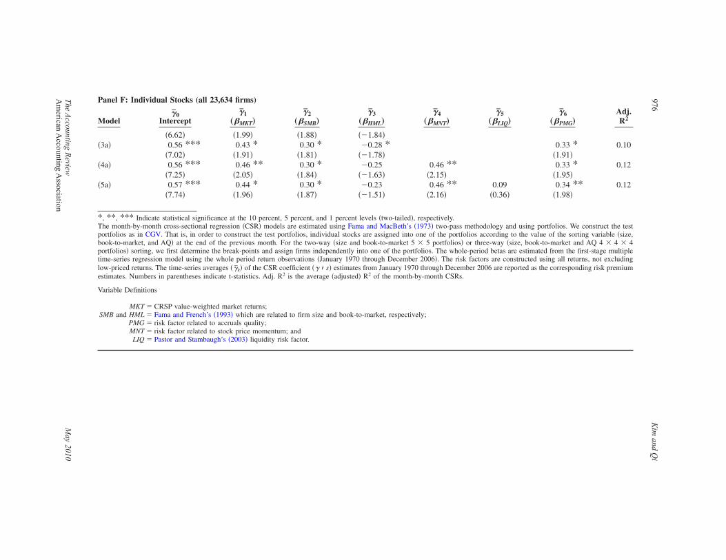
Panel F: Individual Stocks (all 23,634 firms)

Model�̄0

Intercept�̄1

„�MKT…

�̄2„�SMB…

�̄3„�HML…

�̄4„�MNT…

�̄5„�LIQ…

�̄6„�PMG…

Adj.R2

�6.62� �1.99� �1.88� ��1.84��3a� 0.56 *** 0.43 * 0.30 * �0.28 * 0.33 * 0.10

�7.02� �1.91� �1.81� ��1.78� �1.91��4a� 0.56 *** 0.46 ** 0.30 * �0.25 0.46 ** 0.33 * 0.12

�7.25� �2.05� �1.84� ��1.63� �2.15� �1.95��5a� 0.57 *** 0.44 * 0.30 * �0.23 0.46 ** 0.09 0.34 ** 0.12

�7.74� �1.96� �1.87� ��1.51� �2.16� �0.36� �1.98�

*, **, *** Indicate statistical significance at the 10 percent, 5 percent, and 1 percent levels �two-tailed�, respectively.The month-by-month cross-sectional regression �CSR� models are estimated using Fama and MacBeth’s �1973� two-pass methodology and using portfolios. We construct the testportfolios as in CGV. That is, in order to construct the test portfolios, individual stocks are assigned into one of the portfolios according to the value of the sorting variable �size,book-to-market, and AQ� at the end of the previous month. For the two-way �size and book-to-market 5 � 5 portfolios� or three-way �size, book-to-market and AQ 4 � 4 � 4portfolios� sorting, we first determine the break-points and assign firms independently into one of the portfolios. The whole-period betas are estimated from the first-stage multipletime-series regression model using the whole period return observations �January 1970 through December 2006�. The risk factors are constructed using all returns, not excludinglow-priced returns. The time-series averages ��̄k� of the CSR coefficient �� s� estimates from January 1970 through December 2006 are reported as the corresponding risk premiumestimates. Numbers in parentheses indicate t-statistics. Adj. R2 is the average �adjusted� R2 of the month-by-month CSRs.


MKT � CRSP value-weighted market returns;SMB and HML � Fama and French’s �1993� which are related to firm size and book-to-market, respectively;

PMG � risk factor related to accruals quality;MNT � risk factor related to stock price momentum; andLIQ � Pastor and Stambaugh’s �2003� liquidity risk factor.

976K

imand

Qi

The

Accounting

Review

May

2010A

merican

Accounting

Association

REFERENCES

Aboody, D., J. Hugher, and J. Liu. 2005. Earnings quality, insider trading, and cost of capital. Journal ofAccounting Research 43 �5�: 651–673.

Baker, M., and J. Wurgler. 2006. Investor sentiment and the cross-section of stocks returns. The Journal ofFinance 61 �4�: 1645–1680.

Bali, T. G., N. Cakici, X. Yan, and Z. Zhang. 2005. Does idiosyncratic risk really matter? The Journal ofFinance 60 �4�: 905–929.

Ball, R., S. P. Kothari, and J. Shanken. 1995. Problems in measuring portfolio performance: An applicationto contrarian investment strategies. Journal of Financial Economics 38 �1�: 79–107.

Bharath, S., J. Sunder, and S. Sunder. 2008. Accounting quality and debt contracting. The Accounting Review83 �1�: 1–28.

Bhardwaj, R. K., and L. D. Brooks. 1992. The January anomaly: Effects of low share price, transaction costs,and bid-ask-bias. The Journal of Finance 47 �2�: 553–575.

Botosan, C. 1997. Disclosure level and the cost of equity capital. The Accounting Review 72 �3�: 323–349.——–, and M. Plumlee. 2002. A re-examination of disclosure level and the expected cost of equity capital.

Journal of Accounting Research 40 �1�: 21–40.Chan, K., L. Chan, N. Jegadeesh, and J. Lakonishok. 2006. Earnings quality and stock returns. The Journal

of Business 79 �3�: 1041–1082.Chen, N. 1991. Financial investment opportunities and the macroeconomy. The Journal of Finance 46 �2�:

529–554.Chen, L. H., D. S. Dhaliwal, and M. A. Trombley. 2008. The effect of fundamental risk on the market pricing

of accruals quality. Journal of Accounting, Auditing & Finance 23 �4�: 1–29.Choi, J. 2008. An empirical study on the relationship between earnings quality and firm value. Asia-Pacific

Journal of Financial Studies 37 �5�: 813–839.Chordia, T., and L. Shivakumar. 2002. Momentum, business cycle, and time-varying expected returns. The

Journal of Finance 57 �2�: 985–1019.——–, and ——–. 2006. Earnings and price momentum. Journal of Financial Economics 80 �3�: 627–656.Conrad, J., and G. Kaul. 1993. Long-term market overreaction or biases in computed returns. The Journal of

Finance 48 �1�: 39–63.Cohen, D. 2008. Does information risk really matter? An analysis of the determinants and economic conse-

quences of financial reporting quality. Asia-Pacific Journal of Accounting and Economics 15 �2�:69–90.

Core, J., W. Guay, and R. Verdi. 2008. Is accruals quality a priced risk factor? Journal of Accounting andEconomics 46 �1�: 2–22.

Diamond, D., and R. Verrecchia. 1991. Disclosure, liquidity, and the cost of capital. The Journal of Finance46 �4�: 1325–1359.

Dechow, P., and I. Dichev. 2002. The quality of accruals and earnings: The role of accrual estimation errors.The Accounting Review 77 �1�: 35–59.

Easley, D., S. Hvidkjaer, and M. O’Hara. 2002. Is information risk a determinant of asset returns? TheJournal of Finance 57 �5�: 2185–2221.

——–, N. Kiefer, and M. O’Hara. 1997. One day in the life of a very common stock. Review of FinancialStudies 10 �3�: 805–835.

Ecker, F., J. Francis, I. Kim, P. Olsson, and K. Schipper. 2006. A returns-based representation of earningsquality. The Accounting Review 81 �4�: 749–780.

Epstein, L., and M. Schneider. 2008. Ambiguity, information quality, and asset pricing. The Journal ofFinance 63 �1�: 197–228.

Fama, E., and K. French. 1992. The cross section of expected stock returns. The Journal of Finance 47 �2�:427–465.

——–, and ——–. 1993. Common risk factors in the returns on stocks and bonds. Journal of FinancialEconomics 33 �1�: 3–56.

——–, and ——–. 1997. Industry cost of equity. Journal of Financial Economics 43 �2�: 153–193.——–, and J. MacBeth. 1973. Risk, return, and equilibrium: Empirical tests. The Journal of Political

Economy 81 �3�: 607–636.



http://dx.doi.org/10.1111/j.1475-679X.2005.00185.x


http://dx.doi.org/10.1111/j.1540-6261.2006.00885.x

http://dx.doi.org/10.1111/j.1540-6261.2006.00885.x

http://dx.doi.org/10.1111/j.1540-6261.2005.00750.x

http://dx.doi.org/10.1111/j.1540-6261.2005.00750.x

http://dx.doi.org/10.1016/0304-405X(94)00806-C

http://dx.doi.org/10.2308/accr.2008.83.1.1

http://dx.doi.org/10.2307/2329115

http://dx.doi.org/10.1111/1475-679X.00037

http://dx.doi.org/10.1086/500669

http://dx.doi.org/10.1086/500669

http://dx.doi.org/10.2307/2328835

http://dx.doi.org/10.1504/AJFA.2008.019876

http://dx.doi.org/10.1111/1540-6261.00449

http://dx.doi.org/10.1111/1540-6261.00449

http://dx.doi.org/10.1016/j.jfineco.2005.05.005

http://dx.doi.org/10.2307/2328881

http://dx.doi.org/10.2307/2328881

http://dx.doi.org/10.1016/j.jacceco.2007.08.001


http://dx.doi.org/10.2307/2328861

http://dx.doi.org/10.2308/accr.2002.77.s-1.35

http://dx.doi.org/10.1111/1540-6261.00493

http://dx.doi.org/10.1111/1540-6261.00493

http://dx.doi.org/10.1093/rfs/10.3.805



http://dx.doi.org/10.2307/2329112

http://dx.doi.org/10.1016/0304-405X(93)90023-5

http://dx.doi.org/10.1016/0304-405X(93)90023-5

http://dx.doi.org/10.1016/S0304-405X(96)00896-3

http://dx.doi.org/10.1086/260061

http://dx.doi.org/10.1086/260061

Francis, J., R. LaFond, P. Olsson, and K. Schipper. 2004. Cost of equity and earnings attributes. TheAccounting Review 79 �4�: 976–1010.

——–, ——–, ——–, and ——–. 2005. The market pricing of accruals quality. Journal of Accounting andEconomics 39 �2�: 295–327.

——–, P. Olsson, and K. Schipper. 2008. Earnings quality. Foundations and Trends in Accounting 1 �4�.Gray, P., P. Koh, and Y. H. Tong. 2009. Accruals quality, information risk and cost of capital: Evidence from

Australia. Journal of Business Finance & Accounting 36 �1&2�: 51–72.Guay, W., J. P. Kothari, and R. L. Watts. 1996. A market-based evaluation of discretionary accrual models.

Journal of Accounting Research 34 �Supplement�: 83–105.Hughes, J., J. Liu, and J. Liu. 2007. Information, diversification, and cost of capital. The Accounting Review

82 �3�: 705–729.Jegadeesh, N., and S. Titman. 1993. Returns to buying winners and selling losers: Implications for stock

market efficiency. The Journal of Finance 48 �1�: 65–91.——–, and ——–. 2001. Profitability of momentum strategies: An evaluation of alternative explanations. The

Journal of Finance 56 �2�: 699–720.Kim, D. 1995. The errors-in-variables problem in the cross-section of expected stock returns. The Journal of

Finance 50 �5�: 1905–1934.——– 1997. A reexamination of size, book-to-market, and earnings-price in the cross-section of expected

stock returns. Journal of Financial and Quantitative Analysis 32 �4�: 463–489.Lambert, R., C. Leuz, and R. Verrecchia. 2007. Accounting information, disclosure and the cost of capital.

Journal of Accounting Research 45 �2�: 385–420.——–, ——–, and ——–. 2008. Information asymmetry, information precision, and the cost of capital.

Working paper, University of Pennsylvania and The University of Chicago.Liew, J., and M. Vassalou. 2000. Can book-to-market, size and momentum be risk factors that predict

economic growth. Journal of Financial Economics 57 �2�: 221–245.Liu, M., and P. Wysocki. 2007. Cross-sectional determinants of information quality proxies and cost of

capital measures. Working paper, Pennsylvania State University and Massachusetts Institute of Tech-nology.

Lo, A., and A. C. MacKinlay. 1990. Data-snooping biases in tests of financial asset pricing models. Reviewof Financial Studies 3 �3�: 431–467.

McNichols, M. 2002. Discussion of the quality of accruals and earnings: The role of accrual estimationerrors. The Accounting Review 77 �1�: 61–69.

Merton, R. 1973. An intertemporal capital asset pricing model. Econometrica 41 �5�: 867–887.Ogneva, M. 2008. Accruals quality and expected returns: The importance of controlling for cash flow shocks.

Working paper, Stanford University.Pastor, L., and R. F. Stambaugh. 2003. Liquidity risk and expected stock returns. The Journal of Political

Economy 111 �3�: 642–685.Pontiff, J., and L. D. Schall. 1998. Book-to-market ratios as predictors of market returns. Journal of Finan-

cial Economics 49 �2�: 141–160.Ross, S. 1976. The arbitrage theory of capital asset pricing. Journal of Economic Theory 13 �3�: 341–360.Shanken, J. 1992. On the estimation of beta-pricing models. Review of Financial Studies 5 �1�: 1–33.Subramanyam, K. R. 1996. The pricing of discretionary accruals. Journal of Accounting Research 22 �1–3�:

249–281.Yee, K. K. 2006. Earnings quality and the equity risk premium: A benchmark model. Contemporary Account-

ing Research 23 �3�: 833–877.

978 Kim and Qi






http://dx.doi.org/10.1111/j.1468-5957.2008.02118.x

http://dx.doi.org/10.2307/2491427


http://dx.doi.org/10.2307/2328882

http://dx.doi.org/10.1111/0022-1082.00342

http://dx.doi.org/10.1111/0022-1082.00342

http://dx.doi.org/10.2307/2329328

http://dx.doi.org/10.2307/2329328

http://dx.doi.org/10.2307/2331233


http://dx.doi.org/10.1016/S0304-405X(00)00056-8



http://dx.doi.org/10.2308/accr.2002.77.s-1.61

http://dx.doi.org/10.2307/1913811

http://dx.doi.org/10.1086/374184

http://dx.doi.org/10.1086/374184

http://dx.doi.org/10.1016/S0304-405X(98)00020-8

http://dx.doi.org/10.1016/S0304-405X(98)00020-8

http://dx.doi.org/10.1016/0022-0531(76)90046-6


http://dx.doi.org/10.1506/8M44-W1DG-PLG4-8E0M

http://dx.doi.org/10.1506/8M44-W1DG-PLG4-8E0M

Copyright of Accounting Review is the property of American Accounting Association and its content may not

be copied or emailed to multiple sites or posted to a listserv without the copyright holder's express written

permission. However, users may print, download, or email articles for individual use.

accruals quality, stock returns, and macroeconomic conditions · pdf file ·...

Documents