Accounting for Mismatch Employment

Benedikt Herz and Thijs van Rens

No 1061

WARWICK ECONOMIC RESEARCH PAPERS

DEPARTMENT OF ECONOMICS

Accounting for Mismatch Unemployment

Benedikt HerzEuropean Commission∗

benedikt.herz@gmail.com

Thijs van RensUniversity of Warwick, Centre for Macroeconomics, IZA and CEPR

J.M.van-Rens@warwick.ac.uk, tvanrens@gmail.com

This version: May 2015†

First version: February 2011‡

Abstract

We investigate unemployment due to mismatch in the US over the past three

decades. We propose an accounting framework that allows us to estimate the over-

all amount of mismatch unemployment, as well as the contribution of each of the

frictions that caused the mismatch. Mismatch is quantitatively important for un-

employment and the cyclical behavior of mismatch unemployment is very similar

to that of the overall unemployment rate. Geographic mismatch is driven primarily

by wage frictions. Mismatch across industries is driven by wage frictions as well as

barriers to job mobility. We find virtually no role for worker mobility frictions.

Keywords: mismatch, structural unemployment, worker mobility, job mobility

JEL codes: E24 J61 J62

∗The views expressed in this paper are those of the authors and should not be attributed to theEuropean Commission.†We thank the following people for helpful comments and discussions: Árpád Ábrahám, Francesco

Amodio, Gadi Barlevy, Régis Barnichon, Björn Brügemann, Tomaz Cajner, Francesca Carapella, Car-los Carrillo Tudela, Vasco Carvalho, Briana Chang, Sekyu Choi, Larry Christiano, Antonio Ciccone,Melvyn Coles, Jim Costain, Steve Davis, Wouter Denhaan, Sijmen Duineveld, Monique Ebell, GiuliuFella, Shigeru Fujita, Jordi Galí, Pieter Gautier, Martin Gervais, Albrecht Glitz, Ai Ting Goh, LibertadGonzalez, Christian Haefke, Giammario Impullitti, Alejandro Justiniano, Philipp Kircher, MariannaKudlyak, Omar Licandro, Igor Livshits, Rafael Lopes de Melo, Ignacio Lopez, Thomas Lubik, IouriiManovskii, Alberto Martin, Guido Menzio, Pascal Michaillat, Tomasz Michalski, Claudio Michelacci,Giuseppe Moscarini, Kris Nimark, Nicola Pavoni, Nicolas Petrosky-Nadeau, Giacomo Ponzetto, Gior-gio Primiceri, Roland Rathelot, Richard Rogerson, Aysegül Sahin, Kurt Schmidheiny, Petr Sedlácek,Matthew Shapiro, Rob Shimer, Henry Siu, Eric Smith, Andrea Tambalotti, Giorgio Topa, LawrenceUren, Jaume Ventura, Gianluca Violante, Ludo Visschers, Etienne Wasmer, Sweder van Wijnbergenand our discussants Winfried Koeniger and Michael Reiter.‡Earlier versions of this paper were circulated under the title “Structural Unemployment”.

1

1 Introduction

After the end of the Great Recession in December 2007, unemployment in the United

States remained high for more than half a decade. One explanation that was suggested

is a mismatch in the skills or geographic location of the available jobs and workers, a

view that seemed to be supported by a decline in aggregate matching effi ciency (Elsby,

Hobijn, and Sahin (2010), Barnichon and Figura (2010)) and geographic mobility (Frey

(2009)). There was, however, little empirical work using disaggregated data to either

support or reject this hypothesis.

In this paper, we estimate mismatch unemployment on the US labor market, study

its evolution over time and explore what frictions caused mismatch to arise. To do so,

we use an accounting framework that puts just enough structure on the data to allow

us to quantify the sources of mismatch unemployment.

Our accounting framework models the labor market as consisting of multiple sub-

markets or segments. Mismatch is defined as dispersion in labor market conditions, in

particular the job finding rate, across labor market segments. Within segments, frictions

prevent the instantaneous matching of unemployed workers to vacant jobs, resulting in

search unemployment in the tradition of Diamond (1982), Mortensen (1982) and Pis-

sarides (1985). Across segments, frictions generate dispersion in labor market conditions,

which gives rise to mismatch unemployment. There are four types of frictions that gen-

erate mismatch: worker mobility costs, job mobility costs, wage setting frictions and

heterogeneity in matching effi ciency. Figure 1 visualizes the framework.

The data required to estimate mismatch unemployment and its sources using our

approach, are job and worker finding rates, and worker and job surplus by labor market

segments, which we operationalize as states or industries. We construct these variables

over the 1979-2009 period using data on worker flows and wages from the Current

Population Survey (CPS) and data on profits from the National Income and Product

Accounts (NIPA).

Consistent with other recent studies, we argue that mismatch is an important rea-

son for unemployment. A back-of-the-envelope calculation correcting our estimates for

aggregation bias suggests that mismatch is responsible for a large part of both the level

and the fluctuations in the unemployment rate. The cyclical behavior of mismatch un-

employment is very similar to that of the overall unemployment rate. This finding is

driven by the fact that dispersion in labor market conditions across states and industries

moves closely with the business cycle, similar to what Abraham and Katz (1986) docu-

mented over two decades ago.1 The unemployment that derives from this dispersion is

as cyclical as the overall unemployment rate and no more persistent. As a corollary, the

nature of the increase in unemployment in the Great Recession was no different from

1 In response to the structural shifts view of recessions put forward by Lilien (1982), which holds thatrecessions are periods of reallocation between industries akin to mismatch, Abraham and Katz showedthat aggregate shocks can give rise to countercyclical fluctuations in dispersion of employment growthacross sectors.

2

previous recessions, although it was of course more severe.2 We find no evidence that

mismatch unemployment is ‘structural’, in the sense that it would not be not responsive

to stabilization policy.3

Our most interesting and novel set of results concerns the sources of labor market

mismatch. We find that most mismatch is caused by dispersion in the share of surplus

that goes to workers, i.e. by wage setting ‘frictions’. Industries and states with high

wages tend to have low profits. This implies that those states and industries that are

attractive to workers are unattractive to firms, and vice versa. Little or no mismatch is

due to worker mobility frictions. These conclusions are based on the testing the strong

predictions generated by our framework for the patterns we should observe in the data

in the absence of the various frictions that can give rise to mismatch. In particular,

if there are no barriers to worker mobility, a no-arbitrage condition dictates that we

should see a negative correlation between wages (measuring how attractive it is to have

a job in a given state or industry) and job finding rates (how hard it is to find these

jobs). In the data, we find that deviations from this correlation are small and non-

systematic. An implication of these results is that policies aimed at increasing worker

mobility, as advocated e.g. by Katz (2010), are likely to have small effects and may even

be counterproductive.

The detailed empirical analysis we provide, indicates that it is fruitful to think of

mismatch as a possible micro-foundation for unemployment. In most modern macro-

economic models of the labor market there is unemployment because of search frictions.

But the micro-foundations for search frictions and the aggregate matching function are

not very well developed. If unemployment is truly due to a time cost of search, it seems

there should be a secular downward trend in the unemployment rate as computers and

the internet improve the search technology available to firms and workers. Instead,

we think of search frictions as “a modeling device that captures the implications of the

costly trading process without the need to make the heterogeneity and the other features

2This result is not inconsistent with observation that there was an outward shift in the Beveridgecurve, the negatively sloped relation between vacancies and unemployment, which indicates a declinein aggregate matching effi ciency and provides much of the basis for the argument that there was anunprecedented increase in mismatch in the Great Recession (Elsby, Hobijn, and Sahin (2010), Lubik(2013)). While an increase in mismatch indeed reduces matching effi ciency (Shimer (2007)), there aremany other causes for shifts in the Beveridge curve as well, including changes in the separation rate anddemographics. Controlling for these factors, the remaining role for mismatch is very small (Barnichonand Figura (2010)). For the same reason, our findings are not contradictory with the observationthat exogenous shocks to mismatch are not an important as a source of unemployment fluctuations(Furlanetto and Groshenny (2013)).

3 In the wake of the Great Recession, this was a widely held view, advocated most prominently byNarayana Kocherlakota (2010), the president of the Federal Reserve Bank of Minneapolis, who arguedthat “it is hard to see how the Fed can do much to cure this problem. Monetary stimulus has providedconditions so that manufacturing plants want to hire new workers. But the Fed does not have a meansto transform construction workers into manufacturing workers.” See Estevão and Tsounta (2011) andGroshen and Potter (2003) for versions of this argument. Early critics include Krugman (2010), DeLong(2010), Lazear and Spletzer (2012), and Peter Diamond (2011), who notes in his Nobel lecture that“there is a long history of claims that the latest technological or structural developments make for anew long-term high level of unemployment, but these have repeatedly been proven wrong.” (p.1065).Kocherlakota later changed his views in light of the evidence (New York Times (2014)).

3

that give rise to it explicit”(Pissarides (2000, p.4)). Mismatch generates heterogeneity

and therefore gives rise to unemployment. The results in this paper shed light on the

question what are the frictions that give rise to mismatch.4

Previous empirical studies on mismatch tend to focus on shifts in the Beveridge curve,

trying to use aggregate data to estimate matching effi ciency (Lipsey (1965), Abraham

(1987), Blanchard and Diamond (1989), Barnichon and Figura (2010)) and there is little

recent empirical work using disaggregated data.5 Two recent contributions, however, are

closely related to this paper. Sahin, Song, Topa, and Violante (2014) use disaggregated

data on unemployment and vacancies to construct indices of mismatch, using data from

the JOLTS and the HWOL for the 2001-2011 and 2005-2011 periods respectively. Bar-

nichon and Figura (2013) use the CPS to explore how much dispersion in labor market

conditions contributes to movements in matching effi ciency. Our findings are consistent

with these papers in terms of the contribution of mismatch across states and industries

to the increase in unemployment in the Great Recession.6 Compared to Sahin, Song,

Topa, and Violante (2014), we provide an alternative method to estimate mismatch un-

employment, which gives us a much longer time series. The longer series allows us to

better explore the cyclical behavior of mismatch unemployment. Compared to Barni-

chon and Figura (2013), our focus is on unemployment rather than matching effi ciency.

Our main contribution with respect to both papers is the accounting framework that

allows us to decompose mismatch into it sources and to estimate the contribution of

each of these sources to unemployment.

This paper is organized as follows. In the next section we present the accounting

framework to formalize the sources of dispersion in labor market conditions across sub-

markets of the labor market. We identify four sources of mismatch, three of which we

can estimate: worker mobility costs, job mobility costs and wage setting frictions. Sec-

tion 3 describes the data used in the estimation, and explains in detail how we construct

the empirical counterparts of the variables that define a labor market segment in our

model. Section 4 presents the empirical results and Section 5 concludes.

4Some recent studies discuss this issue from a theoretical perspective. Shimer (2007) formally showsthat mismatch between the distributions of workers and jobs over segments of the labor market gives riseto a relation between the job finding probability and labor market tightness that is very similar to therelation obtained if there are search frictions and an aggregate matching function. Stock-flow matching,as in Coles, Jones, and Smith (2010), rest unemployment, as in Alvarez and Shimer (2011), reallocationunemployment as in Carrillo-Tudela and Visschers (2013), Wong (2012) or Chang (2011), and waitingunemployment as in Birchenall (2011) are all closely related to this concept of unemployment due tomismatch. As opposed to these studies, the focus of our paper is empirical. One way to think aboutthe contribution of this paper is to provide a set of facts unemployment that can be used to test thetheoretical models of mismatch unemployment.

5Older studies include work by Padoa Schioppa (1991) and Phelps (1994).6The finding that geographic mismatch cannot explain why the increase in unemployment in the

Great Recession is so much larger than in previous recessions is also consistent with work by Kaplanand Schulhofer-Wohl (2011), who show that most of the a drop in interstate migration in the GreatRecession is a statistical artifact.

4

2 Accounting Framework

The theoretical framework presented here allows us to formalize the mechanisms, by

which heterogeneity in labor market conditions across submarkets of the labor market

leads to mismatch unemployment. In addition, we use the framework to guide the

empirical exercise how to estimate mismatch unemployment and how to decompose it

into its sources. We try to make as little assumptions as possible. In particular, we

do not assume anything about vacancy creation, but model only the distribution of

vacancies and unemployed workers over submarkets.

Unemployed workers look for jobs, and firms with vacancies look for unemployed

workers on the labor market. But not each unemployed worker can match with each

vacancy. We model this idea as a labor market that is segmented into submarkets. A

submarket is defined as the subset of jobs that a given unemployed worker searches for,

or the subset of unemployed workers that can form a match with a given vacancy. We

assume that there is a one-to-one mapping of the set of workers and firms that search

for each other, ruling out that workers or firms spread out their search effort over several

submarkets.7 In addition, we assume that in each submarket, there is a technology to

match unemployed workers with vacancies.8

Under these assumptions, labor market conditions in a submarket can be completely

characterized by four variables: the probability that an unemployed workers finds a job,

the increase in life-time earnings by a worker who finds a job, the probability that a

vacant job finds a worker, and the increase in life-time profits by a firm that fills a vacant

job. These four variables are the job finding rate fWi , worker surplus SWi , the job filling

rate or worker finding rate fFi and job surplus SFi in submarket i, respectively.

Any labor market model with a segmented labor market must describe how labor

market conditions are related across submarkets. We show which relations effectively

reduce the segmented labor market to a single market, as in the standard search and

matching model with homogeneous workers and jobs, in the tradition of Diamond (1982),

Mortensen (1982) and Pissarides (1985). We take these relations as a benchmark and

explore the effect of deviations from it. Unemployment that results under the benchmark

conditions may be due to a variety of frictions, for instance search frictions. We refer to

this unemployment as ‘frictional’. Unemployment that results from deviations from the

benchmark conditions (and is therefore due to dispersion in labor market conditions) is

called mismatch unemployment.

7This assumption is without loss of generality as long as the total amount of search effort is limited.It is, of course, diffi cult to operationalize this concept of a submarket empirically. In practice, we useeither states or industries in most of our estimates, which is a much higher level of aggregation comparedto the ideal. In Sections 2.2 and 4.2.1, we discuss how this affects our estimates.

8Our accounting framework is based on worker and job mobility arbitraging away differences in thevalue of searching in each submarket. In order for arbitrage to be possible, we need the (plausible)assumption that the matching technology has positive and diminishing returns in each of its inputs. Inother words, we assume that adding an additional unemployed worker to a submarket, ceteris paribus,makes it harder for workers to find jobs and easier for firms to fill vacancies (and similar for adding anadditional vacancy).

5

2.1 Benchmark Relations

The relation between the job finding rate fWi and worker surplus SWi across submarkets

is determined by assumptions about worker mobility between submarkets, the relation

between the worker finding rate fFi and job surplus SFi by assumptions about job mobil-

ity (mobility of vacancies), the relation between worker and job surplus by assumptions

about wage determination, and the relation between job and workers finding rates by

assumptions about the matching technology. These four relations, which are summa-

rized in Figure 1, fully determine conditions in submarkets of the labor market. We now

discuss each of these four relations in turn.

2.1.1 Worker Mobility

An unemployed worker, searching for a job in submarket i, receives an unemployment

benefit bWi (which, as usual, includes the utility from leisure). With probability fWi , this

worker finds a job, in which case she receives the worker surplus SWi from the match.

Thus, the per-period value of searching for a job in submarket i, assuming it is constant

over time, is given by zWi = bWi + fWi SWi .9

If workers may freely decide in which submarket to search, i.e. if there are no

barriers to worker mobility, it must be that the value of searching is equalized across

submarkets, so that zWi = zW for all i. Using a bar over a variable to denote its

mean over all submarkets and a hat to denote relative deviations from this mean, e.g.

fWi =(fWi − fW

)/fW , equalization of the value of searching in all submarkets implies

the following relation between fWi and SWi , which we label the worker mobility curve.10

fWi + SWi = − bW

zW − bWbWi (1)

Assuming unemployment benefits are the same in all submarkets, we get fWi = −SWi .The worker mobility curve is a no-arbitrage condition. It states that attractive jobs

must be hard, and unattractive jobs easy to find, in order for workers to be indifferent

which job they search for.11 If unemployment benefits differ across submarkets, then

submarkets with high unemployment benefits must have low job finding rates or low

worker surplus or both.

If there are barriers to worker mobility, for example because it is costly to move

9The assumption that zWi is in steady state seems reasonable, because average unemployment dura-tion, compared to the length of a typical business cycle, is short in the US.10The condition is exact for log-deviations but only a first-order approximation for relative deviations

from the mean. The same caveat applies to conditions (3), (4) and (5) below. The reason we neverthelessprefer relative deviations is because empirically log-deviations are problematic in the (rare) cases thatvariables are negative.11The insight is the same as that of the Harris and Todaro (1970) model of rural-urban migration.

In the context of worker mobility, it should not be surprising that some (urban) areas have muchlower job finding rates (higher unemployment) if wages are much higher there. Similarly, Montgomery(1991) prosposes differences in job finding rates as an explanation for persistent wage differentials acrossindustries.

6

from one state to another, or because moving into a different industry requires costly

retraining, then there may be differences in the value of searching across submarkets.

We denote these differences by αWMi , so that the worker mobility curve is given by

fWi + SWi = αWMi (2)

If unemployment benefits are the same across submarkets, the dispersion in αWMi is a

measure of worker mobility costs. If the difference in the value of searching in a particular

submarket i becomes to high compared to the average, it becomes worthwhile for workers

to pay the mobility cost and move into that submarket. Unemployed workers moving

into market i make it harder to find a job in that submarket, reducing fWi and therefore

αWMi . If unemployment benefits vary across submarkets, then differences in the value of

searching may also reflect differences in unemployment benefits, αWMi = − bW

zW−bW bWi .

2.1.2 Job Mobility

Having a vacancy looking for a worker in submarket i yields the firm bFi , which may be

a negative number, i.e. vacancy posting costs. With probability fFi , this vacancy gets

filled, in which case the firm gets surplus SFi from the match. Thus, the (steady state)

per-period value of searching for a worker in submarket i is given by zFi = bFi + fFi SFi .

If firms can freely relocate vacancies across submarkets, no-arbitrage requires that

the value of searching for a worker must be equal across submarkets. Analogous to

the worker mobility curve, we get a job mobility curve, which states that jobs that are

attractive to firms must be hard to fill. If there are barriers to job mobility, these give

rise to differences in the value of a vacancy across submarkets.

fFi + SFi = αJMi (3)

Dispersion in αJMi may reflect job mobility costs and/or dispersion in vacancy posting

costs, αJMi = − bF

zF−bF bFi .

2.1.3 Wage Determination

The relation between worker and firm surplus is determined by assumptions on how

worker and firm divide the total surplus from their match. The instrument that is used

to divide the surplus is the wage. In our benchmark relation, which is the only relation

that does not give rise to any mismatch, firm and worker share the surplus in fixed

proportions across segments. This relation would be true in standard labor market

models, which commonly assume that wages are set by generalized Nash bargaining.

Here, however, we are not making any specific assumptions on the wage determination

process, but merely stating a benchmark relation for surplus sharing that does not give

rise to mismatch.

If the share of match surplus that goes to the worker φi, often referred to as the

7

worker’s bargaining power, is constant across submarkets, then worker and job surplus

are proportional across submarkets, SWi = SJi . In general, wages may deviate from this

benchmark relation, for example because bargaining power varies across segments or

because wages are not rebargained in each period. This is captured by deviations from

the wage determination curve.

SWi = SFi + αWDi (4)

Dispersion in αWDi may reflect wage bargaining costs or heterogeneity in workers bar-

gaining power, αWDi = φi

1−φi , but may also reflect that wages are determined by a

completely different mechanism than bargaining. In the interest of brevity, we refer to

deviations from the benchmark wage determination curve as evidence for wage setting

‘frictions’.

2.1.4 Matching Technology

The final relation needed to close the model, between worker and job finding rates,

is determined by assumptions on the matching technology. In our benchmark rela-

tion, the probability that workers find jobs and the probability that firms find workers

are inversely log-proportional. This is true, for instance, if matches are formed from

unemployed workers and vacancies through a constant returns to scale Cobb-Douglas

matching function. Under this assumption, the worker and job finding rates are both

iso-elastic functions of the vacancy-unemployment ratio θi, often referred to as labor

market tightness, fFi = Biθ−µi and fWi = Biθ

1−µi , where µ is the elasticity of unem-

ployment in the matching function and Bi is matching effi ciency. This gives rise to the

following curve, describing the matching process.

fFi = − µ

1− µfWi + αMT

i (5)

Dispersion in αMTi reflects dispersion in matching effi ciency across submarkets, αMT

i =Bi

1−µ . If the elasticity of the matching function is not constant across submarkets, then

the above relation still holds in first order approximation, and αMTi reflects all differences

in the matching function across submarkets, αMTi = Bi

1−µ −µ

1−µ(fW − fF

)µi.

Our data do not allow us to test the benchmark relation on the matching technology.

Therefore, in the empirical work we will assume that αMTi = 0 for all i. There is some

evidence from other data sources that this assumption may not be too far from the truth

(Sahin, Song, Topa, and Violante (2014)), see Section 3.2 for a short discussion. In the

description of the framework in this section, we will allow for αMTi to be non-zero for

completeness.

8

2.2 Mismatch Unemployment

Combine equations (2), (3), (4) and (5) to solve for the distribution of job finding rates

across segments.

fWi = (1− µ)(αWMi − αJMi − αWD

i + αMTi

)(6)

Note that the benchmark relations were defined so that only deviations from these equa-

tions give rise to dispersion in labor market conditions. If there is perfect worker mobil-

ity, perfect job mobility, wages are set to share match surplus in constant proportions,

and there is a matching function with constant matching effi ciency, then labor market

conditions are identical in all submarkets: setting αWMi = αJMi = αWD

i = αMFi = 0 in

equation (6) gives fWi = 0 or fWi = fW for all i. Substituting back into the various

equations, it is straightforward to show that the worker finding rate, and worker and firm

surplus are equalized as well. In this case, the model reduces to a standard labor market

model, in which we can effectively think of the labor market as a single, unsegmented

market. Unemployment in this case is entirely due to frictions within submarkets, e.g.

search frictions.

Dispersion in labor market conditions generates unemployment because the job find-

ing rate is concave in labor market tightness. Therefore, the distribution of vacancies

and unemployed workers that results in the highest aggregate job finding rate, keep-

ing fixed the total number of vacancies and unemployed, is to equalize labor market

tightness over submarkets. To formalize this, consider a mean-preserving change in the

distribution of labor market tightness from θi to θ′i. The counterfactual unemployment

rate uCF that prevails under the new distribution is given by,

uCF

u' fW

fW,CF=

E[(

1 + fW,CFi

) 11−µ]

E

[(1 + fWi

) 11−µ]

1−µ

∝V[θCFi /θCF

]V[θi/θ

] (7)

where 0 < µ < 1 is the elasticity of unemployment in the matching function. See

appendix A for the derivation of equation (7). The aggregate job finding rate is higher

and therefore the unemployment rate lower, uCF < u, if and only if the dispersion in

fW,CFi is smaller than the dispersion in fWi , in the sense that θi is a mean-preserving

spread of θCFi (i.e. the distribution of θCFi second-order stochastically dominates the

distribution of θi).12

To calculate the contribution of mismatch to unemployment, we use the actual job

finding rates for fWi and set the counterfactual finding rates fW,CFi = 0 to represent

the full equalization of labor market conditions that would prevail in the absence of

mismatch. Then,(u− uCF

)/u is the fraction of unemployment that is due to mismatch.

The importance of mismatch estimated in this manner will depend on the time period as

12The first approximation is just for ease of interpretation. In the empirical work, we calculate thecounterfactual job finding rate using (7) and then calculate the counterfactual steady state unemploy-ment rate as u = λ/ (λ+ f).

9

well as on the level of disaggregation. Benchmark conditions (2), (3) and (4) assume the

labor market is in steady state. Given the speed of transition dynamics in unemployment

and the fact that we use annual data, we do not expect the results to be affected very

much by this assumption. However, to the extent that some of the adjustment may not

yet have been realized, our estimates provide an upper bound for the amount of mismatch

due to each source. The effect of the level of disaggregation is more important. At higher

levels of aggregation, we would expect to see substantial mismatch within segments,

so that the observed mismatch across segments is a lower bound for the actual labor

market mismatch. We return to this issue in detail when we discuss the overall amount

of mismatch in Section 4.2.1.

2.3 Mismatch Accounting

Deviations from any of the four benchmark relations generate dispersion in labor market

tightness and job finding rates. There are four sources of dispersion across submarkets of

the labor market: αWMi represents heterogeneity in unemployment benefits and barriers

to worker mobility, αJMi heterogeneity in vacancy posting costs and barriers to job mo-

bility, αWDi heterogeneity in wage bargaining power or other wage setting frictions, and

αMTi heterogeneity in matching effi ciency. All four sources lead to unemployed workers

and vacancies being in different submarkets and thus cause mismatch unemployment.

For example, if αWMi > 0, too few unemployed workers are searching for jobs in submar-

ket i, either because unemployment benefits are relatively low there or because mobility

costs prevent more unemployed workers from moving into that submarket. If αWDi > 0,

too many unemployed workers and too few vacancies are in submarket i, because wages

are higher (and profits lower) than in comparable jobs in other submarkets so that

workers reap a disproportionately large share of match surplus in this submarket.

Equations (6) and (7) allow us to decompose mismatch unemployment into its four

sources. The idea is that if we remove, for example, the worker mobility frictions, setting

αWMi = 0, but leave the job mobility frictions, wage setting frictions, and heterogeneity

in matching effi ciency in place, then αJMi , αWDi and αMT

i would stay the same. Notice

that this is probably not a good assumption for the short run, because worker or job

mobility or wage renegotiations affect equations (2), (3) and (4) simultaneously. In

the long run, however, after many shocks have hit the labor market, we would expect

deviations because of job mobility, wage setting frictions, or heterogeneity in matching

effi ciency to be similar to what they were. Thus, the question we can answer is what

unemployment rate would prevail in the long run, if we removed one or more deviations

from the benchmark model.

The procedure to decompose mismatch unemployment into its sources is imple-

mented in three steps. First, we estimate the α’s using equations (2), (3), (4) and (5)

and data on the surpluses and finding rates (section 3 below describes how we obtain

these data). Second, given estimates for αWMi , αJMi , αWD

i and αMTi , we use equation (6)

to calculate what the job finding rates in each submarket would be if we set one or more

10

of the α ’s equal to zero. Finally, using equation (7), we calculate the unemployment

rate that would prevail under these scenarios. We refer to this exercise as mismatch

accounting.

The last step of the decomposition is always relative to a baseline level of unemploy-

ment, see equation (7). This means we can always estimate the contribution of each

source in two different ways, introducing the friction with respect to a baseline, in which

the friction was absent, or removing the friction with respect to a baseline, in which

it was present. In general, the two approaches will give different answers because the

alpha’s may be correlated.13 More importantly, the contribution of each friction will

depend on the order in which we introduce or remove the various frictions. In appendix

B, we show that the contribution of a friction that we remove includes the contribution

of the covariance of that friction with other frictions in place, whereas the contribution

of a friction that we introduce does not. Therefore, we calculate the contribution of

each friction in both ways and average it, attributing the covariance between two fric-

tions in equal proportions to each of the frictions. This way, we make sure that our

decomposition adds up to the total amount of mismatch unemployment.

2.4 Discussion

Before turning to the data, we briefly discuss a few conceptual issues with the mismatch

accounting procedure and compare our approach to the other studies in the (small)

recent literature on labor market mismatch. First and foremost, we want to emphasize

that we are not taking a stance ex-ante on whether or not we expect the benchmark

conditions on worker mobility (2), job mobility (3), and wage determination (4) to be

satisfied in the data. These conditions are just benchmark conditions: conditions, under

which labor market conditions are fully equalized across segments. Deviations from the

benchmark conditions represent sources of labor market mismatch.

The benchmark conditions on wage determination (4) and matching technology (5)

are of a different nature than the conditions for worker mobility (2) and job mobility

(3). The latter are no-arbitrage conditions, and deviations from these conditions have a

straightforward interpretation as evidence for barriers to worker or job mobility across

segments. The interpretation of deviations from the wage determination and matching

technology conditions is less straightforward. Consequently, one could have a semantic

debate whether dispersion in labor market conditions originating from deviations from

these conditions should even be labeled as ‘mismatch’. Our pragmatic solution to this

13Note that this also means that removing one or more of these sources of mismatch does not nec-essarily decrease unemployment as the different frictions may reinforce or counteract each other. Thisresult is intuitive. Imagine two otherwise identical submarkets of the labor market, one with high wagesand one with low wages. Suppose these wage differentials can exist because of wage setting frictions,but that labor market tightness is nevertheless equal in both submarkets, because mobility costs preventworkers and jobs from moving from one submarket to the other. Now suppose we removed the mobilitycosts but left the wage setting frictions in place. Unemployed workers would move to the submarketwhere wages are high, whereas vacancies would move to the submarket where wages are low. The resultwould be a decrease in the aggregate job finding rate and an increase in structural unemployment. Inthe empirical analysis in section 4, we will show that this is in fact a realistic mechanism.

11

issue is to define mismatch as dispersion in labor market conditions for any reason.

Clearly, this choice affects how we interpret our results and we try to be careful about

this issue throughout the paper.

The benchmark conditions for worker and job mobility can be interpreted in various

ways. Our preferred interpretation is as no-arbitrage conditions, because that interpre-

tation allows us to posit the conditions with very little assumptions. However, we could

also think of these conditions as equilibrium conditions in the context of a directed search

model. Yet a different interpretation of the benchmark conditions is as effi ciency condi-

tions. This last interpretation is the one preferred by Sahin, Song, Topa, and Violante

(2014), who derive a benchmark condition for a labor market without mismatch, similar

to condition (6), as the first-order condition of a social planner who is free to move

workers across labor market segments. In this interpretation, we can derive conditions

similar to (2) and (3) if we assume the planner can also move vacancies across segments,

and unemployment benefits, vacancy posting costs and matching functions are identical

across labor market segments, but match productivities and job destruction rates are

not. Note that in this case the conditions would of course be in terms of total match

surplus, because the planner could redistribute that surplus between workers and firms.

However, under the Hosios condition, which implies our benchmark wage determination

condition (4), these effi ciency conditions and our worker and job mobility conditions (2)

and (3) are identical.

To complete the comparison between the benchmark conditions in this paper and

those in Sahin, Song, Topa, and Violante (2014), we could ask ourselves what happens in

our framework if we assume the distribution of vacancies over labor market segments is

exogenous as in Sahin, Song, Topa, and Violante (2014). In that case, there is no reason

for job mobility condition (3) to hold. Substituting equal surplus sharing (4) into the job

mobility condition (2), setting the alphas to zero, we obtain a benchmark condition for a

labor market without mismatch similar to the allocation chosen by the planner in Sahin,

Song, Topa, and Violante (2014) with heterogeneous productivities and job destruction

rates, equation (2) in their paper. This condition is weaker than condition (6), with all

alphas set to zero, because job mobility, in combination with homogeneous matching

technologies (5), additionally implies that total match surplus is equalized across labor

market segments. This makes sense. If workers are free to move, but vacancies are

stuck in the segment they are in, the value of being unemployed in each segment will

be equalized, but not necessarily the total value of a match. In this case, there may

be dispersion in job finding rates in the benchmark case, so that this dispersion is not

attributed to mismatch. However, if firms are free to move vacancies across segments,

then the value of a vacancy must be equalized as well. If it is further the case that match

surplus accruing to workers and firms is positively related, as condition (4) holds, then

it must be that job finding and job filling rates are (weakly) positively related as well: if

segments that have relatively high worker surplus also have relatively high firm surplus,

both job finding and job filling rates must be relatively low in these segments. Since

12

the matching technology implies a (weakly) negative rather than a positive correlation

between job finding and job filling rates, see condition (5), it must be that both job

finding and job filling rates, and therefore also match surplus, are fully equalized across

labor market segments. Therefore, any dispersion in labor market conditions in our

framework will be attributed to mismatch. To summarize: mismatch as defined by

Sahin, Song, Topa, and Violante (2014) will be attributed to worker mobility or wage

setting frictions in our framework (although Sahin, Song, Topa, and Violante (2014)

do not separate the two sources of mismatch), whereas mismatch due to job mobility

frictions will not be picked up by the Sahin, Song, Topa, and Violante (2014) mismatch

index.

Few assumptions were needed to derive benchmark conditions (2), (3) and (4) so

that the framework so far is quite general (we will need to make many more assump-

tions to operationalize the procedure, which we discuss in the next section). Here, we

highlight two assumptions in particular that do not affect the benchmark conditions.

First, we assumed workers and firms can only search in one labor market segment at

the same moment in time. The benchmark conditions would be unchanged if we relax

this assumption and assume that workers and firms can distribute search effort over

multiple segments, as long as the total amount of search effort is finite, so that more

intensive search in one segment comes at the cost of reduced search intensity in another

segment. However, in this case our approach will overstate the effect of deviations from

the worker mobility conditions for unemployment, as pointed out by Marinescu and

Rathelot (2014). We return to this issue when we discuss the robustness of our results

in Section 4.4.

A second concern we often encounter is how the benchmark conditions would change

in the presence of on-the-job search. On-the-job search does not affect the conditions

in any way, although it will affect the way we operationalize the concept of match

surplus, see Section 3.3 below. The reason is that the benchmark conditions describe

the behavior of unemployed workers, not that of the employed. On a side note: there

may be mismatch of employed workers as well, i.e. mismatch between the skill set of

workers and the skill requirements of the jobs they are employed in, a topic also known

as underemployment or overqualification. This paper does not address this interesting

line of research at all, and we only consider mismatch between unemployed workers and

vacancies.

Finally, a brief comment on the welfare implications of our results. There are none.

The type of mismatch that we consider may be ineffi cient, e.g. because workers cannot

relocate to segments where there are more vacancies, or effi cient, e.g. because workers do

not want to relocate to a different labor market segment because the flow value of being

unemployed bWi is high in the segment that they are in. Since our approach cannot

distinguish effi cient from ineffi cient mismatch, our results are informative only about

unemployment, not about welfare.

13

3 Data and Measurement

To test the relations we derived in the previous section, we need empirical measures of

the job-finding rate fWi , the worker-finding rate fFi , worker surplus S

Wi , which is closely

related to wages, and job surplus SFi , closely related to profits, for submarkets of the

labor market. In this section, we describe how we obtain these measures. In section 3.1,

we describe the micro-data we use to extract disaggregated measures for finding rates,

wages and profits. Then, in sections 3.2 and 3.3, we describe how we use these data to

calculate the theoretical measures we need for our accounting exercise. Here, we need to

make some auxiliary assumptions and these sections anticipate a number of robustness

checks, which we will revisit after discussing our results in section 4.4.

The first empirical diffi culty is how to define a labor market segment or submarket.

A submarket of the labor market is defined as a subset of unemployed workers or vacant

jobs that are similar to each other but different from other workers or jobs, so that each

unemployed worker and each firm with a vacant job searches in one submarket only. In

our theoretical framework, we assumed that submarkets are mutually exclusive, so that

two workers that are searching for some of the same jobs are searching for all of the same

jobs, and if a worker is searching for a job, then that job is searching for that worker. In

practice, these assumptions are likely to be violated, unless we define submarkets as very

small and homogeneous segments of the labor markets, based on geographic location as

well as the skill set required to do a job.

We use 50 US states to explore geographic mismatch and around 33 industries to

explore skill mismatch.14 This choice is driven by data limitations and follows other

empirical contributions in this literature (Sahin, Song, Topa, and Violante (2014), Bar-

nichon and Figura (2013)). Unfortunately, it is not possible to use very small sub-

markets, because we would have too little data about each submarket.15 It is also not

possible to use occupations, as Sahin, Song, Topa, and Violante (2014) do, even though

occupations arguably better describe categories of jobs that require similar skills than

industries, because data on profits by occupation are not available.

3.1 Data Sources

Our primary data sources are the January 1979 to December 2009 basic monthly files of

the Current Population Survey (CPS) administered by the Bureau of Labor Statistics

(BLS). We limit the sample to wage and salary workers between 16 and 65 years of age,

with non-missing data for state and industry classification. From the matched basic

monthly files we construct job finding and separation rates, using the variable labor

14For the state-level data, we exclude Alaska, which has extreme wages and profits, and include DC.For the industry-level data, we have 33 industries based on the SIC classification for the 1983-1997period and 32 industries based on the NAICS classification for the 2003-2009 period.15Shimer (2007), for instance, suggests using the interaction of 800 occupations and 922 geographic

areas (362 MSAs plus 560 rural areas), which gives a total of 740, 000 submarkets. In our dataset, wehave information on about 150, 000 workers in a given year, so that we would have 1 datapoint for each5 submarkets.

14

force status, which indicates which workers are unemployed and which are employed.

We aggregate the monthly data to an annual time series in order to increase the number

of observations. Our estimates of finding and separation rates are based on about 23, 000

and 500, 000 observations per year, respectively. From the outgoing rotation groups, we

get wages, calculated as usual weekly earnings divided by usual weekly hours. Again,

we aggregate the data to an annual time series, ending up with a sample of about

150, 000 workers per year. Table 2 in appendix F lists the states and industries we

use and summarizes the number of observations used to calculate the job finding rate

and the average wage for the state-year and industry-year cells. The average cell size

for job finding rates is 569 per year for the state-level data and 679 per year for the

industry-level data and the smallest cells have 158 and 102 observations respectively.

Data on profits by state and industry come from the National Income and Product

Account (NIPA) data collected by the Bureau of Economic Analysis (BEA). We use

gross operating surplus per employee as our measure of profits. Gross operating surplus

equals value added, net of taxes and subsidies, minus compensation of employees. Net

operating surplus equals gross operating surplus minus consumption of fixed capital and

is the measure of business income from the NIPA that is closest to economic profits.

Since data on net operating surplus are not available at the state and industry level, we

use gross operating surplus, thus effectively assuming that fixed capital does not differ

much across labor market segments. Under the assumptions of a Cobb-Douglas pro-

duction technology and perfect capital markets, profits per employee equal the marginal

profits from hiring an additional worker.16 We drop the industries “Mining”, “Utilities”,

“Real estate and rental and leasing”and “Petroleum and coal products manufacturing”

because reported profits are extremely large in these industries.

In 1998, the industry classification system changes from the SIC to the NAICS.

Using a consistent industry classification over the entire sample period would force us

to aggregate at a higher level. Instead, we use the SIC classification until 1997 and the

NAICS from 1998 onwards, using approximately the same number of industries in both

subsamples. This allows us to calculate comparable cross-industry variances for fWi ,

fFi , SWi and SFi over the full sample period. The only problem with this approach is

that the change in classification may introduce jumps in the variances in 1998 because

of sampling error (although the industries are subsamples of the data with on average

the same size before and after 1998, they are different draws). We solve this problem by

imposing that the variances may change smoothly over time but may not jump in 1998.

We implement this by regressing the squares of the four variables on a polynomial time

trend and a post-1998 dummy. Because all variables are in deviations from their mean,

the average of the square equals the variance and the polynomial trend captures smooth

16Let Y = AKαL1−α be output, produced according to a Cobb-Douglas technology from capitalK and labor L. Profits (or net operating surplus) are given by Π = Y − rK − wL, where r is therental rate of capital and w is the wage rate. The marginal profits from an additional employee aredΠ/dL = (1− α)Y/L−w, where dK/dL = 0 by the envelope theorem if capital is chosen optimally bythe firm. Profits per employee are Π/L = Y/L− rK/L−w. If capital markets are frictionless, then therental rate equals the marginal product of capital, r = αY/K, so that Π/L = (1− α)Y/L−w = dΠ/dL.

15

changes in this variance. We then correct the post-1998 data for the estimated jump in

the variance.

We use nominal data on wages and profits and do not use a price deflator in our

baseline estimates. The reason is that if we were to use an aggregate series for the

deflator, this would not affect our results, which use only the cross-sectional variation

in the data. As a robustness check, we also show results for unemployment due to

geographic mismatch using a state-specific deflator provided by Berry, Fording, and

Hanson (2000), which is available until 2007.

Finally, we need to make assumptions on unemployment benefits (including the util-

ity from leisure) bWit , vacancy posting costs −bFit , the discount rate r and the elasticityof the matching function µ. In our baseline results, we assume the replacement ra-

tio bWit /wit equals 0.73, which is the value preferred by Hall (2009) and Nagypál and

Mortensen (2007). We explore the robustness of our results to setting the replacement

ratio to 0.4 (as in Shimer (2005)) or 0.95 (as in Hagedorn and Manovskii (2008)), as well

as to allowing for the replacement ratio to vary across states according to the weekly

benefit amounts published by the U.S. Department of Labor (2010). We assume µ = 0.6

in our baseline results, again following Nagypál and Mortensen (2007), and explore ro-

bustness to setting µ = 0.5 or µ = 0.7, the lower and upper bound of the plausible

range of estimates in Petrongolo and Pissarides (2001). We set the annual discount rate

r = 0.04 and vacancy posting costs −bFit/πit = 0.03, but these assumptions matter very

little for the results.

3.2 Finding Rates

We calculate job finding rates of workers from Current Populations Survey as the number

of workers whose status changes from unemployed to employed as a fraction of the total

number of unemployed workers in a submarket.17 Workers are attributed to the state

where they live and the industry where they work. Unemployed workers, who do not

work and therefore have no information about industry, are attributed to the industry

where they last held a job, following standard practice at the BLS.

To calculate worker finding rates of firms, we would need firm-level data, which are

available from the Job Openings and Labor Turnover Survey (JOLTS), but only from the

year 2000 onwards. To obtain data on worker finding rates for a longer sample period,

we give up on testing equation (5) and impose this equation holds with αMTi = 0 for all i.

Then, we use this relation to construct data for worker finding rates of firms fFi from data

on job finding rates of workers fWi . Although second-best, we prefer this solution over

limiting the time period, mostly because a longer time series is important for studying

mismatch over the business cycle, but also because heterogeneity in matching effi ciency

is arguably the least interesting of the four sources of labor market mismatch. Our

17This is a common way to measure worker flows, see Shimer (2012). There are several reasons whythe level of worker flows constructed in this way is biased, like measurement error (Abowd and Zellner(1985)) and time aggregation bias. Since we use only worker flows in deviations from the average acrosssubmarkets, these biases should not affect our results.

16

choice is further supported by the evidence from the JOLTS reported in Sahin, Song,

Topa, and Violante (2014). Sahin, Song, Topa, and Violante (2014) estimate submarket-

specific matching effi ciency by regressing matches on unemployment and vacancies. They

find that while there is substantial variation in matching effi ciency, this seems to not

affect the amount of mismatch. If there is mismatch coming from heterogeneity in the

matching technology, then this will not alter our estimates of the level and cyclical

behavior of mismatch unemployment, but it will affect the decomposition of mismatch

into its sources.18

3.3 Match Surplus

We assumed that matches in submarket i are formed by combining an unemployed

worker and a vacant job, both of which were searching in submarket i. If we further

assume that when matches are destroyed, both worker and vacancy remain in submarket

i, at least initially, then the surplus of match in submarket i must satisfy the following

Bellman equation,

(1 + r)Sit = yit + Et [(1− τit+1)Sit+1] (8)

where Sit may be worker or firm surplus, yit is the flow payoff from the match (to worker

or firm) and τit is turnover in submarket i.

We observe match payoffs yit and turnover τit in our dataset. For the worker, payoffs

yWit equal wages minus unemployment benefits and the disutility from working, and

turnover equals the separation rate λit plus the job finding rate, τWit = λit + fWit . For

the firm, payoffs from a filled job yFit equal profits gross of vacancy posting costs, and

turnover equals the separation rate plus the worker finding rate, τFit = λit + fFit . We

use these data and equation (8) to calculate match surplus for the worker and firm,

SWit and SFit respectively. In the context of the standard search and matching model,

it is straightforward to derive equation (8) from the Bellman equations for workers and

firms, see appendix C.1.

For our exercise, what matters is the dispersion in surplus across submarkets of

the labor markets. Dispersion in surplus is sensitive to the persistence in payoffs and

turnover. The persistence of payoffs matters because match surplus equals the expected

net present value of all future payoffs from the match. If payoffs are very persistent, then

current payoff differentials will persist into the future, thus generating more dispersion

in the expected net present value. Persistence in turnover matters because it determines

to what extent turnover is segment-specific. Segment-specific turnover introduces a

negative correlation between surplus and turnover across segments, pushing towards the

correlation expected in the WM and JM curves.

18The direction of the bias is not clear. If, for example, states with high job finding rates tend to havehigher matching effi ciency, αMT

i > 0, we would tend to underestimate the worker finding rate in thosestates, see equation (5). This would then bias our estimates of the job mobility frictions, see equation(3). Whether we would over- or underestimate the contribution of these frictions would depend onwhether states with high job finding rates tend to have higher or lower than average profits.

17

We assume payoffs and turnover follow autoregressive process that reverts to the

average across all submarkets.

yit+1 = (1− δy) yit + δyyt + εy,it+1 ⇒ Etyit+s = yt + (1− δy)s (yit − yt) (9)

τit+1 = (1− δτ ) τit + δτ τt + ετ,it+1 ⇒ Etτit+s = τt + (1− δτ )s (τit − τt) (10)

By varying the parameters δy and δτ , we explore the robustness of our results to the

amount of persistence in match payoffs and turnover. In the baseline results, we assume

the processes for payoffs yit and turnover τit are independent.

The first-order autocorrelation in wages is 0.99 per year in the state-level data and

0.94 in the industry-level data based on the NAICS classification.19 This is consistent

with Blanchard and Katz (1992), who find an autocorrelation of 0.94 across US states,

and Alvarez and Shimer (2011), who find 0.90 for 75 industries at the 3-digit level of

disaggregation (CES data, 1990-2008), and conclude that wages are nearly a random

walk. Autocorrelation in profits is lower, but still 0.99 in the state-level data and 0.65

in the industry-level data. In our baseline results, we assume wages and profits are a

random walk, δy = 0, but our results are robust to a higher degree of mean-reversion.20

The first-order autocorrelation in turnover is 0.61 per year in the state level data and

0.50 in the industry-level data. Although turnover seems to be further from a random

walk than payoffs, we still use the random walk assumption as our baseline. However, in

section 4.4 we explore the robustness of our results to higher degrees of mean-reversion.

Using stochastic processes (9) and (10), we can solve equation (8) recursively to

obtain match surplus. For convenience, we approximate around turnover being a random

walk so that we can obtain an explicit expression for the solution, see appendix C.2 for

the derivation. The approximation will be good for relatively small deviations of δτ from

our baseline value of zero.

Sit '(r + τit) (r + τit + δτ )

(r + τit) (r + τit + δτ ) + δτ (1 + r + τit) (τt − τit)

(yt

r + τit+

yit − ytr + τit + δy

)(11)

If match payoffs follow a random walk, δy = 0, and turnover is constant, δτ = 0, as in

our baseline, then match surplus is the annuity value of the current payoff, Sit = yitr+τit

,

evaluated at an effective discount rate which includes not only the rate of time preference,

but also the turnover rate. The higher the wage in a submarket, the higher is the surplus

of having a job in that submarket. The more likely it is to lose that job in the future —

that is, the higher is λit and therefore τit —the lower is the surplus. Also, the easier it

is for an unemployed person in this market to find a job —the higher fWit and therefore

19We report simple first-order autocorrelations in this paragraph. However, the persistence in thedata is very similar and if anything higher if we use the coeffi cient on the lagged dependent variable ina dynamic panel regression with fixed-effects.20Strictly speaking, what matters is not the persistence in average wages and profits, but the per-

sistence of wages and profits of a given match. However, as shown by Haefke, Sonntag, and van Rens(2013) and Kudlyak (2011), wages paid out over the duration of a match are more persistent thanaverage wages, so if anything these estimates understate the autocorrelation in wages.

18

τit —the smaller is the advantage of already having a job.

Some assumptions were needed to derive expression (11) for match surplus in addi-

tion to the ones discussed above. Implicit in Bellman equation (8) are the assumptions

that workers cannot vary their search effort and that they cannot search while holding

a job. Endogenous search effort and on-the-job search would change the expression for

surplus, but cannot explain our results, see the discussion in section 4.5. Implicit in the

stochastic processes for match payoffs (9) and turnover (10) is the assumption that these

processes are independent. In particular, we may be concerned that turnover depends

on payoffs because of endogenous match destruction. We will explore the robustness of

our results if this is the case, see section 4.4. Finally, in the calculation of match pay-

offs themselves, we assume the replacement ratio is constant across segments, implicitly

assuming that unemployment benefits and/or the value of leisure depend positively on

wages. We will explore the robustness of our results to this assumption as well.

3.4 Heterogeneity

We estimate mismatch unemployment from the dispersion in wages, profits and finding

rates. Heterogeneity is a concern, because it may generate dispersion that is unrelated

to mismatch. Our benchmark conditions were derived assuming all workers and jobs are

the same. In reality , wages, profits and even job finding rates may vary across workers

not only because of deviations from these conditions, but also because workers have

different education, experience or other characteristics. If we do not control for these

differences, we may spuriously attribute the dispersion they generate as mismatch.

In our baseline results, we do not control for heterogeneity. There are three reasons

for this. First, we will find that the data show remarkably small deviations from our

benchmark worker and job mobility curves. Since worker and firm heterogeneity would

tend to generate deviations from these conditions, we interpret this as evidence that

heterogeneity seems to largely ‘average out’between states and industries. Second, there

is a price to pay for controlling for heterogeneity: we can no longer estimate the overall

level of mismatch unemployment. However, we do check the robustness of our results

about the cyclicality and the sources of mismatch. If anything, these results become

stronger when we control for worker and job heterogeneity, which is the third reason

why we feel comfortable ignoring heterogeneity in the baseline. Results controlling for

heterogeneous workers and firms are reported in section 4.4 along with a number of other

robustness checks. However, because of the importance of this particular robustness

check, we describe it here, before turning to the results.

Differences across workers are to large degree observable. Our approach to deal

with this type of heterogeneity is to calculate surplus and finding rates for homogeneous

groups of workers and then to average the values we get for SWi , SFi , f

Wi and fFi over

all groups of workers. We use 40 groups of homogeneous workers based on all observable

worker characteristics in our dataset: education, experience, gender, race and marital

status, see appendix D.1 for details. Our results change very little if we do this. However,

19

as one may still be concerned about unobservable differences across workers and —more

importantly —across firms, we pursue a second approach of controlling for heterogeneity

as well.

There are other differences between jobs than just the wage. In particular, residual

wage differentials have been interpreted as compensating differentials: non-monetary job

amenities like flexible hours or safe working conditions, in return for which workers are

willing to accept lower wages, see Rosen (1979) and Roback (1982).21 These differences

are completely unobservable in our dataset. Therefore, as our second approach to deal

with heterogeneity, we assume compensating differences are constant over time and re-

move the time-series average of the values for SWi , SFi , f

Wi and fFi in each year. Details

on this procedure, which is similar in spirit to a fixed-effects regression, are in appendix

D.2. The advantage of this approach is that it controls for all time-invariant hetero-

geneity, observable as well as unobservable and across workers as well as across firms.

The disadvantage is that we can no longer estimate the size of the deviations from our

benchmark conditions, but only their relative size compared to the time-series averages.

As a result, equation (7) no longer gives the correct level of the unemployment rate that

is due to mismatch. We do show, however, that our results regarding the cyclicality and

decomposition of mismatch are not only robust to controlling for heterogeneity, but in

fact look even stronger than the baseline results.

4 Results

We start the description of our results by exploring how well our benchmark conditions

(2), (3) and (4) hold in the data. Then, we present our estimates for mismatch unem-

ployment resulting from deviations of these conditions in section 4.2.1, and explore its

behavior over the business cycle in section 4.2.2. Finally, in section 4.3, we present the

results of our mismatch accounting exercise decomposing mismatch unemployment into

the contribution of each of its three sources.

4.1 Benchmark Relations

Figure 2 shows scatterplots for states around the worker mobility, job mobility and

wage determination curves. These graphs are for 2000, but look similar for other years.

Deviations across states from worker mobility condition (2) and job mobility condition

(3) are small and non-systematic. On the other hand, there are large and systematic

deviations from the benchmark wage determination curve (4).

These graphs suggest that mobility of workers and jobs across states seems to be

suffi cient to arbitrage away most differences in the values of being unemployed and

having a vacancy across states, a finding that we will confirm in the accounting exercise

in Section 4.3. Mismatch is primarily due to variation across states in the share of match

21One of these compensating differentials is explicitly taken into account in our calculations, which isthe separation probability. However, this is only one of many unobservable differences between jobs.

20

surplus that is attributed to workers versus firms. If workers and firms were to share

surplus in fixed proportions, as in benchmark wage determination condition (4), then

states that are attractive to firms are attractive to workers as well. If total match surplus

varies across states, for example because labor productivity is different in different states,

this maps out the benchmark wage determination condition. In reality, it seems that

differences in wages across states are much larger than differences in labor productivity.

Since states with high wages generate high surplus for workers but low surplus for firms,

this generates mismatch as firms with vacancies and unemployed workers move away

from each other.

Figure 3 shows similar results for the benchmark conditions across industries. The

worker mobility plot looks qualitatively similar to that for states. This is in line with

high rates of worker mobility across industries found in PSID data, see Kambourov

and Manovskii (2008). Barriers to job mobility seem to play a role in mismatch across

industries, but deviations from the benchmark wage determination curve are large and

systematic as well. In Section 4.3 we will show that the importance of barriers to job

mobility depends on the time period, but throughout the sample variation in the surplus

share of workers is an important source of mismatch across industries as well, although

less important than for mismatch across states.

The patterns in the data that we reveal are surprising to many, possibly because most

of the debate about labour market mismatch has focused on worker mobility frictions, see

e.g. Kocherlakota (2010), Frey (2009), Katz (2010), Kaplan and Schulhofer-Wohl (2011)

and Sahin, Song, Topa, and Violante (2014). Moreover, the evidence that restrictions

to worker mobility seem to not contribute at all to mismatch is very striking and the

correlation in the scatter plots looks almost ‘too good to be true’. One might think,

therefore, that there is something in our treatment of the data that spuriously generates

these patterns or that we make convenient assumptions that make the results look

stronger than they really are. We will try to convince the reader that this is not the

case with an extensive robustness analysis, discussed in section 4.4, and we will discuss

the question what may explain our results in section 4.5. First, however, we complete

the description of the results by exploring how important mismatch is as a source of

unemployment, and by formalizing the finding that mismatch is primarily driven by

deviations of wage determination from the benchmark condition, both in terms of the

average level of mismatch and for fluctuations in mismatch over time.

4.2 Mismatch Unemployment

Figure 4 plots the unemployment rate that is due to mismatch across states over the

1979-2009 period. Figure 5 shows a similar graph for mismatch across industries. These

counterfactual unemployment rates were constructed using the observed dispersion in

job finding rates as explained in section 2.2. For comparison, the graphs also show the

actual unemployment rate over the same period, although on a different scale on the

21

right-hand side axis of the graphs.22

We will use the series in these graphs to address the questions how large is the

impact of labor market mismatch on unemployment and how does it fluctuate over the

business cycle. Estimating the impact of mismatch on unemployment is complicated by

the fact that the level of disaggregation matters. We discuss this issue in section 4.2.1

below. However, it is worth noting that the similarity in the fluctuations in mismatch

and overall unemployment are striking. We return to this in section 4.2.2 where we

discuss the cyclicality of mismatch.

4.2.1 Level of Mismatch Unemployment

Our measure of the contribution of labor market mismatch to unemployment is simply

the ratio of the average mismatch unemployment over the average actual unemploy-

ment rate over our full sample period. In Figure 4, unemployment due to mismatch

across states averages around 0.1%-points compared to an average unemployment rate

of around 5%. Mismatch across states contributes 2.3% to the overall unemployment

rates according to these estimates. The estimates in Figure 5 show that mismatch across

across industries contributes around 2.1% to unemployment. Taken at face value, the

contribution of mismatch to unemployment seems very small. However, clearly the level

of disaggregation matters for the observed amount of mismatch. Since there is likely

to be substantial mismatch within states and within industries, we underestimate the

contribution of mismatch to unemployment.

We try to address the aggregation issue in two ways. First, we disaggregate further.

For the purposes of this subsection only, we use data that are disaggregated by both

state and industry. Instead of 50 states or 33 industries, this gives us 50∗33 = 1650 labor

market segments. Although 1650 submarkets is probably a more realistic segmentation

of the US labor market, it is in all likelihood still to coarse. Therefore, the second part of

our solution is to find a correction factor that relates the observed amount of mismatch

in our data to the amount of mismatch we would observe if we were to disaggregate to

the right level.

An ideal labor market segment would consist of very similar jobs within a geographic

area that allows workers to commute to these jobs without moving house. Using UK

data, Barnichon and Figura (2013) estimate the correct level of disaggregation would

be to use 232 so-called travel-to-work areas and 353 detailed occupational groups. They

then aggregate these data to a level that is comparable to US states and major occupa-

tional categories and find that the observed amount of mismatch decreases by a factor

6. Thus, we will correct the observed amount of mismatch unemployment in the data

that are disaggregated by both states and industries by multiplying our estimates with

6. Appendix E describes the justification for this correction.

22 In this graph, as well as in all other graphs in the paper, the ‘overall’or ‘total’unemployment rateis the steady state unemployment rate corresponding to the average finding and separation rates acrossstates or industries. This steady state unemployment rate, which is comparable to our estimates forstructural unemployment, is very close to the actual unemployment rate.

22

Disaggregation by both states and industries, while alleviating the aggregation prob-

lem, gives rise to a different bias because of sampling error. Barnichon and Figura (2013)

use a very large dataset consisting of the universe of job seekers in the UK. The US data,

however, are survey-based and in our dataset we have only about 23, 000 unemployed

workers per year, which means that the 1650 labor market segments on average contain

only 14 observations and because not all states and industries are equally large, some

cells are even much smaller than that. As a result, our estimates for the job finding rate

in each segment will be very imprecise. This sampling error will translate into dispersion

across segments and bias our estimate for the amount of mismatch unemployment. We

address this issue by estimating the variance of the sampling error in each segment and

correcting the estimated variance of the job finding rates by subtracting the average

variance of the sampling error, see appendix E for more details.23

Mismatch across state*industry segments contributes 15% to unemployment, sub-

stantially more than mismatch across states or industries only. The bias because of

sampling error is fairly small, bringing the contribution of mismatch down to 14%, in-

dicating the dispersion in job finding rates across segments is large compared to the

sampling error. After correcting for aggregation, these estimates suggest that mismatch

is responsible for 84% of unemployment.24 It is important to note that a good amount

of guesswork was needed for the aggregation correction and the estimate is therefore

rather imprecise. Nevertheless, these estimates indicate that it is at least a possibility

that mismatch is an important contributor to unemployment and that potentially even

the majority of unemployment may be due to mismatch.

Our estimates are, roughly, in line with Sahin, Song, Topa, and Violante (2014), who

—using very different data—find that geographic mismatch is very small, but industry-

level mismatch (at the two-digit level) explains around 14% of the increase in unemploy-

ment in the Great Recession. Although they do not report this in the text, the estimates

in their Figure 3 imply a similar contribution of mismatch to the level of unemployment.

Consistent with our argument that aggregation importantly biases the estimate of the

contribution of mismatch, Sahin, Song, Topa, and Violante (2014) also find that when

they disaggregate further, to three-digit occupation level, the contribution of mismatch

increases to 29%. However, we emphasize that our estimates of the contribution of mis-

match to the level of unemployment are very rough and the estimates in Sahin, Song,

Topa, and Violante (2014) are the more credible ones. The contribution of the current

study is in the estimates of the cyclicality of mismatch and its sources, to which we now

turn.23Workers in each segment find a job with probability fWi . The variance of the realization of this

Bernoulli process equals fWi(1− fWi

), so that the variance of the observed mean probability is equal to

fWi(1− fWi

)/Ni, where Ni is the number of observations in segment i. The variance of the signal in

fWi across segments, by the ANOVA formula, is then given by the observed variance var(fWi

)minus

the average variance of the sampling error E[fWi

(1− fWi

)/Ni

]. We do not use segments with less than

5 observations because these would contribute more noise than signal.24These estimates are summarized in Table 3 in appendix F.

23

4.2.2 Cyclicality of Mismatch Unemployment

Figures 4 and 5 clearly show that the cyclical fluctuations in mismatch unemployment

are very similar to those of the overall unemployment rate. Mismatch unemployment

closely follows the business cycles in the overall unemployment rate. Mismatch rises in

the 1982, 1991, 2001 and 2008 recessions, declining slowly during the recovery as does the

unemployment rate. The relative amplitude of these fluctuations is very similar to those

in the total unemployment rate. There is no evidence that mismatch unemployment is

less cyclical or more persistent than the overall unemployment rate. Finally, there is no

indication that the increase in unemployment in the Great Recession was more than in

other recessions due to mismatch.

The volatility of the two series is not directly comparable, unless we correct for

aggregation bias discussed above in section 4.2.1. To obtain a summary statistic for

the importance of mismatch to the overall unemployment rate, we regress mismatch

unemployment on a constant and the overall unemployment rate in deviation from its

average.

uMMt = β0u+ β1 (ut − u) (12)

The intercept in this regression —after correcting for aggregation bias—measures the

contribution of mismatch to the average level of unemployment, which we reported in

section 4.2.1, whereas the slope coeffi cient measures the contribution of mismatch to

fluctuations in unemployment.25

Our estimates for the contribution of mismatch to fluctuations in unemployment are

somewhat similar to our estimates for the contribution to the level of unemployment:

3.4% for mismatch across states (cf. 2.3% of the level) and 1.2% for mismatch across

industries (cf. 2.1% of the level). After a rough correction for aggregation bias, as ex-

plained in Section 4.2.1 above, these estimates imply that mismatch may be responsible

for a large part to all of fluctuations in unemployment (precisely, the estimates range

from 48 to 136%, but as mentioned before should be expected to be very imprecise).

These results suggest that unemployment may to a large extent be due to labor

market mismatch. It is important to note that there is nothing in our estimation proce-

dure that would introduce a comovement of mismatch unemployment with the overall

unemployment rate by construction. In fact, all our estimates are relative to the cross-

sectional mean in each year, so we explicitly remove any aggregate fluctuations from our

data. The fact that we find such strong comovement therefore seems to suggest that we

may think of mismatch as a micro-foundation for ‘search frictions’ in the tradition of

Diamond (1982), Mortensen (1982) and Pissarides (1985).26

25The contribution to fluctuations β1 = corr(uMMt , ut

)sd(uMMt

)/sd (ut) depends not only on the

correlation, but also on the relative standard deviation of the two series, which is why the same correctionfor aggregation bias is appropriate.26Pissarides (2000) describes search frictions as “a modeling device that captures the implications

of the costly trading process without the need to make the heterogeneity and the other features thatgive rise to it explicit”(p.4). Our mismatch accounting framework makes the underlying heterogeneityexplicit and allows us to explore the causes of this heterogeneity.

24

4.3 Sources of Mismatch

We now turn to the part of our results that is arguably the most interesting: the

decomposition of mismatch unemployment into the sources of the mismatch. From

section 4.1 we know that benchmark conditions for worker mobility and job mobility

approximately hold in the data, whereas there are large and systematic deviations from

the benchmark condition for wage determination. This suggests that most mismatch is

driven by wage setting. Here, we formalize that conclusion.

Figures 6 and 7 show the results of our mismatch accounting exercise described in

section 2.3. The figures show the evolution over time of mismatch unemployment as

well as its three sources, for mismatch across states and industries respectively.

Mismatch unemployment due to wage setting ‘frictions’ alone closely tracks total

unemployment due to mismatch across states, see Figure 6, reflecting the fact that

variation in the share of match surplus that is captured by wage earners is the most im-

portant impediment to equalization of job finding rates across states. The contribution

of deviations from free mobility of workers and jobs is very small and largely acycli-

cal. Removing any frictions to geographic worker or job mobility, while leaving existing

wage determination mechanisms in place, would reduce unemployment very little and

might even increase it.27 For mismatch across industries the picture is slightly more

complicated, see Figure 7. The contribution of worker mobility frictions is again very

small, but the contribution of barriers to job mobility seems to increase over the sample.

Wage determination is the most important source of mismatch in the first half of the

sample, but its importance declines since the 1990s and becomes particularly small or

even negative in the Great Recession.

To summarize the contribution of each source of mismatch to the unemployment

rate, we regress unemployment due to each source on the total unemployment rate due

to mismatch (in deviation from its mean).

uXXt = βXX0 uMM + βXX1

(uMMt − uMM

)(13)

where XX stands for the source of mismatch, i.e. XX ∈ {WM,JM,WD}. The inter-cept in this regression measures the contribution of each of the frictions to the average

level of mismatch unemployment, so that βXX0 = uXX/uMM , whereas the slope coeffi -

27How can the contribution of barriers to worker mobility to unemployment be negative? The answeris related to the correlations between the deviations from the worker mobility curve (2), the job mobilitycurve (3) and the wage determination curve (4). States with high worker surplus and low job surplusbecause of relatively high worker bargaining power, i.e. states with high αWD

i , tend to attract unem-ployed workers and loose jobs, resulting in a lower than average job finding rate and higher than averageworker finding rate in that state, everything else equal. However, the same states tend to have low αWM

i

and αJMi , meaning frictions to worker and job mobility costs tend to keep more unemployed workersand vacancies in the state than we would expect based on worker and job surplus there. The barriers toworker mobility reduce job finding rates, reinforcing the effect of the high wage, but the barriers to jobmobility costs reduce worker finding rates as well, partially offsetting the effect. These conclusions areinteresting in terms of their policy implication. The effects on the unemployment rate of a policy thatreduces worker mobility costs, for example relocation or retraining subsidies to unemployed workers, arelikely to be small and may even be negative.

25

cient measures the contribution of mismatch to fluctuations in unemployment. The slope

coeffi cient captures both the degree of correlation of unemployment due to a particular

source of mismatch with the total mismatch unemployment rate and the size of fluctua-

tions in mismatch due to that source, i.e. βXX1 = corr(uXXt , uMM

t

)sd(uXXt

)/sd

(uMMt

).

Note that because uWMt + uJMt + uWD

t = uMMt , the contributions of the three sources

to the total add up to one, i.e. βWM0 + βJM0 + βWD

0 = 1 and βWM1 + βJM1 + βWD

1 = 1,

so that this is a true decomposition.

Frictions to worker mobility contribute 6% to the level of and 15% to the fluctuations

in mismatch across states and−10% to the level and−2% to the fluctuations of mismatch

across industries. Barriers to job mobility account for none of the mismatch across

states (0% of the level and 1% of the fluctuations), but for a substantial part of the

level of mismatch across industries (48%) and all of the fluctuations (113%), although

—as already pointed out— the summary statistics hide a clear change over time in the

importance of this type of frictions to mismatch unemployment. As a result, variation

in the share of match surplus that is paid out to workers in the form of wages accounts

for almost all of the level and fluctuations in mismatch across states (93% and 83%,

respectively), a good share of the level of mismatch across industries (64%), but none

of the fluctuations in industry-level mismatch (−11%).

4.4 Robustness

A number of assumptions were necessary to construct the data needed for our analysis.

In this subsection we explore the robustness of our results to these assumptions. We

summarize the results in terms of the contribution of mismatch to the level and fluctua-

tions of the overall unemployment rate, as explained in Sections 4.2.1 and 4.2.2, and the

contribution of barriers to worker mobility, barriers to job mobility and deviations from

the benchmark wage determination equation to labor market mismatch, as described in

Section 4.3. These summary statistics are presented for a number of robustness checks

in Table 1. The first line in the top and bottom panels of this table shows our baseline

estimates for state-level and industry-level data respectively.

For the construction of job filling rates from job finding rates, we made the as-

sumption that the matching technology is well described by a Cobb-Douglas matching

function with an elasticity of unemployment µ of 0.6, see Sections 2.1.4 and 3.2. The

second and third line in the table shows the effect of assuming an elasticity of 0.5 or

0.7. A higher (lower) elasticity increases (decreases) the concavity of the aggregate job

finding rate in the segment-specific job finding rates, see equation (7), and therefore

increases (decreases) the estimated contribution of mismatch to unemployment. This

effect is fairly strong, but for the (commonly accepted) range of values for µ considered,

the result that mismatch is an important contributor to unemployment does not change

qualitatively. A higher elasticity also increases the dispersion in job filling rates given

the same job finding rates and therefore attributes more of a role to wage determination

and less to job mobility frictions as a source of mismatch. This effect is small, however.

26

For the construction of match surpluses, we made a number of choices, see Section

3.3, among which the assumption that the replacement ratio equals 0.73, price deflators

are the same across states, and the assumption that match payoffs (wages or profits)

follow a random walk and match turnover is constant. Lines 4 through 10 explore the

robustness of our results to these assumptions. Since none of these assumptions affect the

observed dispersion in job finding rates, the estimates of the contribution of mismatch to

unemployment are not affected at all, except for the state-specific price deflators, which

generate slightly more dispersion and therefore a slightly higher estimate of mismatch

unemployment. The composition of mismatch into its sources is affected, but the effects

are small. The only exception is mean-reversion in match turnover, which generates a

larger role for worker and job mobility frictions. We cannot rule out, therefore, that

these frictions are more important than our baseline estimates suggest. Even with mean

reversion of 50% per year, however, deviations from the benchmark wage determination

curve are a very important source of mismatch across states, whereas the finding that

job mobility frictions are the most important source of mismatch across industries is

actually strengthened with respect to the baseline estimates.

For some assumptions, we cannot directly explore robustness, but we can argue they

are unlikely to affect our findings. Measurement error, while substantial, clearly does

not drive our results. Classical measurement error would generate non-systematic devi-

ations from all benchmark relations, whereas we clearly find the worker and job mobility

curves in the data, and deviations from the wage determination benchmark condition

are systematic. A similar argument can be made for on-the-job search. If workers are

searching for a new job while employed, this increases workers’match surplus, but given

observed wages and job finding rates, this effect is not taken into account in the way we

construct match surplus, see section 3.3. If on-the-job search intensity is the same for all

workers and all firms, then this does not affect our results, because we work in deviations

from the cross-sectional mean. If on-the-job search intensity varies systematically with

the value of a match, then on-the-job search would increase or decrease the slope of the

worker mobility curve, (mis)leading us to conclude that worker mobility frictions are

giving rise to mismatch. Since we find very little evidence for the importance of worker

mobility frictions, it seems unlikely that the results would change much if we allowed for

on-the-job search. For the same reason, our findings cannot be driven by workers looking

for jobs in surrounding regions and occupations as Marinescu and Rathelot (2014) show

they do, because this effect would also push against finding a worker mobility condition

in the data.

A more serious issue is that of discouraged workers. It is possible that unemployed

workers leave labor market segments with low surplus (wages), not by moving to a

different labor market segment, but by dropping out of the labor force. This mechanism

would make it seem like the no-arbitrage condition for worker mobility is satisfied, while

there is substantial mismatch, leading not to unemployment but to non-employment.

Without better data, there is unfortunately very little we can do to explore this issue,

27

so we just mention it here as a caveat.

Finally, we explore the effect of heterogeneity, as described in detail in Section 3.4.

Controlling for observed worker heterogeneity affects the results remarkably little. If

anything, controlling for this type of heterogeneity makes mismatch across industries

look more important. When we control for unobserved heterogeneity by removing the

time series mean from all our data series, akin to controlling for fixed effects in a re-

gression, the importance of mismatch for unemployment seems to fall. This, however,

is by construction and should not be misinterpreted: by removing the average disper-

sion across states and industries we are removing part of the mismatch from the data.

The results of the mismatch accounting exercise are largely (and surprisingly) robust

to removing all time-invariant unobserved heterogeneity from the data. The only thing

that changes when we control for observed worker heterogeneity or for all time-invariant

heterogeneity, is that we find a larger role for deviations from the benchmark wage

determination curve for mismatch across industries, lending further relevance to our

earlier caveat that the overriding importance of barriers to job mobility for this type of

mismatch is hiding the fact that wage determination is important as well, especially in

the first part of the sample.

4.5 Discussion

What may explain our findings? We want to emphasize that we feel we have relatively

little to say about an explanation, because the approach we take in this paper is primarily

a (structured) exploration of the data. However, the question is interesting enough to

discuss at least briefly. The finding that wage determination is an important source of

mismatch is driven by a negative correlation between wages and profits observed both

across states and across industries. This pattern in the data often comes as a surprise to

macroeconomists studying business cycles, because the time series correlation between

(aggregate) wages and profits is of course positive. However, upon reflection, the negative

cross-sectional correlation is less surprising that it may seem at first. Productivity does

not vary much across states and industries. This may the natural outcome of labor

mobility, in combination with diminishing returns to labor in the production function.

Given constant productivity, any increase in the wage constitutes a decrease in profits,

and vice versa, because surplus sharing is a zero-sum game.

What drives the observed variation in wages across states and industries if not pro-

ductivity differentials? A natural candidate is differences in bargaining power or outside

options across states and industries, e.g. caused by differences in unionization rates. If

such differences are roughly constant over time, then the data do not support this expla-

nation: when we control for time-invariant differences, the systematic deviations from

the wage determination benchmark condition survive, and if anything get stronger, see

Table 1. But perhaps differences in bargaining power or outside options trend slowly over

time.28 To explore this explanation, Figures 8 and 9 plots the evolution of worker surplus

28There may be good reasons to think this is the case. Non-wage employee compensation, for instance,

28

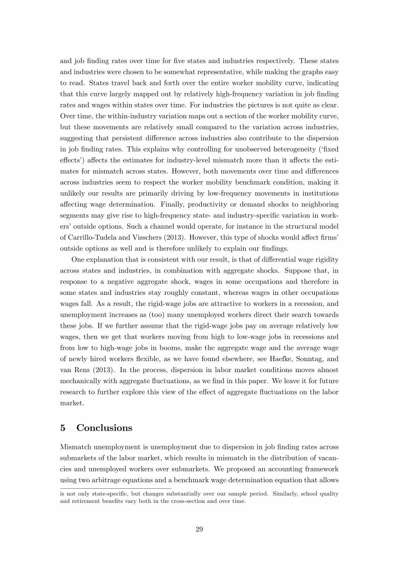
and job finding rates over time for five states and industries respectively. These states

and industries were chosen to be somewhat representative, while making the graphs easy

to read. States travel back and forth over the entire worker mobility curve, indicating

that this curve largely mapped out by relatively high-frequency variation in job finding

rates and wages within states over time. For industries the pictures is not quite as clear.

Over time, the within-industry variation maps out a section of the worker mobility curve,

but these movements are relatively small compared to the variation across industries,

suggesting that persistent difference across industries also contribute to the dispersion

in job finding rates. This explains why controlling for unobserved heterogeneity (‘fixed

effects’) affects the estimates for industry-level mismatch more than it affects the esti-

mates for mismatch across states. However, both movements over time and differences

across industries seem to respect the worker mobility benchmark condition, making it

unlikely our results are primarily driving by low-frequency movements in institutions

affecting wage determination. Finally, productivity or demand shocks to neighboring

segments may give rise to high-frequency state- and industry-specific variation in work-

ers’outside options. Such a channel would operate, for instance in the structural model

of Carrillo-Tudela and Visschers (2013). However, this type of shocks would affect firms’

outside options as well and is therefore unlikely to explain our findings.

One explanation that is consistent with our result, is that of differential wage rigidity

across states and industries, in combination with aggregate shocks. Suppose that, in

response to a negative aggregate shock, wages in some occupations and therefore in

some states and industries stay roughly constant, whereas wages in other occupations

wages fall. As a result, the rigid-wage jobs are attractive to workers in a recession, and

unemployment increases as (too) many unemployed workers direct their search towards

these jobs. If we further assume that the rigid-wage jobs pay on average relatively low

wages, then we get that workers moving from high to low-wage jobs in recessions and

from low to high-wage jobs in booms, make the aggregate wage and the average wage

of newly hired workers flexible, as we have found elsewhere, see Haefke, Sonntag, and

van Rens (2013). In the process, dispersion in labor market conditions moves almost

mechanically with aggregate fluctuations, as we find in this paper. We leave it for future

research to further explore this view of the effect of aggregate fluctuations on the labor

market.

5 Conclusions

Mismatch unemployment is unemployment due to dispersion in job finding rates across

submarkets of the labor market, which results in mismatch in the distribution of vacan-

cies and unemployed workers over submarkets. We proposed an accounting framework

using two arbitrage equations and a benchmark wage determination equation that allows

is not only state-specific, but changes substantially over our sample period. Similarly, school qualityand retirement benefits vary both in the cross-section and over time.

29

us to estimate mismatch unemployment and decompose it into its sources. Since this

framework takes data on the values of unemployment and vacancies rather than their

quantities as inputs, available data allowed us to present estimates for the 1979-2009

period, much further back in time that previous studies, in particular Sahin, Song, Topa,

and Violante (2014). This paper is also the first to report on the causes of mismatch.

We find that mismatch is an important reason for unemployment, in line with earlier

studies. The cyclical behavior of mismatch unemployment is very similar to that of

the overall unemployment rate. This finding is driven by the fact that dispersion in

labor market conditions across states and industries moves closely with the business

cycle. The unemployment that derives from this dispersion is as cyclical as the overall

unemployment rate and no more persistent. As a corollary, the nature of the increase in

unemployment in the Great Recession is no different from previous recessions, although

it is of course more severe.

The underlying frictions that cause mismatch to exist and persist are barriers to job

mobility (across industries) and deviations from surplus sharing in equal proportions

across industries and particularly across states. States with high wages tend to have

low profits. This implies that states and industries that are attractive to workers are

unattractive to firms and vice versa, generating dispersion in vacancy-unemployment

ratios and mismatch unemployment. Little to no mismatch derives from worker mobility

frictions. This finding is perhaps surprising in light of the debate on policies aimed at

increasing worker mobility.

30

References

Abowd, J. M. and A. Zellner (1985). Estimating gross labor-force flows. Journal ofBusiness and Economic Statistics 3 (3), 254—283.

Abraham, K. (1987). Help-wanted advertising, job vacancies, and unemployment.Brookings Papers on Economic Activity 18 (1), 207—248.

Abraham, K. G. and L. F. Katz (1986). Cyclical unemployment: Sectoral shifts oraggregate disturbances? Journal of Political Economy 94 (3), 507—22.

Alvarez, F. and R. Shimer (2011). Search and rest unemployment. Economet-rica 79 (1), 75—122.

Barnichon, R. and A. Figura (2010). What drives movements in the unemploymentrate? a decomposition of the Beveridge curve. Technical report.

Barnichon, R. and A. Figura (2013, October). Labor Market Heterogeneity and theAggregate Matching Function. Working Papers 727, Barcelona Graduate Schoolof Economics.

Berry, W. D., R. C. Fording, and R. L. Hanson (2000). An annual cost of living indexfor the American states, 1960-95. Journal of Politics 60 (2), 550—67.

Birchenall, J. A. (2011). A Competitive Theory of Mismatch. mimeo, University ofCalifornia at Santa Barbara.

Blanchard, O. and P. Diamond (1989). The Beveridge curve. Brookings Papers onEconomic Activity 20 (1), 1—76.

Blanchard, O. J. and L. F. Katz (1992). Regional evolutions. Brookings Papers onEconomic Activity 23 (1), 1—76.

Carrillo-Tudela, C. and L. Visschers (2013, January). Unemployment and EndogenousReallocation over the Business Cycle. IZA Discussion Papers 7124, Institute forthe Study of Labor (IZA).

Chang, B. (2011). A Search Theory of Sectoral Reallocation. Department of finance,investment and banking working papers, University of Wisconsin, Madison.

Coles, M. G., P. Jones, and E. Smith (2010). A picture of stock-flow unemploymentin the united kingdom. Macroeconomic Dynamics 14 (04), 427—453.

DeLong, B. (2010). The sad thing is that Narayana Kocherlakota was sup-posed to be the smart one among the Minnesota economists... Sep-tember 26, http://delong.typepad.com/sdj/2010/09/the-sad-thing-is-that-narayana-kocherlakota-was-supposed-to-be-the-smart-one-among-the-minnesota-economists.html.

Diamond, P. (1982). Aggregate demand management in search equilibrium. Journalof Political Economy 90 (5), 881—94.

Diamond, P. (2011). Unemployment, vacancies, wages. American Economic Re-view 101 (4), 1045—72.

Elsby, M. W. L., B. Hobijn, and A. Sahin (2010). The labor market in the GreatRecession. Brookings Papers on Economic Activity 41 (1), 1—69.

Estevão, M. M. and E. Tsounta (2011, May). Has the Great Recession Raised U.S.Structural Unemployment? IMF Working Papers 11/105, International MonetaryFund.

31

Frey, W. H. (2009). The Great American Migration Slowdown: Regional andMetropolitan Dimensions. Report, Brooking Institution.

Furlanetto, F. and N. Groshenny (2013, June). Mismatch shocks and unemploymentduring the Great Recession. Working Paper 2013/16, Norges Bank.

Groshen, E. L. and S. Potter (2003). Has structural change contributed to a joblessrecovery? Current Issues in Economics and Finance, Federal Reserve Bank ofNew York 9 (8), 1—48.

Haefke, C., M. Sonntag, and T. van Rens (2013). Wage rigidity and job creation.Journal of Monetary Economics 60 (8), 887—899.

Hagedorn, M. and I. Manovskii (2008). The cyclical behavior of equilibrium unem-ployment and vacancies revisited. American Economic Review 98 (4), 1692—1706.

Hall, R. E. (2009). Reconciling cyclical movements in the marginal value of time andthe marginal product of labor. Journal of Political Economy 117 (2), 281—323.

Harris, J. R. and M. P. Todaro (1970). Migration, unemployment and development:A two-sector analysis. The American Economic Review 60 (1), pp. 126—142.

Kambourov, G. and I. Manovskii (2008, 02). Rising Occupational And Industry Mobil-ity In The United States: 1968-97. International Economic Review 49 (1), 41—79.

Kaplan, G. and S. Schulhofer-Wohl (2011). A sharp drop in interstate migration? notreally. Technical report.

Katz, L. (2010). Long term unemployment in the Great Recession. Testimony for theJoint Economic Committee, U.S. Congress, April 29.

Kocherlakota, N. (2010). Inside the FOMC. Speech in Marquette, MI, on August 17as president of the Federal Reserve Bank of Minneapolis.

Krugman, P. (2010). Structure of excuses. September 27, New York Times.

Kudlyak, M. (2011). The cyclicality of the user cost of labor with search and matching.Technical report.

Lazear, E. P. and J. R. Spletzer (2012). The United States labor market: status quoor a new normal? Proceedings - Economic Policy Symposium - Jackson Hole,405—451.

Lilien, D. M. (1982). Sectoral shifts and cyclical unemployment. Journal of PoliticalEconomy 90 (4), 777—93.

Lipsey, R. G. (1965). Structural and deficient-demand unemployment reconsidered.In A. M. Ross (Ed.), Employment Policy and the Labor Market, pp. 210—255. UCBerkeley Press.

Lubik, T. A. (2013). The shifting and twisting Beveridge curve: an aggregate per-spective. Technical report.

Marinescu, I. and R. Rathelot (2014). Mismatch unemployment and the geography ofjob search. mimeo, University of Warwick.

Montgomery, J. D. (1991, February). Equilibrium Wage Dispersion and InterindustryWage Differentials. The Quarterly Journal of Economics 106 (1), 163—79.

Mortensen, D. T. (1982). Property rights and effi ciency in mating, racing, and relatedgames. American Economic Review 72 (5), 968—79.

Nagypál, E. and D. Mortensen (2007). More on unemployment and vacancy fluctua-tions. Review of Economic Dynamics 10 (3), 327—347.

32

New York Times (2014). A Fed Policy Maker, Changing His Mind, Urges More Stim-ulus. Technical report, http://nyti.ms/19XrUVw.

Padoa Schioppa, F. (1991). Mismatch and Labour Mobility. Cambridge UniversityPress.

Petrongolo, B. and C. A. Pissarides (2001). Looking into the black box: A survey ofthe matching function. Journal of Economic Literature 39 (2), 390—431.

Phelps, E. S. (1994). Structural Slumps. Harvard University Press.

Pissarides, C. A. (1985). Short-run equilibrium dynamics of unemployment vacancies,and real wages. American Economic Review 75 (4), 676—90.

Pissarides, C. A. (2000). Equilibrium Unemployment Theory (2nd ed.). Cambridge:MIT Press.

Roback, J. (1982). Wages, rents, and the quality of life. Journal of Political Econ-omy 90 (6), 1257—78.

Rosen, S. (1979). Wages-based indexes of urban quality of life. In P. Mieszkowskiand M. Straszheim (Eds.), Current Issues in Urban Economics. Johns HopkinsUniversity Press.

Sahin, A., J. Song, G. Topa, and G. L. Violante (2014). Mismatch unemployment.American Economic Review 104 (11), 3529—64.

Shimer, R. (2005). The cyclical behavior of equilibrium unemployment and vacancies.American Economic Review 95 (1), 25—49.

Shimer, R. (2007). Mismatch. American Economic Review 97 (4), 1074—1101.

Shimer, R. (2012). Reassessing the ins and outs of unemployment. Review of EconomicDynamics 15 (2), 127—148.

U.S. Department of Labor (2010). Significant provisions of state unemployment insur-ance laws, effective July 2010. Employment and Training Administration, Offi ceof Unemployment Insurance.

Wong, J. (2012, July). Aggregate Reallocation Shocks and the Dynamics of Occupa-tional Mobility and Wage Inequality. School of Economics Working Papers 2012-04, University of Adelaide, School of Economics.

33

Table 1Robustness Analysis

MMU Sources of MMUlevel cycle level cycle

Mismatch across states WM JM WD WM JM WDBaseline 2.3 3.4 6 0 93 15 1 83Elasticity matching function, µ = 0.5 1.6 2.4 8 5 88 20 10 70____, µ = 0.7 3.4 5.1 5 −9 104 11 −13 102Flow payoff unemployment, b = 0.4 2.3 3.4 6 0 93 15 1 83____, b = 0.9 2.3 3.4 6 0 93 15 1 83State-specific deflators 2.6 3.7 12 −2 89 17 1 82Mean-reversion payoffs, δy = 0.3 2.3 3.4 7 2 90 16 5 79____, δy = 0.5 2.3 3.4 8 3 89 16 6 77Mean-reversion turnover, δτ = 0.3 2.3 3.4 23 39 47 27 26 47____, δτ = 0.5 2.3 3.4 29 38 33 31 33 36Control for observed worker heterogeneity 2.0 3.1 10 1 89 16 5 79Control for unobserved heterogeneity 1.4 2.0 12 7 81 20 18 62

Mismatch across industries WM JM WD WM JM WDBaseline 2.1 1.2 −10 46 64 −2 113 −11Elasticity matching function, µ = 0.5 1.5 1.0 −13 57 56 1 103 −3____, µ = 0.7 3.0 1.6 −6 21 86 0 88 12Flow payoff unemployment, b = 0.4 2.1 1.2 −10 46 64 −2 113 −11____, b = 0.9 2.1 1.2 −10 46 64 −2 113 −11Mean-reversion payoffs, δy = 0.3 2.1 1.2 −2 36 67 6 89 5____, δy = 0.5 2.1 1.2 0 34 66 7 76 17Mean-reversion turnover, δτ = 0.3 2.1 1.2 11 61 28 18 114 −32____, δτ = 0.5 2.1 1.2 16 70 14 21 117 −38Control for observed worker heterogeneity 3.6 3.2 −6 39 67 0 43 57Control for unobserved heterogeneity 1.1 0.3 8 14 79 30 31 39

The contributions of mismatch to the level and cyclicality of unemployment is estimatedusing the following regression, uMM

t = β0u+ β1 (ut − u), where β0 = uMM/u measuresthe contribution to the level and β1

(= ∆uMM/∆u

)the contribution to fluctuations

in unemployment. Similarly, the contributions of the various sources to mismatch areestimated using uXXt = βXX0 uMM + βXX1

(uMMt − uMM

), where XX stands for the

source, i.e. XX ∈ {WM,JM,WD}.

34

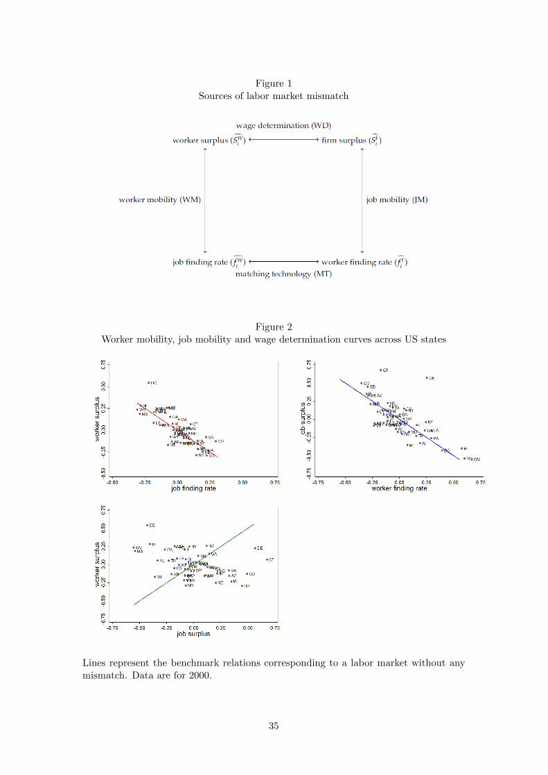
Figure 1Sources of labor market mismatch

Figure 2Worker mobility, job mobility and wage determination curves across US states

Lines represent the benchmark relations corresponding to a labor market without anymismatch. Data are for 2000.

35

Figure 3Worker mobility, job mobility and wage determination curves across industries

Lines represent the benchmark relations corresponding to a labor market without anymismatch. Data are for 2000.

36

Figure 4Cyclicality of mismatch unemployment across US states

Unemployment due to mismatch across US states, calculated as explained in 2.2. Thedashed line shows the actual unemployment rate for comparison (right-hand side axis).

Figure 5Cyclicality of mismatch unemployment across industries

Unemployment due to mismatch across industries, calculated as explained in 2.2. Thedashed line shows the actual unemployment rate for comparison (right-hand side axis).

37

Figure 6Sources of labor market mismatch across US states

The solid line is our baseline estimate for mismatch unemployment, calculated as ex-plained in 2.2. The other lines show the contribution of worker mobility costs (WM),job mobility costs (JM) and wage setting frictions (WD) to mismatch, see 2.3.

Figure 7Sources of labor market mismatch across industries

The solid line is our baseline estimate for mismatch unemployment, calculated as ex-plained in 2.2. The other lines show the contribution of worker mobility costs (WM),job mobility costs (JM) and wage setting frictions (WD) to mismatch, see 2.3.

38

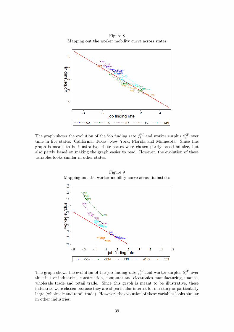
Figure 8Mapping out the worker mobility curve across states

The graph shows the evolution of the job finding rate fWi and worker surplus SWi overtime in five states: California, Texas, New York, Florida and Minnesota. Since thisgraph is meant to be illustrative, these states were chosen partly based on size, butalso partly based on making the graph easier to read. However, the evolution of thesevariables looks similar in other states.

Figure 9Mapping out the worker mobility curve across industries

The graph shows the evolution of the job finding rate fWi and worker surplus SWi overtime in five industries: construction, computer and electronics manufacturing, finance,wholesale trade and retail trade. Since this graph is meant to be illustrative, theseindustries were chosen because they are of particular interest for our story or particularlylarge (wholesale and retail trade). However, the evolution of these variables looks similarin other industries.

39