Accounting for Intermediates:Production Sharing and Trade in Value Added∗

Robert C. Johnson†

Dartmouth CollegeGuillermo Noguera‡

Columbia Business School

First Draft: July 2008This Draft: May 2011

Abstract

We combine input-output and bilateral trade data to compute the value added content ofbilateral trade. The ratio of value added to gross exports (VAX ratio) is a measure of the in-tensity of production sharing. Across countries, export composition drives VAX ratios, withexporters of Manufactures having lower ratios. Across sectors, the VAX ratio for Manufac-tures is low relative to Services, primarily because Services are used as an intermediate toproduce manufacturing exports. Across bilateral partners, VAX ratios vary widely and containinformation on both bilateral and triangular production chains. We document specifically thatbilateral production linkages, not variation in the composition of exports, drives variation inbilateral VAX ratios. Finally, bilateral imbalances measured in value added differ from grosstrade imbalances. Most prominently, the U.S.-China imbalance in 2004 is 30-40% smallerwhen measured in value added.

∗We thank Rudolfs Bems, Judith Dean, Stefania Garetto, Pierre-Olivier Gourinchas, Russell Hillberry, David Hum-mels, Brent Neiman, Nina Pavcnik, Esteban Rossi-Hansberg, Zhi Wang, and Kei-Mu Yi for helpful conversations, aswell as participants in presentations at the Federal Reserve Board, Hamilton College, Harvard University, the Interna-tional Monetary Fund, the Philadelphia Federal Reserve, Princeton University, the U.S. International Trade Commis-sion, University of California (Berkeley), University of Cape Town, Wesleyan University, the 2009 FREIT EmpiricalInvestigations in International Trade conference, and the 2010 AEA Meetings. Noguera gratefully acknowledgesfinancial support from UC Berkeley’s Institute for Business and Economic Research.†Corresponding Author. Department of Economics, Dartmouth College, Hanover, NH 03755, USA. E-mail:

robert.c.johnson@dartmouth.edu. Telephone: +1-847-532-0443.‡Columbia Business School, 6-0 Uris Hall, 3022 Broadway, New York, NY 10027, USA. E-mail:

gn2195@columbia.edu.

1

Trade in intermediate inputs accounts for as much as two thirds of international trade. By

linking production processes across borders, this input trade creates two distinct measurement

challenges. First, conventional gross trade statistics tally the gross value of goods at each border

crossing, rather than the net value added between border crossings. This well-known “double-

counting” problem means that conventional data overstate the domestic (value added) content of

exports. Second, multi-country production networks imply that intermediate goods can travel to

their final destination by an indirect route. For example, if Japanese intermediates are assembled

in China into final goods exported to the U.S., then Chinese bilateral gross exports embody third

party (Japanese) content. Together, “double-counting” and multi-country production chains imply

that there is a hidden structure of trade in value added underlying gross trade flows.

In this paper, we compute and analyze the value added content of trade. To do so, we require a

global bilateral input-output table that describes how particular sectors in each destination country

purchase intermediates from both home and individual foreign sources, as well as how each country

sources final goods. Because these bilateral final and intermediate goods linkages are not directly

observed in standard trade and national accounts data sources, we construct a synthetic table by

combining input-output tables and bilateral trade data for many countries. Using this table, we

split each country’s gross output according to the destination in which it is ultimately absorbed in

final demand. We then use value added to output ratios from the source country to compute the

value added associated with the implicit output transfer to each destination. The end result is a

data set of “value added exports” that describes the destination where the value added produced in

each source country is absorbed.

These data on the value added content of trade have many potential uses. Most directly, we

compare them to gross bilateral trade flows to quantify the scope of production sharing. This ap-

proach to measuring production sharing yields comparable figures for many countries and sectors

and respects the multilateral structure of production sharing. Further, because we use the national

accounts definition of intermediates, our measures are easily translated into models.1 This is im-

1This contrasts with alternative approaches, such as using data on trade in parts and components (e.g., Yeats (2001))or trade between multinational parents and affiliates (e.g., Hanson, Mataloni, and Slaughter (2005)).

2

portant because the value added content of trade is a key theoretical object and calibration target in

many trade and macroeconomic models. For example, value added exports can be used to calibrate

“openness” and bilateral exposure to foreign shocks in international business cycle research.2 For

trade research, value added flows could be used to calibrate gravity-style trade models to allow

for differences in trade patterns for final and intermediate goods.3 They could also be employed

to calibrate many-country models of multi-stage production and vertical specialization, as in Yi

(2003, 2010). And these applications only scratch the surface.

Our approach to measuring the value added content of trade draws upon a venerable literature

on input-output accounting in models with multiple regions.4 It is also intimately related to recent

efforts to measure the factor content of trade with traded intermediates. Specifically, Trefler and

Zhu (2010) develop a multi-country input-output framework to define a Vanek-consistent measure

of the factor content of multilateral net exports.5 We elaborate on the relationship between com-

puting value added and factor contents in our discussion of the calculation procedure. Belke and

Wang (2006) and Daudin, Rifflart, and Schweisguth (forthcoming) also develop value added trade

computations along the lines of those used in this paper, though our exposition and analysis differ

considerably.6

Our work is also related to an active literature on measuring vertical specialization and the

domestic content of exports.7 Aggregating across sectors and export destinations for each source

country, the ratio of value added to gross exports can be interpreted as a metric of the domestic

content of exports.8 Our domestic content metric generalizes the work by Hummels, Ishii, and Yi

(2001). Hummels et al. compute the value added content of exports under the restrictive assump-

2See Bems, Johnson, and Yi (2010) for elaboration of this argument.3See Noguera (2011) for an analysis of estimated trade elasticities in gravity models with and without intermediate

goods.4See Isard (1951), Moses (1955), Moses (1960), or Miller (1966).5Reimer (2006) exposits an equivalent approach in a two country case.6Daudin, Rifflart, and Schweisguth study the role of vertical specialization in generating regionalization in trade

patterns, while Belke and Wang focus on measuring aggregate economic openness. See also more recent work byPowers, Wang, and Wei (2009) on splitting up the value chain within Asia.

7See NRC (2006) for the U.S. See Dean, Fung, and Wang (2007), Chen, Cheng, Fung, and Lau (2008), andKoopman, Wang, and Wei (2008) for China. See Hummels, Ishii, and Yi (2001) and Miroudot and Ragoussis (2009)for changes in domestic content over time for mainly OECD countries.

8Bilateral or sector level ratios of value added to exports do not have this domestic content interpretation.

3

tion that a country’s exports (whether composed of final versus intermediate goods) are entirely

absorbed in final demand abroad. That is, it rules out scenarios in which a country exports in-

termediates that are used to produce final goods absorbed at home. By using input-output data

for source and destination countries simultaneously, we are able to relax this assumption. While

this generalization results in only minor adjustments in aggregate domestic content measurements

in our data, we demonstrate that relaxing this assumption is critically important for generating

accurate bilateral value added flows.

Turning to our empirical results, we find that the ratio of value added to gross exports (VAX ra-

tio) varies substantially across countries and sectors. Across sectors, we show that VAX ratios are

substantially higher in Agriculture, Natural Resources, and Services than in Manufactures. This

is mostly due to the fact that the manufacturing sector purchases inputs from non-manufacturing

sectors, and therefore contains value added generated in those sectors. Across countries, the com-

position of trade drives aggregate VAX ratios, with countries that export Manufactures having

lower aggregate VAX ratios. Aggregate VAX ratios do not covary strongly with income per capita,

however, due to two offsetting effects. While richer countries tend to export Manufactures, which

lowers their aggregate VAX ratios, they also export at higher VAX ratios within the manufacturing

sector.9

Moving from aggregate to bilateral data, VAX ratios differ widely across partners for individual

countries. For example, U.S. exports to Canada are about 40% smaller measured in value added

terms than gross terms, whereas U.S. exports to France are essentially identical in gross and value

added terms. These gaps arise for two main reasons. First, bilateral (“back-and-forth”) production

sharing implies that value added trade is scaled down relative to gross trade. And these scaling

factors differ greatly across bilateral partners. Second, multilateral (“triangular”) production shar-

ing gives rise to indirect trade that occurs via countries that process intermediate goods. For some

country pairs, bilateral VAX ratios are larger than one, as bilateral value added exports exceeds

gross exports.

9VAX ratios within Manufactures are correlated with income because richer countries tend to export in sub-sectorswith relatively high VAX ratios.

4

These adjustments imply that bilateral trade imbalances often differ in value added and gross

terms. For example, the U.S.-China imbalance is approximately 30-40% smaller when measured

on a value added basis, while the U.S.-Japan imbalance is approximately 33% higher. These

adjustments point to the importance of triangular production chains within Asia.

To illustrate the mechanisms at work in generating these results, we present two decomposi-

tions. In the first decomposition, we show that most of the variation in bilateral value added to

export ratios arises due to production sharing, not variation in the composition of goods exported

to different destinations. The second decomposition splits bilateral exports according to whether

they are absorbed in the destination, embedded as intermediates in goods that are reflected back to

the source country, or redirected to third countries embedded as intermediates in goods ultimately

consumed there. Variation in the degree of absorption, reflection, and redirection across partners

is an important driver of variation in bilateral value added to export ratios.

The rest of the paper is structured as follows. Section 1 presents the general accounting frame-

work, defines our value added trade measures, and discusses the interpretation of value added

to export ratios. Section 2 describes the data sources and assumptions we use to implement the

accounting exercise. Section 3 presents our empirical results and Section 4 concludes.

1 The Value Added Content of Trade

In this section, we introduce the accounting framework and demonstrate how intermediate goods

trade generates differences between gross and value added trade flows. We begin the section by

presenting a general formulation of the framework with many goods and countries that we use in

the calculations below. To aid intuition, we then exposit several results in stripped-down versions

of this general framework. Results from these simple models carry over to the general model.

We close by discussing the relationship between our framework and two related lines of work on

regional input-output linkages and measurement of the factor content of trade.

5

1.1 The Value Added Content of Trade

Assume there are S sectors andN countries. Each country produces a single differentiated tradable

good within each sector, and we define the quantity of output produced in sector s of country i to

be qi(s). This good is produced by combining local factor inputs with domestic and imported

intermediate goods. It is then either used to satisfy final demand (equivalently, “consumed”) or

used as an intermediate input in production.

The key feature of the global input-output framework is that it tracks bilateral shipments of this

output for final and intermediate use separately. To track these flows requires four dimensional

notation denoting source and destination country, as well as source and destination sectors for

shipments of intermediates. Let the quantity of final goods from sector s in country i absorbed in

destination j be qcij(s) and the quantity of intermediates from sector s in country i used to produce

output in sector t in country j be qmij (s, t).

The global input-output framework organizes these flows via market clearing conditions. Mar-

kets clear in quantities: qi(s) =∑

j qcij(s) +

∑j

∑t q

mij (s, t). If we evaluate these quantity flows

at a common price, say pi(s), then we can rewrite the market clearing condition in value terms as:

yi(s) =∑

jcij(s) +

∑j

∑tmij(s, t), (1)

where yi(s) ≡ pi(s)qi(s), cij(s) ≡ pi(s)qcij(s), and mij(s, t) ≡ pi(s)q

mij (s, t) are the value of pro-

duction, final demand, and intermediate goods shipments. Gross bilateral exports, denoted xij(s),

include goods destined for both final and intermediate use abroad: xij(s) = cij(s) +∑

tmij(s, t).

Then (1) equivalently says that output is divided between domestic final use, domestic intermediate

use, and gross exports.

To express market clearing conditions for many countries and sectors in a compact form, we

define a series of matrices and vectors. Collect the total value of production in each sector in the

S × 1 vector yi and allocate this output to final and intermediate use. Denote country i’s final

demand for its own goods by S × 1 vector cii and shipments of final goods from i to country j by

6

the S×1 vector cij . Further, denote use of intermediate inputs from i by country j by Aijyj , where

Aij is an S × S input-output matrix with elements Aij(s, t) = mij(s, t)/yj(t). A typical element

describes, for example, the value of steel (s = steel) imported by Canada (j = Canada) from the

U.S. (i = U.S.) used in the production of automobiles (t = autos) as a share of total output of autos

in Canada. Gross exports from i to j (i 6= j) are then xij = cij + Aijyj .

With this notation in hand, we collect information on intermediate goods sourcing and final

goods flows in vector/matrix form:

A ≡

A11 A12 . . . A1N

A21 A22 · · · A2N

...... . . . ...

AN1 AN2 . . . ANN

, y ≡

y1

y2...

yN

, cj ≡

c1j

c2j...

cNj

.

Then, we write the S ×N goods market clearing conditions as:

y = Ay +∑

jcj. (2)

This is the classic representation of an input-output system, where total output is split between in-

termediate and final use. Whereas a typical input-output system focuses on sectoral linkages within

a single economy, this system is expanded to trace intermediate goods linkages across countries

and sectors. We therefore refer to A as the global bilateral input-output matrix.

Using this system, we can write output as:

y =∑

j(I − A)−1cj. (3)

To interpret this expression, (I − A)−1 is the “Leontief inverse” of the input-output matrix. The

Leontief inverse can be expressed as a geometric series: (I − A)−1 =∑∞

k=0Ak. Multiplying by

the final demand vector, the zero-order term cj is the direct output absorbed as final goods, the

first-order term [I + A]cj is the direct output absorbed plus the intermediates used to produce that

7

output, the second-order term [I+A+A2]cj includes the additional intermediates used to produce

the first round of intermediates (Acj), and the sequence continues as such. Therefore, (I −A)−1cj

is the vector of output used both directly and indirectly to produce final goods absorbed in country

j.

Equation (3) thus decomposes output from each source country i into the amount of output

from the source used to produce final goods absorbed in country j. To make this explicit, we

define:

y1j

y2j...

yNj

≡ (I − A)−1cj, (4)

where yij is the S × 1 vector of output from i used to produce final goods absorbed in j.

These output transfers are conceptually distinct from gross exports. Gross exports xij(s) are

directly observed as a bilateral shipment from sector s in country i to country j. In contrast,

bilateral output transfers are not directly observed, but rather constructed using information on the

global input requirements for final goods absorbed in each country. Importantly, as inputs from a

particular country and sector travel through the production chain, they may be embodied in final

goods of any sector or country. For example, inputs exported from country i to country j may be

embedded in country j final goods that are absorbed in a third country k, or inputs produced by

sector s may be embodied in final goods from sector t. These possibilities give rise to important

differences in the structure of bilateral output transfers versus bilateral trade.

To calculate the value added associated with these implicit output transfers, define the ratio of

value added to output for each sector within country i, as ri(t) = 1−∑

j

∑sAji(s, t). This value

added ratio, expressed here as one minus the share of domestic plus imported intermediates in total

output, is equal to payments to domestic factors as a share of gross output. Put differently, this is

ratio of GDP to gross output at the sector level.

With this notation in hand, we can now define value added exports and the value added to

8

export ratio, “VAX ratio”, as a measure of the value added content of trade.

Definition 1 (Value Added Exports). The total value added produced in sector s in source country

i and absorbed in destination country j is vaij(s) = ri(s)yij(s). Total value added produced in i

and absorbed in j is then vaij =∑

s vaij(s).

Definition 2 (VAX Ratio). The sector-level bilateral value added to export ratio is given by

vaij(s)/xij(s). The aggregate bilateral value added to export ratio is vaij/ιxij , where ι is a 1× S

vector of ones.

1.2 Discussion

We turn to special cases to interpret value added trade flows and the value added content of trade.

We use a two country model to develop intuition for the value added content of trade calculations

and link our analysis to previous work on the domestic content of exports (equivalently, vertical

specialization) by Hummels, Ishii, and Yi (2001). We then use a stylized three country model to

demonstrate how the framework tracks value added through the multi-country production chain,

even if that value added travels to its final destination via third countries. We also discuss the

interpretation of VAX ratios in multi-sector models. We conclude by setting our framework in

context of related literature on regional input-output linkages and the measurement of the factor

content of trade.

1.2.1 Two Countries, One Sector Per Country

Suppose that there are now only two countries, and each country produces a single differentiated

aggregate good. Then the analog to the output decomposition (3) is:

y1y2

=

I −α11 α12

α21 α22

−1c11

c21

+

I −α11 α12

α21 α22

−1c12

c22

. (5)

This system describes how the gross output of each country is embodied in final consumption

9

in each of the two countries. To unpack this result, we solve for the breakdown of country 1’s

production:

y1 = y11 + y12

with y11 = M1

(c11 +

α12

1− α22

c21

)and y12 = M1

(α12

1− α22

c22 + c12

),

(6)

whereM1 ≡(

1− α11 − α12α21

1−α22

)−1≥ 1 is an intermediate goods multiplier that describes the total

amount of gross output from country 1 required to produce one unit of country 1’s net output.10

The first term (y11) is the total amount of country 1’s output that is required to produce final

goods absorbed in country 1. This term includes both output dedicated to satisfy country 1’s

demand for its own final goods (M1c11), as well as output needed to satisfy country 1’s demand

for country 2 final goods(M1

α12

1−α22c21

).11 The second term (y12) has a similar interpretation

in terms of country 2’s demand.12 Because (6) geographically decomposes country 1’s output,

we can translate this into a decomposition of value added: va1 = va11 + va12, where vaij =

[1− α11 − α21]yij is value added generated by country i that is absorbed in country j.

There are four output concepts underlying flows from country 1 to country 2: (1) final goods

c12, (2) gross exports x12, (3) implicit output transfers y12, and (4) value added exports va12. We

pause here to clarify the relationship between them. To begin, note that x12 = c12 + α12y2, so

c12 ≤ x12 when there are exported intermediates. Further, using the output decomposition for

country 2 (y2 = y22 + y21), we decompose gross exports as: x12 = α12y21 + (c12 + α12y22).

Multiplying both sides of the expression by (1−α11)−1 then translates exports into the gross output

required to produce them.13 It is straightforward to show that y12 = (1 − α11)−1(c12 + α12y22).

10This multiplier is greater than one because output is “used up” in the production process. Without exportedintermediates (α12 = 0), this multiplier would be (1− α11)

−1. The additional term reflects the fact that intermediategoods sourced from country 2 contain output produced by country 1.

11To export final goods c21 requires producing (1 − α22)−1c21 units of country 2 output, which itself requires

α12(1 − α22)−1c21 units of country 1’s output as intermediates. To produce this country 1 output requires M1 times

α12(1− α22)−1c21 units of country 1’s output overall, because some output is used up in the production process.

12To highlight how the output decomposition depends on cross-border intermediate linkages, note that if α12 = 0the output decomposition would be: y11 = (1 − α11)

−1c11 and y12 = (1 − α11)−1c12. In this counter-factual case,

output of country 1 is only used to produce final goods originating in country 1.13This follows from manipulation of the market clearing condition for country 1: y1 = (1− α11)

−1(c11 + x12).

10

Therefore, y12 = (1 − α11)−1x12 − (1 − α11)

−1α12y21. So the implicit output transferred from

country 1 to country 2 is equal to the gross output required to produce exports minus the gross

output that is reflected back embedded in country 2 goods that are absorbed by country 1.14 Finally,

we note that va12 ≤ y12, because the value added to output ratio is bounded above by one.

To directly compare value added exports to gross exports, we compute the VAX ratio:

va12x12

=(1− α11 − α21)y12

x12

=1− α11 − α21

1− α11

(x12 − α12y21

x12

),

(7)

where the second line follows from the discussion in the previous paragraph. The difference x12−

α12y21 is exports less reflected intermediates, or equivalently the portion of exports genuinely

consumed abroad. The VAX ratio will always be less than one, so value added exports are scaled

down relative to gross exports.

The VAX ratio for a country can be thought of as a metric of the “domestic content of exports.”

Indeed, it is closely related to previous approaches to measuring domestic content in the literature.

To see this, note that the VAX ratio has two components. The first component, 1−α11−α21

1−α11, is equiv-

alent to a metric of domestic content developed in Hummels, Ishii, and Yi (2001).15 This metric

captures the value added associated with the gross output needed to produce exports as a fraction

of total exports. The Hummels-Ishii-Yi metric is equal to the VAX ratio only when country 2 does

not use imported intermediates (α12 = 0), and therefore country 1 exports final goods alone.16 In

contrast, with two-way trade in intermediates the Hummels-Ishii-Yi metric overstates the amount

of domestic value added that is generated per unit of exports.17 The second component of the

14Note that if α12 = 0, then y12 = (1 − α11)−1x12, so the gross output required to produce exports equals the

actual amount of output transferred from country 1 to country 2.15Hummels et al. focus their discussion on measuring vertical specialization or the “import content of exports,”

which is given by α21(1 − α11)−1. Domestic content is then one minus the import content of exports. Though we

discuss these concepts here in a scalar case, they generalize in a straightforward way to models with many sectors.16The condition α12 = 0 is necessary and sufficient for equality between the two metrics when there is one aggregate

sector, except in pathological cases. With more than one sector, restricting country 1 to export only final goods(α12(s, t) = 0 ∀ s, t) is sufficient, but not necessary.

17Footnote 18 in Trefler and Zhu (2010) provide a related discussion of how the factor content of trade differsdepending on whether one assumes intermediates are traded or not.

11

VAX ratio allows some exports to be dedicated to producing goods that are ultimately consumed

at home. That is, it allows for a portion of exports to be reflected back to the source rather than

absorbed abroad.

1.2.2 Three Countries, One Sector Per Country

While the two country framework illustrates the basic discrepancy between value added and gross

trade flows, additional insights emerge as one introduces a third country to the mix. We focus on a

special, algebraically straightforward case that illustrates how the accounting framework tracks the

final destination at which value added by a given country is consumed even if this value circulates

through a multi-country production chain en route to its final destination. We construct the special

case to approximate a stylized account of production chains between the U.S. and Asia.18

Let country 1 be the U.S., country 2 be China, and country 3 be Japan. Further, assume that

China imports intermediates from the U.S. and Japan and exports only final consumption goods

only to the U.S. For simplicity, we assume that the U.S. and Japan do not export any final goods

and only export intermediates to China. This configuration of production can be represented as:

y1

y2

y3

=

α11 α12 0

0 α22 0

0 α32 α33

y1

y2

y3

+

c11

c22 + c21

c33

. (8)

18This example was inspired by Linden, Kraemer, and Dedrick (2007), who trace the iPod production chain. TheiPod combines U.S. intellectual property from Apple with a Japanese display and disk drive, which is manufacturedin China. These components are assembled in China and the iPod is shipped to the U.S.

12

This then can be solved to yield the following three-equation system:

y1 =1

1− α11

c11 +α12

(1− α11)(1− α22)c21︸ ︷︷ ︸

y11

+α12

(1− α11)(1− α22)c22︸ ︷︷ ︸

y12

y2 =1

1− α22

c21︸ ︷︷ ︸y21

+1

1− α22

c22︸ ︷︷ ︸y22

y3 =α32

(1− α33)(1− α22)c21︸ ︷︷ ︸

y31

+α32

(1− α33)(1− α22)c22︸ ︷︷ ︸

y32

+1

1− α33

c33︸ ︷︷ ︸y33

.

(9)

This system provides the implicit output transfers needed to calculate value added flows.

Two points are interesting to note. First, as in the two-country case above, U.S. demand for

U.S. output has both a direct component 1(1−α11)

c11, and an indirect component α12

(1−α11)(1−α22)c21

that accounts for the fact that U.S. imports of final goods from China include embedded U.S.

content. Thus, a larger share of U.S. output is ultimately absorbed at home than bilateral trade

statistics would indicate. Correspondingly, Chinese bilateral exports overstate the true Chinese

content shipped to the U.S. due to bilateral U.S.-China production sharing.

The second point is that, although Japan does not export directly to the U.S., the U.S. does

import Japanese content embedded in Chinese exports to the U.S. This effect is the result of multi-

country production chains, and was absent in the two country case analyzed above. In the equation

for Japan (country 3), this effect appears as α32

(1−α33)(1−α22)c21.

Because Chinese exports to the U.S. contain both U.S. and Japanese content, the bilateral VAX

ratio of China-U.S. trade is:

va21x21

= 1−(va31 + α12y21

x21

)< 1. (10)

This illustrates that the bilateral VAX ratio removes both the Japanese value added (va31) and U.S.

intermediate goods (α12y21) from Chinese exports to the U.S.19 Turning to Japan, it has positive

19U.S. imports from China contain U.S. content because the U.S. exports intermediates to China and imports finalgoods from China. Thus, U.S. intermediates are reflected back to the US and constitute a portion of the value added

13

value added exports to the U.S. and zero direct bilateral exports. Therefore, the bilateral VAX ratio

for Japan-U.S. trade is undefined, or practically infinite for small bilateral exports. This extreme

ratio illustrates another general lesson. Though the aggregate VAX ratio is bounded by one for

each country, bilateral VAX ratios may be greater than one when an exporter sends intermediates

abroad to be processed and delivered to a third country. Thus, bilateral VAX ratios pick up the

influence of both bilateral and multilateral production sharing relationships.

When bilateral VAX ratios vary across partners, bilateral value added balances do not equal

bilateral trade imbalances. To illustrate this, we define tb12 ≡ x12 − x21 and vab12 ≡ va12 −

va21 to be bilateral U.S.-China trade and value added balances. In this special case, where the

configuration of production is given by (8), these balances are related as follows:

tb12 + α32y21 = vab12. (11)

That is, tb12 < vab12. So assuming the U.S. runs a trade deficit with China in this example, then

it will run a smaller deficit with China in value added terms due to the fact that Chinese bilateral

trade contains Japanese content (α32y21). As a corollary, the U.S.’s bilateral balance with Japan

will be distorted in the opposite direction.

To generalize this result, we can write any given bilateral value added balance as:

vabij =vaijxij

xij −vajixji

xji

=1

2(xij + xji)

[vaijxij− vaji

xji

]+

1

2

(vaijxij

+vajixji

)[xij − xji] .

(12)

The first term adjusts the value added balance due to differences in VAX ratios between exports

and imports. When the VAX ratio for exports is high relative to imports, the value added balance is

naturally pushed in a positive direction. Note here that this is true even if gross trade is balanced.

The second term adjusts the value added balance based on the average level of VAX ratios. Starting

from an initial imbalance, the value added balance is scaled up or down relative to the trade balance,

that the U.S. purchases from itself.

14

depending on whether VAX ratios are greater than or less than one (on average). So differences

in VAX ratios between partners within a bilateral relationship and the absolute level of the VAX

ratios between partners both influence the size of the adjustment in converting gross imbalances to

value added terms.

1.2.3 Two Countries, Many Sectors

The interpretation of aggregate value added exports and VAX ratios developed in the one-sector

examples in previous sections carries over to the many country, multi-sector framework. One

important distinction between the one-sector and multi-sector frameworks is that VAX ratio at the

sector level cannot be interpreted as the domestic content of exports. To explain its interpretation,

we turn to an example with two countries and many sectors.20

With two countries (i, j = {1, 2}) and many sectors, the VAX ratio for sector s in country 1

can be written as: va12(s)x12(s)

= r1(s)y12(s)x12(s)

. Then the sectoral VAX ratio depends on the value added to

output ratio within a given sector (r1(s)) and the ratio of gross output produced in a sector that is

absorbed abroad (y12(s)) to gross exports from that sector (x12(s)). The role of the value added to

output ratio is straightforward: all else equal, sectors with low value added to output ratios (e.g.,

manufacturing) will have low VAX ratios relative to other sectors.

The role of differences in y12(s) versus x12(s) across sectors is more subtle. To sort this out,

we note that we can link y12 and the export vector x12 as in Section 1.2.1. Specifically, x12 =

(I − A11)y12 + A12y21. Rearranging this expression yields: y12 = (I − A11)−1 [x12 − A12y21].

This is the many sector, matrix analog to computations embedded in Equation 7, wherein y12 is the

gross output needed to produce exports less reflected intermediates. This decomposition points to

two ways in y12 could differ from x12.

First, suppose that A12y21 is a vector of zeros, so that exports are 100% absorbed abroad.21

20The many country version of the framework can always be collapsed to an equivalent two country framework, inwhich input-output linkages among countries in the rest of the world are subsumed into the “domestic” input-outputstructure of the rest-of-the-world composite.

21If A12 is matrix of zeros, so that country 1 exports only final goods, this obviously holds. This can also hold forcases in which elements of A12 are positive, so long as the corresponding elements y21 are zero. For example, country1 could export intermediates to country 2, so long as the sector purchasing those intermediates only produces output

15

This implies: y12 = (I − A11)−1x12. All that remains here separating exports and gross output for

individual sectors is the domestic input-output structure. Generically, y12(s) 6= x12, so variation in

this ratio across sectors influences sector-level value added.

One important implication of this is that the sectoral VAX ratio captures information on how

individual sectors engage in trade. For example, consider a situation in which producers in one

sector sell intermediates to purchasers in another sector, who in turn produce goods for export.22

In this case, the intermediate goods suppliers engage in trade indirectly. Hence, we observe no

direct exports from the intermediate goods supplier, but do observe value added exports because

value added from that sector is embedded in the purchaser’s goods. Thus, value added exports from

a particular sector may be physically embodied in goods exported from that sector or embodied in

exports of other sectors. High ratios of value added exports to gross trade (possibly above one) at

the sector level are evidence of indirect participation in trade. Low ratios instead indicate that a

given sector’s gross exports embody value added produced outside that sector.

Second, suppose now that A12 is not composed of zeros, but rather that country 1 exports

intermediates to country that are used to produce goods that are absorbed in country 1, captured by

the term A12y21 > 0. In this case, the sectoral VAX ratio is influenced by how individual sectors

fit into cross-border production chains. For example, if we shut down all domestic input-output

linkages, setting A11 to zero, then y12 = x12 − A12y21. Then the sectoral VAX ratio depends on

the sector’s connection to foreign production chains. Specifically, the VAX ratio will be depend on

what share of output is absorbed abroad versus used to produce foreign goods that are ultimately

absorbed at home. If exports are largely absorbed abroad (i.e., y12(s)/x12(s) ≈ 1), one would see

a relatively high VAX ratio.

Though these influences are difficult to separate empirically in general cases, we discuss evi-

dence below that sheds light on the relative importance of these channels.

for consumption in country 2.22For example, the “raw milk” sector in our data has near zero exports, but raw milk is sold to the “dairy products”

sector, which does export. With two sectors, where 1 is the dairy products and 2 is the milk sector, this could berepresented as an A11 matrix with one non-zero element α11(2, 1) and export vector with x12(1) > 0 and x12(2) = 0.This structure implies y12(1)/x12(1) = 1 and y12(2)/x12(2) =∞

16

1.2.4 Regional Input-Output Models and the Factor Content of Trade

The framework above is intimately related to two strands of literature in regional science and trade.

First, we draw on an extensive literature on regional input-output models. These models, out-

lined in seminal work by Isard (1951), Moses (1955), Moses (1960), and Miller (1966), provide

frameworks for analyzing linkages across regions within countries that can be extended across

borders (as above). Among this literature, Moses (1955) is the closest antecedent, as he uses

proportionality assumptions to allocate inputs purchased from other regions, as we do, to build a

multi-region model of the U.S.23 One shortcoming of this line of work is that it typically assumes

that the regional system is ‘open’ vis-a-vis the rest-of-the-world, in the sense that shipments to

regions not included in the model are entirely absorbed there. This assumption is a multi-region

analog of the assumptions under which the Hummels-Ishii-Yi (2001) domestic content calculation

is equal to the value added content of trade.24

Second, the value added framework above shares a common structure with a recent parallel

literature on measuring the factor content of trade. Reimer (2006) and Trefler and Zhu (2010) both

outline procedures to compute the net factor content of trade when inputs are traded, and use these

factor content measures to study the Vanek prediction. To draw out the similarities, note that one

can think of computing both factor contents and value added contents using a two step procedure.

First, one needs to compute the output transfers, specified above, that indicate how much output

from each source country and sector are absorbed in final demand in a given destination. Second,

one needs to use source country information on either factor contents (e.g., quantities of factors

used to produce one dollar of output) or value added to output ratios to compute the factors or

value added that is implicitly being traded.25

23Isard (1951) suggests this technique as well, but does not pursue an empirical application himself.24Powers, Wang, and Wei (2009) work with a model of this type for Asia.25Let us trace out the calculation explicitly. Trefler and Zhu define Ti to be a (NS × 1) vector of trade flows

arranged as follows: Ti = [· · · ,−x′i−1,i, x′i,−x′i+1,i, · · · ]′, where xi =∑

j 6=i xij is a (S × 1) vector of total exportsfrom country i to the rest of the world and xj,i is a (S × 1) vector of bilateral trade flows from j 6= i to i. Further,they define B to be a F × SN matrix of factor requirements for each good: B ≡ [B1, · · · , Bi, · · · , BN ], where Bi isthe F × S matrix of factor requirements for country i, with F denoting the number of factors. The factor content oftrade for country i is then: B(I − A)−1Ti. To link this to our framework, we note that the calculation (I − A)−1Tireturns a vector of (signed) output transfers. In particular, (I − A)−1Ti = [· · · ,−y′i−1,i, y′xi,−y′i+1,i, · · · ]′, where

17

Despite this similarity in the underlying structure of value added and factor content calcula-

tions, we emphasize that there are important conceptual differences between factor contents and

value added. For one, the theoretical driving forces of trade in value added may be very different

than trade in factors. Costinot, Vogel, and Wang (2011) point out that differences in absolute en-

dowments across countries influence where countries are located in the value chain, so absolute (as

opposed to relative) factor endowments are a source of comparative advantage underlying trade in

value added.26 This is just one example of a general point: the empirical shift from factor content

to value added content embodies a deeper conceptual shift in how we think about trade.

2 Data

Our data source is the GTAP 7.1 Data Base assembled by the Global Trade Analysis Project at

Purdue University. This data is compiled based on three main sources: (1) World Bank and IMF

macroeconomic and Balance of Payments statistics; (2) United Nations Commodity Trade Statis-

tics (Comtrade) Database; and (3) input-output tables based on national statistical sources. To

reconcile data from these different sources, GTAP researchers adjust the input-output tables to

be consistent with international data sources.27 The GTAP data includes bilateral trade statistics

and input-output tables for 94 countries plus 19 composite regions covering 57 sectors in 2004.28

Regarding sector definitions, there are 18 Agriculture and Natural Resources sectors, 24 Manufac-

yxi ≡∑

j 6=i yij is total output produced in country i that is absorbed abroad and yj,i is output produced in countryj 6= i that is absorbed in country i. Thus, as suggested above, one can think of first of computing output transfersembedded in trade flows, and then computing the factor requirements needed to produce those output transfers. SeeJohnson (2008) for an extended discussion of these calculations.

26Like absolute endowments, absolute productivity differences are also a source of comparative advantage in theCostinot, Vogel, and Wang model.

27See the GTAP website at http://www.gtap.agecon.purdue.edu/ for documentation of the source data. Since rawinput-output tables are based on national statistical sources, they inherit all the shortcomings of those sources. Forexample, import tables are often constructed using a “proportionality” assumption whereby the imported input table isassumed to be proportional to the overall aggregate input-output table.

28GTAP assigns composite regions “representative” input-output tables, constructed from input-output tables ofsimilar countries. Composite regions do not play an important role in our results, accounting for 5% of world tradeand 3% of world value added. To measure bilateral services trade, GTAP uses OECD data where available and imputesbilateral services trade elsewhere. Because services account for less than 18% of exports for the median country, ourresults are likely to be insensitive to moderate mismeasurement of services trade.

18

tures sectors, and 15 Services sectors.

In the data, we have information on 6 objects for each country:

1. yi is a 57× 1 vector of total gross production.

2. cDi is a 57× 1 vector of domestic final demand.

3. cIi is a 57× 1 vector of domestic final import demand.

4. Aii is a 57× 57 domestic input-output matrix, with elements Aii(s, t).

5. AIi is a 57× 57 import input-output matrix, with elements AIi(s, t) =∑

j 6=iAji(s, t).

6. {xij} is a collection of 57× 1 bilateral export vectors for exports from i to j.

The definition of “final demand” is based on the national accounts, including consumption,

investment, and government purchases. We value each country’s output at a single set of prices,

regardless of where that output is shipped or how it is used. This ensures that the value of pro-

duction revenue equals expenditure.29 Following input-output conventions, we use “basic prices,”

defined as price received by a producer (minus tax payable or plus subsidy receivable by the pro-

ducer).30

Note that we do not directly observe the bilateral input-output matrices Aji and final demand

vectors cji that are needed to assemble the global input-output matrix. Rather, we need to allocate

total imported intermediate use AIi and imported final demand cIi to individual country sources.

To do so, we use bilateral trade data and a proportionality assumption. Specifically, we assume

that within each sector imports from each source country are split between final and intermediate

in proportion to the overall split of imports between final and intermediate use in the destination.

Further, conditional on being allocated to intermediate use, we assume that imported intermediates

29Put differently, while quantity choices may reflect price differences across destinations or uses that arise due totransport costs, tariffs, and markups, we value the resulting quantity flows at a single set of prices.

30In our framework, the level of value added differs from the one used in national accounts. We calculate valueadded as output at basic prices minus intermediates at basic prices, whereas the national accounts calculate valueadded as output at basic prices minus intermediates at purchaser’s prices.

19

from each source are split across purchasing sectors in proportion to overall imported intermediate

use in the destination.

Formally, for goods from sector s used by sector t, we define bilateral input-output matrices

and consumption import vectors:

Aji(s, t) = AIi(s, t)

xji(s)∑j

xji(s)

and cji(s) = cIi(s)

xji(s)∑j

xji(s)

.

These assumptions imply that all variation in total bilateral intermediate and final goods flows

arises due to variation in the composition of imports across partners. For example, we would find

that US imports from Canada are intermediate goods intensive because most imports from Canada

are goods that are on average used as intermediates (e.g., auto parts).

The proportionality assumptions above are the standard approach to dealing with the fact that

data on Aji and cji are not collected in national accounts.31 Initially adopted in early work on

regional input-output accounts by Moses (1955), they have also been used by Belke and Wang

(2006), Daudin, Rifflart, and Schweisguth (forthcoming), and Trefler and Zhu (2010) to construct

global input-output tables as in this paper. Several recent papers have explored the consequences

of relaxing some proportionality assumptions using alternative data sources, and appear to find that

relaxing these assumptions has small effects on aggregate VAX ratios or factor contents.32

In the main calculation, we also assume that production techniques and input requirements are

the same for exports and domestically absorbed final goods. This assumption is problematic for

countries that have large export processing sectors. These processing sectors (almost by definition)

31Proportionality assumptions are so common in input-output accounting that many countries, including the U.S.,even construct the import matrix (AIi) itself using a proportionality assumption in which imported inputs are allocatedacross sectors in the same proportion as total input use (aggregating over imported and domestic inputs). Somecountries augment this data with direct surveys of input use in constructing imported input use tables. However, nocountries (to our knowledge) directly collect information on bilateral sources of inputs used in particular sectors.

32Puzzello (2010) compares factor content calculations with and without the proportionality assumption using IDE-JETRO regional input-output tables for Asia. Koopman, Powers, Wang, and Wei (2010) compute value added contentusing disaggregate data classified under the BEC system to estimate bilateral intermediate goods flows. While relaxingproportionality seems to have small aggregate consequences, it may simultaneously have large effects on value addedtrade at the sector level. This remains to be explored.

20

produce distinct goods for foreign markets with different input requirements and lower value added

to output ratios than the rest of the economy. Ignoring this fact tends to overstate the value added

content of exports.

As an alternative calculation, we relax this assumption for China and Mexico, two prominent

countries with large export processing sectors (roughly two thirds of exported Manufactures origi-

nates in these sectors) and key trading partners with the U.S.33 We present supplementary calcula-

tions below that adjust the value added content of exports using an adaptation of a procedure from

Koopman, Wang, and Wei (2008). The basic idea is to measure the share of exports and imports

that flow through the export processing sector, and then impute separate input-output coefficients

for the processing sector so as to be consistent with these flows. Details of the procedure are pre-

sented in Appendix A. We then compute the value added content of trade using a new input-output

system that includes these amended tables.34

3 Empirical Results

3.1 Multilateral Value Added Exports

Table 1 reports aggregate VAX ratios for each country, grouped by region.35 Across countries,

value added exports represent about 73% of gross exports. The magnitude of the adjustment varies

both across and within regions. At the regional level, VAX ratios are lowest for Europe (broadly

defined) and East Asia, and higher in the Americas, South Asia and Oceania, and the Middle East

and Africa. Looking within regions, the new E.U. members (e.g., Estonia, Hungary, Slovakia, and

the Czech Republic) stand out as having low VAX ratios in Central-Eastern Europe, while Japan

stands out with a high VAX ratio relative to East Asia.

33For Mexico, we classify exports originating from maquiladoras as processing exports. For China, we use estimatesfrom Koopman, Wang, and Wei (2008) constructed from Chinese trade statistics, obtained from Zhi Wang.

34We perform this calculation at a higher level of aggregation than our baseline calculation, with three compositesectors. We believe the results are not very sensitive to aggregation, as aggregate value added flows are nearly identicalin the original, unadjusted data whether computed using 57 sectors or 3 composite sectors.

35We omit ratios for composite regions from the table.

21

For China and Mexico, we report two separate calculations of the VAX ratio in the table, one

computed without adjusting for processing trade and a second adjusted for processing trade.36

VAX ratios for both China and Mexico fall substantially when we adjust for export processing

trade, from 0.70 to 0.59 for China and from 0.67 to 0.52 for Mexico. This brings the ratios for

China and Mexico in line with other emerging markets such as South Korea or Hungary, and is

evidence of the low value added to export ratios within each country’s processing sector.37

Moving down a level of disaggregation, we report VAX ratios for three composite sectors by

country in Table 1 as well. The three sectors are: Agriculture and Natural Resources, Manufac-

turing, and Services. VAX ratios are typically greater than or equal to one in the Agriculture and

Natural Resources and Services sectors, and markedly less than one in Manufacturing. This cross-

sector variation is primarily due differences in the manner in which each sector engages in trade,

rather than differences across sectors in the degree of participation in cross-border production shar-

ing. Further, differences in value added to output ratios across sectors are also an important source

of variation.

To sort through these influences, we refer back to Section 1.2.3. Recall sectoral VAX ratios

would tend to be low when exports are used to produce foreign goods that are ultimately absorbed

at home. If we assume assume that all output was absorbed abroad, then the output needed to

produce exports would be: yix = (I − Aii)−1(∑

j 6=i xij

), where y is used to signify that this

is a counter-factual value and yix =∑

j 6=i yij . Then the counter-factual sectoral value added to

export ratios would be: ri(s)yixxi(s)

, with xi(s) =∑

j 6=i xij. In our data, this counter-factual calculation

yields ratios that are very close to the actual VAX ratios. As such, differences across sectors in the

degree of foreign absorption of exports does not appear to drive the VAX ratios. Further, we note

that differences in value added to output ratios also cannot explain the full variation in VAX ratios

36In the calculation adjusted for processing trade in China and Mexico, VAX ratios in all countries change relativeto the unadjusted benchmark calculation. The absolute size of the changes in aggregate VAX ratios is very small, witha median of 0.016 and 90% of changes less than 0.053. Therefore, we report only one set of ratios for all countriesother than China and Mexico.

37For the processing sector, we estimate that China’s VAX ratios is 0.13, while Mexico’s VAX ratio is 0.08. Theseratios measure the value added produced within the processing sector as a share of processing exports. These ra-tios represent a lower bound on the domestic content of processing exports, since the processing sector purchasesintermediates from other domestic sectors.

22

across sectors. In the data, the value added to output ratio in Manufactures is roughly 0.25 lower

than in Agriculture and Natural Resources and Services sectors. This goes part of the way toward

explaining differences in VAX ratios across sectors, but falls substantially short.

The remaining driver of variation in VAX ratios across sectors is cross-sector variation in the

extent to which sectoral output is directly exported versus indirectly exported, embodied in other

sectors’ goods that are then exported. Recall that we observe gross exports from a given sector(i.e.,

∑j xij(s) > 0

)only if output from that sector crosses an international border with no further

processing. With this in mind, it is obvious that sector-level VAX ratios are greater than one when

a sector exports value added embodied in another sector’s gross output and exports. In the data, it

appears that Manufactures, which are directly exported, embody substantial value added from the

other sectors. One implication of this fact is that the composition of aggregate value added flows

differs from that of gross trade. Figure 1 summarizes this fact by plotting the share of Manufactures

and Services in both types of trade for the 10 largest exporters. The role of Manufactures in value

added trade is diminished, while Services is increased by a roughly equivalent amount.38 The

upshot is that Services are far more exposed to international commerce than one would think based

on gross trade statistics.

To organize the cross-country variation in the data, we construct a “between-within” decompo-

sition of the aggregate VAX ratio. The decomposition is constructed relative to a reference country

as follows:

V AXi − V AX =∑s

[V AXi(s)− V AX(s)

](ωi(s) + ω(s)

2

)︸ ︷︷ ︸

Within Term

+∑s

[ωi(s)− ω(s)]

(V AXi(s) + V AX(s)

2

)︸ ︷︷ ︸

Between Term

, (13)

where s denotes sector, i denotes country, and ω(s) and V AX(s) are the export share and VAX

38Agriculture and Natural Resources constitutes a roughly equal share of value added and gross trade.

23

ratio in sector s. Bars denote reference country variables, which are constructed based on global

composites.39 In this decomposition, the Within Term varies primarily due to differences in VAX

ratios within sectors across countries, while the Between Term is influenced mainly by differences

in the sector composition of trade. To isolate compositional shifts between Manufactures and non-

Manufactures, we calculate the decomposition using two composite sectors, pooling Services plus

Agriculture and Natural Resources into a single composite non-manufacturing sector.

Cross-country variation in aggregate VAX ratios is to a large extent driven by variation in the

composition of exports. To illustrate this, we plot VAX deviations (V AXi − V AX) against the

Between and Within Terms separately in Figure 2.40 In the top panel, the Between Term is a

strong and tight predictor of a country’s aggregate VAX ratio. In contrast, the Within Term is

actually weakly negatively correlated with the aggregate VAX ratio in the bottom panel, and this

relationship is relatively noisy. This visual impression is naturally confirmed by a simple variance

decomposition. If we split the covariance of the Between and Within Terms equally, the Between

Term “accounts for” nearly all the variation in the aggregate VAX ratio.41 The Between Term

is dominant because of the large differences in VAX ratios across sectors. Countries that export

predominantly Manufactures, the sector with the lowest VAX ratio, tend to have low aggregate

VAX ratios as well.

Despite this strong composition effect, aggregate VAX ratios are only weakly related to the

overall level of economic development. Panel A in Table 2 reports that a one log point increase

in income per capita is associated with a fall in domestic content of 0.8 percentage points, though

this correlation is not quite significantly different from zero at conventional significance levels.42

39Reference country VAX ratios for each sector are the ratios of value added exports to gross exports for the worldas a whole. Export shares are the share of each sector in total world exports.

40The regression line in the top panel is V AXi − V AX = .26×Between Term, with robust standard error .04 andR2 = .36. The regression line in the bottom panel is V AXi − V AX = −.11 ×Within Term, with robust standarderror .06 and R2 = .04.

41Specifically, the variance breaks down as follows: var(Agg. VAX) = 0.01, var(Within) = 0.03, var(Between) =0.04, and cov(Within,Between) = −0.03. Due to the negative covariance between the two terms, the variancedecomposition is sensitive to how one chooses to assign the covariance. The scatter plots above can be thought of asrepresenting a situation in which one assigns the covariance equally to the two terms.

42The p-value for a two-sided test that the correlation does not equal zero is 14%. In this regression, we omit outliersBelgium, Luxembourg, and Singapore. If these three countries are included, the correlation roughly doubles in sizeand becomes highly significant.

24

This weak aggregate correlation is a manifestation of two offsetting effects. First, richer countries

tend to have exports concentrated in Manufactures, which has a relatively low VAX ratio. Second,

richer countries tend to export with higher VAX ratios than poorer countries within composite

sectors, particularly within Manufactures.

To illustrate these offsetting effects, we project the Between Term and the Within Term sepa-

rately on exporter income to quantify the relative contribution of each to the overall correlation.

In Panel A of Table 2, we see that there is a strong negative correlation of the Between Term with

exporter income. That is, countries systematically shift toward manufacturing (which has lower

value added to output on average) as they grow richer and this depresses the aggregate VAX ratios.

The effect of this on overall VAX ratios is obscured because the Within Term is significantly posi-

tively correlated with exporter income. This positive correlation is mostly due to the fact that rich

countries have higher VAX ratios within Manufactures. Panel B of Table 2 reports the correlation

of VAX ratios for Manufactures with income per capita and splits this into Between and Within

Terms as above.43 The positive correlation between Manufactures VAX ratios and income is itself

driven by a positive composition (“between”) effect, wherein richer countries tend to specialize in

manufacturing sectors with high VAX ratios.

3.2 Bilateral Value Added Exports and Balances

For a particular exporter, bilateral VAX ratios differ widely across destinations. For concreteness,

we graphically present bilateral value added to trade ratios for the two largest exporters, the U.S.

and Germany, in Figure 3. In the figure, value added to import ratios are VAX ratios for each coun-

try exporting to the U.S./Germany, while value added to export ratios are recorded for U.S./German

exports to each country.44

43VAX ratios for the non-Manufactures composite are positively correlated with income per capita, but the correla-tion is not significant. Therefore, we do not report these results separately.

44We display data for the 15 largest trade partners for each country plus additional countries selected for illustrationpurposes, including adjusted and unadjusted bilateral VAX ratios for China and Mexico. In line with the aggregateresults, adjusting for processing trade lowers bilateral VAX ratios vis-a-vis these countries but has only modest effectson ratios for other countries.

25

Looking at the U.S., there is wide variation in VAX ratios. For some partners, value added

exports are quite close to gross exports. For example, the difference between gross and value

added exports to the U.K. amounts to only 3% of gross exports. For others, gross trade either

overstates or understates the bilateral exchange of value added. Value added exports to Canada

are $77 billion (40%) smaller than gross exports, and value added exports to Mexico are $40-$50

billion (36-44%) smaller. Value added trade falls by a similar proportional amount, between 30-

50%, relative to gross trade for countries like Ireland, Korea, and Taiwan, which are well-cited

examples of production sharing partners. At the other end of the spectrum, several countries have

VAX ratios toward the U.S. above one. For example, countries on Europe’s Eastern periphery (see

Russia) have bilateral VAX ratios above one mainly because they supply intermediates to Western

European countries that then end up being consumed in the U.S. Further, commodity producers

(see Australia) also often have ratios above one.

The U.S. data are representative of general patterns in the data.45 Looking at Germany, dis-

crepancies between value added and gross trade also vary in meaningful ways across partners.

Value added trade is scaled down quite substantially for the vast majority of its large European

partners, in contrast to the U.S. This surely is an indication of the integrated structure of produc-

tion within the European Union and its neighbors. Consistent with anecdotal evidence, this is most

pronounced for the Czech Republic and Hungary. Geography appears to play a substantial role, as

trade with partners of similar income levels such as the U.S. and Japan is relatively less distorted.

One consequence of these trade adjustments is that bilateral trade balances differ when mea-

sured in gross versus value added terms. Figure 4 displays three measures of bilateral balances

for the U.S.: the bilateral trade balance, the bilateral value added balance, and the bilateral value

added balance adjusted for processing exports in China and Mexico. In interpreting this figure,

it is important to keep in mind that multilateral trade balances equal the multilateral value added

balance for each country. Therefore, a decline in the bilateral value added balance relative to the

gross trade balance for one country necessarily implies an increase for some other country.

45The median bilateral VAX ratio in the data is 0.91, and the 10th − 90th percentile range is 0.59 to 2.07. Approxi-mately 40% of the bilateral VAX ratios are greater than one.

26

Comparing these alternate measures, there are large shifts in bilateral balances in Asia. Most

prominently, the U.S. deficit with China falls by roughly 30-40% ($35-50 billion), while the deficit

with Japan rises by around 33% ($17-18 billion). The end result is that the value added balances

(adjusted for processing trade) are nearly equal for Japan and China. Looking elsewhere within

Emerging Asia, U.S. deficits with Taiwan and South Korea also rise and U.S. surpluses with Aus-

tralia and Singapore fall. Together, adjustments in these five countries (Australia, Japan, Singapore,

South Korea, and Taiwan) nearly exactly add up to the fall in the U.S.-China deficit, which points

to triangular production sharing within Asia with these countries feeding intermediates to China

that are then embodied in Chinese exports to the U.S.

To understand these adjustments, we focus on the U.S.-China and U.S.-Japan balances with

reference to the decomposition of the value added balance in Equation (12). First, looking at

China, the VAX ratio for U.S. exports to China exceeds the VAX ratio for imports by about 8% in

the unadjusted calculation and 4% in the adjusted calculation. This tends to raise the value added

balance relative to the trade balance, though only modestly (by $10 billion without adjustment

and $5 billion with adjustment).46 Second, the value added content of both bilateral U.S. exports

and imports to/from China are well below one. The simple average VAX ratio across exports and

imports is 0.80 without adjustment and 0.66 with adjustment. If VAX ratios for both exports and

imports were equal to this average level, this would imply value added deficits 20% or 34% smaller

than the gross deficits. This second “level effect” accounts for most of the adjustment from gross

to value added balances for China (between $25-$44 billion of the total change). In contrast, for

Japan, this level effect is virtually nil, as the simple average VAX ratio is near one (literally, 0.98

without adjustment and 1.00 with adjustment). The U.S. deficit with Japan rises in value added

terms mainly because the ratio of value added imports to gross imports is high relative to the ratio

of value added exports to gross exports (the VAX ratio for imports is 0.16 higher than for exports

in both calculations).46If gross trade were (counterfactually) balanced between the U.S. and China, the value added balance would show

a surplus due to this force alone.

27

3.3 Inspecting the Mechanism: Bilateral Decompositions

To demonstrate that production sharing drives variation in bilateral VAX ratios, we construct two

decompositions in the data. The first decomposition splits variation in bilateral VAX ratios into

components arising from differences in the composition of exports across destinations and differ-

ences in bilateral production sharing relations. The second decomposition looks directly at how

output circulates within cross-border production chains by (approximately) splitting bilateral ex-

ports into components absorbed and consumed in the destination, reflected back and ultimately

consumed in the source, and redirected and ultimately consumed in a third destination.

To construct the first decomposition, we express the bilateral VAX ratio as:

vaijιxij

=ι (I − Aii − AIi) yij

ιxij

=ι (I−Aii−AIi) (I−Aii)−1 xij

ιxij︸ ︷︷ ︸Bilateral HIY (BHIY)

+ι (I−Aii−AIi)

(yij−(I−Aii)−1 xij

)ιxij︸ ︷︷ ︸

Production Sharing Adjustment (PSA)

(14)

The first term is equivalent to the Hummels-Ishii-Yi measure of the domestic content of exports

calculated using bilateral exports. For a given source country, it varies only due to variation in the

composition of the export basket across destinations.

The second term is a production sharing adjustment. This adjustment depends on the difference

between the amount of country i output consumed in j, yij , and the gross output from i required

to produce bilateral exports to j, (I−Aii)−1 xij . When yij < (I−Aii)−1 xij , the VAX ratio is

smaller than the bilateral HIY benchmark. This situation arises when country i’s intermediate

goods shipped to country j are either reflected back to itself embedded in foreign produced final

goods or intermediate goods used to produce domestic final goods, or redirected to third destina-

tions embedded in country j’s goods. When yij > (I−Aii)−1 xij , the VAX ratio is larger than the

HIY benchmark. This situation arises when country i ships intermediates to some third country

that then (directly or indirectly) embeds those goods in final goods absorbed in country j.

To quantify the role of each term in explaining bilateral VAX Ratios, we decompose the vari-

28

ance of the bilateral VAX Ratio for each exporter across destinations, vari

(vaijιxij

), into variation

due to the BHIY Term versus the PSA Term. Table 3 reports the share of the total variance ac-

counted for by the BHIY and PSA terms for representative exporters.47 The production sharing

adjustment (PSA Term) evidently dominates the decomposition. This implies that variation in pro-

duction sharing relations across partners, not export composition across destinations, drives the

bilateral VAX ratio. Put differently, bilateral VAX ratios are determined not by what an exporter

sends to any given destination, but rather how those goods are used abroad. In concrete terms,

even though the U.S. sends automobile parts to both Canada and Germany, the U.S. VAX ratio

with Canada is lower than with Germany because Canada is part of a cross-border production

chain with the U.S.

To look at production chains more directly, we construct a second decomposition that splits

bilateral exports according to whether they are absorbed, reflected, or redirected by the destination

to which they are sent. We construct the decomposition using the division of bilateral exports into

final and intermediate goods along with the output decomposition for the foreign destination:

ιxij = ι (cij + Aijyj)

= ι (cij + Aijyjj)︸ ︷︷ ︸Absorption

+ ιAijyji︸ ︷︷ ︸Reflection

+∑k 6=j,i

ιAijyjk︸ ︷︷ ︸Redirection

(15)

The first term captures the portion of bilateral exports absorbed and consumed in destination j,

including both final goods from country i and intermediates from i embodied in country j’s con-

sumption of its own goods. The second term captures the reflection of country i’s intermediates

back to itself embodied in country j goods. The third term is the summation of country i’s inter-

mediates embodied in j’s goods that are consumed in all other destinations, i.e., redirected to third

destinations.48

47In the table, we split the covariance equally between the BHIY and PSA Terms. Because the covariance is small,our conclusions are not sensitive to how we split the covariance.

48This decomposition is only approximate, because the output split used in constructing the decomposition is in-fluenced by the entire structure of cross-border linkages. Nonetheless, this decomposition is informative as it returnsshares that are consistent with the zero order and first round effects of the Leontief matrix inversion (i.e., [I + A])

29

We report the results of this decomposition for informative bilateral pairs in Table 4. Looking

at the upper left portion of the table, we see that Japan’s exports to China are primarily either ab-

sorbed in China or redirected to the U.S. Comparing Japan’s trade with China to that with the U.S.,

we see that Japanese exports to the U.S. are nearly exclusively absorbed by the U.S., indicating

minimal bilateral U.S.-Japan production sharing. In contrast, looking at the upper right panel, we

see that large portions of U.S. exports to Canada and Mexico are reflected back to the U.S. for

final consumption. Looking at the lower left panel, we see that sharing a common border with

two different countries does not necessarily imply tight bilateral production sharing relationships.

German exports to France are primarily absorbed there, while nearly half of exports to the Czech

Republic are reflected or redirected. Finally, in the lower right corner, we see that Korea is en-

gaged in triangular trade with the U.S. and other destinations via China. In contrast, a larger share

of Korean exports to Japan are eventually consumed there. These results are consistent with our

priors regarding the role of China as a production sharing hub in Asia.49

4 Concluding Remarks

Intermediate goods trade is a large and growing feature of the international economy. Quantifi-

cation of cross-border production linkages is therefore central to answering a range of important

empirical questions in international trade and international macroeconomics. This requires going

beyond specific examples or country/regional studies to develop a complete, global portrait of pro-

duction sharing patterns. This paper provides such a portrait using input-output and trade data to

compute bilateral trade in value added. We document significant differences between value added

and gross trade flows, differences that reflect heterogeneity in production sharing relationships. We

look forward to applying this data in future work to deepen our understanding of the consequences

describing how final goods absorbed in each destination are produced. We prefer the decomposition in the text to thisalternative “first-order approximation” of the production structure because it adds up to bilateral exports.

49These decompositions are computed without adjusting for processing trade in China. Adjusting for processingtrade tends to amplify reflection and redirection effects. Thus, our table understates the amount of redirection withinAsia and reflection in U.S.-Mexico trade.

30

of production sharing.

References

Belke, Ansgar, and Lars Wang. 2006. “The Degree of Openness to Intra-regional Trade–Towards

Value-Added Based Openness Measures.” Jahrbucher fur Nationalokonomie und Statistik

226 (2): 115 – 138.

Bems, Rudolfs, Robert C. Johnson, and Kei-Mu Yi. 2010. “Demand Spillovers and the Collapse

of Trade in the Global Recession.” IMF Economic Review 58 (2): 295–326.

Chen, Xikang, Leonard Cheng, K C Fung, and Lawrence Lau. 2008. “The Estimation of Domestic

Value-Added and Employment Induced by Exports: An Application to Chinese Exports to the

United States.” In China and Asia: Economic and Financial Interactions, edited by Yin Wong

Cheung and Kar Yiu Wong. Routledge.

Costinot, Arnaud, Jonathan Vogel, and Su Wang. 2011. “An Elementary Theory of Global Supply

Chains.” NBER Working Paper No. 16936.

Daudin, Guillaume, Christine Rifflart, and Daniele Schweisguth. forthcoming. “Who Produces

for Whom in the World Economy?” Canadian Journal of Econoimcs.

Dean, Judith M., K.C. Fung, and Zhi Wang. 2007. “Measuring the Vertical Specialization in

Chinese Trade.” USITC Office of Economics Working Paper No. 2007-01-A.

Hanson, Gordon H., Raymond J. Mataloni, and Matthew J. Slaughter. 2005. “Vertical Production

Networks in Multinational Firms.” The Review of Economics and Statistics 87 (4): 664–678.

Hummels, David, Jun Ishii, and Kei-Mu Yi. 2001. “The Nature and Growth of Vertical Special-

ization in World Trade.” Journal of International Economics 54:75–96.

Isard, Walter. 1951. “Interregional and Regional Input-Output Analysis: A Model of a Space-

Economy.” The Review of Economics and Statistics 33:318–328.

31

Johnson, Robert C. 2008. “Factor Trade Forensics: Intermediate Goods and the Factor Content

of Trade.” Unpublished Manuscript, Dartmouth College.

Koopman, Robert, William Powers, Zhi Wang, and Shang-Jin Wei. 2010. “Give Credit Where

Credit Is Due: Tracing Value Added in Global Production Chains.” NBER Working Paper

No. 16426.

Koopman, Robert, Zhi Wang, and Shang-Jin Wei. 2008. “How Much of Chinese Exports is Really

Made in China? Assessing Domestic Value-Added When Processing Trade is Pervasive.”

NBER Working Paper No. 14109.

Linden, Greg, Kenneth Kraemer, and Jason Dedrick. 2007. “Who Captures Value in a Global In-

novation System? The case of Apple’s iPod.” Unpublished Manuscript, Personal Computing

Industry Center, UC Irvine.

Miller, Ronald. 1966. “Interregional Feedback Effects in Input-Output Models: Some Prelimi-

nary Results.” Papers in Regional Science 17 (1): 105–125.

Miroudot, Sebastien, and Alexandros Ragoussis. 2009. “Vertical Trade, Trade Costs and FDI.”

OECD Trade Policy Working Paper No. 89.

Moses, Leon. 1955. “The Stability of Interregional Trading Patterns and Input-Output Analysis.”

The American Economic Review 45:803–826.

. 1960. “A General Equilibrium Model of Production, Interregional Trade, and Location

of Industry.” The Review of Economics and Statistics 42:373–397.

Noguera, Guillermo. 2011. “Augmented Gravity: Accounting for Production Sharing.” Unpub-

lished Manuscript, Columbia Business School.

NRC. 2006. Analyzing the U.S. Content of Imports and the Foreign Content of Exports. Wash-

ington, DC: National Research Council, The National Academies Press.

Powers, William, Zhi Wang, and Shang-Jin Wei. “Value Chains in East Asian Production Net-

32

works – An International Input-Output Model Based Analysis.” USTIC Working Paper No.

2009-10-C.

Puzzello, Laura. 2010. “A Proportionality Assumption and Measurement Biases in the Factor

Content of Trade.” Unpublished Manuscript, Monash University.

Reimer, Jeffrey. 2006. “Global Production Sharing and Trade in the Services of Factors.” Journal

of International Economics 68:384–708.

Trefler, Daniel, and Susan Chun Zhu. 2010. “The Structure of Factor Content Predictions.”

Journal of International Economics 82:195–207.

Yeats, Alexander J. 2001. “Just How Big is Global Production Sharing?” Chapter 7 of Fragmen-

tation: New Production Patterns in the World Economy, edited by Sven Arndt and Henryk

Kierzkowski. Oxford University Press.

Yi, Kei-Mu. 2003. “Can Vertical Specialization Explain the Growth of World Trade?” Journal

of Political Economy 111:52–102.

. 2010. “Can multi-stage production explain the home bias in trade?” American Economic

Review 100 (1): 364–393.

33

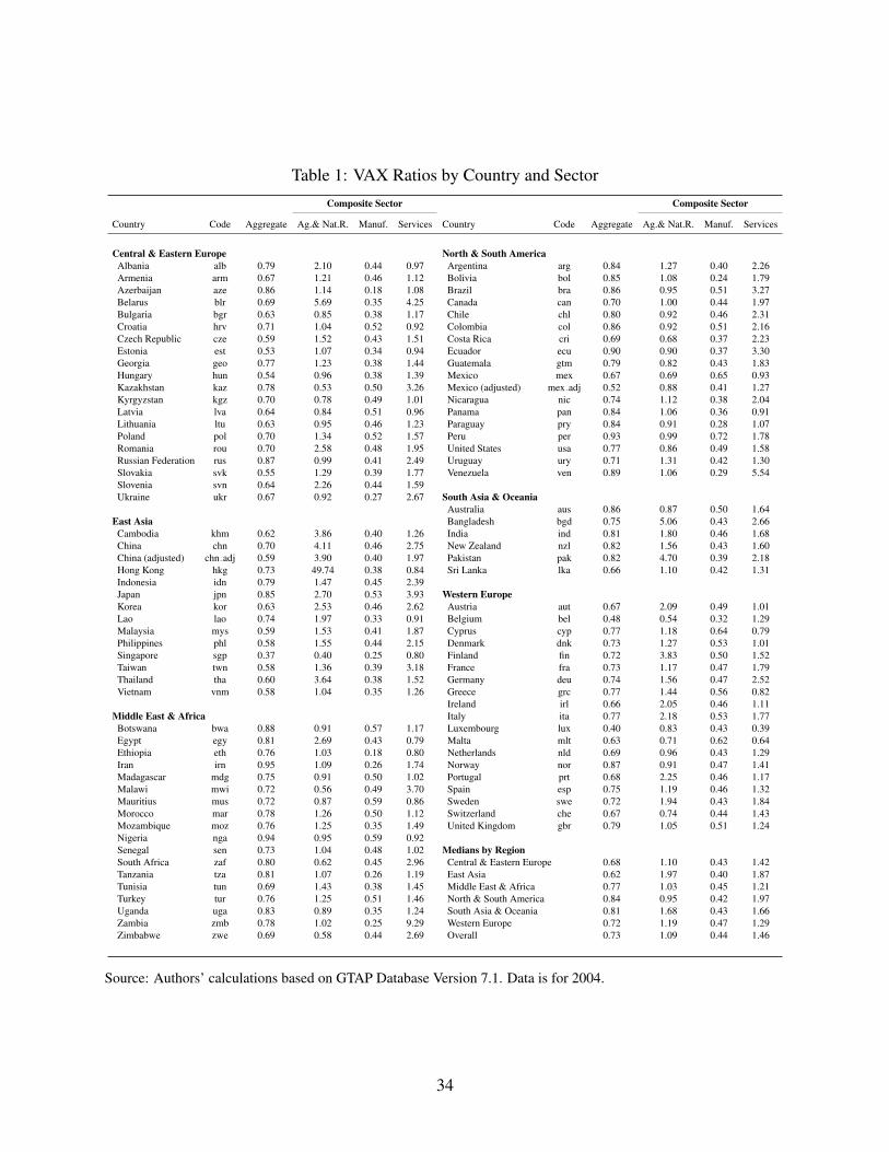
Table 1: VAX Ratios by Country and SectorComposite Sector Composite Sector

Country Code Aggregate Ag.& Nat.R. Manuf. Services Country Code Aggregate Ag.& Nat.R. Manuf. Services

Central & Eastern Europe North & South AmericaAlbania alb 0.79 2.10 0.44 0.97 Argentina arg 0.84 1.27 0.40 2.26Armenia arm 0.67 1.21 0.46 1.12 Bolivia bol 0.85 1.08 0.24 1.79Azerbaijan aze 0.86 1.14 0.18 1.08 Brazil bra 0.86 0.95 0.51 3.27Belarus blr 0.69 5.69 0.35 4.25 Canada can 0.70 1.00 0.44 1.97Bulgaria bgr 0.63 0.85 0.38 1.17 Chile chl 0.80 0.92 0.46 2.31Croatia hrv 0.71 1.04 0.52 0.92 Colombia col 0.86 0.92 0.51 2.16Czech Republic cze 0.59 1.52 0.43 1.51 Costa Rica cri 0.69 0.68 0.37 2.23Estonia est 0.53 1.07 0.34 0.94 Ecuador ecu 0.90 0.90 0.37 3.30Georgia geo 0.77 1.23 0.38 1.44 Guatemala gtm 0.79 0.82 0.43 1.83Hungary hun 0.54 0.96 0.38 1.39 Mexico mex 0.67 0.69 0.65 0.93Kazakhstan kaz 0.78 0.53 0.50 3.26 Mexico (adjusted) mex adj 0.52 0.88 0.41 1.27Kyrgyzstan kgz 0.70 0.78 0.49 1.01 Nicaragua nic 0.74 1.12 0.38 2.04Latvia lva 0.64 0.84 0.51 0.96 Panama pan 0.84 1.06 0.36 0.91Lithuania ltu 0.63 0.95 0.46 1.23 Paraguay pry 0.84 0.91 0.28 1.07Poland pol 0.70 1.34 0.52 1.57 Peru per 0.93 0.99 0.72 1.78Romania rou 0.70 2.58 0.48 1.95 United States usa 0.77 0.86 0.49 1.58Russian Federation rus 0.87 0.99 0.41 2.49 Uruguay ury 0.71 1.31 0.42 1.30Slovakia svk 0.55 1.29 0.39 1.77 Venezuela ven 0.89 1.06 0.29 5.54Slovenia svn 0.64 2.26 0.44 1.59Ukraine ukr 0.67 0.92 0.27 2.67 South Asia & Oceania

Australia aus 0.86 0.87 0.50 1.64East Asia Bangladesh bgd 0.75 5.06 0.43 2.66Cambodia khm 0.62 3.86 0.40 1.26 India ind 0.81 1.80 0.46 1.68China chn 0.70 4.11 0.46 2.75 New Zealand nzl 0.82 1.56 0.43 1.60China (adjusted) chn adj 0.59 3.90 0.40 1.97 Pakistan pak 0.82 4.70 0.39 2.18Hong Kong hkg 0.73 49.74 0.38 0.84 Sri Lanka lka 0.66 1.10 0.42 1.31Indonesia idn 0.79 1.47 0.45 2.39Japan jpn 0.85 2.70 0.53 3.93 Western EuropeKorea kor 0.63 2.53 0.46 2.62 Austria aut 0.67 2.09 0.49 1.01Lao lao 0.74 1.97 0.33 0.91 Belgium bel 0.48 0.54 0.32 1.29Malaysia mys 0.59 1.53 0.41 1.87 Cyprus cyp 0.77 1.18 0.64 0.79Philippines phl 0.58 1.55 0.44 2.15 Denmark dnk 0.73 1.27 0.53 1.01Singapore sgp 0.37 0.40 0.25 0.80 Finland fin 0.72 3.83 0.50 1.52Taiwan twn 0.58 1.36 0.39 3.18 France fra 0.73 1.17 0.47 1.79Thailand tha 0.60 3.64 0.38 1.52 Germany deu 0.74 1.56 0.47 2.52Vietnam vnm 0.58 1.04 0.35 1.26 Greece grc 0.77 1.44 0.56 0.82

Ireland irl 0.66 2.05 0.46 1.11Middle East & Africa Italy ita 0.77 2.18 0.53 1.77Botswana bwa 0.88 0.91 0.57 1.17 Luxembourg lux 0.40 0.83 0.43 0.39Egypt egy 0.81 2.69 0.43 0.79 Malta mlt 0.63 0.71 0.62 0.64Ethiopia eth 0.76 1.03 0.18 0.80 Netherlands nld 0.69 0.96 0.43 1.29Iran irn 0.95 1.09 0.26 1.74 Norway nor 0.87 0.91 0.47 1.41Madagascar mdg 0.75 0.91 0.50 1.02 Portugal prt 0.68 2.25 0.46 1.17Malawi mwi 0.72 0.56 0.49 3.70 Spain esp 0.75 1.19 0.46 1.32Mauritius mus 0.72 0.87 0.59 0.86 Sweden swe 0.72 1.94 0.43 1.84Morocco mar 0.78 1.26 0.50 1.12 Switzerland che 0.67 0.74 0.44 1.43Mozambique moz 0.76 1.25 0.35 1.49 United Kingdom gbr 0.79 1.05 0.51 1.24Nigeria nga 0.94 0.95 0.59 0.92Senegal sen 0.73 1.04 0.48 1.02 Medians by RegionSouth Africa zaf 0.80 0.62 0.45 2.96 Central & Eastern Europe 0.68 1.10 0.43 1.42Tanzania tza 0.81 1.07 0.26 1.19 East Asia 0.62 1.97 0.40 1.87Tunisia tun 0.69 1.43 0.38 1.45 Middle East & Africa 0.77 1.03 0.45 1.21Turkey tur 0.76 1.25 0.51 1.46 North & South America 0.84 0.95 0.42 1.97Uganda uga 0.83 0.89 0.35 1.24 South Asia & Oceania 0.81 1.68 0.43 1.66Zambia zmb 0.78 1.02 0.25 9.29 Western Europe 0.72 1.19 0.47 1.29Zimbabwe zwe 0.69 0.58 0.44 2.69 Overall 0.73 1.09 0.44 1.46

Source: Authors’ calculations based on GTAP Database Version 7.1. Data is for 2004.

34

Table 2: Aggregate and Manufacturing VAX Decompositions

Panel A: Aggregate VAX DecompositionV AXi − V AX Within Term Between Term

Log Income Per Capita -0.008 0.028** -0.036***(0.005) (0.011) (0.013)

R2 0.02 0.07 0.08N 90 90 90

Panel B: Manufacturing VAX DecompositionV AXi − V AX Within Term Between Term

Log Income Per Capita 0.018*** -0.007 0.025***(0.006) (0.009) (0.008)

R2 0.11 0.01 0.12N 89 89 89

Robust standard errors are in parentheses. Significance levels: * p < .1 , ** p < .05, ***p < .01. Constants included in all regressions. Income per capita equals exporter value addedper capita, where value added is calculated using our data and population is from the GTAP7.1 database. Belgium, Luxembourg, and Singapore excluded in Panel A and Botswana, HongKong, Paraguay, and Peru excluded in Panel B as outliers.

Table 3: Bilateral VAX Ratio: Bilateral HIY vs. Production Sharing Adjustment

Variance Decomposition

Exporter BHIY Term PSA Term

U.S. 5% 95%Germany 5% 95%Japan 1% 99%China 9% 91%

Argentina 1% 99%France 8% 92%Hungary 5% 95%India 7% 93%Portugal 9% 91%

Median Country 3% 97%

See the text for details regarding the decomposition.The Median Country is the median statistic for all 93countries in the data.

35

Table 4: Decomposing Trade: Absorption, Reflection, and Redirection

Japan exports to: U.S. exports to:China U.S. Mexico Canada

China 64.5% U.S. 92.7% Mexico 72.3% Canada 68.9%U.S. 11.1% Canada 1.4% U.S. 22.1% U.S. 24.1%Japan 4.3% Mexico 0.7% Canada 0.9% U.K. 0.7%Germany 2.5% Japan 0.6% Germany 0.4% Japan 0.7%

Germany exports to: Korea exports to:France Czech Rep. China Japan

France 74.8% Czech Republic 57.7% China 61.3% Japan 83.1%Germany 3.6% Germany 11.7% U.S. 12.1% U.S. 4.7%U.K. 2.8% U.K. 3.0% Japan 4.7% China 2.3%U.S. 2.6% U.S. 2.6% Germany 2.7% Germany 1.0%

See the text for details regarding the decomposition. The entries in the table describe the approximate shareof bilateral exports to each destination that are ultimately consumed in that destination. Shares do not sum toone because we include only the top four destinations for each bilateral pair. Data is for 2004.

0.2

.4.6

.81

Sh

are

bel can chn deu fra gbr ita jpn kor usa

Manufactures

0.2

.4.6

.81

Sh

are

bel can chn deu fra gbr ita jpn kor usa

Services

Export Share Value Added Export Share

Figure 1: Composite Sector Shares of Gross Exports and Value Added Exports, by Country (2004)

36

Figure 2: Between-Within Decomposition of Aggregate VAX Ratios, by Country (2004)

0.2

.4.6

.81

1.2

1.4

Ra

tio o

f Va

lue

Ad

de

d to

Gro

ss

Tra

de

mex_adj sgp mys irl can mex bel chn_adj twn kor chn bra deu gbr fra jpn ita aus esp rus

United States Bilateral Trade

0.2

.4.6

.81

1.2

1.4

Ra

tio o

f Va

lue

Ad

de

d to

Gro

ss

Tra

de

bel hun cze che aut irl chn_adj pol nld swe fra chn esp ita gbr rus usa can jpn aus

Germany Bilateral Trade

Exports Imports

Figure 3: Value Added to Gross Trade Ratios for the United States and Germany, by Partner (2004)

37

-13

0-1

20

-11

0-1

00

-90

-80

-70

-60

-50

-40

-30

-20

-10

01

0

US

D B

illi

on

s

chn jpn can deu mys ita twn gbr mex kor irl bra rus fra bel esp sgp aus

Trade Deficit

Value Added Deficit

Adjusted Value Added Deficit

Figure 4: Bilateral Trade and Value Added Balances for the United States, by Partner (2004)

38

Appendix A

The basic idea behind the adjustment for processing trade is to split the aggregate economy into

separate processing and non-processing units, each with its own input-output structure. Both sec-

tors use domestic and imported intermediates, but they differ in terms of intermediate input inten-

sity and the source (domestic versus imported) of intermediates. Further, all output in the export

processing sector is exported.

From the input-output data, we observe the domestic intermediate use matrix mii and import

use matrix asmIi for the economy as a whole. From trade data, we observe total exports originating

from and imported intermediates used by the processing sector, denoted xPi and mPIi respectively.

Output in the non-processing sector, denoted yNi , is calculated by subtracting xPi from total out-

put in the input-output accounts. We seek separate intermediate use matrices for the two sectors

{mNii ,m

Pii ,m

NIi,m

PIi} and value added by sector {vaNi , vaPi } that satisfy:

mii = mNii +mP

ii (A1)

mIi = mNii +mP

Ii (A2)

yNi = vaNi + ι[mNii +mN

Ii

](A3)

xPi = vaPi + ι[mPii +mP

Ii

](A4)

mPIi = mP

Iiι′, (A5)

where ι is a conformable row vector of ones and ι′ is its transpose.50

If there are N sectors, then there are 4(N×N)+2N unknowns and only 2(N×N)+3N con-

straints so we cannot solve directly for the unknown coefficients. We therefore follow Koopman,

Wang, and Wei (2008) and use a constrained minimization routine to impute the unknown coef-

ficients, where the objective function minimizes squared deviations between imputed values and

target values. Target values are set by splitting intermediate use and value added across processing

50These constraints differ from those used by Koopman, Wang, and Wei (2008) in that we use the domestic andimport intermediate use matrices separately, whereas they pool this information into a single overall use matrix.

39

and non-processing sectors according to their shares in total output.

With the resulting split tables, we use bilateral trade data as in the main text to construct bi-

lateral sourcing matrices and the global input-output table.51 In performing the calculation, we

use processing trade shares from Koopman, Wang, and Wei (2008) for China. For Mexico, we

obtain trade data for the maquiladora sector from the Bank of Mexico.52 Due to concerns about the

quality of disaggregate data and the accuracy of the imputation procedure for individual sectors,

we aggregate the data to 3 composite sectors prior to imputing coefficients. Because bilateral value

added trade results are essentially identical in the main data when computed with 57 sectors or 3

composite sectors, we believe aggregation does not result in diminished accuracy.

51In the resulting system, China and Mexico effectively have 2N sectors, where each of the N sectors is separatedinto processing and non-processing sub-sectors.

52Data is availabe at: http://www.banxico.org.mx/polmoneinflacion/estadisticas/balanzaPagos/balanzaPagos.html.

40