accounting for forecast uncertainty in policy making
TRANSCRIPT
CE295 – Energy Systems and Control Professor Scott Moura
1
Accounting For Forecast Uncertainty In Policy Making: China's
Electricity Pathways By 2050
Anne-Perrine Avrin
University of California, Berkeley
Spring 2015
“There are risks and costs to action, but they are far less than the long range risks of comfortable inaction.” John F. Kennedy
Abstract
While the tremendous number of alternate scenarios for the future global energy mix is overwhelming,
tools are critically needed to dynamically evaluate the energy, carbon, costs, and risks associated with each
option. The various ‘optimal’ pathways identified by existing cost-minimizing energy planning tools
demonstrate amplitudes in nature and cost difference that almost span the entire range of options initially
faced by governments while, too often, forecast uncertainty is overlooked. The slow transition of the
world’s energy generation is due in part to our inability to weigh, trust and choose among least-cost
scenarios. We develop a versatile two-step methodology to help policy makers adjust for risks on costs their
findings from cost-minimization modeling tools, while sparing them the hurdles of adopting a new model.
We formulate a quadratic programming add-on with MATLAB to minimize risks of the Chinese least-cost
electricity pathway over the 2050 horizon identified by the cost-minimizing tool SWITCH. We find that,
in 2030, it is possible to decrease the least-cost portfolio’s annual risks on costs by 2.3% - $5 billion - while
increasing total electricity costs by less than half - $2 billion. Between 2045 and 2054, we study the
development of a new technology: the fast neutron nuclear reactor, and recognize that, despite its high
uncertainty on overnight cost projections, its integration yields a reduction in risks on the total electricity
costs of 38%. We observe that the uncertainty of future pollution regulation, or ‘fear of regulation’, can reduce carbon emissions by at least 10% in 2050.
I. INTRODUCTION
In 2012, global electricity consumption was 19,500 TWh [1] and CO2 emissions from the power sector
accounted for 13 Gt [2], or 42% of the total carbon emissions in that year. The global electricity demand is
projected to reach 35,000 TWh by 2040. The ability of the world to meet its growing electricity demand
while reducing the carbon intensity of its energy production, in order to spare the climate and the
environment, will depend on what actions countries take now and in the next decades.
The foundation of this study is based on the recognition that, for policy makers, optimizing an electricity
portfolio is a trade-off between the minimization of cost – or “affordability” – and the minimization of uncertainty on costs – or “risk”.
Given the large amount of parameters that needs to be considered in order to optimize investment in a
country’s future energy mix, modeling tools have been developed to help governments and stakeholders
plan long-term expansion of the power sector. The most common methodology for optimization and
modeling of energy systems is mathematical programming (MP) [3]. Traditional energy planning tools have
a cost-minimization objective [4], usually based on linear programming (LP), subject to constraints such as
projected demand, cap on carbon emissions or other types of pollutants, or carbon tax.
CE295 – Energy Systems and Control Professor Scott Moura
2
A continuous challenge that arises when researchers employ projection on future costs, embedding
uncertainty, to design scenarios for the energy mix is: to what extent the information given by the least-cost
pathway(s) for policy-making purposes is impacted by the uncertainty on cost projections? Unlike
modelers, policy makers use energy-planning tools to evaluate the consequences of developments and
policy choices before their application [5]. The objective of modelers depends on the structure of the
modeling tool, and minimizing cost can be as sensible as minimizing risk or any other variable. On the
other hand, the main objective of policy makers is to maximize the expected utility, which is impacted by
both costs and risks, and modeling tools must be as comprehensive as possible to constitute a valuable mean
to identify the best pathway to reach this goal. While the success of modelers can be evaluated through the
sophistication of the model, a successful model for policy makers can be summarized by this sentence “One
strategy to stay clear of the pitfalls of modeling would be to attempt to learn from a model in a way that the lessons learned would be explainable without explaining the model.” [6]
Over the last decades, significant progress has been made on the capacity and size of data set that can be
handled by modeling tools, improving their temporal and spatial resolution. While the scientific value of
this progress cannot be denied, it does not necessarily lead to tools that better suit policy makers’ needs. In
fact, dealing with uncertainty on projections requires additional data than those currently used by LP
models, different in nature but not necessarily in size. Many linear programs aiming at minimizing costs do
not optimize over risks on costs, leading to another kind of risk: a “Garbage In, Garbage Out”, or GIGO,
situation. Yet, ensuring that the future cost of electricity will fall into a reasonable tolerance interval around
the forecasted cost might be as much valued by governments as minimizing of the most-likely electricity
cost itself in the search for the optimal energy mix.
The common way to address uncertainty in energy planning modeling tools is the use of scenarios [6] or
sensitivity analysis, such as in the HOMER model [7]. The amplitude of these approaches is limited as
variability of costs is expressed in the outputs rather than in the inputs, and is qualitative rather than quantitative.
Yet, some modeling tools are designed to minimize uncertainty on projections through stochastic methods
such as Monte Carlo simulations, or through mean-variance analyses. The main differences between these
two approaches lies in the fact that the former is based on simulations while the latter is based on
optimization. Stochastic methods might seem to be the most straightforward approach as they complement
the cost-minimization approach by simulating a range of possible costs for a given scenario. If the number
of runs is high enough, trends can be identified and the error margin can be significantly decreased.
However, the main caveat arising when dealing with Monte Carlo is the impossibility to ensure that cliff
edge effects have been identified, as the range of outcomes resulting from the simulations is discrete rather
than continuous.
Mean-variance optimization poses some reliability challenges too, as it often assumes no uncertainty on the
uncertainty: the standard deviation is supposed to be known with precision. While this can be problematic
in some branches of finance subject to a selection bias, for example for private capital returns when firms
that go out of business no longer report to them [8], the centralized long-term expansion planning of a
national or international energy mix is usually not subject to this bias. Past data that energy planners rely
on to create cost projections is comprehensive. It is based on publicly available, or at least government-
own, data such as historical market prices of fuel and past construction and operation costs of energy
systems. While the average values of this past data cannot, by any mean, be considered as an accurate
prediction of future costs, the typical scope embraced is old and large enough to represent an accurate
landscape of the range of possibilities of future costs. For these reasons, we choose mean-variance optimization over Monte Carlo simulation for the current study.
CE295 – Energy Systems and Control Professor Scott Moura
3
China’s energy system is an ideal laboratory to study this evolution because the country presents a
centralized power sector facilitating the optimization of the mix at the national scale, and because the extent
of its future demand is such that electricity supply will require the development of novel, unconventional
technologies, for which taking risk on generation cost into account is crucial.
The first section of this paper presents the methodology developed and the description of the quadratic
program formulated for performing the mean-variance portfolio analysis. The second section deals with the
characterization of risks on levelized cost of electricity projections (LCOE); calculations are illustrated by
the example of China’s energy mix costs projections. The third section is a case study of the two-step
optimization process applied to the Chinese power sector with the use of the SWITCH-China modeling tool.
II. RELEVANT LITERATURE
The literature on multi-objective optimization in the fields of economics and finance has developed since
the 1950’s [9] and is now extensive [10] [11]. From their original purpose, modern portfolio theory (MPT)
and two-moment decision modeling have been extended to other contexts, different in goals but presenting
a similar structure. The application of MTP to energy portfolio management is a relatively new field that
has significantly expanded these last years [12] [13] [14] [15], together because of increasing awareness of
potential environmental impacts of energy production systems and subsequent limiting regulations, novel
electricity generation technologies resulting in more uncertain investment risk and return, and deregulation
of electricity markets. Such studies dealing with the power sector tend to favor the development of
renewable energies in conventional, often fossil fuel-based, energy systems because of fuel price volatility
[16] and because of the positive impact of diversification on risk reduction. On the contrary, the variability
in costs of renewables is often underestimated by the use of average capacity factor over time and space.
These loose assumptions lead to important discrepancies between Pareto optima modeled with different
beliefs, as shown by these two analyses performed on the Chinese power sector [17] [18]. The novelty of
the current study lies in several areas. First, we propose a high-fidelity method as we constrain the risk-
minimization analysis in order to preserve the grid reliability ensured by the high-resolution linear program
SWITCH. Second, we use several hundred thousand historical hourly capacity factors for central PV and
wind turbines in China in order to accurately design the magnitude of the uncertainty resulting from
renewable energy intermittency. Third, as the focus of our study is to improve the quality of long-term
planning for the energy mix from a policy making perspective, we create an original two-step process to ensure an easy adoption of the tool by policy makers.
III. METHODOLOGY
Cost-minimization tools, often based on LP, bring valuable insight into the type, or ‘nature’, of the optimal
pathway for planning expansion of the power sector while ensuring that costs remain reasonable. However,
because of uncertainty on cost projections, the economic stability of the ‘reasonable costs’ cannot be
ensured. Among a set of expansion trajectories for the future energy mix, whose costs of electricity are
similar yet not identical, LP modeling tools invariably choose the cheapest scenario. In reality, policy
makers seek to include in their decision-making the likelihood that the real cost would remain close to the
projected cost if the considered scenario were implemented. As detailed in the previous section, most long-
term modeling tools used by policy makers today focus on a minimization of costs subject to constraints such as growing demand, cap on some energy sources, and carbon cap or tax.
CE295 – Energy Systems and Control Professor Scott Moura
4
Creating a dual tool simultaneously minimizing costs and risk on costs would surely prove to be a very
valuable asset for long-term planning of the energy mix. However, given the myriad of existing models
presenting various – sometimes very similar – approaches for the energy mix, and the adaptation time that
would be required to transition the new modeling tool from a research-based usage to a policy-making usage, a new approach must be developed.
The complex, high-resolution, LP tools currently used by policy makers to identify least-cost generation
expansion pathways constitute valuable assets as they usually both define the ’nature’ of the future energy
mix and perform a comprehensive analysis to ensure the reliability of the grid at different time scales. By
setting a sufficiently narrow range of allowed deviations around the generation levels from each energy
source of the least-cost portfolios, defining a ‘safety net’, it is possible to minimize risks while not impacting
the ‘nature’, therefore the reliance, of the energy production and supply mix ensured by the LP tools.
Our hypothesis is that policy makers could comprehensively plan expansion of the energy mix through two
successive steps. The first step, which is generally performed by most energy planners, involves the
identification of optimal electricity generation levels form each considered energy source or technology,
via a thorough linear cost optimization with an existing modeling tool. The second step would consist in
allowing slight deviations around the least-cost energy pathways in order to optimize the risks on costs of
the future energy mix. The final objective is to develop a new approach to refine results of optimal
generation levels obtained from complex cost-minimizing modeling tools by confronting them against a
simpler risk-minimization model, while restricting deviation from the least-cost pathway findings in order to ensure that the designed grid remains reliable.
A. Quadratic-programming model description Mean-variance portfolio analysis (MVPA) uses variance on costs as the metrics to evaluate risks. For this
study, we define the expected generation cost of an energy system technology as the mean of the cost
projection distribution. The expected electricity cost of an energy portfolio is the weighted average of the
individual expected cost of each energy technology. Similarly, the expected risk on generation cost of a
technology is characterized by the variance - or its square root, the standard deviation - of the projected
cost. The expected overall risk on cost of an energy portfolio is the weighted average of the individual risks,
characterized for each technology by the square value of the standard deviation of cost multiplied by the
generation share of the technology. The program formulated in this study is, by definition, a quadratic
program. Since it constitutes a module to be used as second step after a thorough cost-minimization
optimization, it must be as simple as possible and not redundant with the first step. The LP involved in the
first step is assumed to optimize transmission lines, storage capacity, and hourly dispatch of the electricity
grid, in order to ensure the reliability of the grid, therefore these components are not taken into account in
the QP. The ‘safety net’ within which the QP can act in order to minimize risk without jeopardizing the
grid reliability is outlined by boundaries of plus and minus 10% around the generation levels of each energy
technology in the least-cost portfolio calculated by the LP. We choose 10% because it is low enough that,
for any energy system technology, the additional capacity potentially calculated by the QP compared to the
least-cost portfolio can be installed on existing sites – or new sites already modeled by the LP – eliminating
the need to take into account additional infrastructure costs not considered in the QP. Therefore, we assume
in this study that no additional transmission lines are needed if the capacity of an electricity production site is increased by up to 10%.
The mathematical definition of the problem and notation are presented below.
The objective function is:
CE295 – Energy Systems and Control Professor Scott Moura
5
𝑚𝑖𝑛∑𝑥𝑖𝑇 × 𝜎𝑖
2 × 𝑥𝑖
9
𝑖=1
Subject to the constraints:
Electricity produced from each technology cannot be negative: ∀𝑖,𝑥𝑖 ≥ 0
Generation share of each technology must be within +/- 10% of the least-cost portfolio values:
∀𝑖, 0.9𝑥𝑆 ≤ 𝑥𝑖 ≤ 1.1𝑥𝑆
The electricity mix is subject to a carbon cap: ∑ 𝑒𝑖 ×𝑥𝑖 ≤ 𝐸𝑛𝑖=1
Total cost must equal a certain value: ∑ 𝑐𝑖 × 𝑥𝑖 = 𝑇𝐶𝑛𝑖=1
Wind and solar standard intermittency deviation must be backed up by peaker plants: 𝜎𝑤𝑖𝑛𝑑 ×
𝑥𝑤𝑖𝑛𝑑 + 𝜎𝑠𝑜𝑙𝑎𝑟 ×𝑥𝑠𝑜𝑙𝑎𝑟 − 𝑥𝑔𝑎𝑠 ≤ 0
Electricity generated from hydro pumped, hydro non-pumped and nuclear is capped at the
SWITCH generation level (for availability reasons for hydro, and logistics reasons regarding
construction of nuclear power plants): ∀𝑖 ∈ [5;7], 𝑥𝑖 ≤ 𝑥𝑆
Annual demand must be met: ∑ 𝑥𝑖 = 𝐷𝑛𝑖=1
Which translates into the quadratic program:
min1
2𝑥𝑇𝑄𝑥+ 𝑅𝑇𝑥
𝑠. 𝑡. 𝐴𝑥 ≤ 𝑏 𝑎𝑛𝑑 𝐴𝑒𝑞𝑥 = 𝑏𝑒𝑞
Table 1 Notation used to formulate the quadratic problem
xi Share of electricity produced from technology i (MWh)
x Vector of shares of electricity generation levels [nx1] xS Vector of shares of electricity generation levels in the least-cost
portfolio [nx1]
Ci Generation cost of technology i ($/MWh) TC Total cost of production of the portfolio ($)
Q Covariance matrix [nxn] R Linear portion of the cost function [9x1] (null here)
A Inequality constraint matrix (right-hand side) [mx9] b Inequality constraint matrix (left-hand side) [mx1]
Aeq Equality constraint matrix (right-hand side) [lx9] Beq Equality constraint matrix (left-hand side) [lx1]
ei Rate of CO2 emissions from technology i (tCO2/MWh) E Annual carbon cap (tCO2)
D Annual electricity demand
IV. CHARACTERIZATION OF THE RISK: DATA AND
STANDARD DEVIATION OF COSTS.
The cost projections implemented in this project come from data used in the cost-minimizing SWITCH-
China modeling tool. The characteristics of the mixed integer linear program SWITCH are described in
CE295 – Energy Systems and Control Professor Scott Moura
6
details in the Case study section of this study. SWITCH inputs consist in average projected values of
different cost components such as overnight costs, variable and fixed operation and maintenance costs
including projections on fuel prices, and a discount rate of 8%. In the rest of this study, calculations will be
illustrated with the case of the Chinese power sector, with a simplified electricity mix including nine
technologies: coal steam turbine, gas combustion turbine, wind turbine, solar central PV, combined cycle gas turbine, generation II/III nuclear reactor and, from 2045 on, generation IV fast neutron nuclear reactors.
A. Levelized Cost of Electricity The cost projections used in SWITCH-China have been obtained from various sources such as international
institutions, governmental entities, universities, and private companies. For each cost component, the data source is given in [19].
In order to simplify the QP, for the reasons presented above, a unique cost figure is needed per technology
per year. The LCOE is a convenient metrics, representing the average cost of producing electricity from a
specific generation technology over its financial lifetime. The calculation of the LCOE per technology per
year is calculated for all the technologies considered in this study, based on the EIA method [20] and the SWITCH-China inputs. The formula to calculate LCOE is:
𝐿𝐶𝑂𝐸 =
∑𝐼𝑡 + 𝑀𝑡 + 𝐹𝑡
(1 + 𝑟)𝑡𝑛𝑡=1
∑𝐸𝑡
(1 + 𝑟)𝑡𝑛𝑡=1
Where:
It is the investment expenditure in year t,
Mt is O&M expenditure in year t,
Ft is fuel expenditure in year t,
Et is electricity generation in year t,
r is the discount rate,
n is the lifetime of the system.
The average values of overnight costs, operation and maintenance costs, and fuel prices of conventional
generation plants such as gas combustion turbines, coal steam turbines and Generation II and III nuclear
reactors are assumed to remain stable over the next decades, resulting in a flat LCOE curve for these
technologies. The cost of technologies whose large-scale development is more recent, such as wind
turbines, central PV and, from 2030 on, fast neutron reactors, is assumed to decrease according to a learning curve of 0.5% on average for wind and solar technologies, and 1.6% for generation IV nuclear power.
B. Quantification of the risk on LCOE The quantification of risks is performed through two consecutive steps: identification of standard deviations
on various cost components (in %) for each technology, and the translation of these standard deviations
into a unique standard deviation of LCOE expressed in $/MWh.
The following factors of uncertainty are taken into account:
Uncertainty on overnight costs (σovernight),
Uncertainty on fuel cost resulting from fuel price volatility (σfuel),
Uncertainty on fixed operation and maintenance costs, including potential future safety regulations
for nuclear power (σO&M),
CE295 – Energy Systems and Control Professor Scott Moura
7
Uncertainty on renewable output resulting from intermittency of wind and solar (σintermittent),
Uncertainty on future regulations on CO2 emissions and other pollutants.
Cost components for each technology are assumed to be independent [21]. Correlations between risks are set to zero in this study.
The main drivers of risks in China for gas combustion turbines and, to a lesser extent, for coal steam
turbines, are future fuel price volatility and future regulation on CO2 emissions. For wind turbines and solar
PV, risks mainly result from intermittency. Risks on generation costs from nuclear power are driven by
uncertain overnight costs and potential future safety regulation. The fuel efficiency of fast neutron reactors
is, on average, 60 times higher than the fuel efficiency of Generation III nuclear reactors. We assume that
risk on nuclear fuel cost results from uncertain future uranium prices only. As a consequence, standard
deviation of FNR fuel is 60 times lower than for conventional nuclear power. Hydro pumped and non-
pumped generators present very low risks compared to the other technologies. Several studies provide
values for standard deviations on various cost components of generation technologies [4] [12] [15] [17] [18] [21] [22] [23] for different countries. These values are updated and adapted to the case of China.
While the risk on costs resulting from intermittency of variable renewable energies have not, to the best of
our knowledge, be taken into account in published articles on MVPA for the energy mix, here we present a methodology to calculate the standard deviations resulting from the variability renewable energies.
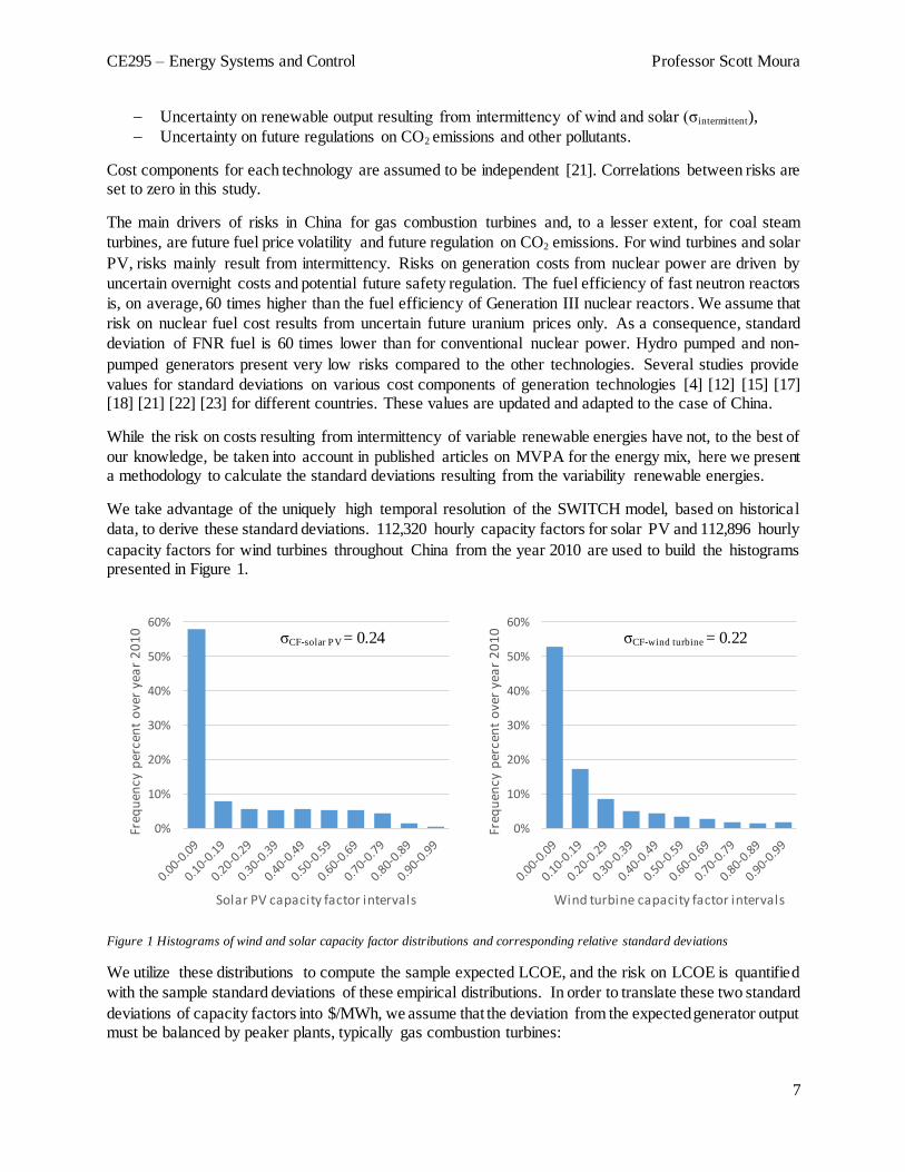
We take advantage of the uniquely high temporal resolution of the SWITCH model, based on historical
data, to derive these standard deviations. 112,320 hourly capacity factors for solar PV and 112,896 hourly
capacity factors for wind turbines throughout China from the year 2010 are used to build the histograms presented in Figure 1.
We utilize these distributions to compute the sample expected LCOE, and the risk on LCOE is quantified
with the sample standard deviations of these empirical distributions. In order to translate these two standard
deviations of capacity factors into $/MWh, we assume that the deviation from the expected generator output must be balanced by peaker plants, typically gas combustion turbines:
0%
10%
20%
30%
40%
50%
60%
Freq
uen
cy p
erce
nt
ove
r ye
ar
20
10
Wind turbine capacity factor intervals
0%
10%
20%
30%
40%
50%
60%
Freq
uen
cy p
erce
nt
ove
r ye
ar
20
10
Solar PV capacity factor intervals
σCF-solar PV = 0.24 σCF-wind turbine = 0.22
Figure 1 Histograms of wind and solar capacity factor distributions and corresponding relative standard deviations
CE295 – Energy Systems and Control Professor Scott Moura
8
𝜎𝑖𝑛𝑡𝑒𝑟𝑚𝑖𝑡𝑡𝑒𝑛𝑐𝑦 𝑐𝑜𝑠𝑡−𝑡𝑒𝑐ℎ𝑛𝑜𝑙𝑜𝑔𝑦 𝑖−𝑦𝑒𝑎𝑟 𝑦 ($ 𝑀𝑊ℎ⁄ )
= 𝜎𝐶𝐹−𝑡𝑒𝑐ℎ𝑛𝑜𝑙𝑜𝑔𝑦 𝑖 (𝑛𝑜 𝑢𝑛𝑖𝑡) × 𝐿𝐶𝑂𝐸𝑔𝑎𝑠−𝑦𝑒𝑎𝑟 𝑦 ($ 𝑀𝑊ℎ⁄ )
The uncertainty on the other cost components are translated from % to $/MWh by multiplying the standard
deviations with the corresponding future expected value of the cost component projected in the same unit.
The standard deviations are then aggregated to create a unique standard deviation representing the risk on LCOE per technology per year, expressed in $/MWh.
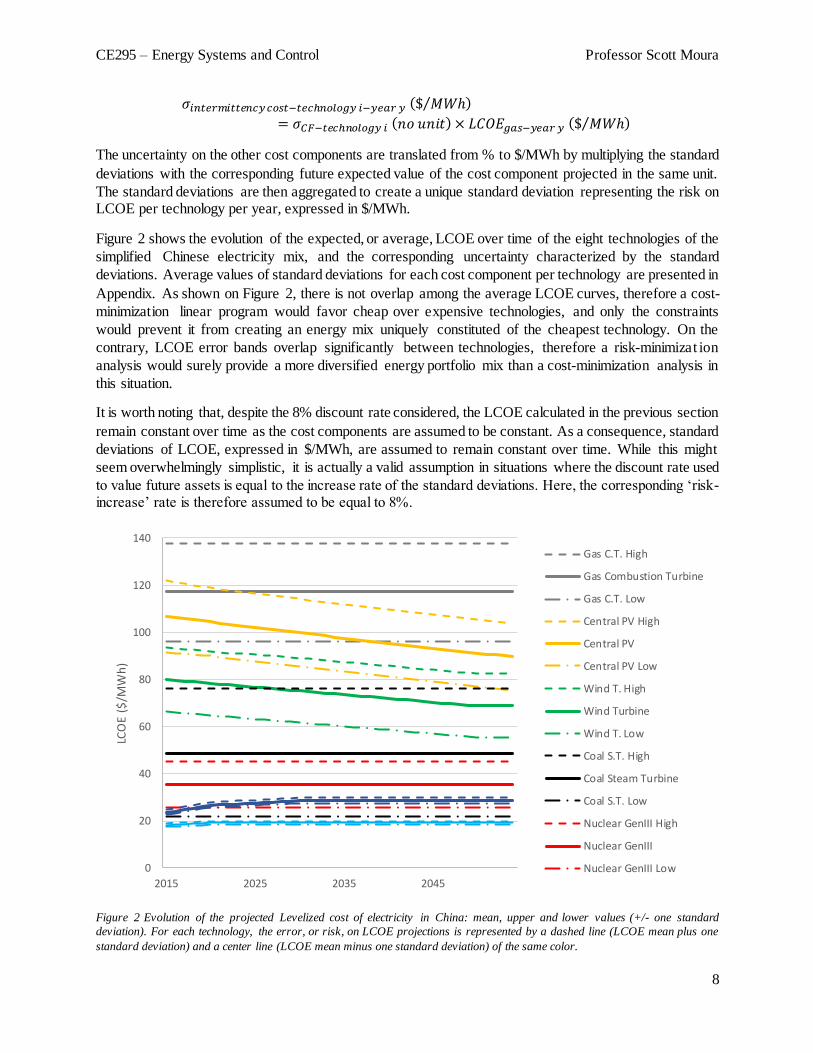
Figure 2 shows the evolution of the expected, or average, LCOE over time of the eight technologies of the
simplified Chinese electricity mix, and the corresponding uncertainty characterized by the standard
deviations. Average values of standard deviations for each cost component per technology are presented in
Appendix. As shown on Figure 2, there is not overlap among the average LCOE curves, therefore a cost-
minimization linear program would favor cheap over expensive technologies, and only the constraints
would prevent it from creating an energy mix uniquely constituted of the cheapest technology. On the
contrary, LCOE error bands overlap significantly between technologies, therefore a risk-minimizat ion
analysis would surely provide a more diversified energy portfolio mix than a cost-minimization analysis in
this situation.
It is worth noting that, despite the 8% discount rate considered, the LCOE calculated in the previous section
remain constant over time as the cost components are assumed to be constant. As a consequence, standard
deviations of LCOE, expressed in $/MWh, are assumed to remain constant over time. While this might
seem overwhelmingly simplistic, it is actually a valid assumption in situations where the discount rate used
to value future assets is equal to the increase rate of the standard deviations. Here, the corresponding ‘risk-increase’ rate is therefore assumed to be equal to 8%.
Figure 2 Evolution of the projected Levelized cost of electricity in China: mean, upper and lower values (+/- one standard
deviation). For each technology, the error, or risk, on LCOE projections is represented by a dashed line (LCOE mean plus one
standard deviation) and a center line (LCOE mean minus one standard deviation) of the same color.
0
20
40
60
80
100
120
140
2015 2025 2035 2045
LCO
E ($
/MW
h)
Gas C.T. High
Gas Combustion Turbine
Gas C.T. Low
Central PV High
Central PV
Central PV Low
Wind T. High
Wind Turbine
Wind T. Low
Coal S.T. High
Coal Steam Turbine
Coal S.T. Low
Nuclear GenIII High
Nuclear GenIII
Nuclear GenIII Low
CE295 – Energy Systems and Control Professor Scott Moura
9
V. CASE-STUDY: OPTIMAL EVOLUTION OF THE CHINESE
ELECTRICITY MIX OVER THE 2050 HORIZON
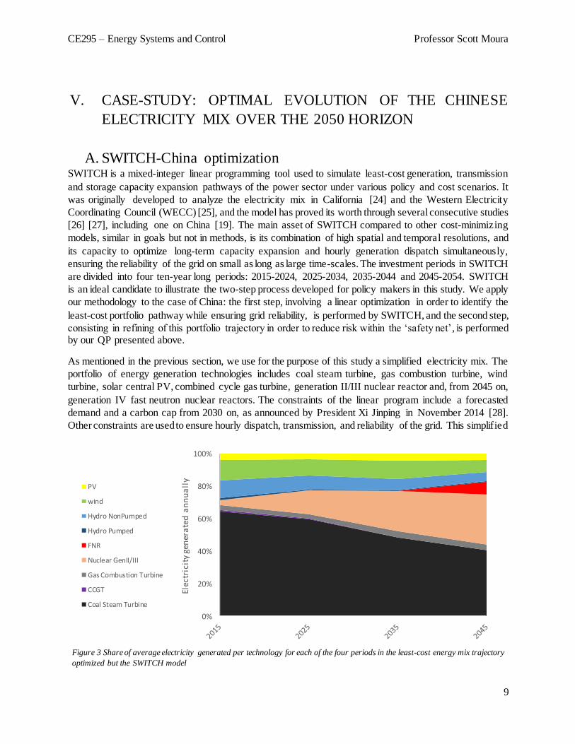
A. SWITCH-China optimization SWITCH is a mixed-integer linear programming tool used to simulate least-cost generation, transmission
and storage capacity expansion pathways of the power sector under various policy and cost scenarios. It
was originally developed to analyze the electricity mix in California [24] and the Western Electricity
Coordinating Council (WECC) [25], and the model has proved its worth through several consecutive studies
[26] [27], including one on China [19]. The main asset of SWITCH compared to other cost-minimizing
models, similar in goals but not in methods, is its combination of high spatial and temporal resolutions, and
its capacity to optimize long-term capacity expansion and hourly generation dispatch simultaneously,
ensuring the reliability of the grid on small as long as large time-scales. The investment periods in SWITCH
are divided into four ten-year long periods: 2015-2024, 2025-2034, 2035-2044 and 2045-2054. SWITCH
is an ideal candidate to illustrate the two-step process developed for policy makers in this study. We apply
our methodology to the case of China: the first step, involving a linear optimization in order to identify the
least-cost portfolio pathway while ensuring grid reliability, is performed by SWITCH, and the second step,
consisting in refining of this portfolio trajectory in order to reduce risk within the ‘safety net’, is performed by our QP presented above.
As mentioned in the previous section, we use for the purpose of this study a simplified electricity mix. The
portfolio of energy generation technologies includes coal steam turbine, gas combustion turbine, wind
turbine, solar central PV, combined cycle gas turbine, generation II/III nuclear reactor and, from 2045 on,
generation IV fast neutron nuclear reactors. The constraints of the linear program include a forecasted
demand and a carbon cap from 2030 on, as announced by President Xi Jinping in November 2014 [28].
Other constraints are used to ensure hourly dispatch, transmission, and reliability of the grid. This simplified
0%
20%
40%
60%
80%
100%
Elec
tric
ity
gen
era
ted
an
nu
all
y
PV
wind
Hydro NonPumped
Hydro Pumped
FNR
Nuclear GenII/III
Gas Combustion Turbine
CCGT
Coal Steam Turbine
Figure 3 Share of average electricity generated per technology for each of the four periods in the least-cost energy mix trajectory
optimized but the SWITCH model
CE295 – Energy Systems and Control Professor Scott Moura
10
energy mix is simulated with SWITCH for the purpose of this study in order to obtain the least-cost expansion trajectory for the power sector. The share of generation per technology is presented in Figure 3.
Early retirement of operating plants is not considered in this study. Therefore, the risk minimization analysis
is performed over electricity generation from new plants only. By ‘new plants’, we mean all electricity
generation systems built in the SWITCH model as a result of the optimization problem only, that is, plants
that were not already built and operating before 2015. The only exception is hydro generators, whose
generation levels can be adjusted through the risk analysis, as in China they are more constrained by the
fuel availability than by the construction and operation challenges of the systems. The quantity of electricity
generated from hydro (Hydro pumped, Hydro non pumped) and new plants (Coal steam turbine, Gas
combustion turbine, Wind turbine, Solar PV, GenII/III LWR nuclear reactor and Fast Neutron Reactors) is
given for the four periods in the column matrices below. Fast neutron reactors can only be built in the fourth
period. Following this optimization, the resulting annual electricity generation per technology in the least-
cost pathway, averaged over each period, is used as input in the QP. Each of the four vectors presented
below corresponds to a specific ten-year long period, and the rows represent the annual electricity
generation from Coal steam turbine, Gas combustion turbine, Hydro pumped, Hydro non pumped, Wind
turbine, Solar PV and GenII/III nuclear reactor, respectively, averaged over the entire period. The last row of the last vector (2045-2054 period) corresponds to Fast Neutron Reactors.
𝑥2015−2024 = 106
[ 2373262935319829150 ]
; 𝑥2025−2034 = 106
[ 42312801005365638921284]
; 𝑥2035−2044 = 106
[ 47434781466521588942902]
; 𝑥2045−2054 = 106
[ 535853511125854888744821183]
For each period, the corresponding annual electricity demand that new plants must meet is 4887 TWh, 8121
TWh, 1106 TWh, 1419 TWh, and the carbon cap 2.42x10⁹ tCO2, 4.02x10⁹ tCO2, 4.66x10⁹ tCO2, 5.01x10⁹ tCO2, respectively.
B. Risk minimization
‘Static’ optimization: minimizing the risk of China’s energy portfolio in
2030 A static version of the quadratic program is first formulated with MATLAB, which aims to minimize the
average risk on generation cost of the energy portfolio over a unique year y. We choose the year 2030 to
perform this optimization. The projected ‘net’ annual electricity demand (i.e. demand that cannot be met
by existing plants) is 8.12*109 MWh, and the annual carbon cap is 4.02*109 tons of CO2, according to the SWITCH model. The column vectors of mean and standard deviations of LCOE per technology are:
Levelized Cost of Electricity per technology ($/MWh): 𝐿𝐶𝑂𝐸2030 =[48.8 117.2 75.2 99.8 19.0 28.6 35.3]𝑇
Standard deviation of LCOE per technology ($/MWh): 𝜎2030 =
[54.1 82.7 27.3 29.1 1.6 2.3 19.3]𝑇
CE295 – Energy Systems and Control Professor Scott Moura
11
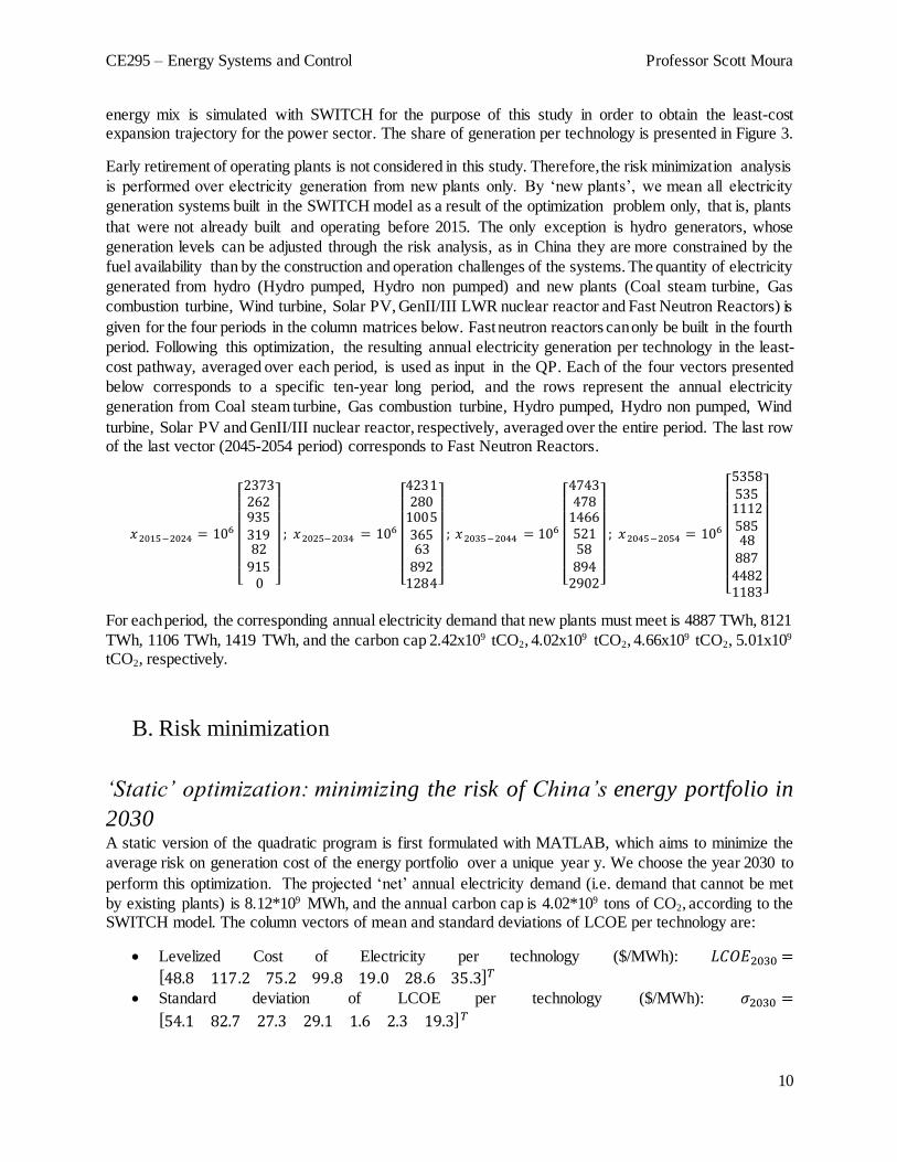
The SWITCH least-cost portfolio, Ps, characterized by 𝑥2025−2034, presents an average electricity
production cost of $52.12/MWh and a risk on this cost of $28.73/MWh. By allowing the generation level
from each technology to vary within plus and minus 10% around the least-cost generation levels, the QP
identifies least-risk energy portfolios, subject to the set of constraints presented in the previous section,
among all the possible combinations. Within a given range of costs, the set of corresponding portfolios with
lowest risks is called the efficient frontier. On Figure 4 below, the efficient frontier represents all the Pareto-
optimal portfolios whose costs range from $52.2/MWh to $53.3/MWh.
Figure 4 Efficient frontier of the 2030 energy portfolio options for average electricity cost between $52.2/MWh and $53.3/MWh
(QP optimization). The red cross gives the electricity cost and risk on the SWITCH least-cost portfolio. The generation share of
the eight energy system technologies are presented in the pie charts for P1, P2, P3 and the SWITCH portfolio.
Within the given range of costs, we distinguish three notables Pareto-optimal portfolios: P1, P2 and P3.
P1 is the least-cost portfolio, slightly higher – by less than $0.09/MWh - than the non-Pareto optimal least-
cost portfolio PS identified by SWITCH. P3 is the least-risk portfolio. Between P1 and P3, P2 is the portfolio presenting the highest decrease in risk per unit of increase in cost, it is the solution to:
min𝑃𝑖
|𝑅𝑖𝑠𝑘(𝑃𝑖)− 𝑅𝑖𝑠𝑘(𝑃𝑆)|− |𝐶𝑜𝑠𝑡(𝑃𝑖) − 𝐶𝑜𝑠𝑡(𝑃𝑆)|
27.5
27.7
27.9
28.1
28.3
28.5
28.7
28.9
52.2 52.3 52.4 52.5 52.6 52.7 52.8 52.9 53 53.1 53.2 53.3
Ris
k o
n c
ost
($/M
Wh
)
Electricity generation cost ($/MWh)
P1
P2
P3
Achievable region
PSWITCH
CE295 – Energy Systems and Control Professor Scott Moura
12
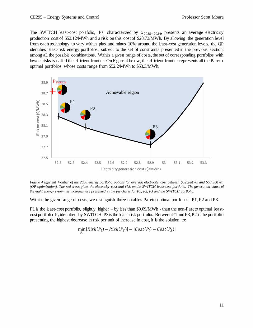
Figure 5 Sum of the changes in risks and in costs between the Pareto-optimal portfolios and the least-cost portfolio for different
costs. The dash line represents the tangent at the global maximum of the curve.
As can be seen on Figure 4, the optimal portfolios P1, P2 and P3 are similar in nature, as the generation
levels cannot differ from more than 10% around the SWITCH results. We notice, though, that P3 presents
a lower share of coal than P1. In the specific conditions used for this optimization, increasing the share of coal in the energy mix decreases its risk but increases its cost.
Figure 5 presents the sum of the change in risks (positive) and in costs (negative) between each of the
portfolios on the efficient frontier and the SWITCH portfolio. Portfolios corresponding to negative values
on this graph – costs higher than $53/MWh - are of little interest as their increase in costs compared with
the least-cost portfolio offsets their decrease in risks on costs. Actually, no portfolio whose cost is higher
than P3 - $52.9/MWh - should be considered as, for any of them, there exists a portfolio with same level of risk and lower costs, somewhere on the left branch of the frontier.
Portfolios showing a cost below $52.9/MWh have a positive value on the y-axis in Figure 5. On this graph,
the curve shows a global maximum at $52.4/MWh, corresponding to P2, with a positive difference in risks higher by $0.37/MWh than the negative difference in costs (in absolute terms).
Any of the portfolios between P1 and P3, including P2, could be favored by policy makers, depending on
their level of risk aversion, that is on how much they are willing to increase the costs from the least-cost portfolio in order to reduce the risks.
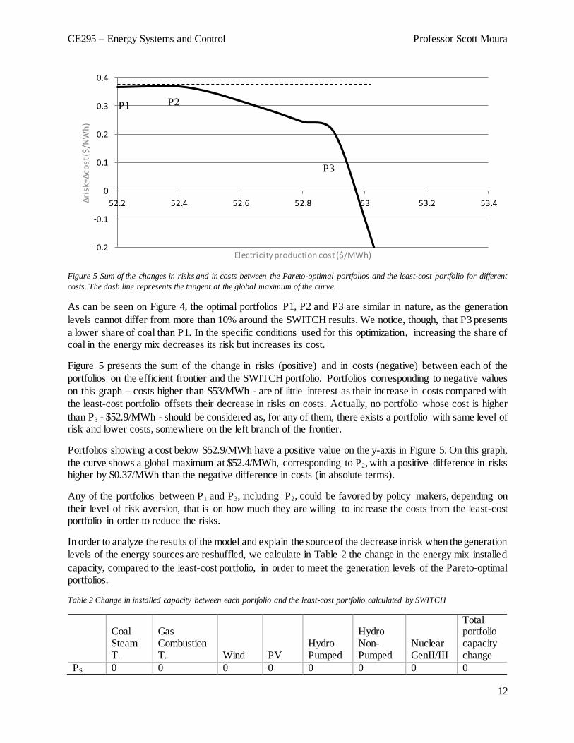
In order to analyze the results of the model and explain the source of the decrease in risk when the generation
levels of the energy sources are reshuffled, we calculate in Table 2 the change in the energy mix installed
capacity, compared to the least-cost portfolio, in order to meet the generation levels of the Pareto-optimal portfolios.
Table 2 Change in installed capacity between each portfolio and the least-cost portfolio calculated by SWITCH
Coal Steam T.
Gas Combustion T. Wind PV
Hydro Pumped
Hydro Non-Pumped
Nuclear GenII/III
Total portfolio capacity change
PS 0 0 0 0 0 0 0 0
-0.2
-0.1
0
0.1
0.2
0.3
0.4
52.2 52.4 52.6 52.8 53 53.2 53.4Δri
sk+Δ
cost
($/N
Wh
)
Electricity production cost ($/MWh)
P2 P1
P3
CE295 – Energy Systems and Control Professor Scott Moura
13
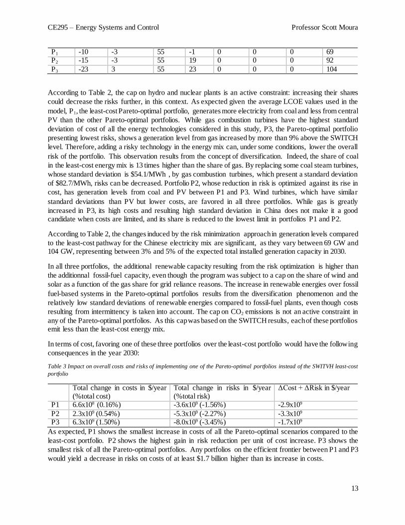
P1 -10 -3 55 -1 0 0 0 69 P2 -15 -3 55 19 0 0 0 92
P3 -23 3 55 23 0 0 0 104
According to Table 2, the cap on hydro and nuclear plants is an active constraint: increasing their shares
could decrease the risks further, in this context. As expected given the average LCOE values used in the
model, P1, the least-cost Pareto-optimal portfolio, generates more electricity from coal and less from central
PV than the other Pareto-optimal portfolios. While gas combustion turbines have the highest standard
deviation of cost of all the energy technologies considered in this study, P3, the Pareto-optimal portfolio
presenting lowest risks, shows a generation level from gas increased by more than 9% above the SWITCH
level. Therefore, adding a risky technology in the energy mix can, under some conditions, lower the overall
risk of the portfolio. This observation results from the concept of diversification. Indeed, the share of coal
in the least-cost energy mix is 13 times higher than the share of gas. By replacing some coal steam turbines,
whose standard deviation is $54.1/MWh , by gas combustion turbines, which present a standard deviation
of $82.7/MWh, risks can be decreased. Portfolio P2, whose reduction in risk is optimized against its rise in
cost, has generation levels from coal and PV between P1 and P3. Wind turbines, which have similar
standard deviations than PV but lower costs, are favored in all three portfolios. While gas is greatly
increased in P3, its high costs and resulting high standard deviation in China does not make it a good candidate when costs are limited, and its share is reduced to the lowest limit in portfolios P1 and P2.
According to Table 2, the changes induced by the risk minimization approach in generation levels compared
to the least-cost pathway for the Chinese electricity mix are significant, as they vary between 69 GW and 104 GW, representing between 3% and 5% of the expected total installed generation capacity in 2030.
In all three portfolios, the additional renewable capacity resulting from the risk optimization is higher than
the additionnal fossil-fuel capacity, even though the program was subject to a cap on the share of wind and
solar as a function of the gas share for grid reliance reasons. The increase in renewable energies over fossil
fuel-based systems in the Pareto-optimal portfolios results from the diversification phenomenon and the
relatively low standard deviations of renewable energies compared to fossil-fuel plants, even though costs
resulting from intermittency is taken into account. The cap on CO2 emissions is not an active constraint in
any of the Pareto-optimal portfolios. As this cap was based on the SWITCH results, each of these portfolios emit less than the least-cost energy mix.
In terms of cost, favoring one of these three portfolios over the least-cost portfolio would have the following
consequences in the year 2030:
Table 3 Impact on overall costs and risks of implementing one of the Pareto-optimal portfolios instead of the SWITVH least-cost
portfolio
Total change in costs in $/year (%total cost)
Total change in risks in $/year (%total risk)
ΔCost + ΔRisk in $/year
P1 6.6x10⁸ (0.16%) -3.6x10⁹ (-1.56%) -2.9x10⁹
P2 2.3x10⁹ (0.54%) -5.3x10⁹ (-2.27%) -3.3x10⁹ P3 6.3x10⁹ (1.50%) -8.0x10⁹ (-3.45%) -1.7x10⁹
As expected, P1 shows the smallest increase in costs of all the Pareto-optimal scenarios compared to the
least-cost portfolio. P2 shows the highest gain in risk reduction per unit of cost increase. P3 shows the
smallest risk of all the Pareto-optimal portfolios. Any portfolios on the efficient frontier between P1 and P3
would yield a decrease in risks on costs of at least $1.7 billion higher than its increase in costs.
CE295 – Energy Systems and Control Professor Scott Moura
14
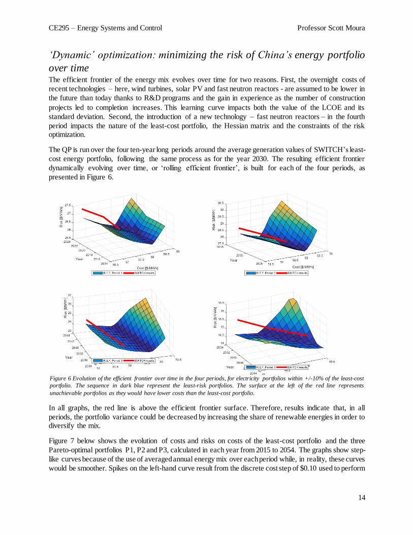
‘Dynamic’ optimization: minimizing the risk of China’s energy portfolio
over time The efficient frontier of the energy mix evolves over time for two reasons. First, the overnight costs of
recent technologies – here, wind turbines, solar PV and fast neutron reactors - are assumed to be lower in
the future than today thanks to R&D programs and the gain in experience as the number of construction
projects led to completion increases. This learning curve impacts both the value of the LCOE and its
standard deviation. Second, the introduction of a new technology – fast neutron reactors – in the fourth
period impacts the nature of the least-cost portfolio, the Hessian matrix and the constraints of the risk optimization.
The QP is run over the four ten-year long periods around the average generation values of SWITCH’s least-
cost energy portfolio, following the same process as for the year 2030. The resulting efficient frontier
dynamically evolving over time, or ‘rolling efficient frontier’, is built for each of the four periods, as
presented in Figure 6.
In all graphs, the red line is above the efficient frontier surface. Therefore, results indicate that, in all
periods, the portfolio variance could be decreased by increasing the share of renewable energies in order to diversify the mix.
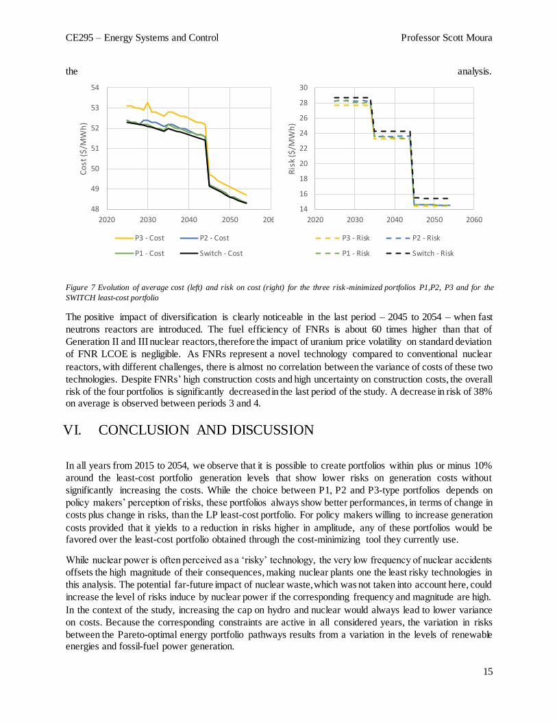
Figure 7 below shows the evolution of costs and risks on costs of the least-cost portfolio and the three
Pareto-optimal portfolios P1, P2 and P3, calculated in each year from 2015 to 2054. The graphs show step-
like curves because of the use of averaged annual energy mix over each period while, in reality, these curves
would be smoother. Spikes on the left-hand curve result from the discrete cost step of $0.10 used to perform
Figure 6 Evolution of the efficient frontier over time in the four periods, for electricity portfolios within +/-10% of the least-cost
portfolio. The sequence in dark blue represent the least-risk portfolios. The surface at the left of the red line represents
unachievable portfolios as they would have lower costs than the least-cost portfolio.
CE295 – Energy Systems and Control Professor Scott Moura
15
the analysis.
The positive impact of diversification is clearly noticeable in the last period – 2045 to 2054 – when fast
neutrons reactors are introduced. The fuel efficiency of FNRs is about 60 times higher than that of
Generation II and III nuclear reactors, therefore the impact of uranium price volatility on standard deviation
of FNR LCOE is negligible. As FNRs represent a novel technology compared to conventional nuclear
reactors, with different challenges, there is almost no correlation between the variance of costs of these two
technologies. Despite FNRs’ high construction costs and high uncertainty on construction costs, the overall
risk of the four portfolios is significantly decreased in the last period of the study. A decrease in risk of 38% on average is observed between periods 3 and 4.
VI. CONCLUSION AND DISCUSSION
In all years from 2015 to 2054, we observe that it is possible to create portfolios within plus or minus 10%
around the least-cost portfolio generation levels that show lower risks on generation costs without
significantly increasing the costs. While the choice between P1, P2 and P3-type portfolios depends on
policy makers’ perception of risks, these portfolios always show better performances, in terms of change in
costs plus change in risks, than the LP least-cost portfolio. For policy makers willing to increase generation
costs provided that it yields to a reduction in risks higher in amplitude, any of these portfolios would be favored over the least-cost portfolio obtained through the cost-minimizing tool they currently use.
While nuclear power is often perceived as a ‘risky’ technology, the very low frequency of nuclear accidents
offsets the high magnitude of their consequences, making nuclear plants one the least risky technologies in
this analysis. The potential far-future impact of nuclear waste, which was not taken into account here, could
increase the level of risks induce by nuclear power if the corresponding frequency and magnitude are high.
In the context of the study, increasing the cap on hydro and nuclear would always lead to lower variance
on costs. Because the corresponding constraints are active in all considered years, the variation in risks
between the Pareto-optimal energy portfolio pathways results from a variation in the levels of renewable energies and fossil-fuel power generation.
48
49
50
51
52
53
54
2020 2030 2040 2050 2060
Co
st (
$/M
Wh
)
P3 - Cost P2 - Cost
P1 - Cost Switch - Cost
14
16
18
20
22
24
26
28
30
2020 2030 2040 2050 2060
Ris
k ($
/MW
h)
P3 - Risk P2 - Risk
P1 - Risk Switch - Risk
Figure 7 Evolution of average cost (left) and risk on cost (right) for the three risk -minimized portfolios P1,P2, P3 and for the
SWITCH least-cost portfolio
CE295 – Energy Systems and Control Professor Scott Moura
16
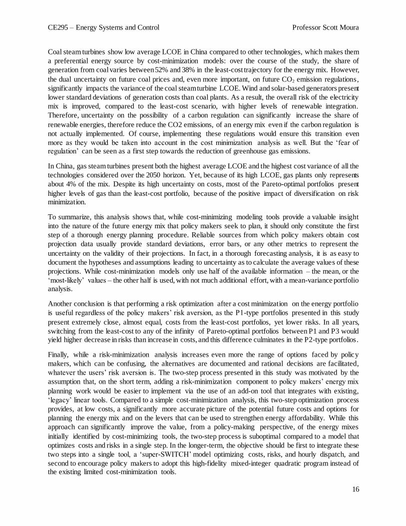
Coal steam turbines show low average LCOE in China compared to other technologies, which makes them
a preferential energy source by cost-minimization models: over the course of the study, the share of
generation from coal varies between 52% and 38% in the least-cost trajectory for the energy mix. However,
the dual uncertainty on future coal prices and, even more important, on future CO2 emission regulations,
significantly impacts the variance of the coal steam turbine LCOE. Wind and solar-based generators present
lower standard deviations of generation costs than coal plants. As a result, the overall risk of the electricity
mix is improved, compared to the least-cost scenario, with higher levels of renewable integration.
Therefore, uncertainty on the possibility of a carbon regulation can significantly increase the share of
renewable energies, therefore reduce the CO2 emissions, of an energy mix even if the carbon regulation is
not actually implemented. Of course, implementing these regulations would ensure this transition even
more as they would be taken into account in the cost minimization analysis as well. But the ‘fear of regulation’ can be seen as a first step towards the reduction of greenhouse gas emissions.
In China, gas steam turbines present both the highest average LCOE and the highest cost variance of all the
technologies considered over the 2050 horizon. Yet, because of its high LCOE, gas plants only represents
about 4% of the mix. Despite its high uncertainty on costs, most of the Pareto-optimal portfolios present
higher levels of gas than the least-cost portfolio, because of the positive impact of diversification on risk minimization.
To summarize, this analysis shows that, while cost-minimizing modeling tools provide a valuable insight
into the nature of the future energy mix that policy makers seek to plan, it should only constitute the first
step of a thorough energy planning procedure. Reliable sources from which policy makers obtain cost
projection data usually provide standard deviations, error bars, or any other metrics to represent the
uncertainty on the validity of their projections. In fact, in a thorough forecasting analysis, it is as easy to
document the hypotheses and assumptions leading to uncertainty as to calculate the average values of these
projections. While cost-minimization models only use half of the available information – the mean, or the
‘most-likely’ values – the other half is used, with not much additional effort, with a mean-variance portfolio analysis.
Another conclusion is that performing a risk optimization after a cost minimization on the energy portfolio
is useful regardless of the policy makers’ risk aversion, as the P1-type portfolios presented in this study
present extremely close, almost equal, costs from the least-cost portfolios, yet lower risks. In all years,
switching from the least-cost to any of the infinity of Pareto-optimal portfolios between P1 and P3 would yield higher decrease in risks than increase in costs, and this difference culminates in the P2-type portfolios.
Finally, while a risk-minimization analysis increases even more the range of options faced by policy
makers, which can be confusing, the alternatives are documented and rational decisions are facilitated,
whatever the users’ risk aversion is. The two-step process presented in this study was motivated by the
assumption that, on the short term, adding a risk-minimization component to policy makers’ energy mix
planning work would be easier to implement via the use of an add-on tool that integrates with existing,
‘legacy’ linear tools. Compared to a simple cost-minimization analysis, this two-step optimization process
provides, at low costs, a significantly more accurate picture of the potential future costs and options for
planning the energy mix and on the levers that can be used to strengthen energy affordability. While this
approach can significantly improve the value, from a policy-making perspective, of the energy mixes
initially identified by cost-minimizing tools, the two-step process is suboptimal compared to a model that
optimizes costs and risks in a single step. In the longer-term, the objective should be first to integrate these
two steps into a single tool, a ‘super-SWITCH’ model optimizing costs, risks, and hourly dispatch, and
second to encourage policy makers to adopt this high-fidelity mixed-integer quadratic program instead of the existing limited cost-minimization tools.
CE295 – Energy Systems and Control Professor Scott Moura
17
VII. REFERENCES
[1] International Energy Agency, “World Energy Outlook 2014,” 2014.
[2] International Energy Agency, “CO2 Emissions From Fuel Combustion - Highlights, ”
2014.
[3] F. Cavallaro, Assessment and simulation tools for sustainable energy systems: theory and applications. 2013.
[4] Bates White LLC., “A mean-variance portfolio optimization of california’s generation mix
to 2020: achieving california’s 33 percent renewable portfolio standard goal,” 2007.
[5] E. Worrell, S. Ramesohl, and G. Boyd, “Advances in Energy Forecasting Models Based on Engineering Economics*,” Annu. Rev. Environ. Resour., vol. 29, no. 1, pp. 345–381, 2004.
[6] L. Schrattenholzer, “Energy Planning Methodologies and Tools,” 2005.
[7] H. Version, “Getting Started Guide for HOMER Version 2.1,” 2005.
[8] S. E. Clark and T. T. Yates, “How efficient is your frontier?,” no. November, pp. 1–5,
2003.
[9] H. Markowitz, “Portfolio selection,” J. Finance, vol. 7, no. 1, pp. 77–91, 1952.
[10] D. G. Luenberger, Investment Science. 1998.
[11] Z. Bodie, A. Kane, and A. Marcus, Investments. 2004.
[12] E. Delarue, C. De Jonghe, R. Belmans, and W. D’haeseleer, “Applying portfolio theory to the electricity sector: Energy versus power,” Energy Econ., vol. 33, no. 1, pp. 12–23, 2011.
[13] F. Kienzle, G. Koeppel, P. Stricker, and G. Andersson, “Efficient electricity production
portfolios taking into account physical boundaries,” Methods, pp. 1–17.
[14] J. I. Muñoz, A. a. Sánchez de la Nieta, J. Contreras, and J. L. Bernal-Agustín, “Optimal investment portfolio in renewable energy: The Spanish case,” Energy Policy, vol. 37, pp. 5273–
5284, 2009.
[15] A. Bhattacharya and S. Kojima, “Power sector investment risk and renewable energy: A Japanese case study using portfolio risk optimization method,” Energy Policy, vol. 40, pp. 69–80, 2012.
[16] R. Salazar and M. Hutchison, “A mean-variance portfolio optimization of California’s
generation mix to 2020: achieving California’s 33 percent renewable portfolio,” 2007.
CE295 – Energy Systems and Control Professor Scott Moura
18
[17] L. Zhu and Y. Fan, “Optimization of China’s generating portfolio and policy implicat ions based on portfolio theory,” Energy, vol. 35, no. 3, pp. 1391–1402, 2010.
[18] C. Gao, M. Sun, B. Shen, R. Li, and L. Tian, “Optimization of China’s energy structure
based on portfolio theory,” Energy, vol. 77, pp. 890–897, 2014.
[19] G. He, A.-P. Avrin, J. H. Nelson, J. Johnston, A. Mileva, J. Tian, and D. M. Kammen, “Peaking Carbon in 2030? A Systems Approach to the Transition to a Sustainable Power System
in China,” Submitt. Publ., 2015.
[20] U.S. Energy Information Administration (EIA), “Levelized Cost and Levelized Avoided Cost of New Generation Resources in the Annual Energy Outlook 2014.” [Online]. Availab le :
http://www.eia.gov/forecasts/aeo/electricity_generation.cfm. [Accessed: 03-Mar-2015].
[21] J. C. Jansen, L. W. M. Beurskens, and X. van Tilburg, “Application of portfolio analysis to the Dutch generating mix Reference case and two renewables cases : year 2030 - SE and GE scenario,” no. February, pp. 5–67, 2006.
[22] D. Gotham, K. Muthuraman, P. Preckel, R. Rardin, and S. Ruangpattana, “A load factor based mean-variance analysis for fuel diversification,” Energy Econ., vol. 31, no. 2, pp. 249–256, 2009.
[23] Y.-H. Huang and J.-H. Wu, “A portfolio risk analysis on electricity supply planning, ”
Energy Policy, vol. 36, no. 2, pp. 627–641, 2008.
[24] M. Fripp, “Optimal Investment in Wind and Solar Power in California (Ph.D.),” Univers ity of California, Berkeley, United States, 2008.
[25] J. Nelson, J. Johnston, A. Mileva, M. Fripp, I. Hoffman, A. Petros-Good, C. Blanco, and
D. M. Kammen, “High-resolution modeling of the western North American power system demonstrates low-cost and low-carbon futures,” Energy Policy, vol. 43, pp. 436–447, Apr. 2012.
[26] A. Mileva, J. H. Nelson, J. Johnston, and D. M. Kammen, “SunShot solar power reduces
costs and uncertainty in future low-carbon electricity systems.,” Environ. Sci. Technol., vol. 47, no. 16, pp. 9053–60, Aug. 2013.
[27] M. Wei, J. H. Nelson, J. B. Greenblatt, A. Mileva, J. Johnston, M. Ting, C. Yang, C. Jones, J. E. McMahon, and D. M. Kammen, “Deep carbon reductions in California require electrifica t ion
and integration across economic sectors,” Environ. Res. Lett., vol. 8, no. 1, p. 014038, Mar. 2013.
[28] “U.S.-China Joint Announcement on Climate Change | The White House.” [Online]. Available: https://www.whitehouse.gov/the-press-office/2014/11/11/us-china-joint-
announcement-climate-change. [Accessed: 24-Apr-2015].
CE295 – Energy Systems and Control Professor Scott Moura
19
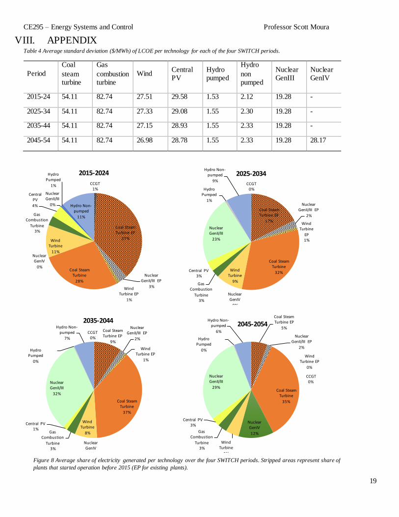
VIII. APPENDIX Table 4 Average standard deviation ($/MWh) of LCOE per technology for each of the four SWITCH periods.
Period
Coal
steam turbine
Gas
combustion turbine
Wind Central PV
Hydro pumped
Hydro
non pumped
Nuclear GenIII
Nuclear GenIV
2015-24 54.11 82.74 27.51 29.58 1.53 2.12 19.28 -
2025-34 54.11 82.74 27.33 29.08 1.55 2.30 19.28 -
2035-44 54.11 82.74 27.15 28.93 1.55 2.33 19.28 -
2045-54 54.11 82.74 26.98 28.78 1.55 2.33 19.28 28.17
CCGT0%
Coal Steam Turbine EP
17%
Nuclear GenII/III EP
2%
Wind Turbine
EP1%
Coal Steam Turbine
32%
Nuclear GenIV
0%
Wind Turbine
9%Gas
Combustion
Turbine3%
Central PV3%
Nuclear GenII/III
23%
Hydro Pumped
1%
Hydro Non-pumped
9%
2025-2034
CCGT0%
Coal Steam Turbine EP
9%
Nuclear GenII/III EP
2%
Wind Turbine EP
1%
Coal Steam Turbine
37%
Nuclear GenIV
0%
Wind Turbine
8%Gas Combustion
Turbine3%
Central PV1%
Nuclear GenII/III
32%
Hydro Pumped
0%
Hydro Non-pumped
7%
2035-2044
CCGT0%
Coal Steam Turbine EP
5%
Nuclear GenII/III EP
2%
Wind Turbine EP
0%
Coal Steam Turbine
35%
Nuclear GenIV
12%
Wind Turbine
5%
Gas Combustion
Turbine3%
Central PV3%
Nuclear GenII/III
29%
Hydro Pumped
0%
Hydro Non-pumped
6%
2045-2054
CCGT1%
Coal Steam Turbine EP
37%
Nuclear GenII/III EP
3%Wind Turbine EP
1%
Coal Steam Turbine
28%
Nuclear GenIV
0%
Wind Turbine
11%
Gas Combustion
Turbine3%
Central PV
4%
Nuclear GenII/III
0%
Hydro Pumped
1%
Hydro Non-pumped
11%
2015-2024
Figure 8 Average share of electricity generated per technology over the four SWITCH periods. Stripped areas represent share of
plants that started operation before 2015 (EP for existing plants).