B ENJAMIN H USTONS ANAA N ADEEM

I NCI O TKER-R OBE

Wo r k s h o p o n M o n e t a r y P o l i c y : S p i l l o v e r s a n d I n d e p e n d e n c e( D e c e m b e r 1 8 , 2 0 1 4 )

ACCOMMODATIVE MONETARY POLICY: BREATHING SPACE OR BREEDING RISKS FOR

EMERGING MARKETS? THE ROLE FOR MACROPRUDENTIAL POLICY

Outline

Motivation Questions we ask What we do? Contribution and Challenges Next steps

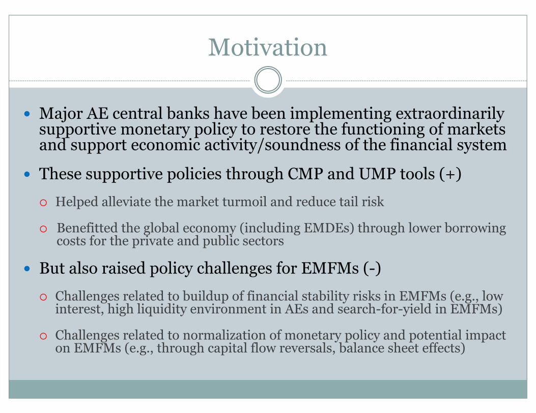
Motivation

Major AE central banks have been implementing extraordinarily supportive monetary policy to restore the functioning of markets and support economic activity/soundness of the financial system

These supportive policies through CMP and UMP tools (+)

Helped alleviate the market turmoil and reduce tail risk

Benefitted the global economy (including EMDEs) through lower borrowing costs for the private and public sectors

But also raised policy challenges for EMFMs (-)

Challenges related to buildup of financial stability risks in EMFMs (e.g., low interest, high liquidity environment in AEs and search-for-yield in EMFMs)

Challenges related to normalization of monetary policy and potential impact on EMFMs (e.g., through capital flow reversals, balance sheet effects)

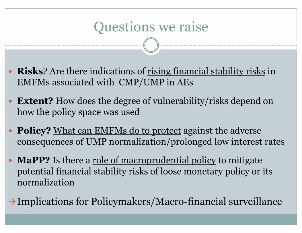
Questions we raise

Risks? Are there indications of rising financial stability risks in EMFMs associated with CMP/UMP in AEs

Extent? How does the degree of vulnerability/risks depend on how the policy space was used

Policy? What can EMFMs do to protect against the adverse consequences of UMP normalization/prolonged low interest rates

MaPP? Is there a role of macroprudential policy to mitigate potential financial stability risks of loose monetary policy or its normalization

Implications for Policymakers/Macro-financial surveillance

What we aim to do (1)

Consider the transmission channels of AE monetary policy to EMFMs

Examine correlations of AE interest rates with EMFM short and long-term interest rates, ERs, equity/house prices, capital inflows, credit growth…

Control for EMFM’s macro-financial characteristics and policy frameworks (e.g., degree of financial openness, ER regime, capital account openness…)

Derive estimates of EMFM financial cycles

Explore co-movements/correlations across financial cycles (between AE and EM cycles) and between EMFM financial cycles and AE rates

Assess the indication of rising financial risks in EMFMs based on the position in the financial cycle

For a sample of ~40 EMFMs

What we aim to do (2)

Assess how EMFMs used the supportive monetary policy space (indicators before/after UMP)—stylized facts To address macro and financial imbalances? To enhance financial/macro resilience and build policy space? or To build leverage/expand credit to nonproductive sectors?

Go more granular into the likely sources of financial risks (credit, FX, liquidity, etc)—key FSIs

Map the risks to MaPP tools to address the buildup of different risks, as well as to insure against adverse consequences for EMFMs of AE exit

Contributions, challenges, next steps

Key Contributions:

The angle to look into the role of MaPP in mitigating emerging financial risks and mapping the tools to risks for the sample EMFMs

Generation of financial cycles for EMDEs

Analyzing evolution and correlations across financial cycles

Key Challenges:

Generation of financial cycles for EMDEs—Absence of long data series for the key components of financial cycles

Innovation is to use imputation technique to derive the underlying data series to compute the financial cycles

Next steps: Preliminary draft around Spring 2015

Channels of Transmission—Example

Rolling correlations of EM ST rates with AE rates

Rolling correlations of EM LT rates with AE rates

-1.00

-0.75

-0.50

-0.25

0.00

0.25

0.50

0.75

1.00

2005 2006 2007 2008 2009 2010 2011 2012 2013 2014

US EU Japan

EM rolling correlations - Long term interest rates

-1.00

-0.75

-0.50

-0.25

0.00

0.25

0.50

0.75

1.00

2005 2006 2007 2008 2009 2010 2011 2012 2013 2014

US EU Japan

EM rolling correlations - short term interest rates

Transmission channels controlling for ER regime

Correlations of short term rates Correlations of long term rates

0.00.10.20.30.40.50.60.70.80.91.0

2000-2006 2007-2009 2010-2014

Pegged Managed Floating

0.00.10.20.30.40.50.60.70.80.91.0

2000-2006 2007-2009 2010-2014

Pegged Managed Floating

Transmission channels controlling for financial openness (Correlations of EM short-term rates with AE rates)

-1.00

-0.80

-0.60

-0.40

-0.20

0.00

0.20

0.40

0.60

0.80

1.00

0.00 0.20 0.40 0.60 0.80 1.00 1.20 1.40 1.60 1.80 2.00

2000-20072008-2014

Financial Openness (percentage of GDP)

Replicating BIS Financial Cycles

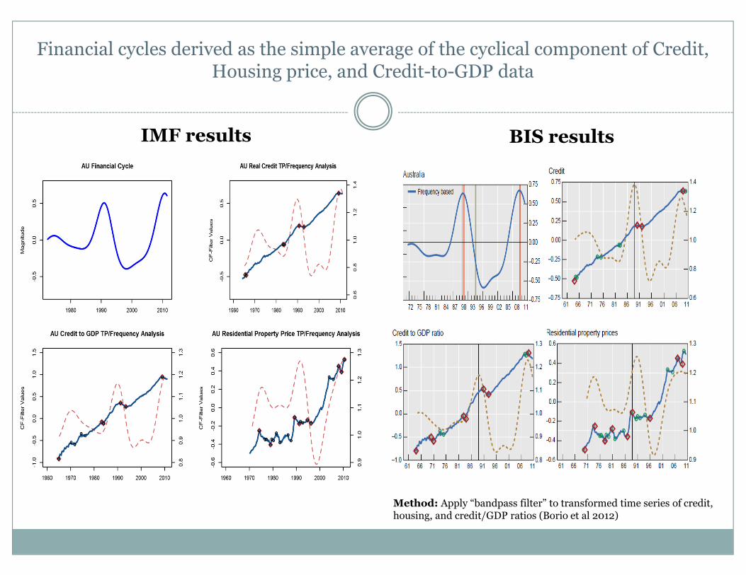
IMF results

Financial cycles derived as the simple average of the cyclical component of Credit, Housing price, and Credit-to-GDP data

BIS results

Method: Apply “bandpass filter” to transformed time series of credit, housing, and credit/GDP ratios (Borio et al 2012)

Two Approaches to Financial Cycles

Frequency Analysis Apply a “bandpass filter” to transformed time series of credit,

housing, and credit/gdp ratios Take the simple average of the cyclical component identified in these

three series to get the “financial cycle”

Turning Point Analysis Apply a modified version of the Bry and Boschan Quarterly

algorithm to transformed time series of credit, housing, and credit/GDP ratios to identify series-specific “peaks” and “troughs”

Pool series-specific peaks and troughs and repeat the process to identify “financial cycle” peaks and through.

*The Frequency Analysis approach is used almost exclusively in practice and its results are synonymous with the term financial cycle

Example: Advanced Economy Financial Cycles

Financial Cycle Interconnectivity

Illustrative Granger-Causality Network (1% significance level; 1985-2014)

The network of global financial cycles is highly connected

Exhibits high levels of “feedback” (mutual granger-causation) among advanced economies and between advanced and emerging economies

Addressing Data Constraints

The financial cycle imputation workflow17

Utilize iterated univariate procedures* (“chained equations”) that work in parallel to predict (“impute”) missing values of the response variable from previously observed response and predicator values

Use chained equations to impute missing data from observed data many times

Gather (incomplete) data

Perform subsequent analysis

Apply bandpassfilter to extract financial cycles from each imputed dataset

Pool results into a single financial cycles for each country

*van Buuren S, Brand JPL, Groothuis-Oudshoorn CGM, Rubin DB (2006b). “Fully Conditional Specification in Multivariate Imputation.” Journal of Statistical Computation and Simulation, 76(12), 1049–1064.

Experimental Imputed EM Housing Price Data

*Black line represents observed data. Red line represents data imputed usingchained equations.

Short imputation chain Long imputation chain

Appendix

The United Kingdom and the Euro Area are the most connected in the overall network

The closer a node is to the center the more “important”, as measured by betweeness centrality, the node is to the structure of the network,

Betweenness Centrality Graph of Granger-Causality Network (1% Significance Level; 1985-2014)

The U.S. and Korea are most similar in terms of in terms of connectivity.

The other countries (excluding Germany) have similar levels of connectivity.

Nodes groups denote “similarity”, as measured by betweenness centrality scores. Nodes within each group are most similar along this dimension.

Betweenness Community of Granger-Causality Network (1% Significance Level; 1985-2014)

A betweenness centrality-based cost function is used to determine “splits”

Partitions formed by splits represent distinct "communities”

First Split

Second Split

Betweenness Community Dendogram of Granger-Causality Network (1% Significance Level; 1985-2014)