access to credit and the size of the formal sector in brazil
TRANSCRIPT

Access to Credit and the Size of the Formal Sector in Brazil
Pablo N. D'Erasmo
Department of Research and Chief Economist
IDB-WP-404IDB WORKING PAPER SERIES No.
Inter-American Development Bank
April 2013

Access to Credit and the Size of the Formal Sector in Brazil
Pablo N. D'Erasmo
University of Maryland
2013
Inter-American Development Bank

http://www.iadb.org The opinions expressed in this publication are those of the authors and do not necessarily reflect the views of the Inter-American Development Bank, its Board of Directors, or the countries they represent.
The unauthorized commercial use of Bank documents is prohibited and may be punishable under the
Bank's policies and/or applicable laws.
Copyright © Inter-American Development Bank. This working paper may be reproduced for any non-commercial purpose. It may also be reproduced in any academic journal indexed by the American Economic Association's EconLit, with previous consent by the Inter-American Development Bank (IDB), provided that the IDB is credited and that the author(s) receive no income from the publication.
Cataloging-in-Publication data provided by the Inter-American Development Bank Felipe Herrera Library D'Erasmo, Pablo N. Access to credit and the size of the formal sector in Brazil / Pablo N. D'Erasmo. p. cm. (IDB working paper series ; 404) Includes bibliographical references. 1. Credit—Brazil. 2. Informal sector (Economics)—Brazil. 3. Microfinance—Brazil. I. Inter-American Development Bank. Research Dept. II. Title. III. Series. IDB-WP-404
2013

Abstract
This paper studies the link between credit conditions and formalization in Brazil, as bothcredit and the rate of formalization have notably increasedin the last decade. A firmdynamics model with endogenous formal and informal sectorsis developed to quanti-tatively evaluate how much of the change in corporate creditand the size of the formalsector can be attributed to a reduction in the cost of financial intermediation. The modelpredicts that the observed reduction in intermediation costs generates an increase in thecredit-to-output ratio and in the share of formal workers, in line with the data. It is foundthat—by affecting the corporate interest rate, the allocation of capital and the entry andexit rates—the change in credit conditions has important effects on firm size distributionand aggregate productivity1.
Keywords: Financial Structure, Informal Sector, Productivity.
JEL Classification: D24, E26, L11, O16, O17
1 This research was supported by the IDB. I would like to thank Kala Krishna, Veronica Frisancho Robles and EduardoCavallo for their valuable comments.

1 Introduction
This paper analyzes the link between credit conditions, thelevel of formalization and firm size dis-
tribution. Formalization in Brazil has risen by 21.69 percent since 2001 (from 45.5 percent to 55.37
percent.2 During the same period, due to favorable international liquidity and a decline in policy con-
trolled interest rates, there has been an improvement in credit conditions for Brazilian firms, evident
in the sharp increase in credit to firms over GDP (from 15 percent in 2003 to more than 22 percent in
2008) and a reduction in average interest rates charged on corporate loans.
The Brazilian experience is of particular interest becauseBrazil is among only a handful of
major emerging economies that saw bank lending double (as a share of GDP) during the last decade.
Together with structural reforms in the financial sector aimed to reduce the cost of corporate credit
and improved access to credit by financial institutions, a period of sound macroeconomic policies
contributed to the increase in credit and formalization.3 For example, during the administrations
of President Lula (2003-2010), inflation rates remained low, the government ran a primary surplus
on average of 3-4 percent of GDP, net public debt declined steadily, demand for Brazil’s exports
was strong and large gains occurred in the terms of trade. Theaim of this paper is to develop a
parsimonious model to study how the increased efficiency of financial institutions and the reduction
in their funding costs that resulted from structural reforms, as well as good macroeconomic conditions
and credit environment, affected aggregate credit and the rate of formalization.
More specifically, we ask what is the change in the level of corporate credit to GDP and for-
malization that can be attributed to improvements in the efficiency of financial intermediaries and a
reduction in their cost of funding. We answer this question by developing a general equilibrium model
of firm dynamics with endogenous entry and exit that incorporates capital financing and bankruptcy
decisions. The model allows for the existence of a formal andan informal sector. Entering and oper-
ating in the formal sector is costly but allows firms to accesscredit markets with better commitment
and greater efficiency. Financial intermediaries have access to international markets at a risk-free rate
but incur a proportional cost when issuing debt. The degree of debt enforcement affects the interest
rate that non-financial firms face because there is equilibrium default.
Our quantitative experiment proceeds as follows. We first calibrate a steady state of the model
using firm-level data and other relevant aggregate statistics from Brazil in the early 2000s.4 We also
use country-specific institutions based on those reported by the World Bank in itsDoing Business
database. This calibration allows us to pin down technologyparameters for non-financial firms and
financial intermediaries and determines the benchmark sizeof the informal sector, the level of credit
2 The definition of the formal sector is based on the share of workers who contribute to social security as in Catao, Pagesand Rosales (2009).3 The paper documents the structural reforms and the changes in credit conditions in the following section.4 The data from Brazil include the firm-level survey RAIS, a survey with informal firms ECINF, household survey anddetailed information on credit terms to the corporate sector as well as aggregates from different sources. The data andtheir sources are presented in the following section and in the Data Appendix that accompanies this paper.
2

and corporate spreads in the economy. Once the model is calibrated, we study the effect of a 37
percent reduction in the cost of funds for financial intermediaries (from 7.5 percent to 4.7 percent)
and a 44 percent reduction in the cost of issuing loans (from 5.58 percent to 3.31 percent). These
changes are calibrated using Brazilian data from 2003 to 2010 to match the observed reduction in the
money market interest rate and overhead costs for financial firms.
The reduction in intermediation costs produces an endogenous response in the level of credit,
the firm size distribution and the degree of formalization that is at the center of our paper. More
specifically, we find that a reduction in credit costs generates an increase in credit to GDP of approx-
imately 87 percent. The increase in the formal labor force is45 percent, therefore, as in the data, the
model generates sizable increases in the level of credit andthe size of the formal sector. An increase
in the level of formalization and the better allocation of resources allows the model to generate an in-
crease in measured aggregate TFP of approximately 15 percent and weighted firm-level productivity
of about 16 percent.
The intuition for these results is as follows. Changes in intermediation costs have a first order
effect on corporate bond prices. This translates into lowerdefault probabilities that in turn increase
bond prices even further (the loan spread endogenously decreases by 21.96 percent in the model).
This affects firm size distribution through the following channels. First, it induces incumbent firms to
change the composition of debt and capital. When interest rates are low, firms’ precautionary motive
for capital accumulation is reduced and incentives to borrow are stronger. Since firms do not face the
need to accumulate capital in order to survive adverse shocks, this increases efficiency in the economy
(i.e., firms move closer to their optimal level of capital). Second, it affects the endogenous entry and
exit productivity thresholds. Since the value of the firm is higher, it lowers the entry threshold into
formalization, increasing the fraction of output producedby formal firms. This affects productivity
in different directions. On one hand, lower entry thresholdhas a negative impact on the average level
of productivity of the entrant firm. On the other hand, a larger fraction of output is produced by
more productive formal firms. Finally, higher entry also results in stronger competition and higher
wages (due to higher aggregate demand for labor) that translates into more exit (with a positive effect
on productivity) and a reduction in the average size of the firm. We find that the positive effects on
productivity dominate and an increase in aggregate TFP is observed.
To understand the overall results even further, we also analyze one by one the effect of changes
in the cost of funds for financial intermediaries and the reduction in the cost of issuing loans. We find
that most of the effect on the level of credit is coming from the increase in the level of efficiency of the
financial sector (as opposed to changes in their funding costs). Moreover, we uncover an important
interaction effect between the level of efficiency and the cost of funds for intermediaries that allows
the model to generate the overall change in the size of the formal sector.
Our approach to firm dynamics started with Hopenhayn (1992) and Hopenhayn and Rogerson
(1993), and is close to Cooley and Quadrini (2001) who studied the effects of financial constraints
3
in a similar set-up. The modeling assumptions regarding theinformal sector follow the steps of
Rauch (1991) and Loayza (1996) where informal activity can be thought of as an optimal response to
the economic environment. The treatment of informality andcredit frictions follows D’Erasmo and
Moscoso Boedo (2012) and D’Erasmo, Moscoso Boedo and Senkal(2012). A related literature on the
distributional consequences of frictions in this context started with Restuccia and Rogerson (2008).
Important references are Hsieh and Klenow (2009), Guner, Ventura, and Xu (2008), Arellano, Bai,
and Zhang (2010) and Buera, Kaboski and Shin (2011). This paper introduces imperfect capital
markets, and along that dimension the most closely related papers include Antunes and Cavalcanti
(2007) and Quintin (2008).5 This paper builds upon this literature by analyzing to what extent the
observed changes in credit conditions in Brazil can generate the pattern that aggregate credit and the
size of the informal sector display.
The relevant empirical literature regarding firm dynamics across countries include Tybout
(2000), La Porta and Shleifer (2008), Foster, Haltiwanger,and Krizan (2001), Bartelsman, Halti-
wanger and Scarpetta (2009), and Alfaro, Charlton, and Kanczuk (2009). Tybout (2000) and La Porta
and Shleifer (2008) are the only ones that report data on firm characteristics in the informal sector,
while the other three use different data sources but are focused on firms operating in the formal sector.
The paper is organized as follows. Section 2 presents the relevant facts about the evolution of
formality and credit in Brazil during the last decade. Section 3 and 4 present the theoretical model
and its equilibrium. Section 5 is devoted to the calibrationof the model to the Brazilian data. Section
6 presents the main experiment. Finally, Section 7 concludes.
2 Credit, Formalization and Institutions in Brazil
This section describes the main facts driving our quantitative exercise. A description of the insti-
tutional framework and the changes in credit conditions is followed by an analysis of the firm size
distribution and the size of the informal sector. Finally, we describe a set of measured institutions that
are also important for understanding the link between credit imperfections, informality and produc-
tivity.
2.1 Institutional Reforms and Credit Conditions
The role of institutions such as the bankruptcy law shaping economic outcomes has been studied
extensively in the empirical literature (see, for example,La Porta et al., 1998, Djankov et al., 2008, and
Levine, 1999). The evidence points towards the importance of creditor rights. Developing economies
are characterized by lower legal protection of creditor rights as well as inefficient credit markets,
and until the early 2000s Brazil was no exception. However, several structural reforms (such as the
bankruptcy reform and decline in policy-controlled interest rates) together with favorable international
5 Antunes and Cavalcanti (2007) and Quintin (2008) study endogenous informal sectors that result from imperfect contractenforcement. Also related, Castro, Clementi and MacDonald(2008) and Erosa and Hidalgo Cabrillana (2008) study theeffects of financial contracts in environments with asymmetric information.
4

liquidity conditions, propelled the increase in corporatecredit, especially bank lending, observed
during the last decade.
The reforms implemented during this period contributed to the improvement in intermediation
efficiency and a large reduction in the cost of credit for non-financial and financial corporations in
Brazil. Although many emerging economies experienced rapid credit growth, the experience of Brazil
is of particular interest because Brazil is among only a handful of major emerging economies that saw
bank lending double (as a share of GDP) from 2000 to 2010.
One of the major changes in the institutional environment during the last decade was the
change in the Brazilian Bankruptcy Law that provided a significant increase in protection to creditors.
The old bankruptcy code in Brazil was enacted in 1945 and had remained largely unchanged until the
2005 bankruptcy law was enacted. Before the reform, creditors had a very low level of protection in
Brazil. This characteristic raised the interest rate spread and inhibited the supply of credit. The new
bankruptcy law encourages reorganization of claims in a bankrupt entity. In the event of liquidation,
the new law rearranges the absolute priority rules in favor of secured creditors. Before the reform,
bankruptcies in Brazil took on average 10 years to be resolved, which is roughly three times longer
than the time taken in the United States (3 years) and in the Latin American and Caribbean region
(3.6 years). This long bankruptcy resolution period reduced the time value of assets and led to greater
attrition through depreciation in the value of fixed assets.In summary, the new law provided major
protection to creditors and the focus was the improvement ofefficiency of the bankruptcy process.6
Another important set of financial reforms resulted from a number of bank failures during
the late 1990s. As Ter-Minassian (2012) describes, two major programs were implemented: one for
private banks (PROER) and another for public banks (PROES).The PROER program provided liq-
uidity to banks in difficulty but assessed to be ultimately solvent. The government provided financial
support for the acquisition of failing but salvageable banks and for an orderly unwinding of insolvent
ones, created a deposit guarantee fund. The Central Bank acquired powers of supervision and bank
resolution. The PROES program mainly focused on closing or privatizing public banks that were not
profitable. These programs were fundamental for the increase in efficiency observed in the financial
sector in Brazil for the years that followed.
The financial reforms during the last decade also include theimprovement of the legislation
regulating the realization of collateral for non-performing loans and the liberalization of entry by
foreign banks. This increased the level of competition in the financial sector (even though the system
remains dominated by relatively few large private and public banks) and drove down credit costs for
market participants.
6 Several major changes that affected the relation between firms and creditors were introduced as part of the newbankruptcy law. For example, secured and unsecured creditsare now given priority over tax credits, the distressed firmmight be sold (preferably as a whole) before the creditors list is compiled–which speeds up the process and increases firmvalue–and any new credit extended during the reorganization process is given first priority in the even of liquidation. SeeAraujo, Ferreira and Funchal (2012) for an exhaustive description of the new bankruptcy law in Brazil.
5
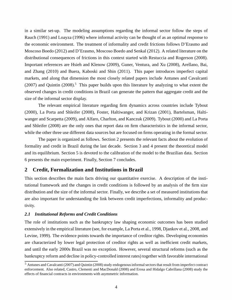
Figure 1. The Cost of Credit
2000 2002 2004 2006 2008 2010 20121
2
3
4
5
6
7
Year
Net Interest Margin
(%)
Note: Net Interest Margin corresponds to the difference between the average lending rate and the averagedeposit rate. Source Beck and Asli Demirguc-Kunt (2009) updated in 2012.
The set of financial reforms we described were accompanied bylow inflation rates and strong
demand for Brazil’s exports due to the large gains in the terms of trade observed in this period. These
factors also contributed to a better credit environment in general.
The reduction in intermediation costs were translated intoa lower cost of credit for non-
financial corporations. We obtained information on the costof credit from the data on financial
structure compiled by Thorsten Beck and Asli Demirguc-Kunt.7 We start with the evolution of the
interest rate margin (i.e., the difference between the average lending rate and the average deposit rate).
Figure 1 shows the reduction in the interest rate margin during 2000-2010.8
The figure shows that the reduction in the net interest marginwas of more than 75 percent from
its peak in 2003 (from 6.43 percent in 2002 to 1.66 percent in 2010) and that there is a significant drop
in 2005, the year when the new bankruptcy law was implemented.
Another observable measure of the changes in the structure of the financial sector and the
cost of funds for financial intermediaries is the sharp decrease in the real money market interest rate
during this period (see Figure 2).9 We collected data on the nominal money market interest rate
and transformed it into real using the consumer price index.Both series are from the International
Financial Statistics (IFS).
7 See the New Data version (2012) of the data originally provided in Beck and Asli Demirguc-Kunt (2009).8 See the Data Appendix for sources and definitions as well as a file that contains the data used.9 The money market corresponds basically to short-term fundsavailable to banks in everyday operations.
6

Figure 2. Intermediation Costs
2000 2002 2004 2006 2008 2010 2012
4
6
8
10
12
Year
(%)
Panel (i): Money Market Rate
2000 2002 2004 2006 2008 20102
3
4
5
6
7
Year
Panel (ii): Bank′s Overhead Costs (as fraction of assets)
(%)
Note: Money Market Interest Rate from IFS data. Overhead costs as a fraction of assets in the financial sectorfrom Financial Structure (2012) data.
7

Figure 3. Corporate Loan Interest Rates
2002 2003 2004 2005 2006 2007 2008 2009 2010 201110
11
12
13
14
15
16
17
Year
Bank Loan Interest Rates
(%)
AvgMedian
2002 2003 2004 2005 2006 2007 2008 2009 2010 20117
8
9
10
11
12Dispersion Bank Loan Interest Rates (std)
Year
(%)
Source: Brazilian Central Bank (SCR: Sistema de Informacoes de Credito do Banco Central)
Panel(i) of Figure 2 shows that the cost of funds for the financial sector in Brazil was reduced
by almost half in less than 10 years (from approximately 10 percent in 2000 to less than 5 percent
in 2010). Another important factor affecting the cost of credit for non-financial corporation is the
efficiency level in the financial sector. Panel(ii) of Figure 2 provides additional evidence on the
reduction in the cost of accessing credit. This figure presents data on bank overhead costs as a fraction
of total assets.These data come from Beck and Demirguc-Kunt (2009). We observe that overhead
costs decreased by 47 percent since the year 2000.
We obtained access to central bank data on bank credit on banklending to individual firms
(Sistema de Informacoes de Credito do Banco Central). These data contain very valuable information
on loan interest rates and lending amounts at the firm level reported directly from financial institu-
tions.10 Figure 3 presents the average, the median and the standard deviation of real loan interest
rates.11
10 These data are not publicly available. I thank Luis Catao, who provided the data, for allowing me to present this set ofsummary statistics. These statistics are included in a file that accompanies the Appendix.11 All measures presented correspond to loan-weighted measures. To avoid distortions caused by a few outliers, werestrict the sample to+/− 2 standard deviations of the original weighted mean.
8

Figure 4. Distribution of Corporate Loan Interest Rates
0 2 4 6 8 10 120
10
20
30
40
50
60
Loan Interest Rate (%)
Distribution Bank Loan Interest Rates
cdf (
%)
year 2004year 2007year 2010
Source: Brazilian Central Bank (SCR: Sistema de Informacoes de Credito do Banco Central)
These data do not show a clear pattern, as do those presented in Figure 1; however,
we observe that the average and the median interest rate to corporations decrease after their peak in
2004/2005. Consistent with the aggregate data, the reduction in interest rates is approximately 18
percent for the average and 25 percent for the median. The standard deviation is a useful summary
statistic of the dispersion of the observed interest rate distribution and allows us to infer the extent to
which financial intermediaries are expanding credit to those at the low end and the high end of the
distribution; there seems to be an increase in dispersion during this period. To present more evidence
on the change in interest rates, Figure 4 shows the entire distribution for selected years.
We note the increase in the weights on low interest rates whenmoving from year 2004 to year
2010. For example, year 2010 has approximately 40 percent ofthe total amount loaned below interest
rates of 6 percent, while for year 2004 at the same interest rate the corresponding fraction is around
20 percent.
Together with the reduction in intermediation costs and interest rates, there is a large expan-
sion in credit in Brazil during this period. Funchal and Clovis (2008) find evidence that the use of
bank debt increased significantly in the post-bankruptcy reform Brazilian market. Figure 5 presents
data consistent with this empirical finding. This figure shows the evolution of total domestic bank
9

Figure 5. The Evolution of Credit
2000 2002 2004 2006 2008 2010
15
20
25
30
35
40
Year
(%)
Credit in Brazil
Total CreditCorporate Credit
Source: Catao, Pages and Rosales (2009).
credit and domestic bank credit to the corporate sector to GDP, two traditional measures of financial
deepening.
Figure 5 shows that the ratio of overall credit to the privatesector (i.e., including credit to both
firms and households) relative to GDP rose dramatically in the period we are analyzing. Credit to
the corporate sector experienced a similar expansion, going from 15 percent in 2000 to 24 percent in
2010 (an increase of 58.7 percent).
Before moving into data on informality and then to the model,we would like to provide
more information on the link between financial reforms, credit conditions and credit at the firm level.
Araujo, Ferreira and Funchal (2012) present evidence on theconsequences of the bankruptcy reform.
They use a differences-in-differences approach to analyzethis event. More specifically, they compare
Brazilian firms (the treatment group) to non-Brazilian firmsfrom Argentina, Chile and Mexico (the
control group) with respect to the behavior of debt related variables.12 The source of their data is
Economatica, which includes 698 publicly traded firms from 1999 to 2009 (no financial institutions).
Of those firms, 338 are Brazilian (the treatment group), and the rest belong to the control group.
Table 1 presents their main results. As shown in Table 1, the authors find that the bankruptcy reform
generated a considerable increase in the total amount of debt at the firm level as well as a significant
12 They allow for different firm trends within treatment and control groups to account for the fact that the standarddifference-in-difference approach may not consistnetly estimate the average treatment effect due to the assumption ofcommon trends.
10

Table 1. Effects of the Bankruptcy Reform
Dep. VariableTotal Debt Cost Debt
Bankruptcy reform 0.1780 -0.1678s.e. 0.0640 0.0040Other Controls Yes YesObservations 3143 2487R2 0.09 0.03
Note: Source is Table 2 in Araujo, Ferreira and Funchal (2012). Differences in Difference estimation.Bankruptcy reform dummy takes value one after year 2004. Other controls include Taxes to Total Revenue,
Total Assets, Return on Assets, Price-to-Book ratio, Earnings before taxes. The source of the data isEconomatica. 698 publicly traded firms from 1999 to 2009 (no financial institutions). 338 firms are Brazilian
(the treatment group) and the rest to the control group.
reduction in the cost of credit. More specifically, the estimates indicate that the new bankruptcy
legislation generates an increase of 17.8 percent in total debt and a reduction of approximately 16.78
percent in the cost of debt.
2.2 Formalization and Firm Size Distribution
How does the change in credit conditions affect firm size distribution in Brazil? Credit markets
allow for a better allocation of resources. When credit markets improve, capital and labor move
closer to the efficient level. An important margin affectingresource misallocation is the level of
formalization in the economy. One of the main benefits of formalization is better access to credit,
since operating in the formal sector increases access to courts and other types of contract-enforcement
mechanisms, and financial institutions are generally not willing to extend loans to firms that lack the
proper documentation. Changes in the cost of funds affect not only existing firms by allowing them to
expand or to survive larger adverse shocks, but also the number and the size of those firms that decide
to start operating in the formal sector. This has important implications, since it affects the dynamics
of firm size distribution.
In fact, a dramatic change in the level of formalization was observed in Brazil during this
period. Using data from the Brazilian National Institute ofGeography and Statistics (IBGE), we
present the share of formal workers in the economy (measuredas the share of workers that contribute
to Social Security). Figure 6 shows that the share of formal workers has increased by more than 21
percent (from 45 percent in 2001 to 55 percent in 2010).
Evidence on the credit channel was also presented in Catao,Pages and Rosales (2009). They
used a difference-in-difference approach applied to household survey data from Brazil to show that
11

Figure 6. Level of Formalization
2000 2002 2004 2006 2008 201040
42
44
46
48
50
52
54
56
58
60
Year
(%)
Size Formal Sector
Source: Brazilian National Institute of Geography and Statistics (IBGE).
formalization rates increase with financial deepening , especially in sector where firms are typically
more dependent on external finance.13
The relation between credit and the level of formalization has important effects for the firm
size distribution because informal firms tend to be much smaller and unproductive that formal firms.
To shed light on the firm size distribution we use two data sources. The first source is the ECINF
survey (Pesquisa de Economia Informal Urbana), a representative cross-section of small firms (with
at most five employees) collected at the national level by theBrazilian Bureau of Statistics (IBGE) in
2003.14,15 The second source is the universe of formal firms, RAIS (Relacao Anual de Informacoes
Sociais), compiled by the Brazilian Ministry of Labor which requiresby law that all formally regis-
tered firms report information each year on each worker employed by the firm.16
From the ECINF, we can take a close look at the “Micro-Sector”in Brazil. Table 2 presents
the distribution of firms with fiver or less workers. This includes formal and informal firms. Table 213 The measure of external finance is the standard Rajan-Zingales (1998) index.14 ECINF samples households located in urban areas and seeks toidentify the self-employed and em-ployers with up to five employees in at least one work situation. This data set has been used in re-cent studies by Fajnzylber, Maloney and Montes-Rojas (2011) and Ulyssea (2012), for example. Seehttp://www.ibge.gov.br/home/estatistica/economia/ecinf/2003/default.shtm for more information.15 The ECINF offers extensive detail on the main firm and the entrepreneur characteristics of microenterprises such assector revenues, profits employment size, capital stock andtime in business.16 In both cases, ECINF and RAIS, we only have access to aggregate information provided in a large set of tables by theoriginal source. See the Data Appendix for a full description of variables used and links to corresponding tables.
12

Table 2. “Micro-Sector” Firm Size Distribution
“Micro-Sector” Size Distribution# of Workers Fraction of Firms % CDF %0 86.60 86.601 7.40 94.002−3 4.60 98.604−5 1.40 100.00
Note: “Micro-Sector” defined as firms with 5 or less employees. Source is ECINF survey, arepresentative cross-section of small firms (5 or less employees) collected at the national level.
shows that when we look at both formal and informal firms, a considerable mass is allocated in the
small bins. More than 80 percent of firms employ no workers, and almost 95 percent employ less than
1 worker.
Using the ECINF and RAIS, we can look at the differences between formal and informal
firm size distribution. Table 3 presents formal size distribution from RAIS (i.e., the distribution of
registered firms) and informal size distribution from ECINF(i.e., the distribution of unregistered
firms). As shown in Table 3, most informal firms employ less than three workers (98.23 percent), the
first bin in the distribution of formal firms. IBGE identified 10,525,954 small enterprises in Brazil in
2003, and 98 percent of them were defined as informal (not registered). A large share of formal firms
are also concentrated in the small size bins, but there is considerable dispersion in terms of workers
per plant/firm.
2.3 Measured Formal Institutions
Besides access to credit, institutions that affect the costof operating a formal firm are also important
determinants of the size of the formal sector and the level ofaggregate credit in the economy. These
include corporate taxes, entry costs into formalization and labor market costs such as payroll taxes
and firing costs. To obtain information on these institutions we use the World BankDoing Business
dataset. These data measure the costs, in terms of time and resources, along many dimensions affect-
ing the firm, such as starting a business, getting construction permits, employing workers, obtaining
credit, protecting investors, paying taxes, trading across borders, enforcing contracts, and closing a
business. Of particular interest are the cost of entering the formal sector, the profit tax rate, the payroll
tax rate, the efficiency of the bankruptcy law and firing costs.
We describe how these measured institutions are constructed:17
Entry Cost: The cost of entering the formal sector corresponds to the reported “costs of registering
17 We are interested in values reported in 2003, but we use values for the most recent year when the observation for2003 is not reported. Since these variables measure long-term institutional arrangements, not having the informationfora particular year does not bias the estimates to a large extent.
13
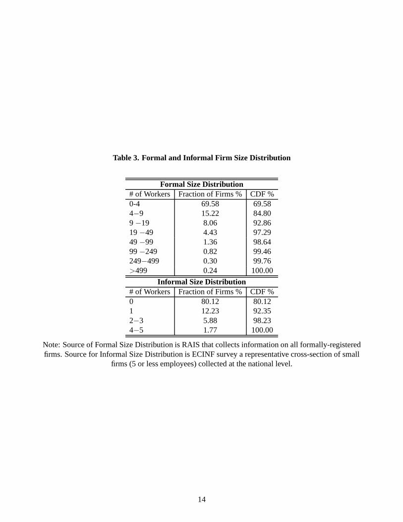
Table 3. Formal and Informal Firm Size Distribution
Formal Size Distribution# of Workers Fraction of Firms % CDF %0-4 69.58 69.584−9 15.22 84.809 −19 8.06 92.8619−49 4.43 97.2949−99 1.36 98.6499−249 0.82 99.46249−499 0.30 99.76>499 0.24 100.00
Informal Size Distribution# of Workers Fraction of Firms % CDF %0 80.12 80.121 12.23 92.352−3 5.88 98.234−5 1.77 100.00
Note: Source of Formal Size Distribution is RAIS that collects information on all formally-registeredfirms. Source for Informal Size Distribution is ECINF surveya representative cross-section of small
firms (5 or less employees) collected at the national level.
14

a business and of dealing with licenses to operate a physicallocale.” It involves the cost of starting a
business as a share of income per capita. The estimate of the entry cost for Brazil is 0.739 of GNI per
capita.
Taxes:The tax rate paid on profits by the firms is taken from “Paying Taxes - Profit tax (%)”
and the payroll tax corresponds to “Paying Taxes - Labor tax and contributions (%).”18 The estimated
values for Brazil are 22.4 percent and 51.65 percent, respectively.19
Bankruptcy costs:The efficiency of the system in the event of default is measured by the share
of the asset value of the firm that is lost during bankruptcy. The cost of the system (φ), reported as a
percentage of the estate’s value, includes court fees and the cost of insolvency practitioners, such as
legal and accounting fees. The estimated value for Brazil is9 percent.20
Firing Costs: The firing costs are obtained using information on the variable “Firing cost
(weeks of wages).” The estimated value of firing one worker equals 88 percent of the worker’s annual
wage.
3 Environment
This is a standard firm dynamics model based on Hopenhayn (1992) with credit markets as in Cooley
and Quadrini (2001). The environment extends the environment of D’Erasmo and Moscoso Boedo
(2012) to incorporate firing costs. Time is discrete, and theperiod is set to one year. There are three
types of entities in the economy: firms, lenders and consumers. Firms can operate in one of the two
sectors (formal or informal) and produce the consumption and capital goods used in the economy.
They are the capital owners and pay dividends to consumers. We analyze a small open economy
where lenders have unlimited access to international markets and make loans to non-financial firms.
Consumers supply labor to firms and receive their profit net ofentry costs. The stationary equilibrium
is analyzed.
3.1 Consumers
There is an infinitely-lived representative consumer who maximizes the expected utility:
E
[∞∑
t=0
βtU(Ct)
],
18 Because both tax rates are expressed as a function of profits,they need to be adjusted and the labor tax rate expressed asa function of payroll. To do that, the standardized balance sheet and income statements was used to construct the exercise,as explained in Table 1 of Djankov et al. (2010).19 Labor and corporate tax rates differ from those presented inCarvalho and Valli (2011). As opposed to the procedureused in the World Bank Doing Business dataset, these authorsuse the statutory level of taxes. As they explain on page 26,“tax laws in Brazil allow for a great variety of exemptions and usually differentiate tax rates according to taxable bases.As such, they are not concise references for calibration.” Note also that the labor tax used by our study incorporates socialcontributions made by firms.20 This parameter corresponds to the costs associated with courts and lawyers’ expenses. Since the paper focuses onchanges in the financial sector, it is taken as fixed for the quantitative exercise. However, one interesting avenue for futureresearch is the study of how changes in the legal system affect aggregate credit and firm dynamics.
15

whereE[·] is the expectation operator,Ct is consumption (restricted to be nonnegative) andβ ∈ (0, 1)
is the discount factor. The household is endowed with one unit of labor, which it supplies to firms
at the market wage ratew. The consumer is responsible for the creation cost of new firms ce and
consequently owns existing firms in the economy and receivesincome from the dividends they pay.
Finally, the household receives a lump-sum transfer for thetotal amount of taxes collected.
3.2 Firms and Technology
The unit of production is a single-establishment firm, also understood as a unique investment project.
Each project is described by a production functionf(z, k, n) that combines productivityz, capitalk,
and laborn. It is assumed that the production function has decreasing returns to scale. In particular,
the production function is defined asf(z, n, k) = z(kαn1−α)γ with α ∈ (0, 1) andγ ∈ (0, 1).
There are two processes forz: high (h) andlow (l). Thehighproductivity process is given by
ln(zt+1) = (1− ρ) ln(µh) + ρ ln(zt) + ǫt+1
with ǫt+1 ∼ N(0, (1 − ρ2)σ2), whereσ2 is the variance ofln(z), µh is the mean, andρ the auto-
correlation parameter of the process. The conditional cumulative distribution ofzt+1 is denoted by
η(zt+1, zt). The use of thehigh-productivity process is restricted to the formal sector. Tosimplify
the exposition of the model, the following two assumptions are made. First, it is assumed that the
low-productivity process is a constant given byµl and restricted to the informal sector. Second, once
operating as either formal or informal, firms are not allowedto switch between sectors. These as-
sumptions imply that formal firms will use thehigh-productivity process and that informal firms will
use thelow-productivity process. Other potential possibilities would be to allow firms to switch be-
tween sectors and to allow formal firms to use thelow-productivity process.21 The two processes will
be calibrated to match the size distribution of formal firms and the size of the informal sector. Note
that the fraction of firms operating under each process is an endogenous outcome of the model and a
function of country-specific frictions.22
The assumption of different productivity processes is consistent with the evidence provided
by La Porta and Shleifer (2008). They document productivitydifferences between informal firms
and small formal firms at the firm level that range from 100 percent to 300 percent. They also find
that these differences are permanent and not the result of informal sector firms operating at a lower
scale in order to avoid detection.23 This is also consistent with the evidence presented in Fajnzylber,
21 The version of the model that allows for all of these possibilities was computed and calibrated and delivered that, at thecalibrated parameters, the dichotomy between sectors and productivity processes arose endogenously. More specifically,a model that allowed informal firms with thelow-productivity process to switch to the formal sector reproduces the sameequilibrium as the benchmark economy.22 It is useful to take into account that, since thehigh-productivity process is distributed normally, there is a positiveprobability of obtaining values ofzt from this process belowµl.23 For example, differences in sales per worker are much higher(two to three times higher) than the average entrycost, implying that it is not just barrier to entry that is themain factor affecting scale, productivity or the decision to
16

Maloney and Montes-Rojas (2011), who analyze microenterprises in Brazil. They find that 85 percent
of the firms that did not have a license made no attempt to regularize at the time of starting up. In
contrast, 75 percent of the licensed entrepreneurs did at least try to regularize their firm when they
began operating.
Firms maximize expected discounted dividendsd:
E
[∞∑
t=0
Rtdt
],
at rateR.24 Firms are created by the consumer paying a costce. Once launched, firms face a technol-
ogy adoption decision. They draw their initial productivity z0 in theh process from the distribution
ν(z0). Draws from this distribution are assumed to be i.i.d acrossfirms. Firms then comparez0 to µl
and choose between staying out of the market or operating oneof the projects as a formal or informal
firm, i.e., the project choice is non-reversible.25 Unimplemented projects go back into the pool.
There is a random fixed cost of productioncf , measured in units of output, that is i.i.d across
firms and over time with distributionξ(cf). A firm that does not pay this fixed cost is not allowed
to produce. Firms own their capital and can borrow from financial intermediaries in the form of
non-contingent debtb ≥ 0. They finance investment with either debt or internal funds.
If the firm operates in the formal sector, it is subject to a proportional tax on profitsτ and a
payroll taxτw. Creating a formal sector firm requires an entry costκw. When a formal firm exits, it
has to go through a bankruptcy procedure if it defaults on itsdebt. The bankruptcy procedure has an
associated cost equal to a shareφ of the firm’s capital. It is assumed that a formal firm that exits in
periodt has to pay firing costs equal toτfwnt whereτf is the fraction of real wages that the firm has
to pay per worker fired.26 Since in a given period firm exit happens before production has taken place,
we make an assumption to accommodate payment of firing costs at this stage. We assume that the
labor choice is made in two stages. In the first stage, together with the choice of capital investment,
operate informal. Related to this, they note that in a sampleof developing economies approximately 91 percent ofregistered firms at the time of the survey started as registered firms and do not come from the informal sector. Moreover,Bruhn (2008), Bertrand and Kramarz (2001) and McKenzie and Sakho (2007) present empirical evidence that shows thatimprovements in entry costs do not lead to the formalizationof previously informal firms and only generate the creationof new businesses.24 At the stationary equilibrium, the firm’s discount factor isconstant.25 This is consistent with the evidence presented in Atkeson and Kehoe (2007) who argue that manufacturing plants needto be completely redesigned in order to make good use of new technologies.26 Note that the model abstracts from formal firms paying firing costs period by period. In a model where firing costsare paid every period, the state space of an in incumbent firm is the following setz−1, k, b, n−1, cf wherez−1 denotesprevious productivity,k is current capital,b is the level of debt of the firm,n−1 is the number of workers hired last periodandcf is the observed fixed cost. This is a model that incorporates three continuous variables plus the exogenous processfor productivity and the fixed cost. Solving this model is computationally challenging and beyond the scope of this project.Since the focus of this paper is on credit frictions we abstract from extending the model in this dimension.
17

the firm hires a set of workers that we call “advance workers.”27 The amount of workers the firm hires
at this stage depends on the firm’s choice of capital and the expected value of productivity (conditional
on current productivity). It corresponds to the best estimate of the number of workers the firm will
utilize in production in the following period. The second stage happens after the realization of the
fixed cost. After observing the realized fixed cost, the firm will decide whether to exit or to continue.
If the firm exits, it will pay the firing costs on those workers hired in advance, i.e., the “advance
workers.” Since productivity is highly persistent, the value of “advance workers” will not differ much
from actual workers the firm hires when production takes place. If the firm continues, productivity
realizes and the firm is allowed to adjust its number of workers to the optimal level at no extra cost if
“advance workers” are already in place. In the quantitativeexercise, taxes and the costs of formality
are set directly from the corresponding measures in theDoing Businessdatabase as presented in the
previous section.
3.3 Credit Markets
Asset markets are incomplete. In each period, firms borrow using only one-period non-contingent debt
denoted byb. The credit industry is composed of a continuum of lenders that make loans to formal
and informal sector firms. These lenders are risk-neutral and competitive. They have unlimited access
to international markets at the risk-free ratert. They compete by offering loan contracts to each firm.
Because there is perfect competition and full information,prices depend on firms’ characteristics,
given by their choice of sector (formal or informal), futurelevel of capital, level of borrowing, and
current productivity level under each technology. In particular, firms in the formal sector borrow at
priceqf (kt+1, bt+1, zt) and firms in the informal sector borrow at priceqi(kt+1, bt+1). Lenders incur
a proportional intermediation costζ . Without loss of generality we can assume that firms take loans
only from one lender.28
Consistent with bankruptcy law across countries, we followthe limited liability doctrine. This
limits the owner’s liability to the firm’s capital. In each period, firms can default on their debt. A
default triggers a bankruptcy procedure that liquidates the firm. The formal bankruptcy procedure has
an associated cost equal to a shareφ of the firm’s capital. The values of the bankruptcy costφ are
obtained from theDoing Businessdatabase. When making a loan to a formal sector firm, lenders take
into account that there is limited liability and that they can recover only up the value of capital in case
the firm defaults. Because the capital of the informal firm is not legally registered, the recovery rate
27 The assumption of hiring workers one period in advanced is a standard assumption in the literature on labor adjustmentcosts at the firm level (see, for example, Hopenhayn and Rogerson, 1993).28 The relevant state space that determines the default probability is kt+1, bt+1, zt in the case of the formal firm andkt+1, bt+1 in the case of the informal firm. Consistent with bankruptcy procedures and the problem of the firm presentedin this paper, firms have the option of defaulting on all of their loans or none of them. Then, the price charged on any debtsubcontractb′s, with
∑s b
′
s = b′, must be the price that applies to the single contract of sizeb′. Consequently, as long aslenders condition their loan price on total end-of-period debt position of a firm, there is a market arrangement in whichthe firm is indifferent between writing a single contract with one lender or a collection of subcontracts with the same totalvalue with many lenders.
18

of a loan to an informal sector firm that defaults is assumed tobe zero. This assumption follows the
evidence presented in Pratap and Quintin (2008), where it issuggested that there is segmentation in
financial markets across formal and informal sectors.
3.4 Timing
This section presents the timing of the model. We start with adescription of the timing of a formal
incumbent, then the informal incumbent and finally the timing of the entrant firm.
The timing of aformal incumbentfirm is as follows:
1. Periodt starts. The relevant state space iszt−1, kt, btwherezt−1 denotes productivity operated
in t− 1, kt is current capital andbt is the level of debt of the firm. Firms also know the number
of “advance workers” that have been hired before.29
2. The fixed costcf is realized.
3. The firm decides whether to continue or exit.
(a) If it decides to exit, the firm pays the firing cost of its “advance workers” and chooses
whether to exit by default or by repaying its debt.
(b) If it decides to stay, the level of productivityzt is realized.
(c) The firm hires workersnt for production in periodt. It also repays the existing debtbt,
decides the level of capitalkt+1, debtbt+1 at priceqf(kt+1, bt+1, zt) and chooses “advance
workers” for the following period.
(d) Profit and payroll taxes are paid.
(e) Dividends (if any) are distributed.
The timing of aninformal incumbentfirm is similar to that of a formal incumbent, the differ-
ence being that informal firms do not pay taxes or firing costs and they face (endogenously) different
borrowing costs. It is given by:
1. Periodt starts. The relevant state space isµl, kt, bt whereµl denotes productivity operated in
t− 1, kt is current capital,bt is the level of debt of the firm.
2. The fixed costcf is realized.
3. The firm decides whether to continue or exit.
(a) If decides to exit, the firm defaults on its debt and keeps the installed capital.
(b) The firm hires workersnt, repays the existing debtbt, decides the new level of capitalkt+1
and debtbt+1 at priceqf(kt+1, bt+1, zt).
(c) Dividends (if any) are distributed.
The timing of a potentialentrant firmis as follows:29 Note that “advance workers” are a function ofzt−1, kt, so they do not need to be included as part of the state space.
19

1. The owner of the firm (the consumer) decides whether to pay the entry costce or not.
2. If the entry cost is paid, the firm draws the initial productivity z0 of the h process from the
distributionν(z0).
3. Firms then comparez0 to µl and choose between staying out of the market or operating oneof
the projects as a formal or informal firm.
4. Depending on this decision, they start as a formal or informal incumbent with no capital and no
debt.
4 Equilibrium
The stationary equilibrium of the model is analyzed in this section. In this equilibrium the wage rate,
the risk-free rate and the schedule of loan prices are constant. Every equilibrium function depends on
the set of loan prices, the risk-free rate, and the wage rate.For ease of exposition, this dependence is
not explicitly presented.
4.1 Consumer’s Problem
In the stationary equilibrium, all prices and aggregates inthe economy are constant. Hence, household
maximization implies that the consumer supplies its unit oflabor inelastically,β = R, and that
aggregate consumption is:
C = w +Π+ T − E +X, (1)
whereΠ is total dividends from incumbent firms,T is the lump-sum transfer from the income and
payroll taxes,E is the aggregate creation cost, andX is the exit value of firms.
4.2 Formal Sector Incumbent
The incumbent firm in the formal sector operating a project with technologyh starts the period with
capitalk, debtb, and previous productivityz−1. Then, the firm draws the fixed cost that is required for
continuing the operation,cf , and decides to either operate the project, exit after repayment of debts,
or default and liquidate the firm.
We can define operating revenueRf for an incumbent formal firm as follows:
Rf (z, k, cf) = max
n≥0(1− τ)
[z(kαn1−α)γ − cf − w(1 + τw)n
]
The first order condition of this problem (in an interior solution) is
zkγαγ(1− α)n(1−α)γ−1 = w(1 + τw).
20
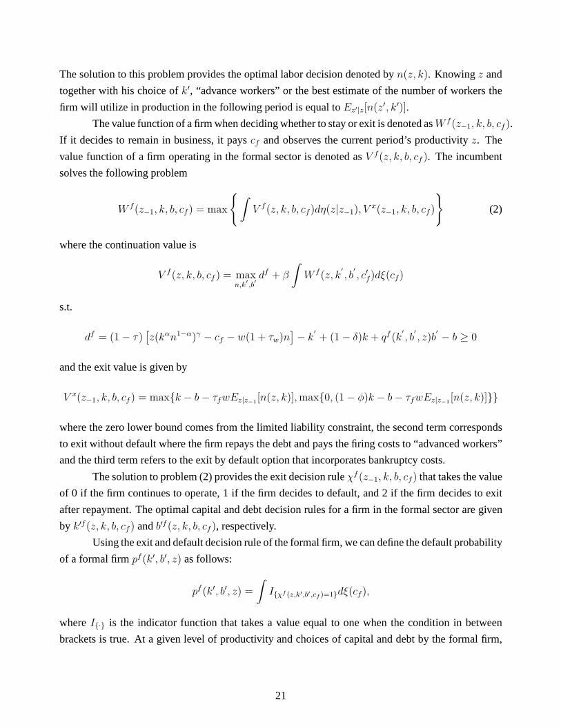
The solution to this problem provides the optimal labor decision denoted byn(z, k). Knowingz and
together with his choice ofk′, “advance workers” or the best estimate of the number of workers the
firm will utilize in production in the following period is equal toEz′|z[n(z′, k′)].
The value function of a firm when deciding whether to stay or exit is denoted asW f(z−1, k, b, cf).
If it decides to remain in business, it payscf and observes the current period’s productivityz. The
value function of a firm operating in the formal sector is denoted asV f(z, k, b, cf ). The incumbent
solves the following problem
W f(z−1, k, b, cf) = max
∫V f(z, k, b, cf )dη(z|z−1), V
x(z−1, k, b, cf)
(2)
where the continuation value is
V f(z, k, b, cf ) = maxn,k
′,b
′
df + β
∫W f(z, k
′
, b′
, c′f)dξ(cf)
s.t.
df = (1− τ)[z(kαn1−α)γ − cf − w(1 + τw)n
]− k
′
+ (1− δ)k + qf (k′
, b′
, z)b′
− b ≥ 0
and the exit value is given by
V x(z−1, k, b, cf) = maxk − b− τfwEz|z−1[n(z, k)],max0, (1− φ)k − b− τfwEz|z−1
[n(z, k)]
where the zero lower bound comes from the limited liability constraint, the second term corresponds
to exit without default where the firm repays the debt and paysthe firing costs to “advanced workers”
and the third term refers to the exit by default option that incorporates bankruptcy costs.
The solution to problem (2) provides the exit decision ruleχf (z−1, k, b, cf) that takes the value
of 0 if the firm continues to operate, 1 if the firm decides to default, and 2 if the firm decides to exit
after repayment. The optimal capital and debt decision rules for a firm in the formal sector are given
by k′f(z, k, b, cf ) andb′f (z, k, b, cf ), respectively.
Using the exit and default decision rule of the formal firm, wecan define the default probability
of a formal firmpf(k′, b′, z) as follows:
pf(k′, b′, z) =
∫Iχf (z,k′,b′,cf )=1dξ(cf),
whereI· is the indicator function that takes a value equal to one whenthe condition in between
brackets is true. At a given level of productivity and choices of capital and debt by the formal firm,
21

the default probability integrates over different values of the fixed costcf to capture those states in
which the firm finds it optimal to exit by default.
4.3 Informal Sector Incumbent
An incumbent firm in the informal sector, after observing fixed operating costcf , can choose to stay
active or to exit the market after a default. More specifically, the informal incumbent firm solves the
following Bellman equation:
W i(k, b, cf ) = maxV i(k, b, cf), k
(3)
where the value of remaining in the informal sector is given by
V i(k, b, cf) = maxn,k
′,b
′
di + β
∫W i(k
′
, b′
, c′f)dξ(cf)
s.t.
di = µl(kαn1−α)γ − cf − wn− k
′
+ (1− δ)k + qi(k′
, b′
)b′
− b ≥ 0
The solution to problem (3) provides the exit decision ruleχi(k, b, cf ) that takes the value of 0
if the firm continues to operate in the informal sector and 1 ifthe firm decides to default. The optimal
capital and debt decision rules are given byk′i(k, b, cf) andb′i(k, b, cf).
Similar to the definition of the default probability for a formal firm, we can derive the default
probability of an informal firm using the exit decision rules. Specifically, the default probability of an
informal firmpi(k′, b′) is:
pi(k′, b′) =
∫Iχi(k′,b′,cf )=1dξ(cf).
4.4 Entrants
The value of a potential entrant (net of entry cost)We is given by:
We =
∫max
W i(0, 0, 0),
∫V f(z, 0, 0, 0)η(z|z0)
dν(z0)− ce (4)
whereV f(z, 0, 0, 0) is the value of starting as a formal firm given by
V f(z, 0, 0, 0) = maxk′,b
′
df + β
∫W f(z, k
′
, b′
, c′f)dξ(cf)
s.t.
df = −w(1 + τw)κ− k′
+ qf(k′
, b′
, z)b′
≥ 0
22

Effectively, an entrant has no capital, no debt, and the costof productioncf equals zero. The entrant
chooses between projects and sectors. The sector and project adoption decisions are made after paying
ce and observing the productivity levelz0, which affects the conditional distribution from which the
first productivity parameter will be drawn. Differences in the volatility of the processes together with
differences in initial productivity are going to generate variation in the decisions made by entrants and
by potential lenders. That introduces differences in behavior as a function of volatility and contract
enforceability. In equilibrium, under free entry,We = 0 will hold. The solution to problem (4)
provides the entry decision ruleΞe(z0) that takes value 0 if the firm decides to enter informal and 1
if the firm decides to enter formal. This will determine the entry productivity threshold to the formal
sectorz∗0 . More specifically, letz∗0 be the value of initial productivity in thehighprocess such that
W i(0, 0, 0) =
∫V f(z, 0, 0, 0)η(z|z∗0).
Then, since it is possible to show that the value of being in the formal sector is increasing in the level
of productivity, the entry decision rule will beΞe(z0) = 1 for z0 ≥ z∗0 and equal to zero otherwise.
The solution to this problem also provides capital and debt decision rulesk′(z, 0, 0, 0) andb′(z, 0, 0, 0)
for a firm that starts operating in the formal sector.
4.5 Lenders
Lenders make loans to formal and informal firms while taking prices as given. Profit for a loanb′ to a
firm in the formal sector with future capitalk′ and, productivityz is
πf(k′
, b′
, z) = −qf(k′
, b′
, z)b′
+1− pf(k
′
, b′
, z)
1 + rb′
+pf(k
′
, b′
, z)
1 + rmin
b′, (1− φ)k′ − τfwEz|z−1
[n(z, k)]− ζb′,
wherepf (k′
, b′
, z) denotes the default probability of this borrower defined before.
Profit for a loanb′ to a firm in the informal sector with future capitalk′ is
πi(k′
, b′
) = −qi(k′
, b′
)b′
+
[1− pi(k
′
, b′
)]
1 + rb′ − ζb′
wherepi(k′
, b′
) denotes the default probability of the informal borrower defined before. In equilib-
rium, the schedule of prices will adjust so thatπf(k′
, b′
, z) = 0 andπi(k′
, b′
) = 0 for all (j, k′, b′, z),
that is, the equilibrium price schedule is given by
qf(k′, b′, z) =1− pf (k′, b′, z)
1 + r+
pf(k′
, b′
, z)
1 + r
minb′, (1− φ)k′ − τfwEz|z−1
[n(z, k)]
b′− ζ, (5)
23

and
qi(k′
, b′
) =
[1− pi(k
′
, b′
)]
1 + r− ζ.
4.6 Definition of Equilibrium
A stationary competitive equilibrium is a set of value functionsW f ,W i, V f , V i, V f, decision rules
(capital, debt, default, exit and sector), a wage ratew, schedule of lending pricesqf(k′, b′, z) and
qi(k′, b′), aggregate distributionsϑ(k, b, z;M) and ϑ(k, b,M) of firms in the formal and informal
sectors, and a mass of entrantsM such that:
1. Given prices, firms’ value functions and their decision rules are consistent with problems (2),
(3) and (4);
2. The free entry condition is satisfied (i.e.,We = 0);
3. Lenders make zero profit for every loan type;
4. The distributions of firmsϑ andϑ are stationary;
5. Aggregate consumption satisfies equation (1);
6. The labor market clears (i.e.,1 =∫nf(z, k)dϑ(k, b, z;M) +
∫ni(k)dϑ(k, b;M)).
5 Calibration
This section calibrates the initial steady state of the model. We start with the parametrization of the
stochastic process in the model to then explain the calibration procedure. The process for productivity
will be discretized to obtain the grid forz and the transition probabilitiesη(z′|z) following the method
explained in Tauchen (1986).30 From the transition matrixη(z′|z), the unconditional probabilityη∗(z)
is derived. The distribution of initial shocks is set toν(z0) = η∗(z). Operating fixed costs are assumed
to take values of0, cf ,∞ and the pdf distribution is denoted byξ(0), ξ(cf), ξ(∞).
To calibrate the model we proceed in two steps. A first set of parameters can be calibrated
without the need to solve the model. In a second step, and taking all other parameters as given, a set of
parameters is chosen in order to match relevant moments fromthe Brazilian economy in 2003.31 The
first set contains the following parametersβ, α, γ, δ, r, ζ, ρ, τ, κ, φ, τw, τf. The second set includes
the next six parametersµh, σh, µl, cf , ξ(0), ξ(cf).
We assume that the discount factorβ = 11+r
. We setr to 8.2 percent, the value observed for
real money market rate in Brazil in 2003. The intermediationcostζ is set to 5.58 percent to match
the overhead cost over assets in year 2003. The capital shareα is set to 1/3, a standard value, and the
parameter that controls the degree of decreasing returnsγ is set to0.85, a value based on previous
30 The number of grid points forz is set to 21.31 We select this year because it correspond to the last period before the reduction in credit costs started and also becauseit is the first year for which we have firm-level data.
24

estimates of the degree of decreasing returns to scale at thefirm level. In particular,γ = 0.85 as in
Restuccia and Rogerson (2008). The depreciation rateδ is set to 7 percent, also a standard value.
The tax structure and the cost of formalization parametersτ, τw, τf , φ, κ are computed di-
rectly from the values reported in theDoing Businessdatabase for the Brazilian economy following
the procedure explained in D’Erasmo and Moscoso Boedo (2012).32 They are set as follows: the tax
rateτ = 0.224, andτw = 0.517; the firing costτf = 0.8846; the bankruptcy costφ = 0.09; and the
entry costκ = 0.739.
The autocorrelation of thehigh-productivity processρ is set to 0.78 as estimated by Ulyssea
(2012) using theRelacao Anual de Informacoes Sociais(RAIS), an annual matched employer-employee
data set collected by the Brazilian Ministry of Labor.33 This dataset captures the universe of formal
firms in Brazil. This is the same dataset we use to compute the moments of the firm-size distribution.
The parameter is in the range of commonly estimated values inthe literature.
Six parameters are left for the second step of the calibration process: the mean of the produc-
tivity process of thehighandlow projectsµh andµl respectively, the volatility of thehighproductivity
processσh, the operating costcf and the associated probabilitiesξ(0), ξ(cf). To obtain values for
these parameters, the following seven moments of the Brazilian economy are targeted:(i) the size
of the formal labor force (46.16 percent), measured as thoseworkers covered by a pension scheme
as reported by Brazilian National Institute of Geography and Statistics (see Figure 6 in the data sec-
tion); (ii) the average size of formal establishments in Brazil (10.8 workers) using data from RAIS
(see Table 3);(iii) the average level of corporate credit to GDP computed using values reported in
Catao, Pages and Rosales (2009), equal to 15.19 percent, as shown in Figure 5;(iv) the average exit
rate of formal firms (equal to 12.9 percent) computed by Ulyssea (2010) using data from RAIS ;(v)
the average exit rate for “large” formal firms (i.e., formal firms with more than 20 workers), which
equals 5 percent, as presented in Bartelsman, Haltiwanger and Scarpetta (2009);(vi) the average age
of informal firms, which equals 8.84 years using data from ECINF reported in (Ulyssea, 2010).34
Identification of the model parameters is key to performing asensitive quantitative exercise.
In what follows, we explain our identification strategy. Since all the moments generated by the model
are a function of all “deep” parameters, it is not possible toassociate individual parameters with indi-
vidual statistics. However, the numerical results suggestthat particular moments are more informative
for identifying particular parameters or set of parameters. First, the size of the informal sector is in-
formative aboutµl since, everything else equal, this parameter determines the entry threshold to the
formal sector and the size of the informal firm. Second, the average size of the formal firm is infor-
32 We use data from the earliest year available (in most cases 2007). We note that, as one would expect from parametersthat reflect institutions at the country level, there is almost no variation over time, so this does not generate an inconsistencywith a calibration based on year 2003.33 Ulyssea (2012) estimated several values that range between0.72 and 0.90, and we choose a value in the middle of thisrange.34 The full description of the moments and the sources can be found in the Data Appendix.
25

mative aboutµh since this parameter determines the average productivity for an incumbent formal
firm. Third, the average corporate credit to GDP is informative ofσh. If productivity is constant and
no other shocks are present, firms have an incentive to borrowonly until they reach their optimal size.
As the volatility of productivity changes, firms’ demand forcredit is also affected. The demand for
credit is a function of the price schedule firms face, and the dispersion of interest rates (a function
of the dispersion of default probabilities) is tightly linked with the dispersion of firm productivity.
Fourth, the average exit rate is informative ofcf since a non-trivial share of firms exit when receiving
this shock, and that share is affected by changes incf . Fifth, the average age of informal firms is
informative ofξ(0) since, in most cases, informal firms survive whencf = 0 and the age of the firm
is directly related to the probability of exit. In particular, it is possible to show that the average age
of an informal firm is equal to[1/Pr(survival informal)] = [1/Pr(exit informal)] ≈ [1/(1 − ξ(0))].
Finally, the average exit rate of “large” firms is informative of ξ(cf) since large firms exit only with
probability[1− ξ(cf)− ξ(0)].
The only parameter left to calibrate is the entry costce. Once this parameter is set the equi-
librium of the model can be computed (i.e., we can obtain the equilibrium wagew, the equilibrium
mass of entrantsM and the equilibrium schedule of pricesqf (k′, b′, z) andqi(k′, b′) to clear the labor
market, to satisfy the free entry condition and to satisfy the zero profit condition of financial inter-
mediaries). However, since it is very hard to obtain information to identify the cost of entry, the
calibration strategy follows the seminal work of Hopenhaynand Rogerson (1993). In particular, the
wage rate is normalized to 1 and used to find the value ofce that, in equilibrium, satisfies the free
entry condition with equality. Note that this also implies deriving endogenously the equilibrium mass
of entrantsM and the menu of pricesqf(k′, b′, z) andqi(k′, b′) that clear the labor market and satisfy
the zero profit condition for financial intermediaries.
Table 4 presents the parameters of the model.35
Table 5 presents the targeted moments in the data and the model. Table 5 shows that the model
approximates the targeted moments relatively well.
After the calibration exercise is done, we test the model in different dimensions. In particular,
we ask how the distribution of operating establishments generated by the model compares with that
of Brazil. We start with the distribution of firms in what is denominated the “micro-sector,” i.e., firms
with up to five employees. Data are from ECINF, which includesthe universe of firms in the “micro-
sector.” Table 6 shows that the model approximates the “Micro-Sector” distribution considerably well.
As in the data, most firms employ no workers or only one worker (80.59 percent in the model vs. 86.6
percent in the data). About 90 percent of firms in the “Micro Sector” in the model are informal
(compared to 87 percent in the data). Since informal firms arevery small, with 0 or 1 workers (both
in the model and in the data), this results in the distribution observed in Table 6.
35 The wage rate and the equilibrium mass of entrants are presented in Table 8 below. The equilibrium menu of prices ispresented in Figure 7.
26
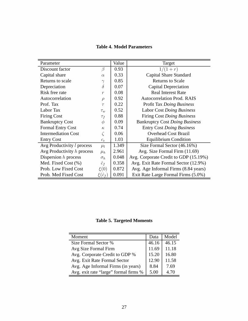
Table 4. Model Parameters
Parameter Value TargetDiscount factor β 0.93 1/(1 + r)Capital share α 0.33 Capital Share StandardReturns to scale γ 0.85 Returns to ScaleDepreciation δ 0.07 Capital DepreciationRisk free rate r 0.08 Real Interest RateAutocorrelation ρ 0.92 Autocorrelation Prod. RAISProf. Tax τ 0.22 Profit TaxDoing BusinessLabor Tax τw 0.52 Labor CostDoing BusinessFiring Cost τf 0.88 Firing CostDoing BusinessBankruptcy Cost φ 0.09 Bankruptcy CostDoing BusinessFormal Entry Cost κ 0.74 Entry CostDoing BusinessIntermediation Cost ζ 0.06 Overhead Cost BrazilEntry Cost ce 1.03 Equilibrium ConditionAvg Productivityl process µl 1.349 Size Formal Sector (46.16%)Avg Productivityh process µh 2.961 Avg. Size Formal Firm (11.69)Dispersionh process σh 0.048 Avg. Corporate Credit to GDP (15.19%)Med. Fixed Cost (%) cf 0.358 Avg. Exit Rate Formal Sector (12.9%)Prob. Low Fixed Cost ξ(0) 0.872 Avg. Age Informal Firms (8.84 years)Prob. Med Fixed Cost ξ(cf) 0.091 Exit Rate Large Formal Firms (5.0%)
Table 5. Targeted Moments
Moment Data ModelSize Formal Sector % 46.16 46.15Avg Size Formal Firm 11.69 11.18Avg. Corporate Credit to GDP % 15.20 16.80Avg. Exit Rate Formal Sector 12.90 11.58Avg. Age Informal Firms (in years) 8.84 7.69Avg. exit rate “large” formal firms % 5.00 4.70
27

Table 6. “Micro-Sector” Firm Size Distribution
Data % Model %# of Workers Frac. Firms CDF Frac. Firms CDF0 86.6 86.60 80.59 80.591 7.4 94.00 18.39 98.982−3 4.6 98.60 0.22 99.214−5 1.40 100.00 0.80 100.00
Note: “Micro-Sector” corresponds to firms with 5 or less employees. Source is ECINF survey, arepresentative cross-section of small firms (5 or less employees) collected at the national level.
We can now look at the distribution across the formal and informal sectors. Using data from
RAIS and ECINF, Table 7 presents the distribution of firms conditional on whether firms operate in
the formal or the informal sector.
The model does a good job of generating the right distributions of operating establishments in
the formal and informal sector, with some caveats. In the formal sector, it generates the right number
of establishments with less than nine employees, but missesat the very low end of the distribution
(less than five employees) and at the very top (firms with more than 99 workers).36 Table 7 shows that
the model is right on target for the distribution of informalestablishments.
As additional tests of the model, we show in Table 8 below thatthe model also captures the
first and second moments of the distribution of corporate spreads. The average corporate spread in
the model is 12.48 percent, versus 14.37 percent in the data.The cross-sectional standard deviation
of corporate spreads in the model is 5.08 percent, compared to 7.96 percent in the data.
6 Experiment: Reducing the Cost of Credit
The objective of this paper is to analyze the effects of the reduction in credit costs on the size of the
firm, the amount of credit in the economy and the level of formality. The experiment can be interpreted
as a counterfactual experiment where we measure the effectsof reducingr and ζ to the observed
values in 2010 and measure the steady state to steady state effect. A summary of our experiment
can be described as follows. First, we calibrated the model to the Brazil economy. In this case,
we normalizew = 1 to then iterate on the set of loan pricesqfj (k′
, b′
, z) andqi(k′
, b′
) until lenders
36 A different entry process into the formal sector can correctthis problem. One alternative is to assume that firms receivea signal of their initial productivity before entering, as opposed to an initial draw from the productivity distribution. If thecorrelation of the signal and the initial productivity is lower than that used for the productivity process, firms that originallyinvested a large amount of capital can find themselves with low productivity and hiring a small amount of workers in theinitial period. Another alternative is to assume that the demand for new firms depends on the time the firm has spent inthe market. A final option is to incorporate a detection probability when firms are in the informal sector. When detectedfirms are forced to formalize, that would move a set of small firms to the formal sector, generating an increase in the 1-4bin. The analysis of these alternatives is beyond the scope of this paper.
28

Table 7. Firm Size Distribution
Formal Size Distribution Data % Model %# of Workers Frac. Firms CDF Frac. Firms CDF0-4 69.58 69.58 24.85 24.854−9 15.22 84.80 39.99 64.849 −19 8.06 92.86 32.09 96.9319−49 4.43 97.29 3.06 99.9949−99 1.36 98.64 0.01 100.0099−249 0.82 99.46 0.00 100.00>249 0.54 100.00 0.00 100.00
Informal Size Distribution Data % Model %# of Workers Frac. Firms CDF Frac. Firms CDF0 80.12 80.12 81.34 81.341 12.23 92.35 18.66 100.002−3 5.88 98.23 0.00 100.004−5 1.77 100.00 0.00 100.00
Note: Source of Formal Size Distribution is RAIS that collects information on all formally-registeredı¬rms. Source for Informal Size Distribution is ECINF survey arepresentative cross-section of small
firms (5 or less employees) collected at the national level.
make zero profit on each contract and to find the mass of potential entrantsM that clears the labor
market and the value of entry costce that satisfies the zero entry condition. Next, we adjust the credit
market condition parametersr, ζ to the values observed in 2010 (r = 4.7 percent andζ = 3.31
percent, respectively), and iterate on the wage ratew and loan pricesqf(k′
, b′
, z) andqi(k′
, b′
) until
lenders make zero profits and the zero entry condition is satisfied (givence obtained in the benchmark
economy). Finally, the mass of entrantsM adjusts to clear the labor market. We start by presenting
results on the most relevant aggregates to then explain the effects on the firm size distribution.
Table 8 presents how the main aggregates are changed from thebenchmark to the equilibrium
with lower costs of credit. As in the data, after a reduction in credit costs (i.e.↓ r, ↓ ζ), the model
generates a rise in corporate credit to GDP and the size of theformal sector. Both the increase in
credit to GDP and the size of the formal sector are larger thanin the data. In particular, the increase
in credit in the model is around 87.89 percent, whereas in thedata it is 57.21 percent. Moreover, the
increase in the formal labor force is 45.07 percent in the model, versus 19.95 percent observed in the
data. One possible explanation for the overshoot is the factthat we are comparing steady state with
steady state, whereas in the data firms might not expect the reduction in the cost of credit (and the
implied size of credit to GDP and formal sector) to be permanent at the level observed in 2010.
29

Table 8. Aggregate Results Reducing the Cost of Credit
Data % Model %2003 2010 ∆ Benchmark ↓ r, ↓ ζ ∆
Corp. Credit to Output 15.19 23.88 57.21 16.80 31.57 87.89Formal Labor Force 46.16 55.37 19.95 46.15 66.95 45.07TFP - - - 1.62 1.86 15.40Output Per Worker 13.85 15.97 15.31 2.31 2.81 21.64Capital Per Worker 36.37 37.85 4.07 2.95 3.46 17.32Avg Spread (%) 14.37 12.93 -10.02 12.48 9.74 -21.96Std. Dev Spread (%) 7.96 9.92 24.62 5.08 5.69 12.01Avg Size Formal Firm 11.69 12.95 10.76 11.18 10.18 -8.94Mass Entrants - - - 0.12 0.10 -22.03Wage ratew - - - 1.00 1.12 12.03Entry/Exit Rate Formal 12.9 - - 11.58 13.89 19.95
Note: Output per worker and Capital per worker in the data computed from Penn World Table.Values in1, 000′s. In the case of these variables, only the change is comparable with the model
counterpart due to the model normalization.
Table 8 also shows that the reduction in credit costs has important aggregate productivity
effects. In order to compute total factor productivity in the model and the data, we follow the cross-
country studies such as Klenow and Rodrıguez-Clare (1997)or Hall and Jones (1999). They compute
the following equation.
TFP =Y
KαH(1−α),
whereY denotes aggregate output,K denotes aggregate capital,H denotes some aggregate for labor
(usually adjusted for human capital) andα is the capital share. We do exactly the same in the model,
where aggregate output is the sum across both formal and informal establishments, aggregate capital
is the sum of capital across establishments in both sectors and our aggregate measure of labor equals
one. Aggregate productivity (TFP ) in the model increases more than 15 percent. The increase in
productivity generates an increase in output per worker of about 21.64 percent, and an increase of
17.32 percent is observed in capital per worker.
Once the costs of credit are reduced, the value of creating a firm increases, generating an in-
crease in the entry rate (+ 19.95 percent). This results in anincrease in the wage rate (12.03 percent).
This is necessary to clear the labor market, since at the original wage rate aggregate demand for labor
exceeds aggregate supply. The increase in wages, together with the reduction in credit costs, induces
firms to substitute away from workers into capital. This results in the observed reduction in the av-
erage size of the formal firm in Brazil as opposed to the increase observed in the data. We note here
that the experiment provides a counterfactual where the cost of credit is reduced using the benchmark
30

economy as starting point. In the data, other factors such aschanges in trade costs and labor regula-
tions (not studied in this paper) affected the size of the formal firm in Brazil. Moreover, there was a
change in the way that RAIS data (our data for formal firms) were collected when comparing the year
2003 to 2010. More specifically, by the year 2006, reference companies and other organizations were
classified according to version 1.0 of the NCEA (National Classification of Economic Activities). In
2007, with the objective of maintaining international comparability, and to equip the country with a
classification of economic activities updated with the changes in the production system of the com-
pany, version 2.0 of the NCEA (National Classification of Economic Activities) went into effect. The
methodology for identification of active units has also beencompletely redesigned from the reference
year 2007 onwards. Unlike previous years, the new selectioncriteria take into consideration not only
completing the declaration of RAIS and research base year, but also a range of other indicators of
economic activity of the unit.
6.1 Firm-Level Effects
Changes in the cost for financial intermediaries have a first order effect on the prices that firms pay for
borrowing. This translates into lower default probabilities that in turn reduce bond prices even further.
This affects the firm size distribution mainly by three channels: first, it induces incumbent firms to
hold a different composition of debt and capital. Second, itaffects the entry and exit thresholds. By
reducing the entry threshold (since the value of the firm is higher) it reduces the average productivity
level of the entrant firm. However, higher entry also resultsin a higher level of competition and higher
wages that translate into more exit. The latter effect also impacts the share of firms producing in the
informal sector (those with lower productivity). This has an extra effect on labor demand and the level
of efficiency in the economy. We start by describing the effect on prices to then present the effects on
the distribution of debt, capital and labor. We then show howthe entry threshold is affected to finally
present the productivity composition in each economy.
Figure 7 presents the schedule of prices in the benchmark case (denoted byq0) and the econ-
omy with lower r and ζ (denoted byq1) as a function ofb′ for different levels of capitalk′ ∈
kL, kM , kH (i.e.,k′ taking a low, medium and high value from the equilibrium distribution). Bond
prices are decreasing in debt levels and capital, since the default probability and the expected recovery
for lenders is decreasing in debt and capital. The higher default probability is translated into higher
interest rates. Importantly, this figure shows that bond prices are lower (i.e., interest rates are higher)
in the benchmark economy than in the case with lowerr andζ for every combination of capital and
debt levels. This effect allows firms to borrow more (as we will show below) in the case with lowerr
andζ . As firms increase their borrowing level bond prices increase. However, as was noted in Table
8, the average spread decreases by 21.96 percent, so the effect of higher bond prices (everything else
equal) dominates.
31

Figure 7. Bond Prices Formal Firm: Benchmark vs↓ r, ζ
0 2 4 6 8 10 12 14 16 18 200
0.1
0.2
0.3
0.4
0.5
0.6
0.7
0.8
0.9
Future debt (b′)
q0(k′
L)
q1(k′L)
q0(k′M
)
q1(k′M
)
q0(k′H
)
q1(k′H
)
As Table 8 showed, whenr andζ are reduced there is an increase in the aggregate credit to
output ratio of 87.89 percent. When bond prices are higher, the value of capital as a buffer stock
against negative productivity shock is reduced (i.e., a lower precautionary motive). That is, firms can
sustain lower levels of capital since it is cheaper to attainthe optimal level of investment by borrowing
in financial markets (this is also reflected in the lower average size of the formal firm). Figure 8 shows
the distribution of the debt to capital ratio in both economies. This figure shows that debt to capital
ratios are considerably lower in the benchmark economy. Themedian firm in the benchmark case has
a debt to output ratio around 0 percent. On the other hand, themedian firm in the economy with lower
r, ζ sustains a debt to output ratio that is close to 35 percent.
Changes in portfolio composition also have important effects on the size of the firm (in terms
of workers). Figure 9 shows the distribution of capital and labor in both economies. The shift in
the distribution of capital (displayed in Panel(i)) together with the increase in wages (+12 percent)
translates into reduction in labor demand for each firm (Panel (ii)). The median firm in the formal
sector in the benchmark economy holds approximately 27 units of capital and hires nine workers in
the benchmark case. The median firm in the counterfactual economy holds approximately 19 units of
capital (a 29 percentreduction) and hires about six workers(a 30 percent reduction).
To take a closer look at the “Micro-Sector” (firms with 5 or less workers) that represents the
largest share of firms in the economy, Table 9 displays how thedistribution of firms for these type of
firms is affected. Recall that the “Micro-Sector” includes formal and informal firms. Table 9 shows
that there is an increase in the share of firms in the smallest bin (those with no workers) and also an
32

Figure 8. Dist. b/k Ratio: Benchmark vs↓ r, ζ
0 0.1 0.2 0.3 0.4 0.5 0.6 0.7 0.8 0.9 130
40
50
60
70
80
90
100
Debt to Capital Ratio (b/k)
Fra
ctio
n o
f F
irm
s (%
)
Bench.↓ r,ζ
Figure 9. Dist. of Capital and Labor: Benchmark vs↓ r, ζ
0 10 20 30 40 50 60 70 80 90 1000
20
40
60
80
100Panel (i): Distribution of Capital
Capital (k)
Fra
ctio
n of
Firm
s (%
)
Bench.↓ r,ζ
0 5 10 15 20 25 300
20
40
60
80
100Panel (ii): Distribution of Labor
Labor (n)
Fra
ctio
n of
Firm
s (%
)
Bench.↓ r,ζ
33

Table 9. “Micro-Sector” Size Distribution: Benchmark vs ↓ r, ζ
Benchmark % ↓ r, ↓ ζ %# of Workers Frac. Firms CDF Frac. Firms CDF0 80.53 80.53 92.32 92.321 18.38 98.91 0.04 92.362−3 0.32 99.23 2.66 95.024−5 0.77 100.00 4.98 100.00
Table 10. Firm Size Distribution: Benchmark vs↓ r, ζ
Formal Size Distribution Benchmark % ↓ r, ↓ ζ %# of Workers Frac. Firms CDF Frac. Firms CDF0-4 24.85 24.85 35.67 35.674−9 39.99 64.84 58.61 94.289−19 32.09 96.93 5.53 99.8119−49 3.06 99.99 0.19 100.0049−99 0.01 100.00 0.00 100.00
Informal Size Distribution Benchmark % ↓ r, ↓ ζ %# of Workers Frac. Firms CDF Frac. Firms CDF0 81.34 81.34 100.00 100.001 18.66 100.00 0.00 100.002−3 0.00 100.00 0.00 100.004−5 0.00 100.00 0.00 100.00
important increase in the share of firms with four and five workers. The general equilibrium effect,
which results in a larger wage, induces informal and formal firms to hire fewer workers. The increase
in the smallest bin is mostly due to changes in the labor demand of informal firms. On the other
hand, the change in the largest bin is due to changes in the labor demand of formal firms that were not
included in the “Micro-Sector” before but are after the change in credit conditions.
To understand these results better, we now study the distribution of formal and informal firms
individually. Table 10 presents the distribution of formaland informal firms. Table 10 shows that
labor demand is affected in both the formal sector and the informal sector. In the formal sector, the
share of firms in the0−4 worker and 4−9 worker bins increases by approximately by 50 percent. The
share of firms in other size bins are reduced with the largest reductions in the9−19 and19−49 bins.
The increase in wages and the reduction in bond prices also impact the informal size distribution.
Only very small firms remain active in this sector.
34

Figure 10. Entry Threshold: Benchmark vs↓ r, ζ
2.5 3 3.5 4 4.5
0
0.1
0.2
0.3
0.4
0.5
0.6
0.7
0.8
0.9
1
Productivity (z)
Ent
ry: 0
=Inf
orm
al ,
1=F
orm
al,
Bench.↓ r,ζ
6.1.1 Firm-Level Productivity
Changes in the cost of credit impact the firm size distribution via changes in both the entrant’s and
incumbent’s level of productivity. Figure 10 presents the entry threshold to the formal sector (i.e.,
the value ofz∗0 in each case as defined in the solution to the entrant’s problem). Two factors affect
the entry threshold in opposite directions. An increase in the wage rate reduces firm profitability
increasing the threshold. The reduction in loan prices increases the value of the firm and the entry
threshold moves down. As shown in Figure 10, the last factor dominates and results in an entry
threshold to the formal sector that is 5.82 percent lower. This smaller entry threshold results in higher
entry rates. The higher level of entry also results in higherexit rates, increasing the productivity level
of incumbent firms (the “cleansing effect”). The effect of lower productivity of entrants is dominated
by the “cleansing” effect, resulting in a shift to the right of the distribution of firm productivity. Figure
11 shows precisely the distribution of firm-level productivity in the formal sector in both economies.
It is evident from Figure 11 that productivity in the formal sector increases after the reduction in credit
costs. To understand the total effect on aggregate productivity (TFP) of reducing the cost of credit, we
need to understand how production is allocated across firms of different productivity and incorporate
the informal sector into the analysis. Figure 12 presents the distribution of aggregate production (for
the entire economy) as a function of firm-level productivity.
Figure 12 shows that production is allocated more efficiently when credit costs are lower. The
distribution of production shifts to the right when comparing the benchmark case versus the economy
with lower r, ζ. An important factor generating this result is the share of firms operating in the
35

Figure 11. Productivity Distribution Formal Sector: Benchmark vs ↓ r, ζ
2 2.5 3 3.5 4 4.5 50
2
4
6
8
10
12
14
16
18
Firm Productivity (z)
Fra
ctio
n of
Firm
s (%
)
Bench.↓ r,ζ
Figure 12. Distribution of Production (both sectors): Benchmark vs ↓ r, ζ
1.5 2 2.5 3 3.5 4 4.510
20
30
40
50
60
70
80
90
100
Firm Productivity (z)
Fra
ctio
n of
Agg
rega
te P
rodu
ctio
n (%
)
Bench.↓ r,ζ
36

Table 11. Firm Productivity Decomposition
Group z Ω z cov(zs, ωfs )
Benchmark 2.407 0.373 3.0908 0.035↓ r, ζ 2.771 0.213 3.0904 0.067
informal sector. The share of formal firms increases in the counterfactual economy by almost 37
percent. The reduction in productivity in the formal sectordue to the lower entry threshold is more
than compensated by this effect, increasing aggregate TFP.
To explore this effect even further we use a decomposition ofweighted average plant-level
productivity originally proposed by Olley and Pakes (1996), which has also been by, for example,
Bartelsman, Haltiwanger and Scarpetta (2008):
z =
∫zsωsds = Ωµl + (1− Ω)[z + cov(zs, ω
fs )]
wherez is the average of plant level productivity weighted by output share,Ω is the informal share of
output,ωs are the output shares of each establishment,ωfs are the output shares of each establishment
in the formal sector, andz is the un-weighted mean productivity in the formal sector. Therefore, out-
put weighted productivity can be decomposed into three terms. First is the effect of informal activity
given byΩ, and then the formal weighted productivity, which can be decomposed into the unweighted
average of firm-level productivity plus a covariance between output share and productivity. The co-
variance captures allocative efficiency within the formal sector because it reflects the extent to which
firms with higher-than-average productivity have a greatermarket share. Table 11 displays the values
of this decomposition for both economies.
We observe that the value of output-weighted productivity correlates with our value of ag-
gregate TFP. As the cost of credit decreases, the value ofz increases (+15 percent). This effect is
generated by an important shift into the formal sector (the share of informal output decreases by 42
percent) and by a better allocation of resources in the formal sector (evidenced by the 91 percent
increase in thecov(zs, ωfs ) term).
6.2 Decomposing the Effect ofr and ζ
Our main quantitative experiment consisted of analyzing the effects of a joint reduction inr andζ . If
one takes Brazil as a small open economy, one can think of changes inr to be outside the set of factors
the government can control and changes inζ as being a function of government policies. For this
reason, it is important to understand the source of the aggregate effects. We perform a counterfactual
experiment where we change one parameter at a time and compare it to the final joint result. Table
37

Table 12. Decomposing the effects ofr and ζ
only ↓ ζ only ↓ r ↓ r, ↓ ζCorp. Credit to Output 1.98 1.31 1.88Formal Labor Force 0.90 0.91 1.45Output Per Worker 1.03 1.02 1.22
1.03 1.02 1.17TFP 1.02 1.01 1.15Avg Spread (%) 1.13 0.67 0.78
1.25 1.26 1.12Avg Size Formal Firm 1.12 1.15 0.91
1.17 1.12 0.78Wage ratew 1.04 1.03 1.12Entry/Exit Rate Formal 1.02 1.00 1.2
Note: Values are relative to benchmark case.
12 presents the results of these experiments. All values arereported as a share of the values in the
benchmark economy.
Table 12 shows that most of the effect on the level of credit iscoming from a reduction in
ζ (the proportional cost of generating a loan). Reductions inthe risk-free interest rater generate an
increase in credit that is only 1/3 of the overall effect.37 The intuition can be found in equations (5)
and (??). A change inζ has a first order effect on pricesqf andqi, while changes inr affect prices
qf andqi weighted by the corresponding default probability. This isreflected in the observed average
spread. The model generates a higher spread consistent withhigher borrowing when onlyζ changes,
as opposed to a lower spread whenr is lower.
Interestingly, we observe in Table 12 that there is an interaction effect betweenζ andr that
allows the model to generate the overall change in the size ofthe formal sector. Whenζ and r
change individually there is a reduction in the size of the formal sector. Both a lowerζ and a lower
r are needed to make the model move in the direction observed inthe data. We can understand this
result by noting that informal firms also have access to credit (at pricesqi), and changes inζ andr
also change their menu of prices. When only one of the parameter changes, all firms have access to
better credit terms and demand more workers (reflected in higher wages). The increase in the wage
rate reduces the incentives to enter the formal sector, increasing the entry threshold, and this results
in a smaller formal sector. This is also evident in the largersize of the formal firm whenζ andr
change individually. When bothζ andr change together the effect of better credit terms dominates
37 Recall that the percent change inζ andr are approximately similar (44 percent and 37 percent, respectively), ζ goesfrom 5.58 percent to 3.31 percent andr goes from 7.5 percent to 4.7 percent.
38

the increase in the wage rate and the formal sector increases. Consistent with this, the change in the
entry rate when bothζ andr change is larger than the sum of the individual changes.
7 Conclusion
This paper develops a firm dynamics model with endogenous formal and informal sectors to quanti-
tatively evaluate how much of the change in corporate creditand the size of the formal sector can be
attributed to an increase in the efficiency of the financial sector (measured as a reduction in the cost
of funds for financial intermediaries and an increase in their efficiency in extending loans).
The quantitative exercise shows that, as a response to the changes in the financial sector, the
model generates an increase in credit to GDP of 87.89 percent, paired with an increase in the size of
the formal labor force of 45.07 percent. This is consistent with what was observed in the data for the
same period in Brazil. The increase in the level of formalization and the better allocation of resources
induce an increase in measured aggregate TFP of 15.40 percent and weighted firm-level productivity
of 16 percent. To understand the overall results even further, we analyze the changes in the financial
sector one by one. Interestingly, we find that most of the effect on the level of credit is coming from
the increase in the level of efficiency of extending loans (asopposed to changes in their funding costs).
Moreover, the experiments show that effects in terms of the size of the formal sector are not additive,
since there is an important interaction effect between the level of efficiency and the cost of funds for
intermediaries that allows the model to generate the overall change.
This model shows that changes in the cost of credit are important to generate an increase in
the size of the formal sector, the amount of credit and aggregate productivity. One possible avenue for
future research is the study of the optimal size and timing ofthe structural reforms affecting financial
intermediaries. Moreover, important institutions that affect the cost of formality (such as the cost of
entry and the level of taxes) interact with the cost of creditsince they affect the incentives to enter
and to exit by repayment or default. The extent to which changes in credit conditions are effective
depends on whether these institutions are also reformed or not. The analysis of joint reforms is another
interesting line for future research.
39

8 ReferencesAlfaro, L., A. Charlton and F. Kanczuk, F. 2009. “Plant-SizeDistribution and Cross-Country IncomeDifferences.” In: J. Frankel and C. Pissarides, organizers. NBER International Seminar on Macroeco-nomics 2008. Chicago, United States: University of Chicago Press and National Bureau of EconomicResearch.
Antunes, A., and T. Cavalcanti. 2007. “Start Up Costs, Limited Enforcement, and the HiddenEconomy.”European Economic Review51: 203-224.
Araujo, A.P., R.V.X. Ferreira and B. Funchal. 2012. “The Brazilian Bankruptcy Law Experi-ence.”Journal of Corporate Finance18(4): 994-1004
Arellano, C., Y. Bai and J. Zhang. 2010. “Firm Dynamics and Financial Development.”Minneapolis, United States: University of Minnesota. Manuscript.
Atkeson, A., and P. Kehoe. 2007. “Modeling the Transition toa New Economy: Lessons fromTwo Technological Revolutions.”American Economic Review97(1): 64-88
Barro, R., and J. Lee. 2000.“International Data on Educational Attainment: Updates andImplications.” CID Working Paper 42. Cambridge, United States: Harvard University, Center forInternational Development.
Bartelsman, E., J. Haltiwanger and S. Scarpetta. 2009. “Cross-Country Differences in Produc-tivity: The Role of Allocative Efficiency.” NBER Working Paper 15490. Cambridge, United States:National Bureau of Economic Research.
Beck, T., and A. Demirguc-Kunt. 2009. “Financial Institutions and Markets across Countriesand over Time: Data and Analysis.” Policy Research Working Paper 4943. Washington, DC, UnitedStates: World Bank.
Bertrand, M., and F. Kramarz. 2002. “Does Entry Regulation Hinder Job Creation? EvidenceFrom The French Retail Industry.”Quarterly Journal of Economics117(4): 1369-1413.
Bruhn, M., 2008. “License to Sell: The Effect of Business Registration Reform on En-trepreneurial Activity in Mexico.” Policy Research Working Paper 4538. Washington, DC, UnitedStates: World Bank.
Carvalho and Valli. 2011. “Fiscal Policy in Brazil through the Lens of an Estimated DSGEModel.” Working Paper 240. Brasilia, Brazil: Central Bank of Brazil.
Catao, L., C. Pages and M.F. Rosales. 2009. “Financial Dependence, Formal Credit andInformal Jobs.” Working Paper IDB-WP-118. Washington, DC,United States: Inter-American De-velopment Bank.
Castro, R., G. Clementi, G., MacDonald. 2009. “Legal Institutions, Sectoral Heterogeneity,and Economic Development.”Review of Economic Studies76(2): 529-561.
Cooley, T., and V. Quadrini. 2001. “Financial Markets and Firm Dynamics.”American Eco-nomic Review91(5): 1286-1310.
D’Erasmo, P., and H.J. Moscoso Boedo. 2012. “Financial Structure, Informality, and Devel-opment.”Journal of Monetary Economics59(3): 286-302.
D’Erasmo, P., H.J. Moscoso Boedo and A. 2012a. “Misallocation, Informality, and HumanCapital.” College Park, Maryland, United States: University of Maryland. Mimeographed document.
Djankov, S. et al. 2002. “The Regulation Of Entry.”Quarterly Journal of Economics117(1):1-37.
Djankov, S. et al. 2008. “Debt Enforcement Around the World.” Journal of Political Economy116(6): 1105-1149.
40

Djankov, S. et al. 2010. “The Effect of Corporate Taxes on Investment and Entrepreneurship.”American Economic Journal: Macroeconomics2(3): 31-64.
Duarte M., and D. Restuccia. 2010. “The Role of the Structural Transformation in AggregateProductivity.”Quarterly Journal of Economics125(1): 129-173.
Erosa, A., and A. Hidalgo Cabrillana. 2008. “On Finance as a Theory of TFP, Cross-IndustryProductivity Differences, and Economic Rents.”International Economic Review49(2): 437-473.
Fajnzylber, P., W.F. Maloney and G.V. Montes-Rojas. 2008. “Does Formality Improve Micro-firm Performance? Evidence from the Brazilian SIMPLES Program.” Journal of Development Eco-nomics94: 262-276
Funchal, B., and M. Clovis. 2008. “O Impacto da Nova Lei de Falencia na Estrutura de Capitaldas Empresas Brasileiras.” Anais do XXXVI Encontro Nacional de Economia, ANPEC, AssociacaoNacional dos Centros de Posgraduacao em Economia, Rio deJaneiro, Brazil.
Guner, N., G. Ventura and Y. Xu. 2008. “Macroeconomic Implications of Size-DependentPolicies.”Review of Economic Dynamics11: 721-744.
Hall, R., and C. Jones. 1999. “Why Do Some Countries Produce So Much More Output perWorker Than Others?”Quarterly Journal of Economics114(1): 83-116.
Hopenhayn, H. 1992. “Entry, Exit, and Firm Dynamics in Long Run Equilibrium.” Econo-metrica60(5): 1127-1150.
Hopenhayn, H., and R. Rogerson. 1993. “Job Turnover and Policy Evaluation: A GeneralEquilibrium Analysis.”Journal of Political Economy101: 915-938.
La Porta, R., and A. Shleifer. 2008. “The Unofficial Economy and Economic Development.”Brookings Papers on Economic Activity(Fall): 275-352.
Loayza, N., 1996. “The Economics of the Informal Sector: A Simple Model and Some Em-pirical Evidence from Latin America.”Carnegie-Rochester Conference Series on Public Policy45:129-162
McKenzie, D., and Y. Seynabou Sakho. 2010. “Does It Pay Firmsto Register for Taxes? TheImpact of Formality on Firm Profitability.”Journal of Development Economics91(1): 15-24.
Moscoso Boedo, H., and T. Mukoyama. 2012. “Evaluating the Effects of Entry Regulationsand Firing Costs on International Income Differences.”Journal of Economic Growth, forthcoming.
Olley, S., and A. Pakes. 1996. “The Dynamics of Productivityin the TelecommunicationsEquipment Industry.”Econometrica64(6): 1263-1297.
Perry, G. et al. 2007. “Informality: Exit and Exclusion.” Washington, DC, United States;World Bank.
Pratap, S., and E. Quintin. 2008. “The Informal Sector in Developing Countries: Output,Assets, and Employment.” In: J. Davies, editor.Personal Wealth from a Global Perspective. NewYork, United States: Oxford University Press.
Quintin, E., 2008. “Contract Enforcement and the Size of theInformal Economy.”EconomicTheory37: 395-416.
Rajan, R., and L. Zingales. 1998. “Financial Dependence andGrowth.” American EconomicReview88: 559-586.
Rauch, J., 1991. “Modelling the Informal Sector Formally.”Journal of Development Eco-nomics35(1): 33-47
Restuccia, D., and R. Rogerson. 2008. “Policy Distortions and Aggregate Productivity withHeterogeneous Establishments.”Review of Economic Dynamics1124: 707-720.
41

Schneider, F., and D. Enste. 2000. “Shadow Economies: Size,Causes, and Consequences.”Journal of Economic Literature38: 77-114.
Schneider, F., A. Buehn and C. Montenegro. 2010. “Shadow Economies All over the World:New Estimates for 162 Countries from 1999 to 2007.” Policy Research Working Paper 5356. Wash-ington, DC, United States: World Bank.
Tauchen, G. 1986. “Finite State Markov-Chain Approximation to Univariate and Vector Au-toregressions.”Economics Letters20: 177-81.
Ter Minasian, T. 2012. “Structural Reforms in Brazil: Progress and Unfinished Agenda.” Pol-icy Brief IDB-WP-158 Working Paper. Washington, DC, UnitedStates: Inter-American DevelopmentBank.
Tybout, J. 2000. “Manufacturing Firms in Developing Countries: How Well Do They Do, andWhy?” Journal of Economic Literature38: 11-44.
Ulyssea, G. 2010. “Regulation of Entry, Labor Market Institutions and the Informal Sector.”Journal of Development Economics91: 87-99.
2012. “Formal and Informal Firms’ Dynamics.” Chicago, United States: University ofChicago, Department of Economics. Manuscript.
42

9 Data AppendixThis section provides a description of the variables used inthe paper and their sources. A set of filesthat contains every variable used in the paper and that can bemade public accompanies this appendix.First, an Excel file BrazilIDB all data.xls that contains all the aggregate variables (cost ofcredit, sizeof formal sector, credit data, institutions data, as well asthe distribution of informal firms). Second,a second set of Stata files from RAIS (our sample of formal firms) in the file Brazil RAIS data.zip.Finally, the set of tables from ECINF (our sample of small firms that contains information on formaland informal firms) in the file BrasilECINF tables.zip
The variables and its sources used are the following (a definition accompanies the data objectwhen needed).
1. Net Interest Margin
• Definition: Accounting value of bank’s net interest revenueas a share of its interest-bearing (total earning) assets.
• Source: Beck and Demirguc-Kunt (2009).
• Note: See World Bank’s website for full data set.
2. Real Money Market Interest Rate
• Definition: Interest Rates, Money Market Rate
• Source: International Financial Statistics
• Note: The nominal rate is converted to real using the consumer price index, also from IFS.
3. Bank Overhead Costs
• Definition: Value of a bank’s overhead costs as a share of its total assets.
• Source: Beck and Demirguc-Kunt (2009).
• Note: See World Bank website for full data set.
4. Corporate loan interest rates (median, average, distribution)
• Definition: Koan interest rate. Data spans all nationwide banking lending to individualfirms above a minimum thresh-old of R$5,000. These data contain information on interestrates and respective lending amounts at the firm level.
• Source: Central Bank of Brazil (BACEN).
• Note 1: Micro Data not publicly available. Aggregates included in annex Excel file.
• Note 2: The nominal rate is converted to real using the consumer price index.
5. Total domestic bank credit to GDP
• Definition: Total Domestic Bank Credit
• Source: Catao, Pages and Rosales (2009) using data of Brazilian Planning Ministry Re-search Institute (ipeadata.gov.br)
43

6. Domestic Bank Credit to the corporate sector to GDP
• Definition: Domestic Bank Credit to the corporate sector
• Source: Catao, Pages and Rosales (2009) using data of Brazilian Planning Ministry Re-search Institute (ipeadata.gov.br)
7. Formal Size Distribution
• Source: RAISRelocao Anual de Informacoes Sociais
• Note 1: Compiled by the Brazilian Ministry of Labor, which requires by law that allformally registered firms report information each year on each worker employed by thefirm.
• Note 2: Micro data not available. We use aggregate tables reported in the IBGE websiteand summary statistics reported in cited papers. I provide aset of stata files and do filesderived from aggregate tables that I used to compute the distribution of firms reported inthe paper (see BrazilRAIS data.zip)
• Note 3: Tables of interest (1996-2010) can be found in “Cadastro Central de Empresas”(Central Register of Enterprises, CEMPRE):http://www.sidra.ibge.gov.br/bda/pesquisas/cempre/default.asp
• The Central Register of Enterprises (CEMPRE) is formed by companies and other orga-nizations and their local units formally constituted, registered in the National Register ofLegal Entities. The update occurs annually from the annual economic surveys of IBGE,in the areas of Industry, Trade, Construction and Services,and administrative records.
8. Informal Size Distribution
• Source: ECINF survey (Pesquisa de Economia Informal Urbana)
• Note 1: This data is a representative cross-section of smallfirms collected at the nationallevel by the Brazilian Bureau of Statistics (IBGE) in 2003. ECINF samples householdslocated in urban areas and seeks to identify the self-employed and employers with up tofive employees in at least one work situation.
• The ECINF offers extensive detail on the main firm and the entrepreneur characteristics ofthe micro-enterprises such as sector revenues, profits employment size, capital stock andtime in business.
• Note 2: IBGE does not provide access to the micro data but provides a large set of de-scriptive tables that can be found inhttp://www.ibge.gov.br/home/estatistica/economia/ecinf/2003/default.shtmunder “TabelasCompletas.”
• Note 3: I provide the table with the distribution of informalfirms in the Excel file thataccompanies this appendix, and I also provide a zip file with the full set of tables (seeBrazil ECINF tables.zip).
9. Measured Institutions: Taxes (profit and payroll), entrycost formal sector and firing costs
44

• Entry Cost: The cost of entering the formal sector corresponds to the reported “costs ofregistering a business and of dealing with licenses to operate a physical locale.” It involvesthe cost of starting a Business measured in time and the cost of starting a business as afraction of income per capita.38 The estimate of the entry cost for Brazil is 0.739 of GNIper capita.
• Taxes:The tax rate paid on profits by the firms is taken from “Paying Taxes - Profit tax(%)” and the payroll tax corresponds to “Paying Taxes - Labortax and contributions (%).”Because both tax rates are expressed as a function of profits,they need to be adjusted andthe labor tax rate expressed as a function of payroll. To do that, the standardized balancesheet and income statements was used to construct the exercise, as explained in Table 1 ofDjankov et al. (2010). The estimated values for Brazil are 22.4 percent and 51.65 percent,respectively.
• Firing Costs:The firing costs are obtained using information on the variable “Firing cost(weeks of wages).” A year corresponds to 52 weeks, so the estimated value of firing oneworker equals 88 percent of the worker’s annual wage.
• Bankruptcy costs:The efficiency of the system in the event of default is measured bythe fraction of the asset value of the firm lost during bankruptcy. The cost of the system(φ), reported as a percentage of the estate’s value, includes court fees and the cost ofinsolvency practitioners, such as legal and accounting fees. The estimated value for Brazilis 9 percent.
• Source: Doing Businessdataset, World Bank. The complete data set can be found athttp://www.doingbusiness.org/custom-query
38 Following D’Erasmo and Moscoso Boedo (2012), the time cost is translated to monetary units by assuming that oneworker has to be employed full time in order for the firm to go through the entry process.
45