accepted to ieee transactions on power … · sator (statcom), the series static ... savings stem...

ACCEPTED TO IEEE TRANSACTIONS ON POWER SYSTEMS, JUNE 2016 1

Hybrid Power Flow Controller Steady-stateModeling, Control, and Practical Application

Behnam Tamimi, Student Member, IEEE, Claudio Canizares, Fellow, IEEE, and Claudia Battistelli, Member, IEEE

Abstract—Steady-state models of the Hybrid Power FlowController (HPFC) for power flow and optimal power flow (OPF)studies are presented in this paper, considering the multiplecontrol modes of the device. A strategy for control mode switchingand limit handling in power flow calculations is proposed. TheOPF model of the HPFC represents all the device control andphysical limits as constraints in the mathematical formulation,so that the HPFC can be optimally dispatched as a part ofthe transmission system control assets. The power flow modelis demonstrated and validated through loadability studies ona two-area benchmark test system, where the OPF model isused to determine the optimal ratings of the device based ona cost-benefit analysis. A study is also presented of the HPFCapplication to Ontario-Canada’s grid, to address particularcongestion problems in this network; an HPFC cost analysis isalso shown for this system. The presented studies demonstrate theapplication of the proposed models for planning and operationstudies, illustrating the performance, effectiveness, and feasibilityof the controller to solve congestion issues in a real grid.

Index Terms—Congestion relief, FACTS, HPFC, modeling,OPF, power flow.

I. INTRODUCTION

FLEXIBLE AC Transmission System (FACTS) controllersoffer new opportunities to better control power systems,

as well as enhance power transfer capabilities [1]. SeveralVoltage-Source Converter (VSC) FACTS have been proposedin the literature, particularly the Static Synchronous Compen-sator (STATCOM), the Series Static Synchronous Compen-sator (SSSC), and the Unified Power Flow Controller (UPFC)[2]. Among these controllers, the UPFC is a versatile devicethat can control various system variables independently [3](e.g. bus voltage magnitudes and transmission line active andreactive power flows), and its application to solve congestionproblems in an actual grid is demonstrated in [4]. However,the capital cost of this controller is a major obstacle for thewide application of this technology in power systems. Thus,a cost effective VSC-based FACTS controller is introducedin [5], which yields operating characteristics similar to thoseof the UPFC while requiring a lower capital investment. Thiscontroller may consist of converters as well as passive compo-nents (e.g. capacitor banks), and is referred to as the HybridPower Flow Controller (HPFC). Compared to the UPFC, thesavings stem from a few structural differences between the two

This work has been supported by NSERC and Hydro One Inc. through aCollaborative Research and Development (CRD) grant.

B. Tamimi, C. Canizares are with the Department of Electrical andComputer Engineering, University of Waterloo, Waterloo, ON, Canada (e-mail: [email protected]).

C. Battistelli is currently with the Department of Electrical andElectronic Engineering, Imperial College, London, UK (e-mail:[email protected]).

devices, including the use of half-sized converters and passiveelements for supplying the bulk of the required reactive power,as discussed in [5].

The benefits of an HPFC are defined by its limits andoperating constraints. Therefore, the impact of the controllerlimits on its performance must be considered during planningand operation stages. However, previously published works onthe HPFC do not discuss the device operating limits and theirimplications in congestion studies adequately [5]–[7]. Thus,in [5], the device is introduced, and an interesting geometricalrepresentation of the devices operating region is presented.An Electromagnetic Transients Program (EMTP) model of theHPFC is briefly studied in [6]. The performance of the HPFCwith regard to improving the power transfer capability of asystem is compared with that of the UPFC in [7], based ontime domain simulations.

In the current paper, a novel model of the HPFC appropriatefor congestion studies, which are for the most part based onpower-flow analyses, and its various possible control modesare presented and applied to address congestion issues. Thecontroller is modeled from the system point of view, andthus its terminals are considered in the model, which isconsistent with its operation requirements. The controller’sinternal variables are also properly represented in the proposedmodel, which allows handling the device limits accurately andthus modeling the multiple control modes defined in this paper.The proposed model is integrated into a widely popular powerflow production program using a sequential approach to allowits integration into commercial power system analysis softwarepackages. An HPFC model for OPF applications is alsointroduced, proposing a concise mathematical model of theHPFC for OPF applications that considers the device ratingsand its control variables and limits directly. These proposedmodels are then used to demonstrate their applications inplanning and operation studies, evaluating the performance andthe effectiveness of the device using realistic test systems andpractical assumptions and scenarios.

The rest of the paper is organized as follows: After re-viewing the basics of the HPFC in Section II, its steady-statecircuit model and associated operating modes are introducedin Section III, together with an effective strategy to handlethe operating limits in power flow studies. The device modelfor OPF applications is presented in Section IV. In Section V,the device is applied to address congestion issues in two testsystems, namely, a two-area system and a detailed model ofOntario-Canada’s grid; several studies based on the proposedmodel and realistic scenarios are carried out to evaluate theperformance and show the benefits of the HPFC, demonstrat-ing the feasibility of the device to solve actual congestion


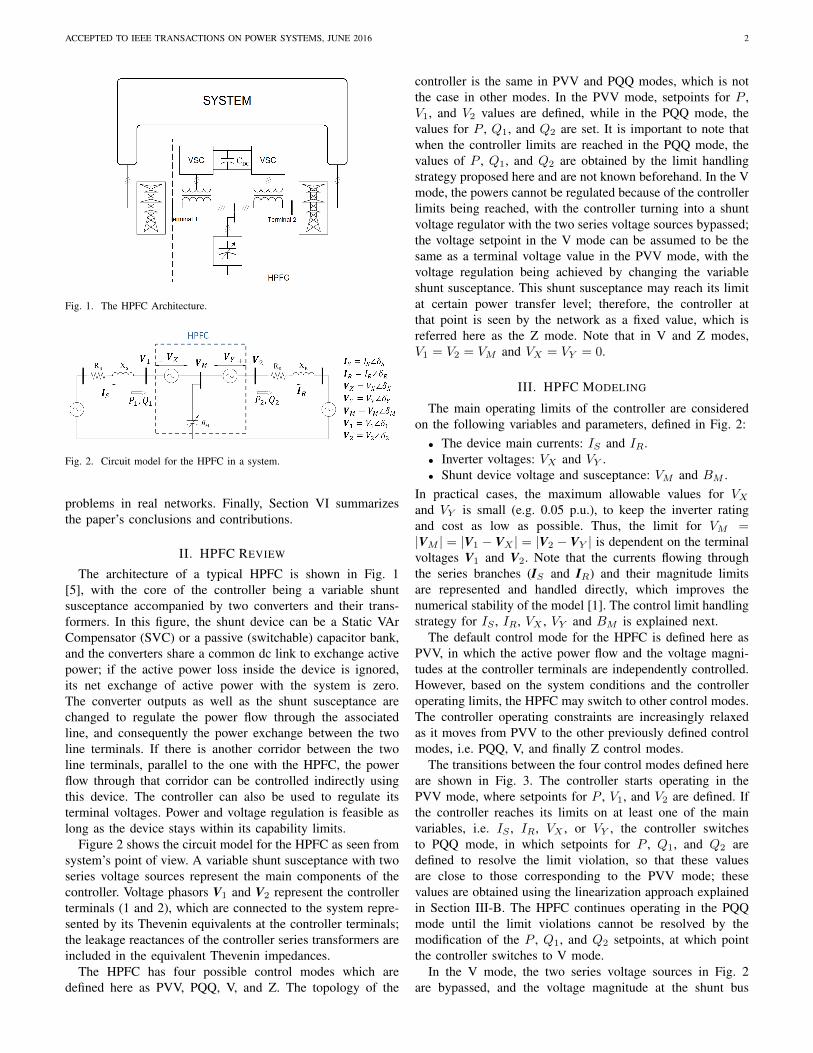
Fig. 1. The HPFC Architecture.

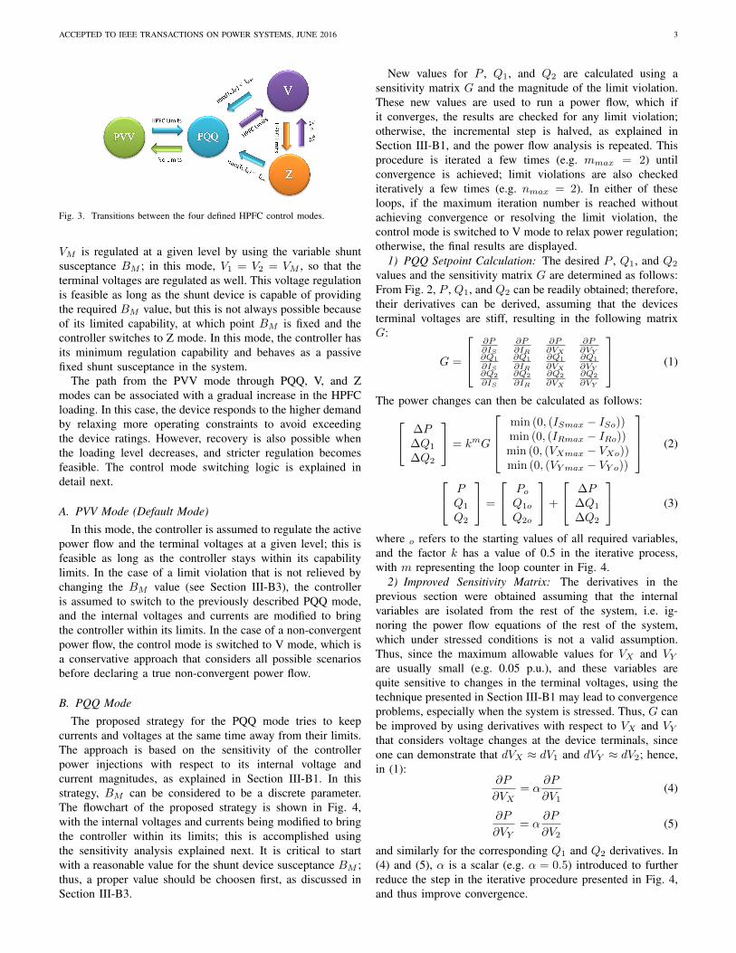
Fig. 2. Circuit model for the HPFC in a system.

problems in real networks. Finally, Section VI summarizesthe paper’s conclusions and contributions.

II. HPFC REVIEW

The architecture of a typical HPFC is shown in Fig. 1[5], with the core of the controller being a variable shuntsusceptance accompanied by two converters and their trans-formers. In this figure, the shunt device can be a Static VArCompensator (SVC) or a passive (switchable) capacitor bank,and the converters share a common dc link to exchange activepower; if the active power loss inside the device is ignored,its net exchange of active power with the system is zero.The converter outputs as well as the shunt susceptance arechanged to regulate the power flow through the associatedline, and consequently the power exchange between the twoline terminals. If there is another corridor between the twoline terminals, parallel to the one with the HPFC, the powerflow through that corridor can be controlled indirectly usingthis device. The controller can also be used to regulate itsterminal voltages. Power and voltage regulation is feasible aslong as the device stays within its capability limits.

Figure 2 shows the circuit model for the HPFC as seen fromsystem’s point of view. A variable shunt susceptance with twoseries voltage sources represent the main components of thecontroller. Voltage phasors V1 and V2 represent the controllerterminals (1 and 2), which are connected to the system repre-sented by its Thevenin equivalents at the controller terminals;the leakage reactances of the controller series transformers areincluded in the equivalent Thevenin impedances.

The HPFC has four possible control modes which aredefined here as PVV, PQQ, V, and Z. The topology of the

controller is the same in PVV and PQQ modes, which is notthe case in other modes. In the PVV mode, setpoints for P ,V1, and V2 values are defined, while in the PQQ mode, thevalues for P , Q1, and Q2 are set. It is important to note thatwhen the controller limits are reached in the PQQ mode, thevalues of P , Q1, and Q2 are obtained by the limit handlingstrategy proposed here and are not known beforehand. In the Vmode, the powers cannot be regulated because of the controllerlimits being reached, with the controller turning into a shuntvoltage regulator with the two series voltage sources bypassed;the voltage setpoint in the V mode can be assumed to be thesame as a terminal voltage value in the PVV mode, with thevoltage regulation being achieved by changing the variableshunt susceptance. This shunt susceptance may reach its limitat certain power transfer level; therefore, the controller atthat point is seen by the network as a fixed value, which isreferred here as the Z mode. Note that in V and Z modes,V1 = V2 = VM and VX = VY = 0.

III. HPFC MODELING

The main operating limits of the controller are consideredon the following variables and parameters, defined in Fig. 2:• The device main currents: IS and IR.• Inverter voltages: VX and VY .• Shunt device voltage and susceptance: VM and BM .

In practical cases, the maximum allowable values for VXand VY is small (e.g. 0.05 p.u.), to keep the inverter ratingand cost as low as possible. Thus, the limit for VM =|VM | = |V1 − VX | = |V2 − VY | is dependent on the terminalvoltages V1 and V2. Note that the currents flowing throughthe series branches (IS and IR) and their magnitude limitsare represented and handled directly, which improves thenumerical stability of the model [1]. The control limit handlingstrategy for IS , IR, VX , VY and BM is explained next.

The default control mode for the HPFC is defined here asPVV, in which the active power flow and the voltage magni-tudes at the controller terminals are independently controlled.However, based on the system conditions and the controlleroperating limits, the HPFC may switch to other control modes.The controller operating constraints are increasingly relaxedas it moves from PVV to the other previously defined controlmodes, i.e. PQQ, V, and finally Z control modes.

The transitions between the four control modes defined hereare shown in Fig. 3. The controller starts operating in thePVV mode, where setpoints for P , V1, and V2 are defined. Ifthe controller reaches its limits on at least one of the mainvariables, i.e. IS , IR, VX , or VY , the controller switchesto PQQ mode, in which setpoints for P , Q1, and Q2 aredefined to resolve the limit violation, so that these valuesare close to those corresponding to the PVV mode; thesevalues are obtained using the linearization approach explainedin Section III-B. The HPFC continues operating in the PQQmode until the limit violations cannot be resolved by themodification of the P , Q1, and Q2 setpoints, at which pointthe controller switches to V mode.

In the V mode, the two series voltage sources in Fig. 2are bypassed, and the voltage magnitude at the shunt bus


Fig. 3. Transitions between the four defined HPFC control modes.

VM is regulated at a given level by using the variable shuntsusceptance BM ; in this mode, V1 = V2 = VM , so that theterminal voltages are regulated as well. This voltage regulationis feasible as long as the shunt device is capable of providingthe required BM value, but this is not always possible becauseof its limited capability, at which point BM is fixed and thecontroller switches to Z mode. In this mode, the controller hasits minimum regulation capability and behaves as a passivefixed shunt susceptance in the system.

The path from the PVV mode through PQQ, V, and Zmodes can be associated with a gradual increase in the HPFCloading. In this case, the device responds to the higher demandby relaxing more operating constraints to avoid exceedingthe device ratings. However, recovery is also possible whenthe loading level decreases, and stricter regulation becomesfeasible. The control mode switching logic is explained indetail next.

A. PVV Mode (Default Mode)

In this mode, the controller is assumed to regulate the activepower flow and the terminal voltages at a given level; this isfeasible as long as the controller stays within its capabilitylimits. In the case of a limit violation that is not relieved bychanging the BM value (see Section III-B3), the controlleris assumed to switch to the previously described PQQ mode,and the internal voltages and currents are modified to bringthe controller within its limits. In the case of a non-convergentpower flow, the control mode is switched to V mode, which isa conservative approach that considers all possible scenariosbefore declaring a true non-convergent power flow.

B. PQQ Mode

The proposed strategy for the PQQ mode tries to keepcurrents and voltages at the same time away from their limits.The approach is based on the sensitivity of the controllerpower injections with respect to its internal voltage andcurrent magnitudes, as explained in Section III-B1. In thisstrategy, BM can be considered to be a discrete parameter.The flowchart of the proposed strategy is shown in Fig. 4,with the internal voltages and currents being modified to bringthe controller within its limits; this is accomplished usingthe sensitivity analysis explained next. It is critical to startwith a reasonable value for the shunt device susceptance BM ;thus, a proper value should be choosen first, as discussed inSection III-B3.

New values for P , Q1, and Q2 are calculated using asensitivity matrix G and the magnitude of the limit violation.These new values are used to run a power flow, which ifit converges, the results are checked for any limit violation;otherwise, the incremental step is halved, as explained inSection III-B1, and the power flow analysis is repeated. Thisprocedure is iterated a few times (e.g. mmax = 2) untilconvergence is achieved; limit violations are also checkediteratively a few times (e.g. nmax = 2). In either of theseloops, if the maximum iteration number is reached withoutachieving convergence or resolving the limit violation, thecontrol mode is switched to V mode to relax power regulation;otherwise, the final results are displayed.

1) PQQ Setpoint Calculation: The desired P , Q1, and Q2

values and the sensitivity matrix G are determined as follows:From Fig. 2, P , Q1, and Q2 can be readily obtained; therefore,their derivatives can be derived, assuming that the devicesterminal voltages are stiff, resulting in the following matrixG:

G =

∂P∂IS

∂P∂IR

∂P∂VX

∂P∂VY

∂Q1

∂IS

∂Q1

∂IR

∂Q1

∂VX

∂Q1

∂VY∂Q2

∂IS

∂Q2

∂IR

∂Q2

∂VX

∂Q2

∂VY

(1)

The power changes can then be calculated as follows: ∆P∆Q1

∆Q2

= kmG

min (0, (ISmax − ISo))min (0, (IRmax − IRo))min (0, (VXmax − VXo))min (0, (VYmax − VY o))

(2)

PQ1

Q2

=

PoQ1o

Q2o

+

∆P∆Q1

∆Q2

(3)

where o refers to the starting values of all required variables,and the factor k has a value of 0.5 in the iterative process,with m representing the loop counter in Fig. 4.

2) Improved Sensitivity Matrix: The derivatives in theprevious section were obtained assuming that the internalvariables are isolated from the rest of the system, i.e. ig-noring the power flow equations of the rest of the system,which under stressed conditions is not a valid assumption.Thus, since the maximum allowable values for VX and VYare usually small (e.g. 0.05 p.u.), and these variables arequite sensitive to changes in the terminal voltages, using thetechnique presented in Section III-B1 may lead to convergenceproblems, especially when the system is stressed. Thus, G canbe improved by using derivatives with respect to VX and VYthat considers voltage changes at the device terminals, sinceone can demonstrate that dVX ≈ dV1 and dVY ≈ dV2; hence,in (1):

∂P

∂VX= α

∂P

∂V1(4)

∂P

∂VY= α

∂P

∂V2(5)

and similarly for the corresponding Q1 and Q2 derivatives. In(4) and (5), α is a scalar (e.g. α = 0.5) introduced to furtherreduce the step in the iterative procedure presented in Fig. 4,and thus improve convergence.


Fig. 4. Control strategy in PQQ mode.

3) Choosing BM : The voltage magnitude on the invertersoutputs depends on the shunt device voltage and thus the valueof BM ; therefore, a “good” BM value facilitates relieving thevoltage limit violations. This is the first step depicted in Fig. 4before the iterative procedure described in Section III-B1. Theprocedure to determine this value is explained next.

Based on the terminals voltages available from a previouspower flow solution, an approximate working guess of VM(and BM ) can be obtained as follows: Figure 5 depicts anexaggerated diagram of the voltage phasors, where the smallestvalues for VX and VY are reached when VM lies between VM1

and VM2. Therefore, to have VM within this interval or closeto it, first VM1 and/or VM2 are obtained using an initial guessfor BM to see if these yield feasible VX and VY ; if not, theinterval between VM1 and VM2 is halved, with the resultingVM yielding new VX and/or VY phasors. If these VX and/orVY are within their magnitude limits, then the associatedvalue of BM is computed; otherwise, the algorithm continuesbisecting the interval until a feasible result, if it exists, isachieved, or a certain maximum iteration number (e.g. 3) isreached. The minimum VX + VY is used to choose whetherto increase or decrease BM , while halving the interval. Thedesired BM value is calculated based on the obtained valuefor VM ; for discrete values of the shunt device, the closest stepto the calculated value is chosen and used in the next step.

C. V ModeIn this mode, the two series voltage sources (see Fig. 2)

are bypassed and V1 = V2 = VM . The voltage magnitude atthe terminals are regulated at a given level using the variableshunt susceptance BM , with no active power flow controlby the device. Thus, the power flow is run assuming the

Fig. 5. Voltage phasor diagram.

device terminals and the shunt bus merged into one bus witha regulated voltage magnitude. If the power flow does notconverge, the control mode switches to Z mode; otherwise,the largest of the input and the output currents (IS and IR)are checked with respect to the inverters’ current limits; if itis within the limits, the device recovers and switches to PQQmode, otherwise, based on the reactive power injection at theshunt bus obtained from the power flow analysis, the requiredBM value is calculated. The shunt device has a maximumlimit; thus, if the calculated BM exceeds its maximum value,the shunt susceptance is fixed at BMmax, and the controlmode is switched to Z mode. Otherwise, the control remainsat V mode and final results are displayed. Note that if BMis discrete, the voltage setpoint in the V mode will varyaccordingly, i.e. is not a fixed value.

D. Z Mode

The Z mode corresponds to the HPFC at its minimumregulating capability. The BM in this case is fixed at its


maximum value and V1 = V2 = VM , and thus the devicebecomes a passive fixed shunt susceptance in the power flowanalysis.

IV. OPF MODEL

The optimal power dispatch for a system can be calculatedusing an OPF formulation; the objective of this optimizationproblem is usually the maximization of social benefit or theminimization of production costs. System operational andsecurity constraints as well as operating limits are usuallyincluded in an OPF formulation. Hence, mathematically theOPF can be stated as follows [8]:

minPG,QG,V,δ

Costs =∑i∈G

Ci (PGi) (6a)

s.t.

PGi − PDi =∑j∈N

ViVj(Gij cos(δi − δj)

+Bij sin(δi − δj)) i ∈ N (6b)

QGi −QDi =∑j∈N

ViVj(Gij sin(δi − δj)

−Bij cos(δi − δj)) i ∈ N (6c)PGimin ≤ PGi ≤ PGimax i ∈ G (6d)QGimin ≤ QGi ≤ QGimax i ∈ G (6e)Vimin ≤ Vi ≤ Vimax i ∈ N (6f)

where Ci (·) stands for the generator i production cost, whichis typically a quadratic function; N and G represent the setof all buses and generators, respectively; PD and QD standfor the active and reactive demand which are assumed fixedhere; PG and QG represent the active and reactive powersof generators; Gij and Bij stand for line parameters; and Vand δ correspond to the bus voltage phasor magnitudes andangles. Other operational or security constraints can be readilyincluded as well (e.g. line flow limits), but were not consideredhere.

A lossless HPFC is considered here as part of the trans-mission system assets for dispatch purposes. In this context,the device can be represented in the OPF using the followingpower and circuit equations associated with Fig. 2:

P1 = Re {V1I∗S} (7)

P2 = Re {V2I∗R} (8)

P1 = P2 (9)

V1 = VX + VM (10)

V2 = VY + VM (11)

VM =

(IS − IRjBM

)(12)

Proper ratings of the device imply a symmetrical loading onthe series inverters, since both are assumed to share the loadequally; this results in the following constraint:

|VX − VY | ≤ ε (13)

where ε is a small tolerance. Furthermore, the ratings ofthe converters and the shunt capacitor impose limits on thevoltage magnitudes VX and/or VY , and current magnitudes ISand/or IR, and BM ; these limits can be modeled through thefollowing constraints:

0 ≤ VX ≤ VXmax (14)

0 ≤ VY ≤ VYmax (15)

0 ≤ IS ≤ ISmax (16)

0 ≤ IR ≤ IRmax (17)

0 ≤ BM ≤ BMmax (18)

Adding the HPFC equations and constraints (7)–(18) to (6)yields the full OPF model of the system including the HPFCfor dispatch purposes. The solution of this optimization prob-lem can be used to determine:• The power dispatch of the system at minimum cost or

maximum social benefit.• The optimal setpoints of the HPFC control variables,

including terminal voltage magnitudes and the devicepower flows.

In other words, the OPF solution yields an optimal powerdispatch and the HPFC optimal control setpoints, correspond-ing to the lowest system operating costs for the assumedconstraints. Also, this formulation, with proper large set ofbounds for the HPFC constraints, can be used to determineoptimal ratings of the device in design and planning studiesfor given system constraints, which is what the OPF model isused for in this paper.

V. RESULTS AND DISCUSSIONS

The results of applying the discussed HPFC models toaddress congestion problems in a two-area benchmark testsystem and in Ontario-Canada’s grid are presented in thissection. In these studies, the power setpoints are varied andthe voltage setpoints are chosen to be the same or very closeto the values corresponding to the base-case conditions. Thisapproach provides a meaningful and yet simple template tostudy and compare the power flow results without and withthe added HPFC. The power flow and OPF studies of the two-area system are performed respectively, using PSAT, which is aMATLAB-based software package for power system analysis[9], and AMPL which is a mathematical modeling tool foroptimization purposes [10]. The power flow and HPFC coststudies of the Ontario system are carried out using PSSrE[11].The detailed power flow model is integrated into thestandard PSSrE solver using a custom Python code, whichwas used to introduce the mathematical model and procedurerequired to represent the HPFC within PSSrE [12].

A. Two-area Test System

A slightly modified version of Kundur’s two-area test sys-tem is used for the analyses presented in this section [13].


Fig. 6. Two-area test system.

TABLE ITIE-LINE PARAMETERS (100 MVA, 230 KV BASE)

From To R [p.u.] X [p.u.] B [p.u.]

7 12 0.00733 0.0733 0.192512 9 0.00733 0.0733 0.096258 9 0.022 0.22 0.19257 13 0.022 0.22 0.09625

1) System Description: The system is loosely based onOntario-Canada’s network, representing the main generators,loads, and east-west system interconnections, which was de-veloped to study small-disturbance oscillations. In this paper,the system is used to analyze congestion management issuesassociated with power flows over the tie-lines between thetwo areas, motivated by the actual congestion studies presentedlater for Ontario-Canada’s grid. Figure 6 shows the single-linediagram of the system, and the original data can be found in[13]. The two areas are connected by a 220-km double-circuittie-line. Both ends of the line are equipped with capacitorbanks. In this study, the tie-line impedances as well as thereactive power demand/support at Buses 7 and 9 are slightlymodified to force the system towards its limits; thus, the tie-line parameters are changed as per Table I, so that the overalltie-line impedance remains basically unchanged. The reactivepower demands at Buses 7 and 9 are 300 MVAr and 50 MVArcapacitive, respectively.

The HPFC is connected between Bus 13 and Bus 8 in thelower corridor. The controller is assumed to start in PVVmode, thus defining setpoints for its active power flow and thevoltage magnitudes at its terminals, which can be set arbitrarilyas desired by the operator or based on a chosen dispatchpolicy. The setpoints are chosen here so that the flows andvoltages are consistent with the base system without HPFCat base load for comparison purposes; however, the setpointscan be chosen optimally for different operating points usingthe proposed OPF model.

2) Power Flow Results: The loadability studies performedon the system assume Buses 9 and 2 as power sink andsource, respectively. Thus, the power transfer between thesetwo nodes is increased until the power flow cannot be solved,gradually increasing the load in 0.1 p.u. steps. The requiredHPFC parameters used here are the following:• Maximum current magnitudes (IS and IR): 2 p.u.• Maximum voltage magnitude for the converters including

transformers (VX and VY ): 0.04 p.u. (9.2 kV).• Discrete shunt susceptance with four equal steps (0.2 p.u.

each): 0 ≤ BM ≤ 0.8 p.u. The size of this capacitorcan be considered reasonable compared to the existing

Fig. 7. PV curves at Bus 9 with and without HPFC.

Fig. 8. HPFC control modes and BM as the loading level increases.

capacitors at Buses 7 and 9.• Active power share of the lower corridor with respect to

the total tie-line flow: 25%.• Voltage magnitude setpoint at the terminals: 0.9557 p.u.The maximum loadability of the system at Bus 9 increases

from 204 MW to 240 MW when introducing the HPFC. Thevoltage profile at the sink-bus Bus 9 is depicted in Fig. 7, withand without the HPFC; observe that the HPFC improves themaximum loadability and voltage profile.

The HPFC control modes and BM values at differentoperating points are shown in Fig. 8. Note that the device startsin the PVV mode and switches to different modes accordingto the system requirements at different operating points as theload increases. At the last four operating points, the HPFChas exhausted its capability limits, and thus behaves as a fixedshunt susceptance in the Z mode. Observe that the algorithmtransitions to the best feasible mode using the available shuntsusceptance steps, based on the procedure depicted in Fig. 4.

3) OPF Results: The optimal voltage ratings of the con-troller can be chosen using the proposed OPF formation


TABLE IIGENERATOR COST C (PG) = a+ bPG + cP 2

G .

Bus No. a [$/h] b [$/MWh] c [$/MW2h] PGmax [MW]

1 800 20 0.002 20002 800 20 0.002 20003 1600 40 0.004 20004 1600 40 0.004 700

Fig. 9. Economic analysis for different voltage ratings: (a) Savings, and (b)Cost-benefit.

assuming the rest of the parameters remain as defined earlier,since current ratings mostly depend on the expected maximumpower flow, and the shunt component is assumed to be known.The generators in the area to the right, i.e. Buses 3 and 4which are closer to the demand centre, are assumed to bemore expensive than the generators in the left area (Buses 1and 2), as illustrated in the generator dispatch cost data inTable II. This uneven pricing allows to study the financialimpact of the tie-line transfer capability, to be relieved by theintroduction of the HPFC. The unit cost of HPFC convertersincluding required installation/constructions is assumed to be$100,000/MVA; this figure for the capacitor banks is close to$20,000/MVAr [14], [15].

The expected annual operation savings due to the deviceinstallation shown in Fig. 9(a) can be calculated using a typicalload duration curve [16]. Note the savings increase as thevoltage ratings increase, as expected. One can compare theeffect of different voltage ratings by subtracting the installationcosts from the savings, resulting in the cost benefit curvedepicted in Fig. 9(b) which has a maximum at a 0.04 p.u.voltage rating.

B. Application to Ontario-Canada’s Grid

A detailed model of the Ontario-Canada system is used hereto examine the use of the HPFC model within a realisticallylarge system, motivated by the interest in and relevance ofthese studies to several entities associated with the provincial

electricity grid. The prospective HPFC installation would pro-vide system operators with the ability to control the flows andadequately regulate the voltage profile in the grid, thus pro-viding congestion relief at peak-demand and voltage supportin the case of contingencies. Therefore, the performance ofthe HPFC under realistic conditions and scenarios are studiedhere, and the results are presented and discussed next.

1) Network Model: The base-case dataset for the gridwas obtained from Ontario-Canada’s Independent ElectricitySystem Operator (IESO), and contains information for a powerflow solution at a peak demand period [17]. It spans the powernetwork from New Brunswick to Kentucky, including Ontario,New York, and areas in between. It has 6895 buses, 38085branches, 1890 generator units, and a total load of 267 GW.

2) Potential HPFC Locations: Based on the input fromthe IESO, the following four locations on the Ontario gridwere studied for the potential HPFC installation, given thatthe associated lines are prone to congestion problems, asdetermined based on PV-curves and related studies performedfor different loading scenarios:

a) A 115 kV double-circuit in the Ottawa region.b) A 115 kV double-circuit in Bell River.c) A 115 kV double-circuit in the Burlington area.d) Two 220 kV double-circuits around Trafalgar supplying

Toronto, the main load center of the province.

The approximate locations are marked on the provincial gridmap shown in Fig. 10 [18]. All of these locations haveparallel circuits that allow to analyze the power flow regulationcapabilities of the HPFC.

Each of the four suggested locations was studied with ahypothetical HPFC installation, and the impact of relevantcontingencies (trip of one of the parallel circuits) was inves-tigated. All of these locations are suitable for the installationof the HPFC and would benefit from its addition. However,only the results pertaining to Location d are presented here,since the loading of this circuit is significantly greater (andcloser to its limits) compared to the other locations; thus,the impact of the controller can be better examined undernormal and contingency conditions. Furthermore, the circuitassociated with this location is a crucial link in the gridsupplying the main load center of the province, and futuredemand increases would further stress this interconnection.Hence, the presented studies for this location are of significantinterest and relevance.

3) Power Flow Results: The double-circuit at Location dconnects Trafalgar to Richview, a suburb of Toronto, witheach of the parallel circuits carrying roughly 270 MW in thebase case. Hence, the HPFC is assumed to be installed onone of the circuits (Line 1), thus controlling its flow directlyand the flow of the parallel circuit (Line 2) indirectly. Thevoltage magnitudes at the controller terminals are assumed tobe regulated around a given setpoint, since the controller isconsidered to start in PVV mode. The basic HPFC parametersused here are the following (100 MVA, 220 kV base):

• Maximum current magnitudes (IS and IR): 5 p.u.• Maximum voltage magnitude for the converters including

transformers (VX and VY ): 0.05 p.u.


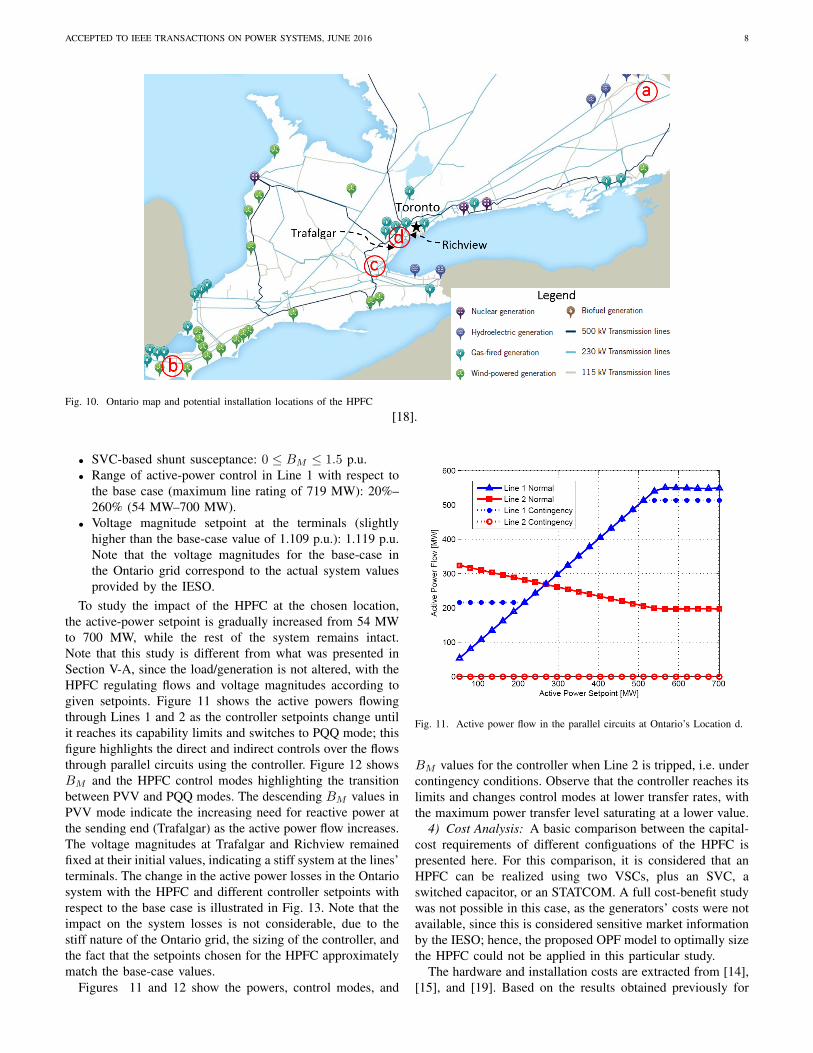
Fig. 10. Ontario map and potential installation locations of the HPFC[18].

• SVC-based shunt susceptance: 0 ≤ BM ≤ 1.5 p.u.• Range of active-power control in Line 1 with respect to

the base case (maximum line rating of 719 MW): 20%–260% (54 MW–700 MW).

• Voltage magnitude setpoint at the terminals (slightlyhigher than the base-case value of 1.109 p.u.): 1.119 p.u.Note that the voltage magnitudes for the base-case inthe Ontario grid correspond to the actual system valuesprovided by the IESO.

To study the impact of the HPFC at the chosen location,the active-power setpoint is gradually increased from 54 MWto 700 MW, while the rest of the system remains intact.Note that this study is different from what was presented inSection V-A, since the load/generation is not altered, with theHPFC regulating flows and voltage magnitudes according togiven setpoints. Figure 11 shows the active powers flowingthrough Lines 1 and 2 as the controller setpoints change untilit reaches its capability limits and switches to PQQ mode; thisfigure highlights the direct and indirect controls over the flowsthrough parallel circuits using the controller. Figure 12 showsBM and the HPFC control modes highlighting the transitionbetween PVV and PQQ modes. The descending BM values inPVV mode indicate the increasing need for reactive power atthe sending end (Trafalgar) as the active power flow increases.The voltage magnitudes at Trafalgar and Richview remainedfixed at their initial values, indicating a stiff system at the lines’terminals. The change in the active power losses in the Ontariosystem with the HPFC and different controller setpoints withrespect to the base case is illustrated in Fig. 13. Note that theimpact on the system losses is not considerable, due to thestiff nature of the Ontario grid, the sizing of the controller, andthe fact that the setpoints chosen for the HPFC approximatelymatch the base-case values.

Figures 11 and 12 show the powers, control modes, and

Fig. 11. Active power flow in the parallel circuits at Ontario’s Location d.

BM values for the controller when Line 2 is tripped, i.e. undercontingency conditions. Observe that the controller reaches itslimits and changes control modes at lower transfer rates, withthe maximum power transfer level saturating at a lower value.

4) Cost Analysis: A basic comparison between the capital-cost requirements of different configuations of the HPFC ispresented here. For this comparison, it is considered that anHPFC can be realized using two VSCs, plus an SVC, aswitched capacitor, or an STATCOM. A full cost-benefit studywas not possible in this case, as the generators’ costs were notavailable, since this is considered sensitive market informationby the IESO; hence, the proposed OPF model to optimally sizethe HPFC could not be applied in this particular study.

The hardware and installation costs are extracted from [14],[15], and [19]. Based on the results obtained previously for


Fig. 12. HPFC control modes and BM as the loading level increases under:(a) normal, and (b) contingency conditions.

Fig. 13. Change in active power loss in the system with the HPFC withrespect to the base case.

different desired control ranges, under normal conditions, onecan obtain the controller ratings; thus, for example, for a400 MW power transfer limit, the converter current ratingswould be approximately 3.75 p.u., whereas the voltage ratingswould correspond to 0.022 p.u., and BM would be 1.21 p.u.from Fig. 12. Figure 14 shows the capital cost requirementswith respect to the power ratings for the HPFC with differentconfigurations for its shunt component, namely, an SVC withan 80 MVAr fixed capacitor, an equivalent switched capacitorbank, and an equivalent STATCOM; observe the significantcost advantages of the HPFC with shunt capacitor banks orSVC.

VI. CONCLUSIONS

Steady-state models of the HPFC for power flow andoptimal power flow studies have been proposed in this paper,considering the device’s various control modes. A strategy forhandling the violated constraints in power flow calculationshas been considered, and an optimal dispatch of the device in

Fig. 14. Capital costs of the HPFC with different shunt components fordifferent control ranges.

the system was examined within an OPF context, consideringrelevant operational constraints, to determine its optimal sizeand setpoints. The models were validated and tested using atwo-area benchmark test system, and their practical applicationand advantages were demonstrated in Ontario-Canada’s grid.From the presented studies, it can be concluded that the HPFCis an attractive option for congestion relief in real powernetworks.

ACKNOWLEDGMENTS

The authors would like to thank Dr. Jovan Bebic of GEEnergy Consulting, USA, for his insightful comments andsuggestions, and the IESO for their valuable input.

REFERENCES

[1] X. P. Zhang, C. Rehtanz, and B. Pal, Flexible ac Transmission Systems,Modelling and Control. Berlin, Germany: Springer 2006.

[2] I. Axente, R. K. Varma, and W. Litzenberger, “Bibliography of FACTS:2000 – part I IEEE working group report,” in Proc. IEEE PES GeneralMeeting, pp. 1–6, 2011.

[3] S. Arabi, P. Kundur, and R. Adapa, “Innovative techniques in modelingUPFC for power system analysis,” IEEE Trans. Power Syst., vol. 15,no. 1, pp. 336-341, Feb. 2000.

[4] S. Zelingher, B. Fardanesh, B. Shperling, S. Dave, L. Kovalsky,C. Schauder, and A. Edris, “Convertible Static Compensator project- hardware overview,” in Proc. IEEE PES Winter Meeting, vol. 4,pp. 2511–2517, 2000.

[5] J. Z. Bebic, P. W. Lehn, and M. R. Iravani, “The Hybrid Power FlowController - a new concept for flexible ac transmission,” in Proc. IEEEPES General Meeting, Montreal, Quebec, Canada, pp. 1–8, 2006.

[6] V. K. Sood and S. D. Sivadas, “Simulation of Hybrid Power FlowController,” in Proc. Int. Conf. Power Electronics, Drives and EnergySystems (PEDES) & Power India, pp. 1–5, Dec. 2010.

[7] N. R. Merritt and D. Chatterjee, “Performance improvement of powersystems using Hybrid Power Flow Controller,” in Proc. Int. Conf. Powerand Energy Systems (ICPS), pp. 1–6, Dec. 2011.

[8] A. G. Exposito, A. J. Conejo, and C. Canizares, Electric Energy Systems,Analysis and Operation. Boca Raton, FL., USA: CRC Press, 2009.

[9] F. Milano, “An open source power system analysis toolbox,” IEEE Trans.Power Syst., Vol. 20, No. 3, pp. 1199-1206, Aug. 2005.

[10] R. Fourer, D. Gay, and B. Kernighan, AMPL: A Modeling Language forMathematical Programming. Pacific Grove, CA., USA: McGraw-Hill,2003.

[11] PSSrE 33, Program Application Guide, 2013.


[12] Python, Program Website, [Online]. Available: https://www.python.org/[13] P. Kundur, Power System Stability and Control. New York: McGraw-

Hill, 1994.[14] M. Eslami, H. Shareef, A. Mohamed, and M. Khajehzadeh, “A survey

on Flexible AC Transmission Systems (FACTS),” Przeglad Elektrotech-niczny, Issue 01a, pp. 1–11, Jan. 2012.

[15] “Flexible AC Transmission Systems benefits study,” San Diego Gas andElectric, San Deigo, CA., USA, Oct. 1999.

[16] “18-month outlook,” Ontario Independent Electricity System Operator(IESO), Public report, May 2010 [Online]. Available: http://www.ieso.ca

[17] Ontario Independent Electricity System Operator (IESO), [Online].Available: http://www.ieso.ca

[18] Ontario Energy Report [Online]. Available:http://www.ontarioenergyreport.ca/

[19] R. M. Mathur and R. K. Varma, Thyristor-based FACTS Controllers forElectrical Transmission Systems. New York: John Wiley & Sons, 2002.

Behnam Tamimi (S05) received the B.Sc. degreein Electronics Engineering from the University ofTehran, Tehran, Iran, in 2001 and the M.Sc. de-gree in electrical engineering from KNT University,Tehran, in 2003. He is currently a PhD student atthe University of Waterloo, Canada. He has beena member of two IEEE-PES taskforces on bench-marking test systems for stability analysis. His re-search interests include power system analysis in thecontext of liberalized markets, and power electronicsapplications in power systems.

Claudio Canizares (S86, M91, SM00, F07) is aProfessor at the University of Waterloo since 1993and currently serves as the Hydro One EndowedChair and the Associate Chair for Research of theECE Department. His highly cited research activitiesfocus on the study of modeling, simulation, com-putation, stability, control, and optimization issuesin power and energy systems in the context ofcompetitive energy markets and smart grids. He is aFellow of the IEEE, of the Royal Society of Canada,and of the Canadian Academy of Engineering, and

the recipient of the 2016 IEEE Canada Electric Power Medal and of othervarious awards and recognitions from IEEE-PES Technical Committees andWorking Groups, where he has held several leadership positions.

Claudia Battistelli (M08) received her MS (2006)and PhD (2010) degrees in Electrical Engineeringfrom the Federico II University of Naples, Italy.She was at the Electrical and Computer EngineeringDepartment of the University of Waterloo, Canada,as a visiting PhD student in May 2008-Apr. 2009,and as a Postdoctoral Fellow in Jan.-Dec. 2013.Since Jan. 2014, she works as a Research Associateat the Electrical and Electronic Engineering Depart-ment of Imperial College, London, UK. Her researchareas include mathematical optimization techniques,

power systems analysis, and sustainable power and energy systems in theSmart Grid context.

accepted to ieee transactions on power … · sator (statcom), the series static ... savings stem...

Documents