Introduction Preliminary Our Approach Empirical Analysis Conclusion & Future Work

Accelerating Online CP Decompositions for

Higher Order Tensors

Shuo Zhou1, Nguyen Xuan Vinh1, James Bailey1,Yunzhe Jia1 and Ian Davidson2

1The University of Melbourne2University of California, Davis

KDD’2016

Introduction Preliminary Our Approach Empirical Analysis Conclusion & Future Work

1 Introduction

2 Preliminary

3 Our Approach

4 Empirical Analysis

5 Conclusion & Future Work

Introduction Preliminary Our Approach Empirical Analysis Conclusion & Future Work

Introduction

Introduction Preliminary Our Approach Empirical Analysis Conclusion & Future Work

Motivation

Multi-way structure→ How to represent it?

Highly complex data→ How to simplify it?

New data keeps arriving→ How to learn online?

Introduction Preliminary Our Approach Empirical Analysis Conclusion & Future Work

Tensor

Tensor (multi-way array) is a natural representation formulti-dimensional data, e.g. videos, time-evolving networks

Introduction Preliminary Our Approach Empirical Analysis Conclusion & Future Work

CP Decomposition

Introduction Preliminary Our Approach Empirical Analysis Conclusion & Future Work

2.492 2.493 2.494 2.495 2.496 2.497 2.498 2.499 2.5

x 106

2.407

2.408

2.409

2.41

2.411

2.412

2.413x 10

6 Spatial Activations Above Mean Factor 1

0600 0900 1200 1500 1800 2100 00000.04

0.06

0.08

0.1

0.12

0.14

0.16Temporal Activations Above Mean Factor 1

2.492 2.493 2.494 2.495 2.496 2.497 2.498 2.499 2.5

x 106

2.407

2.408

2.409

2.41

2.411

2.412

2.413x 10

6 Spatial Activations Above Mean Factor 2

0600 0900 1200 1500 1800 2100 0000−0.2

−0.1

0

0.1

0.2

0.3

0.4

0.5Temporal Activations Above Mean Factor 2

CP decomposition is a method to simplify and summarizetensors

1X. N.Vinh, J. Chan, I. Davidson, Simplifying Spatial Temporal Event Objects into Dictionaries

Introduction Preliminary Our Approach Empirical Analysis Conclusion & Future Work

But, online?

Introduction Preliminary Our Approach Empirical Analysis Conclusion & Future Work

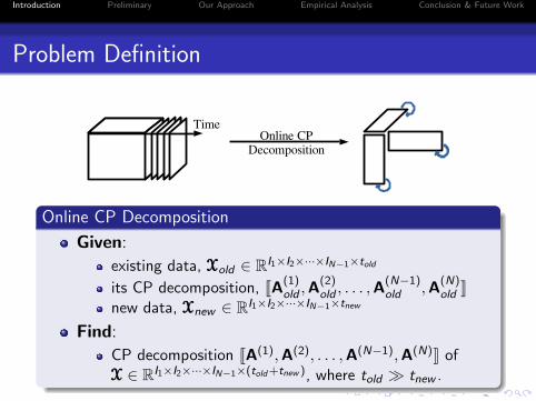
Problem Definition

Online CP Decomposition

Given:

existing data, XXXold ∈ RI1×I2×···×IN−1×told

its CP decomposition, JA(1)old ,A

(2)old , . . . ,A

(N−1)old ,A

(N)old K

new data, XXXnew ∈ RI1×I2×···×IN−1×tnew

Find:

CP decomposition JA(1),A(2), . . . ,A(N−1),A(N)K ofXXX ∈ RI1×I2×···×IN−1×(told+tnew ), where told � tnew .

Introduction Preliminary Our Approach Empirical Analysis Conclusion & Future Work

Preliminary

Introduction Preliminary Our Approach Empirical Analysis Conclusion & Future Work

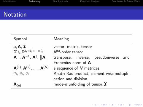
Notation

Symbol Meaning

a,A,XXX vector, matrix, tensorXXX ∈ RI1×I2×···×IN Nth-order tensorA>, A−1, A†,

∥∥A∥∥ transpose, inverse, pseudoinverse and

Frobenius norm of AA(1),A(2), . . . ,A(N) a sequence of N matrices�, ~, � Khatri-Rao product, element-wise multipli-

cation and divisionX(n) mode-n unfolding of tensor XXX

Introduction Preliminary Our Approach Empirical Analysis Conclusion & Future Work

CP Decomposition

X(1) ≈ A(C� B)>

X(2) ≈ B(C� A)>

X(3) ≈ C(B� A)>

Algorithm 1 CP-ALS1: initialize A,B,C2: repeat

3: arg minA12

∥∥X(1) − A(C� B)>∥∥2

4: arg minB12

∥∥X(2) − B(C� A)>∥∥2

5: arg minC12

∥∥X(3) − C(B� A)>∥∥2

6: until converged

Introduction Preliminary Our Approach Empirical Analysis Conclusion & Future Work

Online CP Decomposition

Batch [3]

initialize with previous decompositionstill computationally expensivepoor scalability

SDT and RLST [6]

online tensor decomposition → online matrixfactorizationwork on third-order tensors only

GridTF [7]

divide into small grids and decompose them in parallel

Introduction Preliminary Our Approach Empirical Analysis Conclusion & Future Work

Our Approach

Introduction Preliminary Our Approach Empirical Analysis Conclusion & Future Work

Main Idea

ALS like algorithm

for each non-temporal mode, complimentary matricesare used for storing useful information from previousdecomposition

complementary matrices are incrementally updated, andloading matrices are estimated based on them

Introduction Preliminary Our Approach Empirical Analysis Conclusion & Future Work

Update Time Mode

fix A and B, update C

C =

[Cold

Cnew

]=

[Cold

Xnew (3)((B� A)>)†

]

Introduction Preliminary Our Approach Empirical Analysis Conclusion & Future Work

Update Non-temporal Modes

fix B and C, update A

L =1

2

∥∥X(1) − A(C� B)>∥∥2

∂L∂A

= A(C� B)>(C� B)− X(1)(C� B)

A = (X(1)(C� B))((C� B)>(C� B))−1

= PQ−1

Introduction Preliminary Our Approach Empirical Analysis Conclusion & Future Work

Incremental Update

P = X(1)(C� B) Q = (C� B)>(C� B)

P← P + Xnew (1)(Cnew � B)

Q← Q + (Cnew � B)>(Cnew � B)

A← PQ−1

Introduction Preliminary Our Approach Empirical Analysis Conclusion & Future Work

Empirical Analysis

Introduction Preliminary Our Approach Empirical Analysis Conclusion & Future Work

Datasets

Datasets SizeSlice Size

SourceS =

∏N−1i=1 Ii

COIL-3D 128× 128× 240 16,384[5]

COIL-HD 64× 64× 25× 240 102,400DSA-3D 8× 45× 750 360

[1]DSA-HD 19× 8× 45× 750 6,840FACE-3D 112× 92× 400 10,304

[8]FACE-HD 28× 23× 16× 400 10,304FOG 10× 9× 1000 90 [2]GAS-3D 30× 8× 2970 240

[4]GAS-HD 30× 6× 8× 2970 1,440HAD-3D 14× 6× 500 64

[10]HAD-HD 14× 12× 5× 6× 500 3,840ROAD 4666× 96× 1826 447,936 [9]

Introduction Preliminary Our Approach Empirical Analysis Conclusion & Future Work

Baselines

Batch Cold: ALS in Tensor Toolbox [3].

Batch Hot: ALS + previous decomposition.

SDT

RLST

GridTF

Introduction Preliminary Our Approach Empirical Analysis Conclusion & Future Work

Setup

Procedure

20% initialization, rest added by sliceaveraging over 10 runs

Evaluation metrics

effectiveness:

fitness ,

1−

∥∥∥XXX−XXX

∥∥∥∥∥XXX∥∥× 100%

efficiency: running time in seconds

Introduction Preliminary Our Approach Empirical Analysis Conclusion & Future Work

Effectiveness

Batch methods always obtain the best fitness overall

OnlineCP shows comparable results as batch algorithms

Performance of other online algorithms are much worse

Introduction Preliminary Our Approach Empirical Analysis Conclusion & Future Work

Efficiency

Batch methods are extremely time-consuming

Improvement of GridTF is not significant

Both SDT and RLST show very good performance

OnlineCP is also quite efficient and significantly fasterthan batch methods

Introduction Preliminary Our Approach Empirical Analysis Conclusion & Future Work

Effectiveness & Efficiency

Compared to Batch Hot

Relative fitness:

OnlineCP (97%)

RLST (76%)

GridTF (68%)

SDT (67%)

Speedup:

OnlineCP (555.59)

RLST (113.75)

SDT (93.56)

GridTF (1.75)

Introduction Preliminary Our Approach Empirical Analysis Conclusion & Future Work

Sensitivity to Initialization

XXX ∈ R20×20×100

best ALS fitness: 90.14%

200 trails of ALS initializationwith ε ∈ [9e − 1, 1e − 4]

initial fitness: 65.78± 15.3704

Final Fitness

Batch Hot 82.57±10.1474SDT 7.68±55.5205RLST 33.15±36.9270GridTF 57.43±15.2148OnlineCP 67.67±12.9846

Introduction Preliminary Our Approach Empirical Analysis Conclusion & Future Work

Scalability – Time

XXX ∈ R20×20×105

Length of Time Mode ×104

0 2 4 6 8 10

Ru

nn

ing

Tim

e

10-4

10-3

10-2

10-1

100

101

Batch Hot

SDT

RLST

GridTF

GridTF-update

OnlineCP

(a) Log scale

Length of Time Mode ×104

0 2 4 6 8 10

Ru

nn

ing

Tim

e

0

0.005

0.01

0.015

0.02

0.025

SDT

RLST

GridTF

GridTF-update

OnlineCP

(b) Normal scale

Introduction Preliminary Our Approach Empirical Analysis Conclusion & Future Work

Scalability – Slice Size

100 timestamps, slice size [100, 9× 106]

Slice Size ×106

0 2 4 6 8 10

Runnin

g T

ime

10-4

10-2

100

102

Batch Hot

SDT

RLST

GridTF

OnlineCP

(a) Log scale

Slice Size ×106

0 2 4 6 8 10

Runnin

g T

ime

0

2

4

6

8

10

12

Batch Hot

SDT

RLST

GridTF

OnlineCP

(b) Normal scale

Introduction Preliminary Our Approach Empirical Analysis Conclusion & Future Work

Conclusion & Future Work

Introduction Preliminary Our Approach Empirical Analysis Conclusion & Future Work

In conclusion, OnlineCP:1 is applicable to both 3rd and higher order online tensors2 shows very good quality of decompositions and

significant improvement in efficiency3 outperforms existing online approaches in terms of

stability and scalability

Future work:1 applications2 dynamic tensors3 constrained online tensor decomposition

Introduction Preliminary Our Approach Empirical Analysis Conclusion & Future Work

PDF & Code: http://shuo-zhou.info

Introduction Preliminary Our Approach Empirical Analysis Conclusion & Future Work

References I

K. Altun, B. Barshan, and O. Tuncel.

Comparative study on classifying human activities with miniature inertial and magnetic sensors.Pattern Recognition, 43(10):3605–3620, 2010.

M. Bachlin, M. Plotnik, D. Roggen, I. Maidan, J. M. Hausdorff, N. Giladi, and G. Troster.

Wearable assistant for parkinson’s disease patients with the freezing of gait symptom.Information Technology in Biomedicine, IEEE Transactions on, 14(2):436–446, 2010.

B. W. Bader, T. G. Kolda, et al.

Matlab tensor toolbox version 2.6.Available online, February 2015.

J. Fonollosa, S. Sheik, R. Huerta, and S. Marco.

Reservoir computing compensates slow response of chemosensor arrays exposed to fast varying gasconcentrations in continuous monitoring.Sensors and Actuators B: Chemical, 215:618–629, 2015.

S. A. Nene, S. K. Nayar, H. Murase, et al.

Columbia object image library (coil-20).Technical report, technical report CUCS-005-96, 1996.

D. Nion and N. D. Sidiropoulos.

Adaptive algorithms to track the parafac decomposition of a third-order tensor.Signal Processing, IEEE Transactions on, 57(6):2299–2310, 2009.

Introduction Preliminary Our Approach Empirical Analysis Conclusion & Future Work

References II

A. H. Phan and A. Cichocki.

Parafac algorithms for large-scale problems.Neurocomputing, 74(11):1970–1984, 2011.

F. S. Samaria and A. C. Harter.

Parameterisation of a stochastic model for human face identification.In Applications of Computer Vision, 1994., Proceedings of the Second IEEE Workshop on, pages 138–142.IEEE, 1994.

F. Schimbinschi, X. V. Nguyen, J. Bailey, C. Leckie, H. Vu, and R. Kotagiri.

Traffic forecasting in complex urban networks: Leveraging big data and machine learning.In Big Data (Big Data), 2015 IEEE International Conference on, pages 1019–1024. IEEE, 2015.

M. Zhang and A. A. Sawchuk.

Usc-had: a daily activity dataset for ubiquitous activity recognition using wearable sensors.In Proceedings of the 2012 ACM Conference on Ubiquitous Computing, pages 1036–1043. ACM, 2012.

Q & A