abundant shale gas resources: long-term implications for … · the impact of shale gas resources...
TRANSCRIPT

Abundant Shale Gas Resources: Long-Term Implications for U.S. Natural Gas Markets
Stephen P.A. Brown and Alan J. Krupnick* 1 July 2010
Abstract: According to recent assessments, the United States has considerably more recoverable natural gas in shale formations than was previously thought. Such a development raises expectations that U.S. energy consumption will shift toward natural gas. To examine how the apparent abundance of natural gas and projected growth of its use might affect natural gas prices, production, and consumption, we use NEMS-RFF to model a number of scenarios—reflecting different perspectives on natural gas availability, the availability of competing resources, demand for natural gas, and climate policy—through 2030. We find that more abundant shale gas resources create an environment in which natural gas prices are likely to remain attractive to consumers—even as policy advances additional uses of natural gas to reduce carbon dioxide emissions and bolster energy security.
* Stephen Brown is a nonresident fellow at Resources for the Future (RFF) and Alan Krupnick is a senior fellow and research director at RFF. The authors thank Peter Balash, Tina Bowers, Kara Callahan, Joel Darmstadter, Ruud Egging, Bob Fri, Steve Gabriel, Less Goudarzi, Kristin Hayes, Hill Huntington, Karen Palmer, Ian Parry, Michael Schaal, Phil Sharp, Sharon Showalter, Dana Van-Wagener, Margaret Walls, John Weyant, Frances Wood, and participants in the May 20, 2010 meeting of the Task Force on Ensuring Stable Natural Gas Markets for helpful comments and discussions. Funding for this project was provided by the National Commission on Energy Policy. The views expressed are strictly those of the authors and do not necessarily represent those of RFF or the National Commission on Energy Policy.

2
1. Introduction
In recent years, the outlook for U.S. natural gas markets has changed dramatically. A
few years ago, most forecasts showed the United States growing increasingly dependent on
imports of liquefied natural gas (LNG). Now, the increased availability of domestic shale
gas resources promises dramatic changes in U.S. natural gas market conditions. Among the
projected changes are lower natural gas prices, increased self-sufficiency in natural gas,
and more opportunities to reduce carbon dioxide (CO2) emissions and increase energy
security by substituting natural gas for other fuels, such as coal and petroleum products.1
The characteristics of shale gas resources suggest the possibility of a substantial
change in U.S. natural gas supply (Figure 1). The higher quality shale gas basins provide
the low-cost portion of today’s North American natural gas supply and, overall, may make
the supply of natural gas more elastic than before. Consequently, more abundant shale gas
raises the possibility that domestic supply can meet considerable growth in U.S. natural gas
consumption over the next few decades without substantial gains in natural gas prices, and
with reduced reliance on LNG imports.
To investigate these possibilities, we examine seven scenarios that reflect different
perspectives on natural gas availability, market demand for natural gas, and policies that
would promote the use of natural gas (see Appendix). We modeled these scenarios, which
run through 2030, using NEMS-RFF.2 The scenarios reflect different perspectives on
1 See Brown et al. (2009) for a discussion of the implications of greater natural gas resources for a low-carbon future. 2 The National Energy Modeling System (NEMS) is a computer-based, energy-economy market equilibrium modeling system for the United States developed by the U.S. Department of Energy. NEMS-RFF is a version of NEMS developed by Resources for the Future in cooperation with OnLocation, Inc. NEMS-RFF projects market-clearing prices and quantities across a number of energy markets, subject to assumptions about macroeconomic and financial developments, world energy market conditions, demographics, resource

3
natural gas resources in shale formations, the adoption of low-carbon policies, the future
availability of nuclear and renewable power generation, the use of LNG-fueled heavy-duty
trucks, and industrial demand for natural gas. These scenarios are designed to examine
how natural gas production and prices will respond as market dynamics and/or policies
increase natural gas demand. Will prices rise sharply with strong gains in demand, or will
they remain relatively constant?
In the next section, we examine the potential role of shale gas in the evolution of U.S.
natural gas markets. In section 3, we use runs from NEMS-RFF to assess how abundant
natural gas and increased use of natural gas will interact to establish new market realities.
In section 4, we examine potential issues with our approach to modeling changes in U.S.
natural gas markets. Section 5 offers a summary and conclusion.
2. The Role of Shale Gas in U.S. Natural Gas Markets
Natural gas plays an important role in U.S. energy use. According to the U.S. Energy
Information Administration (EIA), natural gas accounted for nearly 25 percent of total U.S.
energy consumption in 2008. Only petroleum consumption accounted for more. In
contrast with oil and coal (the use of which are concentrated in transportation and
electricity, respectively), natural gas is used across a variety of sectors in the U.S. economy
(Figure 2). The industrial sector is the largest user, accounting for nearly 35 percent of
total natural gas consumption.3 The electricity sector accounts for nearly 30 percent.4 The
residential sector is the second-largest end-use sector, accounting for more than 20 percent
availability and costs, the cost and performance characteristics of energy technologies, and behavioral and technological choice criteria. 3 This figure includes lease and plant fuel. 4 Unlike the industrial, residential, commercial and transportation sectors, the electric sector is not an end-user of energy. It transforms energy from one form to another for use in the industrial, residential, commercial and transportation sectors.
4
of total natural gas consumption. Natural gas is also used in the commercial sector, and a
small amount of natural gas is used in the transportation sector.5
As shown in Figure 3, U.S. natural gas supplies come from a variety of sources,
including domestic production, imports through pipelines from Canada, and LNG from a
number of countries. Currently, almost 99 percent of U.S. gas consumption comes from
domestic sources and Canada.6 Under baseline projections from NEMS-RFF, which relies
on the conservative assumptions about shale gas resources embodied in the U.S. Energy
Information Administration’s Annual Energy Outlook 2009, hereafter identified as
“AEO2009” (EIA 2009), that percentage is expected to fall to slightly less than 97 percent in
2030 as the United States imports more LNG.
Over the same time horizon, U.S. natural gas production is expected to continue a
transition to unconventional sources, such as shale, coalbed methane, or tight sands. Arctic
production sites in Alaska and Canada’s Mackenzie Delta are also thought to be important
future sources of North American natural gas. Looking beyond 2030, gas hydrates may
contribute a significant share of U.S. natural gas production, and the production of coalbed
methane may expand considerably.
2.1 A Paradigm Shift in U.S. Natural Gas Supply
The impact of shale gas resources on the U.S. market is likely to prove more
substantial than the baseline projections show. In AEO2009, EIA placed U.S. shale
resources at 269.3 trillion cubic feet with total U.S. natural gas resources of 1,759.5 trillion
5 Some natural gas is used as a fuel for its own transportation in pipelines. 6 The United States also exports natural gas to Mexico, and that is projected to continue under all of the scenarios examined.

5
cubic feet.7 In contrast, the Potential Gas Committee (PGC 2009) provides an estimate of
615.9 trillion cubic feet.8 As shown in Figure 4, these shale gas resources are widely
distributed throughout the United States.
Natural gas has been produced for decades at low rates from shallow, fractured
shale formations in Appalachia, Michigan, and Colorado. The oil and gas industry also has
been long aware of the natural gas resources trapped in deep shale formations. Ranging
5,000 to 10,000 feet below the surface, deep shale gas formations are characterized by a
low permeability that naturally impedes the flow of natural gas out of the formation
through the borehole to the surface.
Although the industry only began to realize in late 2008 to what extent the
paradigm had shifted, the change in U.S. natural gas markets began more than a decade ago
with the gradual development of new technology. Low-cost coalbed methane in the San
Juan Basin of Colorado and New Mexico was first. Next came new techniques for the
development and production of natural gas in tight sand formations in western Wyoming.
The big shift came with the emergence of the Barnett shale in Texas, quickly followed by
other shale gas formations such as Horn River (British Columbia), Marcellus (Pennsylvania,
New York, and West Virginia), and Haynesville (Arkansas).
A new combination of horizontal drilling and hydraulic fracturing greatly increases
the permeability of deep shale gas formations, yields high rates of natural gas production,
and lowers costs. Horizontal drilling is accomplished by first drilling downward and then
turning to create a long horizontal bore through the shale formations holding the natural
7 AEO2010 (EIA 2010) expands the gas resource base to 317 trillion cubic feet. 8 An industry survey conducted by Navigant Consulting (2008) found that U.S. shale gas resources could be as great as 842 trillion cubic feet.

6
gas. This horizontal borehole increases exposure of the resource to an outward passage.
Hydraulic fracturing—which is most commonly accomplished by forcing a combination of
water, sand, and organic chemicals into the borehole—further opens up the structure to
increase flow of natural gas toward the horizontal borehole. Today shale gas formations
are regarded as among the largest and least costly U.S. sources of natural gas (Figure 5).9
3. Abundant Supply and Increased Demand: Assessing the Interaction
To evaluate how more abundant natural gas from shale deposits and increased
natural gas demand work together to affect U.S. energy markets, we use NEMS-RFF to
develop a number of scenarios. As shown in Figure 6, NEMS-RFF comprises 13 separate
modules that are run interactively to develop scenarios with market-clearing prices and
quantities across all U.S. energy markets.
The scenarios start with a business-as-usual case without abundant shale gas
resources, continue through a case with more abundant shale gas resources, and then
proceed to cases in which policy alters natural gas demand. These latter cases allow us to
examine how changes in demand interact with more abundant shale gas resources and
assess whether natural gas prices will rise sharply or remain relatively stable as policy or
changes in market conditions drive strong growth in demand.
3.1 The Baseline Case (Scenario 1)
The baseline scenario (Scenario 1) represents business as usual. It is based on
AEO2009 as revised in April 2009 to include energy provisions in the stimulus package
(EIA 2009). It also advances the implementation of more stringent corporate average fuel
economy standards from 2020 to 2016, as required by an Obama executive order issued in
9 All this could change to some extent depending on the resolution of regulatory issues associated with hydraulic fracturing.

7
May 2009. Following estimates from AEO2009, the baseline scenario assumes U.S. shale
natural gas resources of 269.3 trillion cubic feet with total U.S. natural gas resources of
1,759.5 trillion cubic feet.
Under Scenario 1, U.S. natural gas consumption is projected to grow insignificantly
from 2008 to 2030. Moreover, the projection shows natural gas consumption falling
through 2014, particularly in electricity generation, because recent changes in regulation
are expected to result in renewable energy, coal, and nuclear power to continue crowding
out natural gas.10 After 2014, the adjustment to regulatory change is mostly complete, and
the electric power sector shows increasing use of natural gas.
3.2 Some Implications of Abundant Natural Gas Supply (Scenario 2)
EIA’s estimates of U.S. natural gas supplies in AEO2009 date from 2007. To examine
the implications of more abundant shale gas resources, we replaced the EIA estimates with
those from the PGC (2009) to create Scenario 2. The PGC uses primary data sources to
estimate potential gas resources, and previous PGC estimates have been used in EIA
analyses. PGC puts these shale resources at 615.9 trillion cubic feet. We assume that this
increase in resources means that more natural gas can be produced from each well. This
approach yields both increased shale gas resources and lower production costs, which is
consistent with the industry’s perspective about the technological change.11 With higher
shale resources, total U.S. natural gas resources are boosted to 2,106.1 trillion cubic feet.
10 If capital costs for power plants are higher than assumed, the power sector will use more natural gas than the baseline case shows because coal, nuclear, and renewable power generation are more capital intensive than natural gas. 11 A more conservative approach of increasing basin size or areas would capture increased resources but not reduced costs.

8
With this change, U.S. natural gas production is much greater than in Scenario 1
(Figure 7). U.S. natural gas production shows only a mild decline from 2009 to 2014, with
steady gains coming after that. With additional natural gas supplies, natural gas prices are
lower—with the sharpest differences projected after 2025 (Figure 8). By 2030, the
projections show Henry Hub natural gas prices12 more than 20 percent lower than in
Scenario 1, falling from $8.81 per million British thermal units (Btu) to $6.86. Lower
natural gas prices delay the development of a natural gas pipeline from Alaska to the lower
48 states by three years and lead to 1.0 trillion cubic feet less offshore production in 2030.
Net imports (which combine LNG and pipeline imports with pipeline exports) total 0.39
trillion cubic feet under Scenario 1 in 2030 but become net exports of 0.57 trillion cubic
feet under Scenario 2. Even with such secondary effects, the responsiveness of U.S. natural
gas production to changes in price is greater than under Scenario 1.13
With more abundant supply, natural gas consumption is sharply higher than in
Scenario 1. The biggest difference in natural gas use between Scenarios 1 and 2 is found in
the electric power sector, where natural gas consumption is 22.5 percent higher in
Scenario 2 than in Scenario 1 (Table 1). Most of the gains in natural gas used in the electric
power sector come from substitution for other energy sources (Figure 9). Some of the
gains come from slightly increased electricity use brought about by lower electricity prices
(Table 2).
12 Near New Orleans, Henry Hub handles the highest volume of natural gas of any U.S. transportation node and is close to the largest concentration of natural gas–producing regions in the country. As such, Henry Hub is a commonly used pricing point for natural gas in the United States, and its price movements are highly correlated with the NYMEX futures price, which is the most widely traded natural gas contract in the world. 13 Estimates across the various scenarios show the model’s implied supply elasticity for domestic natural gas production in 2030 increases from 0.62 without abundant shale gas to 0.92–1.41 with abundant shale gas. Estimates of the implied elasticity of total natural gas supply (including imports) increase from 0.76 to 0.99–1.58.

9
3.3 Low-Carbon Policy without Abundant Natural Gas (Scenario 3)
Scenario 3 shows the effects of adopting a low-carbon policy in the absence of
abundant natural gas resources. The result is the introduction of a price wedge in the form
of a carbon allowance. The wedge drives down the Henry Hub price of natural gas while it
boosts the prices faced by end users (Figure 10).14 Because natural gas demand is
somewhat more inelastic than supply, consumers bear more of the wedge than producers
of natural gas.
As might be expected, the price movements have a considerable effect on U.S.
natural gas consumption (Figure 11). Coal and oil use are also reduced, but substantial
increases are found in the use of nuclear and renewable energy for power generation.15
Overall energy consumption is 5.4 percent lower in 2030, with electricity generation 8.2
percent lower than in Scenario 1. Energy consumption is lower in all sectors of the
economy, and CO2 emissions in 2030 fall from 6.2 billion tons in Scenario 1 to 4.8 billion
tons in Scenario 3.
In 2030, U.S. natural gas consumption is 1.67 trillion cubic feet (7.1 percent) lower
than in Scenario 1. For the same year, domestic natural gas production is 1.35 trillion cubic
feet (5.9 percent) lower. Imports are reduced slightly. As shown in Table 3, natural gas
consumption is lower in all major sectors of the economy in Scenario 3 than in Scenario 1.
The biggest reduction in natural gas use is in the electricity sector, where conservation and
gains in nuclear and renewable power generation displace natural gas and coal (Figure 12).
14 Similar wedges are found for coal, petroleum, and biofuels. 15 To recognize the political realities of opposition to the further development of nuclear power, we imposed limits on its growth of no more than 50 gigawatts of new capacity by 2030.

10
3.4 Low-Carbon Policy with Abundant Natural Gas (Scenario 4)
Scenario 4 shows the effects of adopting a low-carbon policy with abundant natural
gas resources. As with Scenario 3, the result is a price wedge in the form of a carbon
allowance. The wedge drives down the Henry Hub price of natural gas while boosting the
prices faced by end users (Figure 13).16 Because the elasticity of supply is increased by
abundant shale gas, producers bear less of the CO2 allowance, and those downstream from
Henry Hub absorb a greater share of the costs of a low-carbon policy. Nonetheless, the
price paid for natural gas plus the CO2 emissions allowances is lower than when natural gas
is less abundant. Abundant natural gas simply makes the price of natural gas lower, and
that effect dominates the results.
With abundant natural gas supplies (Scenarios 2 and 4), the implementation of a
cap-and-trade program yields a greater overall reduction in energy use than would occur
without abundant supplies (Scenarios 1 and 3). Because greater natural gas supplies foster
higher overall energy consumption and higher CO2 emissions in the absence of policy
intervention, bigger reductions in energy use are required to meet the CO2 emissions
targets (about 4.8 billion tons in 2030). Nonetheless, a comparison of differences between
Scenarios 2 and 4 and those of Scenarios 1 and 3 shows that total natural gas consumption
is only slightly reduced by the introduction of a low-carbon policy when natural gas
supplies are abundant (Figure 14).
In the process, the share of natural gas in electricity generation in 2030 rises from
23.9 to 27.8 percent when the low-carbon policy is implemented (Figure 15). That
16 Again, similar wedges are found for coal, petroleum, and biofuels.

11
contrasts with Scenario 3, which shows that the same low-carbon policy yields a decline in
the share of natural gas in electricity generation, from 19.4 percent to 18.8 percent. With
more abundant, less expensive natural gas supplies, the use of coal falls by more than when
natural gas is less abundant and less nuclear and renewable power is needed to meet CO2
emissions targets.17 In short, when natural gas supplies are more plentiful, market-based
policies to reduce CO2 emissions will yield a market-driven substitution of natural gas for
other fuels in the electric power sector.
The implementation of cap-and-trade policies increases electricity prices and
reduces electricity consumption (Table 4). Nonetheless, more abundant natural gas
resources change the realities of cap-and-trade policies. Electricity prices are lower and
electricity consumption is greater in Scenario 4 than in Scenario 3. The reduced use of coal
in the electricity sector and the increased substitution of electricity for other fuels in end-
use sectors yields the same CO2 emissions as found under Scenario 3.
Other sectors show limited substitution possibilities between natural gas and other
energy sources. As a consequence, more plentiful natural gas supplies do not lead to much
fuel switching, and emissions reductions in these sectors depend more heavily on energy
conservation. As a result, the implementation of a low-carbon policy slightly reduces
natural gas consumption in these sectors (Table 5).
3.5 Limits on Nuclear and Renewable Power Generation (Scenario 5)
Scenario 5 is designed to examine how limited deployment of nuclear and
renewable power generation might increase natural gas demand under climate policy. The
17 The limit of no more than 50 gigawatts of total growth in nuclear power capacity by 2030 is not binding in this scenario.

12
scenario is constructed by modifying Scenario 4. We place a limit of 30 gigawatts on
additions to nuclear power and restrict the growth rate of renewable power generation.18
These caps reflect a somewhat more pessimistic outlook for the use of these technologies than in
the first four cases—and may proxy the market penetration found with higher costs—but the
assumed costs for these technologies are not altered.19
The effects of limits on nuclear and renewable power generation are most apparent
in the electric power sector, where we see a substantial change in the sources of power
generation (Figure 16). As expected, nuclear and renewable energy play smaller roles in
the electric power sector and natural gas plays a larger role. Perhaps surprisingly, the use
of coal to produce electricity is also reduced. When zero-emissions technologies are less
available, it becomes more difficult to meet emissions targets. Cheap and dirty coal is
disadvantaged by the reduced availability of zero-emissions technologies, and its use must
be reduced. The advantage shifts to moderately clean but more expensive fuels, such as
natural gas.
Greater use of natural gas in the electric power sector increases overall natural gas
consumption and boosts natural gas prices (Figures 17 and 18). With somewhat higher
natural gas prices and limits on nuclear and renewable power generation, power
generation is more costly than in Scenario 4. Electricity prices are pushed upward slightly,
and overall electricity consumption is somewhat reduced (Table 6).
18 To create a case that examines the trade-off between electricity conservation and natural gas use, we also place restrictions on the use of additional carbon capture and storage to prevent the model from shifting in that direction. 19 Some estimate higher costs of nuclear power generation than assumed for the AEO2009, which provides the basic assumptions used in our analysis, but Rothwell (2010) finds them approximately correct.

13
Outside the electricity sector, higher natural gas prices amplify slightly what is
found in Scenario 4. In these sectors, natural gas consumption is reduced slightly below
that found in Scenario 4 (Table 7).
3.6 LNG Trucks with Abundant Natural Gas (Scenario 6)
Scenario 6 represents an aggressive penetration rate of new LNG-fueled heavy-duty
trucks (replacing new diesel-fueled trucks) combined with higher estimates of U.S. shale
resources.20 Based on Scenario 2, it models a 10 percent penetration of new LNG heavy-
duty (class 7 and 8) trucks beginning in 2011, rising over a 10-year period at an additional
10 percent per year each year, until 100 percent of new truck purchases are LNG-fueled by
2020. Although the scenario does yield reduced CO2 emissions in comparison to Scenario
2, it is designed to look at a policy that increases natural gas use without the
implementation of policy that specifically prices carbon.
The expanded use of natural gas vehicles (NGVs) in the United States is not unlikely.
Such vehicles have been a part of global vehicle fleets for decades, and the United States
ranks only twelfth globally in number of NGVs on the road. Most such vehicles in the
United States are city bus fleets and city-based truck fleets, such as Federal Express or
United Parcel Service, which can easily refuel at prescribed locations.
Limiting factors have included the high price differential between NGVs and their
diesel or gasoline counterparts, a relatively low and unstable price differential in favor of
natural gas as a fuel, the use of compressed natural gas as the fuel (which provides only a
20 Another potential way to use natural gas to replace petroleum consumption in the transportation sector is to substitute electric and hybrid-electric vehicles for a portion of the gasoline-powered light vehicles, and then use natural gas to produce the additional electricity. Such changes may necessitate technological gains and would likely require policy intervention in both transportation and electric power generation. Depending on the scale of implementation, the effects on oil and natural gas consumption could be similar to those for adoption of LNG vehicles. Obviously, the effects on electricity production and use would be considerable.

14
limited driving range), and a lack of a fueling infrastructure. With abundant supplies of
natural gas and the possibility of lower and more stable prices, the economics of NGVs may
improve. In addition, greater concerns about reducing oil consumption and greenhouse
gases provide further reasons for considering NGVs. Indeed, if broad-based carbon policies
are put in place, the lower carbon content of such fuels relative to gasoline or diesel may
further widen the price differentials in favor of natural gas.
One particular reason for optimism about the possibility of converting the heavy-
duty, long-haul truck fleet to be fueled by LNG is that such commercial vehicles are already
available and being used in the Port of Los Angeles. In addition, the differential between
the initial cost of a diesel truck and an LNG-fueled truck has been falling with technical
progress. Moreover, the increased development of systems to safely and efficiently use
LNG as the fuel for these vehicles means their driving range can be extended to be
comparable to diesel-fueled vehicles.
Infrastructure concerns also are diminishing as the long-haul trucking industry is
turning increasingly to a hub-and-spoke system with centralized drop-off/pick-up
locations, instead of relying on individual truckers to move goods fully across country.
Such a system enables gradual market penetration with LNG refueling taking place at a
limited number of hubs.
Krupnick (2010) used NEMS-RFF to examine the greenhouse gas, oil consumption,
and welfare cost implications of an aggressive penetration of new LNG-fueled heavy-duty
trucks beginning in 2011. Although NEMS-RFF doesn’t model penetration of NGVs, one can
think of the policy as a subsidy (or mandate) sufficient to bring about the 10 percent annual

15
penetration rate described above. By 2030, LNG trucks would make up about 70 percent of
the entire heavy-duty truck fleet under this “policy.”
As shown in Figure 19, the penetration of heavy-duty LNG trucks has a dramatic
effect on both diesel and natural gas use in the transportation sector. In the absence of LNG
trucks, diesel demand grows from slightly more than 5 quadrillion Btu to slightly more
than 6 quadrillion Btu, with negligible use of natural gas. With the penetration of LNG
trucks as specified above, diesel consumption is gradually eroded, until it is only 1.3
quadrillion Btu in 2030, with LNG taking its place and reaching about 4.2 quadrillion Btu in
2030.21
Although these shifts are quite large within the context of transportation fuels, they
are smaller with respect to the entire natural gas market. Primary energy consumption of
natural gas is 26.04 trillion cubic feet in 2030 without LNG trucks (Scenario 2) and 29.36
quadrillion Btu with them (Figure 20). Thus, it is not surprising that Henry Hub spot prices
are only 10 percent higher in 2020 and 8 percent higher in 2030 with the increased
demand from LNG trucks (Figure 21).
The effects are also seen in the electric power sector. As shown in Figure 22, higher
natural gas prices reduce its use in the electric power sector (compared with Scenario 2).
Increases in nuclear and renewable power make up for some of this decrease, but the end
result is slightly higher electricity prices and a slight reduction in overall electricity
consumption in comparison to Scenario 2 (Table 8).
21 Note that an overall small reduction in the consumption of the sum of both fuels in 2030 owes to complex interactions in the NEMS-RFF model.

16
3.7 Maximum Natural Gas Demand Growth with Abundant Natural Gas (Scenario 7)
Scenario 7 explores the consequences for the natural gas market, the electric power
sector, and other relevant parts of the energy market when the use of natural gas is
maximized as much as is reasonably plausible. This scenario explores the elasticity of
natural gas supply with greater shale gas resources. The increase in demand is generated
by four factors:
1. Cap-and-trade with the same limits as Scenario 4, but with the requirement that the CO2 reductions be met without contributions from the transportation sector to create more pressure on the other sectors, which rely more heavily on natural gas;
2. Limits on the growth of nuclear and renewable power generation, which may proxy higher costs, as in Scenario 5;
3. Aggressive LNG-fueled heavy-duty truck penetration as in Scenario 6; and 4. Stronger industrial growth in natural gas use than in the baseline case to offset the
conservative assumptions about industrial sector growth in AEO2009.
As shown in Figure 23, the maximum demand scenario yields the greatest natural
gas consumption of any of the scenarios, although by only 1.6 trillion cubic feet more in
2030 than found under Scenario 6 alone (Table 9). The moderate difference should not be
surprising because the competing increases in natural gas demand bid up prices and crowd
each other out to some degree. Nonetheless, the increase in natural gas consumption from
Scenario 2 to Scenario 7 (4.9 trillion cubic feet) is greater than the combined increases
from Scenario 2 to Scenario 5 (0.5 trillion cubic feet) and from Scenario 2 to Scenario 6 (3.3
trillion cubic feet). The bigger increase in natural gas consumption is mostly a result of the
increased growth of industrial natural gas demand.
The maximum demand scenario pushes natural gas prices above all the other
scenarios modeled with enhanced gas shale resources (Figure 24). Henry Hub prices are
projected at $7.77 per million Btu in 2030, compared to $7.40 (Scenario 6) and $6.99
(Scenario 5). With a cap-and-trade system in place, prices for fossil fuels are augmented by

17
the price of allowances in proportion to their carbon content. Because CO2 allowance
prices are higher in Scenario 7 compared to Scenario 5, the differential between Henry Hub
prices that include the allowance price ($1.45 per million Btu) is larger than the differential
in Henry Hub prices alone ($0.78 per million Btu).
As shown in Table 10, electricity prices are also highest under Scenario 7, reflecting
the higher price for natural gas and CO2 allowances. The higher electricity price induces
conservation; the total generation in this scenario is 4.5 terawatt hours, compared with 4.6
terawatt hours in the cap-and-trade Scenario 5 and 5.1 terawatt hours in Scenario 6.
The use of natural gas to generate electricity is also lower in Scenario 7 than in
Scenario 5—again because natural gas prices are higher. In comparison to Scenario 6,
however, the use of natural gas in Scenario 7 is higher because the cap-and-trade system
favors natural gas in electricity generation when shale gas is abundant and nuclear and
renewable power sources are limited (Figure 25).
3.8 Supply Curves
Finally, with all seven scenarios in place, we are much better able to assess how the
quantity of natural gas supplied to the market relates to its price. We have two supply
regimes (or supply curves) corresponding to different assumptions about shale gas
resources. Scenarios 1 and 3 represent the assumptions used in the AEO2009 in which
shale resources total 269.3 trillion cubic feet. Scenarios 2, 4, 5, 6, and 7 represent the 615.9
trillion cubic feet of shale resources estimated by the Potential Gas Committee. For
Scenarios 1 and 2, the quantity of natural gas supplied represents an equilibrium point
where the common demand curve (D) intersects the supply curves (S1 and S2). The

18
remaining scenarios are represented by shifts in the demand curve along the supply
curves.
These points are displayed in Figure 26, with the two supply curves and the original
demand curve drawn in. Although we only have two points to estimate the supply curve
corresponding to the AEO2009, the supply curve corresponding to the PGC (2009)
resource estimates is much lower and flatter. 22 A flatter supply curve is also revealed in
the implied elasticities of supply (Table 11), which show prices rising by a smaller
percentage than production as the latter is expanded from Scenario 2 to Scenario 7.
In general, our examination of the seven scenarios shows that when shale gas
resources are abundant, sizable increases in natural gas demand can be met while keeping
the projected Henry Hub price of natural gas below $8 per million Btu for 2030. This
aggressive case shows a 19 percent increase in natural gas consumption over a business-
as-usual case with abundant natural gas resources, yet the natural gas price rises by only
13 percent.23 Abundant shale gas resources create a situation in which natural gas prices
are likely to show long-run stability—even if future natural gas demand is much stronger
than currently projected.
3.8.1 The Composition of U.S. Natural Gas Production
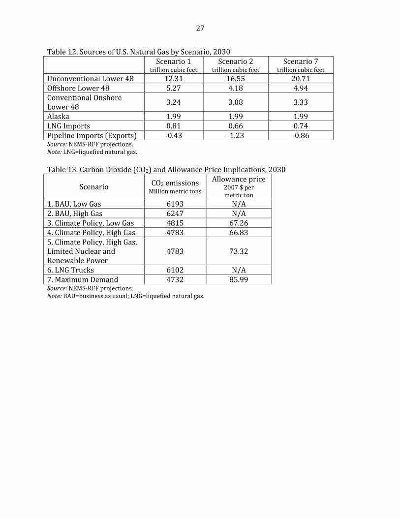
As shown in Table 12, additional shale gas resources yield a change in the
composition of U.S. natural gas supplies. Even in the absence of policies to increase natural
gas consumption (Scenario 2), production of unconventional natural gas increases
dramatically. Most other sources of U.S. natural gas production are reduced, with offshore
22 Krupnick (2010) also provides estimates for a scenario with LNG heavy-duty trucks and the AEO2009 gas resources. The 2030 Henry Hub price is $9.57 and consumption is 26.32 trillion cubic feet. Although unmarked, this point is approximately on the S1 curve as drawn. 23 The implied increase in demand is more than 25 percent.

19
production showing the biggest reduction. Being mostly an on-or-off proposition, the
quantity of Alaska production is unchanged. LNG imports are reduced, and net exports
through pipelines are increased. The latter is the result of reduced imports from Canada
and increased exports to Mexico.
As policy and other factors push natural gas consumption upward (Scenario 7), the
surge is met mostly with increases in unconventional natural gas. Other domestic sources
of natural gas also increase but remain lower than under Scenario 1. LNG imports are
pushed upward, and net exports are reduced.
3.9 CO2 Emissions
Much of the interest and excitement associated with shale gas involves its
implications for a low-carbon future. In this section, we examine the implications for
energy-related CO2 emissions and allowance prices (where applicable) in 2030 for all seven
scenarios (Table 13). We find that CO2 emissions with the PGC estimates of shale resources
(Scenario 2) are actually greater by 54 million metric tons in 2030 than for the case where
resources are far more limited (Scenario 1). Estimates for earlier years are similar.
Scenarios 3, 4, and 5 essentially set the same cap on CO2 emissions, although the
model yields different estimates for 2030 as the result of allowance banking. Climate
policies result in slightly lower allowance prices with the PGC resource estimates (Scenario
4) than with the AEO2009 estimates (Scenario 3), as noted above. Constraining renewable
and nuclear generation options forces greater reliance on natural gas, which raises
allowance prices (given the same cap).24
24 To the extent that the limits on renewable and nuclear generation proxy higher costs for their use, however, Scenario 5 would more accurately represent the costs of reducing CO2 emissions, and the estimated costs for Scenarios 3 and 4 would be much higher.

20
For Scenario 6 (LNG trucks), comparison with Scenario 2 shows an overall drop in
CO2 emissions of 145 million metric tons in 2030. This large drop is mostly the result of
natural gas replacing oil in transportation (for about a 20 percent drop in CO2 emissions
per Btu), and the higher price of natural gas discouraging use of this fuel in generation in
favor of renewable and nuclear power, as well as some coal.
Finally, the maximum demand case (Scenario 7) actually has the same cap on CO2 as
for Scenarios 3, 4, and 5, but without reliance on the transportation sector for any
reductions under the cap. As a result of the substitution of LNG for diesel in heavy trucks,
overall CO2 emissions are lower than for the other scenarios by about 50 million metric
tons in 2030. As might be expected, the allowance price is far higher under Scenario 7
because the mandated CO2 reductions must be obtained without any contributions from
the transportation sector, which pushes up costs in the remaining covered sectors.
4. Some Potential Issues with Our Analysis
In examining natural gas markets, a number of issues may arise that we did not
explicitly consider in our analysis. Such issues include changes in policy and technology,
including the possible elimination of oil and gas tax preferences, increased access to
moratoria lands in which natural gas production is currently limited, the potential for
increased production of coalbed methane, the potential availability of gas hydrates,
greater-than-projected Canadian natural gas exports, and less-than-projected exports to
Mexico. All these issues affect the outlook for U.S. natural gas markets but are likely to have
relatively little effect on the overall thrust of the present analysis; Brown et al. (2010)
suggest that the likely effects would be to increase the elasticity of supply, which would
further enhance price stability in U.S. natural gas markets.

21
In addition, the use of NEMS-RFF to assess the effects of more abundant shale gas
resources raises a question about how well the model captures the dynamics of U.S. natural
gas markets. Brown et al. (2010) find the issues most likely to have the biggest effects on
U.S. natural gas markets to be the projected growth of the industrial sector and the
substitution between natural gas and petroleum products in the industrial sector. Lesser
issues include pipeline capacity for the transportation of natural gas, the timing of the
development of a pipeline from Alaska to the lower 48 states, the potential for LNG exports
from Alaska, and the adequacy of U.S. LNG import terminals. We address the first two
issues by examining a case in which the industrial sector shows more rapid growth than
the baseline case.
Another concern is the extent to which the model reflects the costs of various
technologies for electricity generation. In particular, higher capital costs or higher
construction costs than are assumed in the model would disadvantage new coal, nuclear,
and renewable power generation facilities relative to those using natural gas. The limits
imposed on new nuclear and renewable power generation in Scenarios 5 and 7 may
approximate the effects higher capital costs on natural gas use in electricity generation.
5. Summary and Conclusions
New technology has provided a substantial increase in the quantity of natural gas
that can be produced from shale formations. Under business-as-usual scenarios, the NEMS-
RFF model shows that increased supply lowers projected natural gas prices by more than
20 percent in 2030. The prospect of plentiful and inexpensive domestic natural gas
increases the likelihood that changes in policy or market direction will lead to increased
natural gas demand.

22
In comparing scenarios with abundant shale gas resources, we find that a 19
percent increase in natural gas consumption above that currently projected for 2030 is
associated with an increase in the projected natural gas price of 13 percent. Moreover,
Scenario 7 (with abundant shale gas resources and 25 percent higher natural gas demand)
yields a projected natural gas price of $7.77 per million Btu at Henry Hub in 2030 and
natural gas consumption at 30.9 trillion cubic feet, while a scenario without abundant shale
gas resources but a strong demand increase related to LNG-fueled trucks yields a projected
price of $9.57 and natural gas consumption that is 4.6 trillion cubic feet lower (than
Scenario 7). In short, abundant shale gas resources provide an environment in which
relatively low U.S. natural gas prices seem likely to be sustainable over the long run.
The introduction of cap-and-trade polices will yield somewhat higher effective
natural gas prices for those using it as fuel than those found at Henry Hub because CO2
emissions allowances will need to be added to the price of natural gas. Under a policy
similar to (but with less generous offsets than) H.R. 2454, the Waxman-Markey cap-and-
trade bill that the House of Representatives passed last year, we find such allowances will
add another $3.54–4.56 per million Btu. With abundant shale gas resources, however, we
find that cap-and-trade policies increase the use of natural gas in the electric power sector,
as coal is more disadvantaged by the restrictions on carbon emissions. With or without
climate policy, an aggressive push on LNG trucks moderately lowers natural gas use in the
electric power sector.

23
References:
Brown, Stephen P.A., Steven A. Gabriel, and Ruud Egging. 2010. Abundant Shale Gas Resources: Some Implications for Energy Policy. Backgrounder. Washington, DC: Resources for the Future.
Brown, Stephen P.A., Alan J. Krupnick, and Margaret A. Walls. 2009. Natural Gas: A Bridge to a Low-Carbon Future? Issue brief 09-11. Washington, DC: Resources for the Future.
EIA (Energy Information Administration). 2009. Annual Energy Outlook 2009 (revised). Washington, DC: U.S. Department of Energy.
EIA. 2010. Annual Energy Outlook 2010. Washington, DC: U.S. Department of Energy. Krupnick, Alan J. 2010. Energy, Greenhouse Gas and Economic Implications of Natural Gas
Trucks. Backgrounder. Washington, DC: Resources for the Future. Navigant Consulting. 2008. North America Natural Gas Supply Assessment. Chicago, Illinois:
Navigant Consulting. PGC (Potential Gas Committee). 2009. Potential Supply of Natural Gas in the United States:
Advance Summary. Golden Colorado: Potential Gas Committee. Rothwell, Geoffrey. 2010. New U.S. Nuclear Generation: 2010–2030. Backgrounder.
Washington, DC: Resources for the Future.

24
Table 1. Natural Gas Consumption in 2030, by Selected Sector Scenario 1
trillion cubic feet Scenario 2
trillion cubic feet Difference Total 23.46 26.04 11.0% Electricity generation 6.71 8.23 22.5% Industrial natural gas use 6.29 6.89 9.5% Commercial natural gas use 3.43 3.63 5.8% Residential natural gas use 4.87 5.02 3.1% Source: NEMS-RFF projections.
Table 2. Average Electricity Price and Electricity Consumption, 2015–2030
Year
Prices Consumption Scenario 1 cents per KWh
Scenario 2 cents per KWh
Scenario 1 billion KWh
Scenario 2 billion KWh
2015 8.69 8.58 3,920 3,934 2020 9.28 8.99 4,125 4,157 2025 9.48 9.32 4,348 4,370 2030 10.04 9.31 4,527 4,604
Source: NEMS-RFF projections. Note: KWh=kilowatt hours.
Table 3. Natural Gas Consumption in 2030, by Selected Sector Scenario 1
trillion cubic feet Scenario 3
trillion cubic feet Difference Total 23.46 21.79 –7.1% Electricity generation 6.71 5.70 –15.1% Industrial natural gas use 6.29 6.06 –3.7% Commercial natural gas use 3.43 3.29 –4.1% Residential natural gas use 4.87 4.68 –3.9% Source: NEMS-RFF projections.
Table 4. Average Electricity Price and Electricity Consumption, 2015–2030
Year
Prices Consumption Scenario 2 cents per KWh
Scenario 3 cents per KWh
Scenario 4 cents per KWh
Scenario 2 billion KWh
Scenario 3 billion KWh
Scenario 4 billion KWh
2015 8.58 10.13 10.00 3,934 3,783 3,796 2020 8.99 11.02 10.75 4,157 3,937 3,960 2025 9.32 11.45 11.24 4,370 4,100 4,113 2030 9.31 12.75 12.36 4,604 4,171 4,199
Source: NEMS-RFF projections. Note: KWh=kilowatt hours.

25
Table 5. Natural Gas Consumption in 2030, by Selected Sector Scenario 2
trillion cubic feet Scenario 4
trillion cubic feet Difference Total 26.04 25.32 –2.8% Electricity generation 8.23 8.47 2.9% Industrial natural gas use 6.89 6.47 –6.2% Commercial natural gas use 3.63 3.39 –6.5% Residential natural gas use 5.02 4.77 –5.0% Source: NEMS-RFF projections.
Table 6. Average Electricity Price and Electricity Consumption, 2015–2030
Year
Prices Consumption Scenario 2 cents per KWh
Scenario 4 cents per KWh
Scenario 5 cents per KWh
Scenario 2 billion KWh
Scenario 4 billion KWh
Scenario 5 billion KWh
2015 8.58 10.00 10.23 3,934 3,796 3,775 2020 8.99 10.75 11.06 4,157 3,960 3,927 2025 9.32 11.24 11.56 4,370 4,113 4,078 2030 9.31 12.36 12.71 4,604 4,199 4,154
Source: NEMS-RFF projections. Note: KWh=kilowatt hours.
Table 7. Natural Gas Consumption in 2030, by Selected Sector Scenario 4
trillion cubic feet Scenario 5
trillion cubic feet Difference Total 25.32 26.53 4.8% Electricity generation 8.47 9.79 15.7% Industrial natural gas use 6.47 6.36 –1.8% Commercial natural gas use 3.39 3.36 –0.8% Residential natural gas use 4.77 4.73 –0.7% Source: NEMS-RFF projections.
Table 8. Average Electricity Price and Electricity Consumption, 2015–2030
Year
Prices Consumption Scenario 2 cents per KWh
Scenario 6 cents per KWh
Scenario 2 billion KWh
Scenario 6 billion KWh
2015 8.58 8.59 3,934 3,931 2020 8.99 9.15 4,157 4,138 2025 9.32 9.27 4,370 4,368 2030 9.31 9.55 4,604 4,583
Source: NEMS-RFF projections. Note: KWh=kilowatt hours.

26
Table 9. 2030 Natural Gas Quantities and Prices U.S.
consumption trillion cubic
feet
U.S. production trillion cubic
feet
Henry Hub price
2007 $ per million Btu
With CO2
allowance 2007 $ per million Btu
1. BAU, Low Gas 23.46 23.05 8.81 NA 2. BAU, High Gas 26.04 26.55 6.86 NA 3. Climate Policy, Low Gas 21.79 21.70 7.99 11.56 4. Climate Policy, High Gas 25.32 25.86 6.67 10.21 5. Climate Policy, High Gas, Limited Nuclear and Renewable Power
26.53 26.95 6.99 10.88
6. LNG Trucks 29.36 29.55 7.40 NA 7. Maximum Demand 30.94 31.02 7.77 12.33 Source: NEMS-RFF projections. Note: CO2=carbon dioxide; Btu=British thermal unit: BAU=business as usual; LNG=liquefied natural gas.
Table 10. 2030 Electricity Market Quantities and Price Total
generation billion KWh
Natural gas generation billion KWh
Average price
2007 cents per KWh
1. BAU, Low Gas 5057.64 981.03 10.04 2. BAU, High Gas 5159.03 1233.41 9.31 3. Climate Policy, Low Gas 4640.18 871.89 12.75 4. Climate Policy, High Gas 4695.78 1305.27 12.36 5. Climate Policy, High Gas, Limited Nuclear and Renewable Power
4635.22 1526.82 12.71
6. LNG Trucks 5127.24 1168.43 9.55 7. Maximum Demand 4545.76 1455.03 13.61 Source: NEMS-RFF projections. Note: KWh=kilowatt hours; BAU=business as usual; LNG=liquefied natural gas.
Table 11. Implied Elasticity of Supply, 2030
Scenarios Domestic Supply Total Supply Low Gas—Scenarios 1 and 3 0.62 0.76 High Gas—Scenarios 2 and 4 0.92 0.99 High Gas—Scenarios 2 and 5 0.77 0.95 High Gas—Scenarios 2 and 6 1.41 1.58 High Gas—Scenarios 2 and 7 1.25 1.38 Source: NEMS-RFF projections.
27
Table 12. Sources of U.S. Natural Gas by Scenario, 2030 Scenario 1
trillion cubic feet Scenario 2
trillion cubic feet Scenario 7
trillion cubic feet Unconventional Lower 48 12.31 16.55 20.71 Offshore Lower 48 5.27 4.18 4.94 Conventional Onshore Lower 48
3.24 3.08 3.33
Alaska 1.99 1.99 1.99 LNG Imports 0.81 0.66 0.74 Pipeline Imports (Exports) -0.43 -1.23 -0.86 Source: NEMS-RFF projections. Note: LNG=liquefied natural gas. Table 13. Carbon Dioxide (CO2) and Allowance Price Implications, 2030
Scenario CO2 emissions Million metric tons
Allowance price 2007 $ per metric ton
1. BAU, Low Gas 6193 N/A 2. BAU, High Gas 6247 N/A 3. Climate Policy, Low Gas 4815 67.26 4. Climate Policy, High Gas 4783 66.83 5. Climate Policy, High Gas, Limited Nuclear and Renewable Power
4783 73.32
6. LNG Trucks 6102 N/A 7. Maximum Demand 4732 85.99 Source: NEMS-RFF projections. Note: BAU=business as usual; LNG=liquefied natural gas.

28

29
Figure 4. Shale Gas Resources, Lower 48 States

30
Figure 5. Cost of Supply vs. Production
Figure 6. A Representation of the NEMS-RFF Modules

31

32

33

34

35

36

37
0.00
1.00
2.00
3.00
4.00
5.00
6.00
7.00
2015 2020 2025 2030
Qu
ad
rill
ion
Btu
Figure 19. Heavy Duty Freight Truck Fuel Use
Scen 2 Diesel
Scen 2 Natural Gas
Scen 6 Diesel
Scen 6 Natural Gas

38

39

40
Figure 26.
2
3
4
56
7
0
1
2
3
4
5
6
7
8
9
10
0 5 10 15 20 25 30 35
He
nry
hu
b p
rice
$/
mm
btu
Quantity of Natural Gas (tcf)
Demand and Supply of Natural Gas in 2030; Scenario scatter
1
S1
S2
D

41
Appendix: The Seven Scenarios
Scenario 1 (BAU, Low Gas) represents business as usual with estimates of U.S. shale gas resources at 269.3 trillion cubic feet. This case is based on the Energy Information Administration’s Annual Energy Outlook 2009 as revised in April to include energy provisions in the stimulus package, but it pulls new corporate average fuel economy standards forward from 2020 to 2016. Scenario 2 (BAU, High Gas) represents business as usual with higher estimates of U.S. shale resources. It is based on Scenario 1 with Potential Gas Committee estimates of U.S. shale gas resources at 615.9 trillion cubic feet. Scenario 3 (Climate Policy, Low Gas) represents the implementation of a low-carbon policy with the low estimates of U.S. shale gas resources. It is based on Scenario 1 with a cap-and-trade policy with CO2 emissions targets similar to those proposed by the Obama administration prior to the U.N. climate conference in Copenhagen and in H.R. 2454, the Waxman–Markey cap-and-trade bill, but with one billion tons of offsets rather than the two billion allowed under Waxman-Markey. The scenario also has a limit on nuclear power of no more than 50 gigawatts of new capacity by 2030. Scenario 4 (Climate Policy, High Gas) represents the implementation of a low-carbon policy with the high estimates of U.S. shale gas resources. It is based on Scenario 2 with a cap-and-trade policy and limits on nuclear power as in Scenario 3. Scenario 5 (Climate Policy, High Gas, Limited Nuclear and Renewable Power) represents the implementation of a low-carbon policy with high estimates of U.S. shale gas resources and limits on the use of nuclear power, carbon capture and sequestration (CCS), and renewable power generation. These limits restrict the use of nuclear power to no more than 30 gigawatts of new capacity by 2030, the use of CCS to 2 gigawatts, and renewable power generation to no more than is found under Scenario 3. Scenario 5 is based on Scenario 4 with the restrictions described. Scenario 6 (LNG Trucks, High Gas) represents aggressive implementation of a policy to switch heavy trucks from diesel fuel to LNG combined with higher estimates of U.S. shale resources. It is based on Scenario 2 with a 10 percent penetration of new LNG heavy-duty (class 7 and 8) trucks beginning in 2011, rising over the 10-year period an additional 10 percent per year each year, until 100 percent of new truck purchases are LNG–fueled by 2020. Scenario 7 (Maximum Demand, High Gas) represents five factors that might greatly increase natural gas demand with the higher estimates of shale gas resources. It is based on Scenario 2 with a cap-and-trade policy that excludes the transportation sector, a ceiling on nuclear and renewable power generation as in Scenario 5, the aggressive penetration of LNG trucks as in Scenario 6, and stronger industrial growth.