Abstraction, Decomposition, Relevance

Coming to Grips with Complexity in Verification

Ken McMillan

Microsoft Research

Need for Formal Methods that Scale• We design complex computing systems by debugging

– Design something approximately correct– Fix it where it breaks (repeat)

• As a result, the primary task of design is actually verification– Verification consumes majority of resources in chip design– Cost of small errors is huge ($500M for one error in 1990’s)– Security vulnerabilities have enormous economic cost

• The ugly truth: we don’t know how to design correct systems– Correct design is one of the grand challenges of computing

• Verification by logical proof seems a natural candidate, but...– Constructing proofs of systems of realistic scale is an overwhelming task– Automation is clearly needed

Model Checking

yes!

no!

p

q

ModelChecker

p

q

SystemModel

G(p ) F q)LogicalSpecification

Counterexample

A great advantage of model checking is the ability to producebehavioral counterexamples to explain what is going wrong.

Temporal logic (LTL)

• A logical notation that allows to succinctly express relationships of events in time

• Temporal operators– “henceforth p”– “eventually p”– “p at the next time”– “p unless q”

𝑝 ¬𝑝 ¬𝑝 ¬𝑝 𝑝 𝑝 𝑝 ...

¬𝐺𝑝 𝐺𝑝 𝐺𝑝 𝐺𝑝¬𝐺𝑝 ¬𝐺𝑝 ¬𝐺𝑝

Types of temporal properties

• Safety (nothing bad happens) “mutual exclusion”

“ must hold until ”

• Liveness (something good happens)“if , eventually ”

• Fairness“if infinitely often , infinitely often ”

We will focus on safety properties.

Safety and reachability

I

States = valuations of state variablesTransitions = execution stepsInitial state(s)

F

Bad state(s)Breadth-first searchCounterexample!

Reachable state set

I

F

Remove the “bug”Breadth-first searchFixed point = reachable state set

Safety property verified!

Model checking is a little more complex than this, butreachability captures the essence for our purposes.

Model checking can find very subtle bugs in circuitsand protocols, but suffers from state explosion.

Symbolic Model Checking• Avoid building state graph by using succinct representation for large

sets

0 0 0 1 0 0 0 1 0 0 0 1 1 1 1 1

d d d d d d d d

c c c c

0 1

0 1 0 1

0 1 0 1 0 1 0 1

b b

a

Binary Decision Diagrams (Bryant)

0 1

d

c

01

0 1

0 1

b

a

0

1

Symbolic Model Checking• Avoid building state graph by using succinct representation for large

sets

Multiprocessor Cache Coherence Protocol

S/F network

protocol

host otherhostsAbstract

model

• Symbolic Model Checking detected very subtle bugs• Allowed scalable verification, avoiding state explosion

The Real World

• Must deal with order 100K state holding elements (registers)

• State space is exponential in the number of registers

• Software complexity is greater

How do we cope with the complexity of real systems?

To make model checking a useful tool for engineers, wehad to find ways to cut this problem down to size. To do this, we apply three key concepts: decomposition, abstraction and refinement.

Deep v. Shallow Properties• A property is shallow if, in some sense, you don’t have to know very

much information about the system to prove it.

Deep property: System implements x86

Shallow property: Bus bridge never drops transactions

• Our first job is to reduce a deep property to a multitude of shallow properties that we can handle by abstraction.

Functional Decomposition

S/F network

protocol

host otherhostsAbstract

model

CAM

TAB

LE

S

~30K lines of verilog

Shallow properties track individual transactions though RTL...

Abstraction• Problem: verify a shallow property of a very large system• Solution: Abstraction

– Extract just the facts about the system state that are relevant to the proving the shallow property.

• An abstraction is a restricted deduction system that focuses our reasoning on relevant facts, and thus makes proof easier.

Relevance and refinement• Problem: how do we decide what deductions are relevant?

– Is relevance even a well defined notion?• Relevance:

– A relevant deduction is one that is used in a simple proof of the desired property.

• Generalization principle:– Deductions used in the proof of special cases tend to be relevant to the

overall proof.

Proofs• A proof is a series of deductions, from premises to conclusions• Each deduction is an instance of an inference rule• Usually, we represent a proof as a tree...

P1 P2

P3 P4 P5

C

Premises

Conclusion

P1 P2

C

If the conclusion is “false”, the proof is a refutation

Inference rules• The inference rules depend on the theory we are reasoning in

p : p D

_

Resolution rule:

Boolean logic Linear arithmetic

x1 · y1

x2 · y2

x1+x2 · y1+y2

Sum rule:

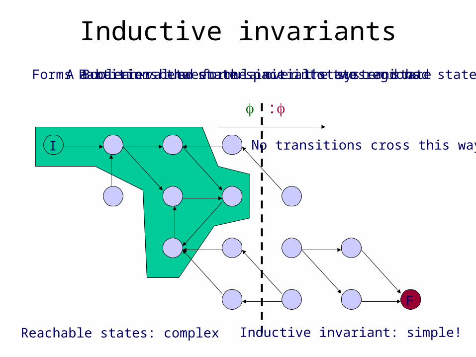
Reachable states: complex

Inductive invariants

I

F

A Boolean-valued formula over the system state

:

Partitions the state space into two regionsForms a barrier between the initial states and bad states

No transitions cross this way

Inductive invariant: simple!

Invariants and relevance• A predicate is relevant if it is used in a simple inductive invariant

l1: x = y = 0;l2: while(*)l3: x++, y++;l4: while(x != 0)l5: x--, y--;l6: assert (y == 0);

state variables: pc, x, y

inductive invariant = property +

pc = l1 Ç x = y

• Relevant predicates: pc = l1 and x = y

• Irrelevant (but provable) predicate: x ¸ 0

property: pc = l6 ) y = 0

Three ideas to take away• An abstraction is a restricted deduction system.• A proof decomposition divides a proof into shallow lemmas, where

shallow means "can be proved in a simple abstraction"• Relevant abstractions are discovered by generalizing from particular

cases.

These lectures are divided into three parts, covering these three ideas.

ABSTRACTION

What is Abstraction• By abstraction, we mean something like "reasoning with limited

information".• The purpose of abstraction is to let us ignore irrelevant details, and thus

simplify our reasoning.• In abstract interpretation, we think of an abstraction as a restricted

domain of information about the state of a system.• Here, we will take a slightly broader view:

An abstraction is a restricted deduction system

• We can think of an abstraction as a language for expressing facts, and a set of deduction rules for inferring conclusions in that language.

The function of abstraction• The function of abstraction is to reduce the cost of proof search by

reducing the space of proofs.

RichDeduction

System

Abstraction

Automated toolcan search this spacefor a proof.

• An abstraction is a way to express our knowledge of what deductions may be relevant to proving a particular fact.

Symbolic transition systems• Normally, we think of a discrete system as a state graph, with:

– a set of states – a set of initial states – a set of transitions .

• This defines a set of execution sequences of the system• It is often useful to represent and symbolically, as formulas:

• Note, we use for " at the next time", sot can be thought of as representing a set of pairs

• The system describe above has one execution sequence

Proof by Inductive Invariant• In a proof by inductive invariant, we prove a safety property according to

the following proof rule:

• This rule leaves great flexibility in choosing an abstraction (restricted deduction system). We can choose:

1. A language for expressing the inductive invariant .

2. A deductive system for proving the three obligations.

Many different choices have been made in practice. We will discussa few...

Abstraction languages• Difference bounds

is all conjunctions of constraints like and .

• Affine equalities

is all conjunctions of constraints .

• Houdini (given a fixed finite set of formulas

is all conjunctions of formulas in .

Abstraction languages• Predicate abstraction (given a fixed finite set of formulas

• Program invariants (given language of data predicates)

is all conjunctions of where .

is all Boolean combinations of formulas in .

Note

Example• Let's try some abstraction languages on an example...

l1: x = y = 0;l2: while(*)l3: x++, y++;l4: while(x != 0)l5: x--, y--;l6: assert (y == 0);

• Difference bounds• Affine equalities• Houdini with

(𝑝𝑐=𝑙2)⇒𝑥=𝑦(𝑝𝑐=𝑙3 )⇒𝑥=𝑦

Another example• Let's try an even simpler example...

l1: x = 0;l2: if(*)l3: x++;l4: elsel5: x--;l6: assert (x != 0);

• Difference bounds• Affine equalities• Houdini with

(𝑝𝑐=𝑙6 )⇒𝑥≥ −1∧𝑥≤1

(𝑝𝑐=𝑙2)⇒𝑥=0(𝑝𝑐=𝑙3 )⇒𝑥=0

(𝑝𝑐=𝑙5 )⇒ 𝑥=0(𝑝𝑐=𝑙6 )⇒𝑡𝑟𝑢𝑒

(𝑝𝑐=𝑙6 )⇒𝑡𝑟𝑢𝑒

• Predicate abstraction with

(𝑝𝑐=𝑙6 )⇒¬𝑥 ≤0∨¬𝑥≥0

Deduction systems• Up to now, we have implicitly assumed we have an oracle that can

prove any valid formulas of the forms:

• Thus, any valid inductive invariant can be proved. However, these proofs may be very costly, especially the consecution test . Moreover we may have to test a large number of candidates .

• For this reason, we may choose to use a more restricted deduction system. We will consider two cases of this idea:– Localization abstraction– The Boolean Programs abstraction

Localization abstraction• Suppose that where each is a fact about some system component.• We choose some subset of the 's that are considered relevant, and

allow ourselves any valid facts of the form:

• By restricting our prover to use only a subset of the available deductions, we reduce the space of proofs and make the proof search easier.

• If the proof fails, we may add components to .

𝜙∧𝑇⇒𝜙 ′

Example

Boolean Programs• Another way to restrict deductions is to reduce the space of conclusions.• The Boolean programs abstraction (as in SLAM) uses the same

language as predicate abstraction, but restricts deductions to the form:

where and

A Boolean program is defined by a set of such facts.

l1: int x = *;l2: if(x > 0){l3: x--;l4: assert(x >= 0);l5: }

Let

In practice, we may add some disjunctions to our setof allowed deductions, to avoid adding more predicates.

Proof search• Given a language for expressing invariants, and a deduction system for

proving them, how do we find a provable inductive invariant that proves a property ?

• Abstract interpretation– Iteratively constructs the strongest provable .– Independent of .

• Constraint-based methods– Set up constraint system defining valid induction proofs– Solve using a constraint solver– For example, abstract using linear inequalities and summation rule.

• Craig interpolation– Generalize the proofs of bounded behaviors

In general, making the space of proofs smaller will make the proofsearch easier.

Relevance and abstraction• The key to proving a property with abstraction is to choose a small

space of deductions that are relevant to the property.• How do we choose...

– Predicates for predicate abstraction?– System components for localization?– Disjunctions for Boolean programs?

• In the section on relevance, we will observe that deductions that are relevant to particular cases tend to be relevant in general. This gives us a methodology of abstraction refinement.

Next section: how to decompose big verification problemsinto small problems that can be proved with simple abstractions.

DECOMPOSITION

Proof decomposition• Our goal in proof decomposition is to reduce proof of a deep property of

a complex system to proofs of shallow lemmas that can be proved with simple abstractions.

• We will consider some basic strategies for decomposing a proof, and consider how they might affect the abstractions we need.

• We consider two basic categories of decomposition:– Non-temporal: reasoning about system states– Temporal: reasoning about sequences of states

• As we go along, we’ll look at a system called Cadence SMV that implements these proof decompositions, and corresponding abstractions.

Cadence SMV basics• Type declarations

• Variables and assignments

• Temporal assertions

typedef MyType 0..2;typedef MyArray array MyType of {0,1};

v : MyType;init(v) := 0;next(v) := 1 - v;

v = 0,1,0,1,0,...

p : assert G (v < 2);

SMV can automatically verify this assertion by model checking.

Case splitting• The simplest way to breakdown a proof is by cases:

• Here is a temporal version of case splitting:

p :p p :p :p p p

q q qq q q q

Temporal case splitting

Idea:let be most recent writer at time t.

p1 p2 p3 p4 p5

v1

...

f: I'm O.K. attime t.

• Here is a more general version of temporal case splitting:

Temporal case splitting in SMV

v : T;s : assert G p ;

forall (i in T) subcase c[i] of s for v = i;

c[0] : assert G (v=0 ) p) ;c[1] : assert G (v=1 ) p) ;...

Invariant decomposition• In a proof using an inductive invariant, we often decompose the

invariant into a conjunction of many smaller invariants that are mutually inductive:

{Á1 Æ Á2} s {Á1}{Á1 Æ Á2} s {Á2}

{Á1 Æ Á2} s {Á1 Æ Á2}

• To prove each conjunct inductive, we might use a different abstraction.• Often we need to strengthen an invariance property with many

additional invariants to make it inductive.

Á1 Æ Á2 Æ T ) Á’1Á1 Æ Á2 Æ T ) Á’2Á1 Æ Á2 Æ T ) Á’1 Æ Á’2

Temporal Invariant Decomposition• To prove a property holds at time t, we can assume that other properties

hold at times less than t. The properties then hold by mutual induction.• We can express this idea using the releases operator:

p q "p fails before q fails"

• If no property is the first to fail, then all properties are always true.

These premises can be checked with a model checker.

Invariant decomposition in SMV• This argument:

• can be expressed in SMV like this:

p : assert G ...;q : assert G ...;

using (p) prove q;using (q) prove p;

Combine with case splitting

p1 p2 p3 p4 p5

v1

...

f: I'm O.K. attime t.

To prove case at time , assume general case up to :

Combining in SMV• This argument:

• Can be expressed like this in SMV:

w : T;p : assert G ...;

forall(i in T) subcase c[i] of p for w = i;

forall(in in T) using (p) prove c[i];

Abstractions• Having decomposed a property into a collection of simpler properties,

we need an abstraction to prove each property.• Recall, an abstraction is just a restricted proof system.• SMV uses a very simple form of predicate abstraction called a data type

reduction.

• For data type T, pick a finite set of parameters • For each variable of type T, we allow predicates like .• For each array of type, say, we allow .

Data type abstraction

So the value of a variable in the abstraction is just or "other".The value of an array is known only at indices

Deduction rules• Recall that to describe an abstraction, we need to know not just the

abstract language (what can be expressed) but also what can be deduced.

• SMV's deduction rules are very weak. This table describes what SMV can deduce about the expression given the values of and of type , where is reduced with parameter set

𝑥=𝑦

𝑥=𝑖𝑥≠ 𝑖

𝑦=𝑖𝑦 ≠ 𝑖

1 00

When and are not , we can't deduce anything about .

Data type reductions in SMVThis code proves a property parameterize on by reducing data type to just the abstract values and .

typedef T 0..999;

forall(i in T) p[i] : assert G ...;

forall(i in T) using T -> {i} prove p[i];

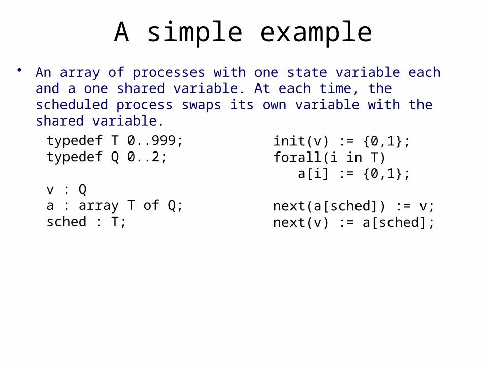
A simple example• An array of processes with one state variable each and a one shared

variable. At each time, the scheduled process swaps its own variable with the shared variable.

typedef T 0..999;typedef Q 0..2;

v : Qa : array T of Q;sched : T;

init(v) := {0,1};forall(i in T) a[i] := {0,1};

next(a[sched]) := v;next(v) := a[sched];

A simple example• We want to prove the shared variable always less than 2:

p : assert G (v < 2);

• Split cases on most recent writer of shared variable:

w : T;next(w) := sched;forall(i in T) subcase c[i] of p for w = i;

• Use mutual induction to prove the cases, with a data type reduction:

forall(i) using p, T->{i} prove c[i];

Functional decompositions• This combination of temporal case splitting and invariant decomposition

can support a general approach to decomposing proofs of complex systems.

• Use case splitting to divide the proof into “units of work” or "transactions". – For a CPU, this might be instructions, loads, stores, etc...– For a router, units of work might be packets.

• Each transaction can assume all earlier transactions are correct.• Since each unit of work uses only a small collection of system

resources, a simple abstraction will prove each.

Example : packet router

• Unit of work is a packet• Packets don’t interact• Each packet uses finite resources

– allows abstraction to finite state

Switchfabric

input buffers output buffers

Illustration: Tomasulo’s algorithm

• Execute instructions in data flow order

OP,DST

opra oprb

OP,DST

opra oprb

OP,DST

opra oprb

EU

EU

EU

OPS

TAGGED RESULTS

INSTRUCTIONS

VAL/TAGVAL/TAGVAL/TAGVAL/TAG

REGFILE

Data types in Tomasulo• The following data types are used in Tomasulo

– REG (register file indices)– TAG (reservation station indices)– EU (execution unit indices)– WORD (data words)

Specification via reference model

Referencemodel

System

SpecificationsInvariant properties specify values in the out-of-order system relative to the reference model.

Reference model describes simple in-order instruction execution.

Invariant decomposition

• Decompose into two lemmas

OP,DST

opra oprb

OP,DST

opra oprb

OP,DST

opra oprb

EU

EU

EU

OPS

TAGGED RESULTS

INSTRUCTIONS

VAL/TAGVAL/TAGVAL/TAGVAL/TAG

REGFILE

Lemma 1:Correct operands

Lemma 2:Correct results

"Correct" means same value as reference model computes.

Lemmas in SMV

• Lemma 1: The A operand in reservation station k is correct:

Note: only two system signals specified in proof decomposition

forall (k in TAG) lemma1[k] : assert G rs[k].valid & rs[k].opra.valid -> rs[k].opra.val = aux[k].opra;

• Lemma 2: Values on result bus with tag i are correct:

forall (i in TAG) lemma2[i] : assert G rb.tag = i & rb.valid ->

rb.val = aux[i].res;

Case splitting in Tomasulo

OP,DST

opra oprb

OP,DST

opra oprb

OP,DST

opra oprb

EU

EU

EU

OPS

INSTRUCTIONS

REGFILE

VAL/TAGVAL/TAGVAL/TAGVAL/TAG

TAGGED RESULTS

For each operand, split cases on the tag of the operand.

Proving Lemma 1• To prove correctness of operands, split cases on tag and reg:

forall (i in TAG; j in REG; k in TAG; d in WORD) subcase lemma1c[i][j][k][d] of lemma1[i] for rs[i].opra.tag = j & rs[i].tag = j & aux[i].opra = d;

• Then assume all results of earlier instructions are correct and reduce data types to just relevant values:

forall (i in TAG; j in REG; k in TAG; d in WORD) using (lemma2), TAG->{i,k}, REG->{j}, WORD->{d}, EU->{} prove lemma1c[i][j][k][d];

OP,DST

Uninterpreted functions• Verify Tomasulo for arbitrary EU function f(a,b).

f(a,b)

RESULTS

INSTRUCTIONS

SPEC

OP,DST

opra oprb

opra oprb

OP,DST

opra oprb

f(a,b)OPS

INSTRUCTIONS

REGFILE

VAL/TAGVAL/TAGVAL/TAGVAL/TAG

TAGGED RESULTS

f(a,b)

(related: Burch, Dill, Jones, etc...)

Case splitting for lemma 2• Break correctness of EU's into cases based on data values:

OP,DST

i j

OP,DST

opra oprb

OP,DST

opra oprb

f(a,b)

f(a,b)

f(a,b)

OPS

INSTRUCTIONS

REGFILE

VAL/TAGVAL/TAGVAL/TAGVAL/TAG

k

Result• SMV can reduce the verification of the lemmas to finite-state model

checking – Max 25 state bits to represent abstract values– Total verification time less than 4 seconds

• Tomasulo implementation proved for– Arbitrary number of registers, reservation stations– Arbitrary data word size and EU function

• (unbounded EU’s requires one more lemma)

Note the strategy we applied:1) Case split into "units of work" (operand fetch, result comp)2) Specify units of work relative to reference model3) Choose abstraction for each unit of work.

A more complex example

• Unit of work = instruction

OP,DST

opraoprb

OP,DST

opraoprb

OP,DST

opraoprb

EU

EU

EU

OPS

RETIRED RESULTS

INSTRUCTIONS

VAL/TAGVAL/TAGVAL/TAGVAL/TAG

REGFILE

BUF

BUF

BUF

RESPM

PC

branchpredictor

dec

LSQ DM

branch results

Scaling problem• Must consider up to three instructions:

– instruction we want to verify– up to two previous instructions

• Resulting abstractions too complex• Soln: break instruction execution into smaller units of work

– write more intermediate specifications• Compared to similar proof using manual inductive invariants...

– manual invariant proof approx. 2MB (!)– temporal decomposition and abstraction proof approx. 20 KB

64

Cache coherence (Eiriksson 98)

S/F network

protocol

hostprotocol

host

protocol

host

Distributedcachecoherence

INTF

P P

M IO

to net

• Nondeterministic abstract model• Atomic actions• Single address abstraction• Verified coherence, etc...

Mapping Protocol to RTL

S/F network

protocol

host otherhostsAbstract

model

CAM

TAB

LE

S

~30K lines of verilog

Shallow properties track individual transactions though RTL...

Conclusions• Proof decomposition means breaking down a proof into lemmas that

can be proved in simpler deduction systems (abstractions).• A functional decomposition approach divides the proof based on "units

of work" or "transactions".• This can be accomplished by two basic decomposition steps:

– Temporal case splitting– Temporal invariant decomposition

• Since each unit of work uses few resources, this style of decomposition lends itself to proof with fairly primitive abstractions, such as data type reductions.

Next section: more sophisticated abstractions and how wediscover them.

RELEVANCE

Relevance and Refinement• Having decomposed a verification problem into shallow temporal

lemmas, we need to choose an abstraction to prove each lemma.• That is, we are looking for a small space of relevant deductions in which

to search for a proof of a property.• In this section, we will focus on the question of how we determine what

is relevant and on how we apply this notion to the problem of abstraction refinement.

• Refinement is the process of choosing the deduction system that defines our abstraction. This is usually, but not always does as a process of gradual refinement of the abstraction, adding information until the property is proved.

Basic framework• Abstraction and refinement are proof systems

– spaces of possible proofs that we search

Abstractor

Refiner

General proof system

Incomplete

Specialized proof system

Complete

prog.

pf. special case cex.

pf. of special case

Refinement = augmenting abstractor’s proof system to replicateproof of special case generated by refiner.Narrow the abstractor’s proof space to relevant facts.

Background• Simple program statements (and their Hoare axioms)

{}[]{ ) }

{}x := e{[e/x]}

{}havoc x{8 x }

• A compound stmt is a sequence simple statements 1;...; k

• A CFG (program) is an NFA whose alphabet is compound statements.– The accepting states represent safety failures.

x = 0;while(*) x++;assert x >= 0;

[x<0]

x := x +1

x := 0

Hoare logic proofs• Write H(L) for the Hoare logic over logical language L.• A proof of program C in H(L) maps vertices of C to L such that:

– the initial vertex is labeled True– the accepting vertices are labeled False– every edge is a valid Hoare triple.

[x<0]

x := x +1

x := 0

{True} {False}{x ¸ 0}

This proves the failure vertex not reachable, orequivalently, no accepting path can be executed.

Path reductiveness• An abstraction is path-reductive if, whenever it fails to prove program C,

it also fails to prove some (finite) path of program C.

Example, H(L) is path-reductive if• L is finite• L closed under disjunction/conjunction

• Path reductiveness allows refinement by proof of paths.• In place of “path”, we could use other program fragments, including

restricted paths (with extra guards), paths with loops, procedure calls...• We will focus on paths for simplicity.

Example

x = y = 0;while(*) x++; y++;while(x != 0) x--; y--;assert (y == 0);

x:=0;y:=0

x:=x+1; y:=y+1

[x 0]; x:=x-1; y:=y-1

[x=0]; [y 0]

• Try to prove with predicate abstraction, with predicates {x=0,y=0}• Predicate abstraction with P is Hoare logic over the Boolean

combinations of P

{x=0 Æ y=0}

{x0 Æ y0}

{True}

{True}

{True}

{True}

{True}

{x = y}

{x = y}

{x = y}

{x = y}

{x = y}

{False}

{True}

Unprovable path

x = y = 0;

x++; y++;

x++; y++;

[x!=0];x--; y--;

[x!=0];x--; y--;

[x == 0][y != 0]

Cannot prove with PA({x=0,y=0})

Ask refiner to prove it!

Augment P with new predicate x=y.PA can replicate proof.

{x = y Æ x=0}

{x = y Æ x0}

{x = y}

{x = y}

{x = y}

{False}

{True}

Abstraction refinement:• Path unprovable to abstraction• Refiner proves• Abstraction replicates proof

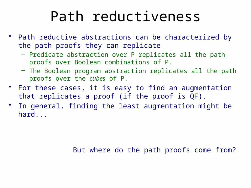
Path reductiveness• Path reductive abstractions can be characterized by the path proofs

they can replicate– Predicate abstraction over P replicates all the path proofs over Boolean

combinations of P.– The Boolean program abstraction replicates all the path proofs over the

cubes of P. • For these cases, it is easy to find an augmentation that replicates a

proof (if the proof is QF).• In general, finding the least augmentation might be hard...

But where do the path proofs come from?

Refinement methods

• Strongest postcondition (SLAM1)• Weakest precondition (Magic,FSoft,Yogi)• Interpolant methods

– Feasible interpolation (BLAST, IMPACT)– Bounded provers (SATABS)– Constraint-based (ARMC)

Local proof

Interpolation Lemma

• If A Ù B = false, there exists an interpolant A' for (A,B) such that:

A Þ A'A' ^ B = falseA' 2 L(A) \ L(B)

• Example: – A = p Ù q, B = Øq Ù r, A' = q

[Craig,57]

In many logics, an interpolant can be derived in linear

time from a refutaion proofs of A ^ B.

Interpolants as Floyd-Hoare proofs

False

x1=y0

True

y1>x1

))

)

1. Each formula implies the next

2. Each is over common symbols of prefix and suffix

3. Begins with true, ends with false

Proving in-line programs

SSAsequence Prover

Interpolation

HoareProof

proof

x=y;

y++;

[x=y]

x1= y0

y1=y0+1

x1=y1

{False}

{x=y}

{True}

{y>x}

x = y

y++

[x == y]

Local proofs and interpolants

x=y;

y++;

[y · x]

x1=y0

y1=y0+1

y1·x1

y0 · x1

x1+1 · y1 y1 · x1+1

y1 · y0+1

1 · 0

FALSE

x1 · y0

y0+1 · y1

TRUE

x1 · y

x1+1 · y1

FALSE

This is an example of a local proof...

Definition of local proof

x1=y0

y1=y0+1

y1·x1

y0

scope of variable = range of frames it occurs in

y1

x1

vocabulary of frame = set of variables “in scope”

{x1,y0}

{x1,y0,y1}

{x1,y1}

x1+1 · y1

x1 · y0

y0+1 · y1 deduction “in scope” here

Local proof: Every deduction written in vocabulary of some frame.

Forward local proof

x1=y0

y1=y0+1

y1·x1

{x1,x0}

{x1,y0,y1}

{x1,y1}

Forward local proof: each deduction can be assigned a framesuch that all the deduction arrows go forward.

x1+1 · y1

1 · 0

FALSE

x1 · y0

y0+1 · y1

For a forward local proof, the (conjunction of) assertionscrossing frame boundary is an interpolant.

TRUE

x1 · y

x1+1 · y1

FALSE

Reverse local proof

x1=y0

y1=y0+1

y1·x1

{x1,x0}

{x1,y0,y1}

{x1,y1}

Reverse local proof: each deduction can be assigned a framesuch that all the deduction arrows go backward.For a reverse local proof, the negation of assertionscrossing frame boundary is an interpolant.

TRUE

: y0+1 · x1

: y1· x1

FALSE

y0+1 · y1

y0+1 · x1

x1 · y0

1 · 0

FALSE

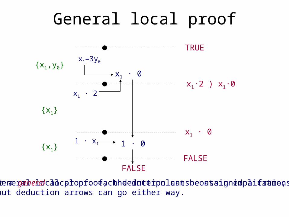
General local proof

x1=3y0

x1 · 2

1 · x1

{x1,y0}

{x1}

{x1}

General local proof: each deduction can be assigned a frame,but deduction arrows can go either way.For a general local proof, the interpolants contain implications.

TRUE

x1·2 ) x1·0

x1 · 0

FALSE

x1 · 0

1 · 0

FALSE

Refinement methods

• Strongest postcondition (SLAM1)• Weakest precondition (Magic,FSoft,Yogi)• Interpolant methods

– Feasible interpolation (BLAST, IMPACT)– Bounded provers (SATABS)– Constraint-based (ARMC)

Local proof

Refinement with SP• The strongest post-condition of w.r.t. progam , written SP(,), is the

strongest such that {} {}.• The SP exactly characterizes the states reachable via .

False

x1=y0

True

y1>x1

x=y;

y++;

[x=y]

x1= y0

y1=y0+1

x1=y1

{False}

{x=y}

{True}

{y=x+1}

x = y

y++

[y·x]

Refinement with SP: Syntactic SP computation:

{} [] { Æ }

{} x := e {9 v [v/x] Æ x = e[v/x]}

{} havoc x {9 x }

This is viewed as symbolic execution,but there is a simpler view.

SP as local proof• Order the variables by their creation in SSA form:

x0 Â y0 Â x1 Â y1 Â

• Refinement with SP corresponds to local deduction with these rules:

x = e

[e/x]x max. in

FALSE unsat.

• We encode havoc specially in the SSA:

havoc x x = iwhere i is a

fresh Skolem constant

Think of the i’s as implicitly existentially quantified

SP example

y0 = 1

x1=y0

y1=y0+1

y1·x1

{x1,y0}

{x1,y0,y1}

{x1,y1}

Ordering of rewrites ensures forward local proof.The (conjunction of) assertions crossing frame boundaryis an interpolant with i’s existentially quantifed.

TRUE

91 (x1=1 Æ y0 = 1)

FALSE

x1 = 1

y1 = 1+1

y1 · 1

1+1·1

FALSE

91 (x1=1 Æ y1 = 1+1)

x1 = y0

y1 = x0 + 1

We can use quantifier elimination if our logic supports it.

Witnessing quantifiers• What happens if we can’t eliminate the quantifiers?

– We can witness them by adding auxiliary variables to the program.

False

True

x=y;

y++;

[x=y]

x1= y0

y1=y0+1

x1=y1

{False}

{True}

x = y

y++

[y · x]

Refinement with SP:

{91 (x=1 Æ y = 1)}

{91 (x=1 Æ y = 1+1)}

havoc y

Predicate abstractioncan’t reproduce this proof!

havoc y1 = yx = y

{x=1 Æ y = 1}

{x=1 Æ y = 1+1}

Will the auxiliary variablesget out of control?

Proof reduction

y0 = 1

x1=y0+1

z1=x1+1

x1·y0

y0 · z1

{x1,y0}

{x1,y0,z1}

{x1,y0,z1}

TRUE

91 (x1=1+1 Æ y0 = 1)

FALSE

x1 = 1+1

z1 = 1+2

1+1·1

FALSE

91 (x1=1 Æ y1 = 1+1 Æ z1=1+1)

• By dropping unneeded inferences, we can weaken the interpolant and eliminate irrelevant predicates.

1 · 1+2x1 · 1

91 (x1=1 Æ y1 = 1+1)

Newton does this to eliminate irrelevant predicates.

Refinement methods

• Strongest postcondition (SLAM1)• Weakest precondition (Magic,FSoft,Yogi)• Interpolant methods

– Feasible interpolation (BLAST, IMPACT)– Bounded provers (SATABS)– Constraint-based (ARMC)

Local proof

Refinement with WP• The weakest (liberal) pre-condition of w.r.t. progam , written WP(,),

is the weakest such that {} {}.• The WP characterizes the states may not reach :.

False

x1=y0

True

y1>x1

x=y;

y++;

[x=y]

x1= y0

y1=y0+1

x1=y1

{False}

{x < y+1}

{True}

{x<y}

x = y

y++

[y·x]

Refinement with WP: Syntactic WP computation:

{}[]{ ) }

{}x := e{[e/x]}

{}havoc x{8 x }

This can also be viewed aslocal proof.

WP as local proof• Order the variables by their creation in SSA form:

x0 Â y0 Â x1 Â y1 Â

• Refinement with WP corresponds to local deduction with these rules:

x = e

[e/x]x min. in

FALSE unsat.

• We encode havoc specially in the SSA:

havoc x x = iwhere i is a

fresh Skolem constant

Think of the i’s as implicitly existentially quantified

WP example

y0 = 1

x1=y0

y1=y0+1

y1·x1

{x1,x0}

{x1,y0,y1}

{x1,y1}

Ordering of rewrites ensures reverse local proof.The negation of assertions crossing frame boundary(with i’s existentially quantified) is an interpolant.

TRUE

FALSE

No need for quantifier elimination in this example.

y0+1 · y0

1+1· 1

FALSE

y0+1 · x1

: y1· x1

: y0+1 · x1

Observations• WP allows proof reductions, just like SP• We are allowed to mix forward and backward rewriting (SP and WP)

– Result is a general local proof, which we can interpolate.– However, forward rewriting may have advantages for Boolean programs,

since it always produces conjunctions.

Abstracting paths• Removing irrelevant assignments and constraints can prevent SP and

WP from introducing irrelevant predicates.

havoc b;c := b;

a := 3c + b;

[a < b];

[c < a]

{True}

{b = 1 Æ c = 1}

{b = 1 Æ c = 1 Æ a = 41}

{41 < 1 Æ c = 1 Æ a = 41}

{False}

1 = b;

Proof using SP...

irrelevant!havoc a;

{b = 1 Æ c = 1 Æ a = 2}

{2 < 1 Æ c = 1 Æ a = 2}

2 = a;

{b = c}

{b = c}

{a < c}

After quantifier elimination...

Abstracting paths very important to keep SP and WP simple

Quantifier divergence• SP and WP introduce quantifiers• Quantifiers can diverge as we consider longer paths through loops

a = 1;b = 0;while (*) { a : = 3a^3 – b; if (a > 0) b = b + a;}assert b >= 0;

Example program:

(Complicated, but irrelevant)

Quantifier divergence

a:= 1;b := 0;

a := 3a3 - b;[a > 0];

b := b + a;

[b < 0]

{True}

{a = 1 Æ b = 0}

{1 > 0 Æ b = 1}

{1 > 0 Æ 2 > 0 Æ b = 1 + 2}

{False}

Proof using SP...

irrelevant!{b = 0}

{b ¸ 1}

{b ¸ 2}

After quantifier elimination...

QE is difficult, but necessary for loops with SP and WP.

a := 3a3 - b;[a > 0];

b := b + a;

irrelevant!

havoc a;[a > 0];

b := b + a;

havoc a;[a > 0];

b := b + a;

Skolem constants diverging!

This predicate is sufficient for PA.

Refinement quality• Refinement with SP and WP is incomplete

– May exists a refinement that proves program but we never find one• These are weak proof systems that tend to yield low-quality proofs• Example program:

x = y = 0;while(*) x++; y++;while(x != 0) x--; y--;assert (y == 0);

{x == y}

invariant:

{y = 0}

{y = 1}

{y = 2}

{y = 1}

{y = 0}

{False}

{True}

{x = y}

{x = y}

{x = y}

{x = y}

{x = y}

{False}

{True}

Execute the loops twice

This simple proof contains invariants

for both loops

• Predicates diverge as we unwind• A practical method must somehow

prevent this kind of divergence!

x = y = 0;

x++; y++;

x++; y++;

[x!=0];x--; y--;

[x!=0];x--; y--;

[x == 0][y != 0]

Refine with SP (and proof reduction)

Same result with WP!

We need refinement methods that can generate simple proofs!

Refinement methods

• Strongest postcondition (SLAM1)• Weakest precondition (Magic,FSoft,Yogi)• Interpolant methods

– Feasible interpolation (BLAST, IMPACT)– Bounded provers (SATABS)– Constraint-based (ARMC)

Local proof

Bounded Provers [SATABS]

• Define a (local) proof system– Can contain whatever proof rules you want

• Define a cost metric for proofs– For example, number of distinct predicates after dropping subscripts

• Exhaustive search for lowest cost proof– May restrict to forward or reverse proofs

x = e

[e/x]x max. in

FALSE unsat.

Allow simple arithmetic rewriting.

Loop example

x0 = 0y0 = 0

x1=x0+1y1=y0+1

TRUE

x0= 0Æ y0 = 0

...

x1=1 Æ y1 = 1x2=x1+1y2=y1+1

...

x1 = 1y1 = 1

x2 = 2y2 = 2

... ...

cost: 2N

x2=2 Æ y2 = 2

x0 = y0

x1 = y0+1

x1 = y1

x2 = y1+1

x2 = y2

TRUE

x0 = y0

...

x1= y1

cost: 2

x2= y2

Lowest cost proof is simpler, avoids divergence.

Lowest-cost proofs• Lowest-cost proof strongly depends on choice of proof rules

– This is a heuristic choice– Rules might include bit vector arithmetic, arrays, etc...– May contain SP or WP (so complete for refuting program paths)

• Search for lowest cost proof may be expensive!– Hope is that lowest-cost proof is short– Require fixed truth value for all atoms (refines restricted case)

• Divergence is still possible when a terminating refinement exists– However, heuristically, will diverge less often than SP or WP.

Refinement completeness• Refinement completeness: if, within the abstraction framework, an

abstraction exists that proves a given program safe, then refinement eventually produces such an abstraction.– Example: predicate abstraction over LRA. If there exists an inductive

invariant proving safety in QFLRA, then the predicate set eventually contains the atomic predicates of such an invariant.

• Some kinds of bounded provers can achieve refinement completeness:– For a stratified language {Li}, when the Li-bounded local proof system is

complete for consequence generation in Li.

– Under certain conditions, for bounded local saturation provers, including first-order superposition calculus provers.

So we know that local provers can avoid divergence.The key question is whether the cost of finding thebest proofs is justified in practice.

Refinement methods

• Strongest postcondition (SLAM1)• Weakest precondition (Magic,FSoft,Yogi)• Interpolant methods

– Feasible interpolation (BLAST, IMPACT)– Bounded provers (SATABS)– Constraint-based (ARMC)

Local proof

Constraint-based interpolants• Farkas’ lemma: If a system of linear inequalities is UNSAT, there is a

refutation proof by summing the inequalities with non-neg. coefficients.• Farkas’ lemma proofs are local proofs!

x0 · 00 · y0

x1·x0+1z1·x1-1

y0+1·y1

y1+1·x1

1 (y0+1·y1)1 (y1+1·x1)

1 (x0 · 0)1 (0 · y0)

x0 · y0

1 (x1·x0+1)0 (z1·x1-1)

x1 · y0

1 · 0

Intermediate sums arethe interpolants!

x0 · y0

x1 · y0

1 · 0

0 · 0

Coefficients can be foundby solving an LP.

Interpolants can becontrolled with additionalconstraints.

.

Refinement methods

• Strongest postcondition (SLAM1)• Weakest precondition (Magic,FSoft,Yogi)• Interpolant methods

– Feasible interpolation (BLAST, IMPACT)– Bounded provers (SATABS)– Constraint-based (ARMC)

Local proof

Interpolation of non-local proofs• In some logics, we can translate a non-local proof into interpolants.

– propositional logic– linear arithmetic (integer or real)– equality, function symbols, arrays

• In most case, QF formulas yield QF interpolants, solvingthe quantifier divergence problem.– use of the array theory is limited

• This is an advantage, since searching for a non-local proof is easier– can be accomplished with standard decision procedures

Non-local to local• We can think of interpolation as translating a non-local proof into a local

proof.

x0 · y0

x1·x0-1

x2· x1-1y0·x2

x0 · y0

x1 · y0-1

0 · -2

0 · 0

x2 · x0-2

x2 · y0-2

0 · -2

Non-local!

Interpolation re-orders thesum to make the proof local.

x1· y0-1

x2· y0-2

0·-2

• Interpolation makes proof search easier, but can substantially reduce the cost of the proof, possibly leading to divergence,

Refinement methods• Strongest postcondition (SLAM1)• Weakest precondition (Magic,FSoft,Yogi)• Interpolant methods

– Feasible interpolation (BLAST, IMPACT)– Bounded provers (SATABS)– Constraint-based (ARMC)

Local proof

These methods can be viewed as different strategies to search fora local proof, trading off the cost of the search and the quality ofthe interpolants.

Basic Framework• Abstraction and refinement are proof systems

– spaces of possible proofs that we search

Abstractor

Refiner

General proof system

Incomplete

Specialized proof system

Complete

prog.

pf. special case cex.

pf. of special case

Degree of specialization can strongly affect refinement quality

Predicate abstraction• In predicate abstraction, we typically build a graph in which the vertices

are labeled with minterms over P (abstract states).• The proof is complete when it folds into a Hoare logic proof of C.• An unprovable path looks like this:

1 2 3 4 5

1 2 3 4 5

no individual transition refutable

• To refine, translate to restricted program path:

[1];1 [

2];2 [

3];3 [

4];4 [

5];5

Any proof of this restricted path rules out the original, but...

Overspecialization• Restricting paths can affect the quality of the refinement.

x=0

x++

x++

x++

[x < 0]

[x=0]

[x=0]

[x=1]

[x=2]

[x 0,1,2]

Restricted path, from PA({x=0,x=1,x=2})

Lowest-cost proof leads to divergence!

Lowest-cost proof without restriction.

{x=3}

{False}

{True}

{0 · x}

{0 · x}

{0 · x}

{False}

Restricting paths can make the refiner’sjob easier. However, it also skews theproof cost metric. This can cause therefiner to miss globally optimal proofs,leading to divergence.

Synergy algorithm• The Synergy algorithm produces a very local refinement by strongly

restricting the refinement path.

1 2 3 4 5

1 2 3 4 5

Shortest infeasible prefix

Restrict to concrete states.

{}Refinement only here!4

3

3Æ:

Æ

...splits just one state!

• Synergy produces small incremental refinements at low cost.• However, extreme specialization can reduce quality of refinements

leading to divergence for loops.

Summary• Abstraction and refinement can be thought of as two proof systems:

– Abstractor is general, but incomplete– Refiner is specialized, but complete.

• Abstraction is path-reductive is, when it fails, it fails for one path.– Refiner generates path proof– Abstractor replicates proof

• Existing refiners can be viewed as local proof systems– Quality of proof depends on proof system, search strategy– Low refinement quality leads to divergence– Different refines represent different cost/quality trade-offs

• Abstractors vary in the refinement proof goals generated– Specialization reduces cost, but also refinement quality.– In general, the more the refiner sees, the better the refinement

Three ideas to take away• An abstraction is a restricted deduction system.• A proof decomposition divides a proof into shallow lemmas, where

shallow means "can be proved in a simple abstraction"• Relevant abstractions are discovered by generalizing from particular

cases.

By applying these three ideas, we can increase thedegree of automation in proofs of complex systems.