abstract veeramani, arun shankar. a transformative tool
TRANSCRIPT

ABSTRACT
VEERAMANI, ARUN SHANKAR. A Transformative Tool for Minimally Invasive Procedures: Design, Modeling and Real-Time Control of a Polycrystalline Shape Memory Alloy Actuated Robotic Catheter. (Under the direction of Dr. Gregory D. Buckner).
Cardiac catheterization is rapidly transforming the diagnosis and treatment of
cardiovascular disease. However, the use of catheters is limited to procedures
where the target anatomy can be easily accessed via natural vasculature.
Robotically controlled catheters have the potential to provide greater access and
more precise interaction with internal anatomies. This dissertation presents the
development of a shape memory alloy (SMA) actuated robotic catheter: from
electromechanical design to the development of novel modeling and control
approaches.
The robotic catheter is fabricated using conventional manufacturing and rapid
prototyping. To analyze the transient characteristics of the catheter, a dynamic
model is developed. Its bending mechanics are derived using a circular arc model
and are experimentally validated. The effects of outer sleeve thickness on heat
transfer and transient response characteristics are studied. SMA actuation is
described using the Seelecke-Muller-Achenbach model for single-crystal SMA with
experimentally determined parameters. Joule heating is used to generate tip
deflections, which are measured in real-time using a dual-camera imaging system.
The dynamic characteristics of this active catheter system are simulated and
validated experimentally.
The direct extension of the Seelecke-Muller-Achenbach model to a catheter with
multiple SMA tendons proves difficult because of the computational cost and
inherent inaccuracies of single-crystal modeling assumptions. Moreover, the
requisite variable-step solvers are not suitable to real-time control. To facilitate more

accurate modeling and effective real-time control of an SMA catheter with multiple
tendons, a new modeling technique based on Hysteretic Recurrent Neural Networks
(HRNNs) is proposed. Its efficacy is demonstrated experimentally for two- and three-
phase hysteretic systems. The HRNN is shown to accurately capture the
polycrystalline stress-strain characteristics of SMA tendons at different
temperatures.
A robotic catheter system consisting of four SMA tendons is then decoupled into
two planar bending systems, each containing a pair of antagonistic SMA tendons.
An HRNN model is developed directly from experimental output measurements, and
is used to develop a feed-forward controller.

A Transformative Tool for Minimally Invasive Procedures:
Design, Modeling and Real-Time Control of a Polycrystalline Shape Memory Alloy
Actuated Robotic Catheter
by Arun Shankar Veeramani
A dissertation submitted to the Graduate Faculty of North Carolina State University
in partial fulfillment of the requirements for the Degree of
Doctor of Philosophy
Mechanical Engineering
Raleigh, North Carolina
2009
APPROVED BY:
_________________________________ _________________________________ Stefan Seelecke M. K. Ramasubramanian _________________________________ _________________________________ Denis R. Cormier Gregory D. Buckner Chair of Advisory Committee

ii
Dedication
To Appa and Amma

iii
Biography
Arun Veeramani was born in Chengalpet, Tamil Nadu, India. He received the
Bachelor of Engineering degree in Electronics and Instrumentation from the
University of Madras (Tamil Nadu, India) in 1999. He started graduate studies at
North Carolina State University in 2003, where he received the Master of Science
degree in Electrical Engineering in 2004. In 2005, he began doctoral studies in
Mechanical Engineering under the direction of Dr. Gregory D. Buckner.

iv
Acknowledgements
I owe my sincerest gratitude to Dr. Gregory Buckner for his constant
encouragement, support and timely guidance throughout the course of this doctoral
research. He has afforded me immense freedom to pursue my scientific interests
and has taken personal interest in ensuring my success in this research. This
research experience has transformed me as a person and I thank him for this
opportunity.
I thank my doctoral committee members, Dr. Stefan Seelecke, Dr. Denis Cormier
and Dr. M. K. Ramasubramanian for their time, encouragement and advice.
I thank all the current and past members of the Electromechanics Research
Laboratory: John Crews, Brian Owen, Shaphan Jernigan, Andy Richards and
Pradeep Pandurangan for their help with this research. I’m especially thankful to
John Crews and Brian Owen for their contributions.
I thank all my friends: Chitti, Krish, Dinesh, Jaggu, Nikhil, Kumar, Prem,
Shrikanth, Deepak, Praveen, Remya and so many others who have been great
support and made these years in graduate school memorable.
I owe all that I am today to my family, especially my parents, brother and
grandparents. Thanks for your love and encouragement, for believing in me and
supporting me in all my endeavors including this one. I thank Maha for being
supportive and understanding during the tough times. I thank Mama and Chithi for
their support and encouragement through these years.

v
Table of Contents
List of Figures ....................................................................................................... viii
List of Tables ......................................................................................................... xvi
Chapter 1. Introduction ....................................................................................... 1
1.1 Minimally invasive surgery ..................................................................... 1
1.2 Cardiac catheters ................................................................................... 2
1.3 Common commercial passive catheters ................................................. 6
1.4 Steerable catheters ................................................................................ 8
1.5 Robotic catheters ................................................................................. 10
1.6 Research objectives ............................................................................. 13
1.7 Outline of dissertation ........................................................................... 15
Chapter 2. Design of SMA Actuated Robotic Catheter ................................... 17
2.1 Single-segment catheter design ........................................................... 17
2.2 Single-segment catheter modeling ....................................................... 23
2.3 Catheter bending model ....................................................................... 25
2.4 SMA constitutive model ........................................................................ 31
2.5 Experimental determination of SMA model parameters ....................... 36
2.6 Heat transfer model .............................................................................. 41
2.7 Complete single-segment catheter model ............................................ 47
2.7.1 Experimental setup for measuring catheter tip response ............................. 48
2.7.2 Catheter actuation experiments ................................................................... 49
2.8 Extension of bending mechanics to four-tendon catheter ..................... 56
2.8.1 Decoupling catheter dynamics in orthogonal planes .................................. 58

vi
2.8.2 Occurrence of slack in the PCB system ....................................................... 63
Chapter 3. Hysteretic Recurrent Neural Networks.......................................... 65
3.1 Introduction .......................................................................................... 65
3.2 Hysteretic Recurrent Neural Network ................................................... 69
3.3 Modeling magnetic hysteresis .............................................................. 73
3.4 Modeling two-phase transformations in SMA ....................................... 80
3.5 Modeling three-phase transformations in SMA .................................... 86
3.5.1 Stress-based HRNN .................................................................................... 88
3.5.2 Strain-based HRNN ..................................................................................... 94
3.5.3 Validation of three-phase HRNN .................................................................. 96
3.6 Modeling three-phase transformations in SMA using output
measurements ................................................................................... 100
3.7 Modeling schemes for a SMA-spring system ..................................... 103
3.7.1 Explicit modeling scheme .......................................................................... 104
3.7.2 Implicit modeling scheme ........................................................................... 120
3.8 Modeling planar catheter actuation with antagonistic SMA tendons .. 125
3.8.1 Parallel combination of SCSMA elements ................................................. 125
3.8.2 Series combination of SCSMA elements ................................................... 132
3.8.3 Training HRNNs for the PCB system ......................................................... 137
Chapter 4. Control of the Robotic Catheter ................................................... 142
4.1 Introduction ........................................................................................ 142
4.2 Control system setup .......................................................................... 143
4.3 HRNN based control of PCB system .................................................. 146
4.4 Simulated control results .................................................................... 151
4.4.1 Step response ............................................................................................ 151
4.4.2 Sinusoidal tracking response ..................................................................... 153

vii
4.4.3 Comparison to PID control ......................................................................... 154
4.5 Control of a single-segment robotic catheter ...................................... 159
4.5.1 Regulation control ...................................................................................... 159
4.5.2 Tracking control ......................................................................................... 161
Chapter 5. Conclusions .................................................................................. 165
5.1 Future work ........................................................................................ 167
References ………… ............................................................................................ 169

viii
List of Figures
Figure 1.1 A commercial lead placement catheter from Medtronic [70] ..................... 3
Figure 1.2 (a) Ablation being performed inside the atrium [72] and (b) Ablation
catheter inserted through the femoral artery [73] ................................... 4
Figure 1.3 Placing a pacing lead on the epicardial surface [74] ................................. 5
Figure 1.4 Deployment of a Foley catheter [75] ......................................................... 6
Figure 1.5 Branching of the vasculature .................................................................... 8
Figure 1.6 Catheters with (a) single direction and (b) bi-directional steering
capabilities ............................................................................................. 9
Figure 2.1 Candidate robotic catheter architectures: (a) MEMS based design and (b)
design featuring articulated joints ........................................................ 19
Figure 2.2 Preliminary design concepts based on monolithic beam substructures .. 20
Figure 2.3 Final robotic catheter architecture ........................................................... 20
Figure 2.4 PWM control circuit for electrical activation of SMA tendons .................. 23
Figure 2.5 Open loop control schematic for the robotic catheter .............................. 23
Figure 2.6 Simplified catheter system for modeling and analysis ............................ 24
Figure 2.7 Block diagram of active catheter model .................................................. 24
Figure 2.8 Free body diagrams of (a) central tube and (b) SMA tendon in initial
(straight) state ...................................................................................... 25
Figure 2.9 Free body diagram of (a) central tube after a small deflection θ; (b)
exaggerated drawing of the (a); (c) exaggerated drawing of segment
OA after a small deflection θ ................................................................ 27
Figure 2.10 Time-lapsed photography of the catheter bending as a function of
applied current, with circular arc references ........................................ 31

ix
Figure 2.11 Phase transformations in shape memory allows: superelastic and shape
memory effects .................................................................................... 32
Figure 2.12 Setup for dynamic, temperature-controlled tensile testing of SMA
specimens ............................................................................................ 37
Figure 2.13 Stress-strain curves for nitinol specimen vs. temperature: a) loading and
b) unloading ......................................................................................... 38
Figure 2.14 Variation in bend angle vs. tendon-neutral axis distance at 95 deg C .. 40
Figure 2.15 Temperature profile in SMA tendon, outer sleeve, and ambient air ...... 41
Figure 2.16 Setup for investigating effects of outer sleeve thickness ....................... 45
Figure 2.17 SMA displacement responses vs. sleeve thickness .............................. 46
Figure 2.18 Two-camera measurement system for tracking 3-D position of catheter
tip ......................................................................................................... 49
Figure 2.19 Experimental catheter bending responses (a) and SMA temperature
responses (b) for 0.0043 Hz input current pulses (c) ........................... 50
Figure 2.20 Simplified cross-section of the catheter with SMA tendon placed (a)
concentrically and (b) eccentrically inside the sleeve .......................... 51
Figure 2.21 Temperature response for 0.00434Hz current pulse: (a) experimental,
(b) simulated using heat transfer model (15-18), (c) simulated using
identified model (2.22) ......................................................................... 53
Figure 2.22 Temperature response for 0.1 Hz current pulses: (a) experimental, (b)
simulated using identified model (2.22) ............................................... 54
Figure 2.23 Experimental vs. simulated active catheter bending responses: (a)
measured response to 0.0043Hz current pulse, (b) simulated response
to 0.0043Hz current pulse, (c) measured response to 0.1Hz current
pulse, (d) simulated response to 0.1Hz current pulse .......................... 55

x
Figure 2.24 Catheter kinematics .............................................................................. 58
Figure 2.25 PCB system in xz plane ....................................................................... 60
Figure 2.26 Slack development in SMA tendons: (a) neutral position, (b) xz+ tendon
actuated, and (c) appearance of slack in the xz− tendon .................... 64
Figure 3.1 Illustration of a Preisach operator ........................................................... 66
Figure 3.2 Hysteretic kernel consisting of conjoined sigmoid activation functions ... 69
Figure 3.3 Hysteretic Recurrent Neural Network (HRNN) architecture .................... 71
Figure 3.4 Schematic of the experimental setup for measuring magnetic hysteresis
............................................................................................................. 74
Figure 3.5 Photograph of the experimental setup for measuring magnetic hysteresis
............................................................................................................. 74
Figure 3.6 Experimental input (a) and output (b) data acquired from the setup ....... 75
Figure 3.7 HRNN training results: (a) cost functions during training; (b) comparison
of training data vs. HRNN predictions for ascending transitions; (c)
comparison of training data vs. HRNN predictions for descending
transitions ............................................................................................ 76
Figure 3.8 RBFN training results: (a) comparison of training data vs. network
predictions for ascending transitions; (b) comparison of normalized
training data vs. network predictions for descending transitions .......... 77
Figure 3.9 HRNN and RBFN test results: (a) test input data; (b) test output data; (c)
comparison of test data vs. network predictions; (d) comparison of test
error for both networks ......................................................................... 79
Figure 3.10 Schematic of experimental setup for measuring SMA hysteresis ......... 81
Figure 3.11 Photograph of experimental setup for measuring SMA hysteresis ....... 81

xi
Figure 3.12 Experimental training data acquired from the SMA test rig: (a) input
current, (b) SMA surface temperature, (c) SMA displacement ............. 82
Figure 3.13 Experimental validation data acquired from the SMA test rig: (a) input
current, (b) SMA surface temperature, (c) SMA displacement ............. 83
Figure 3.14 HRNN training results: (a) comparison of training data vs. HRNN
predictions for ascending transitions; (b) comparison of training data vs.
HRNN predictions for descending transitions; (c) comparison of
validation data vs. HRNN predictions .................................................. 85
Figure 3.15 Weights of the neurons for the forward transition values (a); Weights of
the neurons for the reverse transition values (b) .................................. 86
Figure 3.16 Representation of polycrystalline SMA specimen as a parallel (a) or
series (b) combination of SCSMA elements ........................................ 88
Figure 3.17 Three-phase, stress-based HRNN neuron ............................................ 91
Figure 3.18 Stress-strain characteristics simulated using a single stress-based
neuron at different temperatures .......................................................... 93
Figure 3.19 Three-phase HRNN architecture using stress-based neurons .............. 94
Figure 3.20 Three-phase, strain-based HRNN neuron ........................................... 95
Figure 3.21 Three-phase HRNN architecture using strain-based neurons .............. 96
Figure 3.22 Comparison of training data and HRNN predictions for: (a) 24 °C; (b) 45
°C; (c) 75 °C; (d) 95 °C ........................................................................ 98
Figure 3.23 Comparison of validation data and HRNN predictions for: (a) 24 °C; (b)
45 °C; (c) 75 °C; (d) 95 °C ................................................................... 99
Figure 3.24 Comparison of test data and HRNN prediction for: (a) 35 °C; (b) 55 °C;
(c) 65 °C; (d) 85 °C ............................................................................ 100
Figure 3.25 Series combination of SCSMA elements ............................................ 101

xii
Figure 3.26 Three-phase HRNN training results: (a) comparison of training data vs.
HRNN predictions for ascending transitions; (b) comparison of training
data vs. HRNN predictions for descending transitions ....................... 103
Figure 3.27 Single-input, single-output SMA-spring system .................................. 104
Figure 3.28 Explicit modeling scheme for SMA-spring system .............................. 104
Figure 3.29 (a) Stress-strain operating point iB at 1k ; (b) Strain-temperature
relationship at 1k ................................................................................ 108
Figure 3.30 (a) Stress-strain operating point 4( )oB k ; (b) Strain-temperature
relationship at 4k ............................................................................... 111
Figure 3.31 (a) Stress-strain operating point 5( )oB k ; (b) Strain-temperature
relationship at 5k ............................................................................... 112
Figure 3.32 (a) Stress-strain operating point ( )6oB k ; (b) Strain-temperature
relationship at 6k ............................................................................... 113
Figure 3.33 Time evolution of a stable simulation: (a) stress-strain plot and (b)
actuation output ................................................................................. 114
Figure 3.34 MATLAB simulation of explicit modeling scheme: (a) Stress-strain plot
and (b) actuation output ..................................................................... 114
Figure 3.35 (a) Stress-strain operating point 4( )oB k ; (b) Strain-temperature
relationship at 4k ............................................................................... 116
Figure 3.36 (a) Stress-strain operating point 5( )oB k ; (b) Strain-temperature
relationship at 5k ............................................................................... 117

xiii
Figure 3.37 (a) Stress-strain operating point 6( )oB k ; (b) Strain-temperature
relationship at 6k ............................................................................... 118
Figure 3.38 Time evolution of an unstable simulation: (a) stress-strain plot and (b)
actuation output ................................................................................. 119
Figure 3.39 Stress-strain plot (a) and actuation output (b) of an unstable simulation
in MATLAB ......................................................................................... 119
Figure 3.40 Block diagram for implicit modeling scheme ....................................... 121
Figure 3.41 (a) Simulated actuation response of SMA actuator and (b) simulated
strain-strain behavior of two of the neurons in the HRNN for
temperature input (c) ......................................................................... 124
Figure 3.42. (a) SMA tendons represented as parallel combination of SCSMA
elements and (b) Equivalent representation in terms of spring and
parallel SCSMA elements .................................................................. 126
Figure 3.43 Actuation of PCB system: (a) tendon strains (b) temperature applied to
individual tendons .............................................................................. 131
Figure 3.44. SMA tendons represented as a series combination of SCSMA elements
........................................................................................................... 132
Figure 3.45 Experimental training data obtained from the PCB system: (a) input and
(b) output ........................................................................................... 138
Figure 3.46 Experimental test data obtained from the PCB system: (a) input and (b)
output ................................................................................................. 138
Figure 3.47 Comparison of experimental training data and HRNN predictions ...... 140
Figure 3.48 Comparison of experimental test data with HRNN predictions ........... 141
Figure 4.1 Decoupled control architecture for single-segment catheter ................. 145
Figure 4.2 Schematic of the single-segment catheter control system .................... 146

xiv
Figure 4.3 HRNN based feed-forward controller for a PCB system ....................... 147
Figure 4.4 Algorithm for computing the pseudoinverse .......................................... 149
Figure 4.5 Simulated step response of HRNN-based feed-forward controller ....... 152
Figure 4.6 Step response results: (a) simulated PWM input to each tendon, (b)
estimated tendon temperatures ......................................................... 152
Figure 4.7 Simulated sinusoidal tracking response of HRNN-based feed-forward
controller ............................................................................................ 153
Figure 4.8 Sinusoidal tracking results: (a) simulated PWM inputs to each tendon, (b)
estimated tendon temperatures ......................................................... 154
Figure 4.9 PID controller architecture .................................................................... 154
Figure 4.10 Simulated step response comparisons: output responses of HRNN-
based feed-forward controller and PID controller ............................... 155
Figure 4.11 Step response comparisons: estimated tendon temperatures for HRNN-
based feed-forward controller and PID controller: (a) xz+ tendon and
(b) xz− tendon ................................................................................... 156
Figure 4.12 Step response comparisons: simulated PWM inputs to each tendon for
HRNN-based feed-forward controller and PID controller: (a) xz+ tendon
and (b) xz− tendon ............................................................................ 156
Figure 4.13 Simulated sinusoidal tracking comparisons: output responses of HRNN-
based feed-forward controller and PID controller ............................... 157
Figure 4.14 Sinusoidal tracking comparisons: estimated tendon temperatures for
HRNN-based feed-forward controller and PID controller: (a) xz+ tendon
and (b) xz− tendon ............................................................................ 158

xv
Figure 4.15 Sinusoidal tracking comparisons: simulated PWM inputs to each tendon
for HRNN-based feed-forward controller and PID controller: (a) xz+tendon and (b) xz− tendon ................................................................ 158
Figure 4.16 Experimental step response comparisons: output responses of PI and
PID controllers: (a) Bending angle, (b) Orientation angle................... 160
Figure 4.17 Experimental step response comparisons: PWM inputs to each tendon
for PI and PID controller: (a) xz plane and (b) yz plane ....................... 160
Figure 4.18 Three-dimensional representation of the circular trajectory tracking ... 162
Figure 4.19 Experimental tracking of a circular trajectory: output responses of PI and
PID controllers: (a) Bending angle, (b) Orientation angle................... 163
Figure 4.20 Experimental tracking of a circular trajectory: PWM magntidues: (a) xz
plane, (b) yz plane .............................................................................. 163

xvi
List of Tables
Table 2.1 Physical constants and parameters of the active catheter prototype .. 47
Table 4.1 Controller parameters ....................................................................... 151

1
Chapter 1. Introduction
1.1 Minimally invasive surgery
Over the past two decades, the surgical treatment of a variety of diseases has
transitioned from highly invasive and traumatic procedures to the newly emerging
paradigm of minimally invasive procedures. Instead of making large incisions to gain
access to internal anatomy, minimally invasive procedures make use of small
incisions (ports) that are typically 10-15mm in length. Laparoscopic instruments,
endoscopes and other percutaneous tools are deployed through these incisions,
enabling the physician to operate effectively inside the body. Tasks such as cutting,
cauterizing and suturing tissue are performed using different types of end effectors
mounted at the distal end of laparoscopic instruments. Visualization of internal
anatomy is provided by endoscopes and further aided by fluoroscopy.
Minimally invasive procedures have been widely adopted by a variety of surgical
specialties including cardiothoracic, vascular, neurological, urological and pediatric
surgery. The benefits of minimally invasive procedures include:
1) Shorter hospital stays
2) Cosmetically superior outcomes
3) Reduced post-operative trauma and pain
These benefits have the potential to reduce overall healthcare costs and improve
post-operative quality of life.
Despite two decades of development, there remain significant opportunities for
improvement in minimally invasive surgery through the development of new surgical
instruments. Robotic catheter technologies have the potential to provide superior
access, visualization and maneuverability inside the body than conventional rigid

2
laparoscopic tools. Conventionally, catheters are used to perform tasks such as
delivering or drawing fluids, measuring flow rates and pressures and deploying
prosthetic devices. However, if equipped with robotic control capabilities and multiple
degrees of freedom, they have the potential to transform a range of surgical
procedures into minimally invasive procedures.
1.2 Cardiac catheters
Catheters are essentially thin flexible tubes introduced percutaneously, generally
into major blood vessels, to perform a variety of interventions inside the body. The
use of catheters dates back over 2000 years, when simple rigid metal or wooden
tubes were used to empty the bladder. Modern-day catheters have become
increasingly sophisticated, and have been adapted for use in a number of different
pathologies. The most common applications are in the areas of urology, cardiology
and neurology.
Cardiac catheterization is rapidly transforming the diagnosis and treatment of a
number of cardiovascular diseases. Although not considered clinically safe until the
1940s, the use of cardiac catheters is now standard practice. The American Heart
Association estimates that in 2004 over 1.4 million diagnostic cardiac
catheterizations were performed in the United States, as well as 1.25 million
angioplasties and 615,000 stent placement procedures [1]. These numbers
constitute a 334 percent increase in cardiac catheterizations from 1979-2003.
Specific catheterization procedures include angioplasty and stent placement within
the coronary arteries, placement of pacing leads in the heart chambers and coronary
sinus, ventricular biopsies, atrial ablation, and cardiac mapping. Figure 1.1 shows a
typical commercial catheter used for the placement of pacing leads inside the heart.

3
Figure 1.1 A commercial lead placement catheter from Medtronic [70]
Owing to the importance of cardiac catheters, this research aims to develop a
robotic catheter whose design is guided by two potential applications in cardiac
surgery: cardiac ablation and epicardial lead placement. Cardiac ablation (Figure
1.2a) is a procedure used to treat atrial fibrillation which involves the creation of
incisions or lesions in the atrial tissue to modify the conduction of electrical signals.
Catheter-based ablation starts with the percutaneous insertion of the catheter into a
major blood vessel leading to the heart (Figure 1.2b). Subsequent navigation
through the vessel and inside the heart is achieved by manual steering of the
catheter tip by the physician. After directing the tip to the region of interest on the
endocardial surface, the physician manipulates the tip to create atrial lesions in a
point-by-point method. Lesions are created by applying ablative radiofrequency (RF)
energy at each location for 15-45 second durations. During this time, proper
catheter/tissue contact must be maintained to create effective lesion sets that must
be both transmural (reaching through the depth of the tissue) and continuous.

4
(a) (b) Figure 1.2 (a) Ablation being performed inside the atrium [72] and (b) Ablation catheter
inserted through the femoral artery [73]
Cardiac resynchronization therapy (CRT) (Figure 1.3) is an important treatment
for heart failure patients with cardiac rhythm conduction problems. Successful CRT
involves accurate deployment of pacing leads inside the right atrium (RA) and right
ventricle (RV) and in the Left Ventricle (LV). Although placing leads in RV and RA
can be done efficiently with commercial catheters, placement of the LV lead may not
be straightforward. The most popular approach is placing the LV lead venously
(percutaneously) via the coronary sinus (CS). However, the CS approach often
suffers from shortcomings such as lack of access to optimal sites and long
procedure times that are associated with large exposures to radiation for patients
and physicians. Further, cannulation of the CS is a challenging task considering the
limited steering capabilities of conventional catheters. Epicardial pacing of the LV for
CRT stands as a solution to many of the problems associated with placement of
leads via the CS, as recent advances in epicardial lead design have made them as
reliable as their endocardial counterparts [4,5]. In practice, epicardial pacing has

5
demonstrated the following advantages over placement via the CS: 1) reduced
procedure times, 2) a lower percentage of patients with increased pacing thresholds,
3) fewer complications, 4) more accurate lead placement, 5) less exposure to
radiation, and 6) more flexibility in lead placement [6,7,8,9]. Despite its documented
benefits, epicardial pacing has not been widely adopted because it is more invasive,
requiring open access to the chest cavity via mini-thoracotomy, thoracoscopy, or
median sternotomy. However, a minimally invasive approach to this procedure is
possible if the pacing leads are deployed through subxiphoidal port onto the
epicardial surface using a catheter. But the current catheter technologies are not
suitable for such a procedure as they cannot be maneuvered accurately in open
spaces.
Figure 1.3 Placing a pacing lead on the epicardial surface [74]

6
1.3 Common commercial passive catheters
The typical commercial catheter consists of a passive flexible tube (1.5-8 mm
OD) made of silicone or plastic which is manually advanced into a major vessel. Its
direction of travel is determined by the vessel itself and there is nearly no control of
the tip heading or location. A common example is the Foley catheter used to drain
urine from the bladder. It is manually advanced though the urethra until its tip is in
the bladder, where it is retained using an inflatable balloon at the catheter’s tip
(Figure 1.4).
Figure 1.4 Deployment of a Foley catheter [75]
Because passive catheters lack structural stiffness, some are inserted into
vasculature with the assistance of a guidewire. In these cases, the guidewire
(typically a thin and stiff stainless steel wire, 0.25-1.00 mm in diameter) is first
threaded though the target vessel. The catheter then slides over the guidewire,
enabling it to easily navigate the vessel.
The design of guidewire catheters is based on the following criteria [69]:

7
1) Pushability: This property relates to the ease with which the catheter can be
advanced or pushed into the vessel. Pushability depends on the axial stiffness of
the catheter: higher stiffness makes the catheter easier to push into the vessel
without buckling.
2) Torqueability: This property refers to the ease with which the catheter can be
rotated within the vessel. Sometimes it is necessary to rotate the tip of the
catheter in order to orient it in the desired direction. In such cases the catheter
must be able to transmit a twisting moment from the handle to its tip. This
property is directly related to the torsional stiffness of the catheter.
3) Trackability: This property relates to the ease with which a catheter can navigate
tortuous paths. The factors which determine a catheter’s trackability are its
friction with the surrounding tissue and its flexibility.
Although standard passive catheters and their associated design criteria are
sufficient for routine procedures, they are frequently inadequate for more complex
procedures. A primary limitation is the lack of steerability of the catheter tip when it
encounters a branching of the vasculature as depicted in Figure 1.5.

8
Figure 1.5 Branching of the vasculature
The difficulties in guiding the catheter into the appropriate branch are apparent,
especially when the vessel sizes are relatively small. This is particularly relevant to
cardiac procedures such as ablation, where series of branches need to be
navigated. This issue is overcome to an extent through the use of guidewires, but
not in cases where the path is highly tortuous. Such catheters are also impossible to
use in procedures requiring navigation through open spaces inside the body, such
as epicardial lead placement. This is because these catheters depend heavily on the
surrounding vasculature for guidance.
1.4 Steerable catheters
For the reasons cited above, more complex procedures require the use of
catheters with some degree of tip steerability. Steerable catheters usually provide
this feature in a single bending direction, and are typically actuated using a pull-wire
attached to the tip (Figure 1.6a). The catheter’s distal end (tip) is usually constructed
of a soft material, whereas the catheter body is made of stiffer materials. The pull-
wire is attached to a mechanical lever mechanism at the proximal end (handle);

9
pulling this lever results in local bending of the distal end owing to its lower stiffness.
The physician must rotate the catheter’s handle in order to change the direction of
bending. This relates to the torqueability property of the catheter described earlier. A
common design enhancement involves the incorporation of a second pull-wire to
enable bidirectional bending (Figure 1.6b). Such designs can be extended to include
four pull-wires to enable ‘four-way’ steering.
Figure 1.6 Catheters with (a) single direction and (b) bi-directional steering capabilities
Although most commercial steerable catheters feature pull-wires, there are
shortcomings to this design:
1) Manual actuation: the need for manual manipulation of levers or knobs on the
catheter handle. The physician needs to be highly skilled in order to use such
catheters effectively, a problem that is further exacerbated when multiple levers are

10
used to provide bending in multiple directions. Effective manipulation of the catheter
in open spaces inside the body is nearly impossible due to the absence of
vasculature guidance.
2) Limited degrees of freedom (DOF): most steerable catheters can bend in a
single direction or plane only. Additional DOF come at the expense of increasing the
catheter diameter, which is not desirable.
1.5 Robotic catheters
The shortcomings of conventional steerable catheters described in the previous
section can be overcome by robotic control, which has the potential to improve
steerability, accuracy, precision and ease of use. Such capabilities are extremely
important in procedures such as atrial ablation and epicardial lead placement.
Consequently, robotic catheters have the potential to reduce the duration of these
procedures and improve patient outcomes. Since fluoroscopy is an integral part of
these procedures, shorter procedure times have the added advantage of reduced
exposure to radiation for both the physician and patient.
Realizing the potential benefits of robotic catheterization, two commercial robotic
catheter technologies are currently available. These include the Sensei Robotic
Catheter System [10] (Hansen Medical, Mountain View, CA) and the NIOBE II
Remote Magnetic System [11]. The Sensei Robotic Catheter System is a remotely
operated catheter which allows 3D tip control. This system still uses pull-wires to
control the distal end, but wires are manipulated by servomotors stationed above the
patient. Catheter insertion and withdrawal are also controlled by servomechanisms
outside the patient. The NIOBE II Remote Magnetic System boasts a magnetically
guided catheter tip married to an electroanatomical mapping system. Here, the tip of
a specially designed catheter contains a small magnet which is manipulated by
magnetic fields created by two large and articulating external permanent magnets

11
stationed on opposite sides of the patient. Although these robotic systems are novel
and are currently under clinical use, they are prohibitively expensive. Both systems
require dedicated space in operating rooms or catheterization labs, and both lack the
ability to vary the number of DOF in each catheter.
Apart from these commercial technologies, there has been extensive research in
academic institutions towards developing robotic catheters, cannulas and probes.
Many of these devices use servo-actuated pull-wires as described previously. The
snake-like units described in [13] use multiple ‘backbones’ instead of a single
backbone. These additional backbones provide structural stiffness and actuation
redundancy while functioning as push-pull wires. However, this design suffers from
the same drawbacks as the Sensei Robotic Catheter System because the
underlying principle of operation is similar. Another pull-wire prototype under
development is the Articulated Robotic Medical probe (ARM) [14]. This is a 12 mm
diameter robotic probe is designed to perform procedures through the subxiphoid
space, including epicardial ablation and placement of epicardial pacing leads. Its
novelty lies in the fact that the design can easily be extended to large number of
DOF. The deployment approach involves iteratively ‘freezing’ the shape of the probe
in space and making directional adjustments only to the tip, thus creating a snake
like path in space. However, this method of actuation is not suitable for real-time
manipulation of the probe body through space. Also, the size of the probe is
prohibitively large (12 mm diameter) to be used for intravascular procedures.
Other research has explored alternatives to pull-wires for actuation. One
interesting research prototype is an “active cannula” developed by Webster, et al.
[15]. This device consists of concentric tubes with preset curvatures. Rotation and
translation of individual tubes with respect to each other enables steering of the
cannula in different directions. The actuation of individual tubes is done externally,
making the device bulky. Also, the addition of DOF comes at the expense of

12
increasing the diameter of the device since the tubes need to be placed
concentrically. Electromechanically actuated earthworm-like devices have also been
also been explored [16] to serve as self-propelled endoscopes inside the colon
(colonoscopes). However, these devices and associated mechanisms are too large
to be used inside blood vessels. A survey of such devices can be found in [17].
Utilizing “smart materials” for actuation offer tremendous potential benefits to
robotic catheterization: compact, highly articulated and low-cost robotic catheters
significantly more advanced than current technologies. Such devices might resemble
biological systems such as snakes and worms due to muscle-like actuators built into
their structure. The capability to provide localized actuation to individual joints is the
key to constructing catheters with large numbers of DOF while preserving a small
diameter.
There has already been extensive research in the construction of medical
devices using smart materials as actuators. Electroactive Polymers (EAPs) are a
group of materials that with high strain capabilities. Catheters using EAPs have been
developed and demonstrated in simulated environments by Guo, et al. [28] and
others [29]. However, they suffer from the requirements of aqueous mediums and
high voltages for actuation. There has also been an attempt to construct multi-DOF
catheters using miniature hydraulic actuators [22], but these require complex
fabrication techniques that greatly add to the cost and complexity.
Shape memory alloys (SMAs) offer high energy densities and power densities in
biocompatible materials. They can be thermally actuated by passing electric current
(Joule heating). For these reasons, there has been significant research into
exploiting SMA as actuators for robotic catheters and similar devices. The concept of
actively steering catheters using SMA actuators was initially explored by Ikuta, et al.
[20], who built a relatively large prototype (13 mm diameter) with potential

13
application to colonoscopy. At the core this design is a flexible beam or tube with
SMA wires for bending actuation. The SMA actuators are typically pre-strained and
heated to induce contraction and bending in a particular direction. This research also
proposed the use of resistance of the actuator for feedback in control a control
system. Fukuda., et al. [21] constructed a similar catheter prototype with reduced
diameters of 6Fr or 2 mm. The Olympus Optical Co. [26] constructed an active
catheter using Multi-function Integrated Films (MIF) mounted on thin plates of SMA
actuators which were used to bend a central tube. Each MIF was fabricated using
microfabrication techniques and carried heater and sensor elements to control
bending. Esashi’s group [23] also used MEMS based fabrication techniques to build
catheters with multiple DOF where the power to individual ‘segments’ of SMA wires
was delivered in a controlled manner through small IC chips mounted on the
segments. The researchers also proposed a method to batch-fabricate serpentine
SMA actuators for use in catheters [27]. Takizawa, et al. [25] constructed a SMA
catheter similar to ones before but included tactile sensors placed at the tip to detect
contact with blood vessels while introducing the catheter.
1.6 Research objectives
Shape memory alloys represent an attractive choice for actuating robotic
catheters with multiple DOF. Work by Masayoshi and others has demonstrated the
feasibility of constructing such catheters using combinations of conventional
machining and microfabrication. However, there has been very little progress
towards describing the transient characteristics of SMA-actuated catheters and
developing real-time algorithms to effectively control them. Past research efforts
have focused mainly on the fabrication aspects alone.
Developing accurate dynamic models of SMA-actuated structures is a
challenging multi-physics problem. The hysteretic characteristics of SMA actuators
are well documented; there is no simple relationship between applied electrical

14
power and resulting bend angle. This very important characteristic is often neglected
in the literature. Accurately modeling the behavior of SMA-actuated devices is
necessary to enable the synthesis of closed-loop control algorithms for enhanced
performance.
This dissertation presents the design process for an SMA-actuated robotic
catheter: from electromechanical design to analysis of its transient characteristics to
novel modeling approaches and control strategies. A central tube actuated by four
SMA tendons is chosen as the base design due to its simplicity and bending
capabilties. The catheter is fabricated using conventional manufacturing and rapid
prototyping. To analyze the transient characteristics of the catheter, a simplified
model is developed: a central tube actuated by a single SMA tendon enclosed by an
outer sleeve. The bending mechanics are derived using experimentally determined
parameters. Joule heating is used to generate tip deflections, which are computed in
real-time using a dual-camera imaging system. The dynamic characteristics of this
active catheter system are simulated and compared with experimental results.
The direct extension of the Seelecke-Muller-Achenbach model to a catheter with
multiple SMA tendons proves difficult because of the computational cost and
inherent inaccuracies of single-crystal modeling assumptions. Moreover, the
variable-step solvers needed to compute the solution to this model are not suitable
to real-time control. In order to more accurately and efficiently model an SMA
catheter with multiple tendons, a new modeling technique using Hysteretic Recurrent
Neural Networks (HRNNs) is proposed. Its efficacy is first demonstrated on simple
two-phase magnetic systems. The HRNN is extended to three-phase SMA actuation
and is shown to accurately capture the polycrystalline stress-strain characteristics of
SMA tendons at different temperatures.

15
A robotic catheter system consisting of four SMA tendons is then decoupled into
two single-input-single-output (SISO) Planar Catheter Bending (PCB) systems, each
consisting of a pair of antagonistic SMA tendons and the central beam. It is shown
that that the HRNN can be trained directly using experimental output measurements,
rather than temperature dependent stress-strain tendon data. A control algorithm is
developed based on the HRNN and its performance is compared to standard PID
controllers.
This research represents a significant contribution towards the design, modeling
and control of SMA-actuated robotic catheters. It is the first work to model and
investigate the transient characteristics of such technologies. This understanding is
critical to performing design optimizations. The HRNN presented in this research is a
novel contribution that enables accurate and computationally efficient modeling of
polycrystalline SMA. The extension of this HRNN to systems featuring antagonistic
tendons and the development of control algorithms based on this model are
additional significant contributions of the research.
1.7 Outline of dissertation
This dissertation is organized as follows:
Chapter 2: Design of SMA Actuated Robotic Catheter This chapter describes the various catheter designs explored and the final design
selected. It discusses the materials and fabrication techniques used in building
robotic catheter prototypes. Further, it describes the modeling and analysis of
bending mechanics and heat transfer for a simplified catheter system. The use of
single-crystal SMA models to describe the actuation is discussed. It also describes
the experimental setups used to obtain the SMA stress-strain characteristics and the
transient behavior of the single tendon catheter. Finally, the chapter discusses the
extension of the modeling approach to multi-tendon, single-segment catheters.

16
Additional nonlinearities such as occurrence of slack in the tendons are also
discussed.
Chapter 3: Hysteretic Recurrent Neural Networks This chapter introduces the Hysteretic Recurrent Neural Network (HRNN) and its
application to various systems exhibiting hysteresis. First, it is applied to simple two-
phase systems such as ferromagnetic materials and SMA wires under constant load.
Its extension to three-phase SMA wires is described and simulated results are
compared to experimental results. To enable efficient application of HRNNs to
systems actuated by antagonistic SMA tendons (e.g. PCB systems), methods to
train the HRNN directly using experimental measurements are discussed.
Chapter 4: Controlling the SMA-actuated robotic catheter This chapter describes the development of a HRNN based feed-forward control
algorithm for a PCB system. Performance of the controller is demonstrated on a
simulated system and compared against a PID controller. Further, performance
measures such as rise time, settling time and tracking accuracy are compared to PI
and PID controllers.
Chapter 5: Conclusions This chapter describes the outcomes of the research and discusses potential
directions for future research.

17
Chapter 2. Design of SMA Actuated Robotic Catheter
The previous chapter motivated the need for robotic catheterization and
introduced the most desirable features of such technology, including:
1) Real-time control to provide accuracy and ease of use
2) Multiple degrees of freedom (DOF) to enable greater access to target
anatomies
In the literature, similar robots with large numbers of DOF are called hyper-
redundant robots or continuum robots. Various large-scale robots of this type,
including snake robots [30] and tentacle robots [31], have been built and
demonstrated. The most common designs are based on segmented architectures,
where each segment is actuated in two or three orthogonal directions. A series of
such segments can provide actuation redundancy while allowing for modularity and
simplifying the design process.
This chapter discusses the development a single-segment robotic catheter and
details its design, fabrication and modeling. The results of this work can be extended
to multiple-segment catheters.
2.1 Single-segment catheter design
The critical design specifications for a single-segment robotic catheter for cardiac
applications include:
1) Small diameter (< 3.5 mm)
2) Sufficient control speed (> 5 mm/sec tip velocity)
3) Sufficient actuation range (> 50 mm of tip displacement, 90° of bending)
4) Scalable to multiple segments

18
Nitinol, a shape memory alloy (SMA) commonly used in medical devices, is
selected for catheter actuation due to its high energy density (~106 J/m3), relatively
large strain recovery (7-8%) and biocompatibility. Other smart materials such as
electroactive polymers (EAPs) and piezoelectrics are not suitable for this application
as they need very high activation fields (150 V µm-1 or more) or have very small
strain recoveries (~0.1%).
Several candidate designs were considered to construct a single-segment
catheter featuring SMA actuation. A micro-electromechanical system (MEMS) based
architecture was first considered (Figure 2.1a). A potential advantage of this MEMS
design is that the entire catheter structure (including the skeleton, actuators, sensors
and the necessary electrical circuits to power each segment) could be constructed
on a planar wafer using established techniques. The structure could then be “lifted
off” of the wafer and assembled into a 3D structure using its built-in actuators. Also,
this design could be very easily scaled to multiple segments. However, such a
design was found to be very expensive and difficult to fabricate.
Another candidate design featured articulated “universal joints” (Figure 2.1b).
This design resembles vertebrate animals (snakes, etc.) which have articulated
joints. However, such a design was found to be difficult to control since the
equilibrium states are inherently unstable, resembling a series of inverted
pendulums. Actively controlling such an inherently unstable structure was
undesirable due to tracking performance and reliability issues. Also, catheter
designs based on articulated joints are more difficult to miniaturize to meet the
required diameter specifications.

19
(a) (b)
Figure 2.1 Candidate robotic catheter architectures: (a) MEMS based design and (b)
design featuring articulated joints
Another candidate architecture was determined to meet all of the design
specifications: a monolithic bending structure with SMA actuators attached along its
length. Several preliminary variations of this concept were explored, as shown in
Figure 2.2. In each of these concepts, the structural member bends in two
orthogonal directions under the action of multiple SMA tendons attached to the
structure. The final catheter architecture is shown in Figure 2.3. It consists of a
central tubular substructure actuated by four SMA tendons distributed at 90°
intervals with respect to the substructure. Bending in orthogonal directions could
also be obtained by distributing three tendons at 120° intervals, but the four-tendon
arrangement allows for a decoupling of bending moments about the principal axes,
simplifying the modeling and control aspects. It also provides higher force
capabilities allowing for larger bending angle in any particular direction.

20
Figure 2.2 Preliminary design concepts based on monolithic beam substructures
Figure 2.3 Final robotic catheter architecture

21
A number of candidate materials were investigated to optimize the bending
characteristics of the catheter substructure. The ideal characteristics of such a
material are:
1) Low flexural stiffness ( 4 25 10 Nm−< ⋅ ): this allows for larger bending angles
2) High axial ( 45 10 /N m> ⋅ ) and torsional stiffness( 4 210 Nm−> ): this provides
“pushability” and “torqueability”
3) Large elastic strain range (8%): the material should not plastically deform
when actuated through large angles (90° )
Acrylics and polymers such as PTFE and PEEK were tested and found to be
unsuitable. Ultimately, austenitic nitinol tubing (0.508mm OD x 0.305mm ID x
150mm length) whose Af temperature was significantly lower than room temperature
was chosen for the catheter substructure. This tubing exhibits linear elastic behavior
at normal room temperatures and human body temperatures (20-35° C), and its
elastic modulus, biocompatibility, and physical dimensions are ideally suited to
cardiac catheterization procedures. Additionally, this tubing exhibits no temperature
dependent variation in properties and no plastic deformation during actuation, even
for very large tip deflections (up to 180°).
The four SMA actuation tendons, designated xz+ , xz− , yz+ and yz− , are
fabricated from Flexinol wires (Dynalloy Corporation, Costa Mesa, California, 0.127
mm diameter, 70.0°C Af temperature). Each tendon is enclosed by thin-walled
Teflon tubing (0.3556mm OD x 0.2032mm ID) to provide a smooth surface for
actuation and to insulate it from other tendons and the central tube. Anchors made
from stainless steel hypodermic tubing (1.06mm OD x 0.762mm ID x 5.08mm
length) are bonded to each tendon end and snap into the sockets of electrically
insulated collets. The collets are bonded to each end of the central structure (Figure

22
2.3). The tendons also pass through additional uniformly-spaced ferrules which keep
the tendons aligned and at fixed distances from the central tube. The collets and
ferrules are fabricated from acrylic plastic using stereolithography (rapid
prototyping). The ends of each tendon are mechanically secured to steel anchors,
which snap into non-conducting collets positioned 13.5 mm apart. These collets are
fabricated from an epoxy resin using stereolithography (rapid prototyping).
The unstrained length of each SMA tendon is defined by the distance between its
two anchors, measured after heating to ensure complete Austenitic phase transition.
The tendons are then mechanically loaded at room temperature to induce a desired
residual strain (pre-strain) of 3%. The distance between collets is carefully adjusted
to accommodate the pre-strained length of each SMA tendon, and the collets are
bonded to the central tube using cyanoacrylate. The distal end of each SMA tendon
is electrically connected to the central tube, which serves as a common terminal.
Actuation of each SMA tendon is accomplished using Joule heating. The
proximal end of each tendon is connected to a Pulse Width Modulation (PWM)
circuit for actuation (Figure 2.4). Electrical connections to 30 gauge magnet wire
provide controllable electrical currents to each tendon. The net displacement and
the speed of SMA actuation depend on the electrical power supplied to each SMA
wire, which is controlled using PWM. To accommodate bending in arbitrary
directions (not necessarily in the xz and yz planes), the electrical duty cycles of all
four tendons can be simultaneously adjusted. Real-time control of electrical duty
cycles is achieved using two desktop PC computers running MATLAB’s xPC Target
in a host-target configuration, and a NI PCI-6024E data acquisition card shown in
Figure 2.5. Here, the location of the catheter is measured in terms of its generalized
coordinated θ and ϕ where θ represents the bending angle of the catheter and ϕ
represents the orientation.

23
Figure 2.4 PWM control circuit for electrical activation of SMA tendons
Figure 2.5 Open loop control schematic for the robotic catheter
2.2 Single-segment catheter modeling
The analysis of the catheter system is performed on a simplified system
consisting of a single SMA tendon actuating the tubular substructure (Figure 2.6).
This simplified system allows for simpler modeling and analysis which can then be
extended to multi-tendon catheter.

24
Figure 2.6 Simplified catheter system for modeling and analysis
Modeling the dynamics of the active catheter system involves several aspects:
the bending mechanics of central tube, the phase kinetics and constitutive
relationships associated with SMA activation, and heat transfer between the tendon,
sleeve and its environment.
Figure 2.7 illustrates the interrelationships of these dynamic components, which
are derived in following sections.
Figure 2.7 Block diagram of active catheter model

25
2.3 Catheter bending model
Analysis of the mechanics of catheter bending begins with analysis of the central
tube in its non-deflected state when the SMA tendon is stress-free. Immediately
following actuation, the SMA tendon exerts a contractile force oP and moment
o oM aP= on the straight tube, as shown in the free body diagrams of Figure 2.8.
(a) (b) Figure 2.8 Free body diagrams of (a) central tube and (b) SMA tendon in initial (straight)
state
For a constant actuation load oP the bending moment oM remains constant
along the length of the tube, because the outer sleeve maintains a fixed distance a
between the tendon and tube centerline. Consequently the tube deflects with
constant curvature, defining a circular arc. Consider the tube after such a small
angular deflection ( oθ ) has occurred under the action of constant moment oM . The
radius of curvature of this arc or is given by:

26
oo o
EI EIrM aP
= =
where E and I are the elastic modulus and the area moment of inertia of the
tube, respectively. Now, let the SMA increase its contractile force by a small amount
to 1P . Although the moment corresponding to this force simply increases to 1 1M aP= ,
there will also be moments associated with distributed forces exerted by the outer
sleeve, which keeps the SMA tendon in contact with the tube’s surface. These
distributed forces invalidate the pure bending argument, necessitating a more
involved modeling approach.
Consider the free body diagram of a deflected tube, Figure 2.9a. For clarity, this
diagram is redrawn in Figure 2.9b with an exaggerated bending angle to delineate
forces and define variables for analysis. The outer sleeve exerts a distributed
follower load ( )1q s on the tube, where s designates arc length. The distributed load
is directed normal to the tube axis at every point along its length. Consider an
arbitrary point A on the tube centerline. For static equilibrium of segment OA (Figure
2.9c) the moment equation is:
( )1 1 11 coso qM M r P Mϕ= − − + (2.1)
where
M is the net moment at A
1qM is the moment due to distributed force ( )1q s :

27
( ) ( )1 1 0 10 0
( ) sin sin ( ) cos cosA AS S
q x o y o oM q s ds r r q s ds r rϕ ψ ψ ϕ= − + −∫ ∫
(a)
(b)
(c)
Figure 2.9 Free body diagram of (a) central tube after a small deflection θ; (b)
exaggerated drawing of the (a); (c) exaggerated drawing of segment OA after a small
deflection θ
and:

28
As = arc length of OA
1 1( ) ( )cosxq s q s ψ=
1 1( ) ( ) sinyq s q s ψ=
Applying a change of variable from os rψ→ and using A; so ods r d rψ ϕ= = , we can
evaluate 1qM as:
21 1
0
( ) sin( )q o oM r q r dϕ
ψ ϕ ψ ψ= −∫ (2.2)
For equilibrium in the y direction:
1 10
(1 cos ) ( )sino oP r q r dϕ
ϕ ψ ψ ψ− = ∫ (2.3)
For equilibrium in the x direction:
1 10
sin ( ) coso oP r q r dϕ
ϕ ψ ψ ψ= ∫ (2.4)
To find the load distribution ( )1q s , consider differential element ds which is
located arbitrarily along the arc. The equation for equilibrium in the y direction can
be obtained by differentiating a general form of (2.3) with respect to arc length
parameter s .

29
Rewriting (2.3) in terms of s with ' os rψ= , we get:
1 10
'1 cos ( ')sin ' s
o o
s sP q s dsr r
⎛ ⎞⎛ ⎞ ⎛ ⎞− =⎜ ⎟⎜ ⎟ ⎜ ⎟⎜ ⎟⎝ ⎠ ⎝ ⎠⎝ ⎠
∫
Differentiating with respect to s :
11 1( )
o
P q s qr= = (2.5)
Thus the distribution function is a constant along the tube. Note, however, that
this derivation implicitly neglects axial friction between the tube, tendon, and sleeve;
consequently 1 0dPds
= .
From (2.2) and (2.5):
( )
21 1
02
1 1
sin( )
1 cos
q o
q o
M r q d
M r q
ϕ
ϕ ψ ψ
ϕ
⇒ = −
⇒ = −
∫
( )1 1 1 cosq oM r P ϕ= − (2.6)
Substituting (2.6) into (2.1):
1 1M M aP= =

30
Thus the tube experiences a constant moment along its length, even after a finite
deflection 1θ and hence maintains constant curvature. The resulting radius of
curvature then decreases to 1r , given by:
11 1
EI EIrM aP
= = (2.7)
The contractile force in the SMA can be further increased by a small amount to
2P with corresponding moment 2 2M aP= . Equations (2.1)-(2.7) can be applied by
substituting for 1r and 1θ . Predictably, the resulting curvature is:
22 2
EI EIrM aP
= =
Similarly, increasing the applied loads in a quasi-static fashion we can keep
increasing load iP and prove that the bending moment will always be a constant
across the length of the tube with a resulting radius of curvature given by:
ii i
EI EIrM aP
= = (2.8)
This model is accurate even for large bending angles, as confirmed by
experimental validation. Figure 2.10 shows time-lapse photography of the active
catheter prototype at various levels of activation current. Note that the catheter
aligns precisely with circular arcs (drawn with different radii of curvature) for bending
angles of 0-80 deg. Using this validated circular model, the bending angle θ can be
related to changes in SMA tendon length 0l l lΔ = − as:

2.4
T
trans
will b
supe
Thes
phas
loads
mem
Figure 2.10
SMA cons
The literatur
sformations
be concise.
erelasticity
se effects c
se transform
s. Figure
mory alloy a
0 Time-lapse
stitutive m
re is replet
s of shape
Shape me
(pseudoela
can be exp
mations tha
2.11 illust
as functions
ed photograp
current, with
model
te with mo
memory a
emory alloys
asticity) an
plained in
at occur in
trates the
s of applied
31
a lθ = Δ
phy of the ca
h circular arc
odels descr
lloys [36-43
s exhibit tw
nd the sha
terms of a
response t
basic tran
d stress an
1 0i A=2i >
atheter bend
c references
ribing the m
3]; for this
wo well know
ape memo
a material’s
to tempera
nsformation
nd temperat
1i>
3 2i i>
i
ding as a fun
s
microstruct
reason its
wn charact
ry effect (
s crystal st
ature chang
s that occ
ture. At low
4 3i i>
5 4i i>
(2
nction of app
ture and p
coverage
eristics, na
(quasiplasti
tructure an
ges and ap
cur in a sh
w temperatu
2.9)
plied
hase
here
mely
city).
d its
plied
hape
ures,

the m
the c
tensi
appli
Appl
remo
In
caus
layer
mem
Furth
stres
depe
mart
material is s
crystal exist
ile stress c
ied compre
ication of
oved.
Figure 2.11
ncreasing t
ses the laye
r orientatio
mory effect a
hermore, at
ss causes
ending on t
ensitic tran
said to be
t as one of
causes the
essive stres
such stres
1 Phase tran
the materi
ers to tran
ons, results
and this str
t these high
the crysta
the type of
nsformation
in a “twinne
the two ma
crystal laye
ss causes
sses cause
nsformations
m
al tempera
sform to th
s in the re
rain recove
her tempera
al layers t
f stress ap
. Upon unlo
32
ed martens
artensitic v
ers to trans
them to tr
es a residu
s in shape m
emory effec
ature abov
he austenit
ecovery of
ry enables
atures (whe
to revert t
pplied. Thi
oading, the
site” phase
ariants. At
sform into
ransform in
ual plastic
memory allow
cts
ve a chara
tic phase (A
residual s
the use of
ere the mat
to one of
s effect is
e layers rea
where indi
low temper
one varian
nto the oth
strain afte
ws: superela
acteristic te
A) which,
strain. This
these alloy
terial is aus
the marte
called the
adily transfo
ividual laye
ratures, ap
nt (M+) whe
er variant
er the stres
astic and sha
emperature
because o
s is the sh
ys as actua
stenitic), ap
ensitic var
stress-ind
orm back to
ers in
plied
ereas
(M-).
ss is
ape
(Af)
f the
hape
ators.
plied
riants
uced
o the

33
austenitic phase and recover all the strain. This effect, where large strains are
recovered (up to 8% in nitinol) is called pseudoelasticity or superelasticity.
As mentioned previously, numerous models have been proposed to describe the
phase transformations that occur in shape memory alloys. In the initial modeling
phases, the Seelecke-Muller-Achenbach model [36-40] was selected because it
effectively captures the material characteristics and is computationally efficient. In
this model the phase transformation kinetics are described using Helmholtz and
Gibbs energy functions at different temperatures and stresses using strain as the
order parameter. The phase fraction rate equations used in this model are [37]:
A AAx p x p x+ +
+ += − + (2.10)
A AAx p x p x− −
− −= − + (2.11)
1Ax x x+ −+ + = (2.12)
where
x+ = martensite plus (M+) phase fraction
x− = martensite minus (M-) phase fraction
Ax = austenite (A) phase fraction
ijp = transformation probability from phase i to phase j
At a given temperature, the phase transformation probability (from austenite to
martensite and vice-versa) is formulated using discrete stresses ( )A Tσ and ( )M Tσ ,
which are assumed to have constant difference:

34
( ) ( )A MT Tσ σ− = Δ (2.13)
The stress-strain relationship for the SMA is given by:
A T TA M M
x x xE E Eσ σ σε ε ε+ +
⎛ ⎞ ⎛ ⎞= + + + −⎜ ⎟ ⎜ ⎟
⎝ ⎠ ⎝ ⎠ (2.14)
where
ε = strain in SMA tendon (dimensionless)
σ = stress in SMA tendon (Pa)
AE = modulus of elasticity of austenitic phase (Pa)
ME = modulus of elasticity of martensitic phases (Pa)
Tε = maximum recoverable strain in martensitic phases
Heat transfer in the SMA tendon is governed by:
( ) ( )2
ln /s o
s s s oo i
T Tm c T k l J t x H V x H Vr r
π + + − −
⎛ ⎞−= − + − −⎜ ⎟⎜ ⎟
⎝ ⎠ (2.15)
where
sm = mass of SMA tendon ( kg )
sc = specific heat of SMA ( /J KgK )
ok =Thermal conductivity of teflon ( /W mK )

35
l =length of SMA tendon ( m )
sT = temperature of SMA ( K )
oT = temperature on surface of outer sleeve ( K )
ir =radius of tendon ( m )
o ir r− = outer sleeve thickness ( m )
( )J t = Joule heating in SMA (W )
,H + − = latent heats of phase transformation from M+ or M- to austenite ( 3/J m )
The first term on the right-hand side of the (2.15) represents conductive heat
transfer from the SMA tendon through the outer sleeve. The Joule heating term is a
function of the activation current:
2( ) ( )J t i R t=
Since each phase has a different resistivity, the electrical resistance ( )R t of the
SMA depends on the phase fractions and can be written:
( )( ) A alR t x x xA
λ λ λ+ + − −= + + (2.16)
where
iλ = resistivity of the thi phase ( mΩ )
l = length of the SMA tendon ( m )
A = cross-sectional area of the SMA tendon ( 2m )
36
The instantaneous values of ijp and ,H + − are obtained from multi-parabolic
construction of energy functions for each phase and statistical mechanics
techniques. For a more detailed explanation, the reader is referred to the original
articles [37-40].
It must be noted that this model is a single-crystal approximation of the material.
In reality, the SMA tendons are polycrystalline materials whose grains have differing
orientations and some crystal defects. Each grain has slightly different
transformation temperatures and stresses. Though a polycrystalline model is
discussed in [37], it was not used in this initial modeling attempt due to
implementation limitations such as a priori knowledge of system state paths.
2.5 Experimental determination of SMA model parameters
Tensile tests were performed on SMA specimens over a range of operating
temperatures to obtain SMA model parameters. A tabletop tensile testing system
(Interactive Instruments model K1, Figure 2.12) was used for SMA material testing.
All SMA specimens (those used for testing and those used for actuation) were
obtained from the same manufacturing batch to ensure validity of results. Specimens
were loaded and unloaded at a specified strain rate (0.0005 sec-1) up to a peak
strain of 0.08. Applied forces were measured using a load cell (Transducer
Techniques MLP10) and displacements were measured using an optical
displacement sensor (Philtec RC89). A miniature K-type thermocouple (Omega
CHAL-002) was bonded to the SMA tendon using a thermally conductive, electrically
non-conductive bonding cement (Omega’s CC High Temperature Cement).
Constant tendon temperature was maintained using feedback-controlled resistive
heating. Voltage from a programmable power supply (Agilent E3615A) was

37
manipulated using a multi-function data acquisition card (National Instruments PCI
6024E) and a custom PID controller (implemented using MATLAB software).
Figure 2.12 Setup for dynamic, temperature-controlled tensile testing of SMA specimens
Stress-strain curves for a nitinol SMA tendon were obtained for a variety of
constant temperatures (24-95 °C) using the above tensile testing setup. SMA
temperature was controlled to within ±1.5C of the setpoint. The results of these tests
are presented in Figure 2.13. For clarity, the loading curves (Figure 2.13a) are
presented separately from the unloading curves (Figure 2.13b). This data provided
the necessary parameters for the SMA constitutive model (2.10)-(2.16) and was
used to optimize the active catheter design.

38
(a)
(b)
Figure 2.13 Stress-strain curves for nitinol specimen vs. temperature: a) loading and b)
unloading
The polycrystalline nature of the nitinol specimen is evident in these plots, as the
phase transformations do not occur at discrete stresses for given temperatures.

39
Instead the individual grains transform at different stresses under isothermal
conditions. Figure 2.13b reveals that the nitinol specimen fully transforms to its
austenitic phase at approximately 85°C, as the material fully recovers its strain after
unloading. At temperatures below 85°C, the material exhibits residual strain upon
unloading, indicating the presence of martensitic phases. The high-temperature
curves indicate that martensitic transformation begins to occur at very small
stresses, while at high stresses all curves converge to the martensitic line.
The superimposed load lines relate tube bending (2.8) to tendon stress and
strain via:
( )2 pEIAa
σ ε ε= − − (2.17)
where pε represents tendon pre-strain (specified to be 0.0425 during prototype
assembly), E and I represent the tube’s elastic modulus ( 70 GPa ) and moment of
inertia ( 42.8e-15m ), and A represents the cross-sectional area of tendon 21.27 8e m−( ) . Having specified these parameters, we can specify an optimal value
for the distance ( a ) between the SMA tendon and the tube centerline so that the
bending angle is maximized. Load lines for different values of a are superimposed
on Figure 2.13b because the catheter’s bending angle is dictated by the intersection
of the load line with the unloading curves at different temperatures. While cooling,
however, the bending angle is dictated by the loading curves, resulting in hysteretic
behavior. Choosing a large value for a (e.g. 1.6mm) is not recommended since the
bending angle would be suboptimal. Choosing a very small value of a (e.g. 0.4mm)
is also not recommended since it increases the net stiffness of tube with respect to
the tendon and results in lower recovered strain. The optimal value of a strikes a
balance between these design tradeoffs and can be determined by plotting the

40
maximum bend angle at 95 C° for each load line (Figure 2.14). It is clear from this
plot that the optimal value is 1.2a mm= , hence this dimension was used for prototype
design.
Figure 2.14 Variation in bend angle vs. tendon-neutral axis distance at 95 deg C
Multiple SMA parameters can be derived from the intersection of the optimal load
line with the loading and unloading curves. The austenitic and martensitic stress-
strain lines were superimposed based on published elastic moduli ( 70.0 AE GPa=
and 30.0 ME GPa= , [37]) and the following relations:
austenitic relation: AEσ ε= (2.18)
martensitic relation: T MEσ ε ε= + (2.19)
The intercept of the martensitic line with the strain axis is interpreted as the
maximum recoverable strain in martensitic phase, by inspection its value is
0.053Tε = . The active catheter model also requires two martensite-to-austenite
transformation stresses at two different temperatures to define a linear dependence
of transformation stress with the temperature. These parameters were obtained from
0.4 0.6 0.8 1 1.2 1.4 1.6 1.8 250
60
70
80
90
100
110
120
130
'a' (mm)
θ (d
egre
es)
Optimal
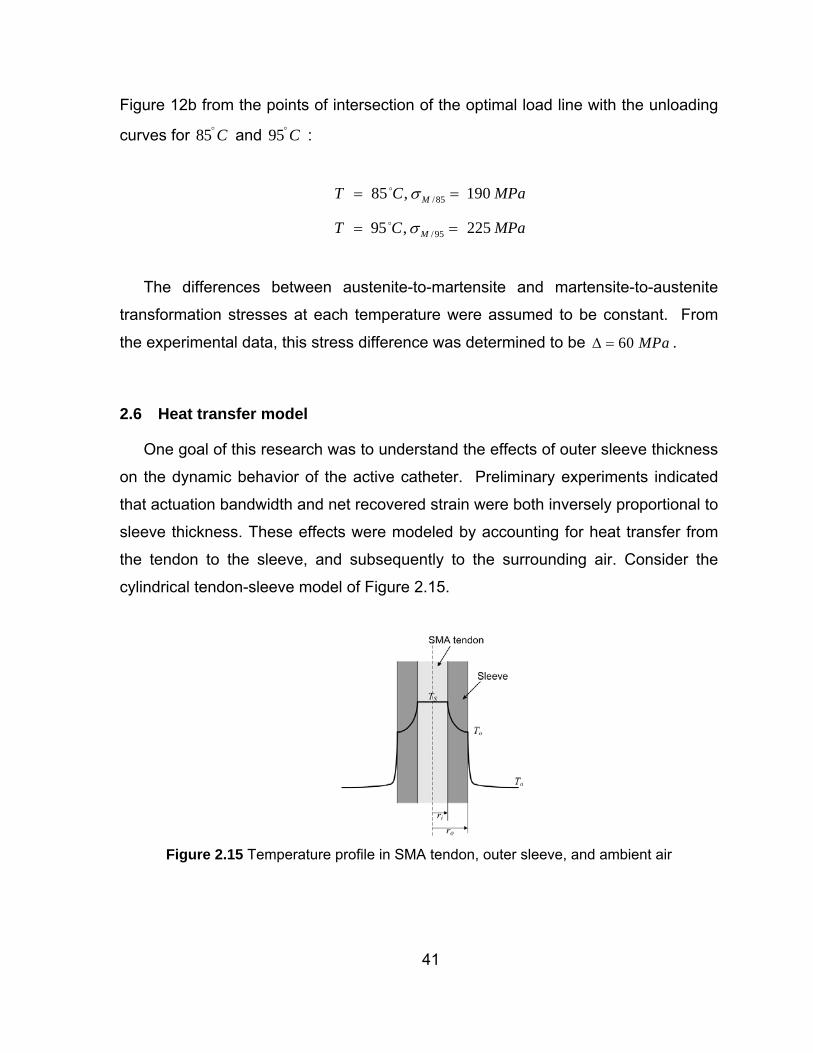
41
Figure 12b from the points of intersection of the optimal load line with the unloading
curves for 85 C° and 95 C° :
/85 85 , 190MT C MPaσ= =
/ 95 95 , 225MT C MPaσ= =
The differences between austenite-to-martensite and martensite-to-austenite
transformation stresses at each temperature were assumed to be constant. From
the experimental data, this stress difference was determined to be 60 MPaΔ = .
2.6 Heat transfer model
One goal of this research was to understand the effects of outer sleeve thickness
on the dynamic behavior of the active catheter. Preliminary experiments indicated
that actuation bandwidth and net recovered strain were both inversely proportional to
sleeve thickness. These effects were modeled by accounting for heat transfer from
the tendon to the sleeve, and subsequently to the surrounding air. Consider the
cylindrical tendon-sleeve model of Figure 2.15.
Figure 2.15 Temperature profile in SMA tendon, outer sleeve, and ambient air

42
An integral formulation can be used to model the temperature dynamics, which
are temporally and spatially dependent [67]:
( ) ( ) ( )( )2
0
( , ) o
i i
r
o o a o o o ar r r
d Gc G r t T rl dr d k A r hA r T Tdt r
π
ρ θ=
⎡ ⎤ ∂⎛ ⎞− = − − −⎢ ⎥ ⎜ ⎟∂⎝ ⎠⎢ ⎥⎣ ⎦∫ ∫ (2.20)
where
oρ =density of outer sleeve ( )3kg m
oc = heat capacity of outer sleeve ( )/J kgK
( , )G r t = temperature as a function of radius and time ( K )
aT = temperature of ambient air ( K )
oT = temperature on surface of outer sleeve ( K )
( )A r = area of cylindrical surface of radius r ( 2m )
ok = thermal conductivity of outer sleeve ( )/W mK
h = convective heat transfer coefficient between outer sleeve and ambient air
( )2/W m K
To facilitate a solution, we make two assumptions [67]. First, we assume the
SMA temperature to be a product of two independent functions of radius and time:
( ) ( ), ( )G r t r T t= Γ
Second, we assume that the spatial temperature distribution resembles its steady
state profile:
1 2( ) lnr c r cΓ = +

43
where:
( )1 lns o
i o
T Tcr r−
=
( ) ( )( )2
ln lnln
o i a o
i o
T r T rc
r r−
=
Based on these assumptions, (2.20) can be evaluated:
( ) ( ) ( )( )2
1 20
ln o
i i
r
o o a o o o ar r r
d Gc c r c T rl dr d k A r hA r T Tdt r
π
ρ θ=
⎡ ⎤ ∂⎛ ⎞+ − = − − −⎢ ⎥ ⎜ ⎟∂⎝ ⎠⎢ ⎥⎣ ⎦∫ ∫
( )
2 2 2 2
1 21 12 ln ln 2
2 2 2 2 2
2 2ln( / )
o i o io o o i o o
s oo o o a
o i
r r r rc l r r c c l c
T Tk l hr l T Tr r
πρ πρ
π π
⎡ ⎤ ⎛ ⎞−⎛ ⎞ ⎛ ⎞⇒ − − − + ⎜ ⎟⎜ ⎟ ⎜ ⎟⎢ ⎥⎝ ⎠ ⎝ ⎠⎣ ⎦ ⎝ ⎠
⎛ ⎞−= − −⎜ ⎟
⎝ ⎠
( )1 1 2 2 2 2ln( / )
s oo o a
i o
T Ta c a c kl hr l T Tr r
π π⎛ ⎞−
≡ + = − −⎜ ⎟⎝ ⎠
where:
2 2
11 12 ln ln
2 2 2 2o i
o o o ir ra c l r rπρ⎡ ⎤⎛ ⎞ ⎛ ⎞= − − −⎜ ⎟ ⎜ ⎟⎢ ⎥
⎝ ⎠ ⎝ ⎠⎣ ⎦
2 2
2 22
o io o
r ra c lπρ⎛ ⎞−
= ⎜ ⎟⎝ ⎠

44
and:
( )1 lna o
i o
T Tcr r−
=
( ) ( )2ln( ) ln( )
ln lni o
o si o i o
r rc T Tr r r r
= −
Substituting for 1c and 2c :
( ) ( ) 1 2
2 1 2 1 2 1
2 ln /- - ln-2 - - -ln - ln - ln -
o i os o oo o a s
i i i
hr l r rT T a a rT kl T T Ta r a a r a a r a
ππ
⎛ ⎞ ⎛ ⎞= ⎜ ⎟ ⎜ ⎟
⎝ ⎠ ⎝ ⎠ (2.21)
(2.21) describes the temporal variation of the temperature on the surface of the
sleeve in response to temperature changes in the SMA tendon. This model provides
a superior representation of the heat transfer than a lumped convective heat transfer
term.
To experimentally investigate the effects of outer sleeve thickness on actuation
bandwidth and amplitude, experiments were conducted using an activated nitinol
specimen and the test rig of Figure 2.16. Here, a SMA specimen was loaded with a
known mass (200 grams) and actuated using a constant current of 0.25A. Mass
displacements were measured using an optical displacement sensor (Philtec RC89)
for a variety of Teflon sleeve thicknesses (0-0.5 mm).

45
Figure 2.16 Setup for investigating effects of outer sleeve thickness
A bare nitinol specimen at room temperature ( 297K ) was loaded with a 200g
mass, resulting in a tensile strain of 5.0% . Vertical displacement of the mass
(extension of the tendon) was monitored while a DC current of 0.25A was applied.
Identical tests were conducted for tendons wrapped with Teflon sleeves of varying
thickness.
Figure 2.17 compares the transient responses of each case.

46
Figure 2.17 SMA displacement responses vs. sleeve thickness
These experimental results reveal that sleeve thickness significantly affects the
transient response characteristics. Not only does the response become slower with
increasing sleeve thickness, but the net strain recovery is also reduced. This could
be attributed the higher heat loss in the SMA tendon with a thin sleeve around it
compared to the convective heat loss of the bare SMA tendon. The critical insulation
thickness at which maximum heat transfer takes place can be estimated as:
0.2 4.4445cr
kr mmh
= = =
This is still much larger than the range of sleeve thicknesses used and hence the
heat loss increases with increasing sleeve thickness. Higher heat loss would imply
slower heating, lower steady state temperatures, and consequently slower and
shorter strain recovery. These effects are effectively captured in the heat transfer
model described before.

47
2.7 Complete single-segment catheter model
The equations associated with tube bending (2.8), SMA phase transformations
(2.10)-(2.16), and heat transfer (2.21) were incorporated into a SIMULINK model to
study the dynamic behavior of the active catheter system. Because this problem is
numerically stiff, the ODE15s solver was selected for numerical integration.
The initial conditions for x+ and x− were specified according to the pre-strain in
the SMA tendon ( 4.25% corresponds to 0.9x+ = and 0.1x− = ), and the initial SMA
temperature sT was assumed to be ambient (297 °C). Many of the model
parameters (e.g. tendon length and outer sleeve thickness) were directly measured
from system components. Other parameters (e.g. heat capacity and thermal
conductivity of outer sleeve) were taken from appropriate reference materials.
Several of the constitutive parameters associated with the SMA tendon were
determined from experimental stress-strain measurements described in Section 2.4.
Physical parameters used in catheter bending model are summarized in Table 2.1.
Table 2.1 Physical constants and parameters of the active catheter prototype
Parameter Symbol Value Source
Density of SMA sρ 36500 /kg m [68]
Resistivity of martensitic phase ,λ+ − 6.997 7− Ωe m [68]
Resistivity of austenitic phase Aλ 8.492 7− Ωe m [68]
Elastic modulus of austenitic phase AE 70.0 GPa [40]
Elastic modulus of martensitic phase ME 30.0 GPa [40]
Relaxation time of SMA τ 0.01 s [40]
Layer volume of SMA micro-structure SV 30.01m [40]
Heat capacity of SMA sc 500 /J kgK [40]

48
Table 2.1 Continued
Elastic modulus of central tube E 70 GPa [40]
Martensitic stress barrier at 85 °C /85Mσ 190 MPa Figure 2.13
Martensitic stress barrier at 95 °C /95Mσ 225 MPa Figure 2.13
Difference between martensitic and
austenitic stress barriers Δ 60 MPa Figure 2.13
Density of Teflon cρ 32140 /kg m [71]
Heat capacity of Teflon cc 1010 /J kgK [71]
Thermal conductivity of Teflon ck 0.2W mK [71]
Convection coefficient between Teflon
and air h 245W m K Estimated
Length of central tube L 0.132 m Design
Thickness of Teflon sleeve 0 ir r− 0.25 mm Design
Distance of tendon from neutral axis a 1.2 mm Design
Area moment of inertia of central tube I 42.844 15−e m Design
Area of cross-section of tendon A 21.267 8−e m Design
Prestrain in SMA tendon pε 0.0425 Design
2.7.1 Experimental setup for measuring catheter tip response
Experimental dynamic behavior of the catheter was obtained using a dual
camera imaging system setup to measure location of the tip in real-time. Two USB
web cameras (Logitech QuickCam Pro 5000) were used with MATLAB’s Image
Acquisition and Image Processing toolboxes to compute the spatial coordinates of
the catheter tip in real-time (5.0 Hz). The cameras were aligned with orthogonal
planes (the xz and yz planes, Figure 2.18) and two-dimensional data from each

49
camera were combined to determine the 3D coordinates of the catheter tip. To assist
in identifying the catheter tip, the background and catheter body were painted white,
while the catheter tip and base were painted black. The measurement system was
calibrated with known dimensions and checked for repeatability.
Figure 2.18 Two-camera measurement system for tracking 3-D position of catheter tip
2.7.2 Catheter actuation experiments
To analyze the transient behavior of the active catheter system and validate the
dynamic model, bending responses were recorded for a variety of pulsed activation
currents. In the first set of experiments, constant currents ( 0.20 0.32A A− ) were
applied to the catheter (outer sleeve thickness: 0.25mm ) long enough for the bending
responses to reach steady state. The current was then switched off, allowing the
catheter to exhibit its free response behavior. Measured bending angles and SMA
temperatures are presented in Figure 2.19.

50
(a) (b)
(c)
Figure 2.19 Experimental catheter bending responses (a) and SMA temperature responses
(b) for 0.0043 Hz input current pulses (c)
Several interesting observations can be made from these experimental results.
During heating, the average bending time constant (approximately 22.0 seconds) is
much slower than that of the bare SMA tendon shown in Figure 2.17 (approximately
4.0 seconds). This reduction in bandwidth can be attributed to heat transfer through
the outer sleeve as explained previously. During heating and cooling, the initial
bending response is rapid, but slows down considerably. This can be attributed to
the fact that the tendon is not located at the center of the catheter but is offset (by a
distance z ) as shown in Figure 2.20. Because of this eccentricity, thermal transients
are faster where the sleeve is thinner and slower where sleeve is thicker.

51
(a) (b)
Figure 2.20 Simplified cross-section of the catheter with SMA tendon placed (a)
concentrically and (b) eccentrically inside the sleeve
Another observation from Figure 2.19 is that the steady-state free bending
response of the catheter is non-zero. This effect is caused by hysteresis in the SMA,
whereby the material does not return to its original phase fractions, and can be
confirmed by noting the intersection of the optimal load line of Figure 2.13 with the
loading curve.
Temperature responses for the SMA tendon were simulated using the heat
transfer models presented in (2.20)-(2.21) and the parameters listed in Table 1.
Simulated temperature responses are compared with experimental responses in
Figure 2.21. The simulated results of Figure 2.21b do not account for the tendon
eccentricity described above, thus the transient characteristics are not in complete
agreement with the experimental data. Noting that the measured responses of
Figure 2.21a exhibit linear first-order characteristics, improvements in simulation
accuracy can be obtained using parameter estimation and linear models.
Specifically, the thermal dynamics of an eccentrically located tendon can be
modeled as a sum of two first-order transfer functions whose time constants are
proportional to minimal and maximal sleeve thickness. The resulting model has the
form:

52
1 2
1 2
( )( ) 1 1
g gT sj s s sτ τ
= ++ +
(2.22)
where ( )T s and ( )j s represent temperature of the SMA tendon above the
ambient temperature and input power, respectively. 1τ and 2τ represent time
constants proportional to the minimal and maximal sleeve thickness, respectively,
and 1g and 2g are gains. All four constants were identified using parameter
estimation methods to minimize modeling error. The simulated temperature
response for 1 518g = , 2 222g = , 1 3τ = , and 2 20τ = is presented in Figure 2.21c,
which compares quite favorably with the measured response of Figure 2.21a.

53
(a) (b)
(c)
Figure 2.21 Temperature response for 0.00434Hz current pulse: (a) experimental, (b)
simulated using heat transfer model (15-18), (c) simulated using identified model (2.22)
Subsequent experiments utilized higher frequency current pulses (0.1 Hz) for
current amplitudes of 0.26 and 0.30 A. Measured vs. simulated SMA temperature
responses for these higher frequency inputs are presented in Figure 2.22.

54
(a) (b)
Figure 2.22 Temperature response for 0.1 Hz current pulses: (a) experimental, (b)
simulated using identified model (2.22)
The effects of heat transfer (through the outer sleeve) are evident in these
experimental and simulated responses. Initially, the SMA temperature increases
from ambient temperature (297 K) in response to Joule heating, but does not reach
steady-state before the current switches off. Subsequent activation cycles begin at
higher initial temperatures, reaching a steady-state peak of approximately 350 K by
the sixth activation cycle. Similar data from prototypes with varying outer sleeve
thickness (not shown) reveals that this transient behavior is more pronounced for
thicker sleeves, as expected.
The complete active catheter model (with identified heat transfer model (2.22))
was simulated for a variety of electric current inputs. Figure 2.23 compares
experimental and simulated bending responses for low frequency (0.0043 Hz) and
higher frequency (0.1 Hz) current pulses.

55
(a) (b)
(c) (d)
Figure 2.23. Experimental vs. simulated active catheter bending responses: (a) measured
response to 0.0043Hz current pulse, (b) simulated response to 0.0043Hz current pulse, (c)
measured response to 0.1Hz current pulse, (d) simulated response to 0.1Hz current pulse
These plots reveal a strong correlation between experimental and simulated data
in both the forced and free responses, and confirm the accuracy of the active
catheter model. The simulation accuracy is better for lower input frequencies,
precisely replicating the range of bend angles, the transient response
characteristics, and the residual bending angle (approximately 10° ) associated with
the free response.
There are, however, discrepancies in the higher frequency responses. The flat
peaks and valleys in the simulated temperature response result from the single-

56
crystal model (2.10)-(2.16) used to represent a polycrystalline material. This
approximation causes a “dead band” in the strain-temperature relationship where
there is no change in strain for small changes in temperature. In reality, however,
polycrystalline materials have continuously varying transformation temperatures and
don’t exhibit these characteristics in the experimental responses.
In conclusion, the single-crystal approximation is found to be useful in describing
the behavior of single-tendon catheter. However, its extension to multi-tendon case
has certain shortcomings. The necessity to conduct tensile tests on every tendon
used on a catheter to derive model parameters makes the practical implementation
of the model tedious. Further, the use of variable step solvers makes the model less
suitable for real-time application of the catheter. Finally, inaccuracies due to single-
crystal approximations are exacerbated when multiple SMA tendons interact with
each other. These shortcomings motivate the necessity for a model which can run in
real-time and can describe the polycrystalline actuation more accurately. However,
the bending mechanics and the heat transfer analysis performed for the single-
tendon catheter can be readily extended to a multi-tendon catheter.
2.8 Extension of bending mechanics to four-tendon catheter
The circular bending mechanics model for the single-tendon catheter were
derived and experimentally validated in Section 2.3. This model can be readily
extended to multiple-tendon catheters, where the net bending moment is the vector
sum of bending moments created by each tendon. The four-tendon catheter has
two degrees of freedom since it can bend independently in the two orthogonal
planes. For this catheter system, we select θ and ϕ as generalized coordinates,
where [ ]max0,θ θ∈ is the bending angle and ] ],ϕ π π∈ − is the orientation of the
plane in which bending takes place. maxθ is the maximum bending angle achievable
by the catheter, in this case about 90°. According to the nomenclature of Figure

57
2.24, the generalized coordinates ( ,θ ϕ ) can be related to individual tendon lengths
as:
( )sinxzl R a ϕ θ+ = − (2.23)
( )sinxzl R a ϕ θ− = + (2.24)
( )cosyzl R a ϕ θ+ = − (2.25)
( )cosyzl R a ϕ θ− = + (2.26)
where xzl+ , xzl− , yzl+ and yzl− are the instantaneous lengths of tendons causing
actuation in the x+ , x− , y+ and y− directions, respectively. R is the instantaneous
radius of curvature and a is the constant distance of each tendon from the neutral
axis.
The neutral axis length, l , is:
l Rθ= (2.27)
Substituting (2.27) into (2.23), the net change in length ( xzl+Δ ) of the ‘ xz+ ’
tendon is:
( ) sinxz xzl l l aθ ϕ+ +Δ = − = − (2.28)
It follows that:

58
cosyzl aθ ϕ+Δ = − (2.29)
xz xzl l+ −Δ = −Δ (2.30)
yz yzl l+ −Δ = −Δ (2.31)
Figure 2.24 Catheter kinematics
2.8.1 Decoupling catheter dynamics in orthogonal planes
Although the four-tendon catheter prototype is a four-input (power applied to
each SMA tendon), two-output (θ ,ϕ ) system, its dynamics can be assumed to be
decoupled in the two orthogonal (xz and yz) planes. The decoupled planar dynamics

59
are further simplified as being Single-Input, Single-Output (SISO) based on the
power applied to each tendon pair and the projection of the bending angle on that
plane. For a given location of the tip ( θ , ϕ ), the bending angles in the two
orthogonal planes xzθ and yzθ can be obtained as follows.
For pure bending in xz plane:
xzxz
ld
θ +−Δ= (2.32)
Substituting (2.28) into (2.32):
( )sinxzθ θ ϕ= (2.33)
Similarly for bending in yz plane:
( )cosyzθ θ ϕ= (2.34)
Also the actuation inputs in each plane are then split into four actuation signals to
prevent power from being simultaneously applied to both tendons of an antagonistic
pair:
If 0xzu ≥ then xz xzu u+ = and 0xzu− =
else xz xzu u− = and 0xzu+ =
If 0yzu ≥ then yz yzu u+ = and 0yzu− =
else yz yzu u− = and 0yzu+ = .

60
Using the above decoupling scheme, each SISO system can then be treated
separately. The schematic of a decoupled system here on referred to as Planar
Catheter Bending (PCB) system, in the xz plane is shown in Figure 2.25. Here xzP+
and xzP− are the forces generated by the individual tendons while xzM + and xzM −
are the corresponding moments. l is the length of the beam and a is distance
between the tendon and tube centerline.
Figure 2.25 PCB system in xz plane
The beam bending equations for this PCB system following the pure bending
argument of Section 2.3 can be written as:

61
1 xz xzM MR EI
+ −−= (2.35)
where E and I are the elastic modulus and the area moment of inertia of the
tube, respectively.
1 xz xzaP aPR EI
+ −−= (2.36)
Or:
( )1 xz xzaA
R EIσ σ+ −−
= (2.37)
where xzσ + and xzσ − are the stresses in each of the tendons respectively.
Also:
xzlR
θ = (2.38)
Hence:
( )xz xz
xz
aAlEI
σ σθ + −−
= (2.39)
Using (2.32):

62
( )p xz
xz
ld
ε εθ +−
= (2.40)
where pε is the prestrain and xzε + is the instantaneous value of strain of the xz+
tendon.
From (2.39) and (2.40):
( ) 2
( )p xzxz xz
EIa A
ε εσ σ +
+ −
−− = (2.41)
Denoting the effective stiffness due to the tube as:
2tubeEIK
a A= (2.42)
Hence, the effective equation for the PCB system is obtained as:
( ) ( )xz xz tube xz pKσ σ ε ε+ − +− = − − (2.43)
This equation can also be written in terms of strain in the xz− tendon using the
relation:
p xz xz pε ε ε ε+ −− = − (2.44)

63
This is because the strain recovered in one tendon is exactly equal to the strain
added to the other tendon. Substituting (2.44) in (2.43), we get:
( ) ( )xz xz tube xz pKσ σ ε ε+ − −− = − (2.45)
Similar equations can be obtained for the yz plane using the above derivation.
2.8.2 Occurrence of slack in the PCB system
It should be noted that the tendons in the antagonistic configuration of the PCB
system can develop slack under certain conditions. For example, consider a case
where the xz+ tendon is actuated via Joule heating it and then left to cool (Figure
2.26). This actuation process will cause the catheter to bend towards the x+direction while also causing the xz− tendon (which is at room temperature) to
extend passively. During the cooling phase, the catheter returns towards its neutral
position. However, during this phase the xz− tendon sees a compressive stress.
Because of its thin diameter, the tendon tends to buckle instead of being
compressed and offers negligible resistance (zero stress in the tendon with slack) to
the catheter returning towards neutral position. This buckling in the passive tendon
appears as “slack”: an additional nonlinearity which needs to be to considered while
modeling the PCB system with anatagonistic SMA tendons. Hence, any subsequent
actuation of the xz− tendon will first recover the slack in the tendon before causing
bending of the catheter in the x− direction.

64
(a) (b) (c)
Figure 2.26 Slack development in SMA tendons: (a) neutral position, (b) xz+ tendon
actuated, and (c) appearance of slack in the xz− tendon

65
Chapter 3. Hysteretic Recurrent Neural Networks
3.1 Introduction
In the previous chapter, SMA actuation was modeled using the Seelecke-Muller-
Achenbach model [39] for single-crystal materials. Although this energy-based
model has several advantages over other approaches, it also has shortcomings that
limit its applicability to the real-time catheter control. The single-crystal SMA model is
difficult to apply to the polycrystalline, multi-tendon nature of the robotic catheter.
Heintze, et. al [37] describes a method to extend the model to polycrystalline
materials, but because it requires a priori knowledge of all system states it is clearly
unsuitable for this application. Furthermore, the single-crystal model uses variable-
step solvers which are not ideal for real-time control implementations. In view of
these shortcomings, a polycrystalline modeling approach is sought which accurately
captures the hysteretic nature of SMA tendons and is easily incorporated into a real-
time control architecture.
Apart from the modeling approaches discussed in the previous chapter, there is a
significant amount of literature regarding modeling approaches for general hysteretic
systems. Hysteresis is a phenomenon commonly encountered in smart materials
(including magnetostrictives, ferroelectrics, piezoelectrics and shape memory
alloys), hence there have been major research efforts into developing a general
framework for modeling hysteresis. One popular mathematical description of
hysteresis is the Preisach model, which is frequently used in ferromagnetic
modeling. The Preisach model established the convention of using individual
hysteretic operators, or hysterons [46], to represent non-ideal relays. Each operator
is parameterized by a forward transition value α and a reverse transition value β .
The output of each operator ,α βγ is a Boolean value corresponding to one of two
states, as illustrated in Figure 3.1.

The
In
weig
The
oper
output of ea
n its discr
hted opera
density fu
ator (,i iuα βγ
Fig
ach operato
,iα βγ
rete implem
tors:
nctions (μ α
)( )u k ; thes
gure 3.1 Illus
or is determ
( )( )i
u ku
β
⎧⎪= ⎨⎪⎩
mentation,
( )( )Pf u k =
, )i iα β , also
se weights
66
stration of a
mined by th
1 1 if uif
unchanged if−
the Preisa
1( , )
N
i ii
μ α β γ=∑
o known a
can be so
Preisach op
e input con
( )( ) ( )
i
i
i
u ku kif u k
αβ
β
><≤ ≤
ach output
( ),) ( )i i
u kα βγ
as Preisach
olved analy
perator
nditional sta
iα≤
t Pf is a
h measures
ytically or
atement:
(3
summatio
(3
s, weight e
estimated
3.1)
n of
3.2)
each
from

67
experimental data. As expected, the accuracy of this discrete model increases with
the number of operators. The Preisach model implements a directional input
dependence (or memory) based on a “wiping out” property, where the relevant curve
depends on the extrema of all previous inputs. A new extremum “wipes out” any
previous smaller extrema. Therefore, as part of the Preisach model, an algorithm
must be implemented that stores these relevant points. For a complete description of
the Preisach model, see [46] or [47]. This model and similar derivations have been
implemented successfully in control algorithms for hysteretic systems [45, 48, 49].
Alternative approaches to modeling hysteresis include various implementations
of artificial neural networks (ANNs). ANNs are useful tools for modeling
nonlinearities because of their “universal approximation” capabilities: they can
approximate any nonlinear function with arbitrary accuracy [50,51]. Furthermore,
ANNs can be readily adapted to account for parameter variations. ANNs are based
on weighted sums of interconnected processing elements called neurons. Common
nonlinear activation functions include sigmoids and radial basis functions.
Different types of ANNs have been used to model hysteresis. Feed-forward
neural network (FFNN) implementations are common in the literature, and benefit
from an abundance of available training algorithms. However, to capture requisite
directional input dependence, time-delayed input sequences or binary tags indicating
directional information must be provided to the ANN [52,53]. This limitation of FFNNs
can be overcome using recurrence, where the input includes feedback of one or
more network outputs. In fact, recurrent neural networks (RNNs) have inherent
memory capabilities very relevant to hysteretic modeling. This memory is achieved
through the use of context layers, which contain feedback connections from either
the output layer or hidden layers. The possibilities are only limited by the need for
computational efficiency. Examples of recurrent neural networks include Elman and

68
Hopfield neural networks [54]. Various researchers have combined neural networks
with Preisach models for greater accuracy and density function optimization [55].
In this chapter, a novel derivation of a hysteretic recurrent neural network
(HRNN) is described. Instead of using the ANN to determine the weights of Preisach
operators, the network incorporates a hysteretic neuron consisting of conjoined
sigmoid activation functions. Although similar hysteretic neurons have been explored
previously, most implementations require that neuron hysteresis be determined by
differentiating the inputs [56], by creating two families (for rising and falling inputs) of
parameterized activation functions [57] or by using the applicable maximum and
minimum extrema [58]. Using simple recurrence, we create neurons that self-select
the relevant activation functions. Furthermore, training is facilitated by placing the
network weights on the output side, allowing standard backpropagation of error
(BPE) training algorithms to be used.
This chapter also discusses various applications starting from simple two-phase
systems to more complex three-phase systems. A two-phase HRNN is described
first, and is used to model phase transformations in a ferromagnetic material. The
two-phase HRNN is also used to model the SISO actuation of a mass suspended by
an SMA wire. A three-phase HRNN is used to model the stress-strain characteristics
of an SMA wire over a range of temperatures. Because the robotic catheter uses
multiple tendons and obtaining stress-strain characteristics for each and every
tendon is a cumbersome process, methods for training a three-phase HRNN based
solely on a system’s output response are developed. Such a method is first
demonstrated for the SISO actuation of a mass suspended by an SMA wire. It is
then extended to a multivariable system consisting of a catheter actuated by two
antagonistic SMA tendons.

69
3.2 Hysteretic Recurrent Neural Network
Like the Preisach model of [46], the hysteresis neuron in the HRNN is motivated
by a two-phase constitutive relationship, such as the magnetic domains of
ferromagnetic materials or the electric dipoles in piezoelectric materials. The neuron
consists of conjoined forward and reverse activation functions, specified by forward
and reverse transformation thresholds iα and iβ , respectively (Figure 3.2).
Figure 3.2 Hysteretic kernel consisting of conjoined sigmoid activation functions
Although this neuron resembles the Preisach operator of (3.1), its uniqueness
lies in the determination of directional input dependence. Instead of implementing
algorithms external to the ANN or requiring historical input data, selection of the
appropriate activation function is achieved using recurrence at each hidden layer
neuron. The activation function for each neuron is described using the difference
equation:
( ) ( )( ) ( )( )1 ( 1) ( 1)1 1i i i i
i ii u k u k
f k f kf ke eα χ β χ− −
− − −= +
+ + (3.3)
where ( )if k and ( )1if k − are the present and previous outputs of the thi neuron,
( )u k is the present input, and iα and iβ are the forward and reverse transformation

70
values, respectively. iχ is a sigmoid loop shaping parameter typically set to a large
value ( )1iχ to approximate a step function. The output ( )if k represents the
probability that the neuron exists in one of the two phases. According to this
formulation, if the neuron was previously inactive ( ( )1 0if k − = ), then an output
transformation will follow the forward activation function, activating if ( ) iu k α≥ .
Conversely, if the neuron was previously active ( ( )1 1if k − = ), then an output
transformation will depend on the reverse activation function, de-activating if
( ) iu k β≤ . This recurrence enables self-selection of the appropriate activation
function, eliminating the need for context units or conditional statements which tend
to complicate training.
The output of the HRNN, ( )y k , is the weighted sum of N neurons:
2
1 1
ˆ ( ) ( )N N
i i ii i
y k w f kφ= =
= =∑ ∑ (3.4)
The architecture of the HRNN is presented in Figure 3.3.

contr
phys
analo
repre
spec
differ
mode
mode
upda
Marq
Fig
By squa
ributions fr
sical mater
ogous to
esents the
cific neuron
rent fraction
el and mo
el [59].
Standard
ate the netw
quardt algo
ure 3.3 Hys
aring the n
rom each h
rial. For ex
individual
portion of
. The sum
ns is unity.
re like a p
d backprop
work weigh
rithm (LMA
steretic Recu
network we
hysteretic n
xample, if
crystals in
the macro
of all 2iw i
In this man
parameteriz
agation of
ts. For the
A) is used [
71
urrent Neura
eights, the
neuron, ma
one views
a smart
oscopic ma
is normaliz
nner, the H
zed model
error (BPE
results pre
[60]. A qua
al Network (H
e training p
aintaining a
s the hyst
material s
aterial that
zed to ensu
RNN resem
of the actu
E) training a
esented in t
adratic cost
HRNN) archi
process en
a statistica
teretic neu
specimen,
can be rep
ure that the
mbles less o
ual system
algorithms
this paper,
function is
itecture
nsures pos
al model of
urons as b
then each
presented
e sum of al
of a “black
, or “grey
can be use
the Levenb
s defined ba
sitive
f the
being
h 2iw
by a
ll the
box”
box”
ed to
berg-
ased

72
on the accumulated error between the desired output ( )y k and the HRNN predicted
output ˆ ( )y k over K input-output samples:
2
1
1 ( )2
K
kV e k
=
= ∑ (3.5)
where the residuals are:
ˆ( ) ( ) ( )e k y k y k= −
(3.6)
The weight update [ ]1 2T
Nw w w= Δ Δ ΔΔw is given by:
1( )T Tμ −= − +Δw J J I J e (3.7)
where I is the N N× identity matrix, μ is a positive damping factor, and J is the
K N× Jacobian of the error cost function, defined as:
,
( ) 2 ( )k i i ii
e kJ w f kw
∂= = −
∂ (3.8)
The weights are then updated, according to:
new old= +Δw w w
(3.9)
After the weights are updated, each 2iw is normalized using:

73
1/2
2
2
1
ii N
ii
www
=
⎛ ⎞⎜ ⎟⎜ ⎟=⎜ ⎟⎜ ⎟⎝ ⎠∑ (3.10)
3.3 Modeling magnetic hysteresis
To demonstrate the HRNN’s ability to model hysteresis, a simple magnetic circuit
was constructed (Figure 3.5). Hysteresis is a well known characteristic of
ferromagnetic materials. In fact, B-H curves often serve as classic illustrations of
hysteresis. The magnetic core was fabricated from pure iron with 300 turns of 18
gauge magnet wire. A digital gaussmeter (Magnetic Instrumentation Model 912)
connected to a PCI multifunction data acquisition device (National Instruments PCI
6024E) is used to measure the magnetic flux density at a sampling rate of 20 Hz.
Coil current was controlled using a programmable power supply (Kepco BOP 100-
2M) and the same data acquisition (DAQ) hardware. A piecewise linear alternating
current input was used to capture the first-order ascending and descending
transition curves. Figure 3.4 and Figure 3.5 present a schematic and photograph of
the experimental setup. Figure 3.6 shows typical input-output measurements
obtained from the experimental setup.

Figure 3.4
Figure 3.5
4 Schematic
Photograph
of the expe
h of the expe
74
rimental set
erimental set
up for meas
tup for meas
suring magne
suring magn
etic hysteres
netic hystere
sis
esis

75
(a) (b)
Figure 3.6 Experimental input (a) and output (b) data acquired from the setup
This experimental B H− data was normalized and divided into a training set
(850 input-output samples) and a validation set (212 input-output samples). A
HRNN with 404 neurons was initialized with forward transition values α ranging
from 0 to 1 at .01 intervals (resulting in 101 discrete forward transition values). Each
forward transition value has four different reverse transition values associated with it,
with differences ranging from 0.02 to 0.47. For example, each α has reverse
transition values equal to 0.02α − , 0.17α − , 0.32α − and 0.47α − . The Levenberg-
Marquardt training algorithm was implemented using MATLAB’s LSQNONLIN
function (The Mathworks, Inc., Natick MA), and the HRNN is trained for 11 epochs,
at which point the validation cost began to increase (Figure 3.7a). During this training
interval, the training cost reduced from 1.05·10-2 to 1.78·10-5, while the validation
cost reduced from 1.06·10-2 to 2.51·10-5. Figure 3.7 compares HRNN predictions to
normalized experimental data for training data. For clarity, the ascending transition
data (Figure 3.7b) is presented separately from the descending transition data
(Figure 3.7c).

76
(a)
(b) (c)
Figure 3.7 HRNN training results: (a) cost functions during training; (b) comparison of
training data vs. HRNN predictions for ascending transitions; (c) comparison of training data
vs. HRNN predictions for descending transitions
The HRNN has accurately characterized the major hysteresis loop and the first-
order ascending and descending transition curves.
For comparison purposes, a radial basis function network (RBFN) was created
using MATLAB’s Neural Network Toolbox. This RBFN was trained using the same
experimental input-output data as the HRNN. In order to capture the directional
dependence of the system, the inputs to the RBFN included current and delayed

77
inputs, ( )u k and ( )4u k − respectively, and delayed output ( )4y k − . This
combination of present and delayed inputs was found to provide the best results
based on numerous simulations involving different numbers and types of inputs. The
input time delay ( 4k − , corresponding to 2.0 seconds) is a critical design parameter
that must be optimized; large time delays hinder the RBFN’s ability to model minor
hysteresis loops, while small time delays hinder its ability to differentiate the data
from noise. While more advanced techniques exist for designing and training ANNs,
this three-input RBFN represents a reasonable comparison to the HRNN in terms of
network sophistication. In fact, significantly more time was spent optimizing the
RBFN in order to achieve performance comparable to the HRNN.
The spread of the radial basis functions is set to 0.2. The RBFN is trained until
the number of neurons (407) was approximately equal to the number of neurons in
the HRNN. For this reason, the training results of Figure 3.8 do not include validation
data.
(a) (b) Figure 3.8 RBFN training results: (a) comparison of training data vs. network predictions
for ascending transitions; (b) comparison of normalized training data vs. network predictions
for descending transitions

78
Comparing the results of Figure 3.7 and Figure 3.8 seems to indicate that both
the HRNN and the RBFN have captured the hysteretic characteristics of the
magnetic circuit with similar accuracy. In fact, the final training cost functions for the
HRNN and RBFN were 1.78·10-5 and 8.14·10-7, respectively. However, the true
modeling capabilities of each network can only be assessed using test data:
normalized experimental data not utilized for training (Figure 3.9a and Figure 3.9b).
Note that the time rate of change of the input current in Figure 3.9a is slower than
the rates in Figure 3.6 (0.1 A/s vs. 0.12-0.2 A/s, respectively). Figure 3.9c and
Figure 3.9d compare the HRNN and RBFN outputs to test data acquired from the
magnetic test rig.

79
(a) (b)
(c) (d)
Figure 3.9 HRNN and RBFN test results: (a) test input data; (b) test output data; (c)
comparison of test data vs. network predictions; (d) comparison of test error for both
networks
For this new test data, the HRNN’s error cost function is slightly higher than its
training cost: 4.45·10-4 vs. 1.78·10-5, respectively. However, the RBFN’s test cost is
orders of magnitude higher than its training cost: 17.43 vs. 8.14·10-7, respectively.
These results clearly illustrate the HRNN’s superior ability to generalize a
hysteretic system using a relatively small number of neurons and a simple training

80
method. The HRNN excels because of its inherent ability to generalize transitions,
regardless of changes in the rate of input. The RBFN fails to generalize because of
its reliance on time delayed inputs. For a system where the temporal response is
negligible, such as the magnetic circuit, the reliance on the time step between inputs
to the network is significant. Furthermore, the RBFN fails to capture minor loops and
reversals not included in the training data, like the reversals occurring after
approximately 100 seconds in Figure 3.9, yielding significantly higher error.
3.4 Modeling two-phase transformations in SMA
To demonstrate the HRNN’s generalization capabilities with asymmetric
hysteretic loops and process noise, we extend this modeling approach to two-phase
transformations in shape memory alloy (SMA) materials. Although general SMA
actuation processes exhibit three distinct crystal phases ( A , M+ and M− ), it is
possible to isolate actuation processes involving only two-phase transitions. One
such process involves actuation under a relatively high constant stress, where
crystals transform between the M+ phase at low temperatures to the A phase at
high temperatures. For this reason, several published models account for only these
phases and neglect the third [62].
To demonstrate the modeling process for a two-phase SMA actuator, a test rig
was built to maintain constant tension on a temperature-controlled SMA wire (Figure
3.11). A 0.127 mm diameter NiTi wire (Dynalloy, Inc., Costa Mesa, CA) was bonded
to stainless steel anchors (hypodermic tubing, 1.06 mm OD x 0.762 mm ID x 5.08
mm length) at each end. The wire was secured to the test rig by locking the top
anchor into a nylon collet. A 25 mm dia steel ball bearing (m=0.0663 kg) is secured
to the lower end of the SMA wire using a second collet, creating a static stress of
5.29·107 Pa in the material. Joule heating of the SMA wire was achieved using a
current-controlled programmable power supply (Kepco BOP 100-2M). The
displacement of the suspended mass was monitored using an infrared sensor

(Philt
therm
cond
Cem
using
tec RC89
mocouple (
ductive, ele
ment). All ex
g a PCI mu
Figure
Figure
), and te
(Omega C
ectrically n
xperimenta
ltifunction d
e 3.10 Schem
3.11 Photog
mperature
CHAL-002)
non-conduc
l data was
data acquis
matic of expe
graph of exp
81
was mo
bonded to
ctive ceme
acquired a
sition device
erimental se
perimental se
nitored us
o the SMA
nt (Omega
at a consta
e (National
etup for meas
etup for mea
sing a mi
A wire usin
a CC High
ant sample
Instrument
suring SMA
asuring SMA
iniature K-
ng a therm
h Tempera
rate of 0.4
ts, Austin T
hysteresis
A hysteresis
-type
mally
ature
4 Hz
TX).

82
As before, a piecewise linear alternating current was used to capture the first-
order ascending and descending transition curves in the SMA. Figure 3.12 shows
typical input-output measurements obtained from the experimental setup.
(a) (b)
(c)
Figure 3.12 Experimental training data acquired from the SMA test rig: (a) input current,
(b) SMA surface temperature, (c) SMA displacement

83
Additional validation data was acquired to obtain higher order transition curves
(Figure 3.13).
(a) (b)
(c)
Figure 3.13 Experimental validation data acquired from the SMA test rig: (a) input
current, (b) SMA surface temperature, (c) SMA displacement
To model this SMA actuator, a HRNN with 909 neurons was initialized. The
normalized forward transition temperatures were uniformly distributed from 0 to 1 at
intervals of 0.01, yielding 101 values. The differences in the forward and reverse
transition temperatures ranged from 0.0 to 0.4 at intervals of 0.05, giving 9 values for
each forward transition and a total of 909 neurons.

84
The experimental training data (1761 input-output samples, Figure 3.12) and
validation data (1325 input-output samples, Figure 3.13) were normalized, and the
HRNN was trained for 25 epochs (the point at which the validation cost function
begins to increase, as shown in Figure 3.14a). During this training interval, the
training cost reduced from 1.50·10-2 to 8.03·10-5, while the validation cost reduced
from 1.63·10-2 to 4.23·10-4. Figure 3.14 compares HRNN predictions to
experimental data for training and validation data. For clarity, the ascending
transition data (Figure 3.14a) is presented separately from the descending transition
data (Figure 3.14b). A comparison of the experimental validation data and the HRNN
prediction is shown in Figure 3.14c.

85
(a)
(b) (c) Figure 3.14 HRNN training results: (a) comparison of training data vs. HRNN predictions
for ascending transitions; (b) comparison of training data vs. HRNN predictions for
descending transitions; (c) comparison of validation data vs. HRNN predictions
These results clearly demonstrate the HRNN’s modeling capabilities for two-
phase hysteretic materials. The HRNN captures the major loop as well as ascending
and descending branches of the minor loops.
As noted previously, by constructing a “grey box” neural network model to
replicate the physical system, one can glean important statistical information about
the material. For example, by looking at the weights of each neuron, the proportions
of crystals in the SMA transitioning at the forward and reverse values can be

86
determined. Figure 3.15 shows that the majority of forward transitions occur between
50 °C and 70 °C, while the reverse transitions occur between 30 °C and 50 °C.
These HRNN model results are consistent with the experimental data. The steep
slopes of Figure 3.14b and Figure 3.14c indicate regions where most of the
transitions occur; the forward transitions occur on the right side, while the reverse
transitions occur on the left side. A careful inspection of these experimental results
confirms that the majority of the forward transitions occur between 50 °C and 70 °C
and the majority of the reverse transitions occur between 30 °C and 50 °C.
(a) (b)
Figure 3.15 Weights of the neurons for the forward transition values (a); Weights of the
neurons for the reverse transition values (b)
3.5 Modeling three-phase transformations in SMA
In the previous section, SMA actuation was described in terms of transformations
between two crystal phases; more general SMA-actuated systems (like the robotic
catheter) require full transformation descriptions between all three phases. As
discussed previously, the unique properties of SMA can be attributed to the
presence of three crystal phases: austenite ( A) and two martensite variants ( M+ and
M− ). However, for the special case of tensioned wire actuators, we can consider the

87
material to be composed of detwinned martensite ( M+ ) and twinned martensite (
/M+ − ) instead of M+ and M− , since the actuator is not expected to undergo any
compressive stresses where the M− phase could exist independently. This is an
important simplification that restricts the operating region of SMA exclusively to
tensile stresses and strains and it will be adopted for the remainder of this chapter.
Modeling transformations between these three phases requires modifications to
the HRNN model of (3.3). The hysteretic neuron can be modified to include two
difference equations (instead of one) and two inputs (internal temperature and stress
or strain). The characteristics of this three-phase neuron are consistent with the
Seelecke-Muller-Achenbach single-crystal model [37]. However, the inherent
recurrence of the HRNN makes it computationally efficient, enabling its direct
extension to polycrystalline materials and excellent approximation based on
experimental data.
Modeling a polycrystalline SMA wire actuator in terms of three-phase hysteretic
neurons, each representing single-crystal SMA (SCSMA) elements, can be
accomplished using either series or parallel combinations of the SCSMA elements
(Figure 3.16). The choice of series or parallel representations depends on the
specific application, as one approach might be significantly easier to implement than
the other.

88
,σ ε
1,σ ε
2,σ ε
, Nσ ε
1,σ ε 2 ,σ ε ,Nσ ε
(a) (b) Figure 3.16 Representation of polycrystalline SMA specimen as a parallel (a) or series
(b) combination of SCSMA elements
When an SMA wire actuator is represented as a parallel combination of SCSMA
elements, the strain on each SCSMA element is the same as the whole wire, while
the total wire stress is a weighted sum of SCSMA element stresses. Thus, the inputs
to each hysteretic neuron representing a parallel SCSMA element are strain and
temperature (making it a “strain-based” neuron), while the output is stress.
Conversely, when an SMA wire actuator is represented as series combination of
SCSMA elements, the stress on each SCSMA element is the same as that for the
whole wire. In this case, the total wire strain is a weighted sum of SCSMA element
strains. Thus, the inputs to each hysteretic neuron representing a series SCSMA
element are stress and temperature (making it a “stress-based” neuron), while the
output is strain.
3.5.1 Stress-based HRNN
The stress-based neuron contains two internal variables: [ ], 0,1A ix ∈ and
[ ], 0,1M ix+∈ where i is the neuron index (1 i N≤ ≤ ). Each variable represents the
probability that the neuron exists in a specific phase ( A and M+ , respectively). The
probability of existing in the third phase is simply:

89
/ , , ,1M i A i M ix x x+ − +
= − − (3.11)
These phase probabilities are determined from the outputs of two difference
equations, , ( )M if k+
and , ( )A if k . The first equation relates internal stress to the M+
phase:
, , , ,
, ,, ( ( )) ( ( ))
1 ( 1) ( 1)( )
11 f i i m r i i m
M i M iM i k k
f k f kf k
ee σ σ χ σ σ χ+ +
+ − −
− − −= +
++ (3.12)
where ( )kσ is the internal stress, ,f iσ is the forward transformation stress, ,r iσ is
the reverse transformation stress, and ,i mχ is the loop shaping parameter. Thus a
neuron is determined to be in M+ phase if the applied stress is higher than forward
transformation stress; it stays in the M+ phase until the stress drops below the
reverse transformation stress.
A second equation relates internal temperature to the A phase:
, , , ,
, ,, ( ( )) ( ( ))
1 ( 1) ( 1)( )
11 f i i a r i i a
A i A iA i T T k T T k
f k f kf k
ee χ χ− −
− − −= +
++ (3.13)
where ( )T k is the internal temperature, ,f iT is the forward transformation
temperature at which the neuron transforms from /M+ − into the A phase, ,r iT is the
reverse transformation temperature at which the neuron transforms back into /M+ −
phase and ,i aχ is the loop shaping parameter.
The phase probabilities are determined from difference equations:

90
, ,( ) ( )M i M ix k f k+ +
= (3.14)
( ), , ,( ) 1 ( ) ( )A i M i A ix k f k f k+
= −
(3.15)
( )( )/ , , ,( ) 1 ( ) 1 ( )M i M i A ix k f k f k
+ − += − −
(3.16)
The rationale behind this formulation is as follows. According to (3.12), having
, ( ) 1M if k+
= (which can occur at high stresses) excludes the possibility of the neuron
existing in either the A or /M+ − phase ( , 0A ix = and / , 0M ix
+ −= ). However, when
, ( ) 0M if k+
= (which can occur at lower stresses), the neuron can exist in either the A
or /M+ − phase, as specified by (3.13). Consistent with other models [39], the
transformation stresses ,f iσ and ,r iσ are assumed to vary linearly with temperature:
( )
/, , , , , ,( ) ( 1) (1 ( 1))f i f i f i a i M i a ia T k b f k f kσ σ+ −
= + − + − −
(3.17)
where ,f ia and ,f ib are constants governing the high temperature transformation
from A to M+ , and / ,M iσ
+ − is a constant governing the low temperature transformation
from /M+ − to M+ which is independent of temperature. Specifically, ,f ia is the slope
of the transformation region between A and M+ . As temperature rises, higher
stresses are required to convert a crystal to M+ . The reverse transformation stress
is:
( )( ) ( ) ( ) ( )( )
/ /, , , , , ,1 1 1r i f i f i A i a M i M i aa T k b f k f kσ σ σ σ+ − + −
= + − Δ − + −Δ − −
(3.18)

w
stres
after
estim
w
AE is
show
N
,f iT ,
and
expe
trans
where ,A iσΔ
ss-strain hy
determinin
mate ˆ ( )i kε
where Tε is
s the elasti
wn in Figure
Note that ea
,r iT , ,f ia , b
,r iT ) for th
edite trainin
sformation t
i and Mσ+
Δ
ysteresis lo
ng , ( )A ix k ,
for a given
ˆ ( )i k σε⎛
= ⎜⎝
the total re
ic modulus
e 3.17.
Figure 3
ach neuron
,f i , ,A iσΔ , σ
he two-pha
g, several
temperature
/ ,i+ − are con
oop at high
, ( )M ix k+
an
stress and
( )T
M
k xEσ ε
⎞+ ⎟
⎠
ecoverable
s for austen
3.17 Three-
in the three
/ ,M iσ+ −
, and
ase HRNN
assumption
es can be a
91
nstants tha
h and low
nd / , ( )M ix k
+ −
d temperatu
,(( )M i
A
kx kEσ
++
strain, ME
nite. A dia
phase, stres
e-phase HR
/ ,M iσ+ −
Δ ) co
N. To redu
ns can be m
assumed to
, ,f i rT T=
at specify t
temperatur
) , the stre
ure is [37]:
,) ( )A i
A
k x kEσ
+
is the elast
gram of th
ss-based HR
RNN depen
ompared to
ce this nu
made. First
o be equal:
i
the width o
res, respec
ess-based
/ ,( ) (M iM
k x kEσ
+ −
tic modulus
he stress-ba
RNN neuron
nds on seve
just two p
umber of p
t, the forwa
of the neu
ctively. Fin
neuron’s s
)k
(3.19
s for marten
ased neuro
en paramet
parameters
parameters
ard and rev
(3.20
ron’s
nally,
strain
9)
nsite,
on is
ters (
( ,f iT
and
verse
0)

92
Next, the linear dependence of transformation stress on temperature (3.17) can
be simplified:
/, , , ,f i f i f i M ib a T σ+ −
= − + (3.21)
This relationship ensures that there are no discontinuities in forward
transformation stress when a neuron transforms from the A or /M+ − phase. It can
also be assumed that:
/ ,M iσ+ −
Δ = , 0A iσΔ > (3.22)
This assumption ensures that there are no discontinuities in reverse
transformation stress and that the reverse transformation stresses are always lower
than the forward transformation stress. Using these assumptions, the seven original
parameters can be reduced to four: ,f iT , ,f ia , ,M iσ + , and iσΔ .
Figure 3.18 illustrates the characteristics of a single three-phase neuron
incorporating these assumptions ( , 45°Cf iT = , 6, 8 10 Pa/ Cf ia = ⋅ ° , 8
, 2 10 PaM iσ + = ⋅ and
82.5 10 i PaσΔ = ⋅ ) for varying loads and temperatures. At low temperatures the
neuron exists in the /M+ − phase for low loads, exhibiting a constant /M+ − to M+ transformation stress until the temperature exceeds 45 °C. Above this temperature,
the neuron transitions into the A phase at low loads, exhibiting a linear A to M+ transformation stress with temperature.

93
Figure 3.18 Stress-strain characteristics simulated using a single stress-based neuron
at different temperatures
The output of the three-phase HRNN (Figure 3.19) is a weighted sum of stress-
based neuron outputs representing the total material strain ˆ( )kε :
2
1
ˆ ˆ( ) ( )N
i ii
k w kε ε=
= ∑ (3.23)
The weights are updated according to the same Levenberg- Marquardt algorithm
described for the two-phase HRNN ((3.5)-(3.9)). As before, the weights are
normalized after each iteration so that the sum of squared weights is unity.

3.5.2
T
a st
nece
(kσ
A
curre
Figur
2 Strain-b
The develop
tress-based
essary. Firs
) is unavai
Additionally,
ent strain by
re 3.19 Thre
ased HRN
pment of a
d neuron.
t, since the
ilable, the s
,M if+
, the stres
y inverting
ee-phase HR
N
strain-base
However,
e stress ass
stress delay
(
1( )
1 f
Mfke σ
−=
+
ss for the
(3.19):
94
RNN architec
ed HRNN n
certain m
sociated wit
yed by a un
, ,
,( 1))
( 1)f i i m
M ik
kσ χ
+
− −
−+
current ite
cture using s
neuron is es
minor chan
th a neuron
nit sample σ
,
,( (
(1 r i
M ik
f ke σ σ
+
− −
−
+
ration mus
stress-based
ssentially s
nges in fo
n at any pa
( )1kσ − m
,1))
1)i mχ
st be estim
d neurons
same as tha
ormulation
rticular itera
must be used
(3.2
mated from
at for
are
ation
d:
24)
m the

95
/
,
,, ,
( ) ( )ˆ ( ) ( )( ) ( )
i T M ii
M iM i A i
M A M
k x kk x kx k x k
E E E
ε εσ +
+ −+
−=
+ + (3.25)
( )T k
, ( )a if k
, ( )M if k+
ˆ ( )i kσ( , )Tσ ε
( )i kε
Figure 3.20 Three-phase, strain-based HRNN neuron
The remaining assumptions and equations derived for the stress-based neuron
hold for the strain-based neuron. The output stress ˆ ( )kσ of the three-phase HRNN
constructed from strain-based neurons is a weighted sum of output strains of each
neuron (Figure 3.21):
2
1
ˆ ˆ( ) ( )N
i ii
k w kσ σ=
= ∑ (3.26)

96
Figure 3.21 Three-phase HRNN architecture using strain-based neurons
3.5.3 Validation of three-phase HRNN
To validate the modeling capabilities of a three-phase HRNN, experimental
stress-strain data from an SMA wire (Chapter 2, Section 2.5) is used. This tensile
test data is sufficient for training because it represents all three SMA phases.
Although this modeling demonstration makes use of 300 stress-based HRNN
neurons (representing SCSMA elements in series), a strain-based (parallel)
representation would be an equally valid and effective approach. The four
parameters for each neuron are initialized with random numbers across the following
ranges: [ ], 25,35f iT ∈ , 6 6, 3 10 ,8 10f ia ⎡ ⎤∈ ⋅ ⋅⎣ ⎦ , 6 8
, 3 10 ,3 10M iσ+
⎡ ⎤∈ ⋅ ⋅⎣ ⎦ , and
7 81 10 ,3 10iσ ⎡ ⎤Δ ∈ ⋅ ⋅⎣ ⎦ . The material parameters in (3.19) are also initialized:
930 10ME = ⋅ , 970 10AE = ⋅ , and 0.053Tε = . Stress-strain data at temperatures of 24
°C, 45 °C, 75 °C, and 95 °C were divided into a training set (217 samples) and a

97
validation set (222 samples). Data from the remaining stress-strain curves (35 °C, 55
°C, 65 °C, and 86 °C) are used as a test set. The HRNN is trained using the
Levenberg-Marquardt algorithm, and the weights are normalized after each epoch.
Every 20 training epochs, the neurons with the lowest weights are re-initialized and
the neurons with the highest weights are reproduced using techniques from genetic
algorithms [63].
The training cost reduced from 54.92 10−⋅ to 61.85 10−⋅ in 800 epochs, while the
validation cost reduced from 55.01 10−⋅ to 62.08 10−⋅ . During this training process, the
number of neurons increased from 300 to 580. A comparison of the experimental
training data and HRNN predictions is shown in Figure 3.22. The validation results
are shown in Figure 3.23.

98
(a) (b)
(c) (d) Figure 3.22 Comparison of training data and HRNN predictions for: (a) 24 °C; (b) 45 °C;
(c) 75 °C; (d) 95 °C

99
(a) (b)
(c) (d) Figure 3.23 Comparison of validation data and HRNN predictions for: (a) 24 °C; (b) 45
°C; (c) 75 °C; (d) 95 °C
These results clearly illustrate the three-phase HRNN’s ability to capture the
hysteretic behavior of the SMA actuator. Because this HRNN is based on a physical
representation of the system, it is able to capture the hysteretic dependence of strain
on stress and temperature. This complex behavior is accurately captured with only
580 neurons. Additionally, the trained HRNN generalizes well to the test set (Figure
3.24), which consists entirely of data from temperatures not used during training.

100
(a) (b)
(c) (d) Figure 3.24 Comparison of test data and HRNN prediction for: (a) 35 °C; (b) 55 °C; (c)
65 °C; (d) 85 °C
3.6 Modeling three-phase transformations in SMA using output measurements
In the previous section, an HRNN was used to model three-phase
transformations of an SMA wire actuator using tensile test data obtained at different
temperatures. However, this dataset is laborious to acquire and is unique to the
SMA wire being tested; it cannot be reliably used for other specimens or
configurations. SMA properties are sensitive to alloy compositions and heat
treatment processes, both of which are known to vary in commercial manufacturing

101
processes. Thus it would be ideal, though certainly not practical, to individually test
each SMA wire actuator (four in the robotic catheter) before constructing an HRNN
model of its dynamics. Such a large number of tests would be very expensive and
might not be feasible.
This section presents a method to circumvent this problem by training a three-
phase HRNN using input-output data from the system under consideration. To
illustrate this concept, consider the constant mass actuated using a single SMA wire
introduced in Section 3.4. The two-phase HRNN model derived in that section is only
valid for the specific constant load used to obtain the training data. Modeling this
system with stress-based HRNN neurons (representing SCSMA elements in series)
will allow for varying loads (Figure 3.25).
Figure 3.25 Series combination of SCSMA elements
HRNN training data is obtained from experimental displacement measurements
using the relation:
c o
o
l ll
ε −= (3.27)

102
where ol is the length of the SMA wire in its fully contracted state (obtained by
heating the wire under no-load conditions) and cl is the displacement of the mass.
( )kσ is constant given by the equation:
( ) mgkA
σ = (3.28)
where m is the constant mass, g is gravitational acceleration and A is the cross-
sectional area of the SMA wire.
The HRNN is constructed of 600 stress-based neurons with neuron parameters
initialized with random numbers across the following ranges: [ ], 25,35f iT ∈ ,
6 7, 1 10 ,1.10f ia ⎡ ⎤∈ ⋅⎣ ⎦ , 6 7
, 9 10 ,5 10M iσ+
⎡ ⎤∈ ⋅ ⋅⎣ ⎦ , and 7 82 10 ,4 10iσ ⎡ ⎤Δ ∈ ⋅ ⋅⎣ ⎦ . The HRNN is
trained using Levenberg-Marquardt algorithm and the weights are normalized after
each epoch. The HRNN is trained for 252 epochs while the training cost reduces
from 63 10−⋅ to 72 10−⋅ . Figure 3.26 compares the trained HRNN predictions with
actual data. These results clearly show that the HRNN models the system accurately
using only input-output measurements for training (without requiring tensile test
data).

103
(a) (b)
Figure 3.26 Three-phase HRNN training results: (a) comparison of training data vs.
HRNN predictions for ascending transitions; (b) comparison of training data vs. HRNN
predictions for descending transitions
3.7 Modeling schemes for a SMA-spring system
Another common and important class of SMA-actuated systems involves a
restoring spring (in tension) connected to an SMA wire (also in tension, Figure 3.27).
Examples include SMA-actuated cantilevers [32,33], aerospace control surfaces,
and the simple catheter actuated by a single SMA tendon (presented in the Chapter
3). Developing a method to model single-input, single-output (SISO) SMA-spring
systems using HRNNs is an important step towards developing more sophisticated
models for multivariable SMA actuators.

104
x
springF SMAF
Figure 3.27 Single-input, single-output SMA-spring system
The stresses and strains of this SMA-spring system are dependent on the
material properties of both elements. Two different quasi-static modeling approaches
are explored to account for this dependence: explicit and implicit schemes.
3.7.1 Explicit modeling scheme
The explicit modeling scheme (Figure 3.28) uses a strain-based HRNN to predict
actuator stress ( )kσ and a spring model to predict strain ( )kε at each time step.
( )kσ
( )T k( )kε
Figure 3.28 Explicit modeling scheme for SMA-spring system
The following quasi-static system relations are assumed:

105
SMA springF F= (3.29)
SMAF Aσ= (3.30)
( )spring p oF Kx K lε ε= = − − (3.31)
where σ and ε are the instantaneous stress and strain of the SMA wire,
respectively, A is the cross-sectional area of the wire, K is the spring stiffness, ol is
the no-load length of the wire (in its austenitic state) and pε is the prestrain on the
wire. Combining (3.29) through (3.31) gives:
( ) ( )op p
Kl KA
σ ε ε ε ε= − − ≡ − − (3.32)
Or
p Kσε ε= − (3.33)
where oKlKA
= is the effective modulus of the actuator system (a constant).
Pseudocode for this explicit modeling scheme is as follows:
1) For each strain-based neuron in the HRNN,

106
a) Calculate , ( )A if k and , ( )M if k+
using (3.13) and (3.24) and ( 1)Af k − ,
, ( 1)M if k+
− , ( 1)kσ − and ( )T k
b) Calculate , ( )A ix k , , ( )M ix k+
and / , ( )M ix k
+ −using (3.14), (3.15) and (3.16)
c) Calculate the output stress as:
/
,
,, ,
( 1) ( )( ) ( )( ) ( )
T M ii
M iM i A i
M A M
k x kk x kx k x k
E E E
ε εσ +
+ −+
− −=
+ + (3.34)
2) Determine ( )kσ using:
1
( ) ( )N
ii
k kσ σ=
=∑ (3.35)
3) Determine ( )kε using the spring model as:
( )( ) pkk
Kσε ε= − (3.36)
4) Move to the next time step ( 1k k= + ) and repeat steps 1-3
To better understand this pseudocode, it is helpful to step through the simulation
of a simplied actuator system: a spring in series with a single SCSMA element. For
this simulation, assume that the SMA temperature increase monotonically from
0( ) aT k T= (ambient temperature) to ( )n e aT k T T= > (end temperature). Next,
specify parameters for the strain-based neuron representing the SCSMA ( fT , fa ,
Mσ +, and σΔ ). Specify prestrain in the SMA ( 0( ) pkε ε= ) and assume that the initial

107
spring force is zero ( 0( ) 0kσ = ). The difference equation outputs are initialized to
0( ) pM
T
f kεε+
= and 0( ) 0Af k = .
First time step: 1 0 1k k= +
1) For the strain-based neuron
a) Assume 1 1( ) ( )a fT k T T T= + Δ < ; since 1 0( 1) ( ) 0k kσ σ− = = the outputs of
(3.13) and (3.24) do not change, i.e. 1( ) pM
T
f kεε+
= and 1( ) 0Af k =
b) The phase fractions do not change, i.e. 1( ) pM
T
x kεε+
= , 1( ) 0Ax k = and
/ 1( ) 0Mx k+ −
=
c) The output stress of the SMA is thus:
( )( ) ( ) ( 1) ( )T Mk Eeff k k x kσ ε ε+
= − − (3.37)
where /
1( ) ( )( ) ( ) MM A
M A M
Eeff k x kx k x kE E E
+ −+
=⎛ ⎞
+ +⎜ ⎟⎝ ⎠
is the instantaneous
stiffness of the SMA actuator.
2) Strain is determined from the spring model as:
1( ) pkε ε=

108
The operating point iB of this actuator at the first time step ( 1k ) is indicated on the
stress-strain plot of Figure 3.29a. Figure 3.29b relates actuator strain to temperature
at the first time step.
ε
σ
1( )T k
pε
K
iB
T
ε
pε
( )oT k
fT1( )T k
(a) (b)
Figure 3.29 (a) Stress-strain operating point iB at 1k ; (b) Strain-temperature
relationship at 1k
Second time step: 2 1 1k k= + ,
Assume the temperature increases to 2 1 2( ) ( ( ) ) fT k T k T T= + Δ < . Because the
temperature remains below fT the SMA phase fractions, stress and strain remain
unchanged from the previous time step.
Third time step: 3 2 1k k= + ,
1) For the strain-based neuron
a) Assume the temperature increases to 3 2 3( ) ( ( ) ) fT k T k T T= + Δ = . Since
3 2( 1) ( ) 0k kσ σ− = = , the difference equations become:

109
3( ) pM
T
f kεε+
=
3 3( ) 0A Af k f= >
b) The phase fractions are:
3 3( ) ( )M Mx k f k+ +
=
( )3 3 3( ) 1 ( )A M Ax k f k f+
= −
( )( )/ 3 3 3( ) 1 ( ) 1M M Ax k f k f
+ − += − −
c) The output stress remains zero, i.e. 3( ) 0kσ = .
2) Strain is determined from the spring model as:
3( ) pkε ε=
At this time step, although the temperature reaches fT , there are no
transformations from M + phase to A phase because the stress associated with
such a transformation is much less than 0.
Fourth time step: 4 3 1k k= + ,
1) For the strain-based neuron

110
a) The temperature increases to 4 3 4( ) ( ( ) ) ff
T k T k T TaσΔ
= + Δ = + and
4 3( 1) ( ) 0k kσ σ− = = . The output of the difference equations are:
4 4( ) pM M
T
f k fεε+ +
= <
4 4 3( )A A Af k f f= >
b) The phase fractions are:
4 4 4( ) ( )M M Mx k f x k+ + +
= <
( )4 4 4( ) 1A M Ax k f f+
= −
( )( )/ 4 4 4( ) 1 1M M Ax k f f
+ − += − −
c) The output stress is:
( )4 4 3 , 4( ) ( ) ( ) ( )T M ik Eeff k k x kσ ε ε+
= −
2) Strain is determined from the spring model as:
44
( )( ) pkk
Kσε ε= −

111
The transformation from M + to A causes the instantaneous SMA stress-strain
line to shift to the left. The operating point 4( )oB k of the system at time step 4k is
shown on the the stress-strain plot of Figure 3.30a, while the actuation through strain
recovery of the SMA is shown in Figure 3.30b.
ε
σ
1( )T k4( )T k
iB
4( )kσ
4( )kε
4( )oB kT
ε
pε
( )oT k3( )
f
T kT=
1( )T k 4( )T k
4( )kε
(a) (b)
Figure 3.30 (a) Stress-strain operating point 4( )oB k ; (b) Strain-temperature relationship
at 4k
Fifth time step: 5 4 1k k= + ,
The temperature increases to ( ) ( )( )5 4 5T k T k T= + Δ , and the instantaneous
SMA stress-strain line shifts further to the left. The operating point 5( )oB k is
determined by the stress 5( )kσ given by the instantaneous SMA equation and the
strain 5( )kε determined by the spring equation (Figure 3.31a). The actuation output
of the system at 5k is shown in Figure 3.31b.
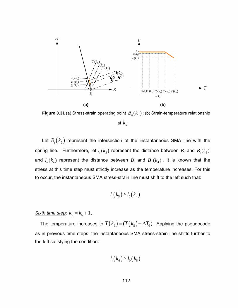
112
ε
σ
iB
5( )tB k4( )oB k
5(
)tl k
4(
)ol k
5( )oB k
1( )T k4( )T k
5( )T k
T
ε
pε
( )oT k 3( )
f
T kT=
1( )T k 4( )T k
4( )kε
5( )T k
5( )kε
(a) (b)
Figure 3.31 (a) Stress-strain operating point 5( )oB k ; (b) Strain-temperature relationship
at 5k
Let ( )5tB k represent the intersection of the instantaneous SMA line with the
spring line. Furthermore, let 5( )tl k represent the distance between iB and 5( )tB k
and 4( )ol k represent the distance between iB and 4( )oB k . It is known that the
stress at this time step must strictly increase as the temperature increases. For this
to occur, the instantaneous SMA stress-strain line must shift to the left such that:
( ) ( )5 0 4tl k l k≥
Sixth time step: 6 5 1k k= + ,
The temperature increases to ( ) ( )6 5 6( )T k T k T= +Δ . Applying the pseudocode
as in previous time steps, the instantaneous SMA stress-strain line shifts further to
the left satisfying the condition:
( ) ( )6 0 5tl k l k≥

113
The graphical representation of the equations and operating point for time step
6k are shown in Figure 3.32a. The actuation output of the system up to 6k is shown
in Figure 3.32b.
ε
σ
iB
6( )oB k1( )T k
6( )T k
4( )T k5( )T k
T
ε
pε
( )oT k3( )
f
T kT=
1( )T k 4( )T k
4( )kε
5( )T k
5( )kε
6( )T k
6( )kε
(a) (b)
Figure 3.32 (a) Stress-strain operating point ( )6oB k ; (b) Strain-temperature relationship
at 6k
The above modeling scheme can be continued until the time step nk when
( ) ( )( )1n n n eT k T k T T−= +Δ = . The evolution of the solution through time is shown in
Figure 3.33.

114
ε
σ
K
iB
1( )T k
6( )T k
4( )T k5( )T k
( )nT k
( )o nB k
T
ε
pε
( )oT k 3( )
f
T kT=
1( )T k 4( )T k
4( )kε
5( )T k
5( )kε
6( )T k ( )nT k
6( )kε
( )nkε
(a) (b) Figure 3.33 Time evolution of a stable simulation: (a) stress-strain plot and (b) actuation
output
Figure 3.34 shows actual MATLAB simulation results using the aforementioned
pseudocode. The parameters chosen for this simulation are 27.7fT = , 71.1 10fa = ⋅ ,
82.21 10Mσ += ⋅ , 83.7 10σΔ = ⋅ and 108 10K = ⋅ .
(a) (b) Figure 3.34 MATLAB simulation of explicit modeling scheme: (a) Stress-strain plot and
(b) actuation output

115
Although this explicit approach is straightforward, it suffers from convergence
issues associated with the magnitude of K and the sampling frequency. An
important assumption made in the explicit modeling scheme is that the
instantaneous SMA stress-strain line shifts to the left at every time step such that:
( ) ( )0 1t n nl k l k −≥ when
( ) ( )1n nT k T k −≥ (3.38)
Conversely, when the temperature decreases, the instantaneous SMA stress-
strain line is assumed to shift to the right such that:
( ) ( )0 1t n nl k l k −< when
( ) ( )1n nT k T k −< (3.39)
However, these conditions are difficult to guarantee when the value of K is
small. For such cases, the modeling scheme results in an unstable simulation. To
understand this instability, a second simulation of the pseudocode, this time for
much lower spring stiffness, will be described.
Consider again the system consisting of a spring connected to a SMA actuator
represented by a single SCSMA element. The parameters for the strain-based
neuron representing the SCSMA are same as before and the temperature is set to
increase monotonically from ( )0 aT k T= (ambient temperature) to ( )n eT k T= . For
brevity, the simulation up to time step 4k is omitted as the pseudocode behavior is
the same as that for the stable case. The graphical representation of the equations

116
and the operating point at time step 4k are shown in Figure 3.35a. The actuation
output of the system up to 4k is shown in Figure 3.35b.
ε
σ
iB
K
1( )T k4( )T k
4( )kσ
4( )kε
4( )oB k
T
ε
pε
( )oT k 3( )
f
T kT=
1( )T k 4( )T k
4( )kε
(a) (b)
Figure 3.35 (a) Stress-strain operating point 4( )oB k ; (b) Strain-temperature relationship
at 4k
Fifth time step: 5 4 1k k= + ,
The temperature increases to ( ) ( )5 4 5( )T k T k T= +Δ . Applying the pseudocode
as described for the stable case, the instantaneous SMA stress-strain line shifts
further to the left. However, since the spring stiffness is very low, the strain
increment due to the spring model at time step 4k is relatively large. Consequently,
the shift in the instantaneous SMA line is not sufficient to satisfy the condition
( ) ( )5 0 4tl k l k≥ . Consequently the stress calculated at time step 5k ( )5kσ( ) is lower
than the previous time step. The operating point ( )5oB k and the equations of SMA
and spring are represented in Figure 3.36a. The actuation output of the system up to
5k is shown in Figure 3.36b.

117
ε
σ
iB
5(
)tl k
4(
)ol k
5( )tB k4( )oB k
5( )oB k
1( )T k4( )T k
5( )T k
T
ε
pε
( )oT k 3( )
f
T kT=
1( )T k 4( )T k
4( )kε
5( )T k
(a) (b)
Figure 3.36 (a) Stress-strain operating point 5( )oB k ; (b) Strain-temperature relationship
at 5k
Sixth time step: 6 5 1k k= + ,
The temperature increases to ( ) ( )6 5 6( )T k T k T= +Δ . Applying the pseudocode
in the same fashion as previous time step, the instantaneous SMA stress-strain line
shifts further to the left. However, the condition ( ) ( )6 0 5tl k l k≥ is satisfied at this
time step and consequently the stress increases. The graphical representation of the
equations and operating point are shown in Figure 3.37a and the actuation output of
the system up to 6k is shown in Figure 3.37b.

118
ε
σ
1( )T k
6( )T k
4( )T k5( )T k
6( )oB k
iB
T
ε
pε
( )oT k 3( )
f
T kT=
1( )T k 4( )T k
4( )kε
5( )T k 6( )T k
6( )kε
(a) (b)
Figure 3.37 (a) Stress-strain operating point 6( )oB k ; (b) Strain-temperature relationship
at 6k
Continuing the modeling scheme for successive time steps, the unstable
evolution of the simulation can be observed as shown in Figure 3.38. It can be
inferred that the onset of instability occurs when the stability conditions (3.38) and
(3.39) are not satisfied at any time step.

119
ε
σ
K 1( )T k
6( )T k
4( )T k5( )T k
( )nT k
iBT
ε
pε
( )oT k 3( )
f
T kT=
1( )T k 4( )T k
4( )kε
5( )T k 6( )T k
6( )kε
( )nT k
(a) (b)
Figure 3.38 Time evolution of an unstable simulation: (a) stress-strain plot and (b)
actuation output
Figure 3.39 shows MATLAB simulation results for the SMA-spring system with a
lower actuator modulus ( 3.4 10K e= ). The parameters for the strain-based neuron
are the same as those for the stable case. The unstable evolution of the simulation
through time can be observed in these figures.
(a) (b)
Figure 3.39 Stress-strain plot (a) and actuation output (b) of an unstable simulation in
MATLAB

120
It is clear that explicit modeling scheme is not reliable method of modeling the
SMA-spring system because of the need to guarantee that conditions (3.38) and
(3.39) are satisfied at all times. Difficulties in satisfying these stability conditions are
further exacerbated when the SMA actuator is modeled with a HRNN consisting of
numerous SCSMA elements.
3.7.2 Implicit modeling scheme
To overcome these convergence issues, an implicit method is needed such that
the operating point ( ) ( )( ),tB k kε σ can be identified at every time step; it can then
be incremented to satisfy the condition ( ) ( )o tl k l k= . In other words, the stress and
strain at each time step can be obtained by solving the instantaneous SMA
equations and the spring equation. This is easily achieved for the simple case of a
spring actuated by a single SCSMA element. For a SCSMA element represented by
a strain-based neuron, the stress and strain are obtained by solving (3.33) and
(3.37) giving:
( )
( )1 1
( )
p T Mx kk
Eeff k K
ε εσ +
−=⎛ ⎞
+⎜ ⎟⎝ ⎠
(3.40)
and:
( )
( )( )1
( )
p T MK x k
Eeff kkK
Eeff k
ε εε
++
=⎛ ⎞+⎜ ⎟
⎝ ⎠
(3.41)

121
It can be seen that the stress and strain at every time step are calculated
independently and have no direct dependencies on stress and strain from previous
iteration. Hence the relation between stress and strain is ‘implicit’. The implicit
modeling procedure is depicted in the block diagram of Figure 3.40.
( )kσ( )T k
( )kε
Figure 3.40 Block diagram for implicit modeling scheme
The extension of this implicit modeling scheme to a polycrystalline SMA-spring
system involves the determination of stresses and strains associated with multiple
SCSMA elements. Specifically, the instantaneous equation of the SMA actuator is a
weighted combination of equations for each SCSMA element. For each strain-based
neuron:
( ) ( ) ( )( ),( ) ( )i i T M ik Eeff k k k x kσ ε ε+
= − (3.42)
Multiplying both sides by 2iw and summing over all the neurons gives:
( ) ( )( ) ( )2 2,
1 1( ) ( )
N N
i i T M i i ii i
k w k k x k Eeff k wσ ε ε+
= =
= −∑ ∑ (3.43)
But for the HRNN composed of these strain-based neurons:
( ) 2
1( )
N
i ii
k k wσ σ=
=∑ (3.44)

122
Hence, the instantaneous stress-strain equation of the SMA actuator is given by:
( ) ( ) ( )( ) ( )2 2,
1 1( ) ( )
N N
i i T M i i ii i
k k Eeff k w k x k Eeff k wσ ε ε+
= =
= −∑ ∑ (3.45)
The spring equation is:
( ) ( )p
kk
Kσ
ε ε= − (3.46)
Substituting (3.46) in (3.45) and rearranging the terms, the stress on the SMA
actuator is:
( )( ) ( )
( )
2,
12
1
( )1
N
p T M i i ii
Ni i
i
x k Eeff k wk
Eeff k wK
ε εσ
+=
=
−=
+
∑
∑ (3.47)
The strain on the SMA ( ( )kε , which is equal for all neurons) and the stress
associated with each strain-based neuron can then be obtained using the value of
( )kσ . The pseudocode for implementing the implicit modeling scheme for a SMA-
spring system is as follows:
1) For each strain-based neuron in the HRNN
a. Calculate the output of the difference equations for the current time
step k
b. Calculate the accumulative terms in (3.47) which are:

123
i. ( ) ( )( ) ( ) 2,i p T M i i iNr k x k Eeff k wε ε
+= −
ii. ( ) ( ) 2i i
i
Eeff k wDr k
K=
2) Sum the accumulative terms over all the neurons and use the results to
determine ( )kσ from (3.47):
1
1
( )( )
1 ( )
N
ii
N
ii
Nr kk
Dr kσ =
=
=+
∑
∑ (3.48)
3) Determine ( )kε by substituting ( )kσ into (3.46)
4) For each strain-based neuron in the HRNN
a. Calculate ( )i kσ by substituting ( )kε into (3.42)
5) Move to the next time step ( 1k k= + ) and repeat steps 1-4
Figure 3.41 shows a simulation of quasi-static actuation of a SMA-spring system
with the SMA modeled by a HRNN consisting of 30 strain-based neurons. For this
simulation, all neuron weights are initialized equally ( 0.1826iw = ).

124
(a) (b)
(c)
Figure 3.41 (a) Simulated actuation response of SMA actuator and (b) simulated strain-
strain behavior of two of the neurons in the HRNN for temperature input (c)
The implicit modeling scheme developed in this section is found to be very robust
with respect to actuator modulus and time step. Consequently, this solution scheme
is extended to a system with antagonistic SMA tendons which is central to modeling
of the robotic catheter.

125
3.8 Modeling planar catheter actuation with antagonistic SMA tendons
A shortcoming of the SMA-spring system (Figure 3.27) presented in the last
section is that its actuation bandwidth is limited. Although the SMA can be heated
rapidly, its cooling is governed by conductive and convective heat transfer modes
which are relatively slow. Hence the bandwidth of the system is limited by the
cooling rates of the system. However, the bandwidth can be greatly improved using
dual SMA actuators in antagonistic configuration. In this configuration, the cooling
phase of any one actuator is not a limiting factor since its antagonistic counterpart
can be in heated in order to improve the response. Consequently, the catheter is
also designed on this principle.
As explained previously (Chapter 2, Section 2.8), the catheter dynamics can be
decoupled into two orthogonal planes. Furthermore, the decoupled dynamics can be
modeled as a central tube actuated by two antagonistic SMA tendons; this simplified
model is called a Planar Catheter Bending (PCB) system. This section extends the
implicit modeling scheme to model such a PCB system. The two polycrystalline SMA
tendons in the PCB system can be represented as a series combination or a parallel
combination of SCSMA elements. The implicit modeling scheme is developed for
each of these representations and their advantages and disadvantages are
discussed. Additional nonlinear effects, including the occurrence of slack in the
tendons, are also taken into consideration.
3.8.1 Parallel combination of SCSMA elements
In this representation, each SMA tendon (designated as xz+ and xz− tendons)
is represented by a parallel combination of SCSMA elements. Also, the implicit
modeling scheme derived for a single SMA actuator in Section 3.7 is extended to the
PCB system by using two HRNNs composed of strain-based neurons to represent
the two tendons. Figure 3.42a illustrates this approach of modeling each SMA

126
tendon and Figure 3.42b shows an equivalent representation of the catheter in terms
of a spring and parallel SCSMA elements.
(a) (b)
Figure 3.42. (a) SMA tendons represented as parallel combination of SCSMA elements
and (b) Equivalent representation in terms of spring and parallel SCSMA elements
From (2.43), tube bending in the xz plane can be described:
( )xz xz
xz ptubeK
σ σε ε + −+
−= − (3.49)
where xzε + is the strain of the ‘ xz+ ’ tendon, xzσ + , xzσ − are the stresses on the
two tendons and pε is the prestrain on each tendon. The equivalent stiffness of the
tube is given by:
2tubeEIK
a A= (3.50)

127
Also:
p xz xz pε ε ε ε+ −− = − (3.51)
Therefore, (3.49) can also be written as:
( )xz xz
xz ptubeK
σ σε ε + −−
−= + (3.52)
For the HRNN representing the xz+ tendon (HRNN+xz):
( ) 2, ,
1( )
xzN
xz xz i xz ii
k k wσ σ+
+ + +=
= ∑ (3.53)
where xzN+ is the number of neurons in HRNN+xz, ( ),xz i kσ+ is the output stress
of the ith neuron and ,xz iw+ is its associated weight.
Also for the ith neuron in HRNN+xz:
( ) ( )( ) ( ), , , ,( )xz i xz T xz M i xz ik k x k Eeff kσ ε ε++ + + += − (3.54)
Similarly, for HRNN-xz:
( ) 2, ,
1( )
xzN
xz xz i xz ii
k k wσ σ−
− − −=
= ∑ (3.55)

128
and:
( ) ( )( ) ( ), , , ,( )xz i xz T xz M i xz ik k x k Eeff kσ ε ε+− − − −= − (3.56)
Multiplying both sides of (3.54) by ,
2xz i
w+
and summing over all neurons in the
HRNN+xz, gives:
( )( ) ( ) 2, , , ,
1( ) ( ) ( )
xzN
xz xz T xz M i xz i xz ii
k k k x k Eeff k wσ ε ε+
++ + + + +=
= −∑ (3.57)
Substituting (3.49) in (3.57) and rearranging the terms:
( ) ( )
( )( ) ( )
2 2, , , ,
1 1
2, , , ,
1
( ) 1 ( )
xz xz
xz
N Nxz i xz i xz i xz i
xz xzi itube tube
N
p T xz M i xz i xz ii
Eeff k w Eeff k wk k
K K
x k Eeff k w
σ σ
ε ε
+ +
+
+
+ + + ++ −
= =
+ + +=
⎛ ⎞ ⎛ ⎞+ + −⎜ ⎟ ⎜ ⎟
⎝ ⎠ ⎝ ⎠
= −
∑ ∑
∑(3.58)
Similarly for HRNN-xz:
( ) ( )
( )( ) ( )
2 2, , , ,
1 1
2, , , ,
1
( ) ( ) 1
xz xz
xz
N Nxz i xz i xz i xz i
xz xzi itube tube
N
p T xz M i xz i xz ii
Eeff k w Eeff k wk k
K K
x k Eeff k w
σ σ
ε ε
− −
−
+
− − − −+ −
= =
− − −=
⎛ ⎞ ⎛ ⎞− + +⎜ ⎟ ⎜ ⎟⎝ ⎠ ⎝ ⎠
= −
∑ ∑
∑(3.59)
( )xz kσ + and ( )xz kσ − at each time step can be obtained by solving between the two
linear equations (3.58) and (3.59). The strains on individual tendons as well as the

129
stresses associated with each strain-based neuron in both HRNNs can then be
obtained from the value of these stresses. The associated pseudocode to implement
the implicit modeling scheme is as follows:
1) For each strain-based neuron in the HRNN+xz
a. Calculate the output of the difference equations for the current time
step k
b. Calculate the accumulative terms in (3.58) which are:
i. ( ) 2
, ,1, ( ) xz i xz i
itube
Eeff k wa k
K+ +=
ii. ( ) ( )( ) ( ) 21, , , , ,i p T xz M i xz i xz ib k x k Eeff k wε ε
++ + += −
2) For each strain-based neuron in the HRNN-xz
a. Calculate the output of the difference equations for the current time
step k
b. Calculate the accumulative terms in (3.59) which are:
i. ( ) 2
, ,2, ( ) xz i xz i
itube
Eeff k wa k
K− −=
ii. ( ) ( )( ) ( ) 22, , , , ,i p T xz M i xz i xz ib k x k Eeff k wε ε
+− − −= −
3) Construct two simultaneous linear equations from the accumulated terms as
follows:
11 12 1( ) ( ) ( ) ( ) ( )xz xzk A k k A k B kσ σ+ −+ = (3.60)

130
21 22 2( ) ( ) ( ) ( ) ( )xz xzk A k k A k B kσ σ+ −+ = (3.61)
where
11 1,1
( ) 1 ( )xzN
ii
A k a k+
=
= + ∑ , 12 1,1
( ) ( )xzN
ii
A k a k+
=
= −∑ , 1 1,1
( ) ( )xzN
ii
B k b k+
=
= ∑
21 2,1
( ) ( )xzN
ii
A k a k−
=
= −∑ , 22 2,1
( ) 1 ( )xzN
ii
A k a k−
=
= + ∑ , 2 2,1
( ) ( )xzN
ii
B k b k−
=
= ∑
4) Solve between Equations (3.60) and (3.61) to obtain ( )xz kσ + and ( )xz kσ −
5) Calculate ( )xz kε + and ( )xz kε − by substituting ( )xz kσ + and ( )xz kσ − into
Equations (3.49) and (3.52) respectively.
6) For each strain-based neuron in the HRNN+xz
a. Calculate ( ),xz i kσ+ by substituting ( )xz kε + into (3.54)
b. If ( ), 0xz i kσ+ < (occurrence of slack in the SCSMA element
represented by the ith neuron of HRNN+xz) then set ( ), 0xz i kσ+ =
7) For each strain-based neuron in the HRNN-xz
a. Calculate ( ),xz i kσ− by substituting ( )xz kε − into (3.56)
b. If ( ), 0xz i kσ− < (occurrence of slack in the SCSMA element
represented by the ith neuron of HRNN-xz) then set ( ), 0xz i kσ− =
8) Move to the next time step ( 1k k= + ) and repeat steps 1-7
In the above pseudocode, whenever slack is detected in any SCSMA element, its
associated stress is set to 0. The strain associated with such a SCSMA element will
not be equal to the strain of the tendon until all the slack is recovered by heating the

131
tendon. Figure 3.43a shows a simulation of a PCB system with each tendon of the
PCB system alternately actuated as per input temperature profile in Figure 3.43b.
Here, each HRNN is composed of 100 strain-based neurons with all neuron weights
set equal.
(a) (b)
Figure 3.43 Actuation of PCB system: (a) tendon strains (b) temperature applied to
individual tendons
It is evident from the above simulations that the implicit modeling scheme for the
PCB system results in a stable simulation. However, one shortcoming of
representing each SMA tendon as a parallel combination of SCSMA elements is the
need for very high sampling rates (>7 samples/sec). This is because changes in
stress associated with each strain-based neuron are functions of tendon strain
(Steps 6 and 7 of pseudocode for implicit modeling scheme). Sometimes, even small
changes in tendon strain can cause large changes in stresses in some of the
individual neurons. The difference equations of strain-based neurons are very
sensitive to such large changes in stresses. Hence, to ensure that the strain
changes associated with the tendon are not excessively large at any time step, the
sampling interval needs to be reduced dramatically. This is especially undesirable
when the HRNNs need to be used in real-time control algorithms. However, the

132
representation of SMA tendons as a series combination of SCSMA elements stands
as a solution to this problem.
3.8.2 Series combination of SCSMA elements
Figure 3.44 illustrates this modeling approach in terms of a spring and a series
SCSMA elements.
(a) (b)
Figure 3.44. SMA tendons represented as a series combination of SCSMA elements
The procedure to derive the implicit modeling scheme for the series
representation is similar to the parallel representation except the roles of stresses
and strains are switched. As before, two HRNNs are needed to represent the two
tendons.
For HRNN+xz:

133
( ) 2, ,
1( )
xzN
xz xz i xz ii
k k wε ε+
+ + +=
= ∑ (3.62)
where for the ith neuron in the HRNN+xz:
( ) ( )
( ) ( )/
, , ,
, , , ,
( )
( ) ( )
xzxz i T xz M i
M
xz xzxz A i xz M i
A M
kk x kE
k kx k x kE E
σε ε
σ σ
+
+ −
++ +
+ ++ +
⎛ ⎞= +⎜ ⎟⎝ ⎠
⎛ ⎞ ⎛ ⎞+ +⎜ ⎟ ⎜ ⎟⎝ ⎠ ⎝ ⎠
(3.63)
After rearranging, (3.63) can be written as:
( ) ( )( ) ( ), , ,
,
xzxz i T xz M i
xz i
kk x k
Eeff kσ
ε ε+
++ +
+
= + (3.64)
Similarly, for the HRNN-xz:
( ) ( ) 2, ,
1
xzN
xz xz i xz ii
k k wε ε−
− − −=
= ∑ (3.65)
and:
( ) ( ) ( ), , ,,
( )xzxz i T xz M i
xz i
kk x kEeff kσε ε
+
−− −
−
= + (3.66)
Multiplying both sides of (3.64) by ,
2xz i
w+
and summing over all neurons in the
HRNN+xz, gives:

134
( ) ( ) ( ),
,
22
, ,1 1,
( )xz xz
xz i
xz i
N N
xz xz T xz M ii ixz i
wk k x k w
Eeff kε σ ε
+ ++
+ ++ + += =+
= +∑ ∑ (3.67)
Substituting (3.49) in (3.57) and rearranging the terms:
( ) ( ) ( )
( )
,
,
2
1 ,
2, ,
1
1 1
xzxz i
xz
xz i
N
xz xzi xz i tube tube
N
p T xz M ii
wk k
Eeff k K K
x k w
σ σ
ε ε
++
+
+ +
+ −= +
+=
⎛ ⎞⎛ ⎞ ⎛ ⎞⎜ ⎟+ + −⎜ ⎟ ⎜ ⎟⎜ ⎟⎜ ⎟ ⎝ ⎠⎝ ⎠⎝ ⎠
= −
∑
∑ (3.68)
Similarly for HRNN-xz:
( ) ( ) ( )
( )
,
,
2
1 ,
2, ,
1
1 1
xzxz i
xz
xz i
N
xz xzitube xz i tube
N
p T xz M ii
wk k
K Eeff k K
x k w
σ σ
ε ε
−−
−
+ −
+ −= −
−=
⎛ ⎞⎛ ⎞⎛ ⎞⎜ ⎟− + +⎜ ⎟⎜ ⎟ ⎜ ⎟⎜ ⎟⎝ ⎠ ⎝ ⎠⎝ ⎠
= −
∑
∑ (3.69)
( )xz kσ + and ( )xz kσ − at each time step can be obtained by solving between the
two linear equations (3.68) and (3.69). The associated pseudocode to implement the
implicit modeling scheme for the series representation is as follows:
1) For each strain-based neuron in the HRNN+xz
a. Calculate the output of the difference equations for the current time
step k
b. Calculate the accumulative terms in (3.68) which are:

135
i. ( )
,
2
1,,
( ) xz i
ixz i
wa k
Eeff k+
+
=
ii. ( ) ( ),
21, , , xz ii T xz M ib k x k wε
+ ++=
2) For each strain-based neuron in the HRNN-xz
a. Calculate the output of the difference equations for the current time
step k
b. Calculate the accumulative terms in (3.69) which are:
i. ( )
,
2
2,,
( ) xz i
ixz i
wa k
Eeff k−
−
=
ii. ( ) ( ),
22, , , xz ii T xz M ib k x k wε
+ −−=
3) Construct two simultaneous linear equations from the accumulated terms as
follows:
11 12 1( ) ( ) ( ) ( ) ( )xz xzk A k k A k B kσ σ+ −+ = (3.70)
21 22 2( ) ( ) ( ) ( ) ( )xz xzk A k k A k B kσ σ+ −+ = (3.71)
where

136
11 1,1
1( ) ( )xzN
ii tube
A k a kK
+
=
= +∑ , 121( )tube
A kK
= − , 1 1,1
( ) ( )xzN
p ii
B k b kε+
=
= − ∑
211( )tube
A kK
= − , 22 2,1
1( ) ( )xzN
ii tube
A k a kK
−
=
= +∑ , 2 2,1
( ) ( )xzN
p ii
B k b kε−
=
= −∑
4) Solve between Equations (3.70) and (3.71) to obtain ( )xz kσ + and ( )xz kσ −
5) For HRNN+xz, if ( ) 0xz kσ + < (occurrence of slack in the ‘ xz+ ’ tendon) then
set ( ) 0xz kσ + =
6) For HRNN-xz, if ( ) 0xz kσ − < (occurrence of slack in the ‘ xz− ’ tendon) then
set ( ) 0xz kσ − =
7) Move to the next time step ( 1k k= + ) and repeat steps 1-7
Comparing this pseudocode to that for the parallel representation, it can be seen
that the number of steps is reduced. The stress calculated for each tendon equals
the stress associated with every stress-based SCSMA element representing that
tendon. Hence, the stress can directly be applied to the next time step, unlike the
parallel representation where the stresses on individual elements needed to be
calculated after the computation of tendon stresses. This leads to additional
reductions in computational cost.
Sampling rate requirements can be greatly relaxed in the series representation to
as low as 1 sample/sec of quasi-static data compared to the 7 samples/sec required
for parallel representations. This is because changes in stress are relatively small,
even when the sampling interval is relatively long.

137
The relaxed sampling rate requirements and higher computational efficiencies
make the implicit modeling scheme for the series representation more suitable for
modeling the PCB system. Consequently, this solution scheme will be the modeling
technique of choice for training the HRNN using experimental data.
3.8.3 Training HRNNs for the PCB system
From the discussions of the previous sections, it is evident that the most suitable
technique to model the PCB system is to use the implicit scheme with a series
representation of the SMA tendons. Individual HRNNs can then be trained on the
experimental data collected by actuating the PCB system. Data from the PCB
system was obtained using the dual-camera measurement system described in
Chapter 2. The PCB system was actuated quasi-statically using slowly varying PWM
duty cycles. Since the data is collected under quasi-static conditions, the relation
between the PWM duty cycle and the temperature in each tendon can be assumed
to be algebraic given by the steady state solution of the heat transfer model (2.22)
presented in Chapter 2. The relation can hence be derived as:
( ) ( )T k cu k= (3.72)
where ( )T k is the temperature, ( )u k is the PWM duty cycle and c is a constant
derived from (2.22) as:
( )1 2 maxc g g j= + (3.73)
Data was first collected by actuating the xz+ tendon of the PCB system from its
neutral position (0° bending angle) using the using a sequence of input PWM duty
cycles shown in Figure 3.45a. The catheter was then reset to the neutral position
and data is then collected by actuating xz− tendon using the same sequence of

138
PWM duty cycles as that for the xz+ tendon. The resulting experimental responses
are shown in Figure 3.45b. Test data was also collected using the continuous
sequence of PWM duty cycles shown in Figure 3.46a. The resulting experimental
responses are shown in Figure 3.46b.
(a) (b) Figure 3.45 Experimental training data obtained from the PCB system: (a) input and (b)
output
(a) (b)
Figure 3.46 Experimental test data obtained from the PCB system: (a) input and (b)
output

139
In order to model the PCB system using the implicit scheme, two HRNNs
representing the two tendons were each initialized with 400 neurons. The four
parameters for each neuron were initialized with random values across the following
ranges: [ ], 20,30f iT ∈ , 6 7, 3 10 , 2 10f ia ⎡ ⎤∈ ⋅ ⋅⎣ ⎦ , 7 8
, 2 10 , 2.75 10M iσ+
⎡ ⎤∈ ⋅ ⋅⎣ ⎦ and
7 85 10 ,6 10iσ ⎡ ⎤Δ ∈ ⋅ ⋅⎣ ⎦ . In addition to these neurons, two neurons were added to each
HRNN with their parameters set such that they always stay either in the M + phase
or the A phase and their weights were set constant. Since the experimental data
only represents the transformations specific to the system, it does not capture the
effects of crystals that do not participate in actuation. The purpose of the two non-
transforming neurons is to account for all such crystals.
The implicit modeling scheme was implemented and after every time step the
bending angle predicted by the model was compared against the experimental
training data to generate error. This error was used in conjunction with a Levenberg-
Marquardt algorithm to train the two HRNNs. The HRNNs were trained for 18
epochs and the weights of neurons in each HRNN were normalized after each
epoch. The result of the training is presented in Figure 3.47a. For clarity, the training
data from actuation each tendon with respect to time are shown in comparison with
the HRNN predictions in Figure 3.47b and Figure 3.47c. The performance of the
trained HRNN model on test data (not included in the training process) is shown in
Figure 3.48. These results clearly demonstrate the modeling accuracy of the HRNN
model for the PCB system.

140
(a)
(b) (c)
Figure 3.47 Comparison of experimental training data and HRNN predictions

141
Figure 3.48 Comparison of experimental test data with HRNN predictions

142
Chapter 4. Control of the Robotic Catheter
4.1 Introduction
With increasing interest in shape memory alloys and their applications, there has
been significant research into developing control algorithms for SMA actuated
systems. As explained in previous chapters, the hysteresis in SMA is an important
phenomenon which must be addressed during control synthesis. Past research on
model-based control of SMA actuated structures has focused primarily on models
which are either computationally intensive (and cannot run in real-time) or inaccurate
for polycrystalline materials. Furthermore, much of the published research utilizes
single-input, single-output strategies that cannot be readily extended to multiple
antagonistic actuators.
Numerous control algorithms that have been developed for SMA-spring systems
like the one described in Chapter 3. A proportional controller was implemented and
analyzed by Da Silva to control the deflection of a flexible beam [64]. Jayender, et.
al, demonstrated the performance of a gain-scheduled proportional-integral (PI)
controller and a robust controller, both based on a linearized model similar to
Tanaka [62]. Ashrafiuon, et al. proposed a variable structure controller that was
applied to 3-link SMA actuated robot. Seelecke and Muller [39] proposed an optimal
control technique to increase actuation bandwidth while optimizing the input power
with applications to MEMS-based devices. Although this method could potentially be
adapted for catheter actuation, it requires a priori knowledge of the tip trajectory,
making it unsuitable for real-time tracking control. Intelligent controllers based on
neural networks (NN) are well suited to this multivariable SMA actuation application
because they can potentially capture the dynamics of the catheter using measured
input-output data. Song, et. al incorporated an inverse neural network with a sliding
mode controller (SMC) and demonstrated its application to a SMA wire [53]. Neural
networks have also been used to model the relationship between the electrical

143
resistance and strain of an SMA wire. Such a network coupled with a proportional-
derivative (PD) controller eliminates the need for position sensors [65]. However, in
all these cases the neural network was only trained on the outer loop of the
hysteresis, and therefore would inhibit tracking that includes numerous inner loop
reversals.
This chapter demonstrates the use of HRNNs in developing real-time controllers
for SMA-actuated catheters. As demonstrated in the previous chapter, the HRNN
has the capability to accurately model the polycrystalline nature of the material and
capture its inner loop behavior. Furthermore, the HRNN was demonstrated to
accurately model a decoupled single-segment catheter system (Chapter 3, Section
3.8). An HRNN-based controller has the potential to provide excellent tracking
performance while optimizing input power, thus enabling operation at lower
temperatures. This is especially important as high temperatures can adversely affect
tissues that come in contact with the catheter. Motivated by these reasons, a control
algorithm based on the HRNN is developed for a PCB system. Two of these
controllers implemented for PCB systems in each orthogonal direction can then be
used to control a single-segment catheter. Due to current limitations on hardware,
the HRNN-based control is demonstrated through simulations rather than on the
actual system. However, PI and PID controllers are implemented on the actual
system to demonstrate the speed and accuracy that can be achieved in the catheter
system.
4.2 Control system setup
It was shown in Chapter 2 (Section 2.7) that the dynamics of the catheter can be
decoupled into two orthogonal directions where the bending angles in each
orthogonal plane are given by:
( )sinxzθ θ ϕ= (4.1)

144
( )cosyzθ θ ϕ= (4.2)
This decoupled representation was termed a planar catheter bending (PCB)
model in Chapter 2. The tracking errors between the reference angles and
measured angles can be expressed:
( ) ( )sin sinxz ref refe θ ϕ θ ϕ= − (4.3)
( ) ( )cos cosyz ref refe θ ϕ θ ϕ= − (4.4)
where refθ and refϕ are the reference bending and orientation angles of the catheter,
respectively. As a result of this decoupling, two separate controllers can be used to
control the bending angle of the PCB system in each orthogonal plane (Figure 4.1).
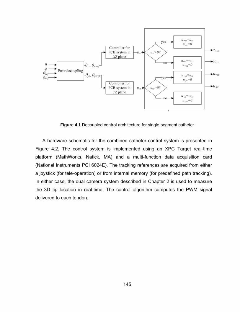
145
Figure 4.1 Decoupled control architecture for single-segment catheter
A hardware schematic for the combined catheter control system is presented in
Figure 4.2. The control system is implemented using an XPC Target real-time
platform (MathWorks, Natick, MA) and a multi-function data acquisition card
(National Instruments PCI 6024E). The tracking references are acquired from either
a joystick (for tele-operation) or from internal memory (for predefined path tracking).
In either case, the dual camera system described in Chapter 2 is used to measure
the 3D tip location in real-time. The control algorithm computes the PWM signal
delivered to each tendon.

146
Figure 4.2 Schematic of the single-segment catheter control system
4.3 HRNN based control of PCB system
A feed-forward controller-based on the HRNN model is developed for controlling
the bending angle of a PCB system. This control scheme essentially involves
inverting the HRNN model so that the reference bending angle is its input and the
PWM duty cycles for each tendon are outputs. A direct inversion of the HRNN
model is not possible given its complexity and non-linear characteristics. Hence, an
algorithm is developed to approximate the pseudoinverse of an HRNN model.
The block diagram of the HRNN-based feed-forward controller is shown in
Figure 4.3. For clarity, the PCB system is considered to operate in the XZ plane and
the subscripts xz+ , xz− are used to denote parameters associated with the xz+tendon and xz− tendon respectively (Chapter 2, Section 2.8). This controller is
composed of two parts. The first part is the HRNN model (G ) for the PCB system.

147
Its inputs include the estimated temperatures of each tendon ( ( )xzT k+ , ( )xzT k− ), the
neuron states from the previous time step ( ( )( ), 1..1
xzM i i Nf k
++ =− , ( )( ), 1..
1xzA i i N
f k+ =
− ,
( )( ), 1..1
xzM i i Nf k
−+ =− , ( )( ), 1..
1xzA i i N
f k− =
− ) and the tendon stresses from the previous
time step ( ( )1xz kσ+ − , ( )1xz kσ− − ). The neuron states and tendon stresses at the
present time step are computed using G and the implicit modeling scheme
discussed in Chapter 3. G also provides estimates of the catheter bending angle
( )NN kθ for the present time step and hence functions like an observer.
Figure 4.3 HRNN based feed-forward controller for a PCB system
148
Inputs to the pseudoinverse model 1G− include the reference bending angle
( )ref kθ and the estimated bending angle at the present time step. Other
inputs include the estimated temperatures and , the neuron states
( )( ), 1..xzM i i Nf k
++ =, ( )( ), 1..xzA i i N
f k+ =
, ( )( ), 1..xzM i i Nf k
−+ =, ( )( ), 1..xzA i i N
f k− =
and the
stresses associated with each tendon ( )xz kσ + and ( )xz kσ − . The pseudoinverse
algorithm essentially integrates forward in time to determine the control input
necessary to drive the PCB system to the reference bending angle. The algorithm to
compute the pseudoinverse is outlined in flowchart of Figure 4.4. Since the
pseudoinverse algorithm integrates forward in time at each time step, the variables
local to this algorithm and are marked by a line above them ( X ) to distinguish them
from their real-time counterparts ( X ).
( )NN kθ
( )xzT k+ ( )xzT k−

149
Figure 4.4 Algorithm for computing the pseudoinverse
The pseudoinverse algorithm first determines if the estimated bending angle is
within tolerance limits ( 0.5tolθ = ° ) of the reference angle; if so then the reference
tendon temperatures are set to the present estimated tendon temperatures. These
tolerance limits establish a controller “dead zone” that helps prevent chatter in the

150
output response. The corresponding PWM duty cycles are computed to maintain
these tendon temperatures. Steady state relationships between PWM duty cycle and
tendon temperature are determined by applying the final value theorem to the heat
transfer model (2.22); for the thi tendon:
i iu cT= (4.5)
where c is a constant determined from equation (2.22) as:
( )1 2 maxc g g j= + (4.6)
If the estimated bending angle is outside the tolerance limits of the reference
bending angle, the pseudoinverse algorithm determines which tendon needs to be
actuated based on whether is greater than or less than . For
example, if ( ) ( )ref NNk kθ θ> then the xz+ tendon must be activated to increase its
temperature while the xz− must be deactivated. Once the active tendon is
determined, the temperature response of the deactivated is simulated using the
inverse Laplace transform of the heat transfer model (2.22). This temperature profile,
which monotonically decreases from its present estimated value (e.g. ( )xzT k− ), is
simulated for a sufficiently long time horizon of 100s. The active tendon temperature
is then incremented for each time step k until the estimated bending angle of the
pseudoinverse algorithm ( )NN kθ is equal to ( )ref kθ . The resulting active tendon
temperature that satisfies this condition is designated the feed-forward temperature
(e.g. ( )xzffT k+ ). The active tendon PWM duty cycle is computed to reach the feed-
forward temperature as quickly as possible:
( )ref kθ ( )NN kθ

151
( ) ( )active ss Temp Tempu k u k K e= + (4.7)
where Tempe is the difference between the feed-forward temperature and the current
estimated temperature of the tendon and TempK is a proportional gain. ( )ssu k is the
PWM input needed to achieve the steady state feed-forward temperature and
determined as before, by applying the final value theorem to the heat transfer model
(2.22).
4.4 Simulated control results
To evaluate the effectiveness of this feed-forward control strategy, simulations
were conducted using the HRNN model (trained using experimental data, Section
3.8) as the plant. Table 4.1 summarizes the controller parameters used in this
simulation. Step function and sinusoidal reference inputs were considered, as
detailed below.
Table 4.1 Controller parameters
Symbol Value
TempK 0.04
tolθ 0.5°
c 78
4.4.1 Step response
The reference angle input was a step change in bending angle from 0° to 50° .
The simulated output response is shown in Figure 4.5. The associated control effort

152
(PWM duty cycles) applied to each tendon are shown in Figure 4.6a, and the
resulting tendon temperatures are shown in Figure 4.6b.
Figure 4.5 Simulated step response of HRNN-based feed-forward controller
(a) (b) Figure 4.6 Step response results: (a) simulated PWM input to each tendon, (b)
estimated tendon temperatures

153
This system response reveals a rise time of approximately 7.5 seconds. The
bending is found to stay within the tolerance limits without exhibiting chatter. Another
important feature of the controller is that there is very minimal actuation of the xz−
tendon during this control response. This suggests the controller’s potential for
reducing power and associated temperatures during tracking maneuvers.
4.4.2 Sinusoidal tracking response
The simulated tracking performance for a sinusoidal reference is shown in Figure
4.7. The associated PWM duty cycles and estimated tendon temperatures are
shown in Figure 4.8. These results further demonstrate the excellent tracking
capabilities of the HRNN-based feed-forward controller.
Figure 4.7 Simulated sinusoidal tracking response of HRNN-based feed-forward
controller

154
(a) (b)
Figure 4.8 Sinusoidal tracking results: (a) simulated PWM inputs to each tendon, (b)
estimated tendon temperatures
4.4.3 Comparison to PID control
For the purposes of comparison, a PID controller was also implemented as
shown in the block diagram of Figure 4.9.
Figure 4.9 PID controller architecture
This discrete-time PID controller has the form:
( ) ( ) ( ) ( ) ( )1
1k
xz p i s Ds
e k e ku k K e k K e k T K
T⎛ ⎞− −
= + + ⎜ ⎟⎝ ⎠
∑ (4.8)

155
where 0.02sT s= is the sampling time and e is the error given by:
( )refe θ θ= − (4.9)
As before, the PCB plant was replaced with the trained HRNN model. The
Ziegler-Nichols open loop tuning technique was used to provide initial controller
gains. After tuning to enhance performance, the controller gains were 0.1143pK = ,
0.02iK = and 0.05iK = . The PID’s simulated output response to the step input is
presented in Figure 4.10, the estimated tendon temperatures are presented in
Figure 4.11, and the PWM inputs are presented in Figure 4.12. For comparison, the
simulated results for the HRNN-based feed-forward controller are superimposed on
these plots.
Figure 4.10 Simulated step response comparisons: output responses of HRNN-based
feed-forward controller and PID controller

156
(a) (b)
Figure 4.11 Step response comparisons: estimated tendon temperatures for HRNN-
based feed-forward controller and PID controller: (a) xz+ tendon and (b) xz− tendon
(a) (b)
Figure 4.12 Step response comparisons: simulated PWM inputs to each tendon for
HRNN-based feed-forward controller and PID controller: (a) xz+ tendon and (b) xz− tendon
The PID controller response exhibits a large overshoot not seen in the HRNN-
based controller. Comparing the xz+ tendon temperatures reveals signficiantly
higher peaks for the PID, which is especially unsuitable for cardiac catheter
applications. Also, it can be observed from Figure 4.11b and Figure 4.12b that the

157
PID controller delivers significantly more power to the xz− tendon, which again is
suboptimal from thermal and power supply aspects.
The tracking capabilities of the PID controller were also tested using the
sinusoidal reference; tracking responses from both controllers are superimposed in
Figure 4.13, associated tendon temperatures are presented in Figure 4.14, and the
PWM inputs are presented in Figure 4.13.
Figure 4.13 Simulated sinusoidal tracking comparisons: output responses of HRNN-
based feed-forward controller and PID controller
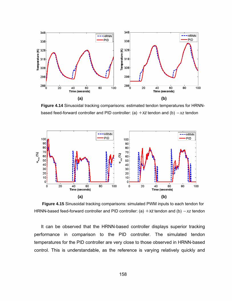
158
(a) (b) Figure 4.14 Sinusoidal tracking comparisons: estimated tendon temperatures for HRNN-
based feed-forward controller and PID controller: (a) xz+ tendon and (b) xz− tendon
(a) (b) Figure 4.15 Sinusoidal tracking comparisons: simulated PWM inputs to each tendon for
HRNN-based feed-forward controller and PID controller: (a) xz+ tendon and (b) xz− tendon
It can be observed that the HRNN-based controller displays superior tracking
performance in comparison to the PID controller. The simulated tendon
temperatures for the PID controller are very close to those observed in HRNN-based
control. This is understandable, as the reference is varying relatively quickly and

159
there is little opportunity to optimize power without sacrificing tracking accuracy.
Hence, it may be concluded that power optimization may not be a factor in tracking
control for rapidly varying references.
4.5 Control of a single-segment robotic catheter
From the discussions in the previous section, it is evident that the HRNN-based
feed-forward controller has potential to optimize power delivery and hence operate
the catheter at lower temperatures. However, the current experimental setup is not
capable of implementing the HRNN-based controller in real-time. Because the PWM
signal generator is embedded within XPC Target system (Figure 4.2), the high
computational requirements of the HRNN-based controller prevent effective PWM
signal generation. However, effective control of the single-segment robotic catheter
can be demonstrated using PI and PID controllers, which have much lower
computation requirements. Even though they may not be power optimal, they are
sufficient to demonstrate other performance measures of the catheter such as
accuracy and control speed.
Both PI and PID controllers were implemented for each of the two decoupled
PCB systems of the single-segment catheter as described in Figure 4.1. Ziegler-
Nichols tuning criteria were employed to optimize the gains of each PI and PID
controller to achieve the best tracking performance. Their performance was
evaluated in terms of regulation control where the tip is commanded to reach a fixed
point in the 3D workspace as well as tracking control where the tip is made to track a
circular trajectory in the 3D workspace.
4.5.1 Regulation control
The closed-loop response (Figure 4.16) of the catheter system to a step
reference of 60refθ = °and 45refφ = ° was measured, along with the control effort

160
(PWM duty cycle) in each plane. It should be noted that at small bending angles (θ
close to the 0), the computation of orientation angle ϕ is extremely sensitive, which
is evident in Figure 4.16b.
(a) (b) Figure 4.16 Experimental step response comparisons: output responses of PI and PID
controllers: (a) Bending angle, (b) Orientation angle
(a) (b) Figure 4.17 Experimental step response comparisons: PWM inputs to each tendon for
PI and PID controller: (a) xz plane and (b) yz plane

161
It can observed from these bending angle responses that both controllers exhibit
quick rise times (~5 seconds) and high accuracy (error< 0.3± ° ) . However, the PID
controller outperforms the PI controller in terms of settling time as the PI controller
exhibits considerable overshoot. However, a comparison of the PWM inputs shows
that the PID controller uses more control effort than PI controller especially in the yz
plane. Both controllers show similar performance in orientation angle response
reaching the given orientation in approximately 5 seconds and achieving high
accuracy (error< 0.2± ° ).
4.5.2 Tracking control
Another control experiment involved having the catheter tip track a circular
trajectory in the 3D workspace. This was accomplished by giving a step input to the
bending angle reference 45refθ = °and ramping the orientation angle reference at a
constant rate of 4.3 deg/second. This reference was intended to simulate a cardiac
ablation procedure using the robotic catheter. During such a procedure, a
cardiologist could map electrical activity in the left atrium of a heart and indicate
discrete points on the atrial surface to define a reference ablation path. Using
computer control, the catheter tip could track a continuous ablation lesion
corresponding to these reference points. Figure 4.18 illustrates the desired ablation
points and actual catheter tip trajectory using a PI controller.

162
Figure 4.18 Three-dimensional representation of the circular trajectory tracking
The responses of each controller in terms of bending angle and orientation angle
are presented in Figure 4.19. The associated control efforts in each plane are
presented in Figure 4.20.

163
(a) (b) Figure 4.19 Experimental tracking of a circular trajectory: output responses of PI and
PID controllers: (a) Bending angle, (b) Orientation angle
(a) (b) Figure 4.20 Experimental tracking of a circular trajectory: PWM magntidues: (a) xz
plane, (b) yz plane
It can be seen from the bending angle response of Figure 4.19a that the PI
controller outperforms PID controller in terms of accuracy. The PID controller seems
to suffer especially near plane transitions ( 0 ,90 , 90 ,180refφ = ° ° − ° ° ). This could be

164
due to the development of slack in the tendons. As slack is taken up, the derivative
of tracking error increases dramatically and induces temporary marginal stability.
The PI controller is free from this problem and hence observed to be more robust.
Based on these results, the ideal controller was chosen as a PI controller.
The tracking and regulation results presented in this section demonstrate the
accuracy and precision with which the catheter can be controlled. Furthermore, real-
time control of the catheter with reference trajectories supplied by a 2 DOF joystick
was also tested. The control performance was found to be excellent both in terms
the speed and accuracy. Although the PI controller is not optimal in terms of power
and thermal characteristics, and does not specifically address nonlinearities such as
occurrence of slack, it is sufficient to verify the feasibility of controlling the proposed
catheter system. Currently, work is underway to implement the HRNN-based
controller on a real time system so that the power optimal control can be performed
while maintaining the speed and accuracy.

165
Chapter 5. Conclusions
This research presents the development of a SMA actuated robotic catheter
including its design, fabrication, modeling and control. It demonstrates the feasibility
of constructing such a device while satisfying performance constraints and
demonstrating excellent control response.
Several candidate designs were evaluated for constructing the single-segment
catheter. Based on the required performance constraints, the most suitable design
was determined to be a central tubular substructure actuated by four SMA tendons.
Superelastic nitinol was the material of choice for the central substructure because
of its large elastic strain range and its ideal flexural and axial stiffness. The catheter
was constructed using a combination of conventional machining and rapid
prototyping.
To analyze and model the dynamics of this catheter, a simpler system was first
considered: a central tube actuated by a single nitinol tendon enclosed by an outer
sleeve. A circular bending model was derived and shown to be accurate even for
large bending angles (± 90°). The heat transfer during actuation of SMA was
analyzed. It was experimentally observed that the actuation is slower for thicker
sleeves and this was explained with a model. Initial efforts to describe SMA
actuation used the Seelecke-Muller-Achenbach model for single-crystal materials.
The parameters for this model were derived from tensile tests of SMA tendons at
various temperatures. The entire system was simulated and the results were
compared to experimental responses, which compared favorably at low frequencies
(0.0043 Hz). However, there were inaccuracies associated with single-crystal
approximation at higher frequencies (0.01Hz).

166
Following this initial modeling effort, it was concluded that improved modeling
techniques were needed to accurately describe the polycrystalline nature of SMA
tendons in real-time. A new modeling approach using recurrent neural networks, so-
called Hysterestic Recurrent Neural Networks (HRNNs), was developed to address
this need. A two-phase version of this HRNN was first demonstrated for modeling
hysteretic systems that possess two distinct phases; this HRNN was experimentally
validated using data collected from a magnetic circuit and a shape memory alloy
actuator. The HRNN was then extended to three phases to fully capture the
constitutive behavior of SMAs. The three-phase HRNN was validated using data
from tensile tests over a wide range of temperatures and stresses.
SMA models described so far require tensile test data of the SMA specimen at
varying temperatures. Conducting such tests for every individual tendon to derive
the model proved to be a tedious task. Consequently, schemes were proposed for
training the HRNN directly on the data from the system under consideration. Such
systems include a SMA-constant mass system, SMA-spring system and also the
Planar Catheter Bending (PCB) System. This approach not only obviated the need
to test every tendon but was also found to be more accurate.
The results of the HRNN illustrate its ability to accurately generalize hysteretic
behavior using relatively few neurons (<250 neurons per tendon). While other neural
network architectures (such as the RBFN) may be trained to approximate the
training data with arbitrary precision, the HRNN demonstrates superior
generalization capabilities to non-training data. Additional benefits lie in the
network’s ability to identify statistical information about the macroscopic material by
analyzing the weights of the individual neurons. Also, the HRNN model has the
ability to run in real-time, making it attractive for use in developing control algorithms.
Shortcomings of the HRNN include the relatively large number of neuron parameters

167
(seven) for general three-phase modeling applications. Relatively sophisticated
training algorithms may be required to expedite training.
Finally, a feed-forward control algorithm based on HRNN was developed to
control the bending of a Planar Catheter Bending (PCB) system. The power and
temperature optimization capabilities of such a controller were demonstrated through
simulations and compared to those of PID controllers. Various hardware limitations
prevented the HRNN-based controller from being implemented in real-time.
Nevertheless, PI and PID controllers were implemented experimentally and were
shown to provide excellent accuracy and bandwidth for the targeted applications.
Changes to the hardware are currently underway to implement the HRNN-based
controller to further enhance tracking capabilities while also optimizing power
utilization so as to keep the catheter temperatures as low as possible.
5.1 Future work
This research provides a foundation for constructing hyper-redundant robotic
catheters with multiple segments and higher DOF that can be operated inside the
body. Future work will focus on achieving this goal by making advancements in the
following areas:
1) Use of electromagnetic location sensors: The dual-camera system used in
this research to provide 3D location of the tip requires line-of-sight to the catheter
which is not ideal for use inside the body. This problem can be circumvented
using 3D electromagnetic sensor systems such as those made by Ascension
Technology Corporation (Burlington, VT) to detect the tip position without
requiring line-of-sight. In fact such sensors are now regularly used in
conventional catheters to collect 3D map of organs inside the body. Future

168
designs of catheters will incorporate these sensors in their design and will be
used for providing position feedback.
2) Custom manufacturing of SMA tendons: The SMA tendons used in this
research are off-the-shelf materials with predefined alloy compositions and
transformation temperatures. In order to reduce the actuation temperatures in the
catheter and keep it within safe limits, the SMA tendons will need to be custom
manufactured to keep the transformation temperatures low.
3) Extension of design to multiple segments: This research describes the
development of a single-segment catheter. This design can be readily extended
to two segments and there are two possible ways to accomplish this. The first
design is involves simply connecting two single-segments serially. The second
approach involves the routing the tendons across segments. In this case though
the tendons extend over both segments, they cause a local bending in only one
of the segments because of the tendons’ optimal distance from neutral axis in
that segment. Construction of catheters with more than two segments requires
development of a addressing bus similar to [23] to deliver controlled power to the
various segments which can be potentially be accomplished using MEMS
techniques.
4) Implementation of model based optimal control algorithms: This research
presents simulated responses of HRNN-based feed-forward controllers. Future
work will involve implementation of the controller on the physical system. Ideas
from optimal control theory could also be incorporated so that designer can make
trade-offs between speed, accuracy and temperature of the system. Also,
alternate methods for real-time implementation of energy-based models for
SMAs were recently presented in [38]. Application of these methods to the
catheter system could also be explored in future.

169
References
1. American Heart Association. Heart disease and stroke statistics: 2007 update at
a glance. http://www.americanheart.org/downloadable/heart/
1166711577754HS_StatsInsideText.pdf
2. H. Eggebrecht, A. Ritzel, C. von Birgelen, A. Schermund, C. Naber, D. B¨ose, D.
Baumgart, T. Bartel, M. Haude, and R. Erbel. Acute and long-term outcome after
coronary artery perforation during percutaneous coronary interventions.
Zeitschrift fr Kardiologie, 93:791–798, 2004.
3. G. R. Barbeau, M. Senechal, and P. Voisine. Delayed abrupt tamponade by
isolated left atrial compression following coronary artery perforation during
coronary angioplasty. Catheterization and Cardiovascular Interventions, 66:562–
565, 2005.
4. Jörg S. Sachweh, Jaime F. Vazquez-Jimenez, Friedrich A. Schöndube, Sabine
H. Daebritz, Hilmar Dörge, Eberhard G. Mühler, Bruno J. Messmer. Twenty
years experience with pediatric pacing: epicardial and transvenous stimulation.
European Journal of Cardiothoracic Surgery, 17: 455-461, 2000.
5. Gertie C.M. Beaufort-Krol, Henk Mulder, Dick Nagelkerke, Tjalling W. Waterbolk,
and Margreet Th. E. Bink-Boelkens. Comparison of longevity, pacing, and
sensing characteristics of steroid-eluting epicardial versus conventional
endocardial pacing leads in children. Journal of Thoracic and Cardiovascular
Surgery, 117:523-528, 1999.
6. A.L.A.J. Dekker, B. Phelps, B. Dijkman, T. van Der Nagel, F.H. van Der Veen,
G.G. Geskes, J.G. Maessen. Epicardial left ventricular lead placement for
cardiac resynchronization therapy: optimal pace site selection with pressure-

170
volume loops. Journal of Thoracic and Cardiovascular Surgery, 127: 1641-1647,
2004.
7. Helmut Mair, Joerg Sachweh, Bart Meuris, Georg Nollert, Michael Schmoeckel,
Albert Schuetz, Bruno Reichart, and Sabine Daebritz. Surgical epicardial left
ventricular lead versus coronary sinus lead placement in biventricular pacing.
European Journal of Cardiothoracic Surgery, 27:235-242, 2005.
8. José L. Navia, Fernando A. Atik, Richard A. Grimm, Mario Garcia, Pablo Ruda
Vega, Ulf Myhre, Randall C. Starling, Bruce L. Wilkoff, David Martin, Penny L.
Houghtaling, Eugene H. Blackstone, and Delos M. Cosgrove. Minimally invasive
left ventricular epicardial lead placement: surgical techniques for heart failure
resynchronization therapy. The Annals of Thoracic Surgery, 79(5): 1536-1544,
2005.
9. Sabine Gabor, Guenther Prenner, Andrae Wasler, Martin Schweiger, Karl Heinz
Tscheliessnigg, Frejya Maria Smolle-Jüttner. A simplified technique for
implantation of left ventricular epicardial leads for biventricular resynchronisation
using video-assisted thoracoscopy (VATS). European Journal of Cardiothoracic
Surgery, 28: 797-800, 2005
10. Prapa Kanagaratnam, Michael Koa-Wing, Daniel T. Wallace, Alex S.
Goldenberg, Nicholas S. Peters and D. Wyn Davies. Experience of robotic
catheter ablation in humans using a novel remotely steerable catheter sheath.
Journal of Interventional Cardiac Electrophysiology, 21 (1): 19-26 January, 2008.
11. Carlo Pappone, Gabriele Vicedomini, Francesco Manguso, Filippo Gugliotta,
Patrizio Mazzone, Simone Gulletta, Nicoleta Sora, Simone Sala, Alessandra
Marzi, Giuseppe Augello, Laura Livolsi, Andreina Santagostino, and Vincenzo

171
Santinelli. Robotic magnetic navigation for atrial fibrillation ablation. Journal of
American College of Cardiology, 47:1390-1400, 2006.
12. H. Oda, M. Oda, Y. Makiyama, T. Kashimura, K. Takahashi, T. Miida, and N.
Higuma. Guidewire induced coronary artery perforation treated with
transcatheter delivery of subcutaneous tissue. Catheterization and
Cardiovascular Interventions, 66:369–374, 2005.
13 . Nabil Simaan. Snake-Like Units Using Flexible Backbones and Actuation
Redundancy for Enhanced Miniaturization. Proc. of the 2005 IEEE International
Conference on Robotics and Automation, 1:3012-3017, 2005.
14. T. Ota, A. Degani, B. Zubiate, A. Wolf, H. Choset, D. Scwartzman and M.A.
Zenati. Epicardial atrial ablation using a novel articulated robotic medical probe
via a percutaneous subxiphoid approach. Innovations, 1(6), 335-340, 2006.
15. Robert J. Webster III, Allison M. Okamura, and Noah J. Cowan. Toward Active
Cannulas: Miniature Snake-Like Surgical Robots. Proc. of the 2006 IEEE/RSJ
International Conference on Intelligent Robots and Systems, 1:2857-2863, 2006.
16. H.D. Hoeg, A.B. Slatkin, J.W. Burdick, Dr. Warren S. Grundfest. Biomechanical
Modeling of the Small Intestine m Required for the Design and Operation of a
Robotic Endoscope. Proc. of the 2000 IEEE International Conference on
Robotics B Automation, 1:1599-1606, 2006.
17. Maria Chiara Carrozza, Paolo Dario and Louis Phee Soo Jay.
Micromechatronics in surgery. Transactions of the Institute of Measurement and
Control, 25: 309-327, 2003

172
18. M. Wieczokek, P. Braun, and W. Schoels. Acquired arteriovenous fistula and
chronic occlusion of the left anterior descending coronary artery in a patient with
previous ablation of a left-sided accessory pathway. Pacing and Clinical
Electrophysiology, 28(8):874–876, August 2005.
19. W. H. Chen, P. Y. Lee, and E.P. Wang. Left anterior descending artery-to-right
ventricle fistula and left ventricular free wall perforation after rotational
atherectomy and stent implantation. Journal of Invasive Cardiology, 17(8):450–
451, August 2005.
20. K. Ikuta, M. Tsukumoto, and S. Hirose. Shape memory alloy servo actuator
system with electric resistance feedback and application for active endoscope.
Proc. IEEE International Conference on Robotics and Automation, 1:427 – 430,
1988.
21. Toshio Fukuda, Shuxiang Guo, Kazuhiro Kosuge, Fumihito Arai, Makoto Negoro
and K. Nakabayashi. Micro Active Catheter System with Multi Degrees of
Freedom. Proc. IEEE International Conference on Robotics and Automation, 3:
2290-2295, 1994.
22. Koji Ikuta, Hironobu Ichikawa, Katsuya Suzuki and Daisuke Yajima. Multi-degree
of Freedom Hydraulic Pressure Driven Safety Active Catheter. Proc. IEEE
International Conference on Robotics and Automation, 1:4161-4166, 2006.
23. K. T. Park and M. Esashi. A multilink active catheter with polyimide-based
integrated CMOS interface circuits. Journal of Microelectromechanical Systems,
8(4):349–357, 1999.

173
24. D. Reynaerts, J. Peirs, and H. V. Brussel. Design of a shape memory actuated
gastrointestinal intervention system. Eurosensors X, pages 1181–1184,
September 1996.
25. H. Takizawa, H. Tosaka, R. Ohta, S. Kaneko, and Y. Ueda. Development of a
microfine active bending catheter equipped with mif tactile sensors. Twelfth
IEEE International Conference on Micro Electro Mechanical Systems, 1999.
MEMS ’99., pages 412 – 417, 1999.
26. Shinji Aramaki, Shinji Kaneko, Kazuhiko Arai, Yuichiro Takahashi, Hideyuki
Adachi and Kazuhisa Yanagisawa. Tube Type Micro Manipulator Using Shape
Memory Alloy (SMA). Sixth International Symposium on Micro Machine and
Human Science, 1:115-120, 1995
27. Y. Haga, T. Mineta, and M. Esashi. Multi-functional active catheter. Sensors
Update, 8(1):147–186.
28. S. Guo, T. Fukuda, F. Arai, K. Oguro, M. Negoro, and T. Nakamura. Micro active
guide tendon catheter system. Proc. IEEE International Conference on Robotics
and Automation, 1:79–84, 1995
29. Shingo Sewa, Kazuo Onishi, Kinji Asaka, Naoko Fujiwara, Keisuke Oguro.
Polymer actuator driven by ion current at low voltage, applied to catheter
system: Proc.The Eleventh Annual International Workshop on Micro Electro
Mechanical Systems, 1998. (1)148-153, 1998.
30. Elie Shammas, Alon Wolf, H. Ben Brown, Jr. Howie Choset. New Joint Design
for Three-dimensional Hyper Redundant Robots. Proceedings of the 2003
IEEE/RSJ Intl. Conference on Intelligent Robots and Systems, 1:3594-3599,
2003

174
31. Ian A. Gravagne, Christopher D. Rahn, ian D. Walker. Large deflection dynamics
and control for planar continuum robots. IEEE/ASME Transactions on
Mechatronics, 8(2), 299-307, 2003
32. Z. Chaudhry and C. A. Rogers. Response of Composite Beams to an Internal
Actuator Force. Journal of Mechanical Design. 114:343-348, 1992
33. G. Wang and M. Shahinpoor. Design, prototyping and computer simulations of a
novel large bending actuator made with a shape memory alloy contractile
tendon. Smart Materials and Structures 6:214-221, 1997
34. D. C. Lagoudas and I. G. Tadjbakhsh. Deformation of active flexible rods with
embedded line actuators. Smart Materials and Structures 2:71-81, 1993
35. U. Icardi. Large bending actuator made with SMA contractile wires: theory,
numerical simulation and experiment. Composites: Part B. 32:259-267, 2001
36. M. Achenbach. A model for an alloy with shape memory. International Journal of
Plasticity. 5:371-395, 1989
37. Olaf Heintze and Stefan Seelecke. A free energy model for the Inner Loop
behavior of Pseudoelastic Shape Memory Alloys. Material Research Society
Proceedings. Vol. 881E cc1.6.1-cc1.6.12
38. Thomas R. Braun. High Speed Model Implementation and Inversion Techniques
for Smart Material Transducers. PhD thesis, North Carolina State University,
Raleigh, NC 2007

175
39. S. Seelecke and I. Muller. Shape memory alloy Actuators in Smart Structures:
Modeling and simulation. Applied Mechanics Review, 57(1):23-46, 2004
40. Qifu Li. Modeling and Finite Element Analysis of Smart Materials. PhD thesis,
North Carolina State University, Raleigh, NC 2006
41. K. Tanaka and S. Nagaki. A thermomechanical description of materials with
internal variables with in the process of phase transformation. Ingenieur-Archiv,
51:287-299, 1982
42. L. C. Brinson. One dimensional constitutive behavior of shape memory alloys:
Thermomechanical derivation with non-constant material functions. Journal of
Intelligent Material Systems and Structures, 4(2):229-242, 1996
43. C. Liang and C. A. Rogers. One-dimensional thermomechanical constitutive
relations for shape memory materials. Journal of Intelligent Material Systems
and Structures, 1:207-235, 1990
44. Shuying Cao, Boweng Wang, Jiaju Zhen, Wenmei Huang, Ling Weng, and Weili
Yan. Hysteresis Compensation for Giant Magnetorestrictive Actuators Using
Dynamic Recurrent Neural Network. IEEE Transactions on Magnetics. 42(4):
1143-1146, 2006.
45. Wei Tech Ang, Fancisco Alija Garmon, Pradeep Kholsa, and Cameron N.
Riviere. Modeling Rate-Dependent Hysteresis in Piezoelectric Actuators.
Proceedings of the 2003 IEEE/RSJ Intl. Conference on Intelligent Robots and
Systems, 2003.

176
46. I.D. Mayergoyz. Mathematical Models of Hysteresis. New York: Spring-Verlag,
1991.
47. Xiaobo Tan, Ram Venkataraman, and P.S. Krishnaprasad. Control of
Hysteresis: Theory and Experimental Results. Technical Research Report. URL:
http://hdl.handle.net/1903/6199
48. H. Hu and R. Ben Mrad. A discrete-time compensation algorithm for hysteresis
in piezoceramic actutators. Mechanical Systems and Signal Processing . 18:
169-185, 2004.
49. A. Cavallo, D. Davino, G. De Maria, C. Natale, S. Pirozzi, and C. Visone.
Hysteresis compensation of smart actuators under variable stress conditions.
Physica B 403: 261-265, 2008.
50. J. Park and I. W. Sandberg. Universal Approximation Using Radial-Basis-
Function Networks. Neural Computation 3: 246-257, 1991.
51. G. Cybenko. Approximation by Superpositions of a Sigmoidal Function. Math.
Control Signals Systems 2: 303-314, 1989.
52. Dimitre Makaveev, Luc Dupre, Marc De Wulf, and Jan Melkebeek. Modeling of
quasistatic magnetic hysteresis with feed-forward neural networks. Journal of
Applied Physics. 89 (11): 6737-6739, 2001.
53. G. Song, V. Chaudry, and C. Batur. Precision tracking control of shape memory
alloy actuators using neural networks and a sliding-mode based robust
controller. Smart Materials and Structures. 12: 223-231. 2003.

177
54. Jeffery L. Elman. Finding Structure in Time. Cognitive Science: 179-211, 1990.
55. A. A. Adly and S.K. Abd-El-Hafiz. Using Neural Networks in the Identification of
Preisach-Type Hysteresis. IEEE Transactions on Magnetics. 34 (3): 629-635,
1998.
56. Sunil Bharitkar and Jerry M. Mendel. The Hysteretic Hopfield Neural Network.
IEEE Transactions on Neural Networks. 11 (4): 879-888, 2000.
57. M. Daniel Tom and Manoel Fernando Tenorio. A Neural Computation Model with
Short-Term Memory. IEEE Transactions on Neural Networks. 6 (2): 387-397,
1995.
58 . Xinlong Zhao and Yonghong Tan. Neural Network based identification of
Preisach-type hysteresis in piezoelectric actuator using hysteretic operator.
Sensors and Actuators A. 126: 306-311, 2006.
59 . Jonas Sjoberg, Qinghua Zhang, Lennart Ljung, Albert Benveniste, Bernard
Delyon, Pierre-Yves Glorennec, Hakan Hjalmarsson, and Anatoli Juditsky.
Nonlinear Black-box Modeling in System Identification: a Unified Overview.
Automatica 31(12): 1691-1724, 1995.
60. Donald W. Marquardt. An Algorithm for Least-Squares Estimation of Nonlinear
Parameters. J. Soc. Indust. Appl. Math. 11 (2): 431-441, 1963.
61. Comparison of EAPs with other actuator technologies. URL:
http://ndeaa.jpl.nasa.gov/nasa-nde/lommas/eap/actuators-comp.pdf

178
62. J. Jayender, R. V. Patel, S. Nikumb, and M. Ostojic. Modeling and Control of
Shape Memory Alloy Actuators. IEEE Transactions on Control Systems
Technology. 16 (2): 279-287, 2008.
63. Xin Yao. Evolving artificial neural networks.Proceedings of the IEEE. 87 (9):
1423-1447, 1999.
64. Da Silva E. P., “Beam shape feedback control by means of a shape memory
actuator”, Materials & Design, 28(5), 1592-1596, 2007
65. N Ma, G Song, and H-J Lee. Precision control of shape memory alloy actuators
with internal electrical resistance feedback using neural networks. Smart Mater.
Struc. 13: 777-783, 2004.
66. Hashem Ashrafiuon, Mojtaba Eshraghi and Mohammad H. Elahinia. Position
Control of a Three-link Shape Memory Alloy Actuated Robot. Journal of
Intelligent Material Systems and Structures, 17, 381-392, 2006
67. V.S. Arpaci, Shu-Hsin Kao, and Ahmet Selamat, Conduction Heat Transfer,
Prentice-Hall Inc., Upper Saddle River, NJ 1999
68. Technical Characteristics of Flexinol Actuator wires. Dynalloy, Costa Meca, CA
69. Theodore R. Kucklick, The Medical Device R & D Handbook, Taylor &. Francis
Group Boca Raton, London, NY 2006
70. URL: http://www.medtronic.com/physician/hf/attain_prevail.html#
71. URL: http://webphysics.davidson.edu/faculty/dmb/PY430/Friction

179
/teflon.html
72. URL: http://www.londonarrhythmiacentre.co.uk/treatments-catheter-ablation-AF-
ablation.html
73. URL: ttp://www.aurorahealthcare.org/yourhealth/healthgate/getcontent.asp?
URLhealthgate="90854.html
74. URL: https://www.clevelandclinic.org/heartcenter/pub/guide/tests/procedures/
pacemaker.htm
75. URL: http://www.kidneyurology.org