Forthcoming in the Journal of Development Economics

Common Factors in Latin America’s Business Cycles Marco Aiolfi Luis A. V. Catão1

Allan Timmermann Goldman Sachs Research Department Rady School, UCSD Asset Management IADB and IMF and CREATES

Final Version: 7 May 2010

Abstract

We develop a common factor approach to reconstruct new business cycle indices for Argentina, Brazil, Chile, and Mexico (“LAC-4”) from a new dataset spanning 135 years. We establish the robustness of our indices through extensive testing and use them to explore business cycle properties in LAC-4 across outward- and inward-looking policy regimes. We find that output persistence in LAC-4 has been consistently high across regimes, whereas volatility has been markedly time-varying but without displaying a clear-cut relationship with openness. We also find a sizeable common regional factor driven by output and interest rates in advanced countries, including during inward-looking regimes. JEL Classification Numbers: E32, F41, N10 Keywords: International Business Cycles, Factor Models, Latin America 1 Corresponding Author. Address: Research Department, Inter-American Development Bank, 1300 New York Ave., Washington DC 20577. Phone: (202)6233587. E-mail: lcatao@iadb.org. We thank Ayhan Kose, Simon Johnson, Gian Maria Milesi-Ferretti, Adrian Pagan, Valerie Ramey, Luca Sala, Jeffrey Williamson, as well as two anonymous referees for extensive comments and suggestions on earlier drafts. We are also grateful to Nathan Balke and Christina Romer for generously sharing their data with us, and to seminar participants at the Fundação Getulio Vargas in Rio de Janeiro, IDB, IMF, PUC-RJ, UC San Diego, University of Manchester, the World Bank, and at the 2005 EHES and LACEA meetings. Timmermann acknowledges support from CREATES, funded by the Danish National Research Foundation. The views expressed in this paper are those of the authors alone and do not necessarily reflect the views of the institutions to which the authors are affiliated.

- 1 -

I. INTRODUCTION

Business cycle volatility can arise from a variety of sources and may be exacerbated by distinct economic policy regimes, possibly reflecting slowly-evolving institutional factors (Acemoglu et al. (2003)) and different degrees of financial and trade openness (Kose, Prasad, and Terrones (2006)). This suggests that important insights can be gained from long-run data spanning a variety of policy regimes and institutional settings. Yet there is a striking dearth of systematic work along these lines for most countries outside North America and Western Europe.

A key constraint to this line of research has been lacking or patently unreliable GDP data for developing countries. While the work of Maddison (2003) has made important strides in filling some gaps and making long-run data more easily accessible to the profession, important deficiencies remain. For most developing countries, Maddison's pre-World War II data is either provided only for select benchmark years or compiled directly from secondary sources relying on annual data from a very limited set of macroeconomic variables and often using disparate methodologies to construct GDP estimates.

Partly due to such data constraints, one region that has been particularly under-researched from a historical business cycle perspective is Latin America. This gap is striking not only because the region is highly volatile and the question of what drives such volatility is of interest in its own right; it is also striking because the region comprises a large set of sovereign nations which historically have gone through dramatic changes in policy regimes and institutions relative to other developing countries in Africa and Asia (many of which only became independent nations in recent decades), thus providing a rich context for assessing business cycle theories. Indeed, Latin America is notoriously absent in the historical business cycle studies by Sheffrin (1988), Backus and Kehoe (1992), and A’Hearn and Woiteck (2001), and only Argentina is covered in more recent work (Basu and Taylor (1999)). Instead, existing work on business cycles covering Latin America has spanned much shorter time periods and/or focused on specific transmission mechanisms (Engle and Issler (1993); Mendoza (1995); Kydland and Zarazaga (1997); Agénor, McDermott and Prasad, (2000)). A corollary of this gap in the literature is the absence of any formal attempt to establish a reference cycle dating for these countries similar to that available elsewhere as well as to relate such a reference cycle to the world business cycle.

This paper seeks to fill some of this lacuna. Our contribution is threefold. First, we construct a new business cycle index for each of the four largest Latin American economies – Argentina, Brazil, Chile, and Mexico (“LAC-4”) – spanning 135 years and covering roughly 70 percent of Latin America’s GDP. Our data cover an extensive set of aggregate and sector variables compiled from a wide range of historical sources – both primary and secondary; as some of these series have been constructed from scratch, this has resulted in an unprecedentedly long and comprehensive database for each of the four countries. Moreover, our estimates are built on an econometric methodology that efficiently aggregates the business cycle content of the individual series, combining common factor extraction with “backcasting” procedures to build new country indices of aggregate economic activity. These new indices provide a measure that is germane to the business cycle concept employed in the work of Burns and Mitchell (1946) which underlies the widely used NBER reference cycle

- 2 -

indicator for the United States. To the best of our knowledge, this is the first time such a methodology is used in reconstructing historical business cycle indices for a single country as well as for a region.

The second and more central contribution of the paper lies in using the new data to formally characterize various stylized business cycle facts for each of these economies. We address three questions. First, how volatile has LAC-4 been relative to other countries during periods of greater trade and financial integration with the world economy (such as during the pre-1930 gold standard and the post-1970s period) as well as during the inward-looking regimes of the 1930s through the early 1970s? Second, how persistent have macroeconomic fluctuations been in those four countries? Since country risk and the gains from stabilization policy both rise when the underlying volatility and persistence of output shocks increase, it is important to have good measures of both. Third, since our business cycle index is built from various macro, financial and sector output indicators, our data also allows us to establish where such volatility and persistence come from. In doing so, we examine whether “stylized facts” for other economies regarding the pro- or counter-cyclicality of key variables such as the trade balance, fiscal policy, inflation and real wages also hold for LAC-4.

The third set of results focuses on the issues of international business cycle transmission and common cross-country factors. Using the classic Bry-Boschan algorithm for business dating and the Harding-Pagan (2002) concordance index, we measure the extent of business cycle synchronicity between the four countries. Then, we identify the common regional cycle through a dynamic common factor extraction from the pool of the individual country series – a novel approach that more fully utilizes information from existing country data. Having identified the common regional factor, we then examine how it is related to global factors such as fluctuations in world output, interest rates and commodity terms of trade. Finally, we use SURE regressions to orthogonalize the individual country cycles to these global factors so as to gauge the extent of country-specific shocks in accounting for national cycles.

The main findings are as follows. Our new index of economic activity is shown to very closely track existing real GDP data from the full set of national account estimates beginning after World War II (WWII henceforth). Our “backcasting” procedure also appears to be robust to structural change and the new indices closely track qualitative historical narratives of cyclical turning points in the four countries. This suggests that our business cycle indices provide reasonably accurate measures of pre-WWII cycles in Argentina, Brazil, Chile, and Mexico.

The new indices allow us to uncover the following stylized facts. The average business cycle volatility in all four countries has typically been much higher than in advanced economies and higher than in many emerging markets. Moreover, there were substantive differences across policy regimes. Latin American volatility was high during the openness regimes of the pre-1930 era, i.e., precisely during the formative years of key national institutions. With the exception of Chile, cyclical volatility then dropped during the four decades following the Great Depression, before bouncing back again in the 1970s and 1980s—when these economies again became more open to international capital markets—but then declined sharply, amidst continuing financial and trade openness. Throughout the past century and a half, output persistence has been consistently high, with large shocks giving rise to a striking

- 3 -

combination of high amplitude and long duration of output fluctuations relative to advanced country standards. Overall, this indicates no clear-cut unconditional relationship between openness on the one hand, and cyclical volatility and persistence on the other.

Some business cycle regularities are similar to those observed elsewhere while others differ. External terms of trade have been strongly procyclical, the trade balance counter-cyclical, and fixed investment has been several times more volatile than output. We also find that fiscal policy has been broadly procyclical and highly volatile in LAC-4—despite some dampening during the 1930-70 inward-looking regimes. In contrast, we find that inflation historically has been counter-cyclical and real wages broadly procyclical. Aggregate persistence is mainly accounted for by shocks to fixed investment, government spending, and broad money, with manufacturing and service output resulting to be far more persistent than agricultural output.

Finally, business cycles in the LAC-4 economies have been reasonably correlated throughout, including during the inward-looking policy regimes when trade and capital controls were very stringent. Global factors associated with commodity terms of trade, interest rates and output fluctuations in advanced countries account for much of such commonality, with the respective shares varying by country and period.

The remainder of the paper proceeds as follows. Section II sketches the econometric framework and Section III reports estimates and robustness checks on our methodology. Section IV presents the business cycle dating chronology for all four countries and stylized facts regarding persistence and volatility across policy regimes. Section V discusses cross-country synchronicity based on the common regional factor extraction, and the role of global and intra-regional factors therein. Section VI concludes.

II. METHODOLOGY

A key ingredient of this paper is the construction of a consistent set of time series that permits more accurate inter-period and cross-country comparisons of business cycle dynamics in LAC-4. The absence of a full set of national income accounts for the pre-WWII period poses a major challenge. While previous researchers have tried to fill this gap by building “unofficial” GDP indicators for this early period, these suffer from the insufficient output coverage of the underlying series, as well as the use of disparate reconstruction methodologies. In the extended working paper version, we discuss in detail how these earlier reconstruction attempts produced series of uneven quality that often do not match the historical narrative of cyclical behavior in these economies (Aiolfi, Catão and Timmermann (2006)). Another difficulty is that the dramatic shift in both the output coverage and the construction methodology between pre- and post-WWII series could greatly undermine the accuracy of any inter-period comparisons between the two eras. This has been argued to be the case even for a country with a wealth of historical data such as the US (Romer (1989)).

The reconstruction procedure laid out here addresses both of these limitations. For each country we put together a broad set of indicators that are well-known to co-move closely with aggregate output and for which we have information spanning the pre- and post-WWII

- 4 -

periods. This potentially ensures greater consistency of inter-period comparisons since they are based on the same set of indicators per country. Our selection of variables (basically dictated by data availability) also facilitates inter-country comparisons within LAC-4 since it is quite similar across countries. These variables include capital formation, government revenue and expenditures, sector output series, as well as external trade and a host of financial variables. Since Latin American economies have historically been highly dependent on global capital markets and demand from outside trading partners, interest rates and cyclical output in advanced countries are also included. Our final data spans 20-25 variables per country between 1870 (1878 for Mexico) and 2004, with some variables being built from scratch based on research with primary data sources. Sources and specifics of the data construction are provided in Aiolfi, Catao and Timmermann (2006). To the extent that these variables correlate closely with aggregate economic activity, efficient aggregation of this information should yield a reasonably accurate measure of the national business cycles.

To efficiently aggregate the information content of this dataset, we use an information extraction methodology that builds on the idea – dating back at least to Burns and Mitchell’s (1946) seminal work – that any sufficiently broad cross-section of economic variables shares at least one common factor. This approach has two key advantages. First, it allows for the existence of strong linkages between economic activity across main sectors due to common productivity, preference and policy shocks, including across countries. Once we have a sufficiently wide and long panel of economic variables that are at least in part driven by these (typically unobservable) shocks, the common factor approach extracts information about macro shocks with minimal resort to an a priori theoretical structure.

The second advantage pertains to aggregation efficiency. The presence of errors in the measurement of activity levels in many sectors can make simple aggregation highly inaccurate. This is more likely to be the case with developing country data and with series going far back in time. In contrast, provided that such measurement errors are largely idiosyncratic, they are filtered out in the factor construction (Stock and Watson, (2002)). Thus, one should expect a common factor methodology to be particularly useful for the construction of a business cycle index when some of the constituent series adding up to a target variable (such as GDP) are lacking, or when those series are suspected to be seriously mis-measured. Both are true for LAC-4 pre-World War II data – with measurement problems also likely to plague at least some of the post-WWII data as well.

The final component of our reconstruction methodology consists of scaling these factors to a measure of aggregate economic activity over the period when this measure becomes available. This is done by regressing the extracted common factors on real GDP over the post-1950 period. The respective estimated coefficients are then used to “backcast” real GDP for the pre-1950 period, with the expected value of the respective country regressions being used as an indicator of the aggregate cycle for the post-1950 period as well. This ensures greater consistency of inter-period comparisons of business cycle dynamics.

We provide next a brief description of the mechanics of our approach.

- 5 -

A. Dynamic Factor Extraction

Let tX be a vector of de-meaned and standardized time-series observations on N economic variables observed over the sample 1,...,t T= . Assuming that tX admits a common factor representation, we can write:

Xt = ΛFt + et (1)

where Ft =(ft,….,ft-s) contains the current and lagged dynamic factors, ft, and et comprises the idiosyncratic disturbances. In practice the factors are typically unobserved and extraction of them from the observables ( )tX requires making identifying econometric assumptions. As is typical in the literature, we assume that the errors te are orthogonal with respect to the current factors, tf , although they can be correlated across series and through time. In addition the factors are only identified up to an arbitrary rotation.

In our application N is quite large so we adopt the non-parametric method based on static principal components (Stock and Watson (1999)). A principal component estimator of the factors emerges as the solution to the following least squares problem:

( ) ( )'1

, 1min

T

t t t tF tT −

Λ=

− −∑ XΛF X ΛF

subject to the restriction = Ι'Λ Λ . The solution to this problem { }ˆ ˆ, tΛ F takes the form

'

,

ˆ

ˆt t

v

v

=

=

Λ

F X (2)

where v comprises the eigenvectors corresponding to the largest eigenvalues of the variance-covariance matrix for the X variables. The resulting estimator of the factors, ˆ

tF , contains the static principal components of tX .

This estimator requires that all variables entering the dynamic common factor specification are stationary. We are interested in the cyclical component of aggregate activity, so we employ two alternative approaches to ensure this. With the exception of the inflation rate, real interest rates, and the ratios of export to import value which are already stationary, we de-trend the remaining series by the standard Hodrick-Prescott filter, with a smoothing factor set to 100, as is common practice with annual data (e.g. Backus and Kehoe (1992); Kose and Reizman (2001)). The second approach to detrending considered here is the symmetric moving average band-pass filter advanced by Baxter and King (1999). Following common practice with annual data, we set the size of the symmetric moving average parameter to three but use a large bandwidth ranging from 2 to 20 years so as to avoid filtering out the longer (12–20 year) pre-war cycles first documented by Kuznets (1958) for the United States. As shown below, both detrending methods yield very similar results. Since we take natural

- 6 -

logs of the respective series, the resulting de-trended component or “cycle” measures percentage deviation of the actual series from trend. Letting y stand for aggregate output, this is equivalent to defining the cycle as log( ) log( ) ( / 1)actual trend actual trendy y y y− ≈ − , which is the so-called “output gap”, i.e., the percentage deviation of actual output from its trend.

B. Backcasting Regressions

The common factors are of interest in their own right since they provide broad-based measures of economic activity. However, often particular interest lies in relating them to a specific economic variable such as real GDP. As discussed above, reliable data on this variable may only be available over the later part of the sample and, even then, the series may be subject to considerable measurement error and/or discontinuities in data collection and aggregation procedures in national income account construction.

To deal with this we use backcasting to create a new historical time-series of cyclical aggregate output. In particular, we estimate the following backcasting equation using contemporaneous factor values:

' ˆt t ty α ε= + +βF (3)

Coefficient estimates are based on the post-1950 sample for which data of sufficient quality are available on ty . Provided the parameters in (3) remain constant, we can then backcast cyclical output over the earlier sample for which estimates of the factors are available but data on aggregate output is missing.

III. THE NEW BUSINESS CYCLE INDICES

A. Estimates and Comparison with Previous Indices

Table 1 shows the estimated factor loadings for the first two factors extracted using the Stock and Watson (SW) procedure in equation (2). We report only the first two factors since the addition of further factors contributes only marginally to the total variance of the panel with the exception of one country (Brazil) for which the third factor turns out to be important. As discussed above, in all cases the factors are extracted from a panel where the series have been detrended by the HP-filter with exception of series that are known to be stationary (inflation rate, real interest rates, and the export to import ratio). To check for robustness we computed the same SW factors when the non-stationary underlying series were detrended using the Baxter-King (BK) band-pass filter. Figure 1 shows that these de-trending approaches yield very similar results. Given that the HP-detrending has been more extensively used in related studies (Backus and Kehoe (1992); Kydland and Zarazaga (1997); Kose and Reizman (2001); Neumeyer and Perri (2005)) and in light of some of its advantages relative to other methods that under-weigh low frequency components of the data (which are important during episodes of persistent growth accelerations/decelerations of the type described in

- 7 -

Hausmann, Pritchett, and Rodrick (2004)), we stick to HP-detrending through the remainder of the paper.

Factors extracted from a panel on a variety of variables are typically not straightforward to interpret and are only identified up to an arbitrary rotation. Yet, the estimated factor loadings do offer important clues in this respect. The first factor (labeled F1) can be interpreted as a broad measure of cyclical activity since it loads positively on indicators that are well-known to be procylical, such as sectoral output, fixed capital formation, import quantum and real money, all measured in deviations from their respective long-term trends. Corroborating this interpretation, the first factor also bears a strong positive correlation with the GDP cycle during periods where official GDP data is available.

The interpretation of the second factor (F2) is less clear-cut. For Argentina, Brazil and Chile, this factor assigns large loadings to money, the domestic interest rate and the real exchange rate (also entered in deviations from trend). Thus, it can be broadly interpreted as an index of monetary conditions. In the case of Mexico, the largest loadings are observed on the variables capturing external linkages such as the terms of trade, the real exchange rate or import volume. This is suggestive of non-trivial differences between the economies regarding business cycle transmission—a point to which we return in Section V.

Ultimately our interest lies in reconstructing a measure of cyclical activity. To this end, Table 2 reports the 2 'R s of regressions of de-trended actual GDP on the factors across different factor model specifications. The results cover the period 1950–2004, when full national account estimates are available for all four countries. As with the bulk of the series entering the alternative factor specifications, actual GDP is also expressed in deviations from an HP trend. Correlations in Table 2 thus gauge the extent to which the various factor models span the real GDP cycle or “output gap”. To indicate the sensitivity of the results to the adopted econometric methodologies, we present results both for the all-regressor approach—which maximizes the 2R by projecting cyclical GDP on all variables—and for the Stock and Watson approach using between one and four common factors. As we shall see below, the high in-sample fit of the all-regressor, “kitchen sink” approach comes at the cost of overfitting the data and seemingly producing poor out-of-sample performance. Overall, linear projections of the GDP cycle on the various factors yield a tight fit for Argentina, Chile and Mexico, with 74–88 percent of the variance of the real GDP cycle explained by the first two factors alone. The fit for Brazil is relatively worse, but including the series on agricultural and manufacturing output (only available from 1900 onwards) raises it above 80 percent.

For each country, the left graphs in Figure 2 show our new indices and previously existing estimates of cyclical GDP over the period 1870–1950, while the right graphs compare our indices with the (HP-filter) de-trended real GDP taken from the most recently revised set of national accounts for 1950-2004. The close proximity between our new common factor-based indices and the detrended GDP derived from national accounts for the post-1950 period is clear from these plots –visual differences only emerge during rare and extremely large spikes such as in Brazil in 1961–62 and 1980. Thus, it is plain that our indices generally very closely track actual cyclical GDP whenever better quality estimates of the latter are available from official national accounts.

- 8 -

Figure 2 further shows that the factor-based estimates often differ substantially from estimates generated by the all-regressor (or “kitchen sink”) least squares regressions. Since the latter is the furthest away from the observations produced by better quality out-of-sample estimates (as for Argentina over 1935–49, Chile during 1940–49, and Mexico 1925–49), this strongly cautions against the use of a kitchen sink approach by researchers in the reconstruction of earlier GDP data. Moreover, the new indices differ substantially from previous authors’ estimates of pre-war GDP, including Maddison’s (2003). While such discrepancies are strikingly large for pre-1930 Brazil and Mexico during 1907-29, they are not negligible either for Argentina and Chile. Since our pre-WWII estimates are very robust to a variety of econometric tests as shown next, and also closely track descriptions of economic turning points from these countries’ historiography – something that previous indices do not (see section V) – this suggests such discrepancies between our indices and previous historical estimates are in all likelihood due to deficiencies in the latter.

B. Robustness to Structural Change

Just as out-of-sample forecasts rely on an implicit assumption that certain relationships between predictor variables and the target variable remain constant over the forecasting period, backcast estimates of economic activity measures also require this assumption. Yet, widespread perception that Latin American economies have witnessed dramatic structural changes due to, e.g., economic liberalization cycles, high inflation bouts, and extensive time inconsistency in policy-making makes it particularly important to investigate whether the accuracy of our new business cycle index is compromised by the potential instability of the factor loadings and of the regression coefficients in (3).2

This has implications for the stability of the regression coefficients in (3). Suppose that the relationship between inflation and GDP changes over time as countries move through distinct monetary and exchange rate regimes. As discussed further later on, there are theoretical reasons why inflation is mostly counter-cyclical in these countries but can also be pro-

Stock and Watson (2002) provide both theoretical arguments and empirical evidence that principal component factor estimates are consistent even in the presence of temporal instability in the individual time-series used to construct the factors provided that this instability averages out in the construction of the common factors. This occurs if the instability is sufficiently idiosyncratic to the various series and the underlying panel is broad enough that the instability in the relationship between the factor and one or more of the underlying series (20 to 25 per country in our panel) is compensated elsewhere in the panel.

2 Latin American economies are often perceived to have been subject to far-reaching structural changes with major bearings on average growth as well as the cross-country heterogeneity thereof. However, Chumacero and Fuentes (2006) find that, after controlling for external shocks and a measure of distortions, the behavior of per capita GDP in much of the region has been reasonably stable. This is broadly consistent with the results presented in Section IV which show that common external factors have accounted for much of the cyclical variation in aggregate output in LAC-4 over the period 1870-2004.

- 9 -

cyclical at times. The net effect is a weakening of the relationship (and hence the magnitude of the loading) between inflation and the factor(s) which are pro-cyclical. As discussed above, since the first factor (F1) is strongly procyclical in our estimates, this implies that the loading of inflation on this factor will be weakened. This is precisely what the estimates in Table 1 suggest. To the extent that there is more than one factor (in our case we have two or three factors by country), the change may be absorbed by a stronger inflation coefficient in the remaining factors. Since the regression in (3) includes more than one factor (two for Argentina, Chile and Mexico and three for Brazil), this shift in the underlying relationship should be captured by the inclusion of extra factors. An analogous reasoning applies to changes in lead-lag relationships between the underlying variables: as emphasized by Stock and Watson (2002), the inclusion of extra factors can mitigate such structural change problems. In the limit, if a specific series bears too erratic a relationship to the target variable (real GDP in this case), then the respective series will have a small loading on the various extracted factors and hence the effects of such instability on the coefficients in the back-casting equation (3) will be quantitatively unimportant.

We buttress this conceptual discussion with an empirical evaluation of the robustness of our parameter stability assumption using four batteries of tests. First, we inspected the minimum and maximum value across different specifications of the back-casting equation, (3), that vary the number of static factors between two and three; used different samples for factor estimation, where a new sample is adopted if new time series become available (Argentina: 1870–2004, 1875–2004, 1900–2004; Brazil: 1870–2004, 1900–2004; Chile: 1870–2004; Mexico: 1878–2004); and adopted two different panels of data, one including external variables while the other excludes these. For each country this yields between 4 and 24 different specifications. However, with the exceptions of Brazil in 1890–91, 1986 and 1989, Chile in 1929–32 and Mexico in 1916, the range of estimates is very narrow; and even for those outlier observations, all estimates point in the same direction. As it turns out, all indications are that little has changed over time. This congruence is unlikely to hold if the factor loadings were subject to structural breaks.

Second, we also check for the stability of coefficients in the regression of the factors on the cyclical component of real GDP. This was done by re-estimating (3) for the period 1961–2004 (instead of 1950–2004) and recursively rolling back the estimation to the last point for which reasonably reliable data on real GDP exists.3

3 Pre-war data on GDP for all the countries are considerably less reliable than official post-war data, but we thought it worthwhile to compare the stability of the back-casting regression coefficients against some of the existing pre-war data as a further robustness check. Given that data for Argentina, Brazil and Mexico from 1920 onwards appear to be of much better quality (albeit still relying on partial production data) than pre-1920 data, we extended the recursive stability test to 1920 using this data.

Figure 3 shows that the back-casting coefficients are reasonably stable over the 1930–60 period (1940–60 for Chile). Only in the case of Mexico between 1921 and 1925 is there evidence of some instability. This should not be surprising since the real GDP figures used to compute the recursion over the early post-

- 10 -

revolutionary period for Mexico are likely to be marred by measurement problems before the Banco de Mexico centralized the compilation of macroeconomic data in 1925.

Third, we check the sensitivity of our results to an arguably stricter test: we estimate the factor loadings over two different sub-samples – 1870-1950 and 1950-2004 (the latter being marked by various bouts of high- and hyper-inflation, as well as heavy government intervention). We then check how the first two factors of each estimation correlate with the corresponding pair over the other sub-sample, and re-estimate the back-casting equation swapping them. The correlations for the first factor (using the original versus the swapped loading coefficients) show that this makes little difference for three of the four countries. The differences are only sizeable for the second factor in Argentina and Chile. Since the coefficients on the projections of the second factor on GDP are generally very low, these differences only affect the fitted values in the back-casting equation (3) in a minor way.

Fourth and finally, in a Bai-Perron (1998) regression of growth rates of real GDP on our factors extracted from the HP-filtered series, we find little evidence of structural instability. In fact, there is only evidence of breaks for Chilean GDP growth for two years with extreme outliers in the pre-1950 sample, where the underlying level series (which we used to compute growth rates) are less reliable.4

IV. POLICY REGIMES AND BUSINESS CYCLE FACTS

Overall, the results above make an important point. Even when the common factors are extracted for countries where changes in economic structure are deemed to have been substantial, they track the real GDP cycle well. This may not be surprising since we selected variables that economic theory suggests are closely related to cyclical activity and a panel which is broad enough so that instability in the linear relationship between individual indicators and the aggregate cycle may be offset elsewhere in the panel.

A. Dating LAC-4 Cycles

Armed with business cycle indicators for the four countries, we now turn to the stylized facts, starting with the dating of turning points and thus establishing the typical cyclical lengths. A classic device to this end is the Bry and Boscham (1971) algorithm. It consists of a sequence of procedures starting with the search for extreme values in order to eliminate (near-) permanent jumps in the series associated with outliers, followed by the use of centered moving averages and the search for local maxima or minima within a particular window. Table 3 shows the peaks and troughs of the business cycles for the individual countries. To permit the identification of both shorter and longer cycles, Panels A and B of Table 4 report results based on two-year and six-year windows, respectively. As expected, the algorithm identifies peaks and troughs that are broadly consistent with a visual inspection of individual country plots (see Figure 2 as well as Figure 5 below). When the narrow window is used, the average duration of the cycle is shorter overall, and the more so during the post-WWII era.

4 These test results are not reported here but are available from the authors upon request.

- 11 -

Using a longer window, Panel B indicates that the pre-WWII cycle is dominated by the long swings of the type first analyzed by Kuznets and subsequently by Solomou (1987). This evidence of lengthy cycles is corroborated by spectral density function estimates below.

B. Persistence Patterns

Further evidence that LAC-4 output fluctuations have been relatively protracted is provided by spectral analysis. Panel A in Table 4 reports peak values of the spectral density function of our business cycle index (standardized by scaling the respective series by their variance times π) as well as the point in the frequency spectrum (the inverse of which thus being the cyclical length T) where they occur. LAC-4 cycles were quite lengthy throughout 1870-2004. The average duration was even longer in the pre-WWII period, when the dominant cyclical length was 14 to 16 years.

The estimated spectral density function allows us to further address how the frequency ranges contribute to the total variability of our index, i.e., the extent to which shorter vs. longer fluctuations account for the total variability of de-trended output. Panel B in Table 4 shows that much of the aggregate output persistence in LAC-4 is accounted for by the lower range of the frequency spectrum: over the 1870-2004 period, shocks associated with the shorter cycles (3-6 years) accounted for between 12% and 20% of the total variability in de-trended output, whereas those related to longer cycles (7 to 12 years) accounted for between 43% and 53%. Consistent with the evidence on the shortened business cycle after WWII, the contribution of short-run fluctuations doubled post-1946. Yet, with the exception of one country (Argentina), the low frequency range of the spectrum continues to account for a higher share of the variability of de-trended output.

One benefit of having an index of aggregate activity built from a broad array of macro and sector output indicators is that it enables us to trace the sources of aggregate persistence in these economies. Table 5 reports standard ARIMA(p,I,q) measures of shock persistence

(“P”) for the series in our country panels, with 1

1

1 ...1 ...

q

p

Pθ θρ ρ

+ + +=

− − −, where qθ is the coefficient

on the moving average (MA) component of order q and pρ is the coefficient on the auto-regressive (AR) term of order p. I=0 for stationary series such as spreads, inflation, and real interest rates, and I=1 otherwise. Because maximum likelihood ARIMA estimates are sensitive to outlier specifications and standard model selection criteria yield disparate results, for each variable and country, four ARIMA specifications were estimated [(1,1,1), (2,1,2), (2,1,0), and (0,1,2)]. For each country and each variable the entries in the table refer to the median estimate across these model specifications. Combining these univariate estimates with the loading on the coefficients of each variable on the factors in Table 1, one can approximately gauge where much of the aggregate persistence comes from. Further, because these ARIMA-based persistence measures are not based on de-trended data, they provide an even broader measure of aggregate persistence than the spectral estimates above and the AR(1) measures presented below.

During 1870-2004, the sector breakdown in Table 5 indicates that manufacturing output and services (transportation and communication) typically have above-average persistence (often

- 12 -

higher than one). As these sectors generally load heavily on the economy-wide pro-cyclical factor and on GDP, they account for the high aggregate persistence in these countries. Agricultural output is typically the least persistent of all series. Much of the aggregate persistence is driven by fixed capital formation, government spending, terms of trade and real M2. Real wages and imports are also quite persistent. Some of the domestic output persistence is clearly imported, as foreign real GDP also has persistence above some domestic variables.

Limiting the sample to the post-WWII period reduces the precision of the maximum likelihood estimates of the MA components. Yet, the relative ranking remains largely robust. Notable differences pertain to the behavior of sovereign spreads, suggesting that country risk in the post-WWII period has become more persistent, and a decline in terms of trade persistence. Another advantage of looking at this sample is the availability of official GDP figures which enable us to report univariate measures for the overall persistence of GDP – something that we evaded for the pre-WWII period due to the low quality of estimates of trend GDP. Overall, real GDP persistence is on average above one and, in two of the four countries (Brazil and Mexico), it exceeds two.5

We refine these results by focusing on cyclical persistence across policy regimes and providing a broad international comparison in this context. We categorize the sample into three regimes. The first, which spans the early globalization in the 1870s era through the onset of the 1930s Great depression, was characterized by tight financial and trade integration with the world economy. There were no foreign exchange or capital controls, quantitative trade restrictions were virtually absent, with export and import shares in GDP at historical highs, and government size substantially lower than at any time since. This outward-looking regime was sharply reversed in the subsequent four decades through the early 1970s, starting with stringent capital controls in 1930-31 and followed by a complex system of trade restrictions. In the wake of the breakdown of the Bretton-Woods system in 1971 and the re-opening of world capital markets to developing country sovereign borrowing from the mid-1970s, financial openness in LAC-4 rose again. After some temporary set-back during the 1980s debt crisis, trade openness greatly intensified from the late 1980s. In light of these developments, we split the sample into pre- and post-1930 as well as pre- and post-1970 periods, including a further split from 1987. The latter is also instrumental in allowing us to address the recent debate on the existence of a “Great Moderation” in global business cycle volatility since the mid-1980s.

Similar measures for the US over the same period yield P=1.01, whereas for the weighted real GDP of the largest advanced economies P=1.28. So, the various measures based on our business cycle index indicate that output persistence is high in LAC-4 and this conclusion is not overridden by overall (non-detrended) measures. In other words, the inference that output is highly persistent in LAC-4 does not depend on one’s view of what is cycle and what is trend. This is in line with the findings of a recent and growing empirical literature on macroeconomic fluctuations (Aguiar and Gopinath (2007); Cerra and Saxena (2008)).

5 The fact that univariate measures of GDP persistence can yield higher figures than its component parts is well-known and explained by aggregation biases (Pesaran et al. (1993)).

- 13 -

Tables 6 and 7 report a classical measure of cyclical persistence – the slope coefficient of a regression of the business cycle index on its one-year lag (the so-called AR1 measure). Corroborating the earlier findings on the high output persistence in LAC-4, the respective AR(1) estimates of cyclical persistence are reasonably high throughout 1870-2004. Persistence was particularly high in LAC-4 in the pre-1930 era as well as during the 1970s and 1980s. Furthermore, if we discount major country-specific outliers (such as Argentina around the mid-1970s and Mexico’s unusually swift recovery from the 1994-95 crisis) and focus on the common regional factor (extracted as discussed in Section V), cyclical persistence has been even higher: the respective LAC-4 AR(1) coefficient is 0.74 for 1879-2004 as a whole, dropping to 0.60 over 1930-70 and then rising to 0.71 during 1971-2004. These regional averages are well above the benchmark values for several advanced countries and other emerging markets.

C. Volatility

In addition to AR(1) measures, Tables 6 and 7 also report standard deviations of the cycle across periods and countries. These corroborate the perception that Latin America has been a more volatile region than countries deemed advanced by today's definition, as well as relative to Australia, Canada and Japan that were considered “emerging economies” in the pre-war world. However, this volatility gap between the two groups has changed significantly over time and across policy regimes. The four Latin American countries were clearly far more volatile than both advanced and new world (“NW”) countries in the pre-1930 period. Starting from the Great depression, however, this gap was reversed (See Table 7, panel A). In the wake of the 1929–32 world slump, World War II, and subsequent geopolitical dislocations, global volatility rose to historical highs. As noted above, it was precisely during this period that capital and trade controls were enacted leading to significant drops in trade shares and net capital inflows to GDP. So, our estimates indicate that such inward growth policies did succeed in fending these countries off from global instability. Interestingly, LAC-4 volatility declined not only relative to advanced countries but also relative to other developing countries such as India, Indonesia, Korea, Malaysia, Sri Lanka, South Africa, Taiwan Province of China, and Turkey. Interestingly, this lower volatility did not come at the expense of lower growth during that period, though a case has been made that price distortions due to inward-looking regimes impaired growth later on (Taylor (1998)).6

As output gap volatility came down in the advanced countries from the 1960s, cyclical volatility in Latin America rose again; only in the post-debt crisis period has LAC-4 cyclical volatility declined markedly compared to earlier levels. Despite being low relative to its historical record, business cycle volatility in Latin America has remained higher than in advanced countries as well as relative to Asian developing countries during 1988-2004. Rolling standard deviations of the output gap in Figure 4 summarize this broad overview of

6 The LAC-4 median of the ratio of growth volatility by mean growth (coefficient of variation) dropped to 1.0 during 1930-1970 (despite the Great Depression and WWII) from 1.66 before 1930, and up to 1.14 in 1971-2004. More recently, however, it dropped to 0.9 in 1988-2004. Similar inferences obtain using the un-weighted regional mean rather the median.

- 14 -

volatility trends in the region by plotting both individual country trends as well as that of the common regional cycle (extracted as discussed in Section V). Buttressing these descriptive statistics, more formal ARCH tests for each of the four countries generally reject the hypothesis of no time-series clustering of output volatility.

A key question from the viewpoint of business cycle transmission is what drives aggregate volatility. As with the previous analysis of persistence, the broad range of macro variables contained in our long dataset helps shed light on the volatility sources. As before, we break the sample down by policy regimes. Table 8 highlights some stylized facts that have been stressed in previous studies (Backus and Kehoe (1992); Mendoza (1995); Basu and Taylor (1999); Agénor, McDermott and Prasad (2000)). First, cyclical volatility in fixed investment is much higher than that of output. Second, government spending volatility is higher than output volatility. For all four countries and across all sub-periods, the magnitude of two simple gauges of government-induced volatility—the real government expenditure cycle and the ratio of public expenditure to revenues (G/T)—is strikingly high. Coupled with the positive loadings of the real government expenditure variable on the first (pro-cyclical) factor in Table 1, this provides prima facie evidence that changes in the fiscal stance have been important drivers of the business cycle in these countries. Our historical estimates thus further corroborate the post-1960’s evidence on strong fiscal procyclicality in these countries (Gavin and Perrotti, 1997).

Our long data series also allow us to examine whether openness helps dampen or exacerbate such fiscally-induced volatility. On purely theoretical grounds, the effect is ambiguous: greater access to international capital markets can decouple real spending from revenues leading to potentially greater oscillations in the deficit ratio (G/T). However, it can also help foster market discipline and thus restrain fiscal dominance, it turn dampening fiscal volatility. Table 8 indicates that neither effect wins out in the aggregate: while the volatility of both G/T and real spending dropped during the 1930s through the early 1970s, it did not bounce back again in three out of the four countries as financial and trade openness increased subsequently; indeed, the standard deviation of both real spending and G/T reached historical lows in Brazil, Chile, and Mexico during 1988-2004, only Argentina being an outlier in this respect, largely due to the 2001 default. This suggests that the relationship between openness and fiscal discipline is complex and mediated by other factors (cf. Fatás and Mihov (2003)).

As with fiscal variables, the volatility of monetary aggregates (expressed in real terms) has been much higher than for the advanced countries throughout the period. The post-1930 inward-looking regime succeeded in lowering the volatility of real money (both M0 and M2), but the subsequent monetary stability record has been more mixed as openness increased. Monetary volatility has clearly increased around major political transitions, reflecting bouts of high and hyper-inflation. Yet, the volatility of monetary aggregates remained reasonably high in Mexico after the 1980s stabilization and with greater trade and financial openness, while declining sharply in Chile. Overall, the historical record thus suggests that neither openness nor its converse – trade and financial account restrictions – readily translate into greater monetary stability; other factors are also at play.

Two other stylized facts contrast with those for advanced countries, namely the counter-cyclical behavior of inflation and pro-cyclicality of real wages, as indicated by the loadings

- 15 -

of these two variables on the pro-cyclical factor (F1) in Table 1. The former stands in stark contrast with the Phillips-curve trade-off which is usually deemed to hold among advanced countries. Evidence from our factor loadings is also suggestive as to why this is so: Consistent with a variety of models (Reinhart and Végh (1995)), cyclical upswings typically go in hand with real exchange rate appreciations (the factor loadings being 0.20 for Brazil, 0.1 for Chile and 0.14 for Mexico) as well as with buoyant imports (see the respective loadings in Table 1), both of which help keeping domestic price pressures at bay. The counter-cyclical behavior of inflation makes the apparent pro-cyclicality of real wages consistent both with models based on short-run nominal wage stickiness as well as with real business cycle models that emphasize the dominant role of technology shocks in shifting the labor demand schedule over business cycle frequencies.

Turning to external variables, terms of trade have been highly pro-cyclical and the trade balance mostly countercyclical, consistent with the relatively high and positive loadings of import volumes on the pro-cyclical factor (F1) in all four countries (see Table 1). The amplitude of the terms of trade cycle has been strikingly high throughout – albeit declining in Brazil, Chile and Mexico since the 1970s consistent with greater commodity diversification of exports in the three economies and the Great Moderation in advanced countries’ business cycles from the mid-1980s to 2004.

V. CYCLICAL SYNCHRONICITY

A. Prima-Facie Evidence

The business cycle reference dating reported in Table 3 highlights several cyclical turning points which occur around similar dates (plus/minus one-year) in all four countries. This begs the question of how these turning points relate to major events of domestic or external origin. In addition to providing some prima-facie evidence on the role of external vs. domestic shocks, relating the major turning points in our business cycle index to what the more narrative historiography says is a further test of the accuracy of our data.

Figure 5 relates the two. Most of the major cyclical turning points in each of the countries’ history have been associated with well-known global shocks. In the pre-WWII era, these include: the global stock market crash of the early 1870s, the European Banking crisis and global recession of 1884-85, the collapse of the Barings investment bank (1890-91) and the global recession of the early 1890s, the 1907 financial panic in the US, World War I, and the Great depression. In the post-WWII era, this includes the commodity price boom and collapse around the 1951 Korean war, the first global oil shock of 1973-4, the debt crisis of the early 1980s, and the emerging market financial crisis of 1997-98 associated with debt defaults in Asia and Russia.

A second spotlight in Figure 5 is that of some turning points being associated with country-specific shocks whose effects spread through the region. Intra-regional trade between these economies (as a share of their total trade) has been limited prior to the 1990s, so such regional contagion must largely stem from the financial channel and perceptions of a regional factor in country risk. Post-WWII instances include the Argentina debt rescheduling of 1962 and the political upheaval in Brazil around the same time, the Mexican financial crisis of

- 16 -

1994-95, the Brazilian currency crisis of 1999 and Argentina’s 2001 sovereign default. Even in some of these cases, however, global factors can be argued to have played a role, such as the rise in US interest rates in the run-up to the 1994-95 Mexican crisis. Conversely, there were also cases in which a global shock was sparked by country-specific events within LAC-4 – notably the default on Argentine mortgage bonds which triggered the collapse of Barings in 1890-91 and the Mexican sovereign default of 1982, which weakened some large international banks and had domino effects on other emerging markets. So, the distinction between global and regional shocks is not always clear-cut. We return to this issue more formally below.

Third, Figure 5 also makes it plain that, despite common global factors and regional contagion, cyclical synchronicity has been far from perfect. First, some expansion and contraction phases were country-specific. This occurred for Chile in the aftermath of WWI and in the Brazil-specific booms of 1985-86 and 1994-95. Figure 5 also illustrates that imperfect synchronization across LAC-4 was sometimes due to contagion being limited to a subset of countries within the region. This was notably the case during 1994-95 when the Mexican financial crisis had far reaching adverse effects on Argentina but not on Brazil and Chile. Finally, imperfect synchronization also manifests itself in both distinct lags and amplitudes of the response of the national cycle to the same external shock.

The historiography for LAC-4 provides ample narrative evidence on two distinct sets of factors accounting for this imperfect synchronization. One is the considerable national differences in the commodity composition of exports. While all four countries have been mostly primary commodity exporters for much of the period, Argentina specialized in wheat, beef and other agricultural commodities, Brazil in coffee, Chile in copper, and Mexico in silver, oil and other metals. Since global shocks have often been associated with very different relative price shifts across commodity varieties, the impact of global shocks on the timing and amplitude of national cycles have differed according to these countries’ stand in the “commodity lottery” (Diaz-Alejandro (1984); Blattman, Hwang, and Williamson (2006)). This explains the extreme amplitude of the 1931-32 depression in Chile following the strong collapse in copper prices relative to other commodities, for much the same reasons that coffee specialization in Brazil mitigated the effects of the 1890-91 Barings crisis on the economy (as coffee price boomed through 1893). In short, as the terms of trade across commodity varieties respond very differently to global financial and real shocks and such terms of trade have a major bearing on the national cycle, this explains some of the less-than-perfect cyclical concordance across LAC-4.

The other source of imperfect business cycle synchronization for which the country historiographies provide plenty of evidence is national policy – including differences in policy management and the role of political upheavals and revolutions which are well-known to have been non-trivial in Latin America. These differences appear to help explain both benign instances of limited vulnerability to regional contagion - as in Brazil and Chile during 1994-95– as well as instances of massive amplifications of external shock on the domestic economy. Striking instances of the latter which are clearly fleshed out by our indices include Mexico’s severe downturn during WWI (exacerbated by chaotic monetary management and hyperinflation during the Mexican revolution), as well as the output collapses in Argentina and Chile around the military coups of 1973 and 1975.

- 17 -

To sum up, the proximate timing and amplitude of the output fluctuations portrayed by our 135-year long index closely match those of historiographical accounts and point to considerable cyclical commonality across LAC-4 and links with global shocks. This commonality is remarkable in light of structural differences in endowment and commodity specialization, limited intra-regional trade before the 1990s, as well as disparate national political and policy cycles. The remainder of this section provides formal measures of the common regional factor and the extent to which it is explained by fluctuations in global financial and real factors.

B. Concordance Measures

The first formal measure of cyclical synchronicity we consider is the concordance index of Harding and Pagan (2002). This consists of a non-parametric measure of the relative frequency at which countries are jointly undergoing an expansion or a contraction phase gauged by a binary indicator. Table 9 reports this statistic which ranges from a minimum of zero (no concordance) to unity (perfect concordance). The results indicate that Latin American business cycles have displayed a reasonably high degree of synchronization throughout 1870–2004 and that this synchronization did not decline dramatically during the period from the early 1930s to the early 1970s. We return to this point below.

Our second metric uses the econometric methodology from Section II to extract common factors from a pooled data set that brings all four countries’ data together.7

C. Global and Country Factors

Since the resulting regional factor jointly loads on a broad-based and reasonably homogeneous balanced panel of 20-25 series for each country, it is not unduly overweighting some country or sector relative to others. Corroborating the above results from the Harding and Pagan (2002) concordance metric, Table 10 shows that the regional factor has relatively high correlation coefficients (averaging around 0.7) with the main pro-cyclical factor (F1) for individual countries. Consistent with the concordance index, cross-country correlations in F1 declined only slightly in the 1930-70 closed economy regime. This approach does point, however, to some recent decoupling by Chile and Mexico, even though correlations with the regional F1 of 0.74 for Chile and 0.43 for Mexico remain far from negligible.

We now turn to two related albeit separate questions. The first is how important global factors are in explaining individual country cycles. The other is how much of the variance of the common regional factor are explained by those global factors. Since, as discussed in sub-section A, there have been episodes of regional contagion stemming from country-specific shocks, global factors need not explain all – or even most – of the variance of the common regional factor. If we orthogonalize the domestic cycle to such external factors, a proximate measure of the role of domestic factors in individual country cycles can be obtained.

7 Our results hold irrespective of whether we exclude or include the foreign interest rate and advanced countries’ GDP in the panel. The plot and correlations reported in this section exclude the advanced country interest rate and output to mitigate endogeneity biases.

- 18 -

Previous studies have highlighted the role of global interest rate shocks in “pushing” capital flows into (and hence driving business cycles in) Latin America. Calvo, Leiderman, and Reinhart (1993) and Fernandez-Arias (1994) find that US interest rate shocks account for up to one half of the variance of capital inflows, real exchange rates and international reserves – all highly procyclical variables – in Latin America. Izquierdo et al. (2008) repeats a similar exercise for average output for the seven largest Latin American countries. Using a structural VAR with post-1990 quarterly data, Canova (2005) estimates that US interest rate shocks account for some 25 percent of the average output variance in the region. This estimate is roughly similar to Uribe and Yue’s (2006) for a sample of seven emerging markets, five of which are Latin American.

We present two new pieces of evidence. First, we use SURE regressions to gauge the role of financial and real global factors for individual LAC-4 countries. In doing so, we account for a non-zero covariance between residuals and indicate that some of it reflects intra-regional contagion. Second, we use simple OLS regressions to gauge the share of fluctuations in our estimates of the common regional factor – which purportedly also capture intra-regional contagion – that is explained by global factors. We do so over a much longer sample than previous studies and distinguish between policy regimes.

Table 11 reports SURE results, with each country’s cyclical index as the dependent variable. These have been re-estimated excluding the foreign interest rate and foreign output variables to mitigate endogeneity issues. Global real factors are captured by the (HP-detrended) component of advanced countries’ real GDP as well as the global relative price of primary commodities, and global financial factors by the (GDP-weighted) average of short-term interest rates on government bonds in advanced countries. In addition, we include a world war dummy that is in effect for 1914-18 and 1940-45. With the exception of world output for Argentina and world interest rates for Mexico, world output and interest rates are statistically significant at conventional levels. Global terms of trade generally fall short of statistical significance (Mexico being the exception), as its effects are largely spanned by global output and interest rates.8

8 We also experimented with two widely used indicators for global risk – the yield spread between AAA and BAA US corporate bonds and the intra-year standard deviation of monthly observations of US 3-month T-bill rates. None of them was significant.

Overall, the regressions explain between 52% and 71% of cyclical fluctuations in these countries. To gauge how much of this is ultimately due to global factors, rather than a combination of other shocks feeding output through lagged dependent variable dynamics, we experiment with two approaches. One is to drop the external variables altogether. The R2’s of these stripped-down regressions are reported at the bottom of Table 11 range from 0.42 for Argentina to 0.64 for Mexico. Subtracting those from the all-variable regression R2’s result in global factors accounting for some 10% of the total variance of national cycles. This is bound to be an underestimate, however, since global factors may be entering the stripped-down regressions indirectly through a combination of shocks to the residuals and lagged dependent variable dynamics. A second approach is to include only global factors (current and lagged) eliminating the lagged dependent variables altogether. In this case, the global variables explain between 14% (Argentina) to 40% (Chile) and 44%

- 19 -

(Mexico). These shares vary somewhat by regime (unreported), with the respective sub-period estimates averaging close to one-half. Despite some non-trivial discrepancies across these different measures of the role of domestic factors in driving cyclical volatility in LAC-4, all the above metrics accord with the findings of cross-country research that ranks Argentina well ahead of the other three countries in political and policy volatility (Scartascini et al., 2008).

In all cases, the matrix of residual co-variances points to significant cyclical inter-dependencies across LAC-4 even after controlling for global factors. This is corroborated by the Breuch-Pagan test which rejects cross-equation independence. We next examine whether this interdependence is mitigated once one allows for the role of shocks of a more intra-regional nature. We do this by adding a dummy to the regressions which is active in years where such shocks took place, often associated with sovereign default episodes.9

9 A full list of these episodes is available from the authors upon request. The underlying database on credit events in the region has been derived from Catão, Fostel and Kapur (2009).

Panel B of Table 11 shows that such a crisis dummy is statistically significant for all countries but Brazil. Importantly, its inclusion makes cross-equation residual correlation insignificant. This suggests that intra-regional “contagion” plays a non-trivial role in national cycles.

Finally, we take the alternative metrics of gauging how far the same global factors explain the dynamics of the common regional factor (F1). Table 12 reports the results. In the pre-1930 regime, a one percentage point change in the external output gap typically depressed the LAC-4 counterpart by some 0.23 percentage points, with rises in the real external interest rate having a similar depressing and statistically significant effect. Interestingly, this external interest rate effect retains its proximate magnitude through the post-1930 inward-looking regimes, perhaps suggesting that capital controls were not particularly effective in cutting off financial linkages with global markets. In contrast, and consistent with the role of protectionist trade policies and lower trade shares in GDP across LAC-4, the coefficient on external output drops by half to 0.12. This is sharply reversed post-1970, when the regional cycle becomes far more elastic to world output, with an estimated coefficient of 0.45. Given that output cycles in advanced countries witnessed a “Great Moderation” over the past two decades, this higher elasticity to world output implies that global business cycle moderation also helped dampen the common LAC-4 cycle. Finally, as with the SURE regressions, we also control for the global commodity terms of trade (panel B) and try to isolate the effects of global factors on the common regional factors by reporting the R2’s of the respective regressions without lagged dependent variables, i.e., with global factors alone (current and lagged). These R2’s suggest that global factors accounted for between 59-69% of the common regional factor before the 1970s and close to 40% (39% being the point estimate) thereafter, with output and interest rates in advanced economies being the main drivers.

- 20 -

VI. CONCLUSION

This paper has sought to fill some of the lacuna in the international business cycle literature stemming from the lack of good long-run data for emerging markets. Its main contribution is twofold. One is data reconstruction and computation of new business cycle indices for the four largest Latin American economies (LAC-4) spanning the early days of financial globalization in the late 19th century to the early 21st century. The underlying data work in the computation of the new indices was based on extensive research with both primary and secondary data sources, producing some new series that were unavailable to previous researchers. By combining these new data with a suitable approach to econometric backcasting, this paper has generated new business cycle indices that appear to be considerably superior to previous indicators of aggregate economic activity before World War II in these countries, as gauged by a variety of parameter stability tests and qualitative historical comparisons.

The second main contribution is to use these data to uncover stylized business cycle facts for LAC-4 across distinct policy regimes. Since our new business cycle indices are based on a consistent set of underlying data and the same construction methodology throughout, it is particularly suited to long-run historical comparisons.

Five sets of findings emerge. First, we have shown that LAC-4 business cycle volatility – both in absolute terms as well as relative to advanced countries and other emerging markets – varied markedly across policy regimes. It was highest during the “open economy” regime between the late 19th century and the eve of the 1930s world depression. While much has been made of the causality running from domestic institutions to macro volatility (Acemoglu et al. (2003)), this finding raises important questions on the reverse causality running from foreign-induced macro volatility to the quality of institutions, since the highest levels of foreign-induced volatility in Latin America coincided with the formative years of key national institutions. We believe this is an important issue for future research and one for which the historical dataset provided in this paper is instrumental.

Our findings are not, however, supportive of an unconditional relationship between openness and cyclical volatility. While cyclical volatility did fall in three out of the four countries (Chile being the exception) during the inward-looking regimes of the 1930s through the 1970s, and rose as LAC-4 opened up in the late 1970s and early 1980s, it actually reached all time lows during the post-1987 period, when a new wave of openness policies were implemented. Indeed, as our econometric results indicate, the decline in cyclical volatility during 1930-70 was not a result of reduced openness per se but simply indicates that inward-looking regimes can be instrumental in mitigating domestic output volatility when world volatility rises, as it did during that period. The fact that LAC-4 business cycle volatility declined to new historical lows during the more open regimes of the 1990s and early 2000s – when many advanced countries experienced the “Great Moderation” – further underscores this point. That is, openness can enhance or inhibit cyclical volatility depending on the volatility state of the world economy as well as on other factors.

Second, our new business cycle index allows us to probe into the much studied relationship between cyclical volatility and trend growth. As with the relationship between cyclical

- 21 -

volatility and openness, the relationship is not entirely clear-cut. In some cases (e.g. Argentina), cyclical volatility was above its historical average when trend growth was also above average (e.g., before 1930), while both cyclical volatility and trend growth declined between 1930 and 1970. In other cases (notably Brazil), however, volatility and trend growth have been negatively correlated in the longer run. So, clearly other factors seem to be intervening. This is consistent with what some recent studies cited above have shown using more post-1970 data.

Third and in contrast with the marked time-varying pattern of cyclical volatility, output persistence has been high in LAC-4 throughout the past one and a half century. Importantly, we have shown that this finding is not overly sensitive to cyclical vs. trend decompositions. Such high output persistence is an important feature of the data because, as discussed in a recent literature on country risk (Arellano (2008); Catão, Fostel and Kapur (2009)), higher cyclical persistence coupled with the likelihood of large shocks tend to raise sovereign spreads, the incidence of debt crises, and possibly drag down economic growth through this channel. We have also linked such high levels of aggregate persistence to fixed investment, government spending, and monetary shocks, and shown that it is propagated mostly through manufacturing and service sectors as opposed to agriculture and mining.

Fourth, our long-run data highlight some empirical similarities documented for other countries as well as some differences. One is the much higher cyclical amplitude of both fixed investment and real government spending relative to output and the greater pro-cyclicality of fiscal policy relative to that found in advanced countries. In contrast with stylized facts for advanced countries, inflation is typically counter-cyclical while real wages are pro-cyclical.

Fifth, and finally, there has been considerable commonality of cyclical fluctuations across LAC-4, stemming from a combination of global and intra-regional factors. We find that global factors explain no less than around 40% (post-1970) and 70% (pre-1930) of the common regional cycle, even though their shares in the variance of national cycles differ non-trivially at times. Evidence of such a sizeable external factor suggests that contentions often made in some country-specific studies emphasizing the role of domestic policies and related structural breaks on growth performance in Latin America should be qualified accordingly.

We finish by underscoring the usefulness of extending this paper’s econometric methodology and data construction to other countries and regions. The finding that our estimates are robust even for countries that have gone through major structural changes, shows promise for taking our approach to other developing countries. Data collection efforts are bound to be considerable, but this should permit better identification of country-specific, region-specific, and world business cycle factors, as well as enhancing our understanding of business cycle propagation across a richer gamut of policy regimes and of the relationship between institutional quality and cyclical volatility more generally.

- 22 -

REFERENCES Acemoglu Daron, Simon Johnson, James Robinson and Yunyong Thaicharoe, 2003,

“Institutional Causes, Macroeconomic Symptoms: Volatility, Crises and Growth,” Journal of Monetary Economics, Vol. 50, pp. 49–123.

Agénor, Pierre-Richard, John McDermott, and Eswar S Prasad., 2000, “Macroeconomic Fluctuations in Developing Countries: Some Stylized Facts,” World Bank Review, No. 14 (2), pp. 251–86.

Aguiar, Mark and Gita Gopinath, 2007, “Emerging Market Business Cycles: The Trend is the Cycle”, Journal of Political Economy Vol. 115, pp. 69-102.

A’Hearn, Brian and Ulrich Woitek, 2001, “More International Evidence on the Historical Properties of Business Cycles”, Journal of Monetary Economics Vol. 47, pp.321-46.

Aiolfi, M., Luis Catão, and Allan Timmermann, 2006, “Common Factors in Latin American Business Cycles”, IMF working paper WP/06/49.

Arellano, Cristina, 2008, “Default Risk and Income Fluctuations in Emerging Economies”, American Economic Review Vol. 98, pp. 690-712.

Backus, David, and Patrick Kehoe, 1992, “International Evidence on the Historical Properties of Business Cycles,” American Economic Review, Vol. 82, pp. 864–88.

Bai, Jushuan and Pierre Perron, 1998, “Estimating and Testing Linear Models with Multiple Structural Changes,” Econometrica, Vol. 66, pp. 47-78.

Basu, Susanto, and Alan M. Taylor, 1999, “Business Cycles in International Historical Perspective,” Journal of Economic Perspectives, Vol. 13, No. 2, pp. 45–68.

Baxter, Marianne, and Robert G. King, 1999, “Measuring Business Cycles: Approximate Band-Pass Filters for Economic Time Series,” Review of Economics and Statistics, Vol. 81, No. 4, pp. 575–593.

Blattman, Chris, Jason Hwang, and Jeffrey Williamson, 2007, “The Impact of the Terms of Trade on Economic Development in the Periphery, 1870–1939: Volatility and Secular Change,” Journal of Development Economics, 82, pp.156-179

Bry, Gerard, and Boschan, Charlotte, 1971, Cyclical Analysis of Time Series: Selected Procedures and Computer Programs (New York: Columbia University Press).

Burns, Arthur F., and Wesley C. Mitchell, 1946, Measuring Business Cycles (New York, New York: National Bureau of Economic Research).

Calvo, Guillermo, Leonardo Leiderman, and Carmen Reinhart, 1993, “Capital Flows and Real Exchange Rate Appreciations in Latin America,” IMF Staff Papers, No. 40, (1), pp. 108–151.

- 23 -

Canova, Fabio, 2005, “The Transmission of US Shocks to Latin America,” Journal of Applied Econometrics, Vol. 20, pp. 229–251.

Catão, Luis, Ana Fostel, and Sandeep Kapur, 2009, “Persistent Gaps and Default Traps”, Journal of Development Economics, 89, pp.271-84.

Cerra, Valerie and Sweta C. Saxena, 2008, “Growth Dynamics: The Myth of Economic Recovery”, American Economic Review, 98(1), pp.439-57.

Chumacero, Rómulo A. and J. Rodrigo Fuentes, 2006, “Economic Growth in Latin America: Structural Breaks or Fundamentals”, Estudios de Economía, 33(2), pp.141-154.

Diaz-Alejandro, Carlos F., 1984, “Latin America in the 1930s: The Role of the Periphery in World Crisis,” in Latin America in the 1930s, ed. by Rosemary Thorp (New York: St. Martin’s Press).

Engle, Robert, F. and João V. Issler, 1993, “Common Trends and Common Cycles in Latin America,” Revista Brasileira de Economia, No. 47, 2, pp. 149–76.

Fatás, Antonio and Ilian Mihov, 2003, “The Case for Restricting Fiscal Policy Discretion,” Quarterly Journal of Economics, 118(4), pp. 1419-1447.

Fernandez-Árias, Eduardo, 1994, “The New Wave of Private Capital Inflows: Push or Pull?” Journal of Development Economics, No. 48, pp. 389–418.

Gavin, Michael, and Roberto Perotti, 1997, “Fiscal Policy in Latin America,” NBER Macroeconomics Annual, pp.11-61 (Cambridge, Mass.: National Bureau of Economic Research).

Harding, Don, and Adrian Pagan, 2002, “Dissecting the Cycle: A Methodological Investigation,” Journal of Monetary Economics, No. 49 (2), pp. 365–81.

Hausman, R., L. Pritchett, and Dani Rodrik, 2004, “Growth Accelerations”, NBER working paper 10566.

Izquierdo, A., R. Romero, and E. Talvi, 2008, “Boom and Busts in Latin America: The Role of External Factors”, Inter-American Development Bank, working paper #631.

Kose, Ayhan, and Raymond Reizman, 2001, “Trade Shocks and Macroeconomic Fluctuations in Africa,” Journal of Development Economics, Vol. 65, pp. 55–80.

__________, E. Prasad, and M. Terrones, 2006, “How Do Trade and Financial Integration Affect the Relationship Between Growth and Volatility,” Journal of International Economics, 69(1), pp. 176-202.

Kuznets, Simon, 1958, “Long Swings in the Growth of Population and in Related Economic Variables,” Proceedings of the American Philosophical Society, Vol. 102, pp. 25–52.

- 24 -

Kydland, Finn, and Carlos E.J. Zarazaga, 1997, “Is the Business Cycle of Argentina “Different”? Economic Review (Federal Reserve Bank of Dallas, Fourth quarter) pp.21–36.

Maddison, Angus, 2003, The World Economy: Historical Statistics, OECD, Paris.

Mendoza, Enrique, 1995, “The Terms of Trade, the Real Exchange Rate, and Economic Fluctuations,” International Economic Review, No. 36, pp. 101–37.

Neumeyer, Pablo and Fabrizio Perri, 2005, “Business Cycles in Emerging Economies: The Role of Interest Rates,” Journal of Monetary Economics, Vol. 52, pp. 345–80.

Pesaran, M.H., R.G. Pierce, and K. Lee, 1993, “Persistence, Cointegration, and Aggregation: A Disagregate Analysis of Output Fluctuations in the U.S.”, Journal of Econometrics, 56, pp.57-88.

Reinhart, Carmen and Carlos Végh, 1995, “Nominal Interest Rates, Consumption Booms, and Lack of Credibility: A Quantitative Examination,” Journal of Development Economics, 46, pp.357-78.

Romer, Christina, 1989, “The Prewar Business Cycle Reconsidered: New Estimates of Gross National Product, 1969–1918,” Journal of Political Economy, Vol. 97 (1) pp. 1–37.

Sheffrin, Steven, 1988, “Have Economic Fluctuations Been Dampened? A Look at Evidence

Outside the United States,” Journal of Monetary Economics, Vol. 21, pp. 73–83.

Scartascini, Carlos, Ernesto Stein, and Mariano Tommasi, 2008, “Political Institutions, State Capabilities, and Public Policy: International Evidence,” Working paper #661, Inter-American Development Bank, Washington DC.

Solomou, Solomos, 1987, Phases of Economic Growth, 1850–1973: Kondratieff Waves and Kuznets Swings, (Cambridge: Cambridge University Press).

Stock, James H., and Mark W. Watson, 1999, “Business Cycle Fluctuations in U.S. Macroeconomic Time Series,” in Handbook of Macroeconomics, ed. by John Taylor and Michael Woodford, (Amsterdam: North Holland).

———, 2002, “Macroeconomic Forecasting Using Diffusion Indexes,” Journal of Business and Economic Statistics, Vol. 20, pp. 147–162.

Taylor, Alan M., 1998, “On the Costs of Inward-Looking Development: Price Distortions, Growth and Divergence in Latin America”, Journal of Economic History 58, pp. 147-84

Uribe, Martin and Vivian Yue, 2006, “Country Spreads and Emerging Countries: Who Drive Whom?” Journal of International Economics 60, pp. 6-36

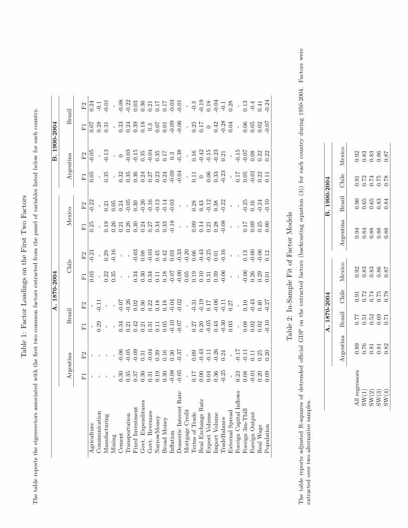
Tab

le1:

Fact

orLoa

ding

son

the

Fir

stT

wo

Fact

ors

The

table

report

sth

eei

gen

vec

tors

ass

oci

ate

dw

ith

the

firs

ttw

oco

mm

on

fact

ors

extr

act

edfr

om

the

panel

ofva

riable

slist

edbel

owfo

rea

chco

untr

y.

A.1870-2

004

B.1900-2

004

Arg

enti

na

Bra

zil

Chile

Mex

ico

Arg

enti

na

Bra

zil

F1

F2

F1

F2

F1

F2

F1

F2

F1

F2

F1

F2

Agri

cult

ure

--

--

0.0

3-0

.21

0.2

5-0

.22

0.0

5-0

.05

0.0

70.2

4C

om

munic

ati

on

--

0.2

9-0

.11

--

--

--

0.2

8-0

.1M

anufa

cturi

ng

--

--

0.2

20.2

90.1

90.2

10.3

5-0

.13

0.3

1-0

.01

Min

ing

--

--

0.3

5-0

.16

0.2

60.0

5-

--

-C

emen

t0.3

0-0

.06

0.3

4-0

.07

--

0.2

10.2

40.3

20

0.3

3-0

.08

Tra

nsp

ort

ati

on

0.3

5-0

.05

0.2

1-0

.26

--

0.2

6-0

.05

0.3

5-0

.03

0.2

4-0

.22

Fix

edIn

ves

tmen

t0.3

7-0

.09

0.4

20.0

20.3

4-0

.03

0.3

00.3

00.3

6-0

.15

0.3

90.0

3G

ovt.

Expen

dit

ure

s0.3

00.3

10.2

10.3

60.3

00.0

80.2

4-0

.26

0.2

40.3

50.1

80.3

6G

ovt.

Rev

enues

0.3

1-0

.04

0.3

10.2

20.3

4-0

.03

0.2

7-0

.16

0.2

7-0

.04

0.3

0.2

1N

arr

owM

oney

0.1

90.3

90.1

10.1

80.1

10.4

50.3

4-0

.13

0.2

30.3

50.0

70.1

7B

road

Money

0.3

00.1

60.0

50.1

80.1

80.4

20.3

3-0

.14

0.2

40.1

70.0

10.1

7In

flati

on

-0.0

80.3

0-0

.10

-0.0

4-0

.07

0.0

3-0

.18

-0.0

3-0

.09

0.3

-0.0

9-0

.03

Dom

esti

cIn

tere

stR

ate

-0.0

5-0

.37

-0.0

7-0

.02

-0.0

0-0

.33

--

-0.0

4-0

.38

-0.0

6-0

.01

Mort

gage

Cre

dit

--

--

0.0

5-0

.20

--

--

--

Ter

ms

ofTra

de

0.1

70.0

90.2

7-0

.31

0.1

90.0

60.0

90.2

80.1

10.1

60.2

5-0

.3R

ealE

xch

ange

Rate

0.0

0-0

.43

0.2

0-0

.19

0.1

0-0

.43

0.1

40.4

30

-0.4

20.1

7-0

.19

Export

Volu

me

0.0

4-0

.11

-0.0

50.1

70.3

1-0

.25

0.2

1-0

.12

0.0

6-0

.15

00.1

8Im

port

Volu

me

0.3

6-0

.26

0.4

3-0

.06

0.3

90.0

10.2

80.3

80.3

3-0

.23

0.4

2-0

.04

Tra

deB

ala

nce

-0.2

50.2

4-0

.30

-0.1

1-0

.06

-0.1

6-0

.08

-0.2

2-0

.23

0.2

1-0

.28

-0.1

Exte

rnalSpre

ad

--

0.0

30.2

7-

--

--

-0.0

40.2

8Fore

ign

Capit

alIn

flow

s0.2

3-0

.17

--

--

--

0.1

7-0

.15

--

Fore

ign

3m

-Tbill

0.0

8-0

.11

0.0

80.1

0-0

.06

0.1

30.1

7-0

.25

0.0

5-0

.07

0.0

60.1

3Fore

ign

Outp

ut

-0.0

10.1

10.0

2-0

.43

0.2

6-0

.00

0.0

90.1

6-0

.01

0.0

80.0

5-0

.4R

ealW

age

0.2

00.2

50.0

20.4

00.2

9-0

.06

0.2

5-0

.24

0.2

20.2

20.0

20.4

1Popula

tion

0.0

90.2

0-0

.10

-0.2

70.0

10.1

20.0

0-0

.10

0.1

10.2

2-0

.07

-0.2

4

Tab

le2:

In-S

ampl

eFit

ofFa

ctor

Mod

els

The

table

report

sadju

sted

R-s

quare

sof

det

rended

offi

cial

GD

Pon

the

extr

act

edfa

ctors

(back

cast

ing

equati

on

(3))

for

each

countr

yduri

ng

1950-2

004.

Fact

ors

wer

eex

tract

edov

ertw

oalt

ernati

ve

sam

ple

s.

A.1870-2

004

B.1900-2

004

Arg

enti

na

Bra

zil

Chile

Mex

ico

Arg

enti

na

Bra

zil

Chile

Mex

ico

All

regre

ssors

0.8

90.7

70.9

10.9

20.9

40.9

00.9

10.9

2SW

(1)

0.7

60.5

10.7

20.8

30.8

40.6

50.7

20.8

3SW

(2)

0.8

10.5

20.7

40.8

30.8

80.6

50.7

40.8

3SW

(3)

0.8

10.6

90.7

50.8

60.8

80.8

30.7

50.8

6SW

(4)

0.8

20.7

10.7

80.8

70.8

80.8

40.7

80.8

7

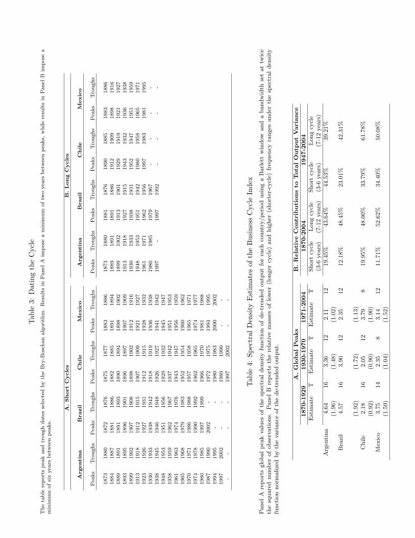
Tab

le3:

Dat

ing

the

Cyc

leT

he

table

report

spea

kand

trough

date

sse

lect

edby

the

Bry

-Bosc

han

alg

ori

thm

.R

esult

sin

Panel

Aim

pose

am

inim

um

oftw

oyea

rsbet

wee

npea

ks,

while

resu

lts

inPanel

Bim

pose

am

inim

um

ofsi

xyea

rsbet

wee

npea

ks.

A.Short

Cycle

sB

.Long

Cycle

s

Argentina

Brazil

Chile

Mexic

oA

rgenti

na

Brazil

Chile

Mexic

o

Pea

ks

Tro

ughs

Pea

ks

Tro

ughs

Pea

ks

Tro

ughs

Pea

ks

Tro

ughs

Pea

ks

Tro

ughs

Pea

ks

Tro

ughs

Pea

ks

Tro

ughs

Pea

ks

Tro

ughs

1873

1880

1872

1876

1875

1877

1883

1886

1873

1880

1881

1876

1890

1885

1883

1886

1884

1887

1881

1886

1882

1885

1891

1894

1889

1891

1891

1886

1912

1909

1898

1916

1889

1891

1891

1893

1890

1894

1898

1902

1899

1902

1913

1901

1929

1919

1921

1927

1893

1895

1896

1901

1896

1897

1907

1909

1913

1918

1927

1915

1943

1932

1936

1938

1899

1902

1907

1908

1898

1902

1912

1916

1930

1933

1938

1931

1952

1947

1951

1959

1913

1918

1912

1915

1907

1909

1921

1927

1948

1953

1951

1942

1980

1958

1965

1971

1923

1926

1927

1931

1912

1915

1928

1932

1961

1971

1962

1956

1997

1983

1981

1995

1930

1933

1938

1942

1918

1919

1936

1938

1980

1985

1979

1967

--

--

1938

1945

1946

1948

1926

1927

1941

1942

1997

-1997

1992

--

--

1948

1953

1951

1956

1929

1932

1945

1947

1958

1959

1962

1967

1937

1942

1951

1953

1961

1963

1974

1976

1943

1947

1956

1959

1965

1968

1979

1983

1952

1954

1960

1962

1970

1971

1986

1988

1957

1958

1965

1971

1974

1978

1990

1992

1962

1965

1974

1977

1980

1985

1997

1999

1966

1970

1981

1988

1987

1990

2002

-1972

1975

1994

1995

1994

1995

--

1980

1983

2000

2002

1997

2002

--

1989

1990

--

--

--

1997

2002

--

Tab

le4:

Spec

tral

Den

sity

Est

imat

esof

the

Bus

ines

sC

ycle

Inde

xPanel

Are

port

sglo

balpea

kva

lues

of

the

spec

tralden

sity

funct

ion

of

de-

tren

ded

outp

ut

for

each

countr

y/per

iod

usi

ng

aB

arl

ett

win

dow

and

abandw

idth

set

at

twic

eth

esq

uare

dnum

ber

of

obse

rvati

ons.

Panel

Bre

port

sth

ere

lati

ve

mass

esof

low

er(l

onger

cycl

e)and

hig

her

(short

er-c

ycl

e)fr

equen

cyra

nges

under

the

spec

tralden

sity

funct

ion

norm

alize

dby

the

vari

ance

ofth

ede-

tren

ded

outp

ut.

A.G

lobalPeaks

B.R

ela

tive

Contr

ibuti

ons

toTota

lO

utp

ut

Vari

ance

1870-1

929

1930-1

970

1971-2

004

1870-2

004

1947-2

004

Est

imate

TE

stim

ate

TE

stim

ate

TShort

cycl

eLong

cycl

eShort

cycl

eLong

cycl

e(3

-6yea

rs)

(7-1

2yea

rs)

(3-6

yea

rs)

(7-1

2yea

rs)

Arg

enti

na

4.6

416

3.3

612

2.1

112

19.4

5%

43.6

4%

44.5

3%

39.2

1%

(1.9

6)

(1.4

8)

(1.0

2)

Bra

zil

4.5

716

3.9

012

2.3

512

12.1

8%

48.4

5%

23.0

1%

42.3

1%

(1.9

2)

(1.7

2)

(1.1

3)

Chile

2.1

816

2.0

512

3.7

98

19.9

5%

48.0

0%

33.7

9%

61.7

8%

(0.9

2)

(0.9

0)

(1.9

0)

Mex

ico

3.7

514

2.3

58

3.1

412

11.7

1%

52.6

2%

34.4

0%

50.0

8%

(1.5

9)

(1.0

4)

(1.5

2)

Table 5: Disaggregated Persistence MeasuresThe table reports the values of P = (1 + θ1 + θp..)/(1− ρ1 − ..ρq) where θ and ρ are the moving average and auto-correlationcoefficients of an ARIMA (p,1,q) over the full period (1870-2004) and post-war sample (1947-2004).

A: 1870-2004

Argentina Brazil Chile Mexico LAC-4 Medianagriculture output 0.48 0.53 0.50 1.09 0.50manufacturing output 1.04 1.36 1.02 1.04 1.04mining output - - 0.71 1.65 0.71cement output 0.96 1.00 . 1.31 0.98transportation output 2.53 1.60 - 1.77 2.07communications output - 1.53 - - 1.53export volume 0.64 0.71 0.64 0.97 0.64import volume 0.96 1.12 1.11 0.88 1.11terms of trade 0.82 0.87 0.94 0.79 0.87fixed investment 1.30 1.15 0.93 1.19 1.15real gov. spending 0.85 0.88 0.76 1.14 0.85real gov. revenues 0.64 1.01 0.66 1.27 0.66real wage 0.91 1.05 0.84 1.00 0.91real exchange rate 0.47 0.44 0.70 0.81 0.47Mo/CPI 0.97 0.19 0.65 0.99 0.65M2/CPI 1.06 0.30 1.04 0.96 1.04real domestic interest rate 0.00 0.00 0.50 - 0.00Inflation 0.55 0.80 1.09 0.00 0.80Sovereign spread 0.36 0.33 1.00 - 0.36foreign capital flows 0.35 - - - 0.35foreign real GDP 1.41 1.41 1.41 1.31 1.41foreign real TB-bill rate 0.23 0.23 0.23 0.23 0.23Overall Median 0.73 0.80 0.84 0.97 0.80

B: 1947-2004

Argentina Brazil Chile Mexico LAC-4 Medianagriculture output 0.26 0.60 0.78 1.48 0.60manufacturing output 0.93 2.18 1.08 1.44 1.08mining output - - 0.93 1.24 0.93cement output 0.69 1.97 - 0.92 1.33transportation output 0.83 2.38 - 1.44 1.61communications output - 3.85 - - 3.85export volume 0.79 0.98 0.52 0.87 0.79import volume 0.79 1.17 0.94 0.87 0.94terms of trade 0.56 0.43 0.86 0.70 0.56fixed investment 0.77 1.07 1.06 0.94 1.06real gov. spending 0.49 0.91 1.02 1.04 0.91real gov. revenues 0.34 1.09 0.96 1.00 0.96real wage 0.80 1.60 0.43 1.38 0.80real exchange rate 0.25 0.37 0.89 0.23 0.37Mo/CPI 0.26 0.00 0.31 0.88 0.26M2/CPI 0.94 0.60 0.92 0.79 0.92real domestic interest rate 0.66 0.60 0.89 . 0.66Inflation 0.74 3.01 3.09 0.69 3.01Sovereign spread 1.05 0.45 0.74 0.44 0.74foreign capital flows 0.30 - - - 0.30foreign real GDP 1.26 1.26 1.26 1.03 1.26foreign real TB-bill rate 0.27 0.27 0.27 0.27 0.27Overall Median 0.71 1.03 0.91 0.92 0.92Real GDP Persistence 0.97 2.86 1.30 2.38 1.84

Tab

le6:

Per

sist

ence

and

Vol

atili

tyof

the

Cyc

leT

he

table

report

sauto

corr

elati

on

and

standard

dev

iation

estim

ate

sofour

new

busi

nes

scy

cle

indic

esin

Panel

A.Panel

Bre

port

sth

eco

rres

pondin

ges

tim

ate

softh

eH

P-fi

lter

eddet

rended

realG

DP

data

from

thes

eco

untr

ies’

nationalacc

ounts

.

A:B

ackcast

ed

Data

1870-1

929

1930-1

970

Arg

Bra

Chi

Mex

Arg

Bra

Chi

Mex

AR

(1)

0.7

28

0.7

27

0.6

40

0.7

67

0.6

17

0.6

16

0.5

54

0.5

73

Std

0.0

65

0.0

48

0.0

63

0.0

66

0.0

46

0.0

32

0.0

78

0.0

29

1971-1

987

1988-2

004

Arg

Bra

Chi

Mex

Arg

Bra

Chi

Mex

AR

(1)

0.0

59

0.6

59

0.6

14

0.6

54

0.5

79

0.4

82

0.5

62

0.4

72

Std

0.0

29

0.0

37

0.0

71

0.0

39

0.0

65

0.0

20

0.0

20

0.0

24

B:A

ctu

alG

DP

Data

1971-1

987

1988-2

004

Arg

Bra

Chi

Mex

Arg

Bra

Chi

Mex

AR

(1)

0.1

68

0.6

24

0.5

90

0.6

44

0.5

90

0.6

22

0.6

87

0.3

83

Std

0.0

34

0.0

43

0.0

81

0.0

39

0.0

68

0.0

21

0.0

33

0.0

30

Tab

le7:

Inte

rnat

iona

lC

ompa

riso

nson

Cyc

lical

Per

sist

ence

and

Vol

atili

tyT

he

table

com

pare

sauto

corr

elation

(AR

(1))

and

unco

ndit

ionalst

andard

dev

iation

(Std

)es

tim

ate

softh

enew

LA

C-4

busi

nes

scy

cle

indic

esw

ith

HP

-filter

det

rended

realG

DP

toth

ose

inoth

erco

untr

ies.

Panel

Ash

ow

sm

edia

nre

gio

nalvalu

esfo

rLA

C-4

,E

U-4

(Fra

nce

,G

erm

any,

Italy

and

the

UK

),N

W-3

(USA

,C

anada

and

Aust

ralia)

and

Japan

(JP

).Panel

Bin

cludes

abro

ad

LD

Cgro

up

(India

,In

dones

ia,K

ore

a,M

ala

ysi

a,Taiw

an,South

Afr

ica,and

Turk

ey),

as

wel

las

Afr

ica

(41

countr

ies)

,A

sia

(11

countr

ies)

,and

the

Mid

dle

East

(18

countr

ies)

usi

ng

Maddis

on

data

bef

ore

1950

and

offi

cialdata

ther

eaft

er.

A:A

dvanced

Countr

ies

1870-1

929

1930-1

970

LA

-4E

U-4

NW

-3JP

LA

-4E

U-4

NW

-3JP

AR

(1)

0.7

28

0.5

07

0.5

17

0.0

32

0.5

95

0.6

97

0.7

06

0.5

99

Std

0.0

64

0.0

51

0.0

50

0.0

35

0.0

39

0.1

01

0.0

66

0.1

28

1971-1

987

1988-2

004

LA

-4E

U-4

NW

-3JP

LA

-4E

U-4

NW

-3JP

AR

(1)

0.6

34

0.5

26

0.4

77

0.6

83

0.5

22

0.6

19

0.5

01

0.4

17

Std

0.0

38

0.0

17

0.0

21

0.0

27

0.0

22

0.0

15

0.0

22

0.0

18

B:D

evelo

pin

gC

ountr

ies

1930-1

950

1950-1

970

LA

-4O

ther

LD

Cs

Afr

ica

Asi

aM

iddle

East

LA

-4O

ther

LD

Cs

Afr

ica

Asi

aM

iddle

East

AR

(1)

0.5

60

0.6

17

--

-0.2

73

0.0

51

0.5

02

0.4

16

0.4

02

Std

0.0

40

0.0

78

--

-0.0

31

0.0

30

0.0

38

0.0

28

0.0

43

1971-1

987

1988-2

004

LA

-4O

ther

LD

Cs

Afr

ica

Asi

aM

iddle

East

LA

-4O

ther

LD

Cs

Afr

ica

Asi

aM

iddle

East

AR

(1)

0.6

07

0.5

51

0.5

63

0.4

86

0.4

47

0.6

06

0.5

31

0.4

81

0.5

47

0.5

72

Std

0.0

41

0.0

38

0.0

51

0.0

33

0.0

31

0.0

31

0.0

28

0.0

35

0.0

28

0.0

57

Tab

le8:

Dis

aggr

egat

edM

easu

res

ofC

yclic

alV

olat

ility

The

table

report

sst

andard

dev

iati

ons

(in

per

cent)

for

sele

cted

vari

able

sand

diff

eren

tsa

mple

per

iods.

Monet

ary

vari

able

sare

expre

ssed

inre

alte

rms

(CP

Idefl

ate

d).

All

vari

able

sare

mea

sure

das

dev

iati

ons

from

thei

rH

P-fi

lter

edtr

ends

wit

hth

eex

ception

ofex

pen

diture

tore

ven

ue

ratios

and

realin

tere

stra

tes.

1870-1

929

1930-1

970

1971-2

004

Arg

enti

na

Bra

zil

Chile

Mex

ico

Arg

enti

na

Bra

zil

Chile

Mex

ico

Arg

enti

na

Bra

zil

Chile

Mex

ico

Fore

ign

Inte

rest

Rate

5.3

45.3

45.3

45.3

44.6

84.6

84.6

84.6

82.2

02.2

02.2

02.2

0Fore

ign

Outp

ut

3.4

63.4

63.4

63.4

67.0

87.0

87.0

87.0

82.9

72.9

72.9

72.9

7D

om

esti

cO

utp

ut

6.4

94.8

46.2

57.2

94.5

63.2

57.6

92.9

05.0

12.9

45.3

53.3

0Ter

ms

ofTra

de

14.9

921.7

933.0

529.0

012.2

020.2

726.6

629.3

727.1

412.2

416.4

522.2

0E

xport

Volu

me

13.2

010.2

117.6

110.3

413.5

99.9

516.8

99.5

212.9

48.1

16.8

79.6

1Fix

edIn

ves

tmen

t45.3

034.9

630.4

534.0

420.7

829.5

634.6

713.4

316.6

415.3

220.9

414.7

0G

over

nm

ent

Spen

din

g14.7

910.5

115.8

812.8

811.4

313.8

214.0

58.5

311.7

610.3

39.4

410.5

8E

xpen

diture

/R

even

ue

28.4

120.8

228.8

310.7

023.3

616.2

113.8

319.6

422.5

39.0

512.1

518.0

5N

arr

ow

Money

14.9

415.3

216.6

435.0

710.2

011.0

119.9

015.4

316.8

415.8

121.8

910.4

8B

road

Money

14.8

214.6

211.3

935.8

312.3

310.8

413.4

613.6

220.3

222.8

217.3

119.0

0R

ealW

age

12.3

39.1

48.6

932.7

36.9

96.5

413.0

718.2

212.4

45.7

212.3

015.1

3

Tab

le9:

Sync

hron

izat

ion

ofth

eLat

inA

mer

ican

Cyc

les

The

table

report

sth

eH

ard

ing-P

agan

(2002)

conco

rdance

statist

ic.

Valu

escl

ose

toone

show

evid

ence

ofa

stro

nger

deg

ree

ofsy

nch

ronic

ity.

1878-1

929

1930-1

970

Arg

Bra

Chi

Mex

Arg

Bra

Chi

Mex

Arg

1.0

00.4

80.5

40.6

21.0

00.5

40.5

40.4

9B

ra-

1.0

00.7

90.7

1-

1.0

00.6

60.4

6C

hi

--

1.0

00.7

7-

-1.0

00.6

1M

ex-

--

1.0

0-

--

1.0

01971-1

987

1988-2

004

Arg

Bra

Chi

Mex

Arg

Bra

Chi

Mex

Arg

1.0

00.5

90.5

30.7

61.0

00.4

10.8

20.7

1B

ra-

1.0

00.7

10.5

9-

1.0

00.4

70.4

7C

hi

--

1.0

00.4

1-

-1.0

00.6

5M

ex-

--

1.0

0-

--

1.0

0

Tab

le10

:In

divi

dual

Cou

ntry

Cor

rela

tion

sw

ith

the

Reg

iona

lC

omm

onFa

ctor

The

table

report

sco

rrel

ation

coeffi

cien

tsof

the

regio

nalco

mm

on

fact

ors

with

the

resp

ective

countr

y-s

pec

ific

counte

rpart

s.T

he

regio

nalco

mm

on

fact

ors

wer

eex

tract

edby

pooling

all

indiv

idualco

untr

yse

ries

toget

her

and

usi

ng

pri

nci

palco

mponen

tsfa

ctor

analy

sis.

1878-1

929

1930-1

970

1971-1

987

1988-2

004

Reg

ionalF1

Reg

ionalF2

Reg

ionalF1

Reg

ionalF2

Reg

ionalF1

Reg

ionalF2

Reg

ionalF1

Reg

ionalF2

Arg

enti

na

0.6

80.5

10.5

6-0

.07

0.2

90.7

90.8

00.3

1B

razi

l0.8

00.1

80.6

6-0

.40

0.6

30.3

00.6

00.2

7C

hile

0.7

00.5

50.8

20.5

60.8

40.5

70.7

4-0

.44

Mex

ico

0.8

60.0

60.7

5-0

.06

0.8

30.6

00.4

30.4

1M

edia

n0.7

50.3

50.7

1-0

.07

0.7

30.5

90.6

70.2

9

Tab

le11

:SU

RE

Reg

ress

ions

ofD

omes

tic

Cyc

les

onG

loba

lFa

ctor

s

The

tabl

ere

port

sSU

RE

regr

essi

ons

ofgl

obal

vari

able

son

the

busi

ness

cycl

ein

dex

(dom

esti

ccy

cle)

for

each

coun

try.

Cou

ntry

indi

ces

wer

eex

trac

ted

from

the

pane

lofv

aria

bles

inTab

le1,

excl

udin

gth

efo

reig

nin

tere

stra

tean

dou

tput

vari

able

s.t-

stat

isti

csar

ere

port

edin

pare

nthe

ses.

A.B

asel

ine

Spec

ifica

tion

B.In

cludin

gLA

cris

isD

um

my

Arg

enti

naB

razi

lC

hile

Mex

ico

Arg

enti

naB

razi

lC

hile

Mex

ico

Wor

ldO

utpu

t0.

100

0.15

00.

583

0.15

00.

050

0.15

20.

520

0.14

0(1

.23)

(2.7

7)(6

.35)

(3.5

8)(0

.68)

(2.7

7)(5

.90)

(3.3

0)W

orld

real

inte

rest

rate

-0.1

60-0

.140

-0.2

30-0

.010

-0.1

50-0

.140

-0.2

10-0

.010

(-1.

93)

(2.4

1)(2

.58)

(-0.

35)

(-1.

95)

(-2.

42)

(-2.

56)

(-0.

38)

Wor

ldco

mm

odity

TO

T0.

006

0.00

20.

015

0.01

7-0

.003

0.00

20.

006

0.01

4(0

.48)

(0.2

2)(1

.09)

(1.8

7)(-

0.32

)(0

.24)

(0.4

5)(1

.49)

Wor

ldW

ardu

mm

y-0

.070

-0.0

54-0

.059

-0.0

53-0

.068

-0.0

54-0

.059

-0.0

55(-

4.51

)(-

4.88

)(-

3.59

)(-

4.94

)(-

4.83

)(-

4.90

)(-

3.71

)(-

5.01

)LA

cris

esdu

mm

y-

--

--0

.056

-0.0

01-0

.047

-0.0

20-

--

-(5

.18)

(-0.

1)(-

3.81

)(-

2.34

)Lag

ged

cycl

e(t-

1)0.

610

0.74

00.

600

0.93

00.

670

0.73

00.

610

0.93

0(9

.74)

(8.8

3)(8

.24)

(12.

96)

(11.

44)

(8.7

6)(8

.65)

(13.

22)

Lag

ged

cycl

e(t

-2)

--0

.160

-0.3

09-0

.478

--0

.150

-0.2

60-0

.460

-(-

1.90

)(-

4.55

)(-

6.90

)-

(-1.

87)

(-3.

77)

(-6.

74)

Obs

erva

tion

s12

512

512

512

512

512

512

512

5R

20.

520.

610.

580.

710.

60.

610.

630.

73

Co-

vari

ance

Mat

rix

ofR

esid

uals

:C

o-va

rian

ceM

atri

xof

Res

idua

ls:

Arg

enti

na1

1B

razi

l-0

.04

1.00

-0.0

51.

00C

hile

0.25

0.06

1.00

0.10

0.08

1.00

Mex

ico

0.10

0.10

0.22

10.

020.

100.

191.

00

Bre

usch

-Pag

ante

stof

inde

pend

ence

:ch

i2(6

)=

17.3

2,P

r=

0.01

Bre

usch

-Pag

ante

stof

inde

pend

ence

:ch

i2(6

)=

8.21

,P

r=

0.22

Oth

erst

atis

tics

:R

2ex

c.fo

reig

nse

ries

0.42

0.53

0.45

0.64

R2

glob

alfa

ctor

son

ly0.

140.

250.

40.

44R

2gl

obal

&D

cris

ison

ly0.

180.

260.

440.

45

Table 12: External Determinants of the Common Latin American Cycle

This table reports OLS regressions of the common component LAC-4 regional factor (F1) on short-term (3-month Treasury bills) interest rates deflated by CPI inflation and the weighted real GDPcycle in the G-8 advanced countries (G-7 advanced economies plus Australia). All regressionsinclude an intercept. Panel B adds the logarithm of a global index of the US$ price of commoditiesrelative to manufacturing. t-statistics are reported in parentheses.

A: World Commodity Prices Excluded

1880-1929 1930-1970 1971-2004Foreign Real Interest Rate -0.19 -0.20 -0.23

(-2.47) (-3.75) (-1.87)Foreign Output 0.23 0.12 0.42

(2.71) (2.43) (2.50)World War Dummy -0.07 -0.04 -

(-6.31) (-3.2) -Lagged cycle(t-1) 0.68 0.80 0.77

(7.57) (6.86) (6.92)Lagged cycle(t-2) - -0.45 -

- (-3.85) -

R2 all 0.82 0.78 0.67R2 exc. lagged cycle 0.65 0.57 0.34DW 1.26 2.08 1.63Observations 50 41 34

B: World Commodity Prices Included

1880-1929 1930-1970 1971-2004Foreign Real Interest Rate -0.22 -0.14 -0.22

(-1.93) (-2.13) (-1.88)Foreign Output 0.23 0.11 0.43

(2.72) (2.33) (2.58)World Commodity TOT -0.02 0.04 0.06

(-0.47) (1.91) (-0.67)World War Dummy -0.07 -0.03 -

(-5.67) (-3.1) -Lagged cycle(t-1) 0.70 0.79 0.79

(7.34) (6.96) (6.81)Lagged cycle(t-2) - -0.44 -

- (-4.17) -

R2 all 0.82 0.80 0.68R2 exc. lagged cycle 0.69 0.59 0.39DW 1.47 2.04 1.72Observations 50 41 34

Fig

ure

1:C

omm

onFa

ctor

s

Com

pari

son

ofth

efir

sttw

oco

mm

onfa

ctor

s(F

1,F2)

extr

acte

dfr

omse

ries

detr

ende

dw

ith

the

Hod

rick

-Pre

scot

t(H

P),

and

the

Bax

ter-

Kin

g(B

K)

filte

rs.

1880

1900

1920

1940

1960

1980

2000

−505

Arg

entin

a: F

1

HP

BK

1880

1900

1920

1940

1960

1980

2000

−10−

505

Arg

entin

a: F

2

1880

1900

1920

1940

1960

1980

2000

−505

Bra

zil:

F1

HP

BK

1880

1900

1920

1940

1960

1980

2000

−505

Bra

zil:

F2

1880

1900

1920

1940

1960

1980

2000

−10−

505

Chi

le: F

1

HP

BK

1880

1900

1920

1940

1960

1980

2000

−505

Chi

le: F

2

1880

1900

1920

1940

1960

1980

2000

−10−

505

Mex

ico:

F1

HP

BK

1880

1900

1920

1940

1960

1980

2000

−505

Mex

ico:

F2

Fig

ure

2:A

ctua

lan

dB

ackc

aste

dV

alue

sof

Cyc

lical

Gro

wth

Com

pari

son

betw

een

back

cast

edva

lues

,pre

viou

ses

tim

ates

and

nati

onal

inco

me

acco

unts

data

for

Arg

enti

na,B

razi

l,C

hile

,and

Mex

ico.

All

reg.

deno

tes

back

cast

edva

lues

that

use

allav

aila

ble

regr

esso

rs.

The

seri

esSW

(r)

deno

tes

our

new

busi

ness

cycl

ein

dex

extr

acte

dus

ing

the

Stoc

kan

dW

atso

n(S

W)

appr

oach

wit

hr

stat

icfa

ctor

s.

1870

1880

1890

1900

1910

1920

1930

1940

1950

−0.

15

−0.

1

−0.

050

0.050.

1

0.15

Arg

entin

a, S

ampl

e 18

70−

1950

Pre

viou

sA

ll re

g.S

W(2

)

1950

1955

1960

1965

1970

1975

1980

1985

1990

1995

2000

−0.

15

−0.

1

−0.

050

0.050.

1

0.15

Arg

entin

a, S

ampl

e 19

50−

2004

Nat

. acc

.A

ll re

g.S

W(2

)

1870

1880

1890

1900

1910

1920

1930

1940

1950

−0.

1

−0.

050

0.050.

1

Bra

zil,

Sam

ple

1870

−19

50

Pre

viou

sA

ll re

g.S

W(3

)

1950

1955

1960

1965

1970

1975

1980

1985

1990

1995

2000

−0.

1

−0.

050

0.050.

1

Bra

zil,

Sam

ple

1950

−20

04

Nat

. acc

.A

ll re

g.S

W(3

)

1870

1880

1890

1900

1910

1920

1930

1940

1950

−0.

3

−0.

2

−0.

10

0.1

0.2

Chi

le, S

ampl

e 18

70−

1950

Pre

viou

sA

ll re

g.S

W(2

)

1950

1955

1960

1965

1970

1975

1980

1985

1990

1995

2000

−0.

3

−0.

2

−0.

10

0.1

0.2

Chi

le, S

ampl

e 19

50−

2004

Nat

. acc

.A

ll re

g.S

W(2

)

1880

1890

1900

1910

1920

1930

1940

1950

−0.

3

−0.

25

−0.

2

−0.

15

−0.

1

−0.

050

0.050.

1

Mex

ico,

Sam

ple

1878

−19

50

Pre

viou

sA

ll re

g.S

W(2

)

1950

1955

1960

1965

1970

1975

1980

1985

1990

1995

2000

−0.

3

−0.

25

−0.

2

−0.

15

−0.

1

−0.

050

0.050.

1

Mex

ico,

Sam

ple

1950

−20

04

Nat

. acc

.A

ll re

g.S

W(2

)

Figure 3: Recursive Parameter Estimates

Recursive estimates of the coefficients in backcasting regression(3). c is the intercept of that regression while b1,b2,

and b3 are the slope coefficients for the first three common factors.

1920 1930 1940 1950 1960−0.01

0

0.01

0.02

0.03Argentina

c

b1

b2

1920 1930 1940 1950 1960−0.01

0

0.01

0.02

0.03Brazil

c

b1

b2

b3

1940 1945 1950 1955 1960−0.01

0

0.01

0.02

0.03

Chile

c

b1

b2

1925 1930 1935 1940 1945 1950 1955 1960−0.01

0

0.01

0.02

0.03Mexico

c

b1

b2

Figure 4: Volatility

The figure reports 10-Year rolling window estimates of standard deviations of the backcasted business cycle. The top

panel reports estimates for Argentina, Brazil, Chile, and Mexico. The backcasted values are based on a model using

two common static factors (three for Brazil). The bottom panel reports estimates for the LAC-4 region.

1880 1900 1920 1940 1960 1980 20000

0.05

0.1

0.15

0.2Rolling Standard Deviation of Backcasted Cycles

ArgBraChiMex

1880 1900 1920 1940 1960 1980 20000

0.02

0.04

0.06

0.08

0.1Rolling Standard Deviation of Backcasted LAC−4 Cycle

LAC4

Fig

ure

5:H

isto

rica

lE

vent

Cha

rts

The

pane

lsre

port

the

back

cast

edbu

sine

sscy

cle

for

Arg

enti

na,B

razi

l,C

hile

and

Mex

ico

agai

nst

wor

ldec

onom

icev

ents

(dar

ksh

aded

area

)an

dco

untr

y-sp

ecifi

cev

ents

(lig

htsh

aded

area

).

A:18

70-1

949

1870

1880

1890

1900

1910

1920

1930

1940

−0.

10

0.1

↓Wor

ld S

tock

Mar

ket C

rash

Eu

Ban

king

Cris

is→

←B

arin

g C

risis Fin

anci

al P

anic

→

←W

WI

Gre

at D

epre

ssio

n→

WW

II→

←E

xits

Gol

d

← R

ejoi

ns G

old

Argentina

1870

1880

1890

1900

1910

1920

1930

1940

−0.

10

0.1

↓Wor

ld S

tock

Mar

ket C

rash

Fin

anci

al P

anic

↓↓G

reat

Dep

ress

ion

↓Enc

ilham

ento

←D

ebt R

esch

edul

ing

Join

s G

old→

↓Def

ault/

Exi

ts G

old

Rej

oins

Gol

d→

Brazil

Eu

Ban

king

Cris

is→

←W

WI

WW

II→←

WW

I

1870

1880

1890

1900

1910

1920

1930

1940

−0.

3−

0.2

−0.

100.

1

↓Wor

ld S

tock

Mar

ket C

rash ←

Eu

Ban

king

Cris

is

↓Fin

anci

al P

anic

War

of t

he

Pac

ific→

←G

old

Sta

ndar

d

Chile

←W

WI

Gre

at D

epre

ssio

n→

WW

II→

1870

1880

1890

1900

1910

1920

1930

1940

−0.

3

−0.

2

−0.

10

0.1

Fin

anci

al P

anic

↓↓G

reat

Dep

ress

ion

←W

WII

Dia

z’s

dict

ator

ship

↓↓D

ubla

n’s

aust

erity

pla

n

←F

orei

gn D

ebt C

onve

rsio

nJoin

s G

old→

↓ R

evol

utio

n↓

hype

rinfla

tion

Mexico

Eu

Ban

king

Cris

is→

←W

WI

B:19

50-2

004

1950

1955

1960

1965

1970

1975

1980

1985

1990

1995

2000

−0.

15

−0.

1

−0.

050

0.05

←K

orea

War

Firs

t Oil

Sho

ck→

Sec

ond

O

il S

hock

→

Asi

a−

R

ussi

a

C

risis

→

↓US

sto

ck m

arke

t Cra

sh

↓Sov

erei

gn D

efau

lt

Hyp

erin

flatio

n→

Con

vert

ibili

ty P

lan↓

Teq

uila

Cris

is→

Bra

Cur

renc

y C

risis

↓

Argentina

Mili

tary

Cou

p↓

←D

ebt

Cris

is

Wal

l Str

eet

C

rash

→

1950

1955

1960

1965

1970

1975

1980

1985

1990

1995

2000

−0.

04

−0.

020

0.02

↓Sov

erei

gn D

efau

lt

Mili

tary

Cou

p→

Col

or Im

peac

hmen

t↓C

urre

ncy

Cris

is↓

Brazil

←K

orea

War

Firs

t Oil

Sho

ck→

Sec

ond

O

il S

hock

→

Wal

l Str

eet

C

rash

→

←D

ebt

Cris

is

Hyp

erin

flatio

n→H

yper

infla

tion→

Asi

a−

R

ussi

a

C

risis

→

1950

1955

1960

1965

1970

1975

1980

1985

1990

1995

2000

−0.

1

−0.

050

0.05

←D

ebt

Cris

is

Asi

a−R

ussi

a C

risis

→

US

sto

ck m

arke

t Cra

sh↓

↓Sov

erei

gn D

efau

ltM

ilita

ry C

oup↓

Chile

←K

orea

War

Firs

t Oil

Sho

ck→

Sec

ond

O

il S

hock

→←

Wal

l Str

eet

C

rash

1950

1955

1960

1965

1970

1975

1980

1985

1990

1995

2000

−0.

050

0.050.

1D

ebt C

risis

↓

Wal

l Str

eet

C

rash

→

Asi

a−R

ussi

a C

risis

↓↓S

over

eign

Def

ault

NA

FT

A n

egot

iatio

ns↓

Mexico

←K

orea

War

Firs

t Oil

Sho

ck→

Sec

ond

O

il S

hock

→

Teq

uila

Cris

is→