ABSTRACT

Title of Document: TRACING SULFUR SOURCES IN AN

ARCHEAN HYDROTHERMAL SYSTEM USING SULFUR MULTIPLE ISOTOPES – A CASE STUDY FROM THE KIDD CREEK VOLCANOGENIC MASSIVE SULFIDE DEPOSIT

John William Jamieson, M.S., 2005 Directed By: Professor James Farquhar

Department of Geology Mass-independent fractionation of sulfur isotopes in the Archean atmosphere resulted

in surface sulfur reservoirs with distinct isotopic signatures. These signatures are

used to trace the movement of sulfur through an Archean seafloor hydrothermal

system associated with the Kidd Creek volcanogenic massive sulfide (VMS) deposit.

Isotopic measurements of sulfides from the 2.7 Ga Kidd Creek VMS deposit reflect

two separate sulfur sources for ore precipitation. Subseafloor ore has a

predominantly juvenile sulfur source. with a small (~3%) component of seawater

sulfate, which was transported through the hydrothermal system to the site of

precipitation. Surface sulfides contain a significant proportion of sulfur that was

stripped from coeval seawater sulfate or native sulfur at the site of precipitation.

Mass-independent isotopic signatures are also used in a sulfur multiple-isotope

framework to evaluate isotopic disequilibrium and to assess the suitability of mineral

pairs for paleothermometric calculations in the Kidd Creek VMS deposit.

TRACING SULFUR SOURCES IN AN ARCHEAN HYDROTHERMAL SYSTEM USING SULFUR MULTIPLE ISOTOPES – A CASE STUDY FROM THE KIDD

CREEK VOLCANOGENIC MASSIVE SULFIDE DEPOSIT

By

John William Jamieson

Thesis submitted to the Faculty of the Graduate School of the University of Maryland, College Park, in partial fulfillment

of the requirements for the degree of Master of Science

2005 Advisory Committee: Professor James Farquhar, Chair Professor Philip A. Candela Professor A. Jay Kaufman

Acknowledgements

I would like to thank James Farquhar for giving me the opportunity to come to

Maryland and allowing me to pursue such interesting research topics. This thesis has

benefited immensely from his wisdom and open mind. I would like to thank Boswell

Wing for his guiding hand throughout this project. Without his scientific, technical

and moral support, the potential of this research would not have been realized. Daily

laboratory discussions with James, Boz, and David Johnston, together with their

infinite sense of humor, made working in the lab a pleasure. Discussions with Mark

Hannington and Ian Jonasson greatly improved my understanding of the geology of

the Kidd Creek region. Comments and suggestions by Philip Candela and Jay

Kaufman have enhanced the quality of this thesis.

Finally, I would like to especially thank Anetta Banas for her endless love, emotional

support and scientific insights, all of which have kept me close to home.

This research was supported by an NSERC Post-Graduate Scholarship to J.W.

Jamieson, NSF grants EAR-0348382 and EAR-0003419 to J. Farquhar, and NASA

Exobiology grant NAG-512350 to J. Farquhar and B.A. Wing.

ii

Table of Contents Acknowledgements....................................................................................................... ii Table of Contents......................................................................................................... iii List of Tables ............................................................................................................... iv List of Figures ............................................................................................................... v Chapter 1: Introduction ................................................................................................. 1

1.1 Overview............................................................................................................ 1 1.2 Mass-independent Fractionation........................................................................ 1 1.3 Archean Sulfur Cycle......................................................................................... 4 1.4 Applications for Terrestrial Systems ................................................................. 8 1.5 Ore-forming Processes in Volcanogenic Massive Sulfide (VMS) Deposits ... 10 1.6 Accomplishments of this Thesis ...................................................................... 12

Chapter 2: Geological Background and Previous Work............................................. 15 2.1 The Kidd Creek Volcanogenic Massive Sulfide Deposit ................................ 15 2.2 Previous Sulfur-isotope Studies of Kidd Creek ............................................... 20

Chapter 3: Methods..................................................................................................... 22 3.1 Sulfur Isotope Measurements .......................................................................... 22 3.2 Interpretational Framework ............................................................................. 23 3.3 Analytical Uncertainties................................................................................... 24

Chapter 4: Results ....................................................................................................... 27 4.1 Kidd Creek Sulfides......................................................................................... 27 4.2 Sulfide Mineral Pairs ....................................................................................... 33

Chapter 5: Discussion ................................................................................................ 35 5.1 Sources of Sulfur at Kidd Creek ...................................................................... 35 5.2 Isotopic Disequilibrium in Sulfide Mineral Pairs ............................................ 41

Chapter 6: Conclusions .............................................................................................. 47 Appendix..................................................................................................................... 50 Bibliography ............................................................................................................... 52

iii

List of Tables Page

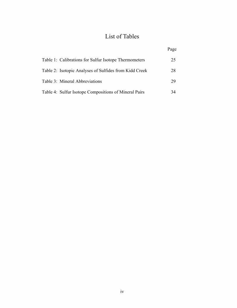
Table 1: Calibrations for Sulfur Isotope Thermometers 25

Table 2: Isotopic Analyses of Sulfides from Kidd Creek 28

Table 3: Mineral Abbreviations 29 Table 4: Sulfur Isotope Compositions of Mineral Pairs 34

iv

List of Figures

Figure 1: δ33S vs. δ34S plot of terrestrial, mass-dependent sulfur-bearing compounds younger than 2.0 Ga 3

Figure 2: ∆33S of terrestrial sulfur compounds versus time 5 Figure 3: Conceptual diagram of the Archean sulfur cycle 6 Figure 4: Cross-section of a seafloor hydrothermal system 13 Figure 5: Cross-section (reconstructed) of Kidd Creek 17 Figure 6: Representative ore textures from Kidd Creek 19 Figure 7: Traditional three-isotope plot of sulfides from Kidd Creek 30 Figure 8: ∆33S vs. δ34S plot of Kidd Creek sulfides 31 Figure 9: Conceptual diagram of surface sulfur reservoirs associated

with seafloor hydrothermal circulation 40 Figure 10: Mineral isotopic composition during precipitation and

equilibration 43 Figure 11: Sulfur multiple-isotope measurements for mineral pairs

from Kidd Creek 45

v

Chapter 1: Introduction

1.1 Overview

Reports of mass-independent sulfur isotope signatures in Archean sedimentary

rocks (Farquhar et al., 2000; 2001) have yielded significant new insights into the

Earth’s early sulfur cycle and its ties to the chemistry of the Archean atmosphere.

The results of the research by Farquhar et al. (2000; 2001) have raised a number of

questions about the size of Archean geochemical reservoirs and the vigor of exchange

between them. One of the most poorly understood of these reservoirs is that of

oceanic sulfate. Sulfate in Archean oceans is thought to have had a unique and

characteristic mass-independent sulfur isotope signatures, and recent work (Wing et

al., 2002) indicates that this signature is transferred to sulfide minerals in several

Archean VMS (Volcanogenic Massive Sulfide) deposits in the Superior Province of

Canada. Here, I focus on the Archean VMS deposit, Kidd Creek, located near

Timmins, Ontario, to study the nature of the oceanic sulfate reservoir, and to extract

new information about the nature of the hydrothermal systems and processes that

operated during formation of Archean VMS deposits.

1.2 Mass-independent Fractionation

Sulfur isotope analyses are reported as δ values, which for 34S and 32S, are defined as:

δ34SSample =34 RSample

34 RV−CDT

−1⎛

⎝ ⎜

⎞

⎠ ⎟ ×1000 , (1.1)

1

where 34R is the ratio of the abundance of 34S to abundance of 32S, and the V-CDT

subscript indicates the reference scale defined by the isotopic composition of the

international standard Ag2S, IAEA-S1. This standard has a defined isotopic

composition of δ34S ≡ -0.3 ‰ V-CDT (Krouse and Coplen, 1997). Samples were

measured relative to a laboratory standard SF6 gas. This gas has a known

composition, relative to the IAEA-S1 standard, based on multiple repeat

measurements. For this study, we took IAEA-S1 to have δ33S = -0.05 per mil V-CDT

(Gao and Thiemens, 1993), which assumes concordance between the CDT and V-

CDT scales.

Isotope effects that accompany most chemical and physical processes are

controlled by the relative difference in mass of the isotopes. Variations of δ33S values

are usually about half the coincident variations in δ34S values and reflect the fact that

δ33S is a measure of changes in 33S/32S (1 a.m.u difference) and δ34S is a measure of

changes in 34S/32S (2 a.m.u. difference). This mass dependence of sulfur isotope

fractionation produces a highly-correlated array on a plot of δ33S versus δ34S values

for most terrestrial sulfur-bearing materials (Fig. 1). Theoretical calculations, based

on equilibrium isotope partitioning, indicate that this array should be described by

δ33S =δ34 S1000

+1⎛

⎝ ⎜

⎞

⎠ ⎟

λ

−1⎡

⎣ ⎢ ⎢

⎤

⎦ ⎥ ⎥ ×1000, (1.2)

with λ = 0.515 (+0.003/-0.002) (Hulston and Thode, 1965). Sulfur-bearing terrestrial

samples that are older than ~2.45 Ga have been shown to possess sulfur multiple-

isotope compositions that, in some cases, fall far outside the limits allowed by mass-

dependent variations in λ (e.g., Farquhar et al., 2000). Precisely how a sample’s

2

Figure 1: δ33S vs. δ34S plot of terrestrial, mass-dependent sulfur-bearing compounds younger than 2.0 Ga. The black line represents the Terrestrial Fractionation Line (TFL). The slope of this line (~0.5) reflects the 1 a.m.u difference recorded by δ33S, relative to the 2 a.m.u. difference recorded by δ34S. Sulfur-bearing samples that have experience mass-independent fractionation will plot above or below the TFL.

3

sulfur multiple-isotope composition deviates from a reference mass-dependent

fractionation array can be quantified by the following relationship:

1000111000

SSSRFL34

3333 ×⎥⎥⎦

⎤

⎢⎢⎣

⎡−⎟⎟

⎠

⎞⎜⎜⎝

⎛+−=∆

λδδ , (1.3)

where λRFL (Reference Fractionation Line) ≡ 0.515 (Hulston and Thode, 1965). This

formulation removes much of the mass-dependent correlation that is inherent in the

fractionation due to most chemical and physical isotope effects, and provides a

measure to describe deviations from the RFL. In essence, it transforms δ33S values

into a new coordinate space where the exponential curve described by (1.2) is parallel

to the δ34S axis.

1.3 Archean Sulfur Cycle

Mass-independent fractionation of sulfur isotopes is recorded in natural

samples older than 2.45 Ga (Fig. 2) (Farquhar et al., 2000; Farquhar and Wing,

2003;Mojzsis et al., 2003; Ono et al., 2003; Bekker et al., 2004). Samples that are

younger than 2.0 Ga have ∆33S values indicating no significant mass-independent

fractionation. This shift in isotope fractionation mechanisms and/or preservation of

isotope ratios in the rock record indicates a fundamental change in sulfur chemistry

and/or cycling through the Earth system in the Neoarchean. The only experimentally

verified mechanism for producing substantial non-zero ∆33S values is through

photochemistry of sulfur-bearing gas phase compounds (Thiemens, 1999; Farquhar et

al., 2000; 2001).

4

Figure 2: Plot of ∆33S of terrestrial sulfur compounds versus time, showing mass-independent fractionation in samples older than 2.45 Ga. The green zone surrounding the x-axis indicates the deviations from the TFL that are permissible for mass-dependent processes. (Sources: Farquhar et al.; 2000, Mojzsis et al., 2003; Ono et al., 2003; Hu et al., 2003;Bekker et al., 2004; unpublished data from this lab)

5

Figure 3: Conceptual diagram of the Archean sulfur cycle, showing the movement of various sulfur species between reservoirs and their associated ∆33S values. Juvenile sulfur is erupted in to the atmosphere with an initial ∆33S of 0‰. Photochemical reactions in the atmosphere impart non-zero ∆33S values on intermediate sulfur species, which ultimately return to the surface in a soluble oxidized form (sulfate) and insoluble reduced form (S8 aerosol), with negative and positive ∆33S values, respectively. Modified from Farquhar and Wing (2003).

6

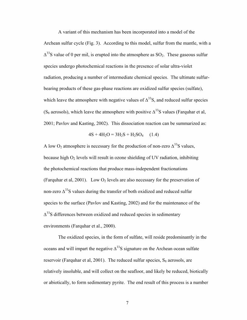
A variant of this mechanism has been incorporated into a model of the

Archean sulfur cycle (Fig. 3). According to this model, sulfur from the mantle, with a

∆33S value of 0 per mil, is erupted into the atmosphere as SO2. These gaseous sulfur

species undergo photochemical reactions in the presence of solar ultra-violet

radiation, producing a number of intermediate chemical species. The ultimate sulfur-

bearing products of these gas-phase reactions are oxidized sulfur species (sulfate),

which leave the atmosphere with negative values of ∆33S, and reduced sulfur species

(S8 aerosols), which leave the atmosphere with positive ∆33S values (Farquhar et al,

2001; Pavlov and Kasting, 2002). This dissociation reaction can be summarized as:

4S + 4H2O = 3H2S + H2SO4 (1.4)

A low O2 atmosphere is necessary for the production of non-zero ∆33S values,

because high O2 levels will result in ozone shielding of UV radiation, inhibiting

the photochemical reactions that produce mass-independent fractionations

(Farquhar et al, 2001). Low O2 levels are also necessary for the preservation of

non-zero ∆33S values during the transfer of both oxidized and reduced sulfur

species to the surface (Pavlov and Kasting, 2002) and for the maintenance of the

∆33S differences between oxidized and reduced species in sedimentary

environments (Farquhar et al., 2000).

The oxidized species, in the form of sulfate, will reside predominantly in the

oceans and will impart the negative ∆33S signature on the Archean ocean sulfate

reservoir (Farquhar et al, 2001). The reduced sulfur species, S8 aerosols, are

relatively insoluble, and will collect on the seafloor, and likely be reduced, biotically

or abiotically, to form sedimentary pyrite. The end result of this process is a number

7

of Archean sulfur reservoirs with distinct ∆33S compositions that can be used as a

chemically-conservative tracer of sulfur transfer through Archean geological

environments (Farquhar et al., 2002; Farquhar and Wing, 2003).

1.4 Applications for Terrestrial Systems

Stable isotope ratios, recorded in the rock record, have been used extensively

in investigations of paleoenvironments, and the evolution of terrestrial, geological and

biological processes. Interpretations of the isotopic record are limited by the fact that

different physical processes can produce identical isotope ratios. The mass-

independent fractionation record of sulfur in the Archean is not subject to this

limitation, because there is only one known mechanism for producing such

fractionations (photolysis in the Archean atmosphere, and transfer to surface), and

because once a ∆33S signature has been imparted on a surface sulfur species, it can

only be altered by mixing with a sulfur reservoir with a different ∆33S composition.

This property is that of a conservative tracer. The conservative nature of ∆33S allows

it to be used to trace interactions between surface sulfur reservoirs with different ∆33S

values.

Oxidized and reduced sulfur species transferred to the surface have

characteristic signatures: volcanic (juvenile) sulfur has ∆33S value = 0‰; Archean

oceanic sulfate is proposed to have a negative ∆33S; and reduced sulfur is thought to

have, generally, a positive ∆33S value (Ono et al., 2003; Farquhar and Wing, 2003).

The utility of ∆33S signatures as a tracer of surface processes has not yet been

fully explored. Archean seafloor hydrothermal systems provide a natural laboratory

8

to study the movement of sulfur between the surface reservoirs, due to the possibility

of sulfur from the oceans, sediments, and volcanic sources being incorporated into

this single system. Seafloor hydrothermal systems are well-documented because of

their link to the genesis of VMS deposits (Ohmoto, 1996). Long standing questions

related to the formation of VMS deposits are the source(s) of sulfur and the origin and

evolution of the ore-forming fluid (Huston et al., 2001). There has been much debate

over whether the primary source of sulfur in Archean VMS deposits is reduced sulfur,

leached from the oceanic crust, or direct input of magmatic sulfur. Seawater sulfate is

considered a major source of sulfur for Phanerozoic VMS deposits (Sangster, 1968).

The importance of seawater sulfate in the formation of Archean deposits is not clear,

because of the uncertainty of sulfate concentrations in the Archean ocean

(Vearncombe et al., 1995; Strauss, 2003). Some workers suggest the Archean ocean

may have been sulfate-rich (>10mM) since the early Archean, and a significant

component of sulfur in Archean hydrothermal systems may have been seawater

sulfate (Ohmoto, 1992). This model implies an oxygen-rich atmosphere as early as

3.5 Ga, which resulted in oxidative weathering of continents and a source of sulfate to

the oceans. This also may have resulted in bacterial reduction of oceanic sulfate in

the early Archean (Ohmoto et al., 1992). Alternately, anoxygenic photosynthesis in

an oxygen-poor environment may have resulted in low (<1mM) ocean sulfate

concentrations, and the onset of bacterial sulfate reduction did not occur until 2.7 -

2.5 Ga (Canfield and Raiswell, 1999). The concentration of sulfate in the Archean

ocean is further constrained by Habicht et al (2002), who propose concentrations of

<200µM, based on comparisons of fractionation of sulfur by bacterial sulfate

9

reduction at different concentrations of sulfate, and measured δ34S values in the rock

record. The model of Farquhar and Wing (2003) also suggests low atmospheric

oxygen values. However, the source of sulfate in the oceans in this model is aerosol

deposition of photochemically-derived sulfate from the atmosphere. Estimates of the

concentration of oceanic sulfate in a system, where the only source of sulfate is the

atmosphere, are < 1mM (Walker and Brimblecombe, 1982).

Dissimilar ∆33S values for the volcanic sulfur, seawater sulfate and

sedimentary sulfide make mass-independent fractionation signatures an ideal tool for

tracing the potential incorporation of seawater sulfate, and other sulfur sources in

hydrothermal systems. Ultimately, this tool may provide insights into the nature of

Archean hydrothermal systems and the formation processes of Archean VMS

deposits.

1.5 Ore-forming Processes in Volcanogenic Massive Sulfide (VMS) Deposits

Volcanogenic massive sulfide (VMS) deposits are accumulations of sulfide

minerals that form below or at the seafloor by the action of hydrothermal circulation

(Franklin et al., 1981). They are found in many different geological environments,

both modern and ancient, but are invariably associated with submarine extrusive

volcanic activity (Ohmoto and Skinner, 1983). VMS deposits are often classified on

the basis of their host-rock composition, with the focus on relative amounts of felsic,

mafic, and ultramafic volcanics, and sedimentary rocks (Barrie and Hannington,

1999). Understanding of the processes which lead to the formation of VMS deposits

was greatly enhanced in the last three decades with the discovery of active

10

hydrothermal vents on the seafloor (Edmond et al., 1979), allowing for the direct

observation of ore formation (Ohmoto, 1996).

Volcanogenic massive sulfide deposits occur as stratiform orebodies within

predominantly volcanic rocks, although, in some cases, the ore is hosted by local

sedimentary rocks, within volcanic strata (Franklin et al., 1981). The mineralogy of

VMS deposits is dominated by variable amounts of Cu, Zn and Pb-rich sulfides.

Internal metal zoning within the orebodies, caused by different temperatures of

precipitation for the metal sulfides, results in a Cu/Cu+Zn+Pb ratio that increases

with depth. A Cu-rich stockwork feeder zone, in intensely altered rocks, often

underlies the orebodies (Franklin et al., 1981). Submarine exhalative features may be

present as well, indicating direct venting of metal sulfides into the water column from

beneath the seafloor (Ohmoto, 1996).

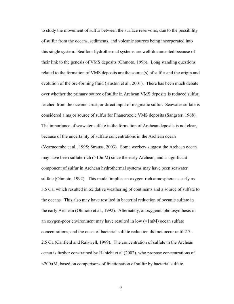
The sources of both metals and sulfur are linked to hydrothermal circulation

through oceanic crust (Franklin et al, 1981). Cold seawater seeps into the crust where

it is heated by shallow igneous bodies (Fig. 4) (Gibson et al., 1999). At low initial

temperatures (<150ºC), fixation of alkalis such as Na and K in the crust occurs, and

Mg from seawater is precipitated as smectite (Alt, 1999). Once fluid temperatures

increase, much of the dissolved seawater sulfate precipitates as anhydrite, and

remaining Mg reacts with water to form chlorite, causing the pH of the fluid to

decrease (Alt, 1999). Any remaining sulfate is inorganically reduced, either by

oxidation of reduced Fe in the host rock (Huston et al., 2001):

3224 48 OFeSHHFeOHSO Rock +=+= +− (1.5)

or by oxidation of pyrrhotite to pyrite (Shanks and Seyfried, 1987):

11

+−+ +++=++ 2222

24 444108 FeOHSHFeSSOHFeS (1.6).

As temperatures reach a maximum (>350ºC) at the reaction zone, metals and reduced

sulfur are leached from the rock (Fig. 4) (Alt, 1999). Possible direct contributions of

metal and sulfur from magmatic fluids have also been suggested (Yang and Scott;

1996). The fluid ascends rapidly to the surface where it mixes with seawater, and

precipitation of sulfide minerals occurs (Franklin et al., 1981), resulting in subsurface

mineralization or seafloor venting at black smokers (Alt, 1999).

Changes in environmental conditions over time, such as ocean sulfate

concentrations, global thermal regimes, and biological evolution, may have resulted

in formation processes for modern VMS deposits that differ from that of ancient

examples.

1.6 Accomplishments of this Thesis

The purpose of this thesis is to investigate the application of mass-

independent (∆33S) sulfur signatures as a tracer for sulfur mobility in Archean

hydrothermal systems. In particular, the following primary questions have been

addressed:

1. Can ∆33S values be used to trace different sources of sulfur through

ancient hydrothermal systems?

2. What are the sources of sulfur for Archean VMS deposits?

In attempting to answer these primary questions, other questions related to Archean

surface environment, such as the chemistry of the Archean oceans, processes

occurring at seafloor hydrothermal vent sites and the possibility of ∆33S values as an

exploration vector for ore deposits were investigated.

12

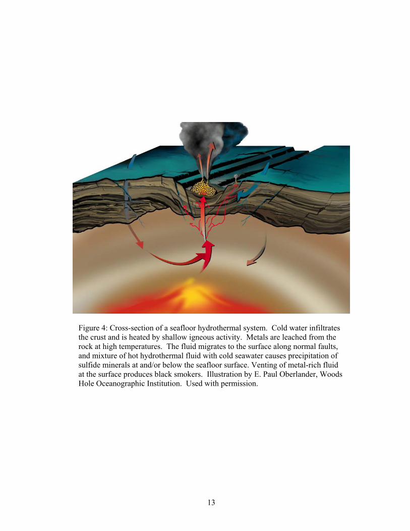
Figure 4: Cross-section of a seafloor hydrothermal system. Cold water infiltrates the crust and is heated by shallow igneous activity. Metals are leached from the rock at high temperatures. The fluid migrates to the surface along normal faults, and mixture of hot hydrothermal fluid with cold seawater causes precipitation of sulfide minerals at and/or below the seafloor surface. Venting of metal-rich fluid at the surface produces black smokers. Illustration by E. Paul Oberlander, Woods Hole Oceanographic Institution. Used with permission.

13

The use of ∆33S values to evaluate isotopic equilibrium in sulfide mineral

pairs is a new application of multiple sulfur isotopes that can be directly applied to

Archean ore deposit studies. This new tool for equilibrium evaluation will allow for

more reliable sulfur-isotope paleothermometry studies and differentiation of

ore forming events in single ore deposits.

Finally, this study will potentially lead to further applications of multiple

sulfur isotopes as a geochemical tool for investigations for Archean surface processes.

Sulfur isotope measurements of a full suite of samples from a well

characterized Archean VMS deposit were necessary for the scope of this study. The

2.7 Ga Kidd Creek deposit, in Ontario, Canada, is a world-class VMS deposit, and

has been the focus of many studies (most notably a major detailed study in the 1990s

by industry, government and university researchers, which resulted in the publication

of an Economic Geology Monograph) (Hannington and Barrie, 1999). This study has

led to a better understanding of the tectonic and surface environment in which the

deposit formed, as well as the physical and chemical processes involved in its

formation. The extensive geological and geochemical data available from this deposit

makes it an ideal location for this detailed investigation of the distribution of ∆33S

signatures in an ancient seafloor hydrothermal setting.

14

Chapter 2: Geological Background and Previous Work

2.1 The Kidd Creek Volcanogenic Massive Sulfide Deposit

The Kidd Creek VMS deposit is situated in the Abitibi granite-greenstone

belt, within the Superior craton, in eastern Ontario, Canada. The Abitibi subprovince

is thought to represent a series of granite-greenstone terrains, formed by accretion of

volcanic arcs and oceanic plateaus from ~2.8 to ~2.6 Ga (Langford and Morin, 1976;

Jackson and Cruden, 1995; Ludden and Hubert, 1986). The ore deposit is located in a

suite of bimodal (felsic, mafic and ultramafic) volcanics of the Kidd-Munro

assemblage, which formed between 2717 and 2711 Ma (Corfu, 1993; Bleeker, 1999).

The mine succession consists of basal komatiitic flows, followed by a lower massive

rhyolite unit and an upper fragmental rhyolite unit, which hosts the sulfide ore

(Barrie, 1999; Prior et al., 1999). Above the rhyolite is a quartz porphyry rhyolite,

followed by mafic volcanic rocks consisting of pillow lavas and breccias, with

interflow graphitic argillites (Hannington et al., 1999). The entire mine sequence is

intruded by gabbroic dykes and a large gabbroic sill overlies the quartz porphyry.

The lower boundary of the mine sequence is a fault or unconformity that separates the

volcanic succession from greywackes of the Porcupine Group that are younger than

2699 Ma (Bleeker and Parrish, 1996).

The mine stratigraphy at Kidd Creek has undergone multiple deformation

events, producing ore bodies that may be truncated, stretched, and over-thickened

(Bleeker, 1999). A series of folding events have produced a large scale interference

15

structure (Hannington et al., 1999). The deformation is systematic throughout the

mine stratigraphy, which has made it possible to reconstruct the original geometry,

and the depositional history of the ore deposit (Bleeker, 1999).

The volcanic succession at Kidd Creek was erupted during seafloor rifting,

likely in a back-arc basin (Bleeker et al., 1999) or mid-oceanic rift (Prior et al., 1999).

Hydrothermal circulation of seawater, driven by shallow igneous activity at the

spreading center, caused focused discharge of an evolved fluid along steeply dipping

normal faults, which bound a topographic low on the seafloor (Huston and Taylor,

1999). Precipitation of sulfide minerals occurred when the hot fluid mixed with cold

seawater (Pottorf and Barnes, 1983). At Kidd Creek, ore precipitation occurred

mostly below the seafloor, by infilling and replacement of rhyolite flows and

volcanoclastics in a seafloor graben or half-graben (Hannington et al., 1999a). Minor

focused venting of hydrothermal fluids at the seafloor resulted in surface

mineralization and the development of vent complexes (Hannington et al., 1999a).

Massive sulfide occurs as three distinct lenses within the rhyolite: the north,

central, and south orebody (Fig. 5) (Hannington et al., 1999a). The lenses are

composed primarily of massive pyrite and sphalerite, with minor pyrrhotite and

galena (Fig. 6A). Evidence of seafloor exposure and vent complexes takes the form

of sinters and sulfide debris flows near the top of the north orebody, and suggests that

parts of this lens were exposed at the surface (Hannington et al., 1999a). The lack of

such features in the central and south orebodies suggests that these lenses formed

entirely below the seafloor.

16

Figure 5: Cross-section (reconstructed) of Kidd Creek, showing the massive sulfide lenses (red), with underlying Cu-rich feeder zones (yellow) in a rhyolite host rock. The faulted is bounded to the north by a major structural discontinuity. (NOB = North Ore Body; COB = Central Ore Body; SOB = South Ore Body). Modified from Hannington et al. (1999)

17

The underside of each lens has a characteristic Cu-rich zone, composed

primarily of chalcopyrite, which formed by replacement of sphalerite during a late

stage injections of Cu-rich fluids (Fig. 6C) (Hannington et al., 1999). The sphalerite

reprecipitated at higher levels in the massive sulfide lenses. Beneath the south

orebody is a high-grade bornite zone, which represents an influx of a large amount of

an end-member, Cu-rich fluid, during the late stages of ore formation Fig. 6D)

(Hannington et al., 1999b). An extensive Cu-rich stockwork feeder zone underlies

the ore lenses, and reflects the upward-directed, down-temperature flow pathway of

the metal-rich hydrothermal fluid (Fig. 5) (Koopman et al., 1999). For the purposes

of this discussion, the ore lenses, bornite zone and Cu-rich stringer zones are

collectively referred to as massive sulfide.

Sulfides (mostly sphalerite and pyrite) also occur along the flanks of the

orebodies, as minor stringers and disseminations (Hannington et al., 1999a). These

zones of stratabound stringer and disseminated mineralization, hosted in brecciated

rhyolite, extend laterally from the massive sulfide lenses (Fig. 6B). The

concentration of sulfide minerals in these zones is significantly less than the

concentrations in the massive sulfides, and the ore minerals are referred to as wall-

rock sulfides.

Stratigraphically above the north and central orebodies, but in the footwall of

the south orebody, is a graphitic argillite that is rich in sulfide debris flows, as well as

pyrite nodules (Fig. 6F). These sulfides are thought to have a hydrothermal or

diagenetic origin (Hannington et al., 1999). This sedimentary unit likely formed

during a hiatus in volcanic activity on the seafloor. Debris flows, composed of pyrite

18

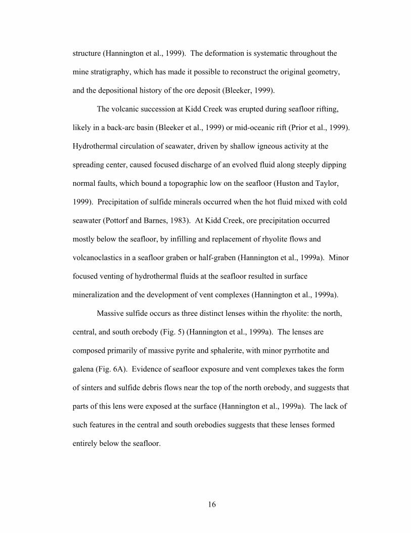
Figure 6: Representative ore textures from Kidd Creek. A. Fragmental massive pyrite and relict sphalerite clasts from top of massive sulfide lens. B. Pyrite and galena rich fragmental rhyolite, with a large sphalerite clast. C. Folded contact between massive sphalerite and chalcopyrite at base of north orebody. D. Massive bornite with relict chalcopyrite and pyrite porphyroblasts. E. Laminated quartz and sphalerite sinter above north orebody. F. Laminated graphitic argillite with graded sphalerite-rich turbidites. Photographs courtesy of Mark Hannington, University of Ottawa.

19

and sphalerite, occur within the argillite. These sulfide flows contain graded bedding,

and other sedimentary features, such as load casts and flame structures. These

turbiditic flows are thought to represent chimney collapse and mass-wasting events of

vent sulfides from the topographically high hydrothermal mound at the discharge site,

into the graben basin (Hannington et al, 1999a). Sulfides from these flows are

referred to as sulfide turbidites.

Direct precipitation of sulfide minerals onto the seafloor on the north orebody

resulted in sulfide-rich chemical sedimentary crusts (Fig 6E). These crusts are found

predominantly at the top of the north orebody, which was exposed at the seafloor.

Samples from these chemical crusts are referred to as sulfide-rich sinter.

2.2 Previous Sulfur-isotope Studies of Kidd Creek

The sulfur isotope ratios of Kidd Creek sulfides have been investigated in two

previous studies (Strauss, 1989; Hannington et al., 1999a). In both studies, sulfur

isotopes were measured from sulfides in the main orebodies, and hydrothermal

sulfides in the argillitic sediments above the orebodies.

The δ34S values from the main massive sulfide bodies clustered near 0‰,

which is typical for Archean massive sulfide deposits (Franklin et al., 1981). Strauss

(1989) interprets this isotopic signature to indicate a magmatic source for the sulfur in

the massive sulfides. The non-ore sulfides within the argillites have slightly more

positive δ34S values. Strauss (1989) interprets these values to result from inorganic

reduction of seawater sulfate. Bacterial sulfate reduction is not considered a

mechanism in the formation of these argillite-hosted sulfides, insofar as biogenic

20

sulfides precipitated by sulfate-reducing bacteria are not believed to appear before 2.4

to 2.2 Ga (Strauss, 1989).

Hannington et al. (1999a) observed little variation in δ34S values between the

three main ore lenses, and suggest a homogenous sulfur source for the orebodies. The

isotopic compositions of the massive sulfides are thought to reflect the primary

hydrothermal signature. The sulfides within the argillite are isotopically heavier than

the massive sulfides, and have a larger range in δ34S values. This is interpreted to

reflect variable sulfur sources within these units, which may have included inorganic

reduction of seawater sulfate.

21

Chapter 3: Methods

3.1 Sulfur Isotope Measurements

Sulfide mineral samples from the Kidd Creek VMS deposit were collected by

Mark Hannington as part of a comprehensive study of the ore deposit that resulted in

the publication of Economic Geology Monograph 10. Samples were collected from

the open pit, underground mining operations, diamond drill core, and surrounding

surface exposures. Regional hydrothermal sulfides from the Kidd-Munro assemblage

were also included. The samples were crushed and minerals separated at the

Geological Survey of Canada. Sulfur isotope measurements on sulfide mineral

separates were performed at the Stable Isotope Laboratory, University of Maryland.

Sulfur isotope analyses largely followed the methods of Rumble et al. (1993)

and Hu et al. (2003). Sulfides were converted to SF6 gas and other fluoride

compounds by heating the minerals under a ~40 Torr F2 atmosphere with a 25W CO2

infrared laser (λ = 10.6 µm). The resulting SF6 and condensable impurities were

condensed and separated from non-condensable gaseous fluoride compounds using an

N2 cryogenic trap (-196˚C). The liquid nitrogen trap was then evacuated of non-

condensable gases and warmed with an ethanol slush (-110˚C) to release SF6. The

SF6 was transferred to an injection loop and then passed through a gas chromatograph

to separate and remove remaining impurities. Purified SF6 was introduced to a

ThermoFinnigan MAT 253 dual-inlet gas-source mass spectrometer, which analyses

gaseous compounds by first ionizing the compounds to SF5+, then accelerating them

22

through a flight tube where their paths are deflected by a magnetic field. The amount

of deflection is a function of the charge-to-mass ratio of the compounds. The sulfur

isotope abundances for this project were measured by monitoring the 32SF5+, 33SF5

+,

34SF5+ ion beams at m/z = 127, 128, and 129, respectively. We did not carry out the

multiple purifications through the gas chromatograph that are required to remove

compounds producing isobaric interferences at m/z = 131 (such as C3F5) (Gao and

Thiemens, 1991; Rumble et al., 1993; Hu et al., 2003). Therefore, although the 36SF5+

ion beam was monitored and 36S measurements are included in the results, only 32S,

33S, and 34S measurements are used for purposes of our geologic interpretation and

discussion.

3.2 Interpretational Framework

Traditional three-isotope plots (δ33S vs. δ34S) are the most common way to

express multiple isotope ratios. These plots clearly illustrate the mass-dependent

fractionation relationship between the isotope ratios, and samples that do not strictly

follow this relationship (Fig. 1). However, for typical natural ranges in δ34S (and, by

association, δ33S) values, ∆33S values must be large to be clearly identified. In other

words, data points that have only small, but statistically significant (resolvable within

uncertainty) ∆33S values will plot close to the terrestrial fractionation line, and thus

may be wrongly interpreted as having a mass-dependent isotopic composition.

Samples with ∆33S values between -0.01 and 0.01‰ are considered mass-dependent.

Results of isotopic analyses of individual sulfide samples can also be plotted

on a ∆33S vs. δ34S diagram. The two axes can be scaled independently so that the

maximum range in ∆33S as well as δ34S values can be displayed. Samples with mass-

23

dependent sulfur will have a ∆33S value near 0 per mil. The ∆33S of samples with an

added component having negative ∆33S values, such as Archean sulfate, will reflect

this contribution and will plot below the x-axis. Samples that have incorporated

sulfur with positive ∆33S, such as Archean reduced sulfur in sediments, will plot

above the x-axis. Data arrays on this type of plot can also be interpreted for sample

sets that exhibit either small or large ranges in δ34S and ∆33S values.

Paleotemperatures were calculated from sulfide mineral pairs. The pairs

consisted of combinations of six different sulfide minerals, and eight independent

pairs were analyzed. Calibrations for isotope thermometers are from Ohmoto and

Rye (1979) and are shown in Table 1.

3.3 Analytical Uncertainties

Reproducibility of the entire measurement procedure was evaluated by repeat

analyses of an in-house pyrite working standard (see Appendix). Multiple

measurements of this standard (n=10) indicate that δ34S was measured with an

external reproducibility of ±0.22 ‰ (1σ), and δ33S with a long-term reproducibility of

±0.11 ‰ (1σ). Similar tests for ∆33S yield an external reproducibility of ±0.009 ‰

(1σ). Most of the variation in δ33S and δ34S is due to minor mass-dependent

fractionation inherent in the measurement procedure, as indicated by the difference

between the experimentally determined reproducibility for ∆33S (0.009 ‰) and the

uncertainty predicted by propagation of uncorrelated experimental uncertainties for

δ33S and δ34S through the definition of ∆33S (0.158 ‰) (see Apendix).

24

Table 1: (from Ohmoto and Rye, 1979)

⎟⎟⎠

⎞⎜⎜⎝

⎛++

×=

10001000ln1000

10

34

34

6

Y

X

SS

AT

δδ

Calibrations for Sulfur Isotope Thermometers Mineral X Mineral Y Value “A”

Pyrite Galena 1.03 Pyrite Sphalerite or Pyrrhotite 0.3

Chalcopyrite Bornite 0.2 Sphalerite or Pyrrhotite Chalcopyrite 0.15

25

Calculated ∆33S values vary depending on the value of λ used in equation 1.3.

Theorietical calculations indicate that equilibrium processes produce λ values that

range from 0.513 to 0.518 (Hulston and Thode, 1965). This variation results in a

∆33S value that can vary by 0.003 ‰, for every per mil shift in a δ34S value. The

range in measured δ34S values at Kidd Creek results in a possible variation in ∆33S

values of 0.01 ‰, which is less than the 2σ experimental reproducibility of the

measured ∆33S values (0.018 ‰).

26

Chapter 4: Results

4.1 Kidd Creek Sulfides

Sulfur isotope ratios (δ33S, δ34S, and ∆33S) of fifty-five sulfide samples from

the Kidd Creek ore deposit are presented in Table 2. The results are illustrated on a

traditional three-isotope plot (Fig. 7) and on a ∆33S vs. δ34S plot (Fig. 8). Because of

the expanded scale, the ∆33S- δ34S diagram in Figure 8 illustrates more clearly the

degree of non-mass-dependence in the samples. The data include sulfides from the

main ore deposit as well as sulfides from the surrounding country rock. The δ34S

values range from -4.26 to 5.46 ‰, with a mean value of 0.72 (± 1.82) ‰ (1σ).

Mass-independent signatures (∆33S) were calculated for all samples, using equation

(1.3). Values of ∆33S range from -1.50 to 1.12 ‰.

The analyzed samples are divided into four groups, based on textural features

of the sulfides and the host rock. Together, these features ultimately correlate to the

location and environment of precipitation within the ore deposit. The most common

ore type is massive sulfide, which occupies the three main ore lenses near the top of

the deposit succession, and their accompanying Cu-rich feeder zones. Also included

is the high-grade bornite zone beneath the south ore body. The massive sulfides

represent precipitation of ore by epigenetic replacement of rhyolite below the seafloor

during mixing of the hot hydrothermal fluids with cold seawater. Sulfide minerals

analyzed in this study include pyrite, sphalerite, chalcopyrite, pyrrhotite, galena and

27

Table 2: Isotopic analyses of sulfides from Kidd Creek Sample Mineral δ33SV-CDT

(‰) δ34SV-CDT

(‰) δ36SV-CDT

(‰) ∆33S (‰)

∆36S (‰)

Massive Sulfides KCP53_2 Gn -1.64 -3.01 -5.03 -0.09 0.68 KC5 Bn -0.84 -1.57 -1.93 -0.03 1.05 KC350_A1 Bn -0.81 -1.51 -2.33 -0.03 0.54 KC349 Bn -0.41 -0.73 -0.71 -0.04 0.67 KC350_A2 Cp -0.40 -0.71 -0.74 -0.04 0.61 KC5 Cp -0.39 -0.71 -0.64 -0.03 0.70 KC8 Py -0.28 -0.53 9.46 -0.01 10.47 KC17B Sp -0.31 -0.43 -0.07 -0.09 0.75 KC93 Sp -0.19 -0.31 1.62 -0.03 2.21 MH184_1 Cp -0.18 -0.31 0.43 -0.02 1.02 KC451_1 Po-Sp -0.20 -0.28 0.05 -0.05 0.58 KC48 Py -0.19 -0.27 0.22 -0.05 0.73 KC29B Sp -0.18 -0.26 0.46 -0.05 0.95 KC29B Sp 0.02 0.12 0.96 -0.04 0.74 KC86 Sp -0.13 -0.10 0.55 -0.08 0.74 KC36 Cp -0.06 -0.06 0.62 -0.03 0.73 KC36 Cp 0.42 0.83 2.12 -0.00 0.55 KC451_2 Sp -0.06 -0.04 0.63 -0.04 0.71 KCP36B Cp -0.03 -0.01 0.71 -0.03 0.74 KC12 Cp 0.01 0.08 0.54 -0.04 0.39 KC12 Cp -0.03 -0.03 0.46 -0.02 0.51 KC93 Po 0.03 0.16 0.97 -0.05 0.66 KC6B Cp 0.05 0.17 0.95 -0.04 0.62 KC96 Cp 0.06 0.18 0.76 -0.03 0.42 KC83A Py 0.12 0.24 1.11 -0.01 0.67 KC43 Cp 0.09 0.28 8.32 -0.05 7.80 KC111 Sp 0.12 0.34 1.03 -0.05 0.39 KC43 Po 0.14 0.37 1.16 -0.05 0.45 KC9A Cp 0.20 0.37 1.52 0.01 0.81 KC44 Cp 0.25 0.47 1.71 0.01 0.83 KC83A Sp 0.20 0.51 1.52 -0.07 0.55 KC121 Py 0.24 0.55 1.71 -0.04 0.67 KC121 Py 0.21 0.50 1.66 -0.04 0.72 KC65A Cp 0.35 0.73 1.48 -0.02 0.09 KC29B Po 0.37 0.73 1.90 0.00 0.50 KC15 Py 0.27 0.76 2.42 -0.12 0.97 KC110 Sp 0.58 1.15 3.06 -0.01 0.86 KC53-1 Py 0.63 1.34 2.95 -0.06 0.40 KC52B Py 0.73 1.79 3.71 -0.19 0.30 KC95 Cp 1.15 2.22 4.69 0.00 0.47

(Continued next page)

28

Table 2: Isotopic analyses of sulfides from Kidd Creek (cont.)

Sample Mineral δ33SV-CDT δ34SV-CDT δ36SV-CDT ∆33S ∆36S

Wallrock Sulfides KC307 Py 0.32 0.69 1.54 -0.04 0.22 KC475 Py 1.36 2.78 6.14 -0.07 0.85 KC375 Py 2.34 4.84 10.02 -0.15 0.80 Sulfide-rich Sinter KCP47 Py -0.16 -0.15 0.19 -0.08 0.48 KCP45A Py 0.52 0.18 0.65 0.43 0.31 KC130 Py 1.73 1.72 3.17 0.84 -0.09 Sulfide Turbidites KCC13-2 Py -1.49 -4.26 -8.99 0.71 -0.92 KCR34-1 Py -2.04 -3.18 -5.87 -0.40 0.16 KCC13-1 Py -0.38 1.14 3.58 -0.96 1.41 KC129 Py 0.59 1.33 3.39 -0.09 0.85 KCC14-3 Py 1.81 1.47 2.47 1.05 -0.32 KCC14-1 Py 0.75 1.57 3.63 -0.06 0.65 KCR45B Py 0.41 1.66 3.86 -0.44 0.71 KCR34-2 Py 0.56 1.91 4.62 -0.43 0.98 KCP5 Py 0.90 1.99 4.55 -0.13 0.76 KCP5 Py 0.95 2.08 4.49 -0.12 0.55 KCC14-2 Py 1.10 2.01 4.17 0.06 0.35 KCR44 Py 2.75 3.18 4.64 1.12 -1.40 KCR44 Py 2.79 3.27 4.79 1.11 -1.43 KCCARN-4 Py 1.23 4.92 11.03 -1.31 1.66 KC4509 Py 1.31 5.46 12.15 -1.50 1.75 KC4509 Py 1.34 5.20 11.80 -1.34 1.90 Note: Samples with repeat measurements are plotted in Figures 7 and 8 as average

values.

Table 3: Mineral Abbreviations (from Kretz, 1983):

Mineral AbbreviationPyrite Py

Pyrrhotite Po Sphalerite Sp

Galena Gn Chalcopyrite Ccp

Bornite Bn

29

Figure 7: Traditional three-isotope plot of sulfides from Kidd Creek (similar to Figure1). Samples with mass-independent signatures plot above or below the TFL.

30

Figure 8: This plot shows in more detail the ∆33S values of the sulfides at Kidd Creek. The massive sulfides and wall-rock sulfides have a narrow range of ∆33S values, whereas the sulfide-rich sinter and sulfide turbidite show large variations in ∆33S values.

31

bornite. The massive sulfides have a δ34S range of -3.01 to 2.22 ‰ and a ∆33S range

of -0.19 to 0.01 ‰ (n=36), showing a spread in δ34S values with little variation in

∆33S values. Of these samples, only three have positive ∆33S values. The majority of

the samples have negative ∆33S values that do not overlap the mass-dependent line (x-

axis in Fig. 8).

Wall-rock sulfides consist of pyrite and sphalerite staining within the

fragmental rhyolite that hosts the main lenses (Koopman et al., 1999). Staining

consists of microscopic disseminations and diffuse patches in silicified cherty

breccias and occurs in the hanging wall of the deposit and laterally from the main

lenses and precipitated from diffuse flow of hydrothermal fluids (Koopman et al.,

1999). The δ34S values of the three wall-rock sulfides analyzed range from 0.69 to

4.84 ‰, and the ∆33S are all negative, with values that range from -0.15 to -0.04 ‰.

This range is similar to the ∆33S range in the massive sulfides.

The three samples grouped as sulfide-rich sinter represent sulfides that formed

as direct precipitates on the seafloor at the site of hydrothermal discharge. These

samples occur as pyrite replacing sphalerite in laminated argillaceous units that were

deposited on the flanks of the seafloor hydrothermal mound. Sulfide sinter is not

common at Kidd Creek, as the majority of sulfides precipitated below the seafloor.

The δ34S values of the sulfide sinter range from -0.15 to 1.72 ‰ (two of the three

samples have δ34S values that, within uncertainty, are 0 ‰) and the ∆33S values range

from -0.08 to 0.84 ‰. The only sulfide sinter sample with a negative ∆33S value plots

in the same field as the massive sulfides. The other two sulfide sinter samples have

significantly higher ∆33S values.

32

The final group of sulfides, sulfide turbidites, is interpreted to represent

remains of collapsed sulfide vent chimneys. Collapses of the fragile chimneys result

in sulfide-rich debris, which flows off the flanks of the hydrothermal mounds, and

into graphitic and argillaceous sediments (Hannington, pers. comm.). Sulfides occur

as laminated pyrite horizons with nodular pyrite and sphalerite replacement features.

This group contains the largest variations in isotope ratios, both for δ34S values and

∆33S values. For the 13 samples analyzed, δ34S values range from -4.27 to 5.46 ‰

and ∆33S values range from -1.50 to 1.12 ‰. These values represent the extreme

positive and negative δ34S and ∆33S values for all the hydrothermal sulfides analyzed

at Kidd Creek.

4.2 Sulfide Mineral Pairs

Measured δ33S, δ34S, and ∆33S values for eight sulfide mineral pairs are

reported in Table 4, which also shows calculated paleotemperatures. All eight pairs

are from massive sulfides of the main ore lenses or the bornite zone. For this study,

minerals from the same hand specimen and, in most cases, from the same part of a

hand specimen (i.e., a discrete mineral association or zone) are considered pairs. Co-

precipitation is not a requirement for two minerals to be considered pairs.

Five mineral pairs from the north orebody were analyzed; three sphalerite-

pyrrhotite pairs (#s 4, 5 and 6), a sphalerite-pyrite pair (#7) and a galena-pyrite pair

(#3) (Table 4). The two bornite-chalcopyrite mineral pairs (#s 1 and 2) are from the

high-grade bornite zone beneath the south orebody and the chalcopyrite-pyrrhotite

pair (#8) is from the Cu-rich stringer zone, beneath the orebodies.

33

TABLE 4. Summary of Sulfur Isotopic Data of Mineral Pairs from Kidd Creek

Pair Sample Mineralogy δ33SV-CDT (‰)

δ34SV-CDT (‰) ∆33S1

Temperature2

(Celsius) σT

3

(Celsius)

KC 5 Bn -0.84 -1.57 -0.029 1 KC 5 Ccp -0.39 -0.71 -0.030 209 234

KC 350-A1 Bn -0.81 -1.51 -0.026 2 KC 350-A2 Ccp -0.40 -0.71 -0.039 227 245

KCP 53-2 Gn -1.64 -3.01 -0.088 3 KCP 53-1 Py 0.63 1.34 -0.056 213 35

KC 93 Sp -0.19 -0.31 -0.028 4 KC 93 Po 0.03 0.16 -0.050 N/A4 N/A

KC 451-1 Po -0.20 -0.28 -0.054 5 KC 451-2 Sp -0.06 -0.04 -0.041 N/A4 N/A

KC 29B Sp -0.18 -0.26 -0.050 6 KC 29B Po 0.37 0.73 -0.004 N/A4 N/A

KC 83A Py 0.12 0.24 -0.005 7 KC 83A Sp 0.20 0.51 -0.067 Reversed5 N/A

KC 43 Ccp 0.09 0.28 -0.049 8 KC 43 Po 0.14 0.37 -0.048 1018 2300

1Values of ∆33S are calculated using the relationship 1000111000

SSSRFL34

3333 ×⎥⎥⎦

⎤

⎢⎢⎣

⎡−⎟⎟

⎠

⎞⎜⎜⎝

⎛+−=∆

λδδ

2Temperatures are calculated using values and equation from Table 10-1 of Ohmoto and Rye (1979) 3Uncertainties in temperature are calculated using method of Farquhar et al. (1993):

( ) ( )⎥⎥⎥⎥⎥

⎦

⎤

⎢⎢⎢⎢⎢

⎣

⎡⎟⎟⎠

⎞⎜⎜⎝

⎛++

++

++

×

⎥⎥⎥⎥⎥

⎦

⎤

⎢⎢⎢⎢⎢

⎣

⎡

⎟⎟⎠

⎞⎜⎜⎝

⎛++

×=

−

−−

2

2

34

342

234

2

234

2

3

34

34

10001000ln

1000100010001000ln4

1000 3434

BA

B

AA

B

S

A

S

B

A

BAT A

SS

SSSS

A BA

BAδδσ

δ

σ

δ

σ

δδ

σ δδ

4Equilibrium fractionation between sphalerite and pyrrhotite is negligible, therefore temperatures cannot be calculated from these minerals 5Pyrite must be isotopically heavier than sphalerite for a temperature to be calculated using these minerals

34

Chapter 5: Discussion

5.1 Sources of Sulfur at Kidd Creek

Sulfide minerals at Kidd Creek have a range of ∆33S values indicating

multiple sources of sulfur within the overall deposit. Minerals with positive ∆33S

values contain sulfur with a component of S8 in the water column that has been

reduced. Samples with negative ∆33S values have a component of sulfur from

seawater sulfate.

The range in ∆33S values of the massive sulfides is small, and suggests a

common source of sulfur for the three ore lenses, the bornite zone and the Cu-rich

feeder zone, beneath the orebodies. The range in δ34S values within the massive

sulfides can be attributed to equilibrium fractionation between different sulfide

minerals (see section 5.2).

The wall-rock sulfides are interpreted to be of hydrothermal origin and have a

∆33S signature that is within the range of ∆33S values of the massive sulfides,

suggesting that the disseminated and nodular sulfides in the host rhyolite precipitated

from the same fluid that formed the massive sulfides with their associated stringer

zones.

Of the three sulfide samples extracted from the sulfide-rich sinter, two have

∆33S values suggesting a significant component of sulfide that is reduced directly

from the water column, likely by a chemical process. Anaerobic reduction by non-

35

photosynthesizing bacteria is not thought to be active at this time (Canfield and

Raiswell, 1999). The third sample has an isotopic composition that plots within the

range of the massive sulfides, indicating the possibility of a common source. The

range in ∆33S values between the three sinter samples indicates that the source of

sulfur for sulfides precipitating from the hydrothermal fluid on the seafloor at the site

of discharge is itself heterogeneous, with differing proportions of sulfur from

sedimentary sources, seawater sulfate and volcanic sulfur.

The range in ∆33S values for the sulfide turbidites shows the largest

heterogeneity from a single genetic environment within the ore deposit. The ∆33S

values indicate significant contributions from volcanic sources, seawater sulfate and

native sulfur.

The sulfides, categorized by environment of precipitation or deposition, can

be further grouped according to their ∆33S values. The massive sulfides and wall-

rock sulfides all precipitated below the seafloor, and have a small range in ∆33S. The

sulfide-rich sinter and sulfide turbidites can be grouped together as surface

hydrothermal sulfides, and are distinguished by the large range in ∆33S values. The

difference in magnitudes and range of ∆33S values between the surface and subsurface

sulfides indicates a distinct difference in the sulfur chemistry of ore formation.

The subsurface ore has a slight, but consistently negative ∆33S signature,

indicating a minor contribution of seawater sulfate to an ore-forming fluid dominated

by volcanic sulfur. The volcanic sulfur was either leached from the oceanic crust or

sourced directly from the magmatic intrusion that is driving the hydrothermal

circulation. The ∆33S signatures of primary magmatic sulfur and leached rock sulfur

36

are likely indistinguishable, as neither reservoir contains significant amounts of

photochemically-derived sulfur. The ∆33S tool can therefore not be used to determine

the relative contributions of these two sulfur sources, and independent methods, such

as Se/S ratios must be applied (Huston et al., 1995).

The small range in ∆33S values indicates a well-mixed source, suggesting that

the sulfur was transported to the site of precipitation by the hydrothermal fluid, and

there was no mixing with coeval surface sources. This suggests, therefore, that the

seawater sulfate was incorporated into the hydrothermal fluid by a uniform process

such as during recharge at the seafloor and transported through the hydrothermal

system. The dissolved sulfate was abiotically reduced and mixed with reduced rock

sulfur, forming a homogenized sulfur source in the hydrothermal fluid in the upflow

zone, and ultimately at the site of subsurface sulfide precipitation.

The large magnitude (positive and negative), and range of ∆33S values for the

surface sulfides indicates multiple, non-homogenized sulfur sources, which may

include the hydrothermal sulfur that formed the subsurface deposits. Larger ∆33S

values indicate lower contributions of hydrothermal-derived sulfur and higher

contributions of local dissolved sulfate (negative ∆33S values) or locally derived

native sulfur (positive ∆33S values). Contributions of non-hydrothermal sulfur

directly form the water column would result in the incorporation of sulfur with ∆33S

compositions comparable to the most extreme positive and negative ∆33S values

recorded at Kidd Creek.

The sulfide turbidite samples, which represent collapsed vent chimneys, and

have highly negative ∆33S values, contain a large component of sulfur that was likely

37

directly reduced from sulfate in the water column. These turbidite horizons may also

incorporate minor amounts of non-hydrothermal sulfide from the sediment or directly

from the water column. These sulfides would likely have ∆33S compositions

comparable to the most extreme positive ∆33S values recorded at Kidd Creek.

Possible reductants include reduced iron from the hydrothermal fluid and organic

carbon in the sediment. The δ34S values of these samples range from 1.14 to 5.46 ‰,

and are isotopically heavier than the massive sulfides, which is consistent with a

reduced seawater sulfate source, relative to a volcanic-dominated source.

The positive ∆33S values, for sulfide turbidites and sulfide-rich sinter, are

interpreted to indicate that native sulfur (S8) was reduced directly from the water

column and incorporated into these surface hydrothermal sulfides, similar to the

sulfide-rich sinter. Figure 9 illustrates the different sulfur reservoirs, with their

associated ∆33S values, that are relevant to Archean hydrothermal circulation.

The incorporation of sulfur from the surface environment at the discharge site

suggests that the hydrothermal fluid was depleted in reduced sulfur, but not dissolved

metals. The bulk of the reduced sulfur in the hydrothermal fluid precipitated in the

subsurface. Excess dissolved metals that vented at the surface scavenged sulfur by

chemical reduction of dissolved sulfate and native sulfur in the water column.

Elevated ∆33S values in surface hydrothermal sulfides in Archean terrains may be an

indication of the proximity of significant massive sulfide that formed below the

seafloor. These values may serve as an exploration vector when exploring for VMS

deposits.

38

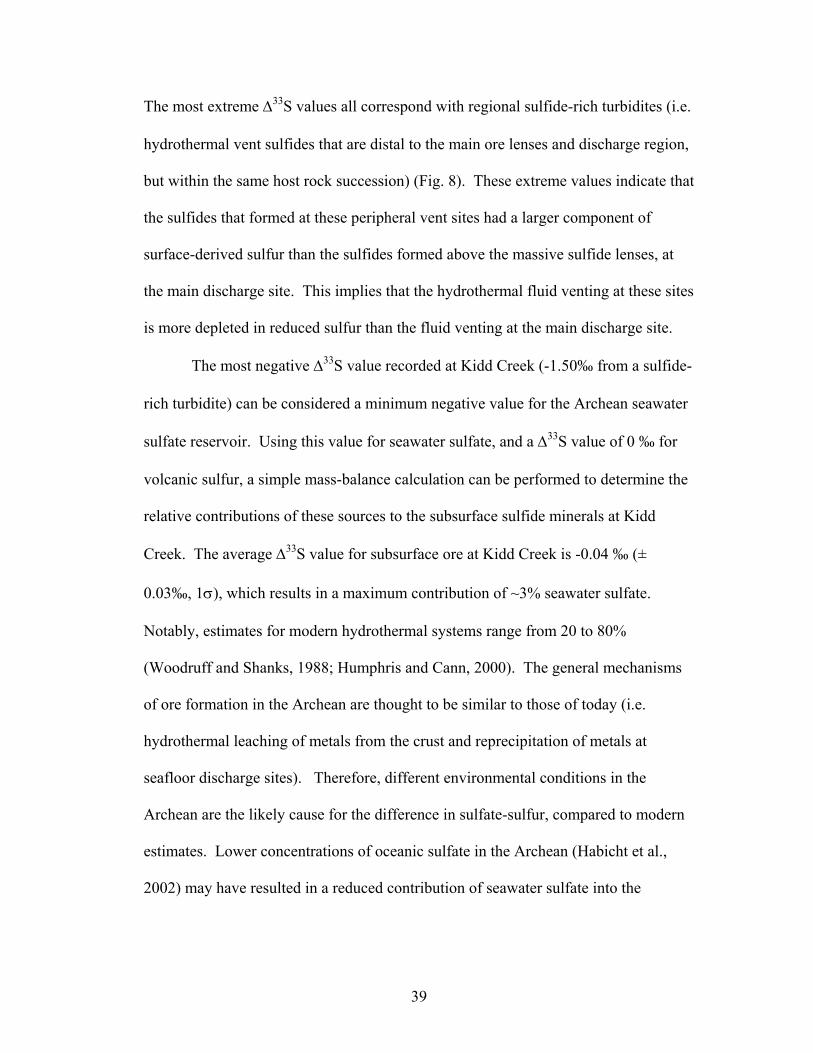
The most extreme ∆33S values all correspond with regional sulfide-rich turbidites (i.e.

hydrothermal vent sulfides that are distal to the main ore lenses and discharge region,

but within the same host rock succession) (Fig. 8). These extreme values indicate that

the sulfides that formed at these peripheral vent sites had a larger component of

surface-derived sulfur than the sulfides formed above the massive sulfide lenses, at

the main discharge site. This implies that the hydrothermal fluid venting at these sites

is more depleted in reduced sulfur than the fluid venting at the main discharge site.

The most negative ∆33S value recorded at Kidd Creek (-1.50‰ from a sulfide-

rich turbidite) can be considered a minimum negative value for the Archean seawater

sulfate reservoir. Using this value for seawater sulfate, and a ∆33S value of 0 ‰ for

volcanic sulfur, a simple mass-balance calculation can be performed to determine the

relative contributions of these sources to the subsurface sulfide minerals at Kidd

Creek. The average ∆33S value for subsurface ore at Kidd Creek is -0.04 ‰ (±

0.03‰, 1σ), which results in a maximum contribution of ~3% seawater sulfate.

Notably, estimates for modern hydrothermal systems range from 20 to 80%

(Woodruff and Shanks, 1988; Humphris and Cann, 2000). The general mechanisms

of ore formation in the Archean are thought to be similar to those of today (i.e.

hydrothermal leaching of metals from the crust and reprecipitation of metals at

seafloor discharge sites). Therefore, different environmental conditions in the

Archean are the likely cause for the difference in sulfate-sulfur, compared to modern

estimates. Lower concentrations of oceanic sulfate in the Archean (Habicht et al.,

2002) may have resulted in a reduced contribution of seawater sulfate into the

39

Figure 9: Conceptual diagram of surface sulfur reservoirs associated with seafloor hydrothermal circulation. Dissolved sulfate imparts a negative ∆33S signature on the hydrothermal fluid. This signature is diluted towards 0‰ by addition of juvenile sulfur, and recorded in subsurface massive sulfides. A proportion of surface sulfur in surface ore sulfides is scavenged from coeval seawater sulfate and reduced sedimentary sulfide.

40

hydrothermal system, which led to a higher relative contribution of juvenile sulfur in

the hydrothermal fluid at the discharge site. Higher heat flow in the Archean likely

resulted in more vigorous hydrothermal circulation through the crust. It is unclear if

increased circulation would affect the relative contributions of seawater sulfate and

juvenile sulfur. Higher heat may have increased the ability of fluid to leach sulfur

from the volcanic rock. However, the increased circulation would have also resulted

in an increase drawdown of dissolved sulfate, which could counteract the increase in

leached sulfur.

5.2 Isotopic Disequilibrium in Sulfide Mineral Pairs

The uses of ∆33S values have been largely restricted to tracing the movement

of sulfur between different Archean reservoirs. However, mass-independent

fractionation of sulfur isotopes in the Archean provides a tool that, in certain

geological environments, can be used to provide insights into the state of isotopic

equilibrium between mineral pairs.

Isotopic equilibrium in mineral pairs is essential for isotope-thermometry

calculations (Ohmoto and Rye, 1979). Suitability of mineral pairs for these

calculations is often evaluated by the consistency of calculated temperatures with

inferred geological conditions. If a temperature determined from a mineral pair is

within an estimated temperature range, that temperature is assumed to be accurate,

and the minerals in the pair are assumed to be in isotopic equilibrium, which may not

necessarily be a correct assumption. This reasoning is circular and other tests are

needed. A simple graphical test can be used to determine what mineral pairs are

consistent with equilibrium in a sample set with mass-independent fractionation, such

41

as the Kidd Creek sample set. The use of ∆33S values provides an independent tool

that can be used to identify pairs that are not in equilibrium, even though their

calculated temperatures appear to be reasonable.

Equilibrium in a multiple-isotope system with at least one source that is not on

the terrestrial fractionation line leads to the development of a secondary fractionation

array that is parallel to the reference mass-fractionation line (Fig. 10) (Matsuhisa et

al., 1978). In the sulfur multiple-isotope system, this secondary array would define a

constant value of ∆33S. Therefore, for two minerals to be in isotopic equilibrium they

must have similar ∆33S values. Although the same ∆33S value is a necessary

condition for isotopic equilibrium, it is not sufficient, and common ∆33S values could

instead indicate a shared sulfur source. However, dissimilar ∆33S values clearly

indicate isotopic disequilibrium between minerals.

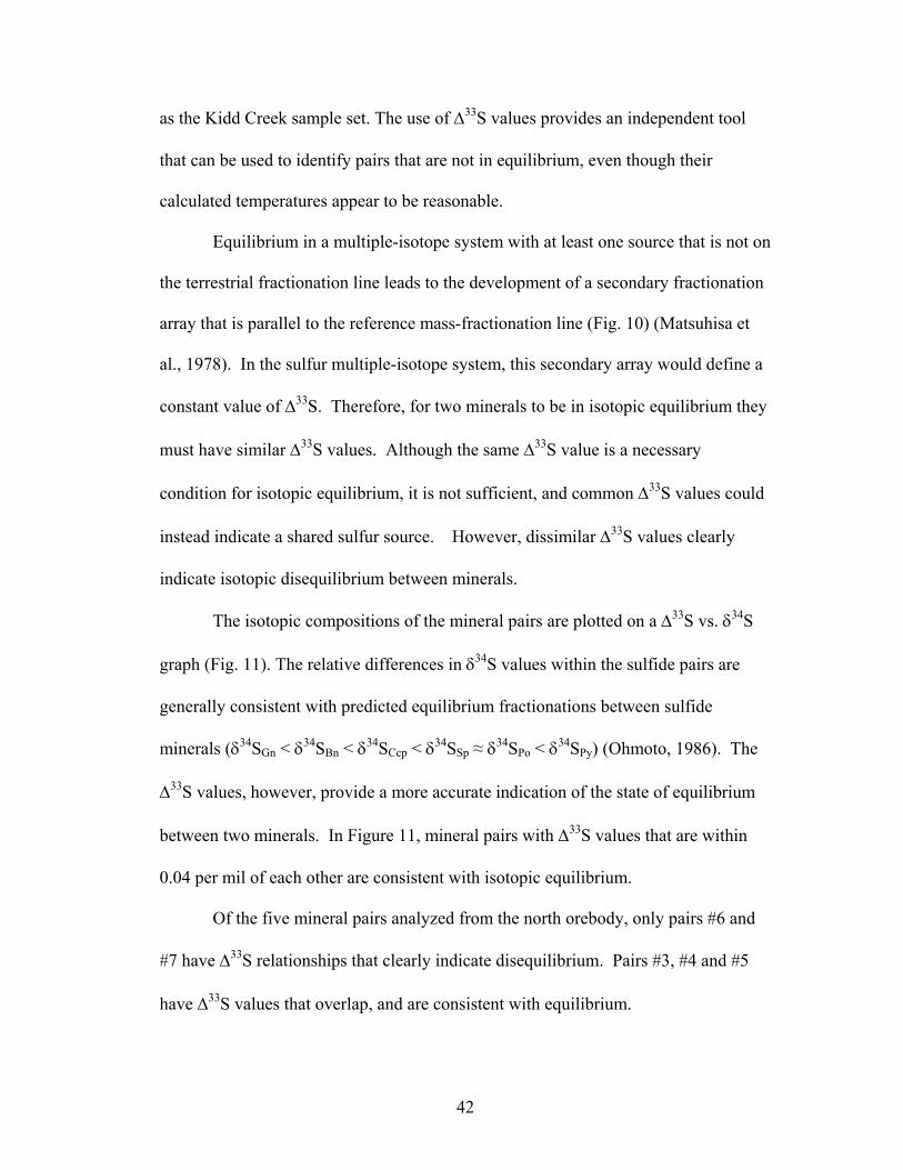
The isotopic compositions of the mineral pairs are plotted on a ∆33S vs. δ34S

graph (Fig. 11). The relative differences in δ34S values within the sulfide pairs are

generally consistent with predicted equilibrium fractionations between sulfide

minerals (δ34SGn < δ34SBn < δ34SCcp < δ34SSp ≈ δ34SPo < δ34SPy) (Ohmoto, 1986). The

∆33S values, however, provide a more accurate indication of the state of equilibrium

between two minerals. In Figure 11, mineral pairs with ∆33S values that are within

0.04 per mil of each other are consistent with isotopic equilibrium.

Of the five mineral pairs analyzed from the north orebody, only pairs #6 and

#7 have ∆33S relationships that clearly indicate disequilibrium. Pairs #3, #4 and #5

have ∆33S values that overlap, and are consistent with equilibrium.

42

Figure 10: Three isotope plots of system with bulk composition M and minerals A and B. 1: The isotopic composition of minerals A and B precipitating in equilibrium from a fluid with a composition M. Minerals A and B will fall on a common fractionation line with a slope parallel to the terrestrial fractionation line, resulting in similar ∆33S values. 2: The isotopic composition of minerals A and B (with different initial ∆33S values) will shift towards a secondary fractionation line during as they equilibrate.

43

Equilibrium fractionation between sphalerite and pyrrhotite is negligible, and

pyrrhotite-sphalerite mineral pairs in equilibrium should have similar δ34S values.

Pairs #4 and #5 have δ34S values that are within analytical uncertainty of each other

whereas pair #6 does not. These results are consistent with the equilibrium

relationships defined by ∆33S values. For pyrrhotite-sphalerite pairs, and other

mineral pairs with negligible equilibrium fractionation factors (such as millerite-

sphalerite; Ohomoto and Rye, 1979), ∆33S values provide the only isotopic evidence

for the state of equilibrium between the two minerals.

The disequilibrium relationship indicated by ∆33S values for the sphalerite-

pyrite pair (#7) is consistent with the δ34S relationship between the two minerals. The

pyrite in pair #7 is isotopically lighter than the sphalerite (Fig. 11). Under

equilibrium conditions, pyrite should have a more positive δ34S value than sphalerite

(Ohmoto and Rye, 1986). A paleotemperature can therefore not be calculated using

this pair.

Galena and pyrite have the largest fractionation under equilibrium conditions,

relative to the other major sulfides analyzed, making this mineral pair ideal for

paleothermometric calculations. The ∆33S values for this pair indicate consistency

with equilibrium. The δ34S values are also consistent with equilibrium fractionation,

and yield a calculated temperature of 213 degrees Celsius (± 35°C). This value is

consistent with temperatures predicted by Hannington et al. (1999a) for sulfide

precipitation in the massive sulfide lens, based on temperature-solubility models.

The ∆33S relationships for the two bornite-chalcopyrite mineral pairs (#s 1 and #2)

from the high-grade bornite zone are consistent with equilibrium. The bornite is

44

Figure 11: Sulfur multiple-isotope measurements for mineral pairs from Kidd Creek. Pairs are numbered and connected by broken tie-lines. Pairs in isotopic disequilibrium (colored in red) have tie lines that are not in experimental reproducibility of being parallel to the x-axis. Tie-lines that are parallel to the x-axis indicate consistency with isotopic equilibrium (colored in green). Pairs #6 and #7 are in isotopic disequilibrium. The other six pairs have ∆33S values that are consistent with equilibrium. Error bars indicate 2σ uncertainties.

45

thought to have formed by replacement of chalcopyrite. The similar ∆33S values

suggest that both minerals have the same sulfur source and replacement of

chalcopyrite by bornite involved addition of copper, but not sulfur. The difference in

δ34S values for the separate minerals in each pair yield paleotemperatures of 209

degrees Celsius (± 234˚C) for pair #1 and 227 degrees Celsius (± 245˚C) for pair #2.

These temperatures are consistent with temperatures calculated using independent

methods (Hannington et al, 1999a), which is further support of an equilibrium

relationship between these minerals. The large errors in calculated temperatures are

due to the small equilibrium fractionation between bornite and chalcopyrite.

The isotopic compositions of the chalcopyrite-pyrrhotite pair (#8), from the

copper stringer zone below the central orebody, plot within error of each other. The

∆33S values are consistent with isotopic equilibrium. Equilibrium isotopic

thermometry calculations are equivocal for this pair, and cannot bear on the

inferences based on ∆33S values. We note that similar ∆33S values are not sufficient

indicators for isotopic equilibrium as similar ∆33S values in mineral pairs can also be

caused by the minerals having the same sulfur source. It is not clear whether the

results from pair #8 reflect this situation, or whether they reflect the relative

imprecision of our δ34S measurements.

46

Chapter 6: Conclusions

The focused study of multiple sulfur isotope compositions of sulfides at the

Kidd Creek VMS deposit has demonstrated the use of atmospheric mass-independent

sulfur signatures as a tracer of the movement of sulfur, from different surface

reservoirs, through a seafloor hydrothermal system. Sulfur from seawater sulfate will

have a negative ∆33S value, sulfur from sedimentary sulfide will have a positive ∆33S

value, and juvenile sulfur has a ∆33S value of 0 ‰.

The sulfide ores at Kidd Creek can be grouped based on ∆33S values into two

environments of precipitation: subsurface ore, consisting of massive sulfide lenses, a

Cu-rich stringer zone and disseminated wall-rock sulfides, and surface sulfides, which

consist of sulfide-rich sinter and turbidites. The ∆33S values of the subsurface ore

show little variability, indicating a homogenous sulfur source. The ∆33S values are

slightly negative, indicating a minor component of sulfur from seawater sulfate in the

hydrothermal fluid. This sulfate was transported through the hydrothermal system

and was reduced by reactions with the wall rock. The majority of the reduced sulfur

in the hydrothermal fluid was leached from sulfides in the volcanic rocks. A

component of sulfur from magmatic fluids may be incorporated into the hydrothermal

fluid.

The surface sulfides have a wide range of positive and negative ∆33S values,

indicating multiple sources of sulfur, which is in contrast to the single, homogenized

source for the subsurface sulfur. Large negative ∆33S values indicate the reduction of

47

sulfur directly from seawater sulfate. Large positive values indicate remobilization

and incorporation of sedimentary sulfur during precipitation of hydrothermal sulfides.

A vent fluid that is depleted in reduced sulfur, but not dissolved metals, resulted in

the stripping of sulfur from the surface environment to precipitate metal sulfides. A

large surface sulfur signature may indicate the presence of significant subsurface

sulfide mineralization, and could be used as a potential exploration tool for VMS

deposits.

Using the most negative ∆33S value as an estimate for the mass-independent

signature of the Archean ocean sulfate reservoir, a mass-balance of a two component

system (volcanic sulfur and seawater sulfate) for the subsurface sulfides results in a

~3% contribution of seawater sulfate to the otherwise volcanic sulfur-dominated

hydrothermal fluid. This value is much lower than estimates of sulfate contributions

for modern hydrothermal systems, and may be a result of lower oceanic sulfate

concentrations in the Archean.

Sulfur multiple-isotope measurements also provide a natural reference frame

to evaluate isotopic disequilibrium between sulfide mineral pairs. When minerals are

in equilibrium, ∆33S values are similar; minerals in isotopic disequilibrium may have

different ∆33S values. This isotopic test for disequilibrium provides a criterion for the

suitability of mineral pairs for paleothermometry calculations that is independent of

conventional methods for evaluating disequilibrium. A unique benefit of the

technique is that it can be used to evaluate isotopic disequilibrium between minerals

with negligible equilibrium fractionation factors.

48

Results of evaluations of ∆33S values as a test for disequilibrium in mineral

pairs from the Kidd Creek VMS deposit are consistent with δ34S values. Isotopic

analyses of sulfide mineral pairs from Kidd Creek mostly indicate equilibrium

conditions. Pairs that are clearly out of equilibrium, based on δ34S values, are also

demonstrated to be in disequilibrium, when their ∆33S values are compared. The

overriding utility of this method is its use to determine disequilibrium in pairs that

appear to be in equilibrium based on δ34S values and textural evidence.

This technique for evaluating isotopic disequilibrium has some profound

implications for Archean ore deposits with multiple sources of sulfur. These isotopic

conditions can be used to verify the suitability of mineral pairs for paleothermometric

calculations, and has the potential to delineate different ore forming events in a single

ore deposit. This technique can also be used to examine the sources and

emplacement mechanisms of sulfur in diverse Archean ore-forming environments,

such as nickel sulfide accumulations in komatiites, detrital gold-uranium deposits and

banded iron formation-hosted gold deposits.

49

Appendix

Calculation of uncertainty in ∆33S using uncertainties of δ33S and δ34S

1000111000

SSSRFL34

3333 ×⎥⎥⎦

⎤

⎢⎢⎣

⎡−⎟⎟

⎠

⎞⎜⎜⎝

⎛+−=∆

λδδ

⎥⎦

⎤⎢⎣

⎡⎟⎟⎠

⎞⎜⎜⎝

⎛∂∆∂

⎟⎟⎠

⎞⎜⎜⎝

⎛∂∆∂

+⎟⎟⎠

⎞⎜⎜⎝

⎛∂∆∂

+⎟⎟⎠

⎞⎜⎜⎝

⎛∂∆∂

=∆ S

SSS

SS

SS

SSSSS 34

33

33

332

2

34

332

2

33

332

3433343333δδ

σσσδ

σδ

σδδδδ

Assumption: Covariance of δ33S and δ34S = 0

∴ ⎥⎦

⎤⎢⎣

⎡⎟⎟⎠

⎞⎜⎜⎝

⎛∂∆∂

⎟⎟⎠

⎞⎜⎜⎝

⎛∂∆∂

SS

SS

SS 34

33

33

33

3433δδ

σσδδ

= 0

SS

33

33

δ∂∆∂ = 1

S33δσ = 0.11‰

S34δσ = 0.22‰

SS

34

33

δ∂∆∂ =

134

11000

−

⎟⎟⎠

⎞⎜⎜⎝

⎛+−

λδλ S ≈ -0.515 for range of observed δ34S values

The uncertainty in ∆33S, calculated by the propagation of uncertainties in δ33S and δ34S values results in an uncertainty of σ = 0.158‰. Covariance between δ33S and δ34S results in an uncertainty of σ = 0.009‰.

50

Results of measurements of internal standard, P1 (Pyrite) for analytical uncertainty determination:

δ33S δ34S δ36S ∆33S ∆36S -1.03 -1.99 -4.84 -0.01 -0.72 -1.09 -2.06 -4.44 -0.03 -0.22 -1.04 -2.00 -4.85 -0.01 -0.72 -1.08 -2.10 -5.51 0.00 -1.15 -1.35 -2.64 -6.15 0.01 -0.72 -1.05 -2.03 -4.55 -0.01 -0.38 -1.24 -2.38 -5.87 -0.01 -0.94 -1.17 -2.27 -5.64 -0.01 -0.94 -1.21 -2.33 -5.66 -0.01 -0.84 -1.25 -2.41 -5.86 -0.01 -0.89

51

Bibliography

Alt, J.C., 1999, Hydrothermal alteration and mineralization of oceanic crust: mineralogy, geochemistry, and processes: Volcanic-Associated Massive Sulfide Deposits: Processes and Examples in Modern and Ancient Settings. Reviews in Economic Geology, v. 8, Barrie, C.T. and Hannington, M.D. (eds.), p. 133-155.

Barrie, C.T., 1999, Komatiite flows of the Kidd Creek Footwall, Abitibi Subprovince,

Canada: The Giant Kidd Creek Volcanogenic Massive Sulfide Deposit, Western Abitibi Subprovince, Canada. Economic Geology Monographic 10, Hannington, M.D. and Barrie, C.T. (eds.), p. 143-161.

Barrie, C.T., and Hannington, M.D., 1999, Classification of volcanic-associated

massive sulfide deposits based on host-rock composition: Volcanic-Associated Massive Sulfide Deposits: Processes and Examples in Modern and Ancient Settings. Reviews in Economic Geology, v. 8, Barrie, C.T. and Hannington, M.D. (eds.), p. 1-11.

Barrie, C.T., Hannington, M.D., and Bleeker, W, 1999, The giant Kidd Creek

volcanic-associated massive sulfide deposit, Abitibi Subprovince, Canada: Volcanic-Associated Massive Sulfide Deposits: Processes and Examples in Modern and Ancient Settings. Reviews in Economic Geology, v. 8, Barrie, C.T. and Hannington, M.D. (eds.), p. 247-259.

Bekker, A., Holland , H.D., Wang, P.L., et al., 2004, Evolution of the early

precambrian atmosphere, climatic changes, and the rise of atmospheric oxygen: Abstracts of Papers of the American Chemical Society 228: U700.

Bleeker, W., and Parrish, R.R., 1996, Stratigraphy and U-Pb zircon geochronology of

Kidd Creek: Implications for the formation of giant volcanogenic massive sulphide deposits and the tectonic history of the Abitibi greenstone belt: Canadian Journal of Earth Sciences, v. 33, p. 1213-1231.

Bleeker, W., 1999, Structure, stratigraphy, and primary setting of the Kidd Creek

volcanogenic massive sulfide deposit: A semiquantitative reconstruction: The Giant Kidd Creek Volcanogenic Massive Sulfide Deposit, Western Abitibi Subprovince, Canada. Economic Geology Monographic 10, Hannington, M.D. and Barrie, C.T. (eds.), p. 71-121.

Canfield, D.E., and Raiswell, R., 1999, The Evolution of the sulfur cycle: American

Journal of Science, v.299, p. 697-723.

52

Corfu, F., 1993, The evolution of the southern Abitibi greenstone belt in light of precise U-Pb geochronology: Economic Geology, v. 88, p. 1323-1341.

Edmond, J.M., Measures, C., Mangum, B., Sclater, F.R., Collier, R., and Hudson, A.,

1979, On the formation of metal-rich deposits at ridge crests: Earth and Planetary Science Letters, v. 46, p. 19-30.

Farquhar, J., Chacko, T., and Frost, B.R., 1993, Strategies for high-temperature

oxygen isotope thermometry: a worked example from the Laramie Anorthosite Complex, Wyoming, USA: Earth and Planetary Science Letters, v. 117, p. 407-422.

Farquhar, J., Bao, H.M., and Thiemens, M., 2000, Atmospheric influence of Earth’s

earliest sulfur cycle: Science, v. 289 (5480), p. 756-758. Farquhar, J., Savarino, J., Airieau, S., Thiemens, M.H., 2001, Observation of

wavelength-sensitive mass-independent sulfur isotope effects during SO2 photolysis: Implications for the early atmosphere: Journal of Geophysical Research, v. 160, p. 32829-32839.

Farquhar, J., and Wing, B.A., 2003, Multiple sulfur isotope analyses: Applications in

geochemistry and cosmochemistry: Earth and Planetary Science Letters, v. 213, p. 1-13.

Franklin, J.M., Sangster, D.M., and Lydon, J.W., 1981, Volcanic associated massive

sulphide deposits: Economic Geology 75th Anniversary Volume; pp. 485-627. Gao, X, and Thiemens, M.H., 1991, Systematic study of sulfur isotopic composition

in iron meteorites and the occurrence of excess 33S and 36S: Geochimica et Cosmochimica Acta, v. 55, p. 2671–2679.

Gibson, H., Morton, R.L., and Hudak, G.J., 1999, Submarine volcanic processes,

deposits, and environments favorable for the location of volcanic-associated massive sulfide deposits: Volcanic-Associated Massive Sulfide Deposits: Processes and Examples in Modern and Ancient Settings. Reviews in Economic Geology, v. 8, Barrie, C.T. and Hannington, M.D. (eds.), p. 13-51.

Habicht, K.S., Gade, M., Thamdrup, B., Berg, P., and Canfield, D.E., 2002,

Calibration of Sulfate Levles in the Archean Ocean: Science, v. 298, p. 2372-2374.

Hannington, M.D., Bleeker, W. and Kjarsgaard, I., 1999a, Sulfide mineralogy,

geochemistry, and ore genesis of the Kidd Creek deposit: Part I. North, central and south orebodies: The Giant Kidd Creek Volcanogenic Massive Sulfide Deposit, Western Abitibi Subprovince, Canada. Economic Geology Monographic 10, Hannington, M.D. and Barrie, C.T. (eds.), p. 163-224.

53

Hannington, M.D., Bleeker, W. and Kjarsgaard, I., 1999b, Sulfide mineralogy,

geochemistry, and ore genesis of the Kidd Creek deposit: Part II. The bornite zone: The Giant Kidd Creek Volcanogenic Massive Sulfide Deposit, Western Abitibi Subprovince, Canada. Economic Geology Monographic 10, Hannington, M.D. and Barrie, C.T. (eds.), p. 225-266.

Hu, Guixing, Rumble, D., and Wang, Pei-Ling, 2003, An ultraviolet laser microprobe

for the in situ analysis of multisulfur isotopes and its use in measuring Archean sulfur isotope mass-independent anomalies: Geochimica et Cosmochimica Acta, v. 67, p. 3101–3117.

Hulston, J.R., and Thode, H.G., 1965, Variations in 33S, 34S and 36S contents of

meteorites and their relation to chemical and nuclear effects: Journal of Geophysical Research, v. 70 (14), p. 3475-3484.

Humphres, S.E., and Cann, J.R., 2000, Constraints on the energy and chemical

balances of the modern TAG and ancient Cyprus seafloor sulfide deposits: Journal of Geophysical Research, Solid Earth, v. 105 (B12), 28477-28488.

Huston, D.L, 1999, Stable isotopes and their significance for understanding the

genesis of volcanic-hosted massive sulfide deposits: a review: Volcanic-Associated Massive Sulfide Deposits: Processes and Examples in Modern and Ancient Settings. Reviews in Economic Geology, v. 8, Barrie, C.T. and Hannington, M.D. (eds.), p. 157-179.

Huston, D.L., Brauhart, C.W., Drieberg, S.L., et al., 2001, Metal leaching and

inorganic sulfate reduction in volcanic-hosted massive sulfide mineral systems: Evidence from the paleo-Archean Panorama district, Western Australia: Geology, v. 29 (8), p. 687-690.

Huston, D.L., and Taylor, B.E., 1999, Genetic significance of oxygen and hydrogen

isotope variations at the Kidd Creek volcanic-hosted massive sulfide deposit, Ontario, Canada: The Giant Kidd Creek Volcanogenic Massive Sulfide Deposit, Western Abitibi Subprovince, Canada. Economic Geology Monographic 10, Hannington, M.D. and Barrie, C.T. (eds.), p. 335-350.

Huston, D.L, Sie, S.H., Cooke, DH., Both, R.A., and Suter, G.F., 1995, Trace

elements in sulfide minerals from eastern Australian volcanic-hosted massive sulfide deposits: Part II. Selenium levels in pyrite: Comparison with δ34S values and implications for the source of sulfur in volcanogenic hydrothermal systems: Economic Geology, v. 90, p. 1185-1196.

Jackson, S.L., and Cruden, A.R., 1995, Formation of the Abitibi greenstone belt by

arc-trench migration: Geology, v. 23, p. 471-474.

54

Koopman, E.R., Hannington, M.D., Santaguida, F., and Cameron, B.I., 1999, Petrology and geochemistry of proximal hydrothermal alteration in the Mine Rhyolite at Kidd Creek: The Giant Kidd Creek Volcanogenic Massive Sulfide Deposit, Western Abitibi Subprovince, Canada. Economic Geology Monographic 10, Hannington, M.D. and Barrie, C.T. (eds.), p. 267-296.

Kretz, R., 1983, Symbols for rock-forming minerals: American Mineralogist, v. 68

(1-2), p. 277-279. Krouse, H.R., and Coplen, T.B., 1997, Reporting of relative sulfur isotope-ratio data:

Pure and Applied Chemistry, v. 69 (2), p. 293-295. Langford, F.F., and Morin, J.A., 1976, The development of the Superior province of

northwestern Ontario by merging island arcs: American Journal of Science, v. 276, p. 1023-1034.

Ludden, J.N., and Hubert, C., 1986, Geologic evolution of the Late Archean Abitibi

greenstone belt of Canada: Geology, v. 14, p. 707-711. Matsuhisa, Y., Goldsmith, J.R., and Clayton, R.N., 1978, Mechanisms of

hydrothermal crystallization of quartz at 250°C and 15 kbar: Geochimica et Cosmochimica Acta, v.42, p. 173-182.

Mojzsis, S.J., Coath, CD, and Greenwood, J.P., 2003, Mass-independent isotope

effects in Archean (2.5 to 3.8 Ga) sedimentary sulfides determined by ion microprobe analysis: Geochimica et Cosmochimica Acta, v. 67 (9), p. 1635-1658.

Ohmoto, H., 1986, Stable isotope geochemistry of ore deposits: In: Reviews in

Mineralogy, v. 16, Stable isotopes in high temperature geological processes, Valley, J.W., Taylor, H.P.Jr., and O’neil, J.R., (eds.), p. 491-505.

Ohmoto, H., 1992, Biogeochemistry of sulphur and the mechanisms of sulphide-

sulphate mineralization in Archaean oceans: In: Schidlowski, M., Golubic, Sl, Kimberly, M.M., McKirdy, D.M., Trudinger, P.D. (Eds.), Early Organic Evolution. Springer-Verlag, Berlin, Heidelberg, New York, pp. 378-397.

Ohmoto, H., 1996, Formation of volcanogenic massive sulfide deposits: The Kuroko

perspective, Ore Geology Reviews, v. 10, p. 135-177. Ohmoto, H., and Rye, R.O., 1979, Isotopes of sulfur and carbon: Geochemistry of

Hydrothermal Ore Deposits, Second Edition, Barnes, H.L. (ed.), p. 509-567. Ohmoto, H., and Skinner, B.J. (Editors), 1983, The Kuroko and related volcanogenic

massive sulfide deposits: Economic Geology Monograph 5, p. 604.

55

Ono, S., Eigenbrode, J.L., Pavlov, A.A., Kharecha, P., Rumble, D., Kasting, J.F., Freeman, K.H., 2003, New insights into Archean sulfur cycle from mass-independent sulfur isotope records from the Hamersley Basin, Australia: Earth and Planetary Science Letters, v. 213, p. 15-30.

Pavlov, A.A., and Kasting, J.F., 2002, Mass-independent fractionation of sulfur

isotopes in Archean sediments: Strong evidence for an anoxic Archean atmosphere: Astrobiology, v. 2 (1), p. 27-41.

Pottorf, R.J., and Barnes, H.L., 1983, Mineralogy, geochemistry, and ore genesis of

hydrothermal sediments from the Atlantis II deep, Red Sea: Economic Geology Monograph 5, p. 198-223.

Prior, B.J., Gibson, H.L., Watkinson, D.H., and Cook, R.E., 1999, Anatomy,

lithogeochemistry, and emplacement mechanisms for the QP Rhyolite, Kidd Creek Mine, Timmins, Ontario: The Giant Kidd Creek Volcanogenic Massive Sulfide Deposit, Western Abitibi Subprovince, Canada. Economic Geology Monographic 10, Hannington, M.D. and Barrie, C.T. (eds.), p. 123-142.

Rumble, D., Hoering, T.C., Palin, J.M., 1993, Preparation of SF6 for sulfur isotope

analysis by laser-heating sulfide minerals in the presence of F2 gas: Geochimica et Cosmochimica Acta, v. 57 (18), p. 4499-4512.

Sangster, D.F., 1968, Relative sulphur isotope abundances of ancient seas and strata-

bound sulphide deposits: Geological Association of Canada Proceedings, v. 19, p. 79-91.

Shanks, W.C., 2001, Stable Isotopes in Seafloor Hydrothermal Systems: Vent fluids,

hydrothermal deposits, hydrothermal alteration, and microbial processes: Stable Isotope Geochemistry, Reviews in Mineralogy and Geochemistry, v. 43, Valley, J.W. and Cole, R. (eds.), p. 469-517.

Shanks, W.C., and Seyfried, W.E., Jr., 1987, Stable isotope studies of vent fluids and

chimney minerals, southern Juan de Fuca Ridge: Sodium metasomatism and seawater sulfate reduction: Journal of Geophysical Research, v. 92, p. 11387-11399.

Smith, J.W., 2000, Isotopic fractionations accompanying sulfur hydrolysis:

Geochemical Journal, v. 34, p. 95-99. Strauss, H., 1989, Carbon and sulfur isotope data for carbonaceous metasediments

from the Kidd Creek massive sulfide deposit and vicinity, Timmins, Ontario: Economic Geology, v. 84, p. 959-962.

Strauss, H., 2003, Sulphur isotopes and the early Archaean sulphur cycle:

Precambrian Research, v. 126, p. 349-361.

56

Thiemens, M.H., 1999, Atmospheric Science – Mass-independent isotope effects in

planetary atmospheres and the early solar system: Science, v. 283, p. 341-345. Walker, J.C.G., and Brimblecombe, P., 1985, Iron and Sulfur in the pre-biological

ocean: Precambrian Research, v. 28 (3-4), p. 205-222. Wing, B.A., Farquhar, J., Rumble, D., Valley, J.W., 2002, ∆33S evidence from

superior province ore deposits for a sulfate-stratified ocean at 2.7 Ga: Abstracts with Programs 34, Geological Society of America, 2002, p. 516.

Woodruff, L.G., and Shanks, W.C., 1988, Sulfur isotope study of chimney minerals

and vent fluids from 21-degrees-N, East Pacific Rise – Hydrothermal sulfur sources and disequilibrium sulfate reduction: Journal of Geophysical Research, Solid Earth and Planets, v. 93 B5), 4562-4572.

Vearncombe, S., Barley, M.E., Groves, D.I., McNaughton, N.J., Mikucki, E.J., and

Vearncombe, J.R., 1995: 3.26 Ga black smoker-type mineralization in the Strelley belt, Pilbara craton, Western Australia: Geological Society of London Journal, v. 152, p. 587-590.

Yang, K., and Scott, S.D., 1996, Possible contribution of a metla-rich magmatic fluid

to a seafloor hydrothermal system: Nature, v., 383, p. 420-423.

57