abstract title of document: prognostics and health
TRANSCRIPT

ABSTRACT
Title of Document: PROGNOSTICS AND HEALTH
MANAGEMENT OF ELECTRONICS BY UTILIZING ENVIRONMENTAL AND USAGE LOADS
Nikhil M. Vichare, Doctor of Philosophy
(Ph.D.), 2006 Directed By: Chair Professor and Director, Michael G. Pecht,
Department of Mechanical Engineering
Prognostics and health management (PHM) is a method that permits the
reliability of a system to be evaluated in its actual application conditions. Thus by
determining the advent of failure, procedures can be developed to mitigate, manage
and maintain the system. Since, electronic systems control most systems today and
their reliability is usually critical for system reliability, PHM techniques are needed
for electronics.
To enable prognostics, a methodology was developed to extract load-
parameters required for damage assessment from irregular time-load data. As a part
of the methodology an algorithm that extracts cyclic range and means, ramp-rates,
dwell-times, dwell-loads and correlation between load parameters was developed.
The algorithm enables significant reduction of the time-load data without
compromising features that are essential for damage estimation. The load-parameters

are stored in bins with a-priori calculated (optimal) bin-width. The binned data is then
used with Gaussian kernel function for density estimation of the load-parameter for
use in damage assessment and prognostics. The method was shown to accurately
extract the desired load-parameters and enable condensed storage of load histories,
thus improving resource efficiency of the sensor nodes.
An approach was developed to assess the impact of uncertainties in
measurement, model-input, and damage-models on prognostics. The approach utilizes
sensitivity analysis to identify the dominant input variables that influence the model-
output, and uses the distribution of measured load-parameters and input variables in a
Monte-Carlo simulation to provide a distribution of accumulated damage. Using
regression analysis of the accumulated damage distributions, the remaining life is
then predicted with confidence intervals. The proposed method was demonstrated
using an experimental setup for predicting interconnect failures on electronic board
subjected to field conditions.
A failure precursor based approach was developed for remaining life
prognostics by analyzing resistance data in conjunction with usage temperature loads.
Using the data from the PHM experiment, a model was developed to estimate the
resistance based on measured temperature values. The difference between actual and
estimated resistance value in time-domain were analyzed to predict the onset and
progress of interconnect degradation. Remaining life was predicted by trending

several features including mean-peaks, kurtosis, and 95% cumulative-values of the
resistance-drift distributions.

PROGNOSTICS AND HEALTH MANAGEMENT OF ELECTRONICS BY UTILIZING ENVIRONMENTAL AND USAGE LOADS
By
Nikhil M. Vichare
Dissertation submitted to the Faculty of the Graduate School of the University of Maryland, College Park, in partial fulfillment
of the requirements for the degree of Doctor of Philosophy
2006 Advisory Committee: Professor Michael G. Pecht, Chair Professor Abhijit Dasgupta Professor Bilal Ayyub Professor Donald Barker Associate Professor F. Patrick McCluskey

© Copyright by Nikhil M. Vichare
2006

ii
Acknowledgements
With a deep sense of gratitude, I wish to express my sincere thanks to my
advisor Prof. Michael Pecht for allowing me to work on this interesting topic and
continuously challenging me to set my benchmark higher.
I thank Dr. Peter Rodgers for the technical discussions, encouragement, and
for reviewing my work. I am grateful to Prof. Bilal Ayyub for the discussions on
uncertainty modeling.
A lot of good suggestions were provided on my dissertation by Prof. Donald
Barker, Prof. Abhijit Dasgupta, and Prof. Patrick McCluskey and I am grateful to all
of them. I also thank Dr. Valerie Eveloy for thoroughly reviewing my papers. Dr.
Diganta Das and Dr. Michael Azarian, thank you for the numerous suggestions on my
presentations. Your comments have helped me a lot. I also thank Dr. Michael
Osterman for his help on my CALCE consortium research projects.
I am thankful to all the participants in the morning group meetings, Sanjay
Tiku, Anupam Choubey, Brian Tuchband, Jie Gu, Reza Keimasi, Yan Liu, Dan
Donahoe, Dr. Keith Rogers, Sony Mathew, Haiyu Qi, Bhanu Sood, Anshul
Shrivastava, Dr. Sanka Ganesan, Dr. Ji Wu, Satya Ganesan, Yuliang Deng, Shirsho
Sengupta, Bo Song, Sheng Zhan – you guys forced me do my best by asking tough
questions.
Very special thanks for my girl-friend Yuki Fukuda for always supporting and
encouraging me. I am indebted to my parents for standing by all my decisions I can
never thank you enough.

iii
Table of Contents Acknowledgements....................................................................................................... ii Table of Contents......................................................................................................... iii List of Tables ................................................................................................................ v List of Figures .............................................................................................................. vi Chapter 1: Prognostics and Health Management.......................................................... 1
1.0 Introduction................................................................................................... 1 1.1 Reliability and Prognostics ........................................................................... 1 1.2 Motivation for Electronic Prognostics .......................................................... 3 1.3 Objectives of Thesis...................................................................................... 5 1.4 Overview of Thesis ....................................................................................... 6
Chapter 2: Literature Review........................................................................................ 9 2.0 Introduction................................................................................................... 9 2.1 Built-In Test ................................................................................................ 10 2.2 Fuses and Canaries...................................................................................... 13 2.3 Monitoring Precursors to Failure ................................................................ 17 2.4 Monitoring Environmental and Usage Loads ............................................. 27 2.5 PHM Integration ......................................................................................... 33
Chapter 3: Prognostics Using Environmental and Usage Loads ................................ 36 3.0 Introduction................................................................................................. 36 3.1 Approach..................................................................................................... 36 3.2 Implementation Setup ................................................................................. 39 3.3 Summary ..................................................................................................... 44
Chapter 4: Methods for In-situ Monitoring ................................................................ 45 4.0 Introduction................................................................................................. 45 4.1 In-situ Monitoring of Environmental and Usage Loads ............................. 46
4.1.1 Selection of Load Parameters for Monitoring .................................... 46 4.1.2. Selection of Monitoring Equipment.................................................... 47 4.1.4 Data Preprocessing for Model Input ................................................... 59
4.2 In-situ Monitoring Case Study of Notebook Computer.............................. 61 4.3 Conclusions................................................................................................. 70
Chapter 5: Methodology for Extracting Load Parameters from Time-Load Signals 72 5.0 Introduction................................................................................................. 72 5.1 Review of Existing Load Parameter Extraction Methods........................... 72 5.2 Limitations of Existing Methods ................................................................ 74
5.2.1 Extracting ramp rates and dwell information...................................... 75 5.2.2 Concerns with data reduction.............................................................. 76 5.2.3 Correlation of load parameters............................................................ 77
5.3 Methodology for Load Extraction .............................................................. 77 5.4 Demonstration............................................................................................. 82 5.5 Method for Binning and Density Estimation .............................................. 87
5.5.1 Optimal Binning and Density Estimation ........................................... 87 5.5.2 Implementation Approach for PHM ................................................... 90

iv
5.5.3 Results................................................................................................. 91 5.6 Conclusions................................................................................................. 95
Chapter 6: Prognostics Approach Considering Uncertainties ................................... 97 6.0 Introduction................................................................................................. 97 6.1 Background................................................................................................. 97 6.2 Overview of Methodology.......................................................................... 99 6.3 Case Study ................................................................................................ 109
6.3.1 Decision Variables ............................................................................ 110 6.3.2 Model Parameters ............................................................................. 112 6.3.3 Random Sampling............................................................................. 113 6.3.4 Model Uncertainty ............................................................................ 114 6.3.5 Remaining Life Prognostics.............................................................. 115 6.3.6 Damage Histories for Prognostics .................................................... 116
6.4 Conclusion ................................................................................................ 119 Chapter 7: Failure Precursors Based on Resistance Analysis.................................. 121
7.0 Introduction............................................................................................... 121 7.1 Approach................................................................................................... 125
7.1.1 Temperature – Resistance Model...................................................... 126 7.1.2 Features Investigated ........................................................................ 128
7.2 Results....................................................................................................... 129 7.3 Conclusions............................................................................................... 135
Chapter 8: Contributions.......................................................................................... 136 Appendix I ................................................................................................................ 139 Appendix II ............................................................................................................... 140 Appendix III.............................................................................................................. 143 Bibliography ............................................................................................................. 144

v
List of Tables Table 1. Potential failure precursors for electronics ................................................... 18 Table 2. Monitoring parameters based on reliability concerns in hard drives............ 23 Table 3. Examples of life-cycle loads......................................................................... 27 Table 4. Failure mechanisms, relevant loads, and models in electronics ................... 39 Table 5. Assessing product environmental and usage conditions............................... 58 Table 6. Environmental, usage and performance parameters for PHM of notebook computers.................................................................................................................... 69 Table 7. Review of existing load parameter extraction methods................................ 73 Table 8. Estimate of parameters used for the bin width calculation........................... 92 Table 9. Format of load distribution obtained in Gaussian kernel format ................ 105 Table 10. Sensitivity analysis of model-input parameters ........................................ 113 Table 11. Remaining life distributions for BGA 225 ............................................... 116 Table 12. Remaining life prognostics in terms of missions...................................... 119 Table 13. Values of coefficients used in regression model ...................................... 127 Table 14. Features investigated for determining consistent precursor ..................... 128

vi
List of Figures
Figure 1. Framework for prognostics and health management..................................... 3 Figure 2. Advance warning of failure using canary structures ................................... 16 Figure 3. SUN's approach to PHM ............................................................................. 25 Figure 4. CALCE life consumption monitoring methodology ................................... 28 Figure 5. Prognostic approach using environmental and usage loads ........................ 38 Figure 6. Experimental setup for PHM implementation on electronic board............. 41 Figure 7. Illustration of temperature measured on the board for first 20 days ........... 42 Figure 8. Conceptual schematic of integrated sensor system ..................................... 48 Figure 9. Example of percentage data reduction and error in damage accumulation. 56 Figure 10. Comparison of histograms of filtered and non-filtered load cycles .......... 56 Figure 11. histogram of mean loads associated with the filtered cycles..................... 57 Figure 12. Location of RTD temperature sensor on CPU heat sink base ................... 62 Figure 13. Measured temperature profiles of CPU heat sink, hard disk drive, and external ambient air..................................................................................................... 63 Figure 14. Measured CPU usage and CPU heat sink absolute temperature. Event A: notebook is powered on. Events B to C: numerical simulation is executed. Event D: Notebook is powered off............................................................................................. 64 Figure 15. . Cooling fan operation in time periods A-B and C-D .............................. 64 Figure 16. Distributions of measured absolute temperature for the CPU heat sink and hard disk drive............................................................................................................. 66 Figure 17. Occurrence of CPU heat sink and hard disk drive temperature cycles as a function of cycle magnitude........................................................................................ 66 Figure 18. Distribution of measured temperature cycle ramp rates for the CPU heat sink and hard disk drive. R refers to temperature cycle ramp rate ............................. 67 Figure 19. Geometric definition of a cycle ................................................................. 73 Figure 20. Data reduction methods can potentially eliminate dwell regions.............. 77 Figure 21. Results of MA filter with different smoothening parameter based sampling frequency..................................................................................................................... 79 Figure 22. Threshold level increases as value of power in damage law (n) decreases80 Figure 23. (a) Reduces noise using moving average filter (b) Eliminates monotonic data patterns and merges small ranges into overall data streams (c) Identifies dwells temperatures and time using ramp-rate and range (d) Scans the time-temperature data to extract cyclic load parameters................................................................................. 82 Figure 24. Histogram of cyclic range ......................................................................... 84 Figure 25. Histogram of cyclic mean temperatures .................................................... 84 Figure 26. Histogram of ramp-rates............................................................................ 85 Figure 27. Histogram of temperature dwell times ...................................................... 85 Figure 28. Correlation between dwell time and temperature...................................... 86 Figure 29. Correlation between delta T and mean temperatures ................................ 86 Figure 30. Correlation between delta T and ramp-rate ............................................... 86 Figure 31. Approach for binning and density estimation of monitored load parameters..................................................................................................................................... 91 Figure 32. Comparison of density estimates for Tmean values of day 6....................... 94

vii
Figure 33. Comparison of distributions obtained from estimated versus actual parameters ................................................................................................................... 95 Figure 34. CALCE Life consumption monitoring methodology................................ 98 Figure 35. Prognostic health monitoring methodology considering uncertainty...... 101 Figure 36. Accumulated damage distribution for the monitoring period being assessed................................................................................................................................... 108 Figure 37. Sources of uncertainty in damage estimation and prognostics for BGA225................................................................................................................................... 111 Figure 38. Error in damage accumulation due to reversal elimination and signal interruption................................................................................................................ 112 Figure 39. Monte-Carlo simulation for damage assessment..................................... 114 Figure 40. Monte Carlo results and stopping criteria ............................................... 115 Figure 41. Distribution of calibration parameter for model uncertainty................... 115 Figure 42. Accumulated damage distributions with time for BGA 225 ................... 116 Figure 43. Distributions of accumulated damage over time ..................................... 117 Figure 44. Condensed storage of load histories based on missions.......................... 118 Figure 45. No indication of degradation before the occurrence of the first spike .... 123 Figure 46. Change in resistance with temperature.................................................... 124 Figure 47. Approach for precursor identification and tracking using resistance drift values ........................................................................................................................ 125 Figure 48. Second order polynomial fit between temperature and resistance .......... 127 Figure 49. Details of prediction model ..................................................................... 127 Figure 50. Trending mean values of resistance drift................................................. 129 Figure 51. Trending mean-peak values of resistance drift........................................ 130 Figure 52. Trending values of standard deviation of resistance drift ....................... 131 Figure 53. Trending values of 95% cumulative distribution values of resistance drift................................................................................................................................... 132 Figure 54. Trending values of 95% cumulative distribution peaks of resistance drift................................................................................................................................... 132 Figure 55. Trending skewness values of resistance drift .......................................... 133 Figure 56. Trending kurtosis values of resistance drift............................................. 133 Figure 57. Trending skewness peak values of resistance drift.................................. 134 Figure 58. Failure prediction using two features ...................................................... 135

1
Chapter 1: Prognostics and Health Management
1.0 Introduction
There has been a growing interest in monitoring the ongoing “health” of
products and systems in order to predict failures and provide warning to avoid
catastrophic failure. Here, health is defined as the extent of degradation or deviation
from an expected normal condition. “Prognostics” is the prediction of future state of
health based on current and historic health conditions [1]. While the application of
health monitoring and diagnostics is well established for assessment of mechanical
systems, this is not the case for electronic systems. However, electronic systems are
integral to the functionality of most systems today, and their reliability is often critical
for system reliability [1] [2]. This dissertation is about developing techniques to
enable the prognostics of electronic systems.
1.1 Reliability and Prognostics
Reliability is the ability of a product or system to perform as intended (i.e.,
without failure and within specified performance limits) for a specified time, in its life
- cycle environment. Commonly-used electronics reliability prediction methods
generally do not accurately account for the life cycle environment of electronic
equipment. This arises from fundamental flaws in the reliability assessment
methodologies used [3], and uncertainties in the product life cycle loads [4]. In fact,
traditional reliability prediction methods based on the use of handbooks have been

2
shown to be misleading and provide erroneous life predictions [3] [4], a fact that led
the U. S. military to abandon their electronics reliability prediction methods [4].
Although the use of stress and damage models permits a more accurate account of the
physics-of-failure [5], their application to long-term reliability predictions based on
extrapolated short-term life testing data or field data, is typically constrained by
insufficient knowledge of the actual operating and environmental application
conditions of the product.
Prognostics and health monitoring techniques combine sensing, recording, and
interpretation of environmental, operational, and performance-related parameters that
are indicative of a system’s health. Product health monitoring can be implemented
through the use of various techniques to sense and interpret the parameters indicative
of: i) Performance degradation, such as deviation of operating parameters from their
expected values; ii) Physical or electrical degradation, such as material cracking,
corrosion, interfacial delamination, increase in electrical resistance or threshold
voltage; or iii) Changes in a life cycle environment, such as usage duration and
frequency, ambient temperature and humidity, vibration, and shock. Based on the
product’s health, determined from the monitored life cycle conditions, maintenance
procedures can be developed. Health monitoring therefore permits new products to
be concurrently designed for a life cycle environment known through monitoring [1]
[2]. The framework for prognostics is shown in Figure 1. Sensor data from various
levels in an electronic product or system will be monitored in-situ and analyzed using
prognostic algorithms. Different implementation approaches can be adopted

3
individually or in combination. These approaches will be discussed in detail in the
next chapter. Ultimately, the objective is to predict the advent of failure in terms of a
distribution of remaining life, level of degradation, probability of mission survival
etc.
Figure 1. Framework for prognostics and health management
1.2 Motivation for Electronic Prognostics
Safety critical mechanical systems and structures, such as propulsion engines,
aircraft structures, bridges, buildings, roads, pressure vessels, rotary equipment, and
gears, have been known to benefit from advanced sensor systems and models,
developed specifically for in-situ fault diagnosis and prognosis (often called health
and usage monitoring or condition monitoring) [6], [7], [8], [9], [10], [11]. Thus, for
mechanical systems, there is a considerable body of knowledge on health monitoring.
Today, most products and systems contain significant electronics content to
provide the needed functionality and performance. However, the application of PHM
concepts to electronics is rare. If one can assess the extent of deviation or degradation
from an expected normal operating condition for the electronics, this data can be used
• Die• Components• Interconnects• Boards• LRUs• Wiring• Systems
• Advance warning of failure
• Maintenance forecasting
• Fault detection and identification
• Load history development for future design and qualification
Prognostics Sensors Assessment Methods
TTF
Predicted remaining life
Time
Acc
eler
atio
n Fa
ctor
(AF)
Failure of prognostic sensors
Failure of actual circuit
Predicted remaining life
Time
Acc
eler
atio
n Fa
ctor
(AF)
Failure of prognostic sensors
Failure of actual circuit
PrognosticsAnalysis
00.10.20.30.40.50.60.70.80.9
1
0 10 20 30 40 50 60 70Time (days)
Dam
age
frac
tion
Di
1≥∑=∑Nn
Dii
iFailure condition;
Actual failure
00.10.20.30.40.50.60.70.80.9
1
0 10 20 30 40 50 60 70Time (days)
Dam
age
frac
tion
Di
1≥∑=∑Nn
Dii
iFailure condition;
Actual failure • Die• Components• Interconnects• Boards• LRUs• Wiring• Systems
• Advance warning of failure
• Maintenance forecasting
• Fault detection and identification
• Load history development for future design and qualification
Prognostics Sensors Assessment Methods
TTF
Predicted remaining life
Time
Acc
eler
atio
n Fa
ctor
(AF)
Failure of prognostic sensors
Failure of actual circuit
Predicted remaining life
Time
Acc
eler
atio
n Fa
ctor
(AF)
Failure of prognostic sensors
Failure of actual circuit
PrognosticsAnalysis
00.10.20.30.40.50.60.70.80.9
1
0 10 20 30 40 50 60 70Time (days)
Dam
age
frac
tion
Di
1≥∑=∑Nn
Dii
iFailure condition;
Actual failure
00.10.20.30.40.50.60.70.80.9
1
0 10 20 30 40 50 60 70Time (days)
Dam
age
frac
tion
Di
1≥∑=∑Nn
Dii
iFailure condition;
Actual failure

4
to meet several powerful goals, which includes: 1) advanced warning of failures; 2)
minimizing unscheduled maintenance, extending maintenance cycles, and
maintaining effectiveness through timely repair actions; 3) reducing life cycle cost of
equipment by decreasing inspection costs, downtime, and inventory; and 4)
improving qualification and assisting in the design and logistical support of fielded
and future systems. In other words, because electronics are playing an increasingly
large role in providing operational capabilities for today’s systems, prognostic
techniques are needed.
In recent years, PHM has emerged as one of the key enablers for achieving
efficient system-level maintenance and lowering life-cycle costs. In November 2002,
the U.S. Deputy Under Secretary of Defense for Logistics and Materiel Readiness
released a policy called condition-based maintenance plus (CBM+ ) [12]. CBM+
represents an effort to shift unscheduled corrective equipment maintenance of new
and legacy systems to preventive and predictive approaches that schedule
maintenance based upon the evidence of need.
The importance of PHM implementation was explicitly stated in the DoD
5000.2 policy document on defense acquisition, which states that “program managers
shall optimize operational readiness through affordable, integrated, embedded
diagnostics and prognostics, and embedded training and testing, serialized item
management, automatic identification technology (AIT), and iterative technology
refreshment” [13]. Thus, PHM has become a requirement for any system sold to the

5
DOD. A 2005 survey of eleven CBM programs highlighted “electronics prognostics”
as one of the most needed maintenance-related features or applications, without
regard for cost [14], a view also shared by the avionics industry [15].
1.3 Objectives of Thesis
PHM concepts have been rarely applied to electronics, despite the fact that
most mechanical systems contain significant electronics content that are often the first
to fail [16] [17] [18]. This may be due to the fact that wear and damage in electronics
is comparatively more difficult to detect and inspect due to geometric scale of
electronic parts being of the order of micro- to nano-scale, and their complex
architecture. In addition, faults in electronic parts may not necessarily lead to failure
or loss of designated electrical performance or functionality, making it difficult to
quantify product degradation and the progression from faults to final failure.
Consequently, it is generally difficult to implement prognostic or diagnostic systems
in electronics, that can directly monitor the faults or conditions in which fault occurs.
In addition, there is a significant shortage of knowledge about failure precursors in
electronics.
The broad objective of this work is to develop techniques to enable electronic
prognostics. Two specific research areas have been identified. i) Development of a
methodology to extract load parameters required for damage assessment from large
irregular time-load history. ii) Develop and demonstrate a prognostic approach for
predicting the remaining life of electronic board in its application environment.

6
1.4 Overview of Thesis
The different approaches to prognostics, the state-of-art and the state-of-
research in electronics PHM is reviewed in chapter 2. Three current approaches
include, use of fuses and canary devices, monitoring and reasoning of failure
precursors, and modeling accumulated damage based on measured life-cycle loads.
Examples are provided for these different approaches, and the implementation
challenges are discussed. Chapter 3 presents the approach that combines
environmental and usage loads, data simplification techniques, and damage models to
provide in-situ damage assessment and prognostics. The experimental setup for
demonstrating the PHM techniques is discussed.
Environmental and usage load profiles need to be efficiently and accurately
captured in the application environment, and utilized in real time or near real time
health assessment and prognostics. Chapter 4 outlines generic strategies both for load
monitoring and conversion of the sensor data into a format that can be used in
physics-of-failure models, for both damage estimation and remaining life prediction
due to specific failure mechanisms. The selection of appropriate parameters to
monitor, design of an effective monitoring plan, and selection of appropriate
monitoring equipment are discussed. Methods to process the raw sensor data during
in-situ monitoring for reducing the memory requirements and power consumption of
the monitoring device are suggested. The strategies presented are generically
applicable to electronic health monitoring processes and are illustrated using a case-
study of in-situ monitoring of a note-book computer.

7
Chapter 5 presents a novel method for processing the in-situ monitored load
data to enable prognostic assessment of electronic products and systems. The
proposed method processes the time-domain sensor data to extract load parameters
including cyclic ranges, mean load, ramp-rates, and dwell times. The load parameters
and their correlations are then used in conjunction with damage models for assessing
and predicting the health due to commonly observed failure mechanisms in
electronics. Methods for optimal binning and density estimation of load parameter are
outlined.
Remaining life predictions are made by assessing the accumulated damage
due to measured environmental and usage exposure. However, often the effect of
uncertainty and variability in the measurement and procedures used for making
predictions is neglected. In chapter 6, a generic method is developed for remaining
life prognostics that accounts for the measurement, model-input, and model
uncertainties. The method is demonstrated to predict the remaining life distributions
of solder interconnects subjected to field temperature conditions. The details of the
proposed method and the implementation case-study are presented.
Chapter 7 presents a different approach for prognostics using the same setup
described in chapter 3. Instead of assessing the accumulated damage due to
temperature cycles, the performance of the electronic board is directly monitored and
analyzed to provide an advance warning of failure and estimate remaining life. The

8
challenges in monitoring the performance, the methodology adopted for analysis of
failure precursors and the results are presented. The contributions of this research are
listed in chapter 8.

9
Chapter 2: Literature Review
2.0 Introduction
Most products and systems contain some electronics to provide functionality
and performance. These electronics are often the first item of the product or system to
fail [16] [17] [18]. Assessing the extent of deviation or degradation from an expected
normal operating condition (i.e., health) for electronics provides data that can be used
to meet several critical goals, which include (1) advance warning of failures; (2)
minimizing unscheduled maintenance, extending maintenance cycles, and
maintaining effectiveness through timely repair actions; (3) reducing the life-cycle
cost of equipment by decreasing inspection costs, downtime, and inventory; and (4)
improving qualification and assisting in the design and logistical support of fielded
and future systems.
In this section the state-of-practice and the current state-of-research in the area
of electronics prognostics and health management. Three current approaches include,
use of fuses and canary devices, monitoring and reasoning of failure precursors, and
modeling accumulated damage based on measured life-cycle loads. Examples are
provided for these different approaches, and the implementation challenges are
discussed. A brief discussion is included on Built-in test (BIT) the traditional
diagnostic tool for electronics.

10
2.1 Built-In Test
The first efforts in diagnostic health monitoring of electronics involved the
use of built-in test (BIT). Built-in test is defined as an on-board hardware-software
diagnostic means to identify and locate faults, and includes error detection and
correction circuits, totally self-checking circuits, and self-verification circuits [19].
The equipment manufacturer sometimes provides BIT circuitry and software to allow
the user to verify system functionality by providing access to internal nodes for
comparison with known voltages or data patterns. BIT can also be used to debug,
troubleshoot, and perform preventive maintenance.
Various levels of BIT include (1) circuit-level BIT (also referred as BIST -
built-in self-test) for fault logging and diagnostics of individual circuits; (2) module-
or assembly-level BIT that supports one or more circuit card assemblies, such as line-
replaceable units and (3) system-level BIT that performs diagnostics and operational
testing of entire electronic systems. Among the earliest equipment available with BIT
was the HP-3325A (1980) synthesizer function generator. BIT has since been used in
diverse applications, including oceanographic systems, multichip modules, large-
scale integrated circuits, power supply systems, avionics, and even passenger
entertainment systems for the Boeing 767 and 777 [20].
Two types of BIT concepts are employed in electronic systems--interruptive
BIT (I-BIT) and continuous BIT (C-BIT). The concept behind I-BIT is that normal
equipment operation is suspended during BIT operation. Such BITS are typically
initiated by the operator or occur during the power-up process. The concept behind C-

11
BIT is that equipment is monitored continuously and automatically without affecting
normal operation. Periodic BIT (P-BIT) is an I-BIT system that interrupts normal
operation periodically in order to carry out a pseudocontinuous monitoring function.
BIT concepts are still being developed to reduce the occurrence of spurious failure
indications.
The nature of BIT depends on the nature of the equipment that it monitors.
System-wide BIT may be centralized, controlling all BIT functions, or may comprise
a number of BIT centers (often at the level of line-replaceable units) that
communicate with each other and with a master processing unit that processes the
results. A centralized BIT will often require dedicated hardware. BIT can also be
incorporated and processed at the level of line-replaceable units to test the
functionality of key circuits within a unit or on individual circuit cards. The
advantage of BIT at this level is to help identify problems closer to the root cause,
thus allowing cost-effective assembly and maintenance [20].
For example, a board-level BIT implemented by Motorola (MBIT), consisted
of a diagnostic hardware and software package designed to verify the correct
operation of board-mounted logical devices [21]. All tests could be executed at boot-
up and selected tests ran continuously in the background of user applications. An
application programming interface (API) was included to provide access to test
results and to control the operation of device tests. The board-level MBIT consisted
of hardware diagnostics and an API to control operation of the test driver suite.

12
Examples of tested devices are the processor, L2 cache, VMEbus ASIC, ECC RAM,
serial EPROM, Flash, NVRAM and real-time clock. Internal operation tests included
checking register stuck-at conditions, register manipulations, and device setup
instructions. The system-level MBIT, connects to all board-level versions to enable
system-wide testing [21].
One of the early efforts in using monitored BIT and operational loads for
maintenance analysis was the development of the time stress measurement device
(TSMD). Broadwater, et al., [22] [23] proposed the use of a microprocessor-based
TSMD that can serve as a single-chip built-in-test (BIT) and maintain logs between
users and depot repair facilities. The primary objective of the TSMD was to store sub-
system fault testing and environmental stress data. Thus, when a sub-system failure
occurred, the TSMD would record the time stamp, the BIT fault code and the system
mode. This data could be analyzed with the environmental stress data measured
before, during, and after the fault event, and then used to constitute a fault signature
for future diagnosis. However, this study identified intermittent failures and fault
isolation ambiguity in electronic systems as a major obstacle in achieving the
complete benefits of TSMD. Fault isolation ambiguity occurs in systems where the
BIT is unable to discriminate failures between the BIT computer, various LRU’s, and
system interconnections.
Despite the apparent sophistication of BIT, there has been some concern that
the requirement for BIT and the actual capabilities of BIT are not easy to match. For

13
example, airline experience with modern avionics systems has indicated that spurious
fault detection is unacceptably high. In 1996, Johnson [24] reported that the
Lufthansa Airbus A 320 had a daily average of two thousand error logs on its BIT.
About seventy of these corresponded with faults reported by pilots, while another
seventy or so pilot reports of faults had no corresponding BIT log. Of the seventeen
line-replaceable units replaced daily, typically only two were found to have faults that
correlated with the fault indicated by the reports. Several studies [20] [25] [26] [27]
conducted on the use of BIT for fault identification and diagnostics showed that BIT
can be prone to false alarms and can result in unnecessary costly replacement, re-
qualification, delayed shipping, and loss of system availability. However, there is also
reason to believe that many of the failures were “real”, but intermittent in nature [28].
The persistence of such issues over the years is perhaps due to the fact that the
use of BIT has been restricted to low-volume systems. Thus, BIT has generally not
been designed to provide prognostics or remaining useful life due to accumulated
damage or progression of faults. It has served primarily as a diagnostic tool.
2.2 Fuses and Canaries
Expendable devices such as fuses and canaries have been a traditional method
of protection for structures and electrical power systems. Fuses and circuit breakers
are examples of elements used in electronic products to sense excessive current drain
and to disconnect power from the concerned part. Fuses within circuits safeguard
parts against voltage transients or excessive power dissipation, and protect power

14
supplies from shorted parts. For example, thermostats can be used to sense critical
temperature limiting conditions, and to shut down the product, or a part of the system,
until the temperature returns to normal. In some products, self-checking circuitry can
also be incorporated to sense abnormal conditions and to make adjustments to restore
normal conditions, or to activate switching means to compensate for the malfunction
[29].
The word “canary” is derived from one of coal mining’s earliest systems for
warning of the presence of hazardous gas using the canary bird. Because the canary
is more sensitive to hazardous gases than humans, the death or sickening of the
canary was an indication to the miners to get out of the shaft. The canary thus
provided an effective early warning of catastrophic failure by providing advance
warning that was easy to interpret. The same approach, using canaries, has been
employed in prognostic health monitoring (PHM).
Canary devices mounted on the actual product can also be used to provide
advance warning of failure due to specific wearout failure mechanisms. Mishra, et al.,
[30] studied the applicability of semiconductor-level health monitors by using pre-
calibrated cells (circuits) located on the same chip with the actual circuitry. The
prognostics cell approach has been commercialized by Ridgetop Group (known as
Sentinel SemiconductorTM technology) to provide an early-warning sentinel for
upcoming device failures [31]. The prognostic cells are available for 0.35, 0.25, and
0.18 micron CMOS processes; the power consumption is approximately 600

15
microwatts. The cell size is typically 800 µm2 at the 0.25 micron process size.
Currently, prognostic cells are available for semiconductor failure mechanisms such
as electrostatic discharge (ESD), hot carrier, metal migration, dielectric breakdown,
and radiation effects.
The time to failure of these prognostic cells can be pre-calibrated with respect
to the time to failure of the actual product. Because of their location, these cells
contain and experience substantially similar dependencies as does the actual product.
These stresses that contribute to degradation of the circuit include voltage, current,
temperature, humidity, and radiation. Since the operational stresses are the same, the
damage rate is expected to be the same for both the circuits. However, the prognostic
cell is designed to fail faster through increased stress on the cell structure by means of
scaling.
Scaling can be achieved by controlled increase of the current density inside
the cells. With the same amount of current passing through both circuits, if the cross-
sectional area of the current-carrying paths in the cells is decreased, a higher current
density is achieved. Further control in current density can be achieved by increasing
the voltage level applied to the cells. A combination of both of these techniques can
also be used. Higher current density leads to higher internal (joule) heating, causing
greater stress on the cells. When a current of higher density passes through the cells,
they are expected to fail faster than the actual circuit [30].

16
Figure 2 shows the failure distribution of the actual product and the canary
health monitors. Under the same environmental and operational loading conditions,
the canary health monitors wearout faster to indicate the impending failure of the
actual product. Canaries can be calibrated to provide sufficient advance warning of
failure (prognostic distance) to enable appropriate maintenance and replacement
activities. This point can be adjusted to some other early indication level. Multiple
trigger points can also be provided, using multiple cells evenly spaced over the
bathtub curve.
Figure 2. Advance warning of failure using canary structures
The extension of this approach to board-level failures was proposed by
Anderson, et al., [32], who created canary components (located on the same printed
circuit board) that include the same mechanisms that lead to failure in actual
components. Anderson et al., identified two prospective failure mechanisms: (1) low
cycle fatigue of solder joints, assessed by monitoring solder joints on and within the
canary package; and (2) corrosion monitoring using circuits that will be susceptible to
corrosion. The environmental degradation of these canaries was assessed using
Prognostic distance
Failure probability density distribution for canary health monitors
Failure probability density distribution for actual product
Time
Prognostic distance
Failure probability density distribution for canary health monitors
Failure probability density distribution for actual product
Time

17
accelerated testing, and degradation levels are calibrated and correlated to actual
failure levels of the main system. The corrosion test device included an electrical
circuitry susceptible to various corrosion-induced mechanisms. Impedance
Spectroscopy was proposed for identifying changes in the circuits by measuring the
magnitude and phase angle of impedance as a function of frequency. The change in
impedance characteristics would be correlated to indicate specific degradation
mechanisms.
There remain unanswered questions with the use of fuses and canaries. For
example, if a canary monitoring a circuit is replaced, what is the impact when the
product is re-energized? What protective architectures are appropriate for post-repair
operations? What maintenance guidance must be documented and followed when
fail-safe protective architectures have or have not been included? This approach is
difficult to implement in legacy systems, because it may require re-qualification of
the entire system with the canary module. Also, the integration of fuses and canaries
with the host electronic systems could be an issue with respect to real estate on
semiconductors and boards. Finally, the company has to ensure that the additional
cost of implementing PHM can be recovered through increased operational and
maintenance efficiencies.
2.3 Monitoring Precursors to Failure
A failure precursor is an event that signifies impending failure. A precursor
indication is usually a change in a measurable variable that can be associated with
subsequent failure. For example, a shift in the output voltage of a power supply would

18
suggest impending failure due to damaged feedback regulator and opto-isolator
circuitry. Failures can then be predicted by using a causal relationship between a
measured variable that can be correlated with subsequent failure.
A first step in PHM is to select the life-cycle parameters to be monitored.
Parameters can be identified based on factors that are crucial for safety, that are likely
to cause catastrophic failures, that are essential for mission completeness, or that can
result in long downtimes. Selection can also be based on knowledge of the critical
parameters established by past experience and field failure data on similar products
and on qualification testing. More systematic methods, such as failure mode
mechanisms and effects analysis (FMMEA) [33], can be used to determine
parameters that need to be monitored.
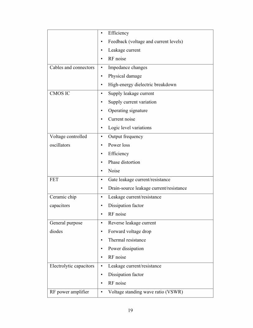
Born and Boenning, [34] and Pecht et al., [35] proposed several measurable
parameters that can be used as failure precursors for electronic switching power
supplies, cables and connectors, CMOS integrated circuits, and voltage-controlled
high-frequency oscillators (see Table 1). Testing was conducted to demonstrate the
potential of select parameters to be viable for detection of incipient failures in
electronic systems.
Table 1. Potential failure precursors for electronics
Electronic Subsystem Failure Precursor Parameter
Switching power
supply
• DC output (voltage and current levels)
• Ripple
• Pulse width duty cycle
19
• Efficiency
• Feedback (voltage and current levels)
• Leakage current
• RF noise
Cables and connectors • Impedance changes
• Physical damage
• High-energy dielectric breakdown
CMOS IC • Supply leakage current
• Supply current variation
• Operating signature
• Current noise
• Logic level variations
Voltage controlled
oscillators
• Output frequency
• Power loss
• Efficiency
• Phase distortion
• Noise
FET • Gate leakage current/resistance
• Drain-source leakage current/resistance
Ceramic chip
capacitors
• Leakage current/resistance
• Dissipation factor
• RF noise
General purpose
diodes
• Reverse leakage current
• Forward voltage drop
• Thermal resistance
• Power dissipation
• RF noise
Electrolytic capacitors • Leakage current/resistance
• Dissipation factor
• RF noise
RF power amplifier • Voltage standing wave ratio (VSWR)

20
• Power dissipation
• Leakage current
Supply current monitoring is routinely performed for testing of CMOS ICs.
This method is based upon the notion that defective circuits produce an abnormal or
at least significantly different amount of current than the current produced by fault-
free circuits. This excess current can be sensed to detect faults. The power supply
current (Idd) can be defined by two elements: the Iddq-quiescent current and the Iddt-
transient or dynamic current. Iddq is the leakage current drawn by the CMOS circuit
when it is in a stable (quiescent) state. Iddt is the supply current produced by circuits
under test (CUT) during a transition period after the input has been applied. Iddq has
been reported to have the potential for detecting defects such as bridging, opens, and
parasitic transistor defects. Operational and environmental stresses such as
temperature, voltage, and radiation can quickly degrade previously undetected faults
and increase the leakage current (Iddq). There is extensive literature on Iddq testing,
but only little has been done on using Iddq for in-situ PHM. Monitoring Iddq has
been more popular than monitoring Iddt [36] [37] [38].
Smith and Campbell, [36] developed a quiescent current monitor (QCM) that
can detect elevated Iddq current in real time during operation. The QCM performed
leakage current measurements on every transition of the system clock to get
maximum coverage of the IC in real time. Pecuh, et al., [37] and Xue and Walker,
[38] proposed a low-power built-in current monitor for CMOS devices. In the Pecuh,
et al., study, the current monitor was developed and tested on a series of inverters for

21
simulating open and short faults. Both fault types were successfully detected and
operational speeds of up to 100 MHz were achieved with negligible effect on the
performance of the circuit under test. The current sensor developed by Xue and
Walker enabled Iddq monitoring at a resolution level of 10 pA. The system translated
the current level into a digital signal with scan chain readout. This concept was
verified by fabrication on a test chip.
It has been proposed by GMA Industries [39] [40] [41] to embed molecular
test equipment (MTE) within ICs to enable them to continuously test themselves
during normal operation and to provide a visual indication that they have failed. The
molecular test equipment could be fabricated and embedded within the individual
integrated circuit in the chip substrate. The molecular-sized sensor "sea of needles"
could be used to measure voltage, current, and other electrical parameters, as well as
sense changes in the chemical structure of integrated circuits that are indicative of
pending or actual circuit failure. This research focuses on the development of
specialized doping techniques for carbon nanotubes to form the basic structure
comprising the sensors. The integration of these sensors within conventional IC
circuit devices, as well as the use of molecular wires for the interconnection of sensor
networks, is an important factor in this research. However, no product or prototype
has been developed to date.
Kanniche and Mamat-Ibrahim, [42] developed an algorithm for health
monitoring of pulse width modulation - voltage source inverters. The algorithm was

22
designed to detect and identify transistor open circuit faults and intermittent misfiring
faults occurring in electronic drives. The mathematical foundations of the algorithm
were based on discrete wavelet transform (DWT) and fuzzy logic (FL). Current
waveforms were monitored and continuously analyzed using DWT to identify faults
that may occur due to constant stress, voltage swings, rapid speed variations, frequent
stop/start-ups, and constant overloads. After fault detection, “if-then” fuzzy rules
were used for VLSI fault diagnosis to pinpoint the fault device. The algorithm was
demonstrated to detect certain intermittent faults under laboratory experimental
conditions.
Lall, et al. [43] [44] have developed a damage pre-cursor based residual life
computation approach for various package elements to prognosticate electronic
systems prior to the appearance of any macro-indicators of damage. In order to
implement the system-health monitoring, precursor variables have been identified for
various package elements and failure mechanisms. Model-algorithms have been
developed to correlate precursors with impending failure for computation of residual
life. Package elements investigated include, first-level interconnects, dielectrics, chip
interconnects, underfills and semiconductors. Examples of damage proxies include,
phase growth rate of solder interconnects, intermetallics, normal stress at chip
interface, and interfacial shear stress. Lall et al., suggest that the pre-cursor based
damage computation approach eliminates the need for knowledge of prior or posterior
operational stresses and enables the management of system reliability of deployed
non-pristine materials under unknown loading conditions. The approach can be used

23
on re-deployed parts, sub-systems and systems, since it does not depend on
availability of prior stress histories.
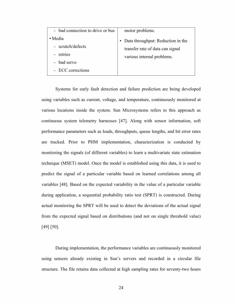
Self-monitoring analysis and reporting technology (SMART) currently
employed in select computing equipment for hard disk drives (HDD) is another
example of precursor monitoring [45] [46]. HDD operating parameters, including the
flying height of the head, error counts, variations in spin time, temperature, and data
transfer rates, are monitored to provide advance warning of failures (see Table 2).
This is achieved through an interface between the computer’s start-up program
(BIOS) and the hard disk drive.
Table 2. Monitoring parameters based on reliability concerns in hard drives
Reliability Issues Parameters Monitored
• Heads/head assembly
- crack on head
- head contamination or
resonance
- bad connection to electronics
module
• Motors/bearings
- motor failure
- worn bearing
- excessive run-out
- no spin
• Electronic module
- circuit/chip failure
- interconnection/solder joint
failure
• Head flying height: A downward
trend in flying height will often
precede a head crash.
• Error Checking and Correction
(ECC) use and error counts: The
number of errors encountered by the
drive, even if corrected internally,
often signals problems developing
with the drive.
• Spin-up time: Changes in spin-up
time can reflect problems with the
spindle motor.
• Temperature: Increases in drive
temperature often signal spindle
24
- bad connection to drive or bus
• Media
- scratch/defects
- retries
- bad servo
- ECC corrections
motor problems.
• Data throughput: Reduction in the
transfer rate of data can signal
various internal problems.
Systems for early fault detection and failure prediction are being developed
using variables such as current, voltage, and temperature, continuously monitored at
various locations inside the system. Sun Microsystems refers to this approach as
continuous system telemetry harnesses [47]. Along with sensor information, soft
performance parameters such as loads, throughputs, queue lengths, and bit error rates
are tracked. Prior to PHM implementation, characterization is conducted by
monitoring the signals (of different variables) to learn a multivariate state estimation
technique (MSET) model. Once the model is established using this data, it is used to
predict the signal of a particular variable based on learned correlations among all
variables [48]. Based on the expected variability in the value of a particular variable
during application, a sequential probability ratio test (SPRT) is constructed. During
actual monitoring the SPRT will be used to detect the deviations of the actual signal
from the expected signal based on distributions (and not on single threshold value)
[49] [50].
During implementation, the performance variables are continuously monitored
using sensors already existing in Sun’s servers and recorded in a circular file
structure. The file retains data collected at high sampling rates for seventy-two hours
25
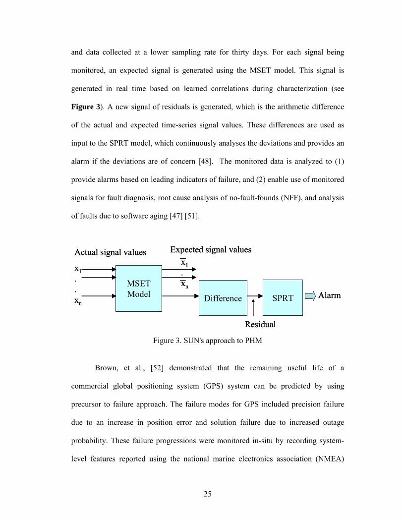
and data collected at a lower sampling rate for thirty days. For each signal being
monitored, an expected signal is generated using the MSET model. This signal is
generated in real time based on learned correlations during characterization (see
Figure 3). A new signal of residuals is generated, which is the arithmetic difference
of the actual and expected time-series signal values. These differences are used as
input to the SPRT model, which continuously analyses the deviations and provides an
alarm if the deviations are of concern [48]. The monitored data is analyzed to (1)
provide alarms based on leading indicators of failure, and (2) enable use of monitored
signals for fault diagnosis, root cause analysis of no-fault-founds (NFF), and analysis
of faults due to software aging [47] [51].
Figure 3. SUN's approach to PHM
Brown, et al., [52] demonstrated that the remaining useful life of a
commercial global positioning system (GPS) system can be predicted by using
precursor to failure approach. The failure modes for GPS included precision failure
due to an increase in position error and solution failure due to increased outage
probability. These failure progressions were monitored in-situ by recording system-
level features reported using the national marine electronics association (NMEA)
MSETModel Difference SPRT Alarm
Residual
Expected signal valuesActual signal values
x1..xn
x1.xnMSET
Model Difference SPRT Alarm
Residual
Expected signal valuesActual signal values
x1..xn
x1.xn

26
protocol 0183. The GPS was characterized to collect the principal feature value for a
range of operating conditions. The approach was validated by conducting accelerated
thermal cycling of the GPS with the offset of the principal feature value measured in-
situ. Based on experimental results, parametric models were developed to correlate
the offset in the principal feature value with solution failure. During the experiment
the BIT provided no indication of an impending solution failure [52].
In general to implement a precursor reasoning-based PHM system, it is
necessary to identify the precursor variables for monitoring, and then develop a
reasoning algorithm to correlate the change in the precursor variable with the
impending failure. This characterization is typically performed by measuring the
precursor variable under an expected or accelerated usage profile. Based on the
characterization, a model is developed - typically a parametric curve-fit, neural-
network, Bayesian network, or a time-series trending of a precursor signal. This
approach assumes that there is one or more expected usage profiles that are
predictable and can be simulated in a laboratory setup. In some products the usage
profiles are predictable, but this is not always true.
For a fielded product with highly varying usage profiles, an unexpected
change in the usage profile could result in a different (non-characterized) change in
the precursor signal. If the precursor reasoning model is not characterized to factor in
the uncertainty in life-cycle usage and environmental profiles, it may provide false
alarms. Additionally, it may not always be possible to characterize the precursor

27
signals under all possible usage scenarios (assuming they are known and can be
simulated). Thus, the characterization and model development process can often be
time-consuming and costly and may not work.
2.4 Monitoring Environmental and Usage Loads
The life-cycle environment of a product consists of manufacturing, storage,
handling, operating and non-operating conditions. The life-cycle loads (Table 3),
either individually or in various combinations, may lead to performance or physical
degradation of the product and reduce its service life [53]. The extent and rate of
product degradation depends upon the magnitude and duration of exposure (usage
rate, frequency, and severity) to such loads. If one can measure these loads in-situ, the
load profiles can be used in conjunction with damage models to assess the
degradation due to cumulative load exposures.
Table 3. Examples of life-cycle loads Load Load Conditions
Thermal Steady-state temperature, temperature ranges, temperature
cycles, temperature gradients, ramp rates, heat dissipation
Mechanical Pressure magnitude, pressure gradient, vibration, shock load,
acoustic level, strain, stress
Chemical Aggressive versus inert environment, humidity level,
contamination, ozone, pollution, fuel spills
Physical Radiation, electromagnetic interference, altitude
Electrical Current, voltage, power

28
The assessment of the impact of life-cycle usage and environmental loads on
electronic structures and components was studied by Ramakrishnan and Pecht [53].
This study introduced the life consumption monitoring (LCM) methodology (Figure
4), which combined in-situ measured loads with physics-based stress and damage
models for assessing the life consumed.
Figure 4. CALCE life consumption monitoring methodology
The application of the LCM methodology to electronics PHM was illustrated
with two case studies [53] [54]. The test vehicle consisted of an electronic
component-board assembly placed under the hood of an automobile and subjected to
normal driving conditions in the Washington, DC, area. The test board incorporated
eight surface-mount leadless inductors soldered onto an FR-4 substrate using eutectic
tin-lead solder. Solder joint fatigue was identified as the dominant failure
Step 1: Conduct failure modes, mechanisms and effects analysis
Step 6: Estimate the remaining life of the product
Step 5: Perform stress and damage accumulation analysis
Continue monitoring
Is the remaining-life
acceptable?
No
Yes
Step 4: Conduct data simplification to make sensor data suitable for stress and damage models
Schedule a maintenance action
Step 3: Monitor appropriate product parametersenvironmental (e.g, shock, vibration, temperature, humidity)
operational (e.g., voltage, power, heat dissipation)
Step 2: Conduct a virtual reliability assessment to assess the failure mechanisms with earliest time-to-failure
Step 1: Conduct failure modes, mechanisms and effects analysis
Step 6: Estimate the remaining life of the product
Step 5: Perform stress and damage accumulation analysis
Continue monitoring
Is the remaining-life
acceptable?
Is the remaining-life
acceptable?
No
Yes
Step 4: Conduct data simplification to make sensor data suitable for stress and damage models
Schedule a maintenance action
Step 3: Monitor appropriate product parametersenvironmental (e.g, shock, vibration, temperature, humidity)
operational (e.g., voltage, power, heat dissipation)
Step 2: Conduct a virtual reliability assessment to assess the failure mechanisms with earliest time-to-failure

29
mechanism. Temperature and vibrations were measured in-situ on the board in the
application environment. Using the monitored environmental data, stress and damage
models were developed and used to estimate consumed life. The LCM methodology
accurately predicted remaining life.
Mathew, et al., [55] applied the LCM methodology in conducting a prognostic
remaining-life assessment of circuit cards inside a space shuttle solid rocket booster
(SRB). Vibration time history recorded on the SRB from the pre-launch stage to
splashdown were used in conjunction with physics-based models to assess the
damage caused due to vibration and shock loads. Using the entire life-cycle loading
profile of the SRBs, the remaining life of the components and structures on the circuit
cards were predicted. It was determined that an electrical failure was not expected
within another forty missions. However, vibration and shock analysis exposed an
unexpected failure of the circuit card due to a broken aluminum bracket mounted on
the circuit card. Damage accumulation analysis determined that the aluminum
brackets had lost significant life due to shock loading.
Shetty, et al. [56] applied the LCM methodology for conducting a prognostic
remaining-life assessment of the end effector electronics unit (EEEU) inside the
robotic arm of the space shuttle remote manipulator system (SMRS). A life-cycle
loading profile for thermal and vibrational loads was developed for the EEEU boards.
Damage assessment was conducted using physics-based mechanical and
thermomechanical damage models. A prognostic estimate using a combination of

30
damage models, inspection, and accelerated testing showed that there was little
degradation in the electronics and they could be expected to last another twenty years.
Vichare, et al. [2] [57] outlined generic strategies for in-situ load monitoring,
including selecting appropriate parameters to monitor and designing an effective
monitoring plan. Methods for processing the raw sensor data during in-situ
monitoring to reduce the memory requirements and power consumption of the
monitoring device were presented. Approaches were also presented for embedding
intelligent front-end data processing capabilities in monitoring systems to enable data
reduction and simplification (without sacrificing relevant load information) prior to
input in damage models for health assessment and prognostics.
Embedding the data reduction and load parameter extraction algorithms in to
the sensor modules as suggested by Vichare et al., [57] can lead to reduction in on-
board storage space, low power consumption, and uninterrupted data collection over
longer durations. A time-load signal can be monitored in-situ using sensors, and
further processed to extract (in this case) cyclic range (∆s), cyclic mean load (Smean),
and rate of change of load (ds/dt) using embedded load extraction algorithms. The
extracted load parameters can be stored in appropriately binned histograms to achieve
further data reduction. After the binned data is downloaded, it can be used to
estimate the distributions of the load parameters. The usage history is used for
damage accumulation and remaining life prediction.

31
Efforts to monitor life-cycle load data on avionics modules can be found in
time-stress measurement device (TSMD) studies. Over the years the TSMD designs
have been upgraded using advanced sensors [58], and miniaturized TSMDs are being
developed due to advances in microprocessor and non-volatile memory technologies
[59].
Searls, et al., [60] undertook in-situ temperature measurements in both
notebook and desktop computers used in different parts of the world. In terms of the
commercial applications of this approach, IBM has installed temperature sensors on
hard drives (Drive-TIP) [61] to mitigate risks due to severe temperature conditions,
such as thermal tilt of the disk stack and actuator arm, off-track writing, data
corruptions on adjacent cylinders, and outgassing of lubricants on the spindle motor.
The sensor is controlled using a dedicated algorithm to generate errors and control fan
speeds.
Strategies for efficient in-situ health monitoring of notebook computers were
provided by Vichare, et al., [62]. In this study the authors monitored and statistically
analyzed the temperatures inside a notebook computer, including those experienced
during usage, storage, and transportation, and discussed the need to collect such data
both to improve the thermal design of the product and to monitor prognostic health.
The temperature data was processed using two algorithms: (1) ordered overall range
(OOR) to convert an irregular time-temperature history into peaks and valleys and
also to remove noise due to small cycles and sensor variations, and (2) a three-

32
parameter Rainflow algorithm to process the OOR results to extract full and half
cycles with cyclic range, mean and ramp rates. The effects of power cycles, usage
history, CPU computing resources usage, and external thermal environment on peak
transient thermal loads were characterized.
The European Union funded a project from September 2001 through February
2005 named environmental life-cycle information management and acquisition for
consumer products (ELIMA), which aimed to develop ways of better managing the
life cycles of products using technology to collect vital information during a product’s
life to lead to better and more sustainable products [63] [64]. Though the focus of this
work was not on prognostics, the project demonstrated the monitoring of the life-
cycle conditions of electronic products by field trials. ELIMA partners built and
tested two special prototype consumer products with data collection features, and
investigated the implications for producers, users, and recyclers. The ELIMA
technology included sensors and memory built into the product to record dynamic
data such as operation time, temperature, and power consumption. This was added to
static data about materials and manufacture. Both a direct communication (via GSM
module) as well as a two-step communication with the database (RFID data retrieval
followed by an Internet data transfer) was applied. As a case study, the member
companies monitored the application conditions of a game console and a household
fridge-freezer.

33
Skormin, et al., [65] developed a data mining model based for failure
prognostics of avionics units. The model provides a means of efficiently clustering
data on parameters measured during operation, such as vibration, temperature, power
supply, functional overload, and air pressure. These parameters are monitored in-situ
on the flight using time-stress measurement devices. The objectives of the model are
(1) to investigate the role of measured environmental factors in the development of
particular failure; (2) to investigate the role of combined effects of several factors;
and (3) to reevaluate the probability of failure on the basis of known exposure to
particular adverse conditions. Unlike the physics-based assessments made by
Ramakrishnan and Pecht [53], the data mining model relies on the statistical data
available from the records of a time-stress measurement device (TSMD) on
cumulative exposure to environmental factors and operational conditions. The TSMD
records, along with calculations of probability of failure of avionics units, are used for
developing the prognostic model. The data mining enables an understanding of the
usage history and allows tracing the cause of failure to individual operational and
environmental conditions.
2.5 PHM Integration
Implementing an effective PHM strategy for an entire system will involve
integrating different health monitoring approaches. An extensive analysis may be
required to determine the weak link(s) in the system to enable a more focused
monitoring process. Once the potential failure modes, mechanisms, and effects have
been identified, a combination of BIT, canaries, precursor reasoning, and life-cycle

34
damage modeling may be necessary, depending on the failure attributes. In fact,
different approaches can be implemented based on the same sensor data. For
example, operational loads, such as temperature, voltage, supply current, and
acceleration, can be collected by BIT. The current and temperature data can be used
with damage models to calculate the susceptibility to electromigration between
metallizations. Also, the supply-current data can be used with precursor reasoning
algorithms for identifying signs of transistor degradation.
Case studies of the integration of different approaches of PHM can be found
in work by CALCE [66] [56] and R. Orsagh, et al., [67], which used physics-based
models for damage accumulation and precursor reasoning for system assessment. A
detailed FMMEA [33] was conducted and time to failure was assessed for the failure
mechanisms identified by the FMMEA using appropriate failure models. The time-to-
failures were ranked and a risk assessment was made based on severity and
occurrence before PHM implementation [66]. In another PHM study [68], an off-the-
shelf 50-watt, DC-to-DC converter from a commercial power supply manufacturer
was used. As in the CALCE studies [66] [56], a detailed a-priori analysis of power
supply reliability issues was conducted in this case using the Pareto analysis of
failures reported by the manufacturer. PHM techniques were then aimed at
monitoring and predicting the most common failures.
Future electronic system designs will integrate sensing and processing
modules that will enable in-situ PHM. Advances in sensors, microprocessors,

35
compact non-volatile memory, battery technologies, and wireless telemetry have
already enabled the implementation of sensor modules and autonomous data loggers.
For in-situ health monitoring, integrated, miniaturized, low-power, reliable sensor
systems operated using portable power supplies (such as batteries) are being
developed. These sensor systems have self-contained architecture requiring minimum
or no intrusion into the host product in addition to specialized sensors for monitoring
localized parameters. Sensors with embedded algorithms will enable fault detection,
diagnostics, and remaining life prognostics that would ultimately drive the supply
chain. The prognostic information will be linked via wireless communications to
relay needs to maintenance officers and automatic identification techniques (RFID
being the most common current example) will be used to locate parts in the supply
chain--all integrated through a secure web portal to acquire and deliver replacement
parts quickly on an as-needed basis.

36
Chapter 3: Prognostics Using Environmental and Usage Loads
3.0 Introduction
This chapter presents the prognostic approach that is based on accumulating
damage due to environmental and usage exposures. This chapter discusses the
approach and its implementation setup for electronic prognostics used in this
research. The key challenges in implementing this approach are presented. These
challenges and proposed solutions will be discussed in more details in individual
chapters.
3.1 Approach
The basic philosophy underlying the type of PHM approach is that damage is
a function of the loads experienced by the product in the life cycle environment. The
life cycle environment of a product consists of manufacturing, storage, handling,
operating and non-operating scenario. The life cycle loads consists of thermal
(steady-state temperature, temperature ranges, temperature cycles, temperature
gradients), mechanical (pressure levels, pressure gradients, vibrations, shock loads,
acoustic levels), chemical (aggressive or inert environments, humidity levels,
contamination), physical (radiation, electromagnetic interference, altitude),
environmental (ozone, pollution, fuel spills) and usage loads (usage frequency, usage
severity, usage time, power, heat dissipation, current, voltage etc.) [2] [57]. These
loads either individually or in various combinations may lead to performance or
physical degradation of the product and subsequently reduce its service life. The

37
extent and rate of product degradation depends upon the nature, magnitude, and
duration of exposure to such loads
For implementation of this approach, strategies are required to design an
effective PHM process for the product and application specific needs. Environmental
and usage load profiles need to be efficiently and accurately captured in the
application environment, and utilized in real time or near real time health assessment
and prognostics. It is essential to simplify or pre-process the “raw” sensor data to
make it compatible with the damage models and algorithms needed to conduct
prognostics. In particular, it may be necessary to extract the relevant load parameters
including cyclic mean, amplitudes, ramp rates, hold periods, power spectral densities,
etc. Commonly used load parameter extraction methods include: cycle counting
algorithms for extracting cycles from time-load signal, Fast Fourier transforms (FFT)
for extracting the frequency content of signals, etc. Depending on the application and
type of signal, custom load extraction methods may be required.
Figure 5 is a schematic of the in-situ monitoring, pre-processing, and storage
of environmental and usage loads. A time-temperature signal is monitored in-situ
using sensors, and further processed to extract (in this case) cyclic temperature range
(∆T), cyclic mean temperature (Tmean), ramp rate (dT/dt), and dwell time (tD) using
embedded load extraction algorithms. The extracted load parameters are stored in
appropriate bins to achieve further data reduction. The binned data is downloaded to
estimate the distributions of the load parameters for use in damage assessment,
remaining life estimation, and the accumulation of the products use history.

38
Figure 5. Prognostic approach using environmental and usage loads
Once these load parameters are obtained, they can then be used in conjunction
with damage models in Table 4 to assess the damage at various failure sites due to
different failure mechanisms for a given electronic assembly. A comprehensive
listing of loads, models, and failure mechanisms can be found in the following
documents JESD659-A: Failure-mechanism-driven reliability monitoring, JEP143A:
Solid-state reliability assessment and qualification methodologies, JEP150: Stress-
test-driven qualification of and failure mechanisms associated with assembled solid
state surface-mount components, JESD94: Application specific qualification using
knowledge based test methodology, JESD91A: Method for developing acceleration
models for electronic component failure mechanisms, SEMATECH, #00053955A-
XFR: Semiconductor device reliability failure models, SEMATECH, #00053958A-
XFR: Knowledge-based reliability qualification testing of silicon devices, and
,.....),,,( Dmean tdtdTTTfw ∆=∆Damage,
Time (t)
Tem
pera
ture
(T)
Embedded Data Reduction and Load Parameter Extraction
Remaining life = f (Σ ∆w)
Mean (Tmean) Ramp rate (dT/dt)0
0.25
0.5
Range (∆T)
Freq
uenc
y
Dwell time (tD)0
0.25
0.5
0
0.25
0.5
0
0.25
0.5
,.....),,,( Dmean tdtdTTTfw ∆=∆Damage,
Time (t)
Tem
pera
ture
(T)
Embedded Data Reduction and Load Parameter Extraction
Remaining life = f (Σ ∆w)
Mean (Tmean) Ramp rate (dT/dt)0
0.25
0.5
Range (∆T)
Freq
uenc
y
Dwell time (tD)0
0.25
0.5
0
0.25
0.5
0
0.25
0.5
Mean (Tmean) Ramp rate (dT/dt)0
0.25
0.5
0
0.25
0.5
Range (∆T)
Freq
uenc
y
Dwell time (tD)0
0.25
0.5
0
0.25
0.5
0
0.25
0.5
0
0.25
0.5
0
0.25
0.5
0
0.25
0.5
0
0.25
0.5

39
SEMATECH, #99083810A-XFR: Use condition based reliability evaluation of new
semiconductor technologies [69] [70].
Table 4. Failure mechanisms, relevant loads, and models in electronics Failure Mechanisms Failure Sites Relevant Loads Sample Models
Fatigue Die attach, Wirebond/TAB, Solder leads, Bond pads, Traces, Vias/PTHs, Interfaces
∆ T, Tmean, dT/dt, dwell time, ∆H, ∆V
Nonlinear Power Law (Coffin-Manson)
Corrosion Metallizations M, ∆V, T Eyring (Howard) Electromigration Metallization T, J Eyring (Black) Conductive Filament Formation
Between Metallization M, ∇ V Power Law (Rudra)
Stress Driven Diffuison Voiding
Metal Traces s, T Eyring (Okabayashi)
Time Dependant Dielectric Breakdown
Dielectric layers V, T Arrhenius (Fowler-Nordheim)
∆: Cyclic range ∇ : gradient
V: Voltage M: Moisture
T: Temperature J:Current density
s: Stress H: Humidity
3.2 Implementation Setup
The experiment was setup to implement the PHM methodology based on
damage accumulation due to environmental and usage exposures for predicting
remaining life of solder joint interconnects under temperature cycling loads. An
electronic test board was exposed to a completely irregular temperature profile. The
test board used for this research is shown in Figure 6. The board contains 12 surface
mount components soldered on a 62 mil thick high Tg FR-4 substrate using eutectic
Sn-Pb solder. The components are dummy packages with small size silicon die. All
components are daisy chained to facilitate continuity monitoring during testing. A
daisy chain is a conductive path that connects several interconnections of a
40
component. In this experiment a failure (refer to failure definitions in the main
document) of any daisy chain indicates the failure of the component. The overall
dimensions of the board are 8” X 5.5” and the pad finish is immersion silver
The profile simulated field conditions by exposing the board to random
temperature variations similar to those experienced due to random usage. This profile
was generated in a programmable oven, such that each successive profile has
completely different peak temperatures, ramp rates, and dwell times. The
environmental chamber used for this work was the Thermatron 2800 S1.2, which is
capable of storing 255 discrete time-temperature intervals and sequencing them in
different loops. An example of the temperature profile for the first 20 days is shown
in Figure 7. During testing, the temperatures at various locations of the board were
measured in-situ using sensors placed on the board. The temperature was monitored
every 10 seconds. Two instruments were used, one is a prototype miniature sensing
and data recording systems (HUMS) provided by European Aeronautics and Defense
Space (EADS) systems. However, for most part of the experiment, a multi-channel
data logger (from Agilent) with multiplexing units was used.
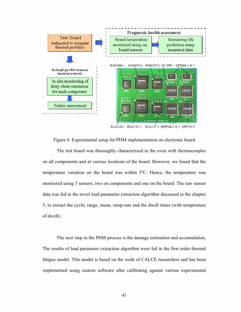
41
Figure 6. Experimental setup for PHM implementation on electronic board
The test board was thoroughly characterized in the oven with thermocouples
on all components and at various locations of the board. However, we found that the
temperature variation on the board was within 5oC. Hence, the temperature was
monitored using 3 sensors, two on components and one on the board. The raw sensor
data was fed in the novel load parameter extraction algorithm discussed in the chapter
5, to extract the cyclic range, mean, ramp-rate and the dwell times (with temperature
of dwell).
The next step in the PHM process is the damage estimation and accumulation.
The results of load parameter extraction algorithm were fed in the first order thermal
fatigue model. This model is based on the work of CALCE researchers and has been
implemented using custom software after calibrating against various experimental

42
studies. Using this thermal fatigue model and the board and component specific
information on material properties and geometry, the model was used to assess the
damage of solder joints on the test board. The model has been used extensively for
calculating solder fatigue and provides rapid assessment which makes it more
attractive for in-situ assessments for PHM application.
The package geometries namely, the size, shape, and areas of the solder balls
and the gull wing interconnects were supplied by the manufacturer. Some of these
values were verified by actual measurement. The material properties of solder, board,
interconnect, and packages were obtained from the manufacturer. For routinely used
materials such as Pb-Sn solder, and FR-4, these properties are stored in the database
of the CalcePWA software that was used for building the model. These properties
have been derived from several experimental results and from literature.
Figure 7. Illustration of temperature measured on the board for first 20 days

43
Prior to exposing the test board to irregular cycles, another board of the exact
same design was exposed to constant thermal cycling profile ranging from -40oC to
125oC, with a 15 minute and 10 minute dwell at maximum and minimum
temperatures. The temperature ramp-up and ramp-down rate was set at 5.5oC/minute
and 8.5oC/minute. The accuracy of the damage model was assessed by comparing the
model predictions with results from testing to actual failure due to temperature
cycling. Additionally, a range of different thermal cycling conditions were simulated.
The results from testing were compared with modeling. Four thermal cycling
parameters namely the temperature amplitude (∆T), cyclic mean temperature (Ts),
ramp rate from low to high temperatures, and dwell time at high temperature (tD),
were studied and the impact of each parameter on the life of solder joints was
assessed by sensitivity studies.
The thermal-fatigue model provides a damage fraction due to each thermal
cycle exposure, which is accumulated linearly using Miner’s hypothesis. The damage
fraction greater than or equal to 1 indicates failure or end of life of the product being
monitored. Along with the temperature, the daisy chain resistance (actual electrical
performance) of the solder interconnects is measured in-situ. The failure criteria for
the solder joints was set as per IPC standard IPC-SM 785 [71], that states that failure
manifests itself in form of resistance spikes of short durations >300 Ω and failure is
defined as the first interruption of electrical continuity that is confirmed by 9
additional interruptions with an additional 10% of cycle life. The failure of the solder
joints obtained from the resistance measurement indicates the actual failure. The

44
actual (measured) failure of the solder joint is compared with the prediction made
using PHM (temperature measurement and damage accumulation) to validate the
PHM methodology. The details of damage assessment and life prediction will be
presented in chapter six.
3.3 Summary
The prognostic approach based on monitoring and modeling of environmental
and usage loads was presented. The experimental setup for demonstrating the PHM
technique for an electronic board was discussed. The temperature data from this
experiment was used for demonstrating the load parameter extraction algorithm and
the method for optimal binning (chapter 5). Also, the temperature data was used with
damage models for enabling prognostics of solder joints in thermal cycling (Chapter
6). Finally, the in-situ resistance measurements, along with the temperature were used
for identification and trending of failure precursors (chapter 7).

45
Chapter 4: Methods for In-situ Monitoring
4.0 Introduction
A major challenge in PHM is its implementation in the application
environment. Strategies are required to design an effective PHM process for the
product and application specific needs. Environmental and usage load profiles need
to be efficiently and accurately captured in the application environment, and utilized
in real time or near real time health assessment and prognostics. This paper outlines
generic strategies both for load monitoring and conversion of the sensor data into a
format that can be used in physics-of-failure models, for both damage estimation and
remaining life prediction due to specific failure mechanisms. The selection of
appropriate parameters to monitor, design of an effective monitoring plan, and
selection of appropriate monitoring equipment are discussed. Methods to process the
raw sensor data during in-situ monitoring for reducing the memory requirements and
power consumption of the monitoring device are suggested. Conceptual approaches
are also presented for embedding such processing capabilities in monitoring systems
to enable data reduction and simplification (without sacrificing relevant load
information) prior to model input for health assessment and prognostics. The
strategies presented are generically applicable to electronic health monitoring
processes and are illustrated using a case-study of in-situ monitoring of a note-book
computer.

46
4.1 In-situ Monitoring of Environmental and Usage Loads
The requirements for data collection may be well known or already specified
for some applications. However, in many applications, it is not always à priori
known what parameters need to be measured, nor with what frequency or precision.
It may be useful to conduct preliminary field tests and collect additional data that may
not be justified in a fully operating system, so as to understand what data is actually
relevant. If the objective of data collection is for use in an ongoing product design
phase, the aim would be to gather maximum data in a minimum time frame. For
health assessment as well as design decisions, monitoring plans are required to
capture the distribution of loading parameters and usage profiles. The life cycle loads
further depend on the usage conditions such as usage frequency, severity, and period
of use. The following sections outline the steps in implementing a process for
effective monitoring of life cycle loads.
4.1.1 Selection of Load Parameters for Monitoring
The first step in the data collection process is to select the life cycle
parameters to be monitored. Parameters can be identified based on factors that are
crucial for safety, are likely to cause catastrophic failures, are essential for mission
completeness, or can result in long downtimes. Selection can also be based on
knowledge of the critical parameters established from past experience and field
failure data on similar products, and qualification testing. More systematic methods
such as failure mode and effects analysis (FMEA) or failure mode mechanisms and
effects analysis (FMMEA) [33] can be used to determine parameters that need to be
monitored.

47
Table 4 (previous chapter) provides a listing of common failure mechanisms
in electronics with the relevant loads and associated models compiled from JEDEC
standards JEP122B (Failure Mechanisms and Models for Semiconductor Device) and
JEP 148 (Reliability Qualification of Semiconductor Devices Based on Physics of
Failure Risk and Opportunity Assessment). The failure mechanisms and models can
serve as a starting point for selecting the appropriate parameters.
4.1.2. Selection of Monitoring Equipment
The main attributes of a sensor system for environmental and usage
monitoring include level of integration, power consumption and management, on-
board memory and utilization, size and weight, wireless communication, embedded
computational power, software support, and product maturity. Each attribute is
discussed in detail below.
Level of Integration
A completely integrated sensor system consists of the sensing elements, on-
board analog to digital converter, on-board memory, embedded computational
capabilities, ability to communicate with other sensor nodes, and completely
supported by indigenous power supply. For in-situ monitoring, the requirements for
data collection may be well known or already specified for some applications.
However, in many applications, it is not always a-priori known what parameters need
to be measured, nor with what frequency or precision. Hence, sensor systems with
modular architecture consisting of integrated core central nodes and easy add-on
nodes are preferred.

48
Sensor systems for environmental monitoring need to be a self-contained,
requiring minimum or no intrusion into the host product. This can facilitate
monitoring of legacy systems without the need for any testing or qualification.
Flexible sensor ports that support a wide variety of sensors (such as ports for all
sensors with input requirements between 0-3V) are preferred over rigid customized
ports (such as ports designed specifically for particular sensor types say
thermocouples). An example of integrated sensor system is shown Figure 8.
Figure 8. Conceptual schematic of integrated sensor system
Autonomous Power and Power Management Features
One of the major constraints that strongly influences the selection of
components and hence the size, weight, and cost of the monitoring system is power
consumption. The power consumption of sensor systems can be divided into three
domains: sensing, communication, and processing. The power consumed for sensing
Exte
rnal
Sen
sor M
odul
e
Internal Sensors
External battery
Non-Volatile Memory
(Data Storage)
Flash Memory
(Embedded Software)
Tran
scei
ver Handheld
device
Base Station PC
Low power 8-bit
High power 32-bit
Microcontroller (with ADC)
RFI
D
Exte
rnal
Sen
sor M
odul
e
Internal Sensors
External battery
Non-Volatile Memory
(Data Storage)
Non-Volatile Memory
(Data Storage)
Flash Memory
(Embedded Software)
Flash Memory
(Embedded Software)
Tran
scei
ver
Tran
scei
ver Handheld
device
Base Station PC
Handheld device
Base Station PC
Low power 8-bit
High power 32-bit
Microcontroller (with ADC)
RFI
D

49
varies depending on the parameter being monitored. Periodic sensing can consume
less power than continuous monitoring; however there is a risk of missing important
data. Power consumption is also controllable by making measurements at events
triggered by defined thresholds. The need for power management is even more
challenging in wireless sensor systems running on batteries. In the case of wireless
sensors, maximum energy is expended in communication, which involves both the
data transmission and reception.
On- board Memory and Utilization
Effective utilization of memory is also an important attribute in setting up the
sensor system. Memory requirements are affected by the monitoring interval and
frequency. In selecting the monitoring frequency, the user has to ensure that the
relevant loads are recorded and, at the same time, the memory is not flooded by
irrelevant load data. The user should be able to define threshold values for
measurement. Appropriate setting of thresholds can facilitate efficient data
collection. For example, measurements can be recorded or a scan can be triggered
only if the stimulus meets the set threshold. Events can be set to trigger above or
below an absolute value, for example, recording acceleration levels above 2g or
humidity levels above 80% R.H. Users can also set thresholds based on the value of
the slope (positive or negative) of the curve formed by the measurements made by the
sensor. This strategy allows usage-based data recording, which can result in a
substantial saving in disk space and extend the battery life of the equipment. Other
means of memory utilization involve effectively dividing the memory between

50
periodic measurements and threshold based measurements. A strategic combination
of measurement intervals (for periodic measurements) and thresholds can enable
recording a higher number of relevant measurements.
Miniature Size and Low Weight
In some applications, the size of the sensor may become the significant
selection criteria due to limited space available for mounting the sensor or due to the
inaccessibility of locations to be sensed. The weight of the sensor may be important
in certain applications such as vibration and shock measurements using
accelerometers, since the added mass can change the system response. In the case
where a fixture is required to mount the sensor, the added mass of the sensor and
fixture may change the system characteristics. Users should consider the entire
weight of the sensor system, which includes the battery and other accessories such as
communication antennas and cables.
Wireless Capabilities
Wireless monitoring has emerged in recent years as a promising technology
that can impact in-situ environmental monitoring. Wireless sensor nodes can be used
to remotely monitor inhospitable and toxic environments. In some applications,
sensor(s) must operate remotely with data stored and downloaded by telemetry to a
centrally located processing station. Also, wireless sensor systems are not dependent
on extensive lengths of coaxial wires for the transfer of sensor measurements, thus
saving installation and maintenance costs. The real benefit from wireless sensor

51
nodes can be achieved by embedding micro-controllers with the sensor nodes to
improve the data analysis capabilities within the wireless sensing nodes themselves.
The use of portable devices (such as a PDA) in conjunction with wireless
sensor systems can enable efficient fault diagnosis and prognostics by integrating
more complex algorithms in the hand-held device. Customized processing and
reporting tools can be programmed on portable devices for efficient maintenance
activities. For example, the data collected by a Bluetooth-enabled accelerometer
system can be downloaded on a hand-held device by maintenance technicians and can
be processed further using Fast Fourier Transforms (FFT) embedded on the hand-held
device.
Embedded Computation Capability
Integrating embedded computational capabilities with on-board processors
can reduce the power consumption of wireless sensor systems. These processing
capabilities would enable immediate and localized processing of the raw sensor data.
This in turn enables transmitting fewer amounts of data (processed instead of raw
data) to the base station, and hence results in lower power consumption. In the case
of a large number of sensor systems working in a network, this would allow
decentralization of computational power and facilitate efficient parallel processing of
data.

52
Additionally, embedding computational power with on-board processors can
also facilitate efficient data analysis for environmental monitoring applications.
Embedded computations can be set to provide real time updates for taking immediate
action such as powering off the equipment to avoid accidents or catastrophic failures,
and also for providing prognostic horizons for conducting next repair and
maintenance activities. Power consumption and flash memory of the microprocessor
may limit computationally intensive algorithms to be embedded with on-board
processors. However, even using simple algorithms and routines to process the raw
sensor data significant gains can be achieved for in-situ analysis.
Software Support
Sensor systems need host software that can effectively control and
communicate with the hardware. Host software can include capabilities to guide the
user in selecting measurement scans and thresholds values, communicating with the
sensor module to check operational status, enabling operation based power
management, and trouble-shooting or diagnosing the hardware in case of problems.
Software modules with low memory requirement that can be operated from portable
device such as PDA are advantageous for health monitoring applications. For certain
applications modules for immediate data analysis can be a part of the host software.
4.1.3. Design of Monitoring Plan
The important aspect of the in-situ load monitoring process is the setup of data
collection equipment before dispatching in the application environment. Once the

53
parameters to be monitored are selected the next step is to design the complete
monitoring process. The user needs to select the monitoring equipment (sensors and
data recorders), and setup the monitoring process. The important items in the setup
include deciding the monitoring interval and frequency. In making this decision the
user has to ensure that the relevant loads are recorded and at the same time the
memory is not flooded by irrelevant load data. Table 5 provides a list of challenges
and possible solutions that can guide in setting up the monitoring equipment.
Effective utilization of memory is also an important parameter in setting up
the sensor system. The user should be able to define threshold values for
measurement. Appropriate setting of thresholds can facilitate efficient data
collection. Measurement will be recorded or a scan will be triggered only if the
stimulus meets the set threshold. Events can be set to trigger above or below an
absolute value, for example, recording acceleration levels above 2g or humidity levels
above 80%R.H. Users can also set thresholds based on the value of the slope
(positive or negative) of the curve formed by the measurements made by the sensor.
This strategy allows usage based data recording, which can result in substantial
saving in disk space and extend the battery life of the equipment.
Higher levels of threshold lead to greater abbreviation of the load history.
However, it can also introduce errors in the damage assessment. The monitored loads
are simplified and used as inputs to physics-based models for assessing the damage
and failure susceptibility due to a particular failure mechanism. Hence, the threshold
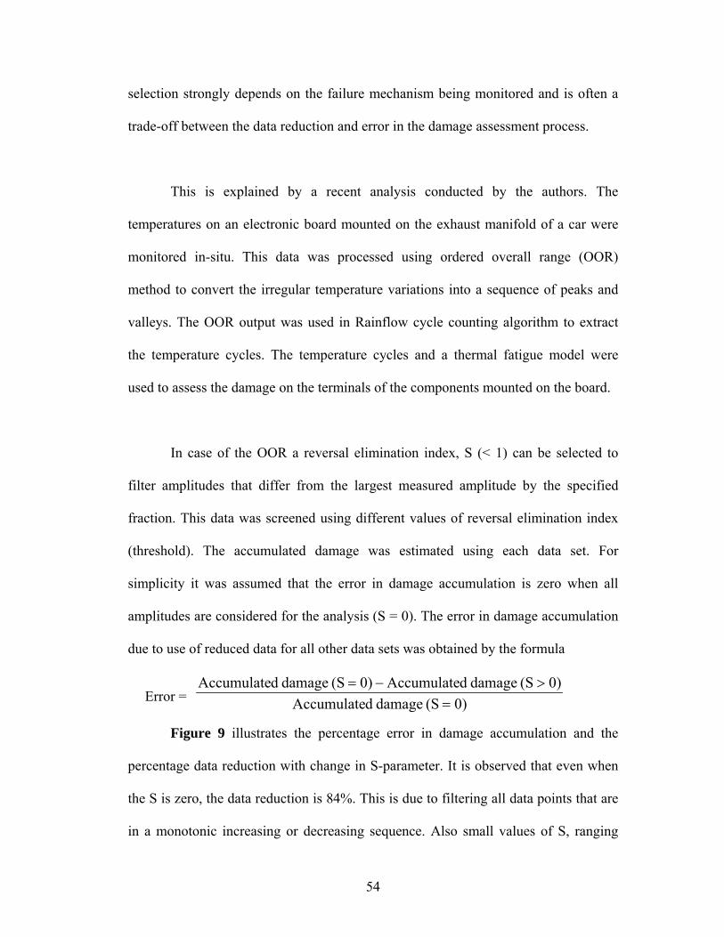
54
selection strongly depends on the failure mechanism being monitored and is often a
trade-off between the data reduction and error in the damage assessment process.
This is explained by a recent analysis conducted by the authors. The
temperatures on an electronic board mounted on the exhaust manifold of a car were
monitored in-situ. This data was processed using ordered overall range (OOR)
method to convert the irregular temperature variations into a sequence of peaks and
valleys. The OOR output was used in Rainflow cycle counting algorithm to extract
the temperature cycles. The temperature cycles and a thermal fatigue model were
used to assess the damage on the terminals of the components mounted on the board.
In case of the OOR a reversal elimination index, S (< 1) can be selected to
filter amplitudes that differ from the largest measured amplitude by the specified
fraction. This data was screened using different values of reversal elimination index
(threshold). The accumulated damage was estimated using each data set. For
simplicity it was assumed that the error in damage accumulation is zero when all
amplitudes are considered for the analysis (S = 0). The error in damage accumulation
due to use of reduced data for all other data sets was obtained by the formula
Error = 0)(S damage dAccumulate0)(S damage dAccumulate0)(S damage dAccumulate
=>−=
Figure 9 illustrates the percentage error in damage accumulation and the
percentage data reduction with change in S-parameter. It is observed that even when
the S is zero, the data reduction is 84%. This is due to filtering all data points that are
in a monotonic increasing or decreasing sequence. Also small values of S, ranging

55
from 0 to 0.1 resulted in more than 90% data reduction with only 1% error in the
damage calculation. Higher values of S result in increasing error in damage
accumulation. This is due to elimination of reversals with large magnitude and the
dependence of the fatigue model on the temperature amplitude.
The answer to the question on selecting the S parameter can be answered by
assessing the distribution of cycles that are obtained after screening the data. Figure
10, compares the number of temperature cycles obtained after processing the data
with S = 0.1 against S = 0. By choosing S value as 0.1, all cycles with amplitude <
15oC are eliminated. It cannot be directly concluded from Figure 10 that all the
temperature cycles with amplitude < 15oC contributed negligibly to the fatigue
damage and can be always neglected. For example, in this case, the failure
mechanism being monitored is creep and stress relaxation enhanced fatigue due to
thermal cycling. Hence, temperature cycles with small amplitude (say < 10oC) but
higher mean temperatures (say > 100oC) can cause more damage than cycles with
same small amplitude but low mean temperatures (say < 30oC).
Figure 11, investigates the cyclic mean temperatures of the 2489 cycles with
amplitudes < 10oC that were eliminated from the analysis in Figure 10. The
histogram shows that more than 60% of the thermal amplitudes have a mean
temperature within 21oC-30oC, and only 6% of the cycles have a mean temperature
greater than 100oC. Figure 9, 10 and 11 provide the analysis on the trade-off that can
guide the selection of threshold. A-priori estimate of the threshold can be based on

56
conducting simulation using the selected damage model, to understand what can be
eliminated. As monitoring continues the threshold can be updated based on the
measured data.
Figure 9. Example of percentage data reduction and error in damage accumulation
Figure 10. Comparison of histograms of filtered and non-filtered load cycles
0
20
40
60
80
100
0 0.2 0.4 0.6 0.8 1Reversal elimination index, S
Data reduction (%)
Error in damage accumulation (%)
Dat
a re
duct
ion
(%) a
nd E
rror
in
dam
age
accu
mul
atio
n (%
)
0
20
40
60
80
100
0 0.2 0.4 0.6 0.8 1Reversal elimination index, S
Data reduction (%)
Error in damage accumulation (%)
Dat
a re
duct
ion
(%) a
nd E
rror
in
dam
age
accu
mul
atio
n (%
)
Range of ∆T (oC)
Num
ber o
f cyc
les
2489
S = 0S = 0.1
0
25
50
75
100
125
150
0-10
11-2
0
21-4
0
41-6
0
61-8
0
81-1
00
101-
120
121-
140
141-
160
Range of ∆T (oC)
Num
ber o
f cyc
les
2489
S = 0S = 0.1S = 0S = 0.1
0
25
50
75
100
125
150
0-10
11-2
0
21-4
0
41-6
0
61-8
0
81-1
00
101-
120
121-
140
141-
160

57
Figure 11. histogram of mean loads associated with the filtered cycles
The monitoring equipment should be setup by effectively dividing the
memory between periodic measurements and threshold based measurements. A
strategic combination of measurement intervals (for periodic measurements) and
thresholds can enable recording more number of relevant measurements.
If the objective of data collection is to study the user behavior, the data
collection process should be conducted across all board regions (continents or
countries) where the product is used. If possible the monitoring process should not be
known to user to avoid any kind of bias.
263
566
277
88 56 22 48 9215
1062
0
200
400
600
800
1000
1200
10-2
0
21-3
0
31-4
0
41-5
0
51-6
0
61-8
0
81-1
00
101-
120
121-
140
> 14
0
Range of Tmean (oC)
Num
ber o
f cyc
les
with
∆T
< 10
o C
263
566
277
88 56 22 48 9215
1062
0
200
400
600
800
1000
1200
10-2
0
21-3
0
31-4
0
41-5
0
51-6
0
61-8
0
81-1
00
101-
120
121-
140
> 14
0
Range of Tmean (oC)
Num
ber o
f cyc
les
with
∆T
< 10
o C

58
Table 5. Assessing product environmental and usage conditions Environment and
Usage
Possible Options
How is the product
powered?
• Always ON
• ON only for operation
• OFF at end of day (or shift)
• Auto OFF if not in use
• Switches to low power mode if not in use
• Doesn’t matter
What is the usage rate? • Continuously operated (e.g., production machine)
• Irregular fixed number of times per day or week
• Irregular and unknown
How may different users
per day?
• Completely unknown (e.g., paper copier at Kinko’s
or clothes dryer in a commercial laundry)
• Only qualified users
• Doesn’t matter
Average operating period
per usage
• Fixed period every usage (e.g., starter motors)
• Operating time varies within known intervals (e.g.,
electronics operating a bank ATM)
• Predictable but depends on loading conditions (e.g.,
electronics for induction motor control)
• Unpredictable operating time per usage (e.g.,
television, cell phone, etc.)
What are the special
usage conditions if any?
• E.g., Regular battery operated products operating in
low temperature environments

59
What does the life cycle
environment comprise
of?
• One time transportation, handling, installation
followed by operation and maintenance in
controlled environment. (e.g., electronics in
machines tools)
• One time transportation, handling, installation but
operation and maintenance in uncontrolled
environment. (e.g., telecommunication equipment
in the field)
• Portable and uncontrolled e.g., electronics in
automobiles
What are the typical
environmental extremes
(temperature, humidity,
radiation, altitude etc.)
the product is expected to
experience? (without
considering usage loads)
• Controlled room or office environment
• Atmospheric ambient in the region of use
• More severe than atmospheric ambient (e.g.,
equipment used in oil well drilling )
What are the special
environmental conditions
unique for the product
• E.g., underwater installations, high shock loading,
vacuum, etc.
4.1.4 Data Preprocessing for Model Input
The raw environmental and usage data from sensors is usually not in a form
that is compatible with the required damage analysis and reliability prediction
models. Hence for further analysis of the acquired data, it is essential to simplify the
raw sensor data to a form compatible with the input requirements of the selected
models.

60
Data reduction is often the first step in preprocessing and is important for
reducing both data storage space and calculation time. By using information that is
most relevant to the failure models, an efficient data reduction method should: 1)
permit gains in computing speed and testing time, 2) condense load histories without
sacrificing important damage characteristics, 3) preserve the interaction of load
parameters if any, 4) provide an estimate of the error introduced by reducing and
simplifying the data. Data reduction can be achieved using a variety of tools such as
filters, Fourier transforms, wavelets, Hayes method, Ordered Overall Range (OOR),
etc.
Subsequently the data may have to be processed to extract the relevant load
parameters (such as cyclic mean, amplitudes, ramp rates, hold periods, power spectral
densities, etc.) for PoF model input. In some cases the data reduction may be a part
of the load parameter extraction algorithms. Commonly used load parameter
extraction methods include: cycle counting algorithms for extracting cycles from
time-load signal, Fast Fourier transforms (FFT) for extracting the frequency content
of signals, etc. Depending on the application and type of signal, custom load
extraction methods can be developed.
Embedding the data reduction and load parameter extraction algorithms with
the sensor modules can lead to: reduction in on-board storage space, low power
consumption, and uninterrupted data collection over longer durations.

61
4.2 In-situ Monitoring Case Study of Notebook Computer
The notebook computer characterized was a primarily-passively-cooled
design, which incorporated a heat sink-fan assembly for managing peak transient
loads. The processor, a Pentium II (233 MHz), had a worst-case power dissipation of
35 Watts, and a maximum base plate temperature rated at 75oC. In such designs, the
CPU heat sink fan is automatically activated when the processor base plate
temperature exceeds its maximum rated temperature.
The microprocessor heat sink and Hard Disk Drive (HDD) housing were
found to experience the largest absolute surface temperatures. Their surface
temperatures were dynamically monitored using thin film RTD sensors calibrated to
an accuracy of ±1oC. Figure 12 shows the microprocessor temperature recorded at
the center of the heat sink base. Due to thermal contact resistance, the temperature
drop between the heat sink base and base plate, was measured around 7oC for the
maximum CPU power dissipation. This was in line with the corresponding vendor
specification. The HDD housing temperature was recorded at the center of its
external top surface.
Measurements were recorded using an external battery powered portable data
logger, having an integrated temperature sensor for external ambient air temperature
measurement. The data logger had no physical interaction with the notebook
computer. All data were recorded at a rate of one sample per minute. The
experiments were conducted in College Park, MD, from October to December 2003.

62
Figure 12. Location of RTD temperature sensor on CPU heat sink base
The recorded data were converted into a sequence of peaks and valleys using
the Ordered Overall Range (OOR) method. The screening level was specified at 0%
to include all peaks or valleys for cycle counting. The computed sequence of peaks
and valleys (time-temperature history) was converted to temperature cycles that
utilize the 3-parameter Rainflow cycle counting algorithm. The software calculates
temperature cycle magnitude, cycle mean temperature, and cycle temperature ramp
rate. The time-temperature history recorded for the CPU heat sink, HDD, and external
ambient air temperature are shown in Figure 13. Three forms of temperature cycling
are observed; that represent the notebook on-off cycles, variations in power
dissipation associated with different usage intensity of the computing resources, and
the external ambient air temperature variations.
The effect of computing resource usage on the CPU heat sink temperature is
illustrated in Figure 14. As a computationally intensive numerical simulation is
executed, CPU usage increases up to 80%, resulting in a 10oC rise in CPU heat sink
temperature. Such data can be valuable for the design of hybrid thermal management
RTD
Heat sink
Microprocessor
Heat spreader
PCB
RTD
Heat sink
Microprocessor
Heat spreader
PCB

63
solutions, that address peak transient thermal loads. The cooling effect of the fan on
the CPU heat sink temperature is shown in Figure 15, where regions A-B and C-D
denote the operating periods of the fan.
Figure 13. Measured temperature profiles of CPU heat sink, hard disk drive, and external ambient air.

64
Figure 14. Measured CPU usage and CPU heat sink absolute temperature. Event A: notebook is powered on. Events B to C: numerical simulation is executed. Event D:
Notebook is powered off
Figure 15. . Cooling fan operation in time periods A-B and C-D
02:
00:3
4 PM
02:
27:3
4 PM
02:
54:3
4 PM
03:
21:3
4 PM
03:
48:3
4 PM
04:
15:3
4 PM
04:
42:3
4 PM
05:
09:3
4 PM
05:
36:3
4 PM
06:
03:3
4 PM
06:
30:3
4 PM
06:
57:3
4 PM
07:
24:3
4 PM
07:
51:3
4 PM
08:
18:3
4 PM
08:
45:3
4 PM
TimeTem
pera
ture
(o C) a
nd C
PU u
sage
(%) 100
80
60
40
20
0
Heat sink
Ambient
CPU usage (%)
A B C D
02:
00:3
4 PM
02:
27:3
4 PM
02:
54:3
4 PM
03:
21:3
4 PM
03:
48:3
4 PM
04:
15:3
4 PM
04:
42:3
4 PM
05:
09:3
4 PM
05:
36:3
4 PM
06:
03:3
4 PM
06:
30:3
4 PM
06:
57:3
4 PM
07:
24:3
4 PM
07:
51:3
4 PM
08:
18:3
4 PM
08:
45:3
4 PM
TimeTem
pera
ture
(o C) a
nd C
PU u
sage
(%) 100
80
60
40
20
0
Heat sink
Ambient
CPU usage (%)
A B C D
06:
52:4
6 PM
07:
36:4
6 PM
08:
20:4
6 PM
09:
04:4
6 PM
09:
48:4
6 PM
10:
32:4
6 PM
11:
16:4
6 PM
12:
00:4
6 A
M
07:
48:4
6 A
M
08:
43:4
0 A
M
09:
27:4
0 A
M
10:
11:4
0 A
M
10:
55:4
0 A
M
11:
39:4
0 A
M
12:
23:4
0 PM
01:
07:4
0 PM
01:
51:4
0 PM
02:
35:4
0 PM
Time
Tem
pera
ture
(o C)
80
70
60
50
40
30
20
A B C D
Heat sink
HDD
Ambient
-
-
-
-
-
-
-
-
-
-
-
-

65
The recorded temperatures presented in Figure 13 range from 2oC, to 63oC
for the HDD and 71oC for the CPU heat sink. The 2oC corresponded to the minimum
external ambient air temperature recorded when the notebook was exposed to outdoor
environments. The product usage profile observed in Figure 13 is characterized by a
large number of on-off cycles, relative to typical desktop computer usage, as well as
temperature cycles of larger magnitude. The latter observation is attributed to
exposure to large variations in external ambient temperature, covering both indoor
and outdoor environments.
Using the data simplification methodology summarized in previous section,
the distributions of absolute temperatures, temperature cycle magnitudes, and
temperature ramp rates for both the CPU heat sink and HDD were extracted from the
measurements in Figure 13. These analyses are presented in Figure 16 to 18.
Figure 16 shows the fraction of total time during which the product experienced a
given range of absolute temperature. Figure 17 represents the number of occurrences
of a range of temperature cycle magnitudes. Figure 18 provides the fraction of total
time during which the product experienced a given range of temperature ramp rate.
Figure 16 shows that the CPU heat sink base temperature exceeds its
maximum rating, 68oC, over approximately 1% of the monitored time period. This
may be due to the fact that the fan was not accurately synchronized with the CPU
base plate temperature in the system design. However, the heat sink temperature does
not exceed 55oC and 60oC over 90% and 95% of the time. This highlights the
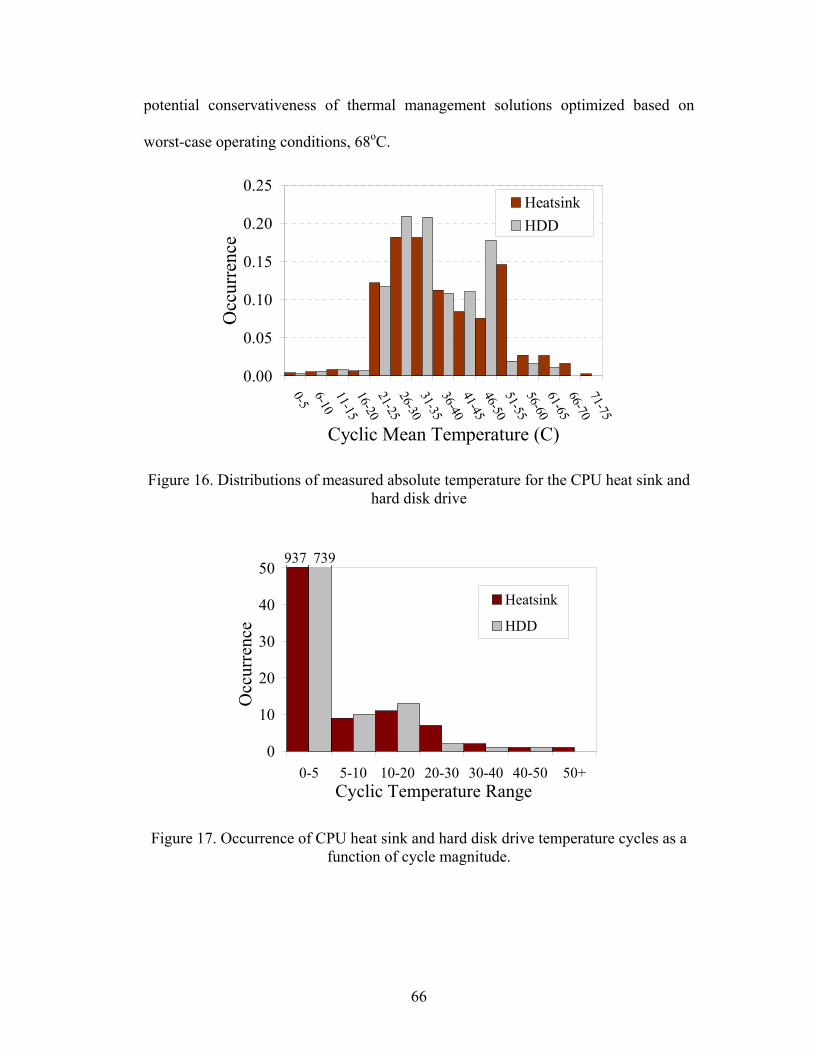
66
potential conservativeness of thermal management solutions optimized based on
worst-case operating conditions, 68oC.
0.00
0.05
0.10
0.15
0.20
0.25
0-56-1011-1516-2021-2526-3031-3536-4041-4546-5051-5556-6061-6566-7071-75
Cyclic Mean Temperature (C)
Occ
urre
nce
HeatsinkHDD
Figure 16. Distributions of measured absolute temperature for the CPU heat sink and hard disk drive
0
10
20
30
40
50
0-5 5-10 10-20 20-30 30-40 40-50 50+Cyclic Temperature Range
Occ
urre
nce
Heatsink
HDD
937 739
Figure 17. Occurrence of CPU heat sink and hard disk drive temperature cycles as a function of cycle magnitude.

67
0.00
0.05
0.10
0.15
0.20
0.25
0.30
0.35
R<11<R<2
2<R<44<R<6
6<R<88<R<10
10<R
Ramp-rate (degree C/min)
Occ
urre
nce
HeatsinkHDD
Figure 18. Distribution of measured temperature cycle ramp rates for the CPU heat sink and hard disk drive. R refers to temperature cycle ramp rate
Figure 17 indicates that about 97% of the temperature cycles experienced by
either the CPU heat sink or HDD have amplitude of less than 5oC. In addition, the
CPU heat sink experiences about 25% more such cycles than the HDD. While it is
generally perceived that temperature cycles of small amplitude may not significantly
impact on the reliability of electronic packaging interconnections, the potential
damage induced also depends on variables such as the mean cyclic temperature, ramp
rate, and dwell temperature, as highlighted by [118], [119] for solder joint fatigue.
Pump-out of the thermally-conductive grease at CPU-heat sink interfaces, which lead
to increased interface thermal resistance, has been attributed to temperature cycling
having an amplitude comparable to those measured in this study, around 5oC [120].
The monitored temperature data therefore suggests that the effect of such multiple
mini-cycles on interconnection reliability should be further investigated for the range
of measured mean cyclic temperatures and ramp rates. This highlights the
importance of recording such data. On the other extreme, temperature cycle

68
magnitudes of up to 50oC were also measured (see Figure 17). This exceeds the
worst-case use condition specified by standard IPC SM-785 [71] for consumer and
computer products, namely 30oC and 20oC respectively. Such a discrepancy between
standardized and actual conditions provides a strong motivation for monitoring actual
product application environments.
The measured temperature ramp rate distribution shown in Figure 18 would
also permit more accurate predictions of solder joint fatigue life to be obtained than
using worst-case ramp rate specifications [71]. For example, Figure 18 shows that
over 80% of the total time period, the temperature cycles experienced by the CPU
heat sink have a ramp rate of less that 4oC/min, while temperature ramp rates
exceeding 10oC/min are observed over less than 3% of the total time.
Monitored life cycle temperature data, such as presented in Figure 16 to 18,
could be applied in a life consumption monitoring methodology, to provide both
damage estimation and remaining life prediction due to specific failure mechanisms
influenced by temperature. For example, measured heat sink base temperature data
could be used to assess the reliability of component-to-heat sink adhesive
attachments. Examples include [72], [73], [74] and [75], which evaluated the impact
of differential thermal expansion and creep-induced degradation on component-heat
sink adhesive joints, respectively. The measured data could also be used to determine
the stress levels to be imposed in accelerated testing, refining product specifications,
and setting product warranties.

69
While a comprehensive health monitoring process would involve other
environmental variables, such as humidity, vibration and shock, apart from
temperature, a line of approach similar to that presented in this study could be applied
to monitor such life cycle loads. Similarly, the proposed approach could be extended
to other electronic products. A list of variables (not exhaustive) for monitoring the
entire laptop is proposed in Table 6.
Table 6. Environmental, usage and performance parameters for PHM of notebook computers
Parameters Examples
Environmental
and Usage
- Temperatures of microprocessor, hard disk drive, video card,
RAM etc.
- Vibrations/shock in application and handling, disk spin
- Processor usage, memory usage, processor queue length, Cache
fast reads/second etc.
- Power cycles, number of on/off
- Hard disk and monitor on/off
- Strain in mother board flexing and torsion during handling and
due to ageing
- Pressure on keyboard and buttons
- Force on latch, hinge, and connectors
- Humidity and radiation exposure
Performance
and system
setup
- Fan ON/OFF, Fan speed
- CPU core voltage, CPU I/O voltage
- Hard disk parameters: spin-up time, flying head height, ECC
count, data transfer rate
- Power management settings (power schemes, hibernate, and
stand-by settings)

70
4.3 Conclusions
A method of environmental, operational and usage data collection for
enabling health monitoring of electronic products was presented. To implement this
methodology in a real system, guidelines were provided on the selection of
monitoring parameters and the design of a monitoring plan. An integrated hardware-
software module was suggested for in-situ monitoring and processing of load data in
the life cycle environment. The main attributes for selecting the sensor system for
these applications were identified to be the level of integration, power consumption
and management, on-board memory and utilization, low size and weight, wireless
communication, embedded computational power, and software support. Methods to
improve the efficiency of the data collection process by reducing power consumption,
by making effective use of memory, and by integrating embedded computational
power with sensor systems were discussed. Using field data the trade-off between
data reduction and error in damage accumulation was demonstrated. The analysis
showed that more than ninety percent data reduction only accounted for less than one
percent error in damage accumulation.
The thermal loads in a notebook computer were dynamically monitored in-situ
for typical usage, transportation and storage environments, and statistically analyzed.
The effects of power cycles, usage history, CPU computing resources usage and
external thermal environment on internal peak transient thermal loads were
characterized.

71
The CPU heat sink temperature was found to be 13oC and 8oC lower than its
maximum rating over 90% and 95% of the monitored time period, respectively. This
highlights the potential conservativeness of thermal management solutions optimized
based on worst-case operating conditions that rarely occur. Such findings could
contribute to the design of more sustainable, least-energy consumption thermal
management solutions.
About 97% of the temperature cycles experienced by either the CPU heat sink
or HDD had amplitude of less than 5oC. However, the maximum temperature cycle
amplitudes measured were found to exceed those specified by environmental
standards for computer and consumer equipment. This provides a strong motivation
for monitoring actual product application environments.
72
Chapter 5: Methodology for Extracting Load Parameters from Time-Load Signals
5.0 Introduction
This paper presents a novel method for processing the in-situ monitored load
data to enable prognostic assessment of electronic products and systems. The
proposed method processes the time-domain sensor data to extract load parameters
including cyclic ranges, mean load, ramp-rates, and dwell times. The load parameters
and their correlations are then used in conjunction with damage models for assessing
and predicting the health due to commonly observed failure mechanisms in
electronics. An algorithm was developed that enables significant reduction of large
irregular time-load data without compromising load parameters essential for damage
estimation and enables compact storage of load histories. The approach was
demonstrated using a case-study of an electronic board subjected to irregular
temperature cycles. The methodology can be used for processing other load signals in
time domain including strain, humidity, voltage etc.
5.1 Review of Existing Load Parameter Extraction Methods
Several methods have been developed and reported that can extract
parameters from time-load data [76-86]. Currently available methods are briefly
discussed in Table 7. A cycle is defined when the time-load signal crosses it previous

73
peak or valley before changing its direction. In Figure 19 b-c-b’ is a complete cycle,
while a-b-d is a half cycle.
Figure 19. Geometric definition of a cycle
Table 7. Review of existing load parameter extraction methods Load Extraction
Method
Description
Hayes Method Hayes’ method identifies small ranges, which are interruptions of
a larger range. An interruption is found for a peak-valley pair
when the next peak is higher than the current peak. An
interruption is found for a valley-peak pair when the next valley is
lower than the current valley. Once damage is calculated for these
cycles, they are screened out of the original block of data,
producing the abbreviated blocks. The procedure is repeated to
cover all blocks.
Ordered Overall
Range
The OOR method (also called the Racetrack method) converts
irregular data in sequence of peaks and valleys. The sequence of
reversals in the original profile into a racetrack by offsetting the
profile by a selected track width or screening level (S). Peaks and
valleys that were originally separated by smaller interrupting
ranges now become adjacent, creating larger overall ranges.
Level Crossing In this method a count is recorded whenever an increasing
Cyclic range
Cyclic mean
Time
Load
a
b
c
d
Full cycle
half cycle
b’Cyclic range
Cyclic mean
Time
Load
a
b
c
d
Full cycle
half cycle
b’

74
Counting (positively sloped) portions of the load history crosses a certain
level above the reference level. Likewise, a count is recorded
when a decreasing (negatively sloped) portion of the load history
crosses a certain level above the reference level. Cycles are
constructed by counting in an order to form most damaging
reversals.
Peak Counting Peak counting records relative maxima and minima in the load
history and their load levels. Generally only peaks and valleys
above and below set reference levels are counted. Similar to level
crossing the most damaging cycle is recorded between the largest
peak and valley.
Simple-Range
Counting
Simple range refers to the difference in the load levels of the
successive reversals. Both positive and negative slopes can be
counted. The method can be non-conservative and miss an overall
large cycle.
Range-Pair
Counting
In range pair counting, two subsequent ranges of opposite sign are
considered together. If the second range is greater than or equal to
the first range in size, the first range is counted, and the peak and
valley are removed from consideration. If the second range is
smaller then the next range is considered, and so on.
Rainflow
Counting
In Rainflow counting two consecutive ranges are considered
together. Based on a set of rules the algorithm scans the entire
time-load history to identify full cycle and half cycles. The
Rainflow method provides the mean stress in addition to the
stress range during counting.
5.2 Limitations of Existing Methods
The limitations with existing load extraction methods for application in
electronic prognostics and health assessment include (1) inability to extract ramp

75
rates and dwell time, (2) need for smart data reduction and filtering techniques, and
(3) need for assessing correlation of load parameters, are discussed below.
5.2.1 Extracting ramp rates and dwell information
The existing load extraction methods provide the load range and mean load.
These parameters can be adequate parameters for fatigue life estimation in elastic-
plastic fatigue analysis of materials. However, for example, in case of thermal-fatigue
loads (frequently observed in electronic systems), wherein the damage is
characterized by plastic yielding and creep deformations, the estimation of dwell time
and ramp rates is required in addition to the stress range and mean stress for accurate
fatigue assessment. Ramp rates can be estimated with modifications in the Rainflow
algorithm. However, extracting dwell times and corresponding load levels is more
challenging since it depends on both the amplitude and ramp rate of the monitored
load cycles.
Along with electronic applications, dwell times are also crucial in estimating
fatigue life of other components. For examples of fan disk failures have been reported
due to dwell sensitivity [87]. Hold periods of few minutes to several hours are applied
in gas turbines [87], [88] and for weeks or more for power plant components that
affect the remaining life of components. Other examples of applications were
components are affected by creep-fatigue data are; electronic packaging, space shuttle
nozzle liners, power plant components, gas turbine nozzles [89], furnace tubes [90].

76
Various materials that have been studied and have shown dwell sensitivity:
solder alloys (96.5% Pb-3.5% Sn) and other solders commonly used in PCB
assembly, copper alloy (NARloy and AMZIRC), low alloy steels (1-Cr-Mo-V, 1.25
Cr – Mo, and 2.25Cr-Mo), stainless steel (SS 316), titanium alloys (IMI 318 and IMI
829), and super-alloys (MAR M 002, waspaloy, Rene 95, Rene 90, inconel 617, In
100, PWA 1480 and MA 754) [91], [92].
5.2.2 Concerns with data reduction
Analysis of complex load histories typically involves a data reduction stage to
enable efficient data processing and eliminating undesired load reversals. However,
data reduction methods can eliminate important load information and avoid the
extraction of certain loading parameters in subsequent stages. For example the
Ordered Overall Range (OOR) can eliminate small cycles (as a fraction of large
cycles) by choosing an appropriate value of S-parameter (S < 1). However, in the
process it also deletes the dwell-time information. In Figure 20, the points and lines
in light shade depict the original data before reduction. The dark line connecting the
end points depicts the results obtained after OOR. The load information of 0.2 hours
of dwell time at 60oC is important for assessing damage due to creep mechanisms at
various locations on the electronic assembly such as solder joints, plated through
holes, and die-attaches.

77
Figure 20. Data reduction methods can potentially eliminate dwell regions
5.2.3 Correlation of load parameters
Distributions of in-situ monitored temperature load parameters can be
randomly sampled and used with the damage model in a Monte Carlo simulation. For
accurate damage assessment the correlation between load parameters is important.
Quantifying and using the correlations for damage assessment, enables generating
realistic scenarios during random sampling. For example, the distributions of
measured ∆T and Tmean can be used for assessing the solder joint damage due to
cyclic thermal loading. However, it is essential to know the correlation between these
two parameters, as cycles with small ∆T but higher Tmean values will cause more
damage than the cycles with same ∆T values but lower Tmean.
5.3 Methodology for Load Extraction
An algorithm was developed to process a given a time (t) versus temperature
(T) signal, to extract cyclic range ∆T, cyclic mean temperatures (Tmean), ramp rate
(dT/dt) , dwell time tD and temperature of dwell. Additionally, the correlation
20
25
30
35
40
45
50
55
60
65
0 0.1 0.2 0.3 0.4 0.5 0.6 0.7 0.8 0.9 120
25
30
35
40
45
50
55
60
65
0 0.1 0.2 0.3 0.4 0.5 0.6 0.7 0.8 0.9 1
Time (hours)
Tem
pera
ture
(o C)

78
between, dwell times versus temperature of dwell, cyclic range versus mean
temperatures, and cyclic range versus ramp rates are quantified in terms of correlation
coefficient. These load parameters can then be used in conjunction with damage
models in Table 4 to assess the damage at various failure sites due to different failure
mechanisms for a given electronic assembly. The entire process is implemented in a
software program, which contains the details of the electronic board and component
material properties and geometries, to enable rapid assessment.
The algorithm starts by processing the irregular time-load data using a moving
average filter to remove the noise.
In the above equation ‘a’ is the smoothening parameter. For the moving
average to reduce the random noise while retaining the sharp response, the value of
smoothening parameter ‘a’ is selected as the nearest integer of the square root of
sampling frequency in Hz.
Typically a filter with a smoothing factor derived from above equation has
been reported to provide adequate noise reduction for various signal types without
changing the original signal (Figure 21).
In the next step small ranges are merged into overall increasing, decreasing, or
dwell data streams. A range threshold value is selected to merge small ranges. All
∑−+
=)1(
)(1)('an
nts
ats
( )fhzINTa =

79
ranges in the given data set that are less than delta s are merged in the larger overall
range. An optimal range threshold value enables efficient load data reduction method,
permits gains in computing speed, condenses load histories without sacrificing
important damage characteristics and preserves the most damaging reversals in the
original loading
Figure 21. Results of MA filter with different smoothening parameter based sampling frequency
Range threshold value is based on the significance of the range in the damage
model. For e.g., If, Damage α (∆T)n , then for all n > 1, threshold range can be
selected as the nth root of the maximum ∆T measured i.e., = (∆Tmax/2)^(1/n). For
damage models with n between 0 and 1, the threshold range value =
(∆Tmax/2)^(0.75) can eliminate small cycles without introducing significant errors in
the damage estimations (Figure 22).

80
Figure 22. Threshold level increases as value of power in damage law (n) decreases
In case of measured field data it can be challenging to identify dwell
temperature regions. This is because dwell regions may appear as a series of small
cycles with a constant or near constant mean (Figure 23c), or it can also appear as a
relatively large cycle with an extremely slow ramp rate (Figure 23c). For example, if
the range threshold is ∆T less than 5oC, then several consecutive cycles with ∆T< 5oC
is considered dwell. However, a cycle with say, ∆T = 10oC but a slower ramp-rate is
also considered as dwell. Based on these criteria, the algorithm scans the time-
temperature data and identifies the dwell temperatures and dwell times.
The correlation coefficient between dwell time and dwell temperatures is
calculated and stored. The actual values of dwell time and dwell temperatures are
then stored in a histogram with optimal bin-widths. The bin-data is used with kernel
functions to estimate the probability density of the measured values. This method
enables enormous on-board storage reduction and improves the ability of the sensor
module to monitor for longer time durations. The significance of optimal binning and
density estimation will be discussed in section 5.6.
05
10152025303540
0 50 100 150 200 250Maximum Delta T
Thre
shol
d va
lue
(del
ta T
)
n = 1n = 1.5n = 2n = 4

81
The time-temperature data is then scanned for identifying full cycles. The
geometric definitions of full and half cycle are well documented [80]. The time-
temperature data is scanned to identify if ∆Ti is a full cycle based on the condition
∆Ti-1 > ∆Ti ≤ ∆Ti+1 (Figure 23d). For each cycle the mean temperature and ramp-rate
is recorded. The full cycle is then removed from the stream and the residual time-
temperature containing half cycles is data is merged with original time stamp being
retained. The process is iterated till all full cycles are identified and stored in the
appending matrix. The remaining half cycles are then converted into full cycles. At
the end of cycle counting the correlations between temperature range versus mean
temperatures, and temperature range versus ramp rate are assessed and recorded. The
load parameter values are then stored in histogram with optimal bins as described
previously. The entire procedure for load parameter extraction is shown in Appendix
I. The on-board memory is cleared by deleting the matrix containing the load
parameters and only the histograms and correlation values are retained.

82
Figure 23. (a) Reduces noise using moving average filter (b) Eliminates monotonic data patterns and merges small ranges into overall data streams (c) Identifies dwells
temperatures and time using ramp-rate and range (d) Scans the time-temperature data to extract cyclic load parameters
5.4 Demonstration
The proposed load parameter extraction method was first tested using simple
data sets. Various time-temperature data series were generated to evaluate the ability
of the algorithm to correctly identify dwell regions based on small cycles and ramp-
rates. For the cycle counting part, the algorithm is primarily based on the proven and
tested Rainflow cycle counting method, and hence additional rigorous testing was not
required.
Sensor data
MA filtert
∆T
t
∆Ts
t0
20
1
2
3
4
5
6
7
8
9
10
11
12
13
14
15
16
17
18
19
0
20
1
2
3
4
5
6
7
8
9
10
11
12
13
14
15
16
17
18
19
t
T
Time (seconds)
Tem
pera
ture
(o C)
(a)
(b)
(c)(d)
Sensor data
MA filtert
∆T
tt
∆Ts
t0
20
1
2
3
4
5
6
7
8
9
10
11
12
13
14
15
16
17
18
19
0
20
1
2
3
4
5
6
7
8
9
10
11
12
13
14
15
16
17
18
19
t
T
0
20
1
2
3
4
5
6
7
8
9
10
11
12
13
14
15
16
17
18
19
0
20
1
2
3
4
5
6
7
8
9
10
11
12
13
14
15
16
17
18
19
t
T
Time (seconds)
Tem
pera
ture
(o C)
(a)
(b)
(c)(d)

83
The application of the proposed method was then demonstrated for electronic
prognostics by processing in-situ monitored temperature data. An electronic assembly
was exposed to irregular temperature cycles using a programmable oven to simulate
field conditions. The irregular profile was generated produce temperature cycles with
a different ranges, means, ramp-rates, and dwell times. Temperature extremes ranged
from -50oC to 160oC and dwell times were randomly selected as multiples of five
between 0 to 30 minutes. Also long dwell times were recorded at room temperatures
when the oven was shut-down to simulate non-operating conditions. A snapshot of 20
days of temperature exposure out of 110 days is shown in Figure 7.
The time-temperature data was processed using the steps shown in Figure 23
and Appendix-I that were implemented in a visual basic for applications environment.
The resulting distribution of cyclic temperature ranges, means, ramp rates, and dwell
times is shown in Figure 22-25. The histogram of dwell times shows that the
algorithm correctly identified the dwell regions that were programmed between 0 to
30 minutes (Figure 26). Also, the longer temperature dwell periods (> 160 minutes)
programmed to represent the non-operating periods were correctly identified.
The correlation between the load parameters is shown in Figure 26-28. From
Figure 27 shows that the occurrence of the longer temperature dwell corresponds to
temperatures in the range of 25-27oC. The correlation coefficients (ρ) of -0.84 shows
an inverse correlation, i.e., a low value from dwell time distribution corresponds to
high value in dwell temperature distribution and vice versa. The use of these
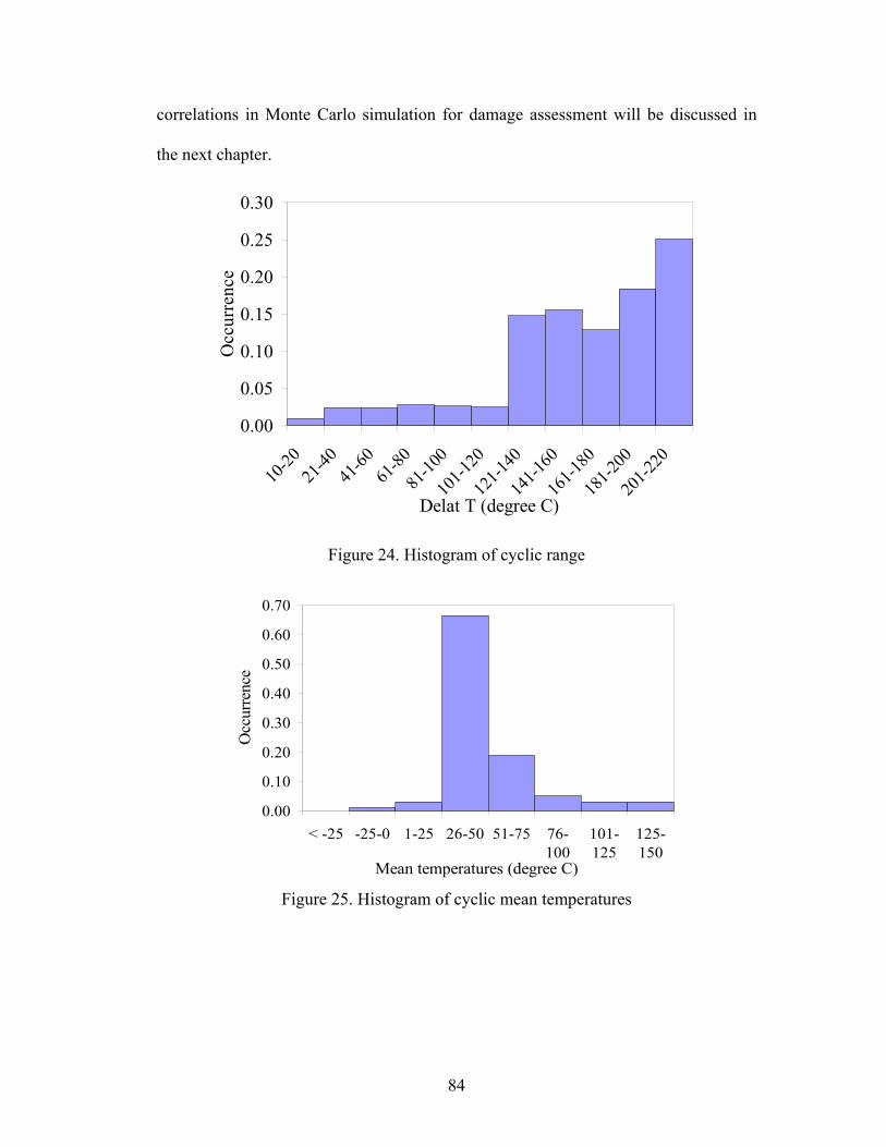
84
correlations in Monte Carlo simulation for damage assessment will be discussed in
the next chapter.
0.00
0.05
0.10
0.15
0.20
0.25
0.30
10-20
21-40
41-60
61-80
81-10
0
101-1
20
121-1
40
141-1
60
161-1
80
181-2
00
201-2
20
Delat T (degree C)
Occ
urre
nce
Figure 24. Histogram of cyclic range
0.00
0.10
0.20
0.30
0.40
0.50
0.60
0.70
< -25 -25-0 1-25 26-50 51-75 76-100
101-125
125-150
Mean temperatures (degree C)
Occ
urre
nce
Figure 25. Histogram of cyclic mean temperatures

85
0.00
0.10
0.20
0.30
0.40
0.50
0.60
0.70
0-0.5 0.51-1.0
1.01-1.5
1.51-2.0
2.01-2.5
2.51-3.0
3.01-3.5
Ramp-rate (degree C/min)
Occ
urre
nce
Figure 26. Histogram of ramp-rates
0.00
0.10
0.20
0.30
0.40
0.50
0.60
0-10 10-20 20-40 40-80 80-160 160-320Dwell time (minutes)
Occ
urre
nce
Figure 27. Histogram of temperature dwell times

86
Figure 28. Correlation between dwell time and temperature
Figure 29. Correlation between delta T and mean temperatures
Figure 30. Correlation between delta T and ramp-rate
0
25
50
75
100
125
150
0 50 100 150 200 250 300 350
Tem
pera
ture
(o C)
Dwell time (mins)
0
25
50
75
100
125
150
0 50 100 150 200 250 300 350
Tem
pera
ture
(o C)
Dwell time (mins)
0.0
0.5
1.0
1.5
2.0
2.5
0 50 100 150 200 250Delta T (oC)
Ram
p ra
te (o C
/min
)
0.0
0.5
1.0
1.5
2.0
2.5
0 50 100 150 200 250Delta T (oC)
Ram
p ra
te (o C
/min
)
-60
-20
20
60
100
140
0 50 100 150 200 250
T mea
n(o C
)
Delta T (oC)
-60
-20
20
60
100
140
0 50 100 150 200 250
T mea
n(o C
)
Delta T (oC)

87
5.5 Method for Binning and Density Estimation
The extracted load parameters are stored in appropriate bins to achieve further
data reduction. The binned data is downloaded to estimate the distributions of the
load parameters for use in damage assessment, remaining life estimation, and the
accumulation of the products use history. Since the accuracy of the damage
assessment and remaining life prognostics depend on the accurate estimate of the
probability density functions (pdf) of the loads derived from the binned data, it is
essential to select the appropriate bin-width and number of bins a-priori.
This paper provides a method for applying optimal binning techniques for
enabling condensed storage of in-situ monitored load histories. Optimal bin-widths
relations are used in conjunction with non-parametric density estimation techniques,
namely the histograms and kernels. The approach is then demonstrated.
5.5.1 Optimal Binning and Density Estimation
If the entire data set, without data binning, is retained, a parametric method
can be used for density estimation. In that case the objective is to find a best fitting
parametric function to the given data. Standard parametric functions include normal,
lognormal, exponential, and Weibull, described by parameters such as mean and
standard deviation. If the underlying distribution is non-standard (e.g., multi-modal),
fitting a single standard parametric function to the data can result in errors, and fitting
multiple parametric functions can make the problem solution non-unique. Non-
parametric methods can be used to estimate the pdf without assuming any parametric

88
structure [93], [94]. Examples of non-parametric density estimation methods include
histograms, Kernels, orthogonal series estimation, and nearest neighbor method. In
our study, histograms and kernel estimators were used.
Histograms
A histogram is a graphical representation of a frequency distribution in which
the height of the bins represents the observed frequencies. The choice of bin-width
primarily controls the representation of the actual data. Smaller bin-widths may
present too much details (undersmoothing) and larger bin-widths may present or too
less details (oversmoothing), of the true distribution [93]. Histograms are based on an
equally spaced bin-width hn where n denotes the sample size. If is the estimate
of the true density f(x), then the global accuracy of the estimate can be evaluated by
the integrated mean square error that is defined by.
(1)
The IMSE is the sum of the integrated square bias and integrated variance, the
bias being the difference between the true density and the estimate. The bin-width
that minimizes the IMSE is required for accurate estimation of the true pdf f(x). Scott,
[95], derived the asymptotically optimal choice of bin width, hn* as;
(2)
Since hn* depends on the unknown pdf f(x), an estimate of f(x) can be
plugged into equation 2. For the normal distribution, the approximate optimal bin-
width is;
(3)
)(ˆ xf
[ ] dxxfxfEIMSE2
)()(ˆ −= ∫
3/13/1
23/1* )('6 −−∞
∞− ⎟⎟⎟
⎠
⎞
⎜⎜⎜
⎝
⎛
⎟⎟
⎠
⎞
⎜⎜
⎝
⎛= ∫ ndxxfhn
)(ˆ xf
3/1* 49.3 −= snhn

89
where s is the sample standard deviation and n is the sample size. Freedman
and Diaconis [96] suggested another bin width formula that can be applied to non-
Gaussian data;
(4)
where IQR is the inter-quartile range of the data (Q3-Q1). Several other
studies have focused on more quantitative and qualitative aspects of bin width
selection [96]–[100]. Once the bin width is calculated, the histogram is defined as;
nhxf 1)(ˆ = (number of Xi in the same bin as x) (5)
Kernel Estimators
Kernel density estimators [101] are non-parametric methods used to estimate
f(x) using the kernel estimator K (also called a window function) defined as;
(6)
where h is the bin width, also called as smoothing parameter or band width.
Equation 6 can be considered as a pdf obtained by averaging the effect of a set of
local functions K centered at each data point x. A variety of kernel functions with
different mathematical properties have been reported [102]-[106]. Commonly used
kernel functions include uniform, Gaussian, triangle, Epanechnikov, and biweight.
Kernel functions are generally chosen based on the ease of computation and desired
properties of the function. For example, the Gaussian kernel is used for its continuity
and differentiability. The optimal bin width for the Gaussian kernel (equation 7) is
obtained by minimizing the integrated mean square error (equation 8).
3/1* )(2 −= nIQRhn
∑=
⎟⎟⎠
⎞⎜⎜⎝
⎛ −=
n
j
jh h
xxK
nhxf
1
1)(ˆ

90
(7)
(8)
where s is the estimate of standard deviation. The Gaussian kernel can be
used for non-Gaussian data, since the kernel is used only as a local weighting
function [94].
5.5.2 Implementation Approach for PHM
For in-situ monitoring over long durations, one can use the load measurements
obtained in the past or the data monitored over initial few periods to obtain the
estimate of sample size and standard deviation. The relations provided in equation (3)
and (7) are then used for bin width calculations. Once the bin-widths are calculated,
the data for the subsequent time periods is stored directly in the bins. At the end of the
monitoring period, the bin-widths and frequency is used in conjunction with
equations (5) and (6) to obtain the probability distributions. These distributions are
then used for damage assessment and prognostics (see Figure 31).
The load parameters obtained during monitoring depend on the usage and
environmental conditions during the monitoring period. Thus, depending on usage
conditions, there could be differences between the estimated and actual values of
sample size and standard deviation. These differences can lead to inaccuracies in the
subsequent density estimation process. One approach to overcome this problem is by
recording the actual values of standard deviation and sample size during monitoring
5/1ˆ06.1 −= nshopt
2/22/1)2()( xexK −−= π

91
and using these values for density estimation. One can update the value of standard
deviation every time a data point is added to the bins and also keep a track on the
sample size. The advantage of continuously updating the standard deviation is that it
does not require storing the complete data set. Optimal bin-widths can then be
recalculated based on actual values of sample size and standard deviation to estimate
the probability distribution (see Figure 31).
Figure 31. Approach for binning and density estimation of monitored load parameters
5.5.3 Results
The rest of the discussion will focus only on binning and density estimation of
cyclic Tmean, values extracted using methods discussed in section 5.3. The same
procedure used for binning and density estimation of all other load parameters. For
the first five days of the experiment, the cyclic Tmean data was extracted and stored
without any binning. The average samples size (n), standard deviation (s), and inter-
quartile range (IQR) for each load parameter was then calculated (see Table 8). These
values were used as estimates of s, n, and IQR in equations (3), (4), and (7) to
calculate the optimal bin widths for both histograms and kernels. For the histograms,
Calculate optimal bin width based on estimate of standard deviation and
sample size from historic sensor data
Monitor and store load parameter in bins based on optimal bin width
Estimate density based on bin-widths and frequencies with Gaussian kernel
Calculate optimal bin width based on estimate of standard deviation and
sample size from historic sensor data
Monitor and store load parameter in bins based on optimal bin width
Estimate density based on bin-widths and frequencies with Gaussian kernel

92
the optimal bin widths obtained from equations (3) and (4) were within +/- 5%. This
is in agreement with results reported in the literature [96].
After the fifth day, the load parameters were extracted and stored in the bins
calculated from the five day estimate. The bin frequencies were downloaded and
distributions of load parameters were derived using histograms (see equation 5) and
kernel functions (see equation 6). The percentage of data reduction due to use of the
bins was measured. The ability of histograms and kernel functions (using binned
data) to represent the complete data set was assessed by comparing the histograms
and kernel plots with the parametric distributions that were best fitted to the complete
data set.
Table 8. Estimate of parameters used for the bin width calculation
Day Sample size
(n)
Inter-quartile
range (IQR)
Standard
deviation (s)
1 97 110.77 59.10
2 80 131.20 66.70
3 72 101.81 60.94
4 80 36.63 48.89
5 90 135.96 68.68
Average 84 103.27 60.68
The best fitting distribution for the complete data set of Tmean values obtained
on day 6 was found to be a normal distribution (see Figure 32). The distribution
obtained using histogram (equation 5), based on data binned as per equation 3, is
shown in Figure 32. The solid dark line in the Figure 32 shows the distribution of

93
Tmean values obtained from binned data and using the Gaussian kernel. It is observed
that the true shape of the distribution obtained from the data is bi-modal, which is
accurately represented by the kernel and histogram. This bi-modal nature of Tmean
values was hidden by the smooth normal distribution.
When the distributions were used in the Monte Carlo simulation model for
damage assessment, the samples of Tmean values drawn from the kernel resulted in
more accurate estimates of damage, since the samples were drawn from a distribution
that accurately represented the measured data. In comparison to the histogram, the
kernel density estimate is smoother. Hence during random sampling, more number of
distinct samples were drawn from the kernel distribution as compared to the
histogram. This further improved the accuracy of the damage distribution resulting
from the Monte Carlo.
In terms of data reduction, the use of kernels and histograms resulted in 78%
and 85% less data per day compared to using the complete monitored data set.
Assuming the same amount of data reduction, the sensor system with binning can
now be used uninterrupted for 6.6 more days with histogram and 4.7 more day with
kernels to consume the same storage space without binning. Similar results were
obtained when the analysis was conducted from day seven onwards. This clearly
demonstrates the importance of these methods to enable uninterrupted monitoring at
low power and memory consumption.

94
Figure 32. Comparison of density estimates for Tmean values of day 6
The sensitivity of the kernel densities to the difference between estimated and
actual standard deviation and sample size were investigated by analyzing the
experimental data for different time periods. For example, Figure 33 compares three
density estimates estimated using Gaussian kernel; distribution (1) is obtained using
the complete data set and actual values of standard deviation and sample size for
calculating is hopt. Distribution (2) is based on binned data and estimated values
standard deviation and sample size for calculating is hopt. Distribution (3) is obtained
from binned data and updated values standard deviation and sample size using the
approach in Figure 31. In this example, the difference between the actual and
estimated s was 38%. It is observed that the distribution (3) using updated value is a
better estimate of the actual distribution (1). Similar results were obtained for

95
different sets of data collected in the study. More information is available in a paper
on this work by the author [107].
Figure 33. Comparison of distributions obtained from estimated versus actual parameters
5.6 Conclusions
A novel method was developed for extracting cyclic range, mean, ramp rates,
dwell times and their correlations, from irregular time-temperature history. The
application of this method for electronic prognostics and health management was
demonstrated. The method for parameter extraction combined with storage of load
parameters in bins resulted in 99.03% storage reduction per day, without
compromising dwells regions. Thus embedding this algorithm with the sensor module
can significantly enhance the ability of the module to monitor for longer durations

96
without running out of memory. The method can also be used for processing different
time-load signals such as strain, acceleration, and humidity.
For prognostics and health management, the application of optimal binning
and density estimation using histogram and kernel estimators for condensed storage
of load histories, can significantly improve the ability of the sensor nodes to monitor
for extended durations without interruptions and conserve memory and power. It was
found that optimal bin widths can be calculated a-priori based on estimates of sample
size and standard deviation of representative data sets. In using the binned data for
representing the entire data set, kernel methods provided a better estimate of the
probability density compared to histograms. It was shown that the difference between
the estimated and actual bin-width and the resulting error in density estimation can be
minimized by recording the sample size and standard deviation during in-situ
monitoring, and using the recorded (true) values for density estimation.

97
Chapter 6: Prognostics Approach Considering Uncertainties
6.0 Introduction
The ability to predict a product’s remaining life with the associated
confidence limits, based on current and historic “health” conditions can enable
effective maintenance and reduce the life cycle cost by decreasing inspection,
downtime, and inventory costs. Remaining life predictions are made by assessing the
accumulated damage due to measured environmental and usage exposure. However,
often the effect of uncertainty and variability in the measurement and procedures used
for making predictions is neglected. In this chapter, a generic method is developed
for remaining life prognostics that accounts for the measurement, model-input, and
model uncertainties. The method is demonstrated to predict the remaining life
distributions of solder interconnects subjected to field temperature conditions. The
details of the proposed method and the implementation case-study are presented.
6.1 Background
For electronics prognostics, a method to predict remaining life using life cycle
loads was proposed by Ramkrishnan and Pecht 2003 [53], referred as life
consumption monitoring (LCM). LCM methodology is a six-step process, (see
Figure 34), that combines systematic study of the different failure modes and
mechanisms of the product under consideration, monitoring of relevant environmental
and/or operational parameters, and use of physics of failure models to asses the
damage and ultimately predict remaining life. For demonstration of this approach to

98
electronic assembly, Mishra et al. 2002 [54] and Ramakrishnan and Pecht, 2003 [53]
monitored the temperature, humidity, vibration and shock loads experienced by an
electronic assembly operated in automotive under-hood environments. This
monitored data was applied in conjunction with physics-of-failure models to estimate
damage and predict remaining life. The PHM methodology was shown to accurately
predict remaining life in the application environment.
Figure 34. CALCE Life consumption monitoring methodology
One of the major drawbacks of this approach was the use of discrete values of
loads for making damage assessments, which results in discrete values of damage
fractions and remaining life. This approach did not consider the various uncertainties
and variability that can significantly influence the prognostics. These uncertainties
include i) measurement uncertainty, due to inaccuracies in the sensing, recording, use
Step 1: Conduct failure modes, mechanisms and effect analysisStep 1: Conduct failure modes, mechanisms and effect analysis
Step 6: Estimate the remaining life of the productStep 6: Estimate the remaining life of the product
Step 5: Perform physics-of-failure stress and damage accumulation analysisStep 5: Perform physics-of-failure stress and damage accumulation analysis
Continue monitoringContinue
monitoring
Is the remaining-life
acceptable?
No
Yes
Step 4: Conduct data simplification to make sensor data compatible with physics-of-failure model requirements
Step 4: Conduct data simplification to make sensor data compatible with physics-of-failure model requirements
Schedule a maintenance actionSchedule a maintenance action
Step 3: Monitor appropriate product parameters such as environmental (e.g, shock, vibration, temperature, humidity)
operational (e.g., voltage, power, heat dissipation)
Step 3: Monitor appropriate product parameters such as environmental (e.g, shock, vibration, temperature, humidity)
operational (e.g., voltage, power, heat dissipation)
Step 2: Conduct a virtual reliability assessment to assess the failure mechanisms with earliest time-to-failure
Step 2: Conduct a virtual reliability assessment to assess the failure mechanisms with earliest time-to-failure

99
of sampled information, and assumptions in data conditioning techniques. ii)
Parameter uncertainty, which arises due to variability in the material and geometric
parameters that are used in the damage model for health evaluations. iii) Model
uncertainty, which may arise due to limitations in analyst’s knowledge of
phenomenon and deliberate simplifications introduced for modeling.
The essence of prognostics is the estimation of remaining life in terms that
have consequence in the maintenance decisions process [108]. Using the life
consumption monitoring approach with single point estimates of remaining life,
without confidence intervals and confidence level, it may not be possible to take
logistics decisions with certainty. Hence it is necessary to identify the uncertainties in
the prognostic approach and assess the impact of these uncertainties on the remaining
life distribution, in order to make risk-informed decisions.
In this work we have developed an approach to account for the measurement,
parameter, and model uncertainties in the prognostics process. The approach
combines sensitivity analysis and Monte Carlo based random sampling to provide a
distribution of accumulated damage. Using regression analysis of the accumulated
damage distributions, the remaining life is then predicted with confidence intervals
and levels. The approach is demonstrated using a PHM setup discussed in chapter 3.
6.2 Overview of Methodology
A generic approach was developed for making predictions by considering the
measurement, parameter, and model uncertainty. Figure 35 presents the schematic of

100
the approach adopted in this work for estimating the confidence bounds on the
remaining life predictions. The next few sections will discuss in detail on the building
blocks of the approach.
6.2.1 Measurement Uncertainty
Environmental and usage load profiles are captured in the application
environment, for utilizing in real time or near real time health assessment and
prognostics using sensors and data loggers. This raw sensor data is simplified or pre-
processed to make it compatible with the damage models and algorithms that are used
to conduct prognostics. In particular, it may be necessary to extract the relevant load
parameters including cyclic mean, amplitudes, ramp rates, hold periods, power
spectral densities, etc. Commonly used load parameter extraction methods include:
cycle counting algorithms for extracting cycles from time-load signal, Fast Fourier
transforms (FFT) for extracting the frequency content of signals, etc. Depending on
the application and type of signal, custom load extraction methods may be required.
Figure 5 (chapter 3), provides a schematic of the in-situ monitoring, pre-
processing, and storage of environmental and usage loads. A time-temperature signal
is monitored in-situ using sensors, and further processed to extract (in this case)
cyclic temperature range (∆T), cyclic mean temperature (Tmean), ramp rate (dT/dt),
and dwell time (tD) using embedded load extraction algorithms. The extracted load
parameters are stored in bins with optimal bin-widths [107]. The binned data is
downloaded to estimate the distributions of the load parameters using kernel

101
estimator for use in damage assessment, remaining life estimation, and the
accumulation of the products use history. The kernel estimators are non-parametric
methods of density estimation and hence the environmental and usage exposures are
now expressed in terms of the load distributions that account for the uncertainties in
each load parameter. These non-parametric distributions of individual load
parameters reflect the uncertainties in measurement, sampling, and data simplification
(such as cycle counting, FFT) combined.
Figure 35. Prognostic health monitoring methodology considering uncertainty 6.2.2 Parameter Uncertainty
The parameter variables consist of decision variables and model-input
parameters. Decision variables are the parameters over which the decision maker
exercises control, such as sampling rate, measurement interval, download interval,
variables in data conditioning etc. These variables can be explored and optimized
based on accuracy and operational constraints. It is assumed that these decision
variables are not a direct input to the mathematical or logical model used for damage
Parameter DistributionsAssign probability density functions (pdf) to selected
parameter variables
Sensor Uncertainty
Load distribution considering sensor
uncertainties
Sensitivity AnalysisIdentify and rank the
parameters that influence the model
output
Random SamplingUsing Monte Carlo within the domain of the model
Damage Distribution Remaining Life
Model Uncertainty Multiplicative factor
based on distribution of actual vs. estimated

102
assessment. However, the selection of these variables can directly or indirectly
influence the inaccuracies in the damage assessment process. The sensitivity analysis
of decision variables has to be done just once, at the time of PHM implementation.
This sensitivity analysis can probably lead to valuable recommendations such as need
of different sensor, change of sensor location etc.
Model parameters are the terms in the mathematical model used for damage
assessment. These can be geometric dimensions of the structure being analyzed, the
material properties, constants used for fitting etc. Given a model there are various
methods for sensitivity analysis. In this case a local sensitivity analysis method was
selected as described below [109],
Let be the model used in the PHM process Wherein, denotes the model parameters
denotes the nominal value of the parameters
For each parameter of interest, the first partial differentials were evaluated for
values around a nominal value.
A sensitivity index was obtained by considering the variability of the
individual parameter by multiplying the sensitivity index by the standard deviation of
the parameter. This accounts for considering the natural variability of the parameter,
instead of the arbitrary selected criteria of say +/- 1%. Finally, we find the
11
11
ˆ
ˆ1
xx
xxxy
∆+
∆−∂∂ 22
22
ˆ
ˆ2
xx
xxxy
∆+
∆−∂∂ nn
nn
xx
xxnxy
∆+
∆−∂∂
ˆ
ˆ…………
nxxx ,....., 21
nxxx ˆ,.....ˆ,ˆ 21
),.....,( 21 nxxxfy =

103
dimensionless nominal sensitivity index by normalizing the results with the
sensitivity index of all parameters considered. This enables the more accurate
identification of the dominant parameters that influence the output of the damage
model.
Based on the sensitivity analysis the parameters that results in the maximum
variation in the time to failure can be selected. Probability distributions are then
assigned for the selected parameters. The distributions were based on manufacturer
data, tolerance limits, published literature, or prior knowledge.
This method is also known as the nominal range sensitivity method. It
assumes that the user know the nominal values of the parameters and an expected
range. There are several other sensitivity analysis methods such as global sensitivity,
response surface, ANOVA, etc. However, our objective is to identify and rank the
most sensitive variables for use in further analysis, which can be efficiently analyzed
using this method [110] [111].
6.2.3 Model Uncertainty
Model uncertainty arises due to limitations in analyst’s knowledge of
phenomenon and the deliberate simplifications introduced for modeling. Thus model
uncertainty would change significantly with the model being used. There have been
several efforts to quantify the model uncertainty [112] [113] [114]. In this study,
ixi
ii x
yS σ⎟⎟⎠
⎞⎜⎜⎝
⎛∆∆
=∑
=Si
ii
SS2
ˆ

104
model uncertainty has been accounted by using a multiplicative factor (or calibration
factor) to the model output. This multiplicative factor is yi, and is defined as the ratio
of measured value by the value estimated using the model under consideration. Here,
yi is a random variable and has a distribution. yi can be obtained by fitting a best
parametric distribution to data obtained from studies conducted to validate the model.
Such data is often available from the model designer. However, data from multiple
sources should be used to obtain un-biased results. Also, it needs to be ensured that
the data used to generate yi belongs to studies with similar package, geometry and
material configurations.
6.2.4 Random Sampling for Damage Assessment
The distributions of measured load parameters and the distributions of
dominant model-inputs are then sampled randomly in a Monte Carlo technique using
the damage model. In random variates are generated using the inverse cumulative
function. The cut-off truncation method was used for generating random samples
from truncated distributions for use in Monte Carlo.
Let f(x) is the pdf with 0 < x < ∞ and F(x) is the cdf of random variable x. If
the variates have to be between values ‘a’ and ‘b’. We use the inverse cumulative
function of that particular distribution for generating the random variates. However,
the truncation is done as follows,
Generate x from F(x)
If x ≤ a, let x = a,

105
If x ≥ b, let x = b
In this case, the truncated distribution is given by,
0, for x < a
Ft(x) = F(x) for a ≤ x , b
1, for x ≥ b
Also, since the load distributions were in form of Gaussian kernels or
histograms, the random variates from these distributions were derived using the
following procedure in [115]. Kernels are non-parametric distributions with output in
the form specified in Table 9.
Table 9. Format of load distribution obtained in Gaussian kernel format
To generate the random variates, we first define R a random variable
uniformly distributed over [0,1].
Using values in Table 9, we calculate empirical slope as;
The inverse cdf is given by;
x(n-1) < x ≤ x(n)
x(i-1) < x ≤ x(i)
Interval
pn
p1
Probability p(x)
1n
Σpi1
Cumulative F(x)n
x(n-1) < x ≤ x(n)
x(i-1) < x ≤ x(i)
Interval
pn
p1
Probability p(x)
1n
Σpi1
Cumulative F(x)n
[ ]1,0UR =
)()( 1
1xFxF
xxaii
iii
−
−−−
=
)]([)( 1)1(1 xFRaxRFX iii −−− −+==

106
The stopping criteria for Monte Carlo simulation were based on minimizing
the variance over the mean of the simulation results (Figure 36). For example,
If, d1, d2, …..dm are the results of Monte Carlo. Then, Stop Monte Carlo
when, standard error of the mean (µ):
Here, mean, variance, and standard error over the mean are calculated as follows:
Before Monte Carlo simulations, the correlations between load parameter
distributions were assessed using correlation coefficient. This is conducted to ensure
that only meaningful scenarios are generated during Monte Carlo. If the distributions
are correlated, then the procedure used for sampling these distributions is given below
[116],
Let the two load parameter distribution that are correlated be f(x) and f(y). Let
the correlation coefficient between these two distribution be ρ. If, N = number of
iterations of Monte Carlo, sample f(x), N times to get X = x1, x2,….xN. For each
value of xi estimate the value of yi based on ρ, and variance in x and y, given by:
Here, correlation coefficient:
Covariance between x and y is given by:
µσ 01.0≤m
∑=
=m
iid
m 1
1µ ∑=
−−
=m
iid
m 1
22 )(1
1 µσm
Var σµ =
yxxSS
y ix
yi +−= )(ˆ
ρ
yxSSyx ),cov(
=ρ
1))((),cov(
−−−
= ∑n
yyxxyx ii

107
The standard deviations of x and y are given by:
Use new pairs of (xi, yi) together in the Monte Carlo simulation
This assessment provides a distribution of damage fractions. Each damage
fraction is due to the effect each measured load parameter. However, the combined
damage distribution (accumulated over the assessment period) has to reflect the effect
of all load parameters that were measured. Since the output of Monte Carlo
simulation is over 10000 data points, a large number of random samples n, each of
size N (where N = number of cycles counted over the monitoring period being
assessed) are drawn from the Monte Carlo results (Figure 36). Accumulated damage
fraction is then defined as accumulated damage ADi;
As this procedure is continued for n number of samples, we get accumulated
damage fractions AD1, AD2, …..ADn. Using these data points the accumulated
damage distribution is obtained, which is the best fit to given data points (Figure 36).
∑=
=N
iii DAD
1
1)( 2
−−
= ∑n
xxS ix 1
)( 2
−−
= ∑n
yyS iy

108
Figure 36. Accumulated damage distribution for the monitoring period being assessed 6.2.5 Damage Accumulation and Remaining Life Prediction
As the accumulated damage distributions over the monitoring period are
obtained, these distributions can then be updated using the following procedure:
Here, AD’n is the accumulated damage distribution at the end of day n. ADn is
the accumulated damage distribution estimated over day n, and AD’n-1 is the
accumulated damage distribution estimated at the end of day n-1. E denotes the
expected value of the distribution and Var is the variance.
As the monitoring process continues the damage distributions are updated
using the above procedure. The failure criteria is defined by Miner’s rule, as the
accumulated damage of greater than or equal to one. Thus if accumulated damage
distributions are obtained at the end of time period X1, X2,….Xn. Then using
regression analysis we can formulate the relation:
Y = Normal (mX + c, Syx)
0
300
600
900
0 0.003 0.006 0.009
Draw large number of random samples n, each of size N
Accumulated damage ADi = ∑=
N
iiD
1
Damage fraction (Di)
Occ
urre
nce
00.0020.0040.0060.0080.01
0.012
0.05 0.075 0.1 0.125 0.15
Den
sity
Accumulated Damage (ADi)
0
300
600
900
0 0.003 0.006 0.009
Draw large number of random samples n, each of size N
Accumulated damage ADi = ∑=
N
iiD
1
Damage fraction (Di)
Occ
urre
nce
00.0020.0040.0060.0080.01
0.012
0.05 0.075 0.1 0.125 0.15
Den
sity
Accumulated Damage (ADi)
)()'()'( 1 nnn ADEADEADE += −
),'(2)()'()'( 11 nnnnn ADADCovADVarADVarADVar −− ++=

109
Here, Y is the accumulated damage distribution, which has a mean of mX+c,
and a standard deviation of Syx which is the standard error of y estimate.
Using the regression equation one can obtain the accumulated distribution of
future time period by plugging the values of Xi, and calculating the corresponding
Syx. Thus based on our failure criteria, the remaining life and its probability can be
calculated for any value of Xi.
6.3 Case Study
The approach presented above was demonstrated for prognostics of an
electronic printed circuit assembly. The experimental setup, in-situ monitoring and
analysis, damage accumulation and life prediction considering uncertainty and
variability are already discussed in chapter 3.
The demonstration process is explained by an example of BGA 225 a
component on the test board. The potential sources of uncertainty in the damage
assessment of this component were investigated (Figure 37). The sources are
classified as geometric parameters, material parameters, model constants, and loads.
This is the first step in the PHM uncertainty analysis. The next step is to determine
which of these sources influence the damage assessment and hence the remaining life
prediction.
∑= −
−=
n
i
iiyx n
yyS1
2
)2()ˆ(
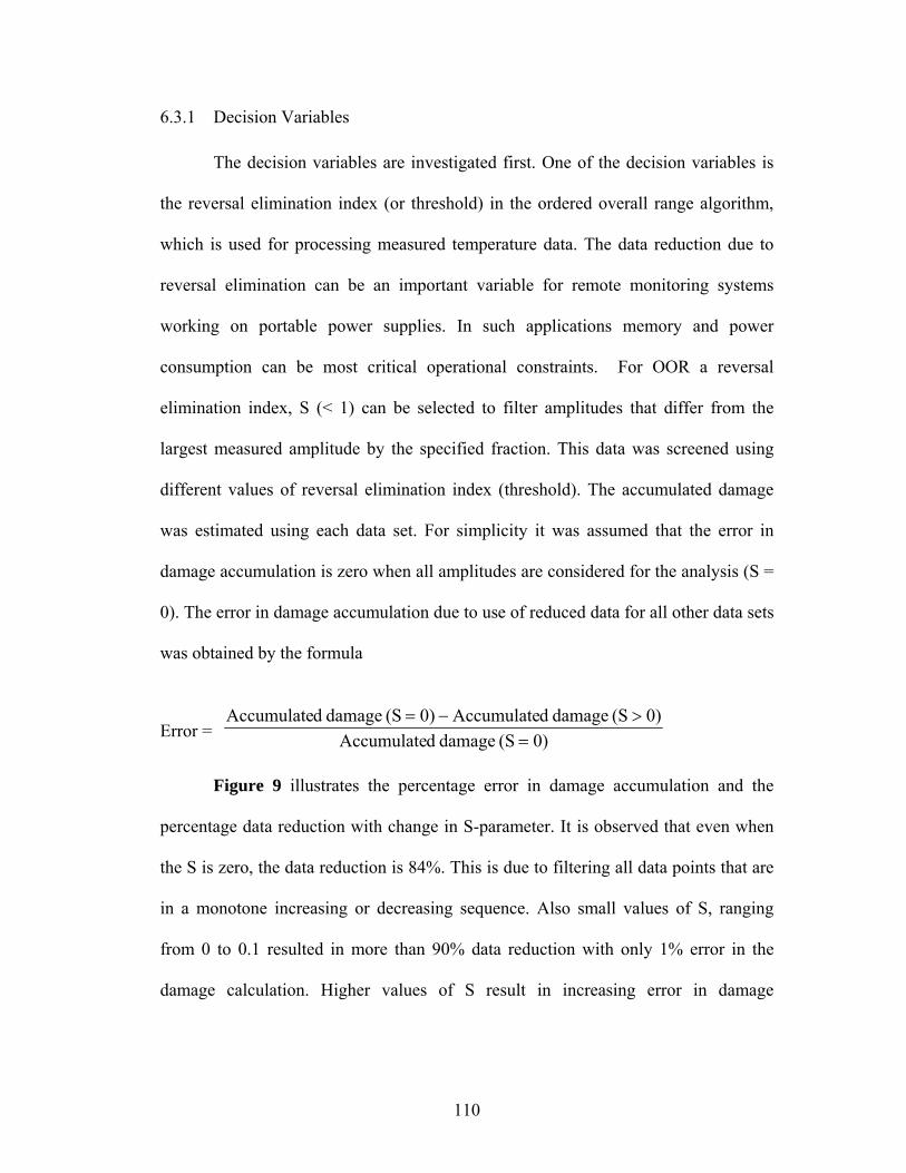
110
6.3.1 Decision Variables
The decision variables are investigated first. One of the decision variables is
the reversal elimination index (or threshold) in the ordered overall range algorithm,
which is used for processing measured temperature data. The data reduction due to
reversal elimination can be an important variable for remote monitoring systems
working on portable power supplies. In such applications memory and power
consumption can be most critical operational constraints. For OOR a reversal
elimination index, S (< 1) can be selected to filter amplitudes that differ from the
largest measured amplitude by the specified fraction. This data was screened using
different values of reversal elimination index (threshold). The accumulated damage
was estimated using each data set. For simplicity it was assumed that the error in
damage accumulation is zero when all amplitudes are considered for the analysis (S =
0). The error in damage accumulation due to use of reduced data for all other data sets
was obtained by the formula
Error = 0)(S damage dAccumulate0)(S damage dAccumulate0)(S damage dAccumulate
=>−=
Figure 9 illustrates the percentage error in damage accumulation and the
percentage data reduction with change in S-parameter. It is observed that even when
the S is zero, the data reduction is 84%. This is due to filtering all data points that are
in a monotone increasing or decreasing sequence. Also small values of S, ranging
from 0 to 0.1 resulted in more than 90% data reduction with only 1% error in the
damage calculation. Higher values of S result in increasing error in damage

111
accumulation. This is due to elimination of reversals with large magnitude and the
dependence of the fatigue model on the temperature amplitude.
Figure 37. Sources of uncertainty in damage estimation and prognostics for BGA225
Another example of analysis of decision variable is the download frequency.
The term download frequency denotes the number of times the monitoring system
was interrogated for checking the status or making predictions. Interrogating the
system more often results in breaking the data sets. Assuming the user is planning to
download on a periodic basis, the decision on download frequency can be made based
on analysis shown in Figure 38. Using the temperature data used for analysis in
Figure 9, the damage analysis was conducted by using the complete data sets,
breaking the data set into 3 parts, 5 parts and 10 parts. This is referred as signal
interruption on the y-axis of Figure 38. The error was normalized with respect to the
data set with no reversal elimination and signal interruptions. In this case all values
are low, also it seems like the error has started to become constant. i.e., there is a
Damage fractions
Component materials
Package substrate modulus
Overmoldmodulus & CTE
Board and solder materials
Board modulusBoard Poissons
ratioBoard CTE in
X & YSolder
properties
Board and solder joint geometry
Solder height
Collapsed ball height
Bond area
Board thickness
pad type
Component geometry
Package length
Package width
Package thickness
Overmoldthickness
Ball diameterDie length
Die widthDie thickness
Thermal loads with associated
uncertainties
Model parameters
Calibration constants
Fatigue coefficient
Model assumptions
and applicability
Ball span
Package substrate CTE
Damage fractions
Component materials
Package substrate modulus
Overmoldmodulus & CTE
Board and solder materials
Board modulusBoard Poissons
ratioBoard CTE in
X & YSolder
propertiesBoard and
solder materials
Board modulusBoard Poissons
ratioBoard CTE in
X & YSolder
properties
Board and solder joint geometry
Solder height
Collapsed ball height
Bond area
Board thickness
pad type
Component geometry
Package length
Package width
Package thickness
Overmoldthickness
Ball diameterDie length
Die widthDie thickness
Thermal loads with associated
uncertainties
Model parameters
Calibration constants
Fatigue coefficient
Model parameters
Calibration constants
Fatigue coefficient
Model assumptions
and applicability
Ball span
Package substrate CTE

112
large change between 0 to 3 days. However, the difference between 5-10 days is not
as much.
Figure 38. Error in damage accumulation due to reversal elimination and signal interruption
6.3.2 Model Parameters
Sensitivity analysis was conducted for the thermal fatigue model for BGA
225. The second column in Table 10 shows the change in the cycles to failure for a
one percent change in the input variable around the nominal value. These values are
then multiplied with the standard deviation of the model-input parameters, obtained
from manufacturer data, literature, and measurements. The normalized range
sensitivity index was calculated as shown in the approach (section 2). The final
column shows that the ranks are rearranged by considering the natural variability of
the model-input parameters. As per the new ranks, the top four model-input
0 0.025 0.050.075
0.1
03
5100.00
0.25
0.50
0.75
1.00
1.25
1.50
Fraction of largest cycle to be eliminated (data reduction)
# of signal interruptions
Nor
mal
ized
err
or*
in d
amag
e ac
cum
ulat
ion
due
to d
ata
redu
ctio
n an
d si
gnal
inte
rrup
tion
(%)
0 0.025 0.050.075
0.1
03
5100.00
0.25
0.50
0.75
1.00
1.25
1.50
Fraction of largest cycle to be eliminated (data reduction)
# of signal interruptions
Nor
mal
ized
err
or*
in d
amag
e ac
cum
ulat
ion
due
to d
ata
redu
ctio
n an
d si
gnal
inte
rrup
tion
(%)
Fraction of largest cycle to be eliminated (data reduction)
# of signal interruptions
Nor
mal
ized
err
or*
in d
amag
e ac
cum
ulat
ion
due
to d
ata
redu
ctio
n an
d si
gnal
inte
rrup
tion
(%)

113
parameters were assigned probability distributions and were used for in random
sampling for damage assessment.
Table 10. Sensitivity analysis of model-input parameters
Model Parameters % change in
predicted cycles to
failure*
Normalized
sensitivity index
Rank
Collapsed ball height 2.45 0.00295 3
Board CTE 2.20 0.00412 1
Component CTE 1.26 0.00321 2
Diagonal length 1.26 0.00139 4
Overmold thickness 0.57 0.00091 6
Overmold modulus 0.50 0.00075 7
Package substrate CTE 0.44 0.00101 5
Package substrate
modulus
0.19 0.00033 8
Pkg. substrate thickness 0.19 0.00028 9
6.3.3 Random Sampling
The four model-input parameters that were selected for Monte Carlo analysis
for the damage assessment of the BGA 225 included, coefficient of thermal
expansion (CTE) of the printed circuit board, CTE of component, collapsed solder
ball height, and diagonal length of the component. The normal distributions assigned
to each of these parameters are shown in Figure 39. The model-input parameter
distributions and the measured load parameter distributions were randomly sampled
using a Monte-Carlo technique within the damage model. The Monte-Carlo was
stopped when the standard error over the mean was less than 1 percent of the mean

114
value. The resulting data on damage fractions was analyzed using the procedure in
section 2 to obtain a distribution of accumulated damage. The stopping criteria of
stabilizing the variance over the mean were utilized. Typically it required 10,000 runs
of the Monte Carlo to satisfy this criterion (Figure 40).
Figure 39. Monte-Carlo simulation for damage assessment
6.3.4 Model Uncertainty
The model used in this study is the first order thermal fatigue model for plastic
ball grid arrays [117]. This model has been extensively used for various studies in
industry and academia. The studies have compared the cycles to failure of BGA
components obtained from accelerated testing with the results obtained from the
model (estimated). Using the approach presented in section 2, the distribution of yi
was derived using 48 data points obtained from CalcePWA manual for the model.
The distribution of yi was randomly sampled and used as a multiplicative constant
(Figure 41).
N (0.45, 0.004) N (14.8, 0.1) N (17, 0.5) N (13, 0.5)
Collapsed ball height Diagonal Length Board CTE Component CTE
0
5
0
5
0
∆T
Tmean
1st Order Thermal Fatigue Equation for BGA Solder Joints
Distribution after 10 days
Damage
Measured values over 10 days
0
300
600
900
0 0.003 0.006 0.009
Occ
urre
nce

115
Figure 40. Monte Carlo results and stopping criteria
Figure 41. Distribution of calibration parameter for model uncertainty
6.3.5 Remaining Life Prognostics
Using the regression analysis presented in section 2, the distribution of
accumulated damage after every ten days is shown in Figure 43. The actual failures
in testing were observed on day 87 and 92. Based on the failure criteria, the
remaining life prognostics are shown in Table 11. The first column shows the day on
which the prediction was made, which represents the monitoring period data that was
predictedf
measuredfi N
Ny
)()(
=
1.11.00.90.80.70.60.5
3.02.52.01.51.00.50.0
yi
Den
sity
µ = 0.79σ = 0.13 estimated
ii D
yD ⎟⎟
⎠
⎞⎜⎜⎝
⎛=
1
predictedf
measuredfi N
Ny
)()(
=
1.11.00.90.80.70.60.5
3.02.52.01.51.00.50.0
yi
Den
sity
µ = 0.79σ = 0.13
1.11.00.90.80.70.60.5
3.02.52.01.51.00.50.0
yi
Den
sity
µ = 0.79σ = 0.13 estimated
ii D
yD ⎟⎟
⎠
⎞⎜⎜⎝
⎛=
1

116
used for prognostics. The spread of the remaining life distribution decreases as the
time in use increases, i.e., the spread of the remaining life distribution made on day
60 is higher than the spread on day 84.
Figure 42. Accumulated damage distributions with time for BGA 225
Table 11. Remaining life distributions for BGA 225 Remaining life with probability Day of assessment
0.5% 50% 95%
60 24 32 37
72 15 20 22
84 1 5 9
6.3.6 Damage Histories for Prognostics
For products and systems operated over long durations, the accumulated
damage distribution can be stored in a condensed form. The user can track the change
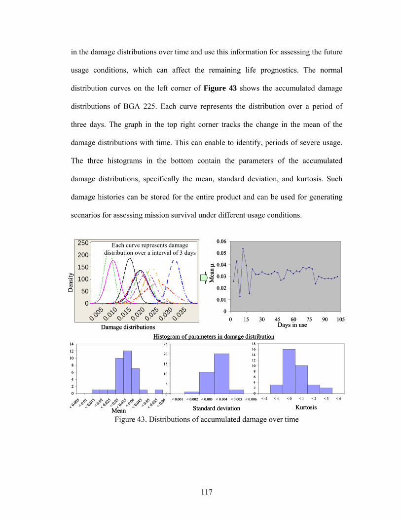
117
in the damage distributions over time and use this information for assessing the future
usage conditions, which can affect the remaining life prognostics. The normal
distribution curves on the left corner of Figure 43 shows the accumulated damage
distributions of BGA 225. Each curve represents the distribution over a period of
three days. The graph in the top right corner tracks the change in the mean of the
damage distributions with time. This can enable to identify, periods of severe usage.
The three histograms in the bottom contain the parameters of the accumulated
damage distributions, specifically the mean, standard deviation, and kurtosis. Such
damage histories can be stored for the entire product and can be used for generating
scenarios for assessing mission survival under different usage conditions.
Figure 43. Distributions of accumulated damage over time
0.035
0.030
0.025
0.020
0.015
0.010
0.005
250
200
150
100
50
0
Damage distributions
Den
sity
0
0.01
0.02
0.03
0.04
0.05
0.06
0 15 30 45 60 75 90 105Days in use
Mea
n µ
0
2
4
6
8
10
12
14
< 0.00
5< 0.
01
< 0.01
5< 0.
02
< 0.02
5< 0.
03
< 0.03
5< 0.
04
< 0.04
5< 0.
05
< 0.05
5< 0.
06
02468
1012141618
< -2 < -1 < 0 < 1 < 2 < 3 < 40
5
10
15
20
25
< 0.001 < 0.002 < 0.003 < 0.004 < 0.005 < 0.006
Mean Standard deviation Kurtosis
Histogram of parameters in damage distribution
Each curve represents damage distribution over a interval of 3 days

118
In the above experiment, each 3 day period can be considered as a mission.
The prognostic assessments can be conducted at the end of each mission to ensure the
number of failure free missions and the probability of surviving the next mission.
Also, the load distributions can be stored in compact format (per mission) and
retrieved for prognostic assessments when needed (Figure 44). The normal
distributions represent the distributions of delta T over each 3 day (mission) period.
The variations in the mean of the distributions over time are shown in the top right
graph of Figure 44. The two graphs in the bottom show the histograms for the mean
and standard deviation of the delta T distributions. The four graphs in Figure 43 can
be used to reconstruct the temperature loading history of the entire missions.
Figure 44. Condensed storage of load histories based on missions
Using the mission based approach, Table 12 shows the predicated mean
number of missions prior to failure. Two categories were considered. 1) The future
Delta T (degree C)
Den
sity
30025020015010050
0.008
0.006
0.004
0.002
0.000
120
130
140
150
160
170
180
190
200
0 5 10 15 20 25 30 35 40 45Missions
Mea
n of
∆T
dist
ribut
ion
Parameters of the Mission Load Distributions
mean
Freq
uenc
y
170160150140130
20
15
10
5
0
Standard deviation
Freq
uenc
y
7065605550454035
1816141210
86420

119
mission would be as severe as the mean value of all previous missions, and 2) the
future mission will have a severity value equivalent to the worst case severity based
on the previous missions. Actual failures were observed in mission 29 and 31.
Table 12. Remaining life prognostics in terms of missions
6.4 Conclusion
The sources of uncertainty in the prognostic approach based on environmental
and usage exposure were identified. A generic approach to prognostics that can
account for uncertainties in measurement, model-input, and damage models was
developed and demonstrated to provide a distribution of remaining life.
It was found that given the measurement, parameter and model uncertainties,
the actual failures in testing were observed within the predicted failure distribution.
The sensitivity analysis procedure revealed that it is important to consider the
standard deviation of parameter variables for calculating sensitivity indices, as it can
strongly influence the ranking of the most sensitive variables. Prognostic approach
consistently provided an advanced warning of failure for all components in the study.
1.12.727
0.61.828
0.9
3.6
Mission severity = mean
Predicted mean number of missions prior to failure at 95% C.I.
029
1.626
Mission severity = worst case
End of mission
1.12.727
0.61.828
0.9
3.6
Mission severity = mean
Predicted mean number of missions prior to failure at 95% C.I.
029
1.626
Mission severity = worst case
End of mission

120
It was observed that the prediction accuracy increased with the decrease in remaining
life. This was attributed to the fact that with increased usage there was more data to
support the prognostics.

121
Chapter 7: Failure Precursors Based on Resistance Analysis
7.0 Introduction
The previous four chapters discussed the methodology and case-studies for
prognostics based on monitoring and modeling of life cycle environmental and usage
loads. This chapter presents a different approach for prognostics using the same setup
described in chapter 3. Instead of assessing the accumulated damage due to
temperature cycles, the performance of the electronic board is directly monitored and
analyzed to provide an advance warning of failure and estimate remaining life. The
next few sections discuss the challenges in monitoring the performance, the
methodology adopted for analysis or failure precursors and the results.
The failure mode being investigated here is solder joint cracking, which can
introduce the complete fracture through the cross-section of the solder joint with the
solder joint parts having none or partial adhesion to each other. The failure
mechanism is creep and stress relaxation enhanced thermal fatigue due to temperature
cycling. A failed solder joint is normally surrounded by solder joints that have not yet
failed and therefore the solder joint fracture surfaces make compressively loaded
contact. During thermal changes shear is the primary force of stress on the solder
joints. As a result, the rough fractured surfaces of the failed solder joints slide
relative to one another producing characteristic short duration electrical transients.
There are several methods to detect solder joint failures, including destructive testing

122
to visually inspect cracks in the solder joints at periodic intervals, periodically
measuring the electrical resistance of solder joints and define the failures based on the
increase in original resistance, and continually monitoring electrical resistance of
solder joints to detect electrical discontinuities as failures.
As mentioned in chapter 3, the test board used in this experiment has 6
different components and two components of each type making totally 12
components on the board. All components have a daisy chain for monitoring
resistance continuity. A daisy chain is a conductive path that connects several
interconnections of a component. In this experiment a failure of any daisy chain
indicates the failure of the component. The daisy chain resistance of all components
except the QFP 100 was measured in-situ for the entire period of the experiment. The
QFP100 was not monitored in-situ, since the damage models and previous testing had
predicted that the component was not susceptible to failure under the given
conditions.
Thus in this experiment, the resistance of the daisy chains indicate the
performance of the component. The daisy chains have a base resistance before start of
the experiment. The daisy chain of the BGAs and QFPs extended onto the pads on the
printed circuit board. Wires were soldered onto the pad and connected to an Agilent
Model: 34970A data logger to take measurements of resistance every ten seconds.
The base resistance of the daisy chain was measured and recorded prior to thermal
cycling exposure. The data logger was operated in constant current mode at a source

123
current of 1mA, which passes through the daisy chains and reports the resistance of
the path.
The plot of resistance versus days in testing is shown in Figure 45. As the
component approaches failure, the short duration electrical spikes are observed in the
resistance values. After the first spike the subsequent spikes occur within a short
duration of time and ultimately the solder joint shows a complete open (infinite
resistance). It is evident from the Figure 45 that just by monitoring the resistance it is
impossible to provide any indication of degradation prior to the occurrence of the first
spike. The question asked here is that can we identify and estimate a degradation
trend even before the occurrence of the first spike?
Figure 45. No indication of degradation before the occurrence of the first spike
Additionally, the challenge to identify a degradation trend is further
complicated due to the constant change in resistance values during thermal cycling.
The resistance increases with increase in temperature and returns back to normal as
-100
10203040506070
0 400 800 1200 1600 2000 2400 2800 3200 3600Time (Hours)
Res
ista
nce
(ohm
s)

124
shown in Figure 46. This is a typical representation for component PBGA 225.
However, the change in the temperature-resistance is dependant on the component,
base resistance, temperature cycle, and also the damage accumulation of the
component. For example, the change in resistance for a temperature cycle with ∆T of
100oC is higher after 1000 cycles as compared to the start of the experiment. With
continued thermal cycling the daisy chain resistance will gradually increase to
indicate failure (crack growth leading to open connection), as shown in Figure 45.
The resistance will increase with initial spikes and eventually lead to complete open
with infinite resistance.
Figure 46. Change in resistance with temperature

125
7.1 Approach
Based on the above discussion there are two important issues: (1) the
identification of resistance degradation trend before the occurrence of first spike and
(2) the effect of temperature variations on resistance. The approach used to resolve
both issues and enable the identification of the onset of degradation is shown in
Figure 47.
Figure 47. Approach for precursor identification and tracking using resistance drift values
The core of the approach is the relationship between temperature and
resistance R = F(T), which is developed using in-situ monitored temperature and
resistance data at the beginning of the experiment. This is equivalent to establishing a
base-line performance. Since all components are in almost pristine condition, using
this relationship, the resistance can be predicted as a function of temperature. Thus as
the testing continues, the actual resistance R(T) is measured and recorded for the
)(TfR =
In-situ Monitoring
Temperature (T) Resistance R(T)
Resistance drift (D) = Re(T) – R(T)
Analyze features from distributions of resistance drifts
Estimated resistance Re(T)
Trend features to predict failure
)(TfR = )(TfR =
In-situ Monitoring
Temperature (T) Resistance R(T)
Resistance drift (D) = Re(T) – R(T)
Analyze features from distributions of resistance drifts
Estimated resistance Re(T)
Trend features to predict failure

126
component. Also, based on the temperature – resistance (TR) relationship, a value of
resistance is estimated Re(T). The actual resistance value is then subtracted from the
estimated value in time domain, to provide a resistance drift (D).
The resistance drift indicates a deviation from the expected normal condition.
However, the values of drift in time domain also produce a noisy signal and cannot be
directly used for identifying a degrading trend. Hence the values of drift are analyzed
over windows of ten hours. Using these values on can track the shift in the
distribution of drift values. Also the ten hour window covers the longest temperature
cycle that can be observed in the experiment. Using the ten hour resistance drift data,
various features were analyzed to identify the best (reliable) feature that can be used
as a prognostic indicator. Failure criteria were set to 50% increase in the mean of the
drift distribution. The 50% increase also corresponds to the first large spike that was
measured during resistance monitoring.
7.1.1 Temperature – Resistance Model
A second order polynomial was fitted to predict the change in resistance with
temperature. The coefficients α1, α2, and α3 were calculated based on the first 3600
data points, with the corresponding 95% confidence intervals.
R = f(T) = α1T2 + α2T + α3
The fit for component QFP 256 is shown in Figure 48, the details of the fit are shown
in Figure 49. Table 13 gives the mean and 95% confidence values for α1, α2, and α3.
The R2 value for the fit is 98.9%. As observed from Figure 49, the residual values
follow a normal distribution with a mean zero. The residual values are evenly
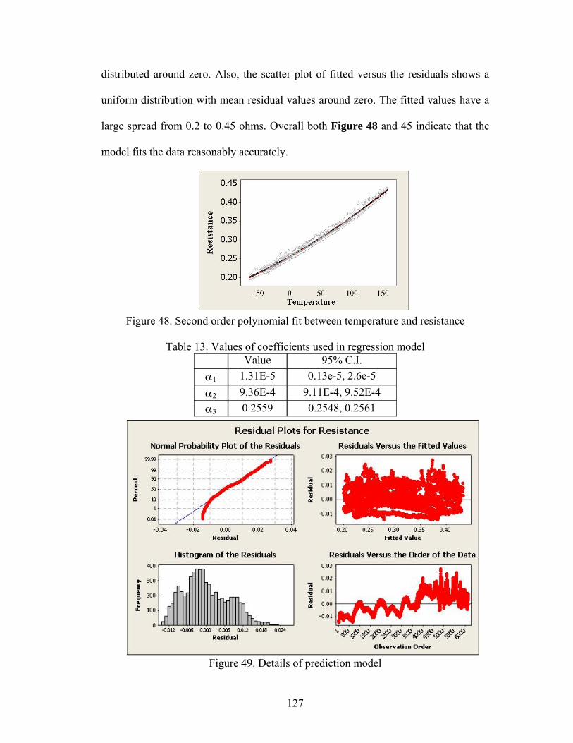
127
distributed around zero. Also, the scatter plot of fitted versus the residuals shows a
uniform distribution with mean residual values around zero. The fitted values have a
large spread from 0.2 to 0.45 ohms. Overall both Figure 48 and 45 indicate that the
model fits the data reasonably accurately.
Figure 48. Second order polynomial fit between temperature and resistance
Table 13. Values of coefficients used in regression model Value 95% C.I. α1 1.31E-5 0.13e-5, 2.6e-5 α2 9.36E-4 9.11E-4, 9.52E-4 α3 0.2559 0.2548, 0.2561
Figure 49. Details of prediction model

128
7.1.2 Features Investigated
The values of resistance drift and the features of the drift distributions over a
ten hour period were monitored and analyzed to identify which features could be
consistently used as a precursor to failure. The list of all feature investigated is shown
in Table 14.
Table 14. Features investigated for determining consistent precursor Feature Formula
Resistance drift D = Re(T) – R(T)
Mean drift values ∑ iD
n1
Mean peaks [ ] )(*,*, iDMaxDDt =
Standard deviation ( )21 DDN i −
95% cumulative distribution values F0.95(D)
95% cumulative peaks [F0.95]i*, (F0.95)*i = Max (F0.95)i
Skewness
Skewness peaks [ ] )(*,*, iii SMaxSSt =
Kurtosis
Kurtosis peak [ ] )(*,*, iKMaxKKt =
Third quartile 75th Percentile
Over a period of ten hours the data was collected and the features listed in
Table 14 were calculated. The feature values were plotted on a time scale to identify
if there is any observable trend. This procedure was conducted using data for all the
components on board (except for QFP 100). The objective was to find: (1) a
2/3
1
2
1
3 /)(/)( ⎥⎦
⎤⎢⎣
⎡−⎥
⎦
⎤⎢⎣
⎡− ∑∑
==
n
i
n
inDDnDD
2
1
2
1
4 /)(/)( ⎥⎦
⎤⎢⎣
⎡−⎥
⎦
⎤⎢⎣
⎡− ∑∑
==
n
i
n
inDDnDD

129
feature(s) that could be most reliable used for prognostics. Here the word reliable is
used to indicate a degree of confidence, and (2) feature(s) that provided degradation
trend across all components being investigated.
7.2 Results
Using the procedure in the previous section the results for QFP 256 are shown
in Figure 50 to 54. The following observations could be made about trending the
different features. The values of resistance drift by itself were too noisy for trending
and would lead to false alarms. The mean values of resistance drift distribution over a
ten hour period were found to provide a good indication of degradation. As seen in
Figure 46, for the component QFP 256, the mean drift values are close to zero or very
low for the first 200 hours. This indicates that the data fits to the regression model
and there is no deviation from the baseline performance.
Figure 50. Trending mean values of resistance drift
0
0.1
0.2
0.3
0.4
0.5
0 200 400 600 800 1000 1200 1400
Time (hours)
Res
ista
nce
Drif
t
First large spike
0
0.1
0.2
0.3
0.4
0.5
0 200 400 600 800 1000 1200 1400
Time (hours)
Res
ista
nce
Drif
t
First large spikeFirst large spike

130
After 200 hour to 500 hours, the value of mean drift fluctuates between zero
to 0.7. However, after 500 hours a steep rise is observed, with a clear increasing
trend. This would indicate a onset of fault and possible progression to failure. The
mean drift value was found to be the most consistent feature across all components
with similar trend. Figure 51, trends only the peak values of the mean drift (Figure
50). This is a better feature as there is no up or down trend (as observed with mean
drifts and also few other features). The peaks are always increasing and hence the
indication of degradation is clear.
Figure 51. Trending mean-peak values of resistance drift
Figure 52, 51, and 52 show the standard deviation, skewness, and kurtosis
values of the resistance drift. There is no change in the standard deviation values of
the drift as the component approaches failure. One would expect that the standard
deviation would increase with the mean (Figure 50), but it was not observed from the
data. Skewness and kurtosis were considered to describe the drift distributions more
accurately. High positive skewness values would indicate that the drift distribution is
0
0.1
0.2
0.3
0.4
0.5
0 200 400 600 800 1000 1200 1400
Time (hours)
Res
ista
nce
Drif
t
First large spike
0
0.1
0.2
0.3
0.4
0.5
0 200 400 600 800 1000 1200 1400
Time (hours)
Res
ista
nce
Drif
t
First large spikeFirst large spike

131
getting skewed to the right, indicating more number of large positive drift values.
However, for this component skewness values were not found to be a good indicator
of degradation. Though, the peak skewness values (Figure 57) show a consistent
increasing trend, it is difficult to use this trend directly, especially since the
component failure is not defined in terms of skewness.
Figure 52. Trending values of standard deviation of resistance drift
The 95 percent cumulative distribution values of the resistance drift were
found to be a good indicator of onset and progression of degradation. The progression
of 95% cumulative values is similar to that observed for the mean values. The data
(Figure 53) is characterized with low or no degradation till 200 hours followed by
slow increase till 500 hours, and the final rise to eventual failure. Similar to mean
peaks, the 95% cumulative peak values was found to be a good indicator for
degradation indication. This is primarily because the peaks only capture the
increasing values of the curve and hence it is easier to interpret. When similar
exercise was performed with data for all components on the board, the mean drift,
0
0.1
0.2
0.3
0.4
0.5
0 200 400 600 800 1000 1200 1400
Time (hours)
Res
ista
nce
Drif
t First large spike
0
0.1
0.2
0.3
0.4
0.5
0 200 400 600 800 1000 1200 1400
Time (hours)
Res
ista
nce
Drif
t First large spikeFirst large spike

132
mean peaks, 95% cumulative and cumulative peaks were found to be more robust
features for prognostics.
Figure 53. Trending values of 95% cumulative distribution values of resistance drift
0
0.1
0.2
0.3
0.4
0.5
0.6
0 200 400 600 800 1000 1200 1400
Time (hours)
Res
ista
nce
Drif
t
First spike
Figure 54. Trending values of 95% cumulative distribution peaks of resistance drift
0
0.1
0.2
0.3
0.4
0.5
0 200 400 600 800 1000 1200 1400
Time (hours)
Res
ista
nce
Drif
t
First large spike
0
0.1
0.2
0.3
0.4
0.5
0 200 400 600 800 1000 1200 1400
Time (hours)
Res
ista
nce
Drif
t
First large spike
First large spike

133
Figure 55. Trending skewness values of resistance drift
Figure 56. Trending kurtosis values of resistance drift
-1
0
1
2
3
4
5
0 200 400 600 800 1000 1200 1400
Time (hours)
Res
ista
nce
Drif
t First large spike
-1
0
1
2
3
4
5
0 200 400 600 800 1000 1200 1400
Time (hours)
Res
ista
nce
Drif
t First large spikeFirst large spike
-2
-1
0
1
2
3
4
5
0 200 400 600 800 1000 1200 1400
Time (hours)
Res
ista
nce
Drif
t
First large spike
-2
-1
0
1
2
3
4
5
0 200 400 600 800 1000 1200 1400
Time (hours)
Res
ista
nce
Drif
t
First large spikeFirst large spike

134
Figure 57. Trending skewness peak values of resistance drift
The mean peaks and 95% cumulative distribution peaks were fitted using
linear regression to predict the failure (Figure 58). The prediction obtained after 950
hours using mean values of the drift distribution was 1780 hours. The prediction
obtained using 95% cumulative distribution values was 1210 hours. The actual
measured failure was at 1300 hours. The actual failure could be enveloped by
trending these two features.
0
1
2
3
0 200 400 600 800 1000 1200 1400
Time (hours)
Res
ista
nce
Drif
t
First large spike
0
1
2
3
0 200 400 600 800 1000 1200 1400
Time (hours)
Res
ista
nce
Drif
t
First large spikeFirst large spike

135
Figure 58. Failure prediction using two features
7.3 Conclusions
A novel approach was developed for predicting interconnect failure using in-
situ resistance measurements. Resistance drift was identified as a primary indicator of
health. The deviation of resistance drift from the established baseline was investigated
using different features. The mean and the 95% cumulative values of the resistance
distribution were identified as the most robust features for indicating degradation. The
onset of degradation and the progression to failure could be explained using the mean
values of resistance drift. For prognostics, the 95% cumulative peak trend always
provided advanced warning of failure. The actual failures (measured) were observed
between the failure prediction obtained from trending the mean peaks and 95%
cumulative peak values.
-0.1
0
0.1
0.2
0.3
0.4
0.5
0.6
0 200 400 600 800 1000 1200 1400
Time (hours)
Res
ista
nce
Drif
t 95% peaks
Mean peaks
Actual failure-0.1
0
0.1
0.2
0.3
0.4
0.5
0.6
0 200 400 600 800 1000 1200 1400
Time (hours)
Res
ista
nce
Drif
t 95% peaks
Mean peaks
Actual failure

136
Chapter 8: Contributions
The application of environmental and usage monitoring for health assessment
of mechanical systems has been well studied. However, these concepts have rarely
been applied for electronic products and systems. Electronics prognostics is evolving,
but most solutions are still in design concepts, prototypes, and product-specific
configurations. There are few actual realizations and even fewer commercialized
solutions.
The specific contributions of this research include the development and
demonstration of the algorithm to extract load parameters (cyclic range, mean loads,
ramp rates, dwell times) required for assessing damage due to commonly observed
failure mechanisms in electronics. The algorithm enables significant reduction of
large irregular time-load data without compromising features such as load-dwell
periods and small cycles with higher mean-load values that are essential for damage
estimation.
The unique feature of this algorithm is the identification of dwell times and
corresponding load levels by considering cycles with small amplitudes and cycles
with lower ramp rates. The method also estimates the correlation between load
parameters (cyclic range vs. mean, dwell time vs. load, cyclic range vs. ramp-rate)

137
using correlation coefficients to enable accurate damage assessment in subsequent
steps.
This research is first to utilize the methods of optimal binning and non-
parametric density estimation for prognostics and health management applications.
Method to enable condensed storage of in-situ monitored loads was demonstrated
using a-priori assessment of optimal bins for storage of load parameters. The binned
data was used with Gaussian kernel functions to estimate the probability density of
the load parameter. The method has shown to improve the ability of the sensor nodes
to monitor for extended durations without interruptions and conserve on-board
memory of sensor modules.
A generic approach for prognostics was proposed that accounted for
measurement, parameter, and model uncertainties. This novel approach combines
sensitivity analysis, Monte Carlo simulation, and regression modeling to predicting
the distribution of remaining life. The approach was demonstrated for predicting the
remaining life of solder interconnect failures on electronic boards under irregular
thermal loading conditions. Methods were proposed for predicting the remaining life
based on current and historic loads by utilizing the variations in the load distributions
with time to assess future usage patterns and mission survivability.
An approach for remaining life prognostics of electronic components due to
interconnect degradation by analyzing usage loads (temperature cycles) and

138
performance (resistance continuity) data was developed. The novel approach was
based on a regression model for predicting the resistance using measured temperature
values. The difference between actual and estimated resistance was then analyzed to
predict the onset and progress of degradation. The method was shown to accurately
predict remaining life by trending several features including means, mean peaks,
kurtosis, and 95% cumulative values of the resistance drift distributions.

139
Appendix I
Flow chart of the load parameter extraction algorithm.
Input discrete signal T(t) matrix of n X 2 values
∑−+
=)1(
1 )(1)(an
ntT
atT
[Tj – Ti] => (∆T)s
i = 2 n-1 and j = 3 n-2
next j
Append matrix of [tj, Tj]
next i
Monotonic condensation (MC) on new matrix of [t, T]
i = 2 n-1
∆Ti = Ti+1 - Ti , ∆ti = ti+1 –ti
[∆T]i <= [∆T]s (∆T/∆t)i <= (∆T/∆t)s
Retain [∆T]i
Update matrix based on residual [t, T]
Create new matrix of dwell time and temperature
[Ti, ∆ti]
MC on new matrix of [t, T]
Append matrix of full cycles ∆T, (Tmean)i = (Ti+1 – Ti)/2 ,
(∆T/ ∆ t)i = (Ti+1 – Ti)/(ti+1 – ti)
Convert residual matrix to half cycles
Update t-s matrix by shifting the existing stack
MC for new [t,T] matrix
(∆T)i > (∆T)i+1 ≤ (∆T)i+2
Check if full cycle = 0
END
Y
N
Start with residual
time-load stack
i = 2 n-1
N
Y
Y
N
Y
N
Y
Add to full cycle stack
tT
iitimedwell SS
tT
∆−
∆=
),cov(ρ
mTT
imimeanrange SS
TT
∆−
∆=
),cov(ρ
tTT
iiraterange SS
tTT
∆∆∆−
∆∆∆=
/
])/(,cov[ρ
Input discrete signal T(t) matrix of n X 2 values
∑−+
=)1(
1 )(1)(an
ntT
atT ∑
−+=
)1(1 )(1)(
an
ntT
atT
[Tj – Ti] => (∆T)s[Tj – Ti] => (∆T)s
i = 2 n-1 and j = 3 n-2
next j
Append matrix of [tj, Tj]
next i
Monotonic condensation (MC) on new matrix of [t, T]
i = 2 n-1
∆Ti = Ti+1 - Ti , ∆ti = ti+1 –ti
[∆T]i <= [∆T]s[∆T]i <= [∆T]s (∆T/∆t)i <= (∆T/∆t)s(∆T/∆t)i <= (∆T/∆t)s
Retain [∆T]i
Update matrix based on residual [t, T]
Create new matrix of dwell time and temperature
[Ti, ∆ti]
MC on new matrix of [t, T]
Append matrix of full cycles ∆T, (Tmean)i = (Ti+1 – Ti)/2 ,
(∆T/ ∆ t)i = (Ti+1 – Ti)/(ti+1 – ti)
Convert residual matrix to half cycles
Update t-s matrix by shifting the existing stack
MC for new [t,T] matrix
(∆T)i > (∆T)i+1 ≤ (∆T)i+2(∆T)i > (∆T)i+1 ≤ (∆T)i+2
Check if full cycle = 0Check if full cycle = 0
END
Y
N
Start with residual
time-load stack
i = 2 n-1
N
Y
Y
N
Y
N
Y
Add to full cycle stack
tT
iitimedwell SS
tT
∆−
∆=
),cov(ρ
mTT
imimeanrange SS
TT
∆−
∆=
),cov(ρ
tTT
iiraterange SS
tTT
∆∆∆−
∆∆∆=
/
])/(,cov[ρ

140
Appendix II Models for Damage Estimation and Accumulation used for Assessing Solder Joints
First order thermal fatigue model for BGAs and gull wing QFPs was used for
damage calculations. The model used contains all the first order parameters
influencing the shear fatigue life of solder joints and comes from the fundamental
understanding of the response of surface mount solder joints to cyclically
accumulating fatigue damage resulting from shear displacement due to thermal
expansion mismatches between the components and the substrate. These shear
displacements, the global thermal expansion mismatch, cause time independent
yielding strains, and time, temperature, and stress dependant creep/stress relaxation
strains. These strains, on a cyclic basis form a visco-plastic stain energy hysteresis
loop which characterizes the solder joints response to thermal cycling and those areas
is indicative of the cyclically accumulating fatigue damage.
⎟⎟
⎠
⎞
⎜⎜
⎝
⎛ ∆=
ε
γ
221
1
f
p cfN
Nf = Mean number of cycles to failure
∆γp = Inelastic strain range considering the local and global mismatch.
εf and c are material constants
For eutectic solder, εf = 0.325
⎟⎟⎠
⎞⎜⎜⎝
⎛++−−=
tTc
Dsj
360101740000604420 ln...
Where, Tsj = cyclic mean temperature of the solder in degrees C and tD =
dwell time in minutes at maximum temperature. . In the fatigue model, the ramp time

141
is considered in calculating the mean cyclic temperature, using the following
expression
Where,
τmax = Dwell time at maximum temperature
τmin = Dwell time at minimum temperature
τrampup = Ramp time from maximum to minimum temperature
τrampdown = Ramp time from minimum to maximum temperature
For BGAs the inelastic strain range due to global mismatch is given by
hTLTLFI cs
g)(. αα
γ∆−∆
=∆50
Where, I is the calibration factor internal to the software program. F =
empirical factor “non-ideal” factor that accounts for deviation of real solder joints
from ideal solder joints. h (mils) is the nominal height of the solder joints. Ts and Tc
are temperatures of the substrate and component.
Similarly for gull wing QFPs the inelastic strain range due to global mismatch
is given by
AhTLTLKFI csD
g 200)(5.0 2αα
γ∆−∆
=∆
Where, KD is the diagonal flexural lead stiffness for the gull wings based on
the work of Kotlowitz and Taylor [1991].
The package geometries namely, the size, shape, and areas of the solder balls
and the gull wing interconnects were supplied by the manufacturer. Some of these
values were verified by actual measurement. The material properties of solder, board,
( ) ( ) ( )( )ττττ
ττττ
rampdownrampup
rampdownrampups
TTTTT
+++
+×+
+×+×=
minmax
maxminminminmaxmax ])
2[(

142
interconnect, and packages were obtained from the manufacturer. For routinely used
materials such as Pb-Sn solder, and FR-4, these properties are stored in the database
of the custom software (CalcePWA) that was used for building the model. These
properties have been derived from several experimental results and from literature.
Damage Accumulation
Liner damage rule by Miner was used for damage accumulation. The
basic assumptions of this rule are constant work absorption per cycle and
characteristic amount of work absorbed at failure. The energy accumulation, therefore
leads to linear summation of cycle ratio or damage.
Damage ∑ ∑==fii
Nn
irD
Where, ni = applied cycle at load of constant amplitude i
Nfi = total cycle to failure at load i
Failure is deemed to occur when, ∑ = 1ir

143
Appendix III Publications Originated from Thesis Work
Journals • Vichare, N., Pecht, M., “Prognostics and Health Management of Electronics”,
IEEE Transactions on Components and Packaging Technologies, Vol. 29, No. 1, March 2006, pp.222-229.
• Vichare, N., Rodgers, P., Pecht, M., “Methods for Binning and Density Estimation of Load Parameters for Prognostics and Health Management”, International Journal of Performability Engineering, Vol. 2, No. 2, April 2006, pp.149-161.
• Vichare N., Rodgers P., Eveloy V., Pecht M. G., “In-Situ Temperature Measurement of a Notebook Computer - A Case Study in Health and Usage Monitoring of Electronics”, IEEE Transactions on Device and Materials Reliability, vol. 4., No. 4, December 2004, pp. 658-663.
• Vichare N., Rodgers P., Eveloy V., Pecht M. G., “Environment and Usage Monitoring of Electronic Products for Health Assessment and Product Design”, Accepted in the Journal of Quality Technology and Quantitative Management.
Conference Proceedings • Vichare N., Rodgers P., Eveloy V., Pecht M. G., “Environment and Usage
Monitoring of Electronic Products for Health (Reliability) Assessment and Product Design”, IEEE Workshop on Accelerated Stress Testing and Reliability, Austin, Texas, Oct 3-5, 2005.
• Rouet, V., Foucher, B., Vichare, N., Rodgers, P., and Pecht M., “Improvement of a Miniaturized Health Monitoring Device for Advanced Alerts”, International Conference on Condition Monitoring and Diagnosis, Changwon, Korea, April 2-5, 2006.
• Vichare N, and Pecht, M., “Enabling Electronic Prognostics Using Thermal Data”, Thermal Investigation of IC’s and Systems (THERMINIC), September 2006.
• Vichare, N., Rodgers, P., Azarian, M., and Pecht, M., “Application of Health Monitoring to Product Take-back Decisions”, Proceedings of the Joint International Congress and Exhibition - Electronics Goes Green 2004, 6-8 September 2004, Berlin., Germany, pp. 945-951, 2004.
Working Papers
• Vichare, N. M., and Pecht, M., G., Load parameter Extraction Algorithm for Prognostic Health Monitoring
• Vichare N., Rodgers P., Pecht M. G., Prognostic Health Monitoring Approach for Electronics Considering Uncertainty
• Vichare N., Pecht M., Zhang, G., Kwan, C., Prognostics Using Resistance Drift as Failure Precursor

144
Bibliography [1]. Vichare, N., Pecht, M., “Prognostics and Health Management of
Electronics”, IEEE Transactions on Components and Packaging Technologies, Vol. 29, No. 1, March 2006, pp. 222-229.
[2]. Vichare, N.; Rodgers, P., Eveloy, V., Pecht, M., “Monitoring Environment and Usage of Electronic Products for Health Assessment and Product Design”, IEEE Workshop on Accelerated Stress Testing and Reliability (ASTR), Austin, TX, USA, October 2-5, 2005.
[3]. Lall, P., Pecht, M., and Hakim, E., “Influence of Temperature on Microelectronics and System Reliability”, CRC Press, New York, 1997.
[4]. Pecht, M., Das, D., and Ramakrishnan, A., “The IEEE Standards on Reliability Program and Reliability Prediction Methods for Electronic Equipment,” Microelectronics Reliability, Vol. 42, 2002, pp. 1259-1266.
[5]. Dasgupta, A., “The Physics-of-Failure Approach at the University of Maryland for the Development of Reliable Electronics,” in Proceedings of Third International Conference on Thermal and Mechanical Simulation in (Micro) Electronics (EuroSimE), pp. 10-17, 2002.
[6]. Tumer, I., and Bajwa, A., “A Survey of Aircraft Engine Health Monitoring Systems”, Proceedings of AIAA, 1999.
[7]. Carden, E. P., Fanning, P., “Vibration Based Condition Monitoring: A Review”, Journal of Structural Health Monitoring, Vol. 3, No. 4, 2004, pp. 355-377.
[8]. Chang, P., Flatau, A., and Liu, S., “Review Paper: Health Monitoring of Civil Infrastructure”, Journal of Structural Health Monitoring, Vol 3, No. 3, 2003, pp. 257-267.
[9]. Krok, M., and Goebel, K., “Prognostics for Advanced Compressor Health Monitoring”, Proceedings of SPIE, Vol. 5107, 2003.
[10]. Kacprzynski, G. J., Roemer, M.J., Modgil, G., Palladino, A., “Enhancement of Physics of Failure Prognostic Models with System Level Features”, IEEE Aerospace Conference Proceedings, Vol. 6, 2002, pp. 2925.
[11]. Xie, J., and Pecht, M., “Application of In-Situ Health Monitoring and Prognostic Sensors,” 9th Pan Pacific Microelectronics Symposium Exhibits & Conference, Kahuku, Oahu, Hawaii, 10-12 February 2004.

145
[12]. Condition Based Maintenance Plus, http://www.acq.osd.mil/ log/mppr/CBM%2B.htm, Viewed December 2005.
[13]. DoD 5000.2 Policy Document, Defense Acquisition Guidebook, Chapter 5.3 – Performance Based Logistics, December 2004.
[14]. Cutter, D. and Thompson, O., “Condition-Based Maintenance Plus Select Program Survey,” Report LG301T6, January 2005, viewed from http://www.acq.osd. mil/log/mppr/CBM%2B.htm, October 2005
[15]. Kirkland, L.V.; Pombo, T.; Nelson, K.; and Berghout, F., “Avionics Health Management: Searching for the Prognostics Grail,” Proceedings of IEEE Aerospace Conference, Vol. 5, 6-13 March 2004, pp. 3448 – 3454.
[16]. Leonard, C.T. and Pecht, M.G., “Improved Techniques for Cost Effective Electronics,” Annual Proceedings of Reliability and Maintainability Symposium, 29-31 January 1991, pp. 174 – 182.
[17]. Karyagina, M., “Designing for Fault-Tolerance in the Commercial Environment,” Proceedings of Reliability and Maintainability Symposium, 22-25 January 1996, pp. 258 – 262.
[18]. Shapiro, A.A.; Ling, S.X.; Ganesan, S.; Cozy, R.S.; Hunter, D.J.; Schatzel, D.V.; Mojarradi, M.M.; and Kolawa, E.A., “Electronic Packaging for Extended Mars Surface Missions,” Proceedings of IEEE Aerospace Conference, Vol. 4, 6-13 March 2004, pp. 2515 - 2527.
[19]. Drees, R., and Young, N., “Role of BIT in Support System Maintenance and Availability,” IEEE A&E Systems Magazine, August 2004, pp. 3-7.
[20]. Pecht, M.; Dube, M.; Natishan, M.; and Knowles, I., “An Evaluation of Built-In Test,” IEEE Transactions on Aerospace and Electronic Systems, Vol. 37, No. 1, January 2001, pp. 266-272.
[21]. Motorola, “Motorola Built-In Test Diagnostic Software,” http://www.dot21rts.com/products/mbit%20datasheet.pdf, June 2002, Viewed on December 2005.
[22]. Broadwater, S.P.; Oblak, T.A.; and Popyack, L.J., “Maintenance Processor/Time Stress Measurement Device (MP/TSMD) Use for Failure Trend Analysis,” Annual Reliability and Maintainability Symposium, 1992, pp. 228-38.
[23]. Broadwater, S.P. and Cockey, E.A., “Time Stress Measurement Device Use for On-board Diagnostic Support,” Proceedings of IEEE AUTOTESTCON '93, September 1993, pp. 251-8.

146
[24]. Johnson, D., “Review of Fault Management Techniques Used in Safety Critical Avionic Systems,” Progress in Aerospace Science, Vol. 32, No. 5, October 1996, pp. 415-431.
[25]. Allen, D., “Probabilities Associated with a Built-in-Test System, Focus on False Alarms,” Proceedings of AUTOTESTCON, IEEE Systems Readiness Technology Conference, 22-25 September 2003, pp. 643 – 645.
[26]. Gao, R.X. and Suryavanshi, A., “BIT for Intelligent System Design and Condition Monitoring”, IEEE Transactions on Instrumentation and Measurement, Vol. 51, No. 5, October 2002, pp. 1061 – 1067.
[27]. Rosenthal, D. and Wadell, B., “Predicting and Eliminating Built-in Test False Alarms,” IEEE Transactions on Reliability, Vol. 39, No. 4, October 1990, pp. 500-505.
[28]. Williams, R., Banner, J., Knowles, I., Natishan, M., and Pecht, M., “An Investigation of 'Cannot Duplicate' Failure”, Quality and Reliability Engineering International, Vol. 14, 1998, pp. 331-337.
[29]. Ramakrishnan, A.; Syrus, T.; and Pecht, M., “Electronic Hardware Reliability.” Avionics Handbook, CRC Press, Boca Raton, Florida, December 2000, pp. 22-1 - 22-21.
[30]. Mishra, S. and Pecht, M., “In-situ Sensors for Product Reliability Monitoring,” Proceedings of SPIE, Vol. 4755, 2002, pp. 10-19.
[31]. Ridgetop Semiconductor-Sentinel Silicon ™ Library, “Hot Carrier (HC) Prognostic Cell,” August 2004.
[32]. Anderson, N. and Wilcoxon, R., “Framework for Prognostics of Electronic Systems,” Proceedings of International Military and Aerospace/Avionics COTS Conference, Seattle, WA, August 3-5, 2004.
[33]. Ganesan, S.; Eveloy, V.; Das, D.; and Pecht, M.G, “Identification and Utilization of Failure Mechanisms to Enhance FMEA and FMECA,” Proceedings of the IEEE Workshop on Accelerated Stress Testing and Reliability (ASTR), Austin, Texas, October 3-5, 2005
[34]. Born, F. and Boenning, R. A., “Marginal Checking - A Technique to Detect Incipient Failures,” Proceedings of the IEEE Aerospace and Electronics Conference, 22-26 May 1989, pp. 1880 – 1886.
[35]. Pecht, M.G., Radojcic, R., and Rao, G., “Guidebook for Managing Silicon Chip Reliability”, CRC Press, Boca Raton, FL, 1999.
147
[36]. Smith, P.A. and Campbell, D.V., “Practical Implementation of BICS for Safety-Critical Applications,” Proceedings of IEEE International Workshop on Current and Defect Based Testing-DBT, 30 April 2000 pp. 51 – 56.
[37]. Pecuh, I.; Margala, M.; and Stopjakova, V., “1.5 Volts Iddq/Iddt Current Monitor.” Proceedings of the IEEE Canadian Conference on Electrical and Computer Engineering, Vol. 1, 9-12 May 1999, pp. 472 – 476.
[38]. Xue, B. and Walker, D.M.H., “Built-In Current Sensor for IDDQ Test,” Proceedings of the IEEE International Workshop on Current and Defect Based Testing-DBT, 25 April 2004, pp. 3 – 9.
[39]. Wright, R.G. and Kirkland, L.V., “Nano-Scaled Electrical Sensor Devices for Integrated Circuit Diagnostics,” IEEE Aerospace Conference Proceedings, Vol. 6, Mar 8-15, 2003, pp. 2549 - 2555.
[40]. Wright, R.G.; Zgol, M.; Adebimpe, D.; and Kirkland, L.V., “Functional Circuit Board Testing Using Nanoscale Sensors,” IEEE Systems Readiness Technology Conference Proceedings AUTOTESTCON, 22-25 September 2003, pp. 266 – 272.
[41]. Wright, R.G.; Zgol, M.; Keeton, S.; and Kirkland, L.V., “Nanotechnology-Based Molecular Test Equipment (MTE),” IEEE Aerospace and Electronic Systems Magazine, Vol. 16, No.. 6, June 2001, pp. 15 – 19.
[42]. Kanniche, M.S. and Mamat-Ibrahim, M.R., “Wavelet based Fuzzy Algorithm for Condition Monitoring of Voltage Source Inverters,” Electronic Letters, Vol. 40, No. 4, February 2004.
[43]. Lall, P., Islam, N., Rahim, K., Suhling, J., Gale, S., “Leading Indicators-of-Failure for Prognosis of Electronic and MEMS Packaging,” Proceeding of Electronics Components and Technology Conference, Las Vegas, NV, pp. 1570-1578, June 1-4, 2004..
[44]. Lall, P., Islam, N., Suhling, J., “Prognostication and Health Monitoring of Leaded and Lead Free Electronic and MEMS Packages in Harsh Environments”, Proceedings of the 55th IEEE Electronic Components and Technology Conference, Orlando, FL, pp. 1305-1313, June 1-3, 2005.
[45]. Self-Monitoring Analysis and Reporting Technology (SMART), PC Guide, http://www.pcguide.com/ref/hdd/perf/qual/featuresSMART-c.html, viewed on August 30, 2005
[46]. Hughes, G.F., Murray, J.F., Kreutz-Delgado, K., Elkan, C., “Improved Disk-drive Failure Warnings”, IEEE Transactions on Reliability, Vol. 51, Issue 3, September 2002, pp. 350 – 357.

148
[47]. Gross, K., “Continuous System Telemetry Harness,” Sun Labs Open House, 2004, research.sun.com/sunlabsday/ docs.2004/talks/1.03_Gross.pdf, viewed in August 2005.
[48]. Whisnant, K.; Gross, K.; and Lingurovska, N., “Proactive Fault Monitoring in Enterprise Servers,” 2005 IEEE International Multi-conference in Computer Science and Computer Engineering, Las Vegas, NV, June 2005
[49]. Mishra, K. and Gross, K. C, “Dynamic Stimulation Tool for Improved Performance Modeling and Resource Provisioning of Enterprise Servers,” Proc. 14th IEEE International Symposium on Software Reliability Eng. (ISSRE’03), Denver, CO, November 2003.
[50]. Cassidy, K.; Gross, K. C.; and Malekpour, A., “Advanced Pattern Recognition for Detection of Complex Software Aging Phenomena in Online Transaction Processing Servers,” Proceedings of the International Performance and Dependability Symposium, Washington, DC, June 23 - 26, 2002.
[51]. Vaidyanathan, K. and Gross, K. C., “MSET Performance Optimization for Detection of Software Aging,” Proc. 14th IEEE International Symposium on Software Reliability Engineering (ISSRE’03), Denver, CO, November 2003.
[52]. Brown, D.; Kalgren, P.; Byington, C.; and Orsagh, R., “Electronic Prognostics – A Case Study Using Global Positioning System (GPS)," IEEE Autotestcon, 2005
[53]. Ramakrishnan, A. and Pecht, M., “A Life Consumption Monitoring Methodology for Electronic Systems,” IEEE Transactions on Components and Packaging Technologies, Vol. 26, No. 3, September 2003, pp. 625-634.
[54]. Mishra, S.; Pecht, M.; Smith, T.; McNee, I.; and Harris, R., “Remaining Life Prediction of Electronic Products Using Life Consumption Monitoring Approach,” Proceedings of the European Microelectronics Packaging and Interconnection Symposium, Cracow, June 16-18, 2002, pp. 136-142.
[55]. Mathew, S.; Das, D.; Osterman, M.; Pecht, M.G.; and Ferebee, R., ’’Prognostic Assessmsnt of Aluminum Support Structure on a Printed Circuit Board,” Accepted for publication in ASME Journal of Electronic Packaging, EP-05-1031
[56]. Shetty, V.; Das, D.; Pecht, M.; Hiemstra, D.; and Martin, S., “Remaining Life Assessment of Shuttle Remote Manipulator System End Effector,” Proceedings of the 22nd Space Simulation Conference, Ellicott City, MD, October 21-23, 2002

149
[57]. Vichare N., Rodgers P., Eveloy V., Pecht M. G., “Environment and Usage Monitoring of Electronic Products for Health Assessment and Product Design”, Accepted for publication in Journal of Quality Technology and Quantitative Management
[58]. Harchani, N.; Jimenez, F.; Almohamed, M.; Esteve, D.; and Courvoisier, M., “Time Stress Measurement Device: System Design and Synthesis”, Proceedings of the SPIE, Vol. 4051, 2000, pp. 337-48.
[59]. Rouet, V. and Foucher, B., “Development and Use of a Miniaturized Health Monitoring Device,” Proceedings of the IEEE International Reliability Physics Symposium, 2004, pp. 645-6.
[60]. Searls, D.; Dishongh, T.; and Dujari, P., “A Strategy for Enabling Data Driven Product Decisions Through a Comprehensive Understanding of the Usage Environment,” Proceedings of IPACK’01, Kauai, Hawaii, USA, July 8-13, 2001.
[61]. Herbst, G., “IBM’s Drive Temperature Indicator Processor (Drive-TIP) Helps Ensure High Drive Reliability,” IBM White Paper, http://www.hc.kz/pdf/drivetemp.pdf, viewed in September 2005.
[62]. Vichare N.; Rodgers P.; Eveloy V.; and Pecht M. G., “In-Situ Temperature Measurement of a Notebook Computer - A Case Study in Health and Usage Monitoring of Electronics,” IEEE Transactions on Device and Materials Reliability, Vol. 4., No. 4, December 2004, pp. 658-663.
[63]. Bodenhoefer, K., “Environmental Life Cycle Information Management and Acquisition – First Experiences and Results from Field Trials,” Proceedings of Electronics Goes Green 2004+, Berlin, September 5-8, 2004, pp. 541-546.
[64]. ELIMA Report, “D-19 Final Report on ELIMA Prospects and Wider Potential for Exploitation,” April 30, 2005, www.ELIMA.org, viewed in December 2005.
[65]. Skormin, V.A.; Gorodetski, V.I.; and Popyack, L.J., “Data Mining Technology for Failure Prognostic of Avionics,” IEEE Transactions on Aerospace and Electronic Systems, Vol. 38, No. 2, April 2002, pp. 388 – 403.
[66]. Mishra, S.; Ganesan, S; Pecht, M.; and Xie; J., “Life consumption monitoring for electronics prognostics,” Proceedings of the IEEE Aerospace Conference,.Vol. 5, March 6-13, 2004, pp. 3455 – 3467.

150
[67]. Orsagh, R.; Brown, D.; Roemer, M.; Dabney, T.; and Hess, A., “Prognostic Health Management for Avionics Power Supplies,” IEEE Aerospace Conference Proceedings, 2005
[68]. Goodman, D.; Vermeire, B.; Spuhler, P.; and Venkatramani, H., “Practical Application of PHM/Prognostics to COTS Power Converters,” IEEE Aerospace Conference, Big Sky, Montana, USA, March 5-12, 2005.
[69]. JEP 122B, Failure Mechanisms and Models for Semiconductor Devices, JEDEC Standard, August 2003.
[70]. JEP 148, Reliability Qualification of Semiconductor Devices Based on Physics of Failure Risk and Opportunity Assessment, April, 2004.
[71]. IPC-SM-785, “Guidelines for Accelerated Reliability Testing for Surface Mount Attachments”, IPC Standard, November 1992.
[72]. S. Bosworth, S.C. Hsu, and J. Polcari, “Exceptional performance from the development, qualification, and implementation of a silicone adhesive for bonding heatsinks to semiconductor packages,” IEEE Transactions on Components, Packaging and Manufacturing Technology – Part A, vol. 18, no. 1, pp. 94-100, 1995.
[73]. M.F. Ben Achour, A. Bar-Cohen, “Mechanical stress reduction in heat sink bond layers – a numerical feasibility study,” in Proc. Electronic Components Technology Conference (ECTC), pp. 307-315, 1999.
[74]. A. Kaisare, Z. Han, D. Agonafer, and K. Ramakrishna, “Prediction of effect of heat sink adhesive on mechanical reliability of a wire bonded plastic ball grid array package,” in Proc. Eighth Intersociety Conf. on Thermal and Thermomechanical Phenomena in Electronics Systems (ITHERM 2002), pp. 926-931, 2002.
[75]. V. Eveloy, P. Rodgers, C. Hillman, and M. Pecht, “Reliability of pressure sensitive adhesive tapes for heat sink attachment in air-cooled electronic assemblies,” IEEE Trans. on Device and Materials Reliability: Thermal Management for Reliability, December 2004.
[76]. Socie, D., Rainflow Cycle Counting: A Historical Perspective, pp. 3-10, The Rainflow Method in Fatigue, Butterworth-Heinemann, Oxford, 1991.
[77]. ASTM E-1049, Standard Practice for Cycle Counting in Fatigue Analysis, ASTM International Standard, 1997.
[78]. Holman, R., Liaw, P., Methodologies for Predicting Fatigue Life, Journal of Materials, July 1997, pp.46-51.

151
[79]. Rychlik, I., Rainflow Cycles in Gaussian Loads, Fatigue and Fracture of Engineering Materials and Structures, Vol. 15, no.1, 1992, pp. 57-72.
[80]. Anzai, H., Algorithm of Rainflow Method, The Rainflow Method in Fatigue, Butterworth-Heinmann, Oxford, pp 11-20, 1991.
[81]. Yigang, Z., Shijie, Z., Minaggo, Y., A Cycle Counting Method Considering Load Sequence, International Journal of Fatigue, Vol-15, no. 5, 1993, pp. 407-411.
[82]. Cluff, K., Barker, D., Robbins, D., and Edwards, T., “Characterizing the Commercial Avionics Thermal Environment for Field Reliability Assessment”, Proceedings-Institute of Environmental Sciences, pp. 50-57, 1996.
[83]. Brown, M.W., et al., “An Analysis of Mean Stress in Multiaxial Random Fatigue”, Fatigue and Fracture of Engineering Materials and Structures, Vol. 19, no. 2, pp. 323-333, 1996
[84]. Nagode, M., and Zingsheim, F., “An Online Algorithm for Temperature Influenced Fatigue Life Estimation: Strain Life Approach”, International Journal of Fatigue, Vol-26, 2004, pp. 155-161
[85]. Nagode, M., and Michael, H., “An Online Algorithm for Temperature Influenced Fatigue Life Estimation: Stress Life Approach”, International Journal of Fatigue, Vol-26, 2004, pp. 163-171
[86]. Mukhopadhyay, et al., Online fatigue creep monitoring system for high temperature components of power plants, International Journal of Fatigue, Vol. 23, 2001, pp. 549-560
[87]. Stubbington, C.A., and Pearson, S., “Effect of dwell on the growth of fatigue cracks in Ti-6Al-4V alloy bar”, Engineering Fracture Mechanics, vol.10, no.4, 1978. p. 723-56.
[88]. Cowles, B.A., Sims, D., Warren, J., “Evaluation of the Cyclic Behavior of Aircraft Turbine Disk Alloys”, NASA Report CR 159409, 1978.
[89]. Askoy S., Peng, Y., and Armstrong, H., “Thermal Fatigue Analysis of Air-Cooled Gas Turbine Nozzles”, ASME Pressure Vessels and Piping Conference, San Diego, 1987
[90]. Seshadri, R., “Design and Life Prediction of Furnace Tubes in Creep Range”, ASME Pressure Vessels and Piping Conference, San Diego, 1987

152
[91]. Goswami, T., “A New Dwell Sensitivity Damage Parameter”, Materials and Design, Vol. 25, 2004, pp. 191-197.
[92]. Goswami, T., “Dwell Sensitivity: Part I – Behavior and Modeling”, Mechanics of Material, Vol. 22. 1995, pp 105-130.
[93]. Wand, P., Data Based Choice of Histogram Bin Width, The American Statistician, Vol. 51, No. 1, pp.59-64, March 1997.
[94]. Izenman, A. J., Recent Developments in Non Parametric Density Estimation, Journal of American Statistical Association, Vol. 86, No. 413, pp.205-13, March 1991.
[95]. Scott, D., On Optimal and Data Based Histograms, Biometrika, Vol. 66, No. 3, pp. 605-10, 1979.
[96]. Freedman, D., P. Diaconis, On Maximum Deviation Between the Histogram and Underlying Density, Zeitschrift fur Wahrscheinlichkeitstheorie und verwandte Gebiete, 58, pp. 139-167, 1981.
[97]. He, K., G. Meeden, Selecting the Number of Bins in a Histogram a Decision Theoretic Approach, Journal of Statistical Planning and Inference, Vol. 61, No. 1, pp. 49-59, 1997.
[98]. Jones, M., J. Marron, S. Sheather, A Brief Survey of Bandwidth Selection for Density Estimation, Journal of American Statistical Association, Vol. 91, No. 433, pp.401-407, 1996.
[99]. Koyama, S., S. Shinomoto, Histogram Bin Width Selection for Time-Dependant Poisson Process, Journal of Physics A: Mathematics and General, Vol. 37, No. 29, pp. 7255-65, 2004.
[100]. Song, M., R., Haralick, Optimally Quantized and Smoothed Histograms, Proceedings of Joint Conference on Information Sciences, Computer Vision, Pattern Recognition and Image Processing, pp. 894, 2002.
[101]. Paulter, N.G., The Effect of Histogram Size on Histogram- Derived Pulse Parameters, IEEE Transactions on Instruments and Measurements, Vol. 47, No. 3, pp.609-12, 1998.
[102]. Silverman, B. W., Density Estimation for Statistics and Data Analysis, Chapman and Hall, New York, 1986.
[103]. Fadda, D., E. Slezak, A. Bijaoui, Density Estimation with Non-parametric Methods, Astronomy and Astrophysics Supplement Series, Vol. 127, pp. 335-52, January 1998.

153
[104]. Sheather, S., M. Jones, A Reliable Data Based Bandwidth Selection Method for Kernel Density Estimation, Journal of Royal Statistical Society, Vol. 53, No.3, pp.683-90, 1991.
[105]. Chiu, S., Bandwidth Selection for Kernel Density Estimation, Annals of Statistics, Vol. 19, No. 4, pp. 1883-1905, 1991.
[106]. Glavinovic, M., Comparison of Parzen Density and Frequency Histograms as Estimators of Probability Density Function, European Journal of Physiology, Vol. 433, No. 1-2, pp. 174-179, 1996.
[107]. Vichare, N., Rodgers, P., Pecht, M., Methods for Binning and Density Estimation of Load Parameters for Prognostics and Health Management, International Journal of Performability Engineering, Vol. 2, No. 2, April 2006, pp. 149-161.
[108]. Engel S. et al., Prognostics, The Real Issues Involved With Predicting Life Remaining, IEEE Aerospace Conference, vol.6, 2000, p. 457-69.
[109]. Ayyub, B., Uncertainty Modeling and Analysis for Civil Engineers, CRC Press, Boca Raton, 1998.
[110]. Frey, C., and Patil, S., Identification and Analysis of Sensitivity Analysis Methods, Risk Analysis, Vol. 22, No. 3, 2002.
[111]. Helton, J., and Davis, F., “Illustration of Sampling-Based Methods for Uncertainty and Sensitivity Analysis”, Risk Analysis, Vol. 22, No. 3, 2002
[112]. Zimmermann, H., An Application Oriented View Of Modeling Uncertainty”, European Journal of Operation Research, Vol. 122, pp. 190-198, 2000
[113]. Nilsen, T.; Aven, T, Models And Model Uncertainty In The Context Of Risk Analysis, Reliability Engineering & System Safety, Mar2003, Vol. 79 Issue 3, p309, 9.
[114]. Zio, E., Apostolakis, G.E., Two Methods For The Structured Assessment Of Model Uncertainty By Experts In Performance Assessments Of Radioactive Waste Repositories, Reliability Engineering & System Safety, v 54, n 2-3, Nov-Dec, 1996, p 225-241.
[115]. Banks, J., Carson, J., Nelson, B., and Nicol, D., Discrete Event System Simulation, 4th Edition, Prentice Hall, NJ, 2004.
[116]. Vose, D., Quantitative risk analysis: a guide to Monte Carlo simulation modeling, Chichester ; New York : Wiley, c1996.

154
[117]. Osterman, M., Qi, H., Explanation of First Order Thermal Fatigue Model for Solder Interconnects in Area Array Packages, CalcePWA Software Documentation, 2002.
[118]. P. Sharma, and A. Dasgupta, “Micro-mechanics of creep-fatigue damage in PB-SN solder due to thermal cycling—Part II: mechanistic insights and cyclic durability predictions from monotonic data,” Transactions of the ASME, Journal of Electronic Packaging, vol. 124, no. 3, pp. 298-304, 2002.
[119]. C. Zhai, Sidharth, and R. Blish, “Board level solder reliability versus ramp rate and dwell time during temperature cycling,” IEEE Transactions on Device and Materials Reliability, vol. 3, no. 4, December 2003, pp 207-212.
[120]. R. Mahajan, C.P. Chiu, and R. Prasher, “Thermal interface materials: a brief review of design characteristics and materials,” Electronics Cooling, vol. 10, no. 1, 2004.