abstract normalization an advanced concept of relational
TRANSCRIPT

ABSTRACT NORMALIZATION
An Advanced Concept of Relational Theory
by Les Cardwell
Copyright
-all rights reserved-

CHAPTER 1 Introduction
The basis for the theory on Abstract Normal Form (ANF) began in 1992 when I was introduced to what is now the second of the ANF constructs. This solution solved a problem for a Manufacturing/Accounting application, and was shared with me by a developer who had used the construct to solve a similar business problem for a For-tune 500 company. Through its most basic implementation, he was able to remove the 'run-time' transactional requirements from the order entry desk, yet maintain a 'real-time' Inventory, which was my goal as well.
Sometime in 1995, after having expanded on the basic construct to solve more complex database problems, I began looking for informa-tion to expand my knowledge of the subject. As it turned out, there was none. In September of 1996 I gave the first presentation on "Abstract Normalization" to the International DataEase Users Asso-ciation conference held in Wilmington Delaware. The response to that presentation has led to ongoing requests for further elucidation, which ultimately has led to this treatise.
Abstract Normalization : An Advanced Concept of Relational Theory 2

Introduction
3
During the development of LedgerMaster, a double-entry accounting package written in DataEase, there was a good deal of opportunity to press the concept to deeper implementations as clients business requirements demanded more complex and efficient solutions. I would say 'more complex' implementations, but the powerful reality of ANF comes through simplification. This type of simplification may be recognized in reductionist thought, holographic theory, or abstract theory wherein all parts are merely subsets of the whole. At the deepest levels of the theory it truly does represent a simplification of the overall relational construct in much the same way as the first five levels of data normalization do.
As an introduction, we’ll define the primary aspects of Abstract Nor-mal Form in the first chapter. From there, we'll dive into deeper and broader implementations until we reach its current state as I know it, and as it is being implemented in the three-tier rewrite of LedgerMas-ter. I'll also touch on "Non-First Normal Form" (NFNF) since it paral-lels Abstract Normalization to a degree in some of the ANF constructs, though NFNF requires exponential amounts of data-redundancy depending on the number of subsets desired, while ANF achieves the same through joins with no data redundancy. Finally, I'll briefly re-iterate the various levels of Data Normalization from First Normal Form to Fifth Normal Form (1NF - 5NF) in the chapter on Normalization, mostly because others have thought it a good idea for purposes of reference.
In conclusion, it's now my opinion that while we have in the past modelled data in linear constructs extending to many levels of nor-malization to resolve issues which affect the management and use of data, we now need to consider modelling data in the structure in which it actually exists, which is in subsets, as well as the whole set. By expanding the definition of normalization to encompass perma-nent subsets of data through structural enhancements, we not only reduce the redundancy of data, but resolve redundancy at both the construct and logic levels. We thereby improve performance expo-
Abstract Normalization : An Advanced Concept of Relational Theory
nentially, in some cases in ways which are difficult, if not impossible to measure because its implementation allows us to eliminate partial or whole constructs entirely.
Hopefully, this treatise will bring some formalization to the concept, theory, constructs, and techniques that other programmers have used almost unconsciously and informally over time, as well as the expan-sion of those constructs.
I’d like to extend many thanks to Tonia, my wife and special other, for her ongoing encouragement in pursuing the completion of this treatise. To Fred Kingston for always asking me to consider the downside in a construct from a presentation and end-user perspective. To Joe Celko for steering me in the right direction with regard to NFNF similarities. To Dallas Day for granting me the autonomy and the initial means to pursue the quest. To Graham Smith, for his contri-butions and work in validating the use of these concepts in a SQL environment. To Phil Winkler and Debe Winkler for their support in the development and presentation efforts. To Adrian Jones for editing the final copy, and his work in demonstrating the validity of these concepts in a file/server GUI environment. To all the good folks on the Software Development Forum who provided feedback for the first draft. And finally to all the DataEase programmers and develop-ers throughout the world who have helped to make it possible through their online assessments and feedback.
Note that this is where the concept stands at this time, and I think it important to maintain the history of its development. It has become much more defined than it was in 1992, and grows in validity and value at each subsequent level. Les Cardwell
(Note: this has been formatted to print as a double-sided copy, suit-able for binding and to reduce the amount of paper required)
Abstract Normalization : An Advanced Concept of Relational Theory 4
Introduction
5
Abstract Normalization : An Advanced Concept of Relational Theory
CHAPTER 2 Abstract Normal Form
The focus of abstract normal theory is on projections of subsets, and the elimination of redundancy through the normalization of these subset projections, rather than the practice of denormalizing to achieve a similar, less efficient result. Because of this, we may wish to extend our definition of normalization beyond 5NF. Given the results to date, it has been suggested that "Abstract Normalization" may be a candidate for Sixth Normal Form (6NF).
While it may be that the concept as a whole does merit such consider-ation, it might instead be portrayed as a parallel adjunct to Data Nor-malization because of its very nature. To date, I’ve defined five levels of Abstract Normalization which in many ways parallel the five lev-els of Data Normalization (1NF to 5NF). Each of these levels is broader in scope than the previous and resolves greater levels of redundancy within each level. These constructs create what I’m defining as Abstract Normal, or perhaps better yet, “Abstract Normal Form” (ANF). Finally, it may also be said that ANF normalizes the business rules in an application, since its structures and use are in fact driven by the applications business rules.
Abstract Normalization : An Advanced Concept of Relational Theory 6

Abstract Normal Form
7
The goal of ANF is the same as any goal of normalization, which is to eliminate redundancy in a database schema. In the case of ANF, the result is the elimination of redundancy not only for data, but also the elimination of redundant application structure, and the optimization of logic execution by isolating sets of data into relational subsets. These constructs may be seen as enhancements or extensions of nor-malization which achieve a type of added dimensionality, and play on the power of the relational engine. From sets of data, to subsets, to subsets, ad infinitum, one eventually begins to see structures in holo-graphic terms. Hopefully, software RDBMS vendors can continue to enhance the underlying engines in ways which facilitate our ability to capitalize on added dimensional insights as more efficient structures are conceived.
Our objective in this chapter is to define and explore the concept of Abstract Normalization and its application. The problem we face without employing ANF structures is the incurrence of redundancy in using a Primary Key relationship when asked for a projection of a subset aggregate result or a specified subset of that relationship. This redundancy occurs because of the unnecessary incidence in reading irrelevant rows resulting in performance degradation. We eliminate this redundancy through the creation of ANF structures when an aggregate result or select subset is desired.
The heart of ANF lies in defining and utilizing an "Abstract Key" (AK), which is a value that contains either a Primary Key (PK) or a Foreign Key (FK) in a manner which represents the current data-state for a row (a record), and which represents a subset of data contained within a table as a whole. In other words, we are defining a subset of data within a table which has meaningful consequences in achieving a projection of that data. The cost to achieve ANF may be an extra column and index in some RDBMSs, and a combination of keys through the use of a compound index to achieve a subset in others. We then apply secondary joins between tables which represent these
Abstract Normalization : An Advanced Concept of Relational Theory
subsets, rather than using a single join between two tables to create all projections needed in a business application.
The bottom line is that ANF is about subsets and super sets, two sides of the same coin, created through joins which eliminate redundancy and improve efficiency. The result is that we end up with sets and subsets of data, rather than seeing data as just a single set. Ultimately, these sets and subsets can span many tables to achieve a result, reduc-ing traditional transactional requirements by tens of thousands of lines of code and making redundant many tables.
In ANF2, it's worth noting that I've been using this construct for over five years, against intense order entry demands, with over 40,000 inventory items, and have yet to incur greater than a one second delay in aggregating a Quantity Available value. This is across many tables utilizing a virtual reference (lookup) to a virtual aggregate against many virtual aggregates, which is generally considered taboo in RDBMS design.
The reason this works is because even though we are aggregating across many tables to create a tertiary join, the subsets are small, cre-ating an aggregate subset which in itself is also relatively small. And that really is the point. Performance is related to the subset, not the set, assuming proper design techniques are utilized.
Because this is relatively new ground, I've had to invent some new definitions so please bear with me as we progress. Hopefully you’ll also forgive me if I repeat my definitions in the text.
Primary Key Join: that join which exists between the primary key in a given table, and a foreign key in a related table. This defines the pri-mary join between two tables. For Customers and Invoices, this join would exist on the Customer ID column. This definition is necessary because we will be creating multiple joins between tables to construct smaller subsets.
Abstract Normalization : An Advanced Concept of Relational Theory 8

Abstract Normal Form
9
Data-state: the state of data represented by a given row according to the business rules in an application. For example, an Invoice may be either ‘Open’ or ‘Closed’, which represents two distinct data-states.
Source Table: that table which supplies the data to be used in the projection.
Target Table: that table, or form in an application front-end, which displays the projection, or results, from the source table. A target can also exist as a query, view, or result table.
Projection: any subset representation of data contained in one or more tables. These may be expressed as aggregates, views, subforms, or result tables.
Virtual Projection: any projection which is the result of a calculated variable, whether that exist in a user interface form, a middle-ware repository, a view, or in some cases, a user interface query or report. This may also be referred to as a Virtual Column in the text to repre-sent its use in a middle-ware repository.
Abstract Key: a secondary key which exists on a source table, cre-ated for the purpose of isolating smaller subsets of data. This key typ-ically exists as either a sub-struct or super-struct of a primary or foreign key value, and represents the current data-state of a given row, allowing us to identify subsets from a single column. An abstract key can also exist as a compound index across many columns which represent the data-state of that row. The important factor is that this key exists on a single index, regardless of the number of columns. It could be said that the abstract key ultimately exists as an index since both forms of creation result in an index which is the single point of reference in isolating a subset.
Abstract Normalization : An Advanced Concept of Relational Theory
Abstract Join: the creation of a second join between two tables using alternate keys to facilitate the desired projection in a way which elim-inates data and logic redundancy in retrieving subsets, and allows us to select a subset without reading the source table data. We only read a single index to complete the projection.
Abstract Normalization: a partitioning of the primary key join which exists between two tables, through the use of secondary and foreign key constraints, to achieve a select subset (or abstract) based on all possible data states which affect a defined result, or projection.
Benefits of Abstract Normalization-
1. Increased performance in:• aggregating values from relational constructs• projecting a subform subset through first tier constructs• SQL Views• selecting a subset group of records for processing in a query• projecting a subset result table across many header tables
2. Enhanced data-integrity through the use of 'relational' rather than 'transactional' means.
This is a little more difficult to describe, but the benefits of maintain-ing a value as a virtual projection based on an abstract construct is far less fraught with programmatic pitfalls than maintaining it through transactional means.
For example, if we maintain a Quantity Available in an Inventory table transactionally, the number of ways we have to account for this value grows with the breadth, depth, and flexibility of the system. However, if we maintain it through an abstract construct, all we need
Abstract Normalization : An Advanced Concept of Relational Theory 10
Abstract Normal Form
11
to ensure is that the data in the source tables is correct for the projec-tion to also be correct.
3. Elimination of redundant intermediate tables. This is best explained in ANF3 and higher, and reaches its apex in ANF5.
4. Reduction of transaction code. Using the Inventory example in item #2 above, if we maintain a value as a virtual projection on an abstract construct, none of the transactional code usually necessary is required.
5. Ability to reduce, and perhaps eliminate certain requirements to create data-warehouses of information through the isolation of sub-sets.
Rules of Abstract Normalization-
1. Relationships are specifically 'one way' relationships. The target (‘one’ side) is never referred to from the source (‘many’ side). Hence, we have no need to index the reference column in the target.
2. The target table may utilize other secondary key fields to facilitate the projection of various subsets. The number of secondary abstract key fields on the target (‘one’ side) is determined by the number of data-states in question. For example, in Customers/Invoices, we may wish to display separate subform projections in the user interface, which represent ‘Open Invoices’ in one subform projection, and ‘Closed Invoices’ in another. In this case, unless the front-end tool allows for scripting subform projections where-in the join occurs in the SQL script, we would need to add two secondary key fields to Customers to facilitate the subset joins to the abstract key in Invoices, one secondary key in Customers for each subset desired. These fields are not indexed, their values never change once derived, and are only used in joins to isolate related subsets. (As a personal preference I always append these field names with the word 'Key')
Abstract Normalization : An Advanced Concept of Relational Theory

3. The source table may utilize an indexed, concatenated abstract key, whose value changes according to the state of the data in question, or it may be a composite foreign key utilizing a compound index which also represents the state of the data in the source table.
4. Since relationships are based on exact match joins, and no range searches are ever applied to an abstract key, if available and appropri-ate, and if the data type of the foreign key fields is text, a hash index should be used. It’s imperative to note that all abstract joins read the subset on a single index. In other words, the ‘select’ doesn’t read the table data, but rather makes its selection against an index.
5. Relationships are created using either a sub-struct or a super-struct of the primary key field in the source table, usually a super-struct unless the primary key in the source table is a ‘smart-key’ and an extraction can be derived based on the data structure. For example the Inventory Item (primary key) 'R-6010-P1' might represent Oak (R-) Traditional Rail (6010) with a 1-1/4" plow (P1). Hence we can extract the 'R-' for all Oak items, the '6010' for all species/plows of Tradi-tional Rail, '-P1' for all 1-1/4" plowed hand rails, or a concatenation of any of the two of the three for unique combinations to create sub-sets. On the other hand, we might create a super-struct key as a con-catenation of an indicator to identify a subset, along with the primary key. For example, Open Invoices may be identified by concatenating an ‘O’ with the Invoice number to become ‘O99999’, which is in essence a super-struct of the primary key.
6. Where possible, as in any relationship, it's most desirable to use integer fields versus text or numeric string fields because integer fields use fewer bytes and are therefore more efficient. However, note that most keys used in creating abstracts are constructed of text fields for intuitive purposes, and most super-struct keys of this nature use alpha-numeric leading or trailing characters for this reason.
Abstract Normalization : An Advanced Concept of Relational Theory 12
Abstract Normal Form
13
7. The number of ideal abstract relationships is governed by:
• The need for those relationships, determined by the demand for aggregates and/or subsets as dictated by the applications business rules.
• The capacity of the underlying relational engine and hardware to support the implementation.
Abstract Normalization : An Advanced Concept of Relational Theory

CHAPTER 3 ANF1 - Projection of a Single Subset
Applications -
• Aggregate projection - in a query, virtual derivation, or form event.• Subset projection - of a user interface subform (master/detail).• Subset projection - of a view.• Query utilization - to increase performance.
Synopsis -
Abstract Normal Form 1 (ANF1) can, and should, exist when a subset projection is desired from data in a single table, and is part of the per-manent structure of the application as defined by its business rules.
We accomplish this through the use of an Abstract Join which allows us to achieve the desired projection without reading irrelevant table rows in retrieving the subset. This projection can come in the form of a query, an aggregate (in a query, repository derivation, or form
Abstract Normalization : An Advanced Concept of Relational Theory 14
ANF1 - Projection of a Single Subset
15
event), a view, or a user interface subform projection where an iso-lated subset needs to be displayed. Achieving the subset projection efficiently requires a means of identi-fying this subset via a single index, and a means of referencing that subset through:• referencing the abstract key in a query via direct reference• referencing the abstract key in a query via a variable• joining the key on like columns from another table
The goal in ANF is to retrieve a subset by reading a single index. All other aspects we discuss revolve around this goal, and represent both the means and benefits of achieving this goal.
In the case of a query or view, the query or view is the target, which in turn displays the results.
In the case of a user interface form, where we wish to display an aggregate, or a subform of subset data, the form (or table) is the target since that is where the results will be displayed to the user. The joins in this instance can be achieved using a PK/FK construct on the SQL back-end (usually as a unique constraint/FK struct), or by using a named relationship in the middle-ware repository.
In a query or view we can use either a variable or a direct reference to the subset value desired. In this example, we are using the column bal_due_key to join the value using a direct reference, where the stated value of ‘O99999’ is the reference being joined on:
SELECT customer_name, SUM(balance_due)FROM InvoicesWHERE bal_due_key=’O99999’GROUP BY customer_name
Abstract Normalization : An Advanced Concept of Relational Theory

We could also use a variable to reference the abstract key:
DECLARE @ak varcharSELECT @ak=’099999’SELECT customer_name, SUM(balance_due)FROM InvoicesWHERE bal_due_key=@akGROUP BY customer_name
Finally, we can utilize a projection on a user interface form (aggre-gate field or subform) to project an aggregate value in a field through a repository derivation, or to create a subset subform (master/detail) projection which lists only those rows which are specific to the sub-set.
To achieve the join, we need to store the subset reference value in the target table which allows us to facilitate the join to the abstract key in the source table. This is done through either a compound index over multiple columns which together represent the data-state (or subset) of that row, or through an added (indexed) column on the source table which contains a concatenation of the foreign key and a pneumonic representation of that row’s current data-state.
Essentially, to reiterate the definition of an abstract join, when two tables are involved, we are creating a second join between these tables using alternate keys to facilitate the desired projection in a way which eliminates the reading of irrelevant rows in the source table.
We only read a single index which is created over the column ‘bal_due_key’ in Invoices:
SELECT customer_name, SUM(balance_due)FROM Invoices, CustomersWHERE Invoices.bal_due_key=Customers.bal_due_keyGROUP BY customer_name
Abstract Normalization : An Advanced Concept of Relational Theory 16

ANF1 - Projection of a Single Subset
17
To further illustrate, in this chapter we’ll create two examples which project a single subset.
To create the abstract key, in Example #1 we’ll extend the examples offered above and add a column to define and represent the subset, and in Example #2 we’ll utilize a compound index against pre-exist-ing columns to define the subset.
Example #1 -
Objective: Create an abstract projection of only those Invoices with outstanding balances. In this case, we want to know the ‘sum of’ all Invoices for a Customer with a Balance Due greater or less than zero.We’ll utilize an abstract join to eliminate the logic redundancy which is typically inherent in performing the projection when using the pri-mary key join between Customers and Invoices (aggregation in this case).
For this example, we’ll need to create the following tables and popu-late them with data.
Data-definition for tables Customers and Invoices:
CREATE TABLE Customers(cust_id INTEGER NOT NULL PRIMARY KEY)
CREATE TABLE Invoices(invoice_no INTEGER NOT NULL PRIMARY KEY, cust_id INTEGER NOT NULL, bal_due INTEGER NOT NULL bal_due_key VARCHAR NOT NULL)
We then need to populate these with data. All we need for Customers (the ‘target’) is a single row for these examples. This row exists
Abstract Normalization : An Advanced Concept of Relational Theory

solely as a means to reference the abstract key in the source table, which will allow us to create a projection of the desired subset in the target table.
INSERT INTO Customers (cust_id) values (‘99999’)
Invoices is the ‘source’ table, and we need to create a relevant data-set to facilitate the example. This stored procedure creates 100,000 Invoices, of which every 100th Invoice has a Balance Due value which is not zero. In other words, every 100th Invoice has an amount owing:
CREATE PROCEDURE Make_Invoices ASDECLARE @knt integerSELECT @knt=0WHILE @knt<100000 BEGIN SELECT @knt=@knt+1 INSERT INTO Invoices (cust_id,bal_due,bal_due_key) VALUES (99999,0,'O99999') IF MOD(@knt,100)=0 INSERT INTO Invoices(cust_id,bal_due,bal_due_key)
VALUES(99999,10000,'P99999') COMMIT TRANSACTION END
If preferred, you can just use ISQL to acomplish the above and strip out or modify the pertinent code. I create it as a stored procedure so I can run multiple tests under varying circumstances.
Typically, Customers and Invoices are related on the Cust_ID field, which is the primary key in the Customers table. If an aggregate pro-jection is added to the Customer record which shows the sum of the Invoices Balance Due column, the performance hit in deriving this total will grow proportionally in relation to the number of Invoices
Abstract Normalization : An Advanced Concept of Relational Theory 18
ANF1 - Projection of a Single Subset
19
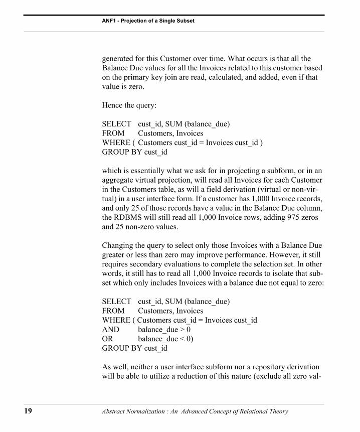
generated for this Customer over time. What occurs is that all the Balance Due values for all the Invoices related to this customer based on the primary key join are read, calculated, and added, even if that value is zero.
Hence the query:
SELECT cust_id, SUM (balance_due)FROM Customers, InvoicesWHERE ( Customers cust_id = Invoices cust_id )GROUP BY cust_id
which is essentially what we ask for in projecting a subform, or in an aggregate virtual projection, will read all Invoices for each Customer in the Customers table, as will a field derivation (virtual or non-vir-tual) in a user interface form. If a customer has 1,000 Invoice records, and only 25 of those records have a value in the Balance Due column, the RDBMS will still read all 1,000 Invoice rows, adding 975 zeros and 25 non-zero values.
Changing the query to select only those Invoices with a Balance Due greater or less than zero may improve performance. However, it still requires secondary evaluations to complete the selection set. In other words, it still has to read all 1,000 Invoice records to isolate that sub-set which only includes Invoices with a balance due not equal to zero:
SELECT cust_id, SUM (balance_due)FROM Customers, InvoicesWHERE ( Customers cust_id = Invoices cust_id AND balance_due > 0OR balance_due < 0)GROUP BY cust_id
As well, neither a user interface subform nor a repository derivation will be able to utilize a reduction of this nature (exclude all zero val-
Abstract Normalization : An Advanced Concept of Relational Theory

ues), so an exclusion of this type is only available to a query, a view, or an event utilizing an Exec SQL statement, even if it did deliver the results desired.
Through the use of an abstract, we can resolve this by the addition of a column (the ‘abstract key’) which derives its value as an abstract of an Invoice’s current ‘data-state’, and use that column to facilitate either a join, or a reference in a query.
To achieve this, we first need to determine the possible 'states' the data we want to aggregate or project can exist in this context. In this case, an Invoice is either 'Paid' or 'Open'. We then need to assign an acronym for the various data-states:
Invoice-State Indicator Paid = ’P’ Open = ’O’
We can then concatenate ’P’ for Paid and ’O’ for Open with the Cus-tomer ID (foreign key in Invoices) to create the AK (we might call the column ‘bal_due_key’, and the index ’ak_bal_due’). Therefore an Invoice which is open and which has a Customer ID assigned of 99999 would derive as ’O99999’ and one which is Paid would derive as ’P99999’ (or to better utilize index trees, ‘99999O’ and ‘99999P’) which can be enforced through form events, repository derivations, or SQL triggers. This allows us to find all open Invoices for this cus-tomer by requesting a join on ‘O99999’, rather than joining on ‘99999’ which would retrieve all Invoices regardless the state of the Invoice.
Assume this Customer has 1,000 Invoices in the Invoices table, of which 25 are ’Open’. Traditionally, as mentioned above, if we join on the Customer ID and ask for an aggregate of Invoices Balance Due, the RDBMS will have to read 1,000 rows to aggregate the Balance Due column. If instead, we join on the AK (either through a second-
Abstract Normalization : An Advanced Concept of Relational Theory 20

ANF1 - Projection of a Single Subset
21
ary AK column used to create a join in Customers, or on a variable if referenced in a query), the RDBMS will only need to read 25 rows.
These things accomplished, we can now isolate the desired subset with a single reference:
SELECT cust_id, SUM (balance_due)FROM Invoices, CustomersWHERE ( Invoices.bal_due_key = Customers.bal_due_key )
(Note that we can create the AK through either concatenation as in this case, or a Compound Index as in the example to follow.)
To reiterate, this is the root of ANF, a single index reference in the creation of an abstract, or subset, projection. The most important aspect to note is that we are now only reading a subset of the data. In other words, to expand on the benefit, assume for a moment that a Customer has a relatively constant open Invoice count of twenty-five invoices at all times. The significance here is that no matter how many closed/paid invoices this customer has in the database, whether that be 500, 1000, or 1,000,000, the performance hit for aggregating or projecting the balance due for the twenty five open invoices will be relatively constant. To be concise, there is no significant degradation in performance in maintaining this projection.
If the projection of a subset is to be in the form of a subform con-struct, or a virtual aggregate derivation in the user interface wherein Customers is the desired target table, then we’ll need to add a second-ary key to the Customers table to allow us to complete the join over the abstract key, which will default to the same data-state as the Invoices AK when an Invoice is Open. In this example, that value would be a concatenation of the data-state indicator for Open, and the Cust ID (‘O999999’). This allows us the luxury of joining the two tables via a repository relationship, or on a unique constraint, to facil-
Abstract Normalization : An Advanced Concept of Relational Theory

itate the subform projection of only those Invoices for each Customer which are Open.
We can also reverse this key, or add another column if two subform projections are desired, to project those Invoices which are Paid (‘P99999’). This can also be accomplished with a SQL view or query without the need for the creation of an additional column in Custom-ers because of our ability to state the join criteria in SQL.
Maintenance of the AK column in Invoices can occur through any one of a number of methods - a repository derivation, a trigger, or a transactional statement in a stored procedure. Since we are always maintaining this column in accordance with the Invoice’s data-state however, a back-end trigger ensures the data-correctness of this col-umn by validating and re-validating the data any time the record is touched regardless of the front end tool used.
Since all joins and query references will be ‘exact match’ joins, we can further improve performance by adding a ‘hashed index’ to this column.
The benefits of such design proliferate as uses of well defined AK’s are utilized in queries, reports, and projections, since they can be used under a number of scenarios. The above example can be used to project subforms for Open Invoices and Paid Invoices, reports for Close AR Period, Customer Statements, etc., all with the same bene-fit in performance against the same abstract key. The cost of adding the column and index is far outweighed by the benefits gained.
Example #2 -
Tables: General Ledger (GL), Journal
Abstract Normalization : An Advanced Concept of Relational Theory 22
ANF1 - Projection of a Single Subset
23
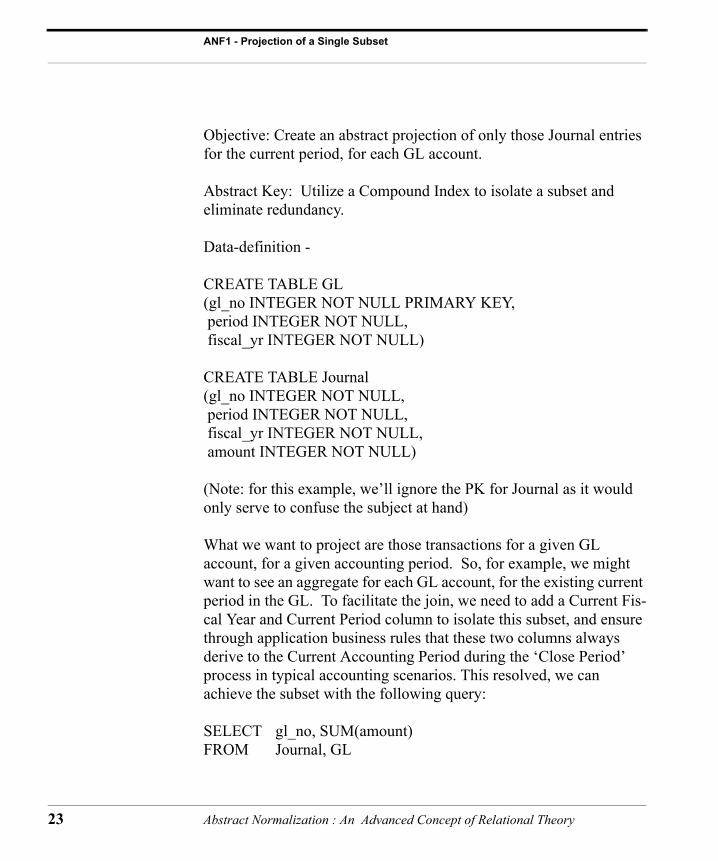
Objective: Create an abstract projection of only those Journal entries for the current period, for each GL account.
Abstract Key: Utilize a Compound Index to isolate a subset and eliminate redundancy.
Data-definition -
CREATE TABLE GL(gl_no INTEGER NOT NULL PRIMARY KEY, period INTEGER NOT NULL, fiscal_yr INTEGER NOT NULL)
CREATE TABLE Journal(gl_no INTEGER NOT NULL, period INTEGER NOT NULL, fiscal_yr INTEGER NOT NULL, amount INTEGER NOT NULL)
(Note: for this example, we’ll ignore the PK for Journal as it would only serve to confuse the subject at hand)
What we want to project are those transactions for a given GL account, for a given accounting period. So, for example, we might want to see an aggregate for each GL account, for the existing current period in the GL. To facilitate the join, we need to add a Current Fis-cal Year and Current Period column to isolate this subset, and ensure through application business rules that these two columns always derive to the Current Accounting Period during the ‘Close Period’ process in typical accounting scenarios. This resolved, we can achieve the subset with the following query:
SELECT gl_no, SUM(amount)FROM Journal, GL
Abstract Normalization : An Advanced Concept of Relational Theory
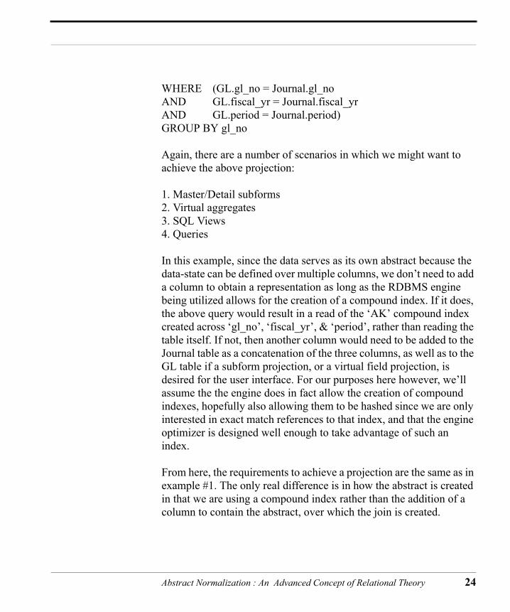
WHERE (GL.gl_no = Journal.gl_noAND GL.fiscal_yr = Journal.fiscal_yrAND GL.period = Journal.period)GROUP BY gl_no
Again, there are a number of scenarios in which we might want to achieve the above projection:
1. Master/Detail subforms2. Virtual aggregates3. SQL Views4. Queries
In this example, since the data serves as its own abstract because the data-state can be defined over multiple columns, we don’t need to add a column to obtain a representation as long as the RDBMS engine being utilized allows for the creation of a compound index. If it does, the above query would result in a read of the ‘AK’ compound index created across ‘gl_no’, ‘fiscal_yr’, & ‘period’, rather than reading the table itself. If not, then another column would need to be added to the Journal table as a concatenation of the three columns, as well as to the GL table if a subform projection, or a virtual field projection, is desired for the user interface. For our purposes here however, we’ll assume the the engine does in fact allow the creation of compound indexes, hopefully also allowing them to be hashed since we are only interested in exact match references to that index, and that the engine optimizer is designed well enough to take advantage of such an index.
From here, the requirements to achieve a projection are the same as in example #1. The only real difference is in how the abstract is created in that we are using a compound index rather than the addition of a column to contain the abstract, over which the join is created.
Abstract Normalization : An Advanced Concept of Relational Theory 24
ANF1 - Projection of a Single Subset
25
To project a subform of this subset, or an aggregate for the period transactions of the subset, we would define a join between these two tables on these three columns in the repository. The engine would then read the compound index in projecting a subform on the user interface, resulting in a single read of the source (Journal) joined on a target value in the GL table.
Finally, again, there is little if any performance degredation incurred based on the size of the Journal table as a whole. The performance hit is in direct proportion to the size of the sub-subsetset, not the size of the table. Therefore, assuming we have a relative constant subset for each period, for each GL account, regardless of the overall size of the entire set represented in the Journal table, we can maintain a great deal of history in the Journal table. This can exist with little concern for degredation, without the need to maintain an archive table, nor the need to populate result tables to obtain query results which may span both an active Journal table and an archive Journal table, resulting in much easier query writing.
Abstract Normalization : An Advanced Concept of Relational Theory
CHAPTER 4 ANF2 - Projection of Multiple Subsets
ANF2 exists across many tables to create a tertiary subset which spans those tables. The purpose of ANF2 is to create a subset projec-tion which is functionally dependent on other subsets, or perhaps, a subset of many subsets, which are projections of ANF1 constructs.
The number of applications of ANF2 is narrower than those of ANF1, and is for the most part limited to aggregations and references to those aggregations. However, the construct brings further normal-ization in the projection of subsets in an application, resulting in real-time tangible benefits to both the user and the developer.
To elaborate, we’ll be using an Inventory example which has been in use for well over five years in a variety of environments. While this is actually quite direct and simple once understood, there are several aspects which need to be reviewed to fully appreciate the impact.
The basic structure and concept is the same as in ANF1, and in both cases we can use the subset retrieved in views, master/detail situa-tions, and in queries, albeit somewhat differently. Remember that
Abstract Normalization : An Advanced Concept of Relational Theory 26

ANF2 - Projection of Multiple Subsets
27
repositories allow the use of virtual columns, front ends utilize virtual fields within a form, and SQL allows virtuals in a view. Each projec-tion has its purpose and application.
What we want to achieve in this example is to identify real-time Inventory quantities for outstanding commitments, and a real-time Inventory Quantity Available value for each Inventory Item. Our model allows us to accomplish this goal with little or no transactional code.
The tables involved are:• Inventory - target table.• OrderDetail - source table.• PODetail - source table.
In our example here, the Inventory table is the target table and the one side of the relationship, and to some extent exists as a virtual table on the front-end and in the repository (if a three-tier product is used), because the majority of the values seen are actually virtual projec-tions.
It is worthy to note that the same results can be had without the use of virtual projections by forcing a column to update through the use of triggers or procedures while still taking advantage of the abstract con-struct. However, the availability of virtual attributes at the first or sec-ond tier adds valuable benefits. This can be achieved in SQL without the benefit of either a middle-tier or a front-end through the use of views. It is also possible in some products to reduce the code required in maintaining the abstract keys though ‘cascade updates’ which is otherwise enforced through derivations, triggers, or stored proce-dures. If the RDBMS allows for a ‘cascade update’ to a foreign key, whether defined over a primary key or a unique constraint, then nei-ther a derivation, trigger, or stored procedure may be required. Unfor-tunately, not many engines come equipped with this option.
Abstract Normalization : An Advanced Concept of Relational Theory

Again, because ANF2 is an extension of, and functionally dependent on ANF1, we need to identify the various ‘data-states’ in which a record can exist to create the ANF1 constructs. This is best deter-mined by evaluating what we want to see on screen, and what we need to determine as the end result whether seen or not. In the Inven-tory table itself, we might have the following columns to identify the potential 'states' an Inventory Item can exist in. All the following states except the first one are maintained via an abstract construct using a virtual projection.
1. Physical Inventory - uncommitted, on the shelf, not maintained by an abstract. This is the only column which will most likely be main-tained transactionally, although it is possible to maintain it as a virtual projection. When an Order or Purchase Order is posted, the Physical Quantity gets adjusted transactionally and is accounted for only at the time an Order, Purchase Order, or Work Order in a manufacturing environment, is closed.
2. Customer Orders - represents open, unfilled Orders placed for Cus-tomers by the Order Entry desk (ANF1).
3. Staged Orders - represents open, un-delivered Orders, packaged and ready for delivery (ANF1).
4. Purchase Orders - represents items on order, not yet received (ANF1).
5. Received - Purchase Order Items which have been received, but not posted (ANF1).
We may also track 'Raw Materials' and 'Work In Process' using the same logic in a Manufacturing environment, but the above ‘data-states’ will suffice for our example.
Abstract Normalization : An Advanced Concept of Relational Theory 28

ANF2 - Projection of Multiple Subsets
29
It’s also worth noting that in some systems, the data-state will be determined in the master table (i.e. - Orders, or PurchaseOrders in this case), and in other systems the data-state will exist for each detail record independently (i.e. - line items for OrderDetail and PODetail), and finally in others they may exist in combination. This is because a company’s business rules may state that an Order is never closed per se, but an individual Line Item is considered closed once all quanti-ties for that item have been delivered or received. A combination can exist when an Order or PO allows for back-orders, but once the Order/PO is posted, the entire transaction is closed. For our example here, we will assume that each line item is represented independently so we don’t get lost in functional dependencies on the master table.
Data Definition Language (DDL)
CREATE TABLE Inventory(item VARCHAR (15) NOT NULL PRIMARY KEY, qty_available INTEGER NOT NULL, status_cl_key VARCHAR (16) NOT NULL, status_op_key VARCHAR (16) NOT NULL)
Note: if using SQL, add a trigger to the table to concatenate the data-states of the key values:
status_cl_key = concat (‘C’, item)status_op_key = concat (‘O’, item)
CREATE TABLE OrderDetail(item VARCHAR (15) NOT NULL, quantity INTEGER NOT NULL, status VARCHAR (1) NOT NULL, status_key VARCHAR (16) NOT NULL)
Abstract Normalization : An Advanced Concept of Relational Theory

Note: if using SQL, add a trigger to the table to concatenate the data-state of the key value:
status_key = concat (status, item)
CREATE TABLE PODetail(item VARCHAR (15) NOT NULL, quantity INTEGER NOT NULL, status VARCHAR (1) NOT NULL, status_key VARCHAR (16) NOT NULL)
Note: if using SQL, add a trigger to the table to concatenate the data-state of the key value:
status_key = concat (status, item)
The natural joins are as follows:
OrderDetail.item references Inventory.item PODetail.item references Inventory.item
To restate: the projections can be virtual columns in the repository (three-tier) or virtual fields in the front-end user interface. Depending on the application, a SQL View may well suffice for all the same rea-sons.
The virtual columns/fields we can utilize in this example are:
• Open Customer Orders (‘open’)• Staged Customer Orders (‘staged’)• Purchase Orders (‘po_open’)• PO Items Received (‘received’)• Quantity Available (‘available’)• Inventory Position (‘position’)
Abstract Normalization : An Advanced Concept of Relational Theory 30
ANF2 - Projection of Multiple Subsets
31
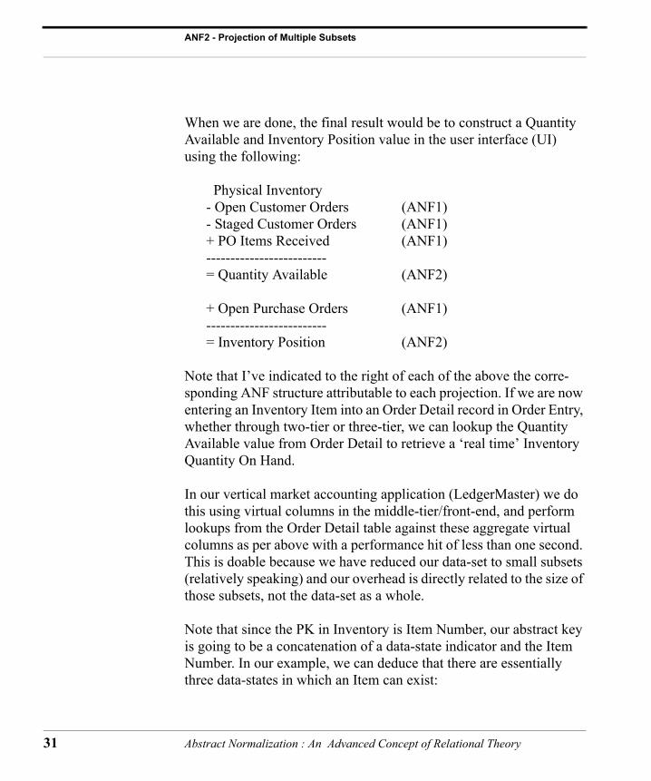
When we are done, the final result would be to construct a Quantity Available and Inventory Position value in the user interface (UI) using the following:
Physical Inventory - Open Customer Orders (ANF1) - Staged Customer Orders (ANF1) + PO Items Received (ANF1) ------------------------- = Quantity Available (ANF2)
+ Open Purchase Orders (ANF1) ------------------------- = Inventory Position (ANF2)
Note that I’ve indicated to the right of each of the above the corre-sponding ANF structure attributable to each projection. If we are now entering an Inventory Item into an Order Detail record in Order Entry, whether through two-tier or three-tier, we can lookup the Quantity Available value from Order Detail to retrieve a ‘real time’ Inventory Quantity On Hand. In our vertical market accounting application (LedgerMaster) we do this using virtual columns in the middle-tier/front-end, and perform lookups from the Order Detail table against these aggregate virtual columns as per above with a performance hit of less than one second. This is doable because we have reduced our data-set to small subsets (relatively speaking) and our overhead is directly related to the size of those subsets, not the data-set as a whole.
Note that since the PK in Inventory is Item Number, our abstract key is going to be a concatenation of a data-state indicator and the Item Number. In our example, we can deduce that there are essentially three data-states in which an Item can exist:
Abstract Normalization : An Advanced Concept of Relational Theory
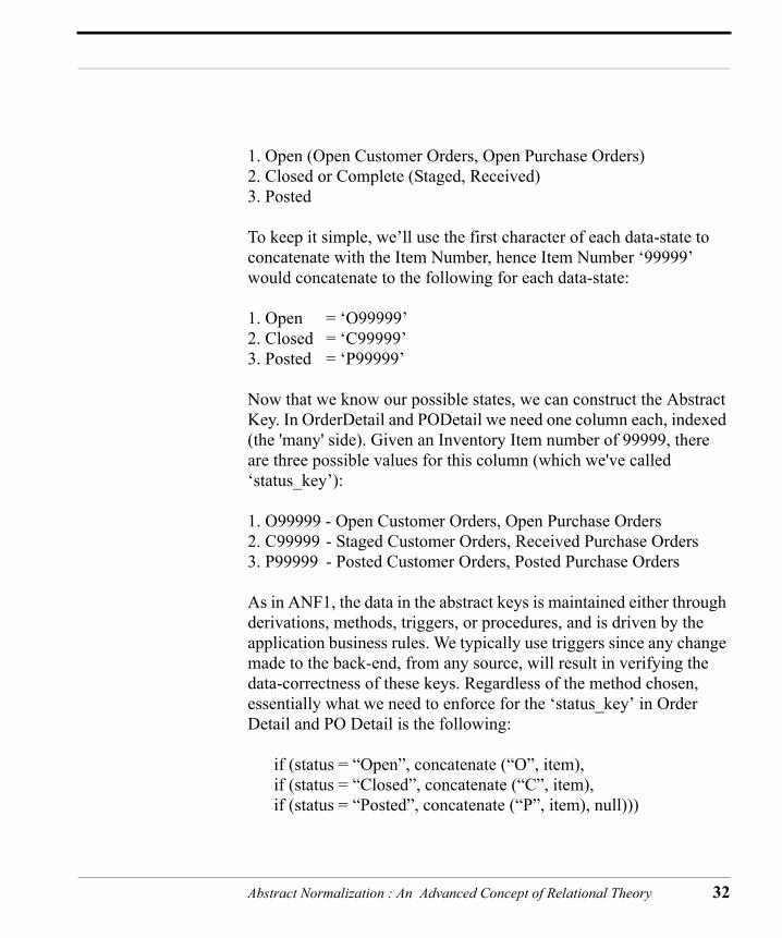
1. Open (Open Customer Orders, Open Purchase Orders)2. Closed or Complete (Staged, Received)3. Posted
To keep it simple, we’ll use the first character of each data-state to concatenate with the Item Number, hence Item Number ‘99999’ would concatenate to the following for each data-state:
1. Open = ‘O99999’2. Closed = ‘C99999’3. Posted = ‘P99999’
Now that we know our possible states, we can construct the Abstract Key. In OrderDetail and PODetail we need one column each, indexed (the 'many' side). Given an Inventory Item number of 99999, there are three possible values for this column (which we've called ‘status_key’):
1. O99999 - Open Customer Orders, Open Purchase Orders2. C99999 - Staged Customer Orders, Received Purchase Orders3. P99999 - Posted Customer Orders, Posted Purchase Orders
As in ANF1, the data in the abstract keys is maintained either through derivations, methods, triggers, or procedures, and is driven by the application business rules. We typically use triggers since any change made to the back-end, from any source, will result in verifying the data-correctness of these keys. Regardless of the method chosen, essentially what we need to enforce for the ‘status_key’ in Order Detail and PO Detail is the following:
if (status = “Open”, concatenate (“O”, item), if (status = “Closed”, concatenate (“C”, item),
if (status = “Posted”, concatenate (“P”, item), null)))
Abstract Normalization : An Advanced Concept of Relational Theory 32

ANF2 - Projection of Multiple Subsets
33
Note: if you’re doing this in SQL, use a trigger on the table to enforce the logic through a simple concatenation for both Order Detail and PO Detail tables.
In this example, we are using a column (‘status’) to determine a line item’s data-state. In actual practice, that determination usually derives from the application or company business rules based on any one of a number of factors relating to a particular line item.
Since we are going to aggregate values based on these columns from within the Inventory table for this example, we need to create a (non-indexed) column for each of these possible data-state values in Inven-tory to facilitate the abstract joins. This is only true for the target table (the 'one' side). The reason these columns do not need to be indexed is because we never have need to use a join from the source tables back to the target table since only the source tables represent the sub-set.
Hence, we created two columns in Inventory which always default to one value, a concatenation of each identified data-state and the Item Number:
1. O99999 - named "status_op_key"2. C99999 - named "status_cl_key"
The source tables always contain only one column/key to identify a subset. The reason for this is that the data value for the data-state on the many side, or source table, changes each time the data-state changes. The reason we need static representations on the target table (IE-Inventory) is to facilitate a join for each possible data-state.
This done, we can now create three joins between Inventory and the source tables:
Abstract Normalization : An Advanced Concept of Relational Theory
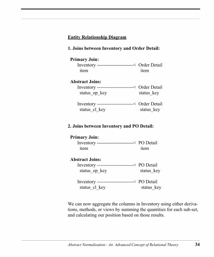
Entity Relationship Diagram
1. Joins between Inventory and Order Detail:
Primary Join: Inventory -----------------------< Order Detail item item
Abstract Joins: Inventory -----------------------< Order Detail status_op_key status_key Inventory -----------------------< Order Detail status_cl_key status_key
2. Joins between Inventory and PO Detail:
Primary Join: Inventory -----------------------< PO Detail
item item
Abstract Joins: Inventory -----------------------< PO Detail status_op_key status_key Inventory -----------------------< PO Detail status_cl_key status_key
We can now aggregate the columns in Inventory using either deriva-tions, methods, or views by summing the quantities for each sub-set, and calculating our position based on those results.
Abstract Normalization : An Advanced Concept of Relational Theory 34

ANF2 - Projection of Multiple Subsets
35
To help clarify, in SQL the queries used to facilitate the virtual aggre-gate projections (columns/fields) would be represented as follows:
Open Customer Orders:
SELECT SUM (quantity)FROM Inventory, OrderDetail WHERE (Inventory.status_op_key = OrderDetail.status_key)
Staged Customer Orders:
SELECT SUM (quantity)FROM Inventory, OrderDetailWHERE (Inventory.status_cl_key = OrderDetail.status_key)
Purchase Orders:
SELECT SUM (quantity)FROM Inventory, PODetailWHERE (Inventory.status_op_key = PODetail.status_key)
Received PO Items:
SELECT SUM (quantity)FROM Inventory, PODetailWHERE (Inventory.status_cl_key = PODetail.status_key)
These values derived, and since the Quantity On Hand is a real num-ber, we can calculate the Quantity Available:
Quantity Available = Quantity On Hand - Open-worked - Staged
And we can calculate our Inventory Position:
Inventory Position = Quantity Available + Open Purchase Orders
Abstract Normalization : An Advanced Concept of Relational Theory
Note that we use virtual columns in the middle-ware on the Inventory table and user interface form as our preferred calculation logic, and enforce the algorithm through a derivation. We've experimented with the pros and cons of various business rules here and it seems the best all around solution because it only calculates when needed, and doesn't add any overhead during inserts or updates to any of the ‘source’ tables.
If we represent this as a SQL view, the SQL statement would be as follows:
create view "dba".vw_Inventoryas select IN1.item,IN1.qty_available, sum(OD1.quantity) as Orders, sum(OD2.quantity) as Staged, sum(PD1.quantity) as Purchased, sum(PD2.quantity) as Rcvd, (IN1.qty_available-Orders-Staged+Rcvd) as Available, (Available+Purchased) as Position from "dba".Inventory as IN1, "dba".OrderDetail as OD1, "dba".OrderDetail as OD2, "dba".PODetail as PD1, "dba".PODetail as PD2 where(IN1.status_op_key=OD1.status_key) and (IN1.status_cl_key=OD2.status_key) and (IN1.status_op_key=PD1.status_key) and (IN1.status_cl_key=PD2.status_key) group by IN1.item,IN1.qty_available
What occurs is that in Order Detail, when the Item Status value changes from "O99999 to "C99999", the join is broken for Open Cus-tomer Orders, but is engaged for Staged Customer Orders.
Abstract Normalization : An Advanced Concept of Relational Theory 36

ANF2 - Projection of Multiple Subsets
37
Hence when you ask for ‘sum of <“Open” relationship> Quantity’, this row isn't even seen by the relationship because it no longer matches the ‘status_op_key’ column in Inventory. Therefore it is not aggregated, or even read. Only those rows with the value "O99999" are seen and read by the join. On the other hand, now that the ‘status’ key has changed to “C99999”, it’s picked up by the ‘Staged’ column because it now matches the value of the ‘status_cl_key’ column in Inventory (also “C99999”).
If you’ve set this up using front end virtual projections, or a view as referred to above, enter a Quantity of 100 in OrderDetail and set the Status to “O” for Open, then go to Inventory and notice that this amount will appear under that Inventory Item in the Open Customer Orders field.
Now go back to OrderDetail and change the Status to “C” for Closed, then return to Inventory if this was constructed as an application, or re-run the Inventory view above if using ISQL, and observe that the Open Customer Orders column has changed to zero, and the Staged column now reflects a quantity of 100. Notice also that when the Sta-tus is changed, the ‘status_key’ changes from “O99999” to “C99999”. Note that the change in value reflects the change in the join, and that the change in Customer Open Orders to zero occurs not because we subtracted anything, but because we are excluding the row entirely from the aggregation. Hence, there is no redundancy.
Finally, change the Order Detail Status to “P” for Posted. Notice the ‘status_key’ changes to “P99999”. If the Inventory Quantity On Hand column was driven by an abstract construct, this event would decrease the value in that column by 100. However, as mentioned above, we usually handle the physical quantity transactionally when an Order is posted. Hence, we would subtract 100 from the Quantity On Hand value procedurally.
Abstract Normalization : An Advanced Concept of Relational Theory
Some of the benefits derived are:
1. No transactional code is required to maintain any of the aggregate columns (Open Customer Orders, Staged Orders, Received, Quantity Available, etc.).
2. In the event of a system crash during a posting procedure, all aggregates and their functionally dependent (FD) columns will still be data-correct. If we were updating the Inventory aggregates using transactional means, we'd have to run an aggregate cleanup to obtain an accurate Quantity Available value.
3. It overcomes the need to account for every possible addition/sub-traction from either an aggregate column in Inventory or one of it's functionally dependent columns (Quantity Available) when inserting/updating/deleting rows in any of the 'source' tables. This is multiplied considerably when the full Inventory feature set and all the function-ally dependent columns are taken into account and we begin to account for:
• Just In Time• Turnings/Earnings• Short Percentages• Period Sold Quantities• Reorder Quantities• Economic Reorder Quantities• Reorder Points• Maximum Inventory which is even more significant when considering that:
• Work In Process• Raw Materials Committed
Abstract Normalization : An Advanced Concept of Relational Theory 38
ANF2 - Projection of Multiple Subsets
39
can also be accounted for using these same constructs.
All these constructs are maintained through an abstract, or are func-tionally dependent on an abstract derived column. Once understood and applied, the amount of transactional code which can be elimi-nated becomes significant. Everything considered, the abstracts used against this Inventory example alone result in an overall conservative reduction of some 4-5,000 lines of code in our application as a whole. If the abstract keys are correct in the source tables, and the data and indexes aren't corrupt, then all functionally dependent constructs in Inventory are correct. No guessing, no clean-up procedures, and no test procedures are needed to ensure the aggregate data is correct.
In our experience, the Inventory example has been in place since '93 in many enterprise locations with no degradation in performance due to increased data size, and has never been data-incorrect as long as the underlying source data is correct, simply because the values are maintained relationally versus transactionally.
To clarify the above, to maintain the values “relationally” means that the logic is enforced through the power of a join by way of a deriva-tion, view, subform, or any other virtual relational projection.
To enforce the values “transactionally” means that the logic is enforced through procedural code, usually to update non-virtual pro-jections.
It’s somewhat redundant, but to explain further, if we didn't use abstracts to track the various subsets representing committed and pending inventory, we'd have to trace every incident wherein a given subset is affected and add transactional code to the insert/update/delete process to affect the value of that subset in Inventory. Using abstracts, we rarely need any transactional code to maintain the con-struct. The only time it's needed is if we create an electronic trail (i.e.
Abstract Normalization : An Advanced Concept of Relational Theory

paper trail) of back-orders for example, and actually enter a new Order for the back-ordered items. In this case, we might need to ensure the key has derived correctly for the new Order since some engines might not force a recalculation at the derivation level in a batch insert, especially if there's a functionally dependent reference to a Master table. Worse case, our focus is simply on the data-correct-ness of the underlying table. The abstract will take care of the value of the aggregate projection automatically (or relationally) if the abstract key is data-correct.
As an example, if we were maintaining each category transactionally, when a Customer Order is placed, we'd have to increment the Open Customer Order column in Inventory. If an order is voided, we'd have to check for its status, and if it’s still at the Open Order stage, we have to decrement this value. If an Order is modified, we'd again have to check its status, and either increment or decrement this value. As well, we'd have to trace for any indirect modifications to Orders which may affect this value from other procedures. Every time we wrote a procedure which affected either Inventory or Customer Orders, we'd have to review and be aware of any impact our code may have on this value (as well as 'Staged'). Using an abstract, we don't care... it doesn't matter. As long as the state of the Order Detail record is correct, then the abstract key will automatically be correct because it is functionally dependent on the state. Hence, we could affect changes to the Order from any number of procedures, and never have to touch the Open Customer Order column in Inventory transactionally. It would simply derive to the correct value because of the abstract construct. Multiply this across all the subsets represented in the Inventory table and the difference in complexity, amount of code, and potential for programmer error declines considerably.
Abstract Normalization : An Advanced Concept of Relational Theory 40
ANF2 - Projection of Multiple Subsets
41
Abstract Normalization : An Advanced Concept of Relational Theory
CHAPTER 5 ANF3 - Projection of Subsets from a Set
ANF3 deals with whole tables as subsets and resolves the redundancy required to maintain Non-First Normal Form (NFNF) structures at the first level. ANF4 is an extension to ANF3 and resolves NFNF structures beyond the first level. There are some front-end require-ments to enhance the method, but the ERD remains the same regard-less.
Until this point, most of the explorations into the various levels of abstracts had centered around secondary, tertiary, and foreign keys as they relate or 'join' one table to another. However, an ongoing issue came to the forefront which necessitated an approach to solve a prob-lem which exists in many applications wherein a quasi-NFNF con-struct exists in an inefficient (non-normalized) form, whether recognized or not. This scenario is recognizable by most application programmers as redundant name/address constructs.
Before we get to the issues surrounding the abstract keys required in ANF3, lets expand on it by further exploring the issue at hand from a broader perspective.
Abstract Normalization : An Advanced Concept of Relational Theory 42

ANF3 - Projection of Subsets from a Set
43
In many applications, we find several tables which are really attributes of Names, whether they be People or Organizations. Admittedly, Names are atomically separated into Organizations and People, however the business rules for most Organizations are such that the unique attribute is actually a combination of both the Organi-zation and a Person. Ultimately, we can construct this in a number of different ways. However, even if we break Names down into Organi-zations and People (abstracts of Names, or perhaps more appropri-ately it would be named Entities, but we'll use "Names" for this example), the reality is that an Organization as well as a Name can exist as a Customer, Vendor, Shipper, etc. granting Names the privi-lege of being at the top of the heap. i.e.:
Names / \
Organizations People
Some examples of these abstract (subset) tables are:
• Customers• Vendors• Prospects• Shippers• ShipTo's• Buyers• Sellers• Members• Subscribers• Dealers
Abstract Normalization : An Advanced Concept of Relational Theory

It’s important to note that all these are really attributes of Names since each is made up of the same attributes both at a data level as well as a meta-data level. Whether these exist in a single table or not is irrelevant in the higher aspect because at an abstract level the table Names exists either in form or as an extrapolation.
One of the benefits of using NFNF constructs is the elimination of null value (or blank) columns because each NFNF construct only contains those columns which are functionally dependent on that sub-set table. For example, Customers has column requirements not needed in Vendors, and vice versa. If we didn't employ a NFNF struc-ture, then a Names record which existed as a Customer, but not as a Vendor, would leave the Vendor information columns blank, and we'd have a large number of null columns, increasing for each NFNF sub-set we might try to include in the single table.
The problem occurs when an entity record (such as a company, orga-nization, or person) exists across many tables. Probably the biggest complaint comes in the form of "address management" when an entity moves or in some way alters a record attribute such as a change in address or phone number. For every change made, every table where the entity exists has to be updated. Since each table most likely has its own unique (primary) key which is unique to that table, there is no effective way to resolve this one issue without modifying the underlying structure.
As well, even when a virtual projection is used to create a similar construct to the one we are creating here (we’ll be using a subform master/detail with a 1:1 projection to allow us to edit/enter Names from any of the sub-set tables, which a virtual projection doesn’t allow) the biggest complaint from users is that they may not have access to the parent Names table, or that they have to jump through hoops to maintain the data.
Abstract Normalization : An Advanced Concept of Relational Theory 44

ANF3 - Projection of Subsets from a Set
45
A more significant problem occurs when an entity exists in more than one of the subsets. For example, the entity may be both a Customer and a Vendor. In Customers the entity has one unique ID, while in Vendors they have another. In a standard construct, if we want to compile a report showing "Total Business Transacted" by an entity, we would need to identify each Unique ID assigned to the entity for each table we're querying. If, on the other hand, each entity (Name) had one single, unique ID, then it's simply a matter of joining this ID against all tables in question and extracting the needed data. (There's a much broader level of abstract which would allow us to delete a Name with a specific ID throughout an entire application, but it's cur-rently beyond any RDBMS ability I'm aware of. Think of the possi-bilities though.)
Given that Names contain all possible entities, we can create exten-sions, or subsets of Names.
Since a Name can also be either a Customer or Vendor, or both, the join would occur directly with the primary table:
Names/ \
Customers Vendors
Names 1:1 CustomersNames 1:1 Vendors
Notice that we also transparently end up with a 1:1 between the Cus-tomers and Vendors record for a specific Name since they have the same Primary Key.
Customers 1:1 Vendors
Abstract Normalization : An Advanced Concept of Relational Theory

This is a bit early in the discussion, but note that ShipTos are in most cases extensions of a Customer. This deviates NFNF to some degree since ShipTos are both extensions of Customers (rather than sub-sets) as well as being subsets of Names. In other words, true NFNF would dictate that the ShipTos record should also exist as a Customer. How-ever, a ShipTo may only be an attribute extension of the Customer rather than exist as a Customer. Do note however that a ShipTo can also be a Customer. This requires the ability to make a ShipTo func-tionally dependent on the Customer (constraining a list of ShipTos to a specific Customer) as well as an independent Name in their own right.
Names \
Customers\
ShipTos
Names 1:1 ShipTosCustomers 1:M ShipTos
(since ShipTos are attributes of a Customer)
This is mentioned to help elucidate the complexity of the larger issue, and to note that this can be solved within the bounds of this construct, but is solved in ANF4, which as mentioned is an extension of ANF3.
The Names record has the typical columns, though you can add/sub-tract to meet the business model needed:
name_idnameaddresscitystate
Abstract Normalization : An Advanced Concept of Relational Theory 46

ANF3 - Projection of Subsets from a Set
47
zipphone1phone2
(As a side note, to add functionality, we can also add another key “Parent ID” which will allow us to relate Names to Names to build recursive trees of related Organizations and People, which is actually an ANF1 construct. It’s fun to explore and review the possibilities, but we’ll stay focused on the construct at hand.)
We now need to create a Customers table. Essentially, this table is only going to consist of one column (that's right, one). We can add others for added functionality which is specifically applicable to a Customer, but only one column is required... and that's the Customer ID.
Then we add a relationship (join) between Customers and Names by relating the Customer ID to the Name ID. Whether this is done on the SQL back-end or in the middle ware will be dictated by your tool of choice. i.e.:
WHERE (Names.name_id = Customers.customer_id)
Now, we add a subform (master/detail) to the user interface (1:1) to Customers, which is essentially a replication in appearance to Names so that to the user there appears little difference:
customer_id nameaddresscitystatezipphone1phone2
Abstract Normalization : An Advanced Concept of Relational Theory

where everything except customer_id is a subform of Customers.
Aside from the Customer ID column, none of the columns actually belong to the Customers table, but rather, to Names. We would then add those columns which were specifically functionally dependent to the Customer ID to the table (payment_terms, customer_type, sales_person, etc.).
Here's where it gets interesting. Assuming this was created appropri-ately for your front-end of choice, you can now enter a Customer by:
1. performing a dynamic lookup (or picklist) to the Names table to first see if this Name exists, and if it does, simply highlighting the desired Name and pressing enter (or using a modal lookup form to retrieve an existing record, etc.).
2. if the Name doesn't currently exist, from here, leave the Customer ID column blank, and simply enter all the other pertinent information (Name, Address, etc.). Once complete, press Save.
If the second option is chosen, and your front end of choice is designed as such, the Customer ID should automatically be generated and a record entered in Customers. Now go to the Names table and notice that the Customer just entered exists there as well.
Now go back to Customers and modify any portion of the informa-tion. Notice the modification actually occurs in Names, even though you are working in Customers and for all intents and purposes, the user believes they are modifying the information in Customers, as well as in any of the other NFNF tables throughout the application in which this entity’s information exists. You can do the same with any NFNF table you need to add to the data-base - Vendors, Subscribers, Members, etc. - and the effect will be identical.
Abstract Normalization : An Advanced Concept of Relational Theory 48
ANF3 - Projection of Subsets from a Set
49
As an added benefit, you never have to directly allow user access to the Names table. Its inserts and updates can occur from any of the NFNF tables. The only reason for direct access to the Name table is to delete a Name, which should occur from within a procedure any-way, since all related tables will need to be checked for the entity’s existence, as well as any other business rules, such as existing tertiary records, etc., which will affect data-integrity, before being deleted.
All this said, the important point is that properly constructed, the end result to this entire construct is that we can change an entity's address (or any other direct attribute), and it will appear to cascade through all its underlying NFNF existences through the use of relational con-structs. If I change an address in a Names record, it will immediately appear as changed in all instances of that Name (Vendor, Customer, etc.). Also, I can insert or update any subset instance of a Name (in any of the related NFNF tables) and it will either create or change the data in the Names record. This is done through the use of 1:1 joins using master/detail constructs combining the power of both the front-end as well as the underlying RDBMS. This allows column mainte-nance of Name, Address, City, State, or Zip (or any other Name infor-mation) to occur from any of the NFNF tables, regardless of the number of tables involved.
To restate, from any of these tables (Customers, Vendors, Members, Subscribers, etc.), a new Name can be entered or modified, and the result is immediately reflected in the Name record, as well as across the entire database (in all affected NFNF tables).
My apologies for the redundancy in pointing out some of the benefits, but they are points well worth repeating for clarification.
The only issues which has come up from developers who have been shown and employed this construct has had to with searching and reporting. However, these are front-end issues, are easily resolvable, and beyond the scope of this treatise. I find the use of de- normaliza-
Abstract Normalization : An Advanced Concept of Relational Theory
tion to shortcut development inevitably leads to greater amounts of redundancy in fulfilling additional business requirements as they arise.
Abstract Normalization : An Advanced Concept of Relational Theory 50

ANF3 - Projection of Subsets from a Set
51
Abstract Normalization : An Advanced Concept of Relational Theory
CHAPTER 6 ANF4 - Projection of Subsets from a Subset
This is to be a short chapter since ANF4 is simply an extension of ANF3, which allows us to extend the NFNF construct as deep as needed in addition to the breadth discussed in ANF3.
To accomplish this we only need to add a second relationship to all subsets of the Names subset tables. This allows us to achieve the same benefits obtained in ANF3 for all subset subsets, as well as val-idate data-correctness within the subsets.
Assume the following:
Names\Customers
Assume we want to add a ShipTos table, which is functionally depen-dent on Customers. What we need to do is add a Customer ID column to the ShipTos table to relate it to Customers and force our pick-list to reference Customers, and at the same time add another relationship to
Abstract Normalization : An Advanced Concept of Relational Theory 52

ANF4 - Projection of Subsets from a Subset
53
relate the ShipTo ID to Name ID in Names. This second relationship allows us to create the 1:1 subform projection just as we did in ANF3 between Customers and Names, giving us the ability to add/modify attributes of the Name record from ShipTos.
From here, any deeper subset of the ShipTos table follows the same dual-relationship rules. Assume for a moment that a ShipTo record can have multiple Contacts. In that event, we would create another table as a child to ShipTos, and create a dual 1:1 relationship to Names.
This gives us:
Names \
Customers\ShipTos
\Contacts
The relationships are:
Names 1:1 CustomersNames 1:1 ShipTosNames 1:1 Contacts
Customers 1:M ShipTosShipTos 1:M Contacts
Note that even at this level, if we modify the name spelling (for example) in Contacts, we are really modifying the record in Names. In the event this entity exists anywhere else in the data-base, all changes will be reflected there as well since a Contact may also exist
Abstract Normalization : An Advanced Concept of Relational Theory

in another context within the database (i.e. - a ShipTo can also be a Customer, Vendor, etc.)
The other possible construct which follows along similar lines is when we divide up a subsets into narrower subsets, which is truer to the NFNF model than what we’ve previously discussed. Assume we have Names, then Customers, then need to separate Customers into a Male table and a Female table (separate result tables), and then need to separate Male/Female tables into Professional and BlueCollar tables, then separate these into those with Children and NoChildren... all as result tables. This can be accomplished the same way as above, except there is no need for a ParentID column since the PK column for each of these tables will be the same as the parent, which origi-nates from Names, with the abstract being the NFNF table itself.
Names |Customers/ \
Male Female / \
MProf MBlue / \
MPChild MPBNoChild
No matter how deep an NFNF structure is created, the same applies. Change the record at any level, your are really in the Names table, and they are carried to all levels.
I know, I know... smoke and mirrors of a kind. However, it has signif-icant practical applications in a number of everyday scenarios, espe-cially in Contact Management applications, and all without any transactional code. Reporting is simple and direct, with the subset identified as the table, rather than on columns in a table. Further, if a partition of the subset is desired as a permanent part of the applica-
Abstract Normalization : An Advanced Concept of Relational Theory 54

ANF4 - Projection of Subsets from a Subset
55
tion, yet another NFNF table can be created and easily populated for future reference and reporting. The applications and ramifications are simply far too numerous to expound on here, whether for reporting, picklist selection, cascading relational requirements, or for shear sim-plicity of data maintenance.
Abstract Normalization : An Advanced Concept of Relational Theory
CHAPTER 7 ANF5 - A Non-Virtual Projection from Multi-Table Joins
ANF5 delivers significant design and performance benefits to an application. It allows us to create abstract joins across many tables, and reduce redundant table constructs and the transactional code required to maintain those constructs. In a standard accounting appli-cation this results in a reduction of thousands, or even tens of thou-sands, of lines of code, as well as the elimination of several tables.
Because of its universal nature, we’ll use a typical accounting appli-cation construct for our example. We’ll first review the larger picture, then select two of the Ledger tables, along with a result table and a view to work with as an illustration.
It is important to point out for those not involved in writing or main-taining accounting systems, that the Journal table (often referred to as the “GL Subledger”) is ‘the’ central repository of information in an accounting system. From this table, we can trace back to any transac-tion in any of the primary journals, write almost all General Ledger reports, and ascertain the correctness of the data in the system as a whole. It is, in short, a rather encompassing ‘result’ table. As a point
Abstract Normalization : An Advanced Concept of Relational Theory 56

ANF5 - A Non-Virtual Projection from Multi-Table Joins
57
of interest, all the same concepts apply to an Inventory Transaction Log in an Inventory Control system, and all the same techniques can be applied that we’ll be applying to the General Ledger here.
The standard design for an accounting application encompasses four primary tables, two of which are multiplied by the number of “Led-gers” contained within the application, which for the most part differ only in their business rules. In theory, an entire accounting applica-tion can be written using these four tables, althought there are practi-cal reasons for not doing so. The four primary tables are:
1. General Ledger2. Journal (or GL Subledger)3. Ledger tables (many - AR, AP, GJ, etc.)4. Ledger detail tables (distribution tables to the Ledger table)
All accounting Ledgers write to the Journal table when a record is ‘Posted’. The Journal table data is then summarized in the General Ledger table by GL Account number and by accounting Period. We may have the following accounting Ledgers, all of which post trans-actionally to the GL Sub-ledger:
Accounts Receivable/AR DistributionsReceipts/RT Distributions Credit Memos/CM DistributionsAccounts Payable/AP DistributionsPayments/PT DistributionsDebit Memos/DM DistributionsGeneral Journal/GJ Distributions
| (Transaction Code)
|Journal table (GL Subledger)
| (Transaction Code)
Abstract Normalization : An Advanced Concept of Relational Theory

|General Ledger table
When an accounting entry is posted from anyone of these journals, typically a number of distribution entries are made in the GL Journal. The transactional code required to achieve this is significant, as is the supporting code to facilitate changes in transactions as well as ‘rebuild’ routines in the event of database corruption. Additional code is also required to summarize the Journal entries into the Gen-eral Ledger, and to maintain those values.
What ANF5 allows us to accomplish is to eliminate all the Distribu-tion tables, as well as all the transactional code required to post to the Journal table. It also provides for some real-time benefits and added flexibility to the end user.
What we end up with for structure, instead of the model above, is as follows:
Accounts Receivable (AR)Receipts (RT)Credit Memos (CM)Accounts Payable (AP)Payments (PT)Debit Memos (DM)General Journal (GJ)
|Journal (GL Subledger)
|General Ledger (GL)
Notice the lack of transactional code between these processes as well as the removal of all distribution tables.
Abstract Normalization : An Advanced Concept of Relational Theory 58

ANF5 - A Non-Virtual Projection from Multi-Table Joins
59
Unlike ANF3 or ANF4, this model is fully supportable on the back-end through the use of foreign keys, triggers, and views, and less dependent on the front-end or middle-ware for functionality.
What is rather uncommon in this structure is that all Ledger tables are master tables to Journal, with Journal being on the ‘many’ side of those relationships. This poses some interesting challenges in the middle-ware since we cannot use derivations to point to a master table (or if we do through nested ‘if’ statements, we open the door for maintenance problems each time a new accounting Ledger is added).
The data definition language (DDL) for the creation of the tables we are going to use for this example is as follows...
CREATE TABLE "GJ"( "fiscal_yr" char(4) NOT NULL,
"gj_no" char(10) NOT NULL,"journal_date"timestamp NOT NULL,"journal_note"varchar(50) NULL,"journal_ref" varchar(2) NOT NULL,"period" char(2) NOT NULL,
PRIMARY KEY (GJ_No, Journal_Ref))
CREATE TABLE "Journal"( "journal_no" char(10) NOT NULL,
"journal_note" varchar(50) NULL,"journal_ref" varchar(2) NOT NULL,"period" char(2) NOT NULL,"fiscal_yr" char(4) NOT NULL,"line_no" smallint NOT NULL,"coa_no" char(7) NOT NULL,"amount" numeric(12,2) NOT NULL,
PRIMARY KEY (journal_no, journal_ref, line_no))
Abstract Normalization : An Advanced Concept of Relational Theory
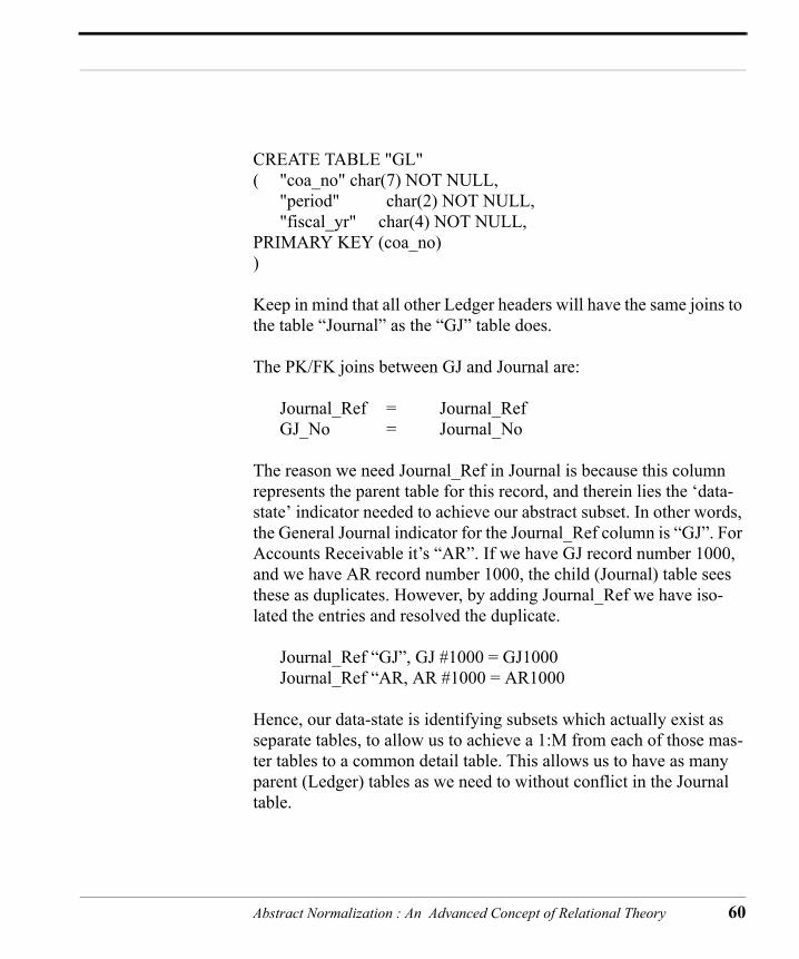
CREATE TABLE "GL"( "coa_no" char(7) NOT NULL,
"period" char(2) NOT NULL,"fiscal_yr" char(4) NOT NULL,
PRIMARY KEY (coa_no))
Keep in mind that all other Ledger headers will have the same joins to the table “Journal” as the “GJ” table does.
The PK/FK joins between GJ and Journal are:
Journal_Ref = Journal_RefGJ_No = Journal_No
The reason we need Journal_Ref in Journal is because this column represents the parent table for this record, and therein lies the ‘data-state’ indicator needed to achieve our abstract subset. In other words, the General Journal indicator for the Journal_Ref column is “GJ”. For Accounts Receivable it’s “AR”. If we have GJ record number 1000, and we have AR record number 1000, the child (Journal) table sees these as duplicates. However, by adding Journal_Ref we have iso-lated the entries and resolved the duplicate.
Journal_Ref “GJ”, GJ #1000 = GJ1000Journal_Ref “AR, AR #1000 = AR1000
Hence, our data-state is identifying subsets which actually exist as separate tables, to allow us to achieve a 1:M from each of those mas-ter tables to a common detail table. This allows us to have as many parent (Ledger) tables as we need to without conflict in the Journal table.
Abstract Normalization : An Advanced Concept of Relational Theory 60
ANF5 - A Non-Virtual Projection from Multi-Table Joins
61
Note also that we have included the GL table here to help explain some of the reasons for constructing things as they are. However, the construct in question that we want to focus on actually exists between the GJ table (and all other Ledger tables) and the Journal table. The reason we are including the GL table is because of some of the pro-jections which will be required in the GL table, whose values to accomplish those projections exist across all three tables. The PK/FK between Journal and GL is:
COA_No = COA_No
However, as mentioned above, to obtain some of the projections needed in the GL, there are also a few other ANF1 construct joins which exist using a Compound Index to obtain aggregates for the “Current Period”, “Year To Date”, and “Current Balance”. Aside from this aspect of the GL table, the theory, logic, and construct to achieve the projections in the GL table is identical to the examples in ANF1 and would be redundant to cover here, so after we’ve covered this one aspect, we’ll limit our discussion to the GJ and Journal table. We do however need to be aware of the requirements for these pro-jections because we need certain values to exist in the Journal table to achieve the above mentioned projections.
The ANF1 projections for the GL table will require the following additional joins between the Journal and the GL tables. This abstract join allows us to project an aggregate value in the GL table for those transactions which exist in an account for a specific Period/Fiscal Year:
COA_No = COA_NoPeriod = PeriodFiscal_Yr = Fiscal_Yr
Abstract Normalization : An Advanced Concept of Relational Theory
And this abstract join will allow us to project an aggregate value in the GL table for a specific account for an entire fiscal year:
COA_No = COA_NoFiscal_Yr = Fiscal_Yr
What’s important to notice from these ANF1 joins is the requirement to replicate the ‘Period’ and ‘Fiscal Year’ columns in the Journal table from the Ledger tables since these columns are functionally dependent on the Ledger tables (mostly for practical reasons). This will become clearer as we progress, but is important to note because the creation of these keys in the Journal table facilitates the abstract joins needed to create the aggregate projections in the GL table.
The PK/FK join between the GJ (and all Ledger tables) and the Jour-nal table is:
Journal_Ref = Journal_RefGJ_No = Journal_No
This join is used strictly as a PK/FK join for integrity purposes. The data-entry join includes a few other columns, and can be constructed either in the middle-tier repository, or as a unique constraint/FK con-struct. The latter (UC/FK) works fine in those SQL engines which support ‘Cascade Updates’, since any modifications to the parent table (GJ) will automatically carry through to the joined columns in the child table (Journal). The abstract join we create to achieve data-entry purposes is as follows:
Journal_Ref = Journal_RefGJ_No = Journal_NoPeriod = PeriodFiscal_Yr = Fiscal_Yr
Abstract Normalization : An Advanced Concept of Relational Theory 62
ANF5 - A Non-Virtual Projection from Multi-Table Joins
63
Note that we have added both Period and Fiscal_Yr to the abstract UC/FK join as we did in the additional joins between the Journal and the GL tables above. The reason is that because they are part of the join over which the master/detail (mainform/subform) construct is created in the user interface form, entries or changes made to these columns are automatically carried to the detail (Journal) table because they are part of the join. Otherwise, we would have to either re-enter both the Period and Fiscal Year in each line item entry in the Journal subform table, or enforce their entry through a trigger on inserts and updates. By defining the abstract across these columns, referential integrity takes care of the entries for us.
Worth reiterating, the reason for the Journal Reference column is to differentiate between differing ‘Ledger header’ table entries in the Journal table. In this example, the Journal Reference value for the GJ table will always default to “GJ” for all General Journal (GJ) entries.
So to compare the difference in logic between what we typically have in a standard construct, and what we now have in an abstract con-struct we’ll walk through a logic flow.
In a standard GJ, GJ_Distribution, Journal, and GL construct is the following:
1. The user makes their entries in the GJ table. The entries made are the GJ number, Period, Fiscal Year, and an Entry Note.
2. The user then makes entries to the GJ Distribution table, which exists as a subform to the GJ table. In this table the user enters the GL Account number, Department number, and distribution Amount.
3. Once all the entries are made (to simplify we’ll skip the audit pro-cesses here) the system posts the entries to the Journal table. The pseudo-code to post those entries would be as follows:
Abstract Normalization : An Advanced Concept of Relational Theory

INSERT INTO Journal (journal_no, coa_no, amount)SELECT gj_no, coa_no, amountFROM GJ_DistributionWHERE (posted = “N”)
We now essentially have a mirror entry of the GJ_Distribution records entered into the Journal table. In other words, we have a per-manent duplication of the data. Redundant between the GJ, GJ_Distribution, and Journal tables.
4. The system next has to transactionally post these entries up to the General Ledger to reflect accurate aggregate values.
UPDATE GLSET current_balance = current balance + amount,SET period_balance = period_balance + amountFROM JournalWHERE ( Journal.coa_no = GL.coa_noAND Journal.period = GL.periodAND Journal.fiscal_yr = GL.fiscal_yr AND posted_gl = “N” )
The entry using that method is now complete, and is by far one of the simpler posting entries compared to the transactional requirements of the other, more complex, Ledger entries (such as Accounts Receiv-able, Accounts Payable, etc.) where many entries to multiple accounts need to occur.
Contrast that with the abstract method offered through an ANF5 con-struct:
The user makes the same entries as above through the GJ entry form, but the GJ_Distribution table is eliminated and the distribution entries
Abstract Normalization : An Advanced Concept of Relational Theory 64

ANF5 - A Non-Virtual Projection from Multi-Table Joins
65
are actually made directly to the Journal table. Once the user is done they save the record and that’s it. There is no transactional code required. The entries now exist in the Journal table, and the projec-tions for the aggregates in the GL are accomplished through the ANF1 constructs mentioned above.
Further, ignoring standard accounting rules for a moment, because the Period and Fiscal_Yr are part of the abstract join, after entry, the user can go back to that record in the GJ table, change the Period and/or Fiscal_Yr, and with no reconciling transaction code, all entries and data are correct in both the Journal table, as well as the aggregates in the GL table.
We are also saved the transactional code necessary to rebuild the General Ledger and the Journal table in the event there is a system malfunction. As long as the source tables are data-correct, then all abstract projections are also correct.
Multiply these benefits across all journals in an accounting applica-tion, as well as other similar constructs, and it isn’t difficult to see the tremendous benefits gained in performance, code and table reduction, code and table maintenance, and application flexibility.
As a final comment, in the actual accounting application, we’ve added a Division and a Department to the General Ledger COA con-struct, which gives us a DivNo/CoaNo/DeptNo (1112222222333) pri-mary key. This allows for an expansion of the basic accounting model, and for multiple Divisions to exist within the same applica-tion. Each Division/Department combination can have its own Chart of Accounts, as well as its own Inventory. Many accounting systems don’t have the capacity to allow for both a Division and a Department because those systems do not utilize abstracts, or they haven’t gone to the coding expense of providing for a transactional means to achieve a tertiary join between the Ledger tables, the Ledger distribution tables, to the Journal table, and onto the GL table. By including the
Abstract Normalization : An Advanced Concept of Relational Theory

Division in the abstract, we can isolate a full set of GL Account num-bers to a specific Division and still allow for Departments within that Division. Admittedly, this serves as a secondary abstract layer for enforcing Divisional data-correctness, and tends to complicate the description of ANF5, but it serves our purpose because it also demon-strates the simplicity and power of ANF5. It also demonstrates the ability to combine abstracts in the same construct without conflict.
As you can hopefully now imagine, the possibilities are considerable.
Abstract Normalization : An Advanced Concept of Relational Theory 66

ANF5 - A Non-Virtual Projection from Multi-Table Joins
67
Abstract Normalization : An Advanced Concept of Relational Theory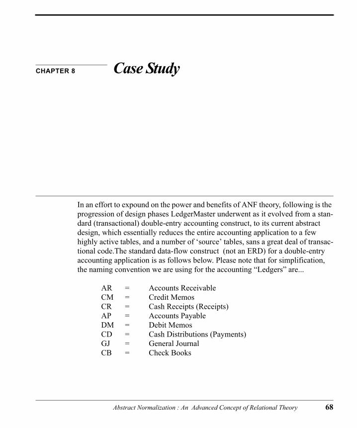
CHAPTER 8 Case Study
In an effort to expound on the power and benefits of ANF theory, following is the progression of design phases LedgerMaster underwent as it evolved from a stan-dard (transactional) double-entry accounting construct, to its current abstract design, which essentially reduces the entire accounting application to a few highly active tables, and a number of ‘source’ tables, sans a great deal of transac-tional code.The standard data-flow construct (not an ERD) for a double-entry accounting application is as follows below. Please note that for simplification, the naming convention we are using for the accounting “Ledgers” are...
AR = Accounts Receivable CM = Credit Memos CR = Cash Receipts (Receipts)
AP = Accounts PayableDM = Debit MemosCD = Cash Distributions (Payments)GJ = General JournalCB = Check Books
Abstract Normalization : An Advanced Concept of Relational Theory 68
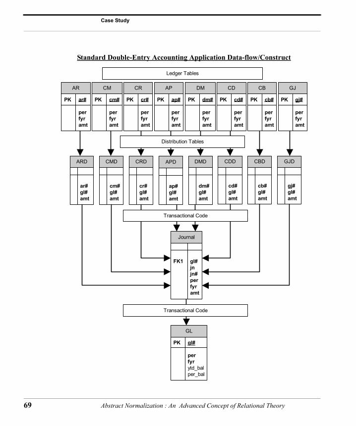
Case Study
69
Standard Double-Entry Accounting Application Data-flow/Construct
AR
PK ar#
perfyramt
CM
PK cm#
perfyramt
CR
PK cr#
perfyramt
AP
PK ap#
perfyramt
DM
PK dm#
perfyramt
CD
PK cd#
perfyramt
CB
PK cb#
perfyramt
GJ
PK gj#
perfyramt
CMD
cm#gl#amt
CRD
cr#gl#amt
APD
ap#gl#amt
DMD
dm#gl#amt
CDD
cd#gl#amt
GJD
gj#gl#amt
CBD
cb#gl#amt
Journal
FK1 gl#jnjn#perfyramt
GL
PK gl#
perfyrytd_balper_bal
Transactional Code
Transactional Code
ARD
ar#gl#amt
Distribution Tables
Ledger Tables
Abstract Normalization : An Advanced Concept of Relational Theory

Note: The ‘jn’ column in Journal represents the parent Ledger from which the transaction originated. “AR” for the AR table, etc., which allows us to perform ad-hoc joins for audit purposes, quick visual interpretations, etc.
Process flow - The user enters journal information in the respective ledger (AR, AP, etc.).
They then enter the distribution information in the corresponding dis-tribution table (ARD, APD, etc.) through a master/detail construct. This would be the GL account number (gl#) and amount to distribute (amt), the total distributions of which must equal the ledger amount in the master table.
When the entry is “posted”, the application will then transactionally post those values into the Journal table, adding a journal reference (jn) value as well as the journal number (jn#) which corresponds directly with the originating Ledger table (ie - “AR”-00001, “AP”-99999, etc.). At this point, once a period becomes ‘current’, those entries in Journal corresponding with that period are then transaction-ally aggregated into the General Ledger to obtain the YTD Balance and Period Balance used in current period financials.
In most accounting applications, when a given period is closed, the entries in the Journal are either deleted for that period, or archived to another table (xJournal), and the aggregates from that period are stored in yet another table (xGL). To simplify this study, we’ll forgo some of the more extraneous issues, but note that there are peripheral transactional requirements necessary to accommodate the standard construct.
The problems with this standard design are many from a software engineering perspective -
Abstract Normalization : An Advanced Concept of Relational Theory 70

Case Study
71
1. Redundant Tables - The distribution (ARD, APD, ...) tables are redundant, not only to one another, but also to the Journal table since they all contain essentially the same information. A variation on the Non-First Normal Form construct mentioned earlier in this work. This is not necessarily true for the Ledger tables though, since each Ledger enforces a differing set of business rules specific to that led-ger. However, in the last example in this chapter, we’ll see that there are enough similarities even in the Ledger tables, that with the right front-end, we can take this one final step as a further extension of ANF5.
2. Transactional Overhead - This can be considerable, and significant. So much so that in some systems, “posting” processes are relegated to off-hours to avoid degradation to system performance for data-entry personnel. Even limited transactional processing requirements result in reduced productivity for personnel because of the wait time incurred while waiting on system processes to complete.
3. Data-Integrity - In a file-server environment where no “roll-back” capability exists, transaction processes can be interupted, resulting in data-integrity problems in one or more tables because of partially completed transactions. To overcome this in a transactional environ-ment, additional code has to be written into posting procedures to allow for a quasi-rollback capability, usually requiring additional temp-tables, etc.
4. Data-Correctness - If modifications are desired to any of the ledger information once the item has been posted, additional transactional code has to be written and maintained to accomodate each of the events desired (delete, update, etc). In other words, the application is not ‘dynamic’, nor can data-correctness be enforced by using tools available via the relational engine. Data-correctness has to be enforced transactionally, either through triggers or stored procedures.
Abstract Normalization : An Advanced Concept of Relational Theory

By changing the relational paradigm to utilize abstract keys, we were able to mod-ify the construct as per the minimal ERD that follows. The data-flow is still the same, only the method differs.
Abstract Normal Distribution Tables - Double-Entry Accounting ERD
Ledger Tables
AR
PK jn#
jnperfyramt
CR
PK jn#
jnperfyramt
CM
PK jn#
jnperfyramt
AP
PK jn#
jnperfyramt
CD
PK jn#
jnperfyramt
DM
PK jn#
jnperfyramt
GJ
PK jn#
jnperfyramt
CB
PK jn#
jnperfyramt
GL
PK gl#
perfyrper_balytd_bal
Journal
PK,FK1,FK2,FK3,FK4,FK5,FK6,FK7,FK8 jn#PK,FK1,FK2,FK3,FK4,FK5,FK6,FK7,FK8 jnPK,FK9,FK10,FK11 gl#
FK9 perFK9,FK10 fyr
amt
Abstract Normalization : An Advanced Concept of Relational Theory 72

Case Study
73
This graphic shows the true ERD for the abstract design implemented and working in several large installations, the largest being 125 con-current users in a file/server environment. There are some consider-ations here though where joins and performance are concerned. If the back-end doesn’t allow for the creation of “compound, hashed” indi-ces, then best optimization will require the use of manufactured abstract keys. Assuming the later is the case, the following keys would need to be created...
1. GL table - ytd_key = concat (gl#, fyr)per_key = concat (gl#, fyr, per)
2. Journal - jn_key = concat (jn, jn#)ytd_key = concat (gl#, fyr)per_key = concat (gl#, fyr, per)
3. Ledgers - jn_key = concat (jn, jn#)
These are all defined as “hashed” index keys since they will always be “exact match” joins. The joins then become as follows...
1. Ledger tables to Journal table join -
Ledger tables Journal jn_key = jn_key
2. GL table to Journal table joins -
GL Journal ytd_key = ytd_key
GL Journal per_key = per_key
Abstract Normalization : An Advanced Concept of Relational Theory

In the General Ledger, we are abstracting two data-sets. Year to Date totals, and Period Totals. To accomplish that, we have to define keys that identify those data-states in the source table (Journal) so that we may aggregate those values in the GL. Hence, we define ytd_key and per_key.
In Journal, we are also defining the journal data-state of each row by combining the journal identifier (jn) with the journal reference num-ber (jn#). Journal is the source table for both GL and the journal tables because we aggregate in the GL and journal tables using Jour-nal rows as our source of those aggregates to achieve ANF1 as well as ANF5 constructs.
It’s important to note that when a period is closed, the Period and Fis-cal Year values in the GL get modified, thereby changing the join to the records in the Journal table to only those records that match the new data-state, or rather, the new Period/Fiscal Year.
Note also that the GL table can now easily exist strictly as a View, grouping on ‘source table’ joins to produce desired layouts, thereby eliminating the need for yet another table (the GL table). To the user, it won’t matter.
We’ve now resolved those problems associated with the standard construct referred to in the first graphic above...
1. Redundant Distribution Tables - we’ve removed all the distribution tables (ARD, APD, etc.) as well as their redundancy to the Journal table. Not only does this save in transactional overhead between these tables, it also eliminates the possiblity of data-correctness problems between these tables since the distribution data now resides in only one table (Journal).
2. Transactional Overhead - we’ve eliminated all the transaction overhead associated with the previous construct. The only transaction
Abstract Normalization : An Advanced Concept of Relational Theory 74
Case Study
75
overhead remaining is to enforce the business rules specific to the business for which the application is designed. Much of this also depends on the feature-set of the front-end employeed in enforcing those business rules as many can be enforced via application develop-ment restrictions. We also have no need to relegate the transactional processes to run in off-hours, because they no longer exist.
3. Data-Integrity - there are no data-integrity problems associated with partially completed transactional code in either a file-server environment, or in a client-server environment, due to system failures or the inability to achieve true roll-back capability, because the distri-bution data only exists in one table (Journal).
4. Data-Correctness - the data is always correct because there is no room for data-redundancy to occur in the distribution tables any longer. We’ve also removed the aggregation to the GL table via trans-actional means, and resolved the aggregates by using either a view, or within the reports themselves, making all aggregates dynamic (or ‘virtual’).
The overall benefit and effect is difficult to quantify until experi-enced. Once setup, training, and customization is complete, Tech Support calls are few, and are for the most part relegated to requests for new features, even in a file-server environment.
Finally, assuming the front-end of choice gives us the tools necessary, we can eliminate the remaining structural redundancy between the ledger tables. Note that unlike the data-redundancy we had between the previous two examples, this focus is solely on eliminating struc-tural redundancy and allowing for a more efficient design. The bene-fits are 1) simpler reporting constructs and 2) the ability to achieve yet a higher level of normalization for the construct as a whole.
To get there, we have to take a couple of mental leaps. If we treat the Ledger tables as ‘child’ tables....
Abstract Normalization : An Advanced Concept of Relational Theory

Ledger Tables as Child Tables
AR
PK jn#
jncust#terms
CR
PK jn#
jncust#ar_refmethodpmt_refcust_chk#dep#
CM
PK jn#
jncust#ar_ref
AP
PK jn#
jnvend#vend_po#exp_dtdue_dtpayeetermscheck#
CD
PK jn#
jncheck#ap_refvoid
DM
PK jn#
jnvend#ap_ref
CB
PK jn#
jntypepayeereturnedcheck#
Ledger
PK jn#PK jn
perfyrjdatepostedpdatenote1cb#amt
Journal
PK,FK1 jn#PK,FK1 jnPK,FK2,FK3,FK4 gl#
FK2 perFK2,FK3 fyr
amt
Abstract Normalization : An Advanced Concept of Relational Theory 76
Case Study
77
...and relate these to a single Ledger table on ‘jn’ and ‘jn#’, thereby treating the Ledger table as the ‘parent’ we can delete the redundant columns that exist across all Ledger tables in the previous examples. This possibility assumes that the user interface (front-end) allows for the use of ‘child tables’ in it’s construct(s). Note that we’ve essen-tially relegated the “GJ” table to the parent ‘Ledger’ table (as there are only 7 child tables). When a user begins data-entry, the front-end then forces them into a ‘type’ of ledger entry (AR, AP, etc), or the user could just ‘choose’ the type of entry they wish to make. Once the ‘jn’ column has received an entry type (AP, AP, etc), it would ‘make visible’ the appropriate child table and related columns for that entry, and relegate the otherwise common data-entry columns to the Ledger table, thereby simplifying reporting, transactions, etc. To the user, there is little difference, though it does allow for more flexibility in designing the UI for the developer.
From here, we can make the final leap and consolidate all redundant columns across all the child tables into the Ledger table itself, and enforce relational integrity through abstract self-referencing joins. In so doing, we’ve now reduced the total construct from 18 tables to two tables, a view (the GL), and relegated the seperation of the specific ledger tables to the user interface as Forms. Again, the user notices little, if any, difference. However, the size of the database is reduced conserably, reporting is simpler, transactional code is almost non-existant as compared to the original model, and performance benefits accordingly.
In the following ERD, I’ve also included the source tables necessary to support the transaction tables to further expound on the model.
Abstract Normalization : An Advanced Concept of Relational Theory

Ledger Table Abstraction to ANF5
Ledger
PK,FK10,FK12,FK13 jnPK,FK13 jn#
rjnrjn#perfyrjdatepdateddate
FK9 cidFK10 termFK11 cb#
chk#FK12 type
refdescamtvoid
Journal
PK,FK1 jn#PK,FK1 jnPK,FK2,FK3,FK4,FK5 gl#
FK2 perFK2,FK3 fyr
amt
JTypes
PK jnPK type
Contacts
PK cid
companynameaddresscitystzip
Checkbooks
PK cb#
banklst_chk#
Terms
PK jnPK term
G/LView
Source Tables
COA
PK gl#
descFK1 typeFK1 stypeFK2 cat
CTypes
PK typePK stype
CCategories
PK cat
Ledger (jn, jn#) 1:1 Ledger (rjn, rjn#)
Abstract Normalization : An Advanced Concept of Relational Theory 78

Case Study
79
While this may appear confusing at first, know that the referential model is still intact, and that we’ve used multiple layers of abstrac-tion to achieve our end result. With that in mind, trace the above models through this model, and it will become obvious that this is indeed the case. We’ve simply removed all UI aspects from our back-end data-store, and relegated those requirements to the front-end, which will now overlay multiple ‘views’ (or rather, ‘forms’) over the data-tables. To the user, again, there is little/no difference in what they see, or how they interact with the application.
Abstract Normalization : An Advanced Concept of Relational Theory

CHAPTER 9 Data Normalization Revisited
In discussing the subject and plans for this book with peers, it was suggested that a brief review of data normalization would be in order, if only for reference purposes. This is a reprint of an article I wrote from a few years back, and is offered here as a review on the subject.
Assume we take on a project in which the following columns all exist in a single "flat file" table. Our job is first and foremost to "normal-ize" the data before we begin applying additional business rules.
The un-normalized data items on the inherited table are: Car Serial NumberCar YearCar MakeCar ModelDealership NameDealership LocationFeature1 NameFeature1 Description
Abstract Normalization : An Advanced Concept of Relational Theory 80

Data Normalization Revisited
81
Feature2 NameFeature2 DescriptionFeature3 NameFeature3 DescriptionFeature4 NameFeature4 DescriptionFeature5 NameFeature5 DescriptionFeature6 NameFeature6 Description
1. Eliminate Repeating Groups
Our first goal is to create separate tables where each set of related attributes can be defined as being owned by a separate primary key.
In this step, we are concerned with groups of information. By identi-fying and moving these groups into separate, related tables, we achieve "First Normal Form" (1NF). In the above table, a car may have many additional features, or it may not have any. Additionally, if we want to find out which Cars have a certain Feature associated with it, the search is rather awkward and cumbersome since any one of the Feature columns could contain the information we're looking for. Ultimately, we end up paging through many records, or writing a large "if-then" query. By achieving 1NF we can then simply search against one column in the Features table, defined below, to identify those Cars which match the criteria.
Abstract Normalization : An Advanced Concept of Relational Theory

FIRST NORMAL FORM
Cars table Car Serial Number --Primary KeyCar YearCar MakeCar ModelDealership NameDealership Location
Features table Feature Code--Primary KeyFeature NameFeature Description
2. Eliminate Redundant Data
In the Cars table above, if you examine the data, you'll find repeating values:
Car# Year Make Model1234 1995 Chrysler Cirrus1235 1995 Chrysler New Yorker1236 1995 Chrysler Cirrus
Besides the repeating data in the Year and Make columns, notice also the Model for Cars #1234 and #1236. We can eliminate this redun-dancy by removing these attributes to a separate table.
To accomplish this, we divide the Cars table into two tables, Cars and car models, and retain only those attributes specific to the "primary
Abstract Normalization : An Advanced Concept of Relational Theory 82

Data Normalization Revisited
83
key" in each, with the addition of "foreign keys" to achieve the rela-tional structure:
Cars Car Serial Number--Primary KeyCar Code --Foreign KeyDealership NameDealership Location
Car Models Car Code --Primary KeyCar YearCar MakeCar Model
We now have under the Car Models table:
Code Year Make Model0001 1995 Chrysler Cirrus0002 1995 Chrysler New Yorker
and in the Cars table:
Car# Code1234 00011235 00021236 0001
A small example, but nevertheless, when applied to a large data set, the results in both efficiency and size savings are significant.
We now have:
Abstract Normalization : An Advanced Concept of Relational Theory

SECOND NORMAL FORM
Cars Car Number --Primary KeyCar Code --Foriegn KeyDealership NameDealership Location
Car ModelsCar Code --Primary KeyCar YearCar MakeCar Model
FeaturesFeature Code --Primary KeyCar Number --Foriegn KeyFeature NameFeature Description
3. Eliminate Columns Which Are not Dependent On The Pri-mary Key.
Sometimes there is a vague distinction between 2NF and 3NF, in that when 2NF is achieved, 3NF is also. Take the above for example, Dealership Name and Dealership Location may or may not be data that is redundant (in accordance with 2NF) in the Cars table. If it were, in this case we would also achieve 3NF because in conforming to 2NF we would also have created a separate table for Dealerships based on "Data Redundancy". But for our purposes here, we'll assume the data is not redundant.
Abstract Normalization : An Advanced Concept of Relational Theory 84

Data Normalization Revisited
85
To achieve 3NF under these circumstances however, we need to examine the "dependency" of a column on the primary key of that table. Dealership information is not dependent on the Car, as it can and should exist as a separate data-set on it's own. Therefore, we need to remove this information to a separate table as well. We now have:
THIRD NORMAL FORM
Dealerships Dealership Code --Primary KeyDealership NameDealership Location
Cars Car Serial Number --Primary KeyCar Code --Foreign KeyDealership Code --Foreign Key
Car ModelsCar Code --Primary KeyCar YearCar MakeCar Model
FeaturesFeature Code --Primary KeyCar Serial Number --Foreign KeyFeature NameFeature Description
Abstract Normalization : An Advanced Concept of Relational Theory

In achieving both 2NF and 3NF, our primary goal is to avoid update and delete anomolies, which we have done here. Previously, had we deleted a Car, the Dealership information would have been lost as well. Now, we can delete either the Dealership information, or the information pertaining to a Car, and the related data will be unaf-fected unless we direct the database to perform otherwise.
Third Normal Form satisfies most business requirements. However, if you wish to normalize further...
4. Isolate Independent Multiple Relationships
Tables may not contain two or more 1:N or N:M relationships that are not directly related.
Now it gets a bit more abstract.
Suppose I want to add an Accessories column to Features, so for example, a car could be red (Feature) and could come with pinstrip-ing (Accessory). This violates 4NF in that these two attributes do not share a meaningful relationship. A car may be red but not have pin-striping, or it may be red and not come with chrome mMirrors. How-ever we need a way to represent this without storing these values within the same table.
Given a Features table:
Feature Code --PKCar Serial Number --FKFeature NameFeature Description
where a Feature can come with various Accessories (e.g. pinstripes, chrome mirrors), we could add another column so the table now has:
Abstract Normalization : An Advanced Concept of Relational Theory 86

Data Normalization Revisited
87
FeaturesFeature Code --PKCar Serial Number --FKFeature NameFeature DescriptionAccessory
The problem is that more than one Accessory may be available per Feature which means we would have to enter a record for every Accessory desired and duplicate the other columns. Hence we have an inherent multiple relationship between Features and Accessories. To achieve 4nf we need to seperate the multiple relationship. To accomplish this, we add another table Accessories.
Features Feature Code --PKCar Serial Number --FKFeature NameFeature Description
Accessories Accessory Code --PKCar Serial Number --FKAccessory Description
The problem here is that it may need to be normalized to 5NF because we now have 'semantically related multiple relationships' (M:M) between Accessories, Features, and Cars. This requires add-ing yet another table. Sticking to our example, an Accessory can belong to many Features, and a Feature can have many Accessories. The solution is to create an Accessory table (not related to Cars) and
Abstract Normalization : An Advanced Concept of Relational Theory

an associative table to enforce business rules tying Accessories to Features:
AccessoriesAccessory CodeAccessory Description
Features/Accessories Feature CodeAccessory Code
Cars/Features Car CodeFeature CodeAccessory Code
If properly constructed, from the Cars table, we can now select a Fea-ture (in a Master/Detail construct), which will then determine which Accessories are available for that Feature in the Cars_Features table:
CarFeature AccessoryFeature AccessoryFeature Accessory without having to actually type in a Feature Code and Description, and an Accessory Code and Description for every incidence/combi-nation.
Abstract Normalization : An Advanced Concept of Relational Theory 88
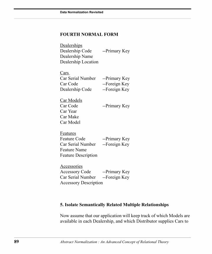
Data Normalization Revisited
89
FOURTH NORMAL FORM
DealershipsDealership Code --Primary KeyDealership NameDealership Location
Cars Car Serial Number --Primary KeyCar Code --Foreign KeyDealership Code --Foreign Key
Car ModelsCar Code --Primary KeyCar YearCar MakeCar Model
FeaturesFeature Code --Primary KeyCar Serial Number --Foreign KeyFeature NameFeature Description
AccessoriesAccessory Code --Primary Key Car Serial Number --Foreign Key Accessory Description
5. Isolate Semantically Related Multiple Relationships
Now assume that our application will keep track of which Models are available in each Dealership, and which Distributor supplies Cars to
Abstract Normalization : An Advanced Concept of Relational Theory
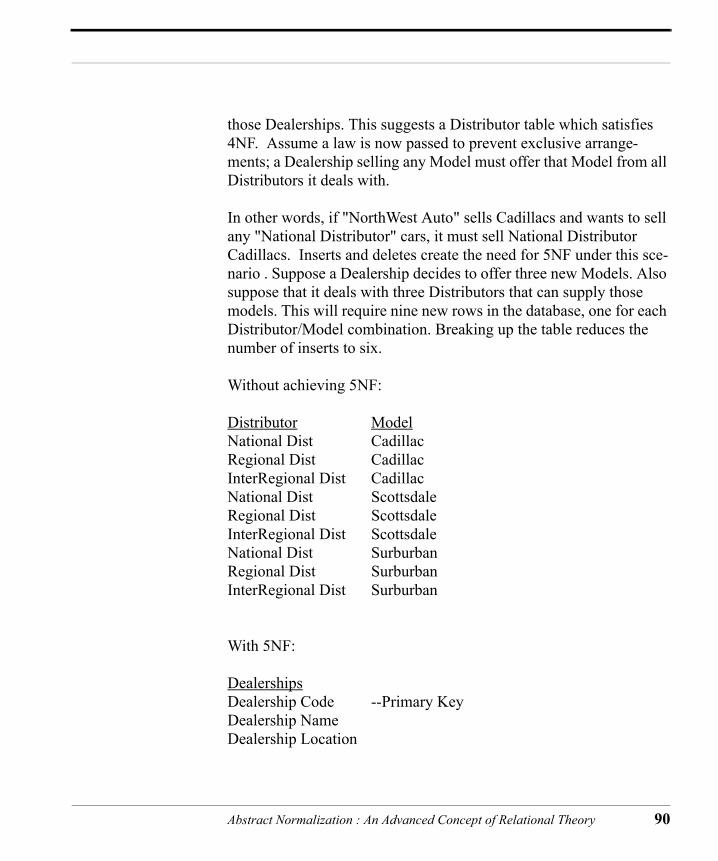
those Dealerships. This suggests a Distributor table which satisfies 4NF. Assume a law is now passed to prevent exclusive arrange-ments; a Dealership selling any Model must offer that Model from all Distributors it deals with.
In other words, if "NorthWest Auto" sells Cadillacs and wants to sell any "National Distributor" cars, it must sell National Distributor Cadillacs. Inserts and deletes create the need for 5NF under this sce-nario . Suppose a Dealership decides to offer three new Models. Also suppose that it deals with three Distributors that can supply those models. This will require nine new rows in the database, one for each Distributor/Model combination. Breaking up the table reduces the number of inserts to six.
Without achieving 5NF:
Distributor ModelNational Dist CadillacRegional Dist CadillacInterRegional Dist CadillacNational Dist ScottsdaleRegional Dist ScottsdaleInterRegional Dist ScottsdaleNational Dist SurburbanRegional Dist SurburbanInterRegional Dist Surburban
With 5NF:
Dealerships Dealership Code --Primary KeyDealership NameDealership Location
Abstract Normalization : An Advanced Concept of Relational Theory 90

Data Normalization Revisited
91
DistributorsDistributor Code --Primary KeyDistributor NameDistributor LocationDealership Code --Foreign Key
Dealerships_DistributorsDealership Code --Primary Key (join)Distributor Code --Primary Key
therefore:
Dealerships_Distributors
Dealership DistributorNorthwest Auto National DistEastWest Auto Regional DistSouthwest Auto InterRegional Dist
Dealerships_Models
Dealership ModelNorthwest Auto CadillacEastWest Auto ScottsdaleSouthwest Auto Surburban
which gives us six entries in the database versus nine entries as per above. (Obviously, we'd use Dealership Code, Distributor Code, and Model Code in the actual application instead of the names)
Abstract Normalization : An Advanced Concept of Relational Theory

FIFTH NORMAL FORM
DealershipsDealership Code --Primary KeyDealership NameDealership Location
DistributorsDistributor Code --Primary KeyDealership Code --Foreign KeyDistributor NameDistributor Location
Dealerships_DistributorsDealership Code --Primary Key (join)Distributor Code --Primary Key
Dealerships_Models Dealership Code --Primary Key (join)Car Code --Primary Key
Car ModelsCar Code --Primary KeyCar YearCar MakeCar Model
CarsCar Number --Primary KeyCar Code --Foriegn KeyDealership Code --Foreign Key
Abstract Normalization : An Advanced Concept of Relational Theory 92

Data Normalization Revisited
93
FeaturesFeature Code --Primary KeyCar Number --Foriegn KeyFeature NameFeature Description
Accessories Accessory Code --Primary Key Car Serial Number --Foreign KeyAccessory Description
The ERD (Entity Relationship Diagram) would be as follows:
DISTRIBUTORS |(1:M) |DEALERSHIPS_DISTRIBUTORS |(M:1) |DEALERSHIPS --(1:M)--DEALERSHIPS_MODELS | (M:1 relationship to CAR MODELS)(1:M) |CARS -(1:M)- CAR FEATURES | -(1:M)- ACCESSORIES(M:1) |CAR MODELS
There are other aspects to normalization, but their application is a bit more abstract. Essentially they involve the elimination of choice col-umns (moving them to user modifiable lookup tables) and the elimi-
Abstract Normalization : An Advanced Concept of Relational Theory

nation of "hard coding" variables (data-dependant) within derivations and procedures and moving those variable values to "Constants" tables (data-independent). Both are subject to opinion as to whether or not they can be classified as "Normalization" rules, but neverthe-less are quite valid in their application. Last of all, there is the need to maintain "atomic" data values in columns.
Abstract Normalization : An Advanced Concept of Relational Theory 94

Data Normalization Revisited
95
Abstract Normalization : An Advanced Concept of Relational Theory