Predictive Pre-cooling of Thermo-Active Building Systems with Low-Lift Chillers. Part II: ExperimentN.T. Gayeski, Ph.D. P.R. Armstrong, Ph.D. L.K. Norford, Ph.D.Associate Member ASHRAE Member ASHRAE Member ASHRAE

ABSTRACT This paper describes experimental results from the application of a predictive control algorithm that

optimizes control of a low-lift chiller pre-cooling a thermo-active building system in an experimental test chamber. Data-driven models of zone and concrete-core temperature response are identified from monitored test chamber temperature and thermal load data. These models are combined with an empirical model of a low-lift chiller to implement model-based predictive control. The control pre-cools a thermo-active concrete slab according to an optimal, 24-hour compressor and condenser fan speed control schedule to accomplish load shifting, part-load operation, and coolilng energy savings. Results from testing the system’s sensible cooling efficiency subjected to typical week summer conditions in two climates, Atlanta and Phoenix, show sensible cooling energy savings of 25 and 19 percent respectively relative to a high efficiency variable speed split-system air conditioner.

INTRODUCTIONThis paper describes the application of a data-driven, model-based predictive control algorithm that

pre-cools thermo-active building systems (TABS) using low-lift chillers in an experimental test chamber. The companion paper (Part I) explained the theory behind the control algorithm and reviewed the literature on control algorithms for pre-cooling thermal energy storage (TES) and controlling TABS. This paper will describe the savings measured by applying pre-cooling control to a low-lift chiller in an experimental test chamber subjected to two weekly summer climate conditions. The paper includes a description of the test chamber and the low-lift chiller, identification of data-driven temperature response models of the experimental test chamber, incorporation of these models into a predictive control algorithm, and application of the algorithm.

As described in Part I, low-lift cooling combines a variable capacity chiller operated at low pressure ratios with predictive pre-cooling of thermal energy storage (TES), such as TABS, and radiant cooling to present the chiller with lower average lift conditions and thus achieve greater cooling energy efficiency. Extensive simulation of low-lift cooling systems has shown significant potential annual cooling energy savings in a range of climates and building types (Armstrong et al 2009a, Armstrong et al 2009b, Katipamula et al 2010). For typical buildings, cooling energy savings range from 37 to 84 percent depending on the climate and building type (Katipamula et al 2010).

In this paper, the energy performance of a low-lift cooling system predictively pre-cooling TABS is compared to that of a high efficiency, variable capacity split-system air conditioner in a room-size experimental test chamber. The goal of this work is to develop the control algorithm necessary to operate a low-lift cooling system and test its performance in experiment, rather than by simulation.

EXPERIMENTAL CHAMBER AND COOLING SYSTEMAn existing experimental test facility was adapted for use in this investigation. The facility was

originally constructed in 1996 for study of conventional and displacement ventilation systems and to validate computational fluid dynamics (CFD) models. Yang (1999) and Kobayashi (2001) describe the lab facility and its material thermal properties. The lab includes two chambers, one test chamber representing a typical office zone and another chamber that can be controlled to simulate different climate conditions such as a typical summer week for Atlanta or Phoenix. A diagram of the facility is shown in Figure 1. The walls of both chambers are heavily insulated with a thermal resistance of 5.3 m2-K/W (30 ft2-F-hr/Btu). The partition between the test and climate chambers represents a typical exterior wall and contains three large

1

double pane windows which have a thermal resistance of approximately 0.27 m2-K/W (1.53 ft2-F-hr/Btu). The surrounding environment is a 20’x40’ (6m x 12m) high-bay laboratory space maintained at 20 to 24°C (68 to 75.2°F); this space can be considered to represent adjacent zones of the test room.

The climate chamber temperature is controlled by a constant volume air handling unit with an econo-mizer, pre-heating coil, cooling coil, heating coil and supply and return fans. The air handler is controlled such that the return air temperature setpoint is adjusted at every hour to follow a typical summer week of a selected typical meteorological year weather file. Fans in the climate chamber ensure that the air is well-mixed and that climate chamber air temperature, which is also recorded, closely tracks return air temperature.

Figure 1 Experimental test facility

The floor of the office chamber has been constructed to mimic a TABS system. Instead of pouring concrete over pipe, we installed a commercially available subfloor system with an aluminum top-layer and grooves into which polyethylene (PEX) pipe is inserted. Above the sub-floor, 14.6 cm (5.75 inches) of concrete pavers were installed to provide a concrete slab comparable to a TABS radiant floor. The pavers are 20.32 cm by 40.64 cm by 4.45 cm (8 in. by 16 in. by 1.75 in) blocks of concrete weighing typically 6.8 to 7 kg (15 to 15.5 lbs). By providing chilled water to the PEX pipe loop underneath the concrete pavers, the bottom of the concrete pavers, or concrete “slab”, is cooled while the top of the slab is exposed to office room, or “zone” conditions.

An air-cooled, variable capacity, low-lift chiller was installed in the climate chamber, with the condenser subjected to climate conditions. This chiller was constructed using an off-the-shelf variable capacity split-system “outdoor unit”1, described in Gayeski (2010). The seasonal energy efficiency ratio (SEER) rating of the split system is 16 Btu/Wh (4.69 Wth/We). The outdoor unit contains the compressor, condenser, condenser fan, expansion valve and electronics for the system. The conventional split-system indoor unit was installed in the test room as a base case system for comparison.

In order to chill water instead of cool air for the low-lift system, a refrigerant loop through a brazed plate heat exchanger (BPHX) was inserted across the outdoor unit suction and liquid-line ports. The BPHX is the evaporator of the low-lift chiller. It acts as a counter flow heat exchanger between the refrigerant loop and a water loop that serves the radiant concrete floor in the office chamber.

A schematic of the variable capacity chiller, its instrumentation and the climate and office test chamber piping and instruments are shown in Figure 2. The low-lift chiller is installed in the climate chamber and its condenser is subjected to controlled climate conditions. The test chamber contains the radiant concrete-core floor, the conventional “indoor unit” split-system air conditioner evaporator, and lighting and other electrical resistance heating elements to simulate typical office (Katipamula 2010) internal gains. Both systems use the same outdoor unit, and thus compressor, condenser, condenser fan, and electronic control board are identical for both low-lift and split-system modes of operation.

1 Mitsubishi MUZ-A09NA-1

2

Figure 2 Experimental test chamber and cooling system

Control over compressor speed, condenser fan speed, and electronic expansion valve position was achieved by sending serial commands from a computer through a service interface to the outdoor unit electronic control board. The compressor shaft speed can be varied from 19 to 115 Hz, the condenser fan speed from 300 to 1200 RPM, and the expansion valve position from fully closed to fully open in 400 steps. Superheat control of the expansion valve during chiller operation was achieved by tuning a PID control loop responding to the refrigerant-side temperature difference across the BPHX. A superheat control schedule was determined as a function of compressor speed for which stable superheat could be maintained. For the conventional split-system, the manufacturer’s algorithm controlled both the indoor and outdoor unit.

There are six parallel water loops in the concrete floor each made of 12.7 mm (0.5 in.) PEX pipe. These six parallel loops were designed to minimize the pressure drop through the radiant floor and reduce pumping power. The pipes are spaced 30.5 cm (12 in.) apart center to center, with the aluminum surface of the subfloor providing a conductive extended surface to thermally couple the chilled pipe to the slab. A pipe spacing of 30.5 cm (12 in.) is large for a radiant cooling system. As a result, low chilled water temperatures are required for typical cooling loads. The pipe spacing will be decreased in future work.

The chilled water pump serving the radiant floor was operated at a constant speed of 0.13 L/s (2.1 GPM) with a power consumption of approximately 145 W/L/s (9.1 W/GPM) in the installed configuration. In order to further optimize the performance of a low-lift cooling system, a variable speed chilled water pump may be used instead. However, this will increase the number of variables in the optimization and, for simplicity in this experimental implementation, the chilled water flow rate was not included as an optimization variable. For a constant chilled water flow rate, the chilled water return temperature Tchwr, the superheat setpoint for a given compressor speed, and the approach temperature of the BPHX are sufficient information to estimate refrigerant evaporating temperature Te,bphx.

The low-lift chiller is shown in Figure 3 inside the climate chamber. The condenser and condenser fan located inside the outdoor unit are at the top, the compressor wrapped in insulation is at the center, instrumentation and data acquisition equipment is at left center, the brazed plate heat exchanger is at

3

bottom center, and the chilled water loop entering the office chamber is at bottom right. Figure 4 shows the office test chamber, including the concrete radiant floor with PEX pipe loops underneath at bottom, electrical resistance heating loads enclosed in colored plastic boxes standing on the floor, the radiant chilled water loop manifold on the far right, and the conventional indoor unit finned tube evaporator mounted on the wall at top left.

These facilities were used to test the energy and thermal performance of a low-lift cooling system in which a low-lift chiller is predictively controlled to pre-cool TABS. The implementation of the control algorithm and supporting data-driven models are described in the next section, followed by a description of the experimental results.

Figure 3. Low-lift chiller located in the climate chamber

4

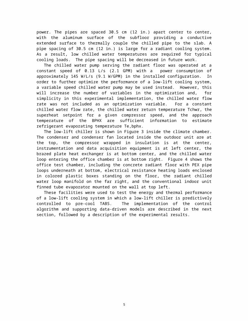
Figure 4. Test office chamber with concrete radiant floor, simulated internal loads, and a conventional split-system air conditioner indoor unit (the base case system)

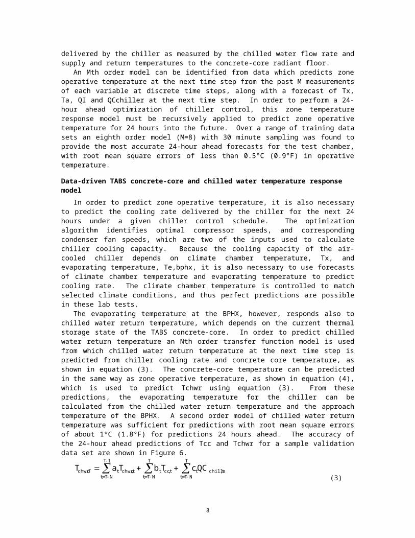
DATA-DRIVEN MODELING FOR PREDICTIVE CONTROLThe predictive control algorithm described in part 1 of this paper optimizes the compressor speed of a

low-lift chiller, such as that described above, at each hour of a 24-hour predictive control schedule. The optimization minimizes chiller power consumption, maintains thermal comfort conditions by keeping operative temperature within comfort bounds, and constrains evaporating temperature to stay above freezing. The objective function for this optimization is shown in equation (1) and is described in more detail in part 1. The first term represents energy consumption or cost, the second term is an operative temperature penalty, and the third term is an evaporating temperature penalty.

24

1ttttt PEPO1PrJminarg

(1)In order to perform this optimization, a temperature response model that predicts the zone operative

temperature as a function of forecast outdoor conditions, internal loads, and chiller control is needed. In addition, a model of chiller performance that predicts cooling rate and power consumption as a function of outdoor temperature, evaporating temperature, compressor speed and condenser fan speed is required. These data-driven models are described in more detail in the section below.

Data-driven zone operative temperature response modelComprehensive room transfer functions (CRTF) are well-established physics-based models that predict

cooling loads from zone temperatures, outdoor temperatures, and solar or internal thermal loads. (Arnmstrong et al 2006a, Seem 1987, Stephenson and Mitalas 1967, Stephenson and Mitalas 1971). Complementary to CRTFs are transfer function models from which zone temperature response can be predicted from outdoor temperature, adjacent zone temperatures, thermal loads, and the cooling rate delivered by the mechanical system, which will here be called temperature-CRTF models as shown in equation (2).

T

MTtt,chillert

T

MTttt

T

MTtt,at

T

MTtt,xt

1T

MTtt,otT,o QCqQIpToTnTmT

(2)In the temperature-CRTF model of equation (2), the temperatures and loads refer to measured

variables from sensors in the office test chamber and climate chamber shown in Figure 2. To is the operative temperature of the test chamber calculated from surface and air temperaure measurements. In a

5

conventional system, this could be replaced by a single globe thermometer measurement or other suitable measurements of comfort. Tx is the climate chamber temperature representing outdoor conditions. Ta is the temperature in an adjacent zone, in this case the lab that houses the test facility. QI is the internal heat rate to the zone delivered by light bulbs and electrical resistance heating as shown in Figure 2. QCchiller is the cooling rate delivered by the chiller as measured by the chilled water flow rate and supply and return temperatures to the concrete-core radiant floor.

An Mth order model can be identified from data which predicts zone operative temperature at the next time step from the past M measurements of each variable at discrete time steps, along with a forecast of Tx, Ta, QI and QCchiller at the next time step. In order to perform a 24-hour ahead optimization of chiller control, this zone temperature response model must be recursively applied to predict zone operative temperature for 24 hours into the future. Over a range of training data sets an eighth order model (M=8) with 30 minute sampling was found to provide the most accurate 24-hour ahead forecasts for the test chamber, with root mean square errors of less than 0.5°C (0.9°F) in operative temperature.

Data-driven TABS concrete-core and chilled water temperature response modelIn order to predict zone operative temperature, it is also necessary to predict the cooling rate delivered

by the chiller for the next 24 hours under a given chiller control schedule. The optimization algorithm identifies optimal compressor speeds, and corresponding condenser fan speeds, which are two of the inputs used to calculate chiller cooling capacity. Because the cooling capacity of the air-cooled chiller depends on climate chamber temperature, Tx, and evaporating temperature, Te,bphx, it is also necessary to use forecasts of climate chamber temperature and evaporating temperature to predict cooling rate. The climate chamber temperature is controlled to match selected climate conditions, and thus perfect predictions are possible in these lab tests.

The evaporating temperature at the BPHX, however, responds also to chilled water return temperature, which depends on the current thermal storage state of the TABS concrete-core. In order to predict chilled water return temperature an Nth order transfer function model is used from which chilled water return temperature at the next time step is predicted from chiller cooling rate and concrete core temperature, as shown in equation (3). The concrete-core temperature can be predicted in the same way as zone operative temperature, as shown in equation (4), which is used to predict Tchwr using equation (3). From these predictions, the evaporating temperature for the chiller can be calculated from the chilled water return temperature and the approach temperature of the BPHX. A second order model of chilled water return temperature was sufficient for predictions with root mean square errors of about 1°C (1.8°F) for predictions 24 hours ahead. The accuracy of the 24-hour ahead predictions of Tcc and Tchwr for a sample validation data set are shown in Figure 6.

T

NTtt,chillert

T

NTtt,cct

1T

NTtt,chwrtT,chwr QCcTbTaT

(3)

T

MTtt,chillert

T

MTttt

T

MTtt,at

T

MTtt,xt

1T

MTtt,cctT,cc QCwQIvTuTsTrT

(4)Regression from time series data can be applied to identify the coefficients of each of these models.

For practical reasons, the coefficients for the chilled water return temperature model are identified only from periods during which the chiller and chilled water pump are operating. For these experiments, the parameters of these models were estimated only once from a fixed set of training data. Alternatively, parameters could be updated continuously as new data becomes available, to account for changes in building properties over time or to continually improve the temperature response models.

Sample training data used to estimate the parameters of the models given by equations (2-4) are shown in Figure 5. The accuracy of 24 hour ahead forecasts of operative temperature, concrete-core temperature, and chilled water return temperature for a sample validation data set is shown in Figure 6. The chilled water return temperature is a discontinuous line because the chilled water pump and chiller did not operate continuously over the validation data period, and chilled water return temperature predictions are made only while the chiller is operating.

6

Figure 5. Sample temperature response model training data

Figure 6. Sample 24-hour prediction of validation data using temperature response models of test room (left) and concrete core and return water (right)

Empirical low-lift chiller performance modelModels of chiller power consumption, P, and cooling rate, QCchiller, are needed in equations (1-4) in

order to perform the predictive control optimization. Empirical curve-fit performance models of the form presented by Gayeski (2010) and repeated in equation (5) may be used. These are quad-cubic curve-fits identified by regression from detailed measurements. The models represent chiller cooling capacity or power consumption as a function of compressor speed ω, condenser fan speed f, outdoor temperature T x, and evaporating temperature Te (either Te,bphx or Te,ftc). In the low-lift predictive control algorithm, ω and f are determined by the optimization, Tx is a known forecast of climate chamber (or outdoor) temperature conditions, and Te may be predicted from past (and past predicted) values of zone operative temperature, concrete-core temperature, and chilled water return temperature using equations (2-4).

t25x24e232

2221xe20x2

19e2

18

2x17e

2x16

2e15x

2e14

313

3x12

3e11

x10e9xe82

72x6

2e54x3e21

t,chiller

fcTfcTfcfCfcTTcTcTcTcTTcTcTTccTcTc

TcTcTTccTcTccTcTccQC

(5)

7

EXPERIMENTAL ASSESSMENTThe models developed above have been incorporated into the predictive control algorithm described in

part one to test the performance of the low-lift chiller as it pre-cools the test room. The objective of these tests was to demonstrate that data-driven predictive control of chillers serving TABS could be implemented (not just in simulation) and to validate the performance of this system relative to simulated energy performance (Armstrong et al 2009a, Armstrong et al 2009b, Katipamula et al 2010).

The sensible cooling energy consumption and thermal performance of the low-lift cooling system with predictive pre-cooling of TABS was compared to that of a SEER 16 variable capacity split-system air conditioner. Two cases were studied using the typical summer week from the typical meteorological year (TMY) weather data from two climates. These two cases included a commercial office with standard efficiency internal loads subject to the Atlanta typical summer week and a commercial office with high efficiency internal loads subject to the Phoenix typical summer week. The standard and high performance loads are defined similarly to those used by Katipamula et al (2010).

The standard performance loads provided a heat rate of 36.6 W/m2 (11.6 Btu/hr-ft2) at peak load. The load schedule was 67 percent of peak load from 8:00 to 9:00 am, 100 percent from 9:00 am to 5:00 pm, and 67 percent from 5:00 pm to 6:00 pm. The high performance loads provided a heat rate of 21.5 W/m2 (6.8 Btu/hr-ft2) at peak load with a schedule of 71 percent of peak from 8:00 to 9:00 am, 100 percent from 9:00 am to 5:00 pm, and 71 percent from 5:00 pm to 6:00 pm. These loads were delivered by electrical resistance heating controlled by a programmable switch that turned loads on and off according to the defined internal load schedule. These loads are shown in Figure 2 denoted as heat rate QI measured through the heater electrical power consumption. A low velocity ceiling fan was installed in the chamber and measured as part of the internal loads to mimic the effect of a dedicated outdoor air system (DOAS) providing ventilation air and destratification.

The climate chamber air temperature, representing outdoor air conditions T x, followed the typical summer week TMY data for Atlanta, Hartsfield-Jackson airport and Phoenix, Deer Valley airport. These week-long climate chamber air temperature set points are shown in Error: Reference source not found. The other temperature input to the temperature response models, Ta in equations (2) and (4), refers to the zone adjacent to the test facility, which is the lab that houses the chamber. This temperature was kept at a fairly constant room temperature during the course of the tests. In these experiments QI, Tx, and Ta are controlled, and thus predictable inputs to the models and optimization algorithms. In practice, these variables will have error and uncertainty in prediction that must be taken into account (Henze et al 1999).

Figure 7 Typical summer week hourly outdoor air temperature (Tx) schedule for Atlanta and Phoenix

One final consideration in testing is the relative humidity of the chamber. The radiant concrete-core TABS system is intended only to provide sensible cooling, while a companion DOAS provides the latent cooling. To isolate sensible cooling effects, the relative humidity in the chamber was minimized during testing by dehumidifying zones adjacent to the test chamber, which had no internal humidity sources. A small amount of condensate water from the split system indoor unit was collected and weighed in order to deduct any latent cooling performed during operation of the base case system. This accounting was not possible for the radiant TABS system and thus any latent cooling performed by the TABS is included in its performance.

The following process was employed to evaluate performance of the low-lift cooling system and the split-system air conditioner and to compare energy consumption and thermal performance:

8

The outdoor climate chamber was continuously controlled to achieve an hourly air temperature schedule defined by a typical summer week for a selected climate as shown in Error: Reference sourcenot found.

The internal loads were programmed to followed the standard or high performance load schedule. The radiant concrete floor cooling system was operated for one week, including one weekend, after a

three day initialization period. It was programmed to maintain operative temperature between 19.5-25°C (67-78°F), based on ASHRAE (2007) during an occupied period from 8:00 am to 6:00 pm.

After completion of the low-lift cooling test, the test chamber was allowed to achieve thermal equilibrium prior to conducting split-system air conditioner tests. Particularly, concrete temperatures were allowed to return to equilibrium with the test chamber air and surface temperatures.

The split-system air conditioner was operated for one week, including one weekend, after a three day initialization period to achieve steady-periodic temperature response. The system was controlled to meet an average air temperature equal to the average operative temperature achieved by the low-lift cooling system for each corresponding day of operation. The off-the-shelf system could not be controlled to achieve operative temperature, because it operates under thermostatic control relative to its on-board air temperature sensor. However, the operative temperatures were compared after testing to ensure that a consistent level of comfort, based on daily mean operative temperature, was achieved in both cases.

ENERGY AND THERMAL PERFORMANCEFigures 8 and 9 show the results of testing the low lift cooling system and the split system air

conditioner for each case, Atlanta with standard efficiency loads and Phoenix with high efficiency loads. The figures show the operative temperature of the office test chamber and the power consumption of each system for the weekdays of the tested week. The time period begins at 6:00 pm on a Sunday and ends at the end of the occupied period, 6:00 pm, on Friday. The intial conditions for the split system and low-lift system differ because the systems were tested under steady-periodic behavior, meaning that the week prior to testing the test chamber was also conditioned by each system and allowed to achieve a steady-periodic temperature response. Thus the initial conditions, at the end of a weekend, represent those achieved by allowing the office chamber to float over the weekend after being conditioned by the system during the previous week.

A few important observations can be made from the test results. First, the low-lift cooling system runs for more hours but at lower power consumption than the split-system. It also runs in advance of the occupied period. Theses are key characteristics of low lift cooling. The cooling load is spread out over time and cooling is delivered to TABS in advance, allowing the chiller to run at lower speeds and over night when lower condensing temperatures are possible.

The operative temperature achieved by the low-lift cooling is low at the start of the occupied period and floats to a higher temperature over the course of the day as internal loads heat up the space, while the TABS system absorbs heat. This is most dramatic in the Atlanta test, in which higher density internal loads were used and oeprative temperatures rise by as much as 6°C (10.8°F) over 10 hour. This rise is below the limits for temperature variation with time suggested by ASHRAE (2007a), which allows a rise of 3.3°C (5.9°F) Celsius over four hours. However, it may well be found that a six degree rise over the day is still too much, and that a 3-4°C (5.4-7.2°F) daily rise is the limit of acceptability based on HVAC designers’ experience (Koschenz and Dorer 1999). The vertical air temperature difference within the zone was less than 1°C (1.8°F) in all cases.

The average daily mean operative temperature difference between the low-lift system tests and the split-system tests were 0.3°C (0.54°F) for the Atlanta tests and -0.5°C (0.9°F) and Phoenix tests. The low-lift cooling system conditioned the space to a slightly higher temperature on average for the Atlanta tests and a slightly lower temperature on average for the Phoenix tests. The primary difference in operative temperature is the larger daily range for the low-lift system caused by allowing zone temperatures to float.

9

Figure 8 Operative temperature and system power consumption of the low-lift cooling system and a split-system air conditioner subject to Atlanta typical summer week conditions and standard efficiency loads

Figure 9 Operative temperature and system power consumption of the low-lift cooling system and a split-system air conditioner subject to Phoenix typical summer week conditions and high efficiency loads

A comparison of the energy performance of the two systems is shown in Error: Reference source notfound1. The table shows relative performance in terms of cooling delivered, energy consumed, average coefficient of performance (COP) average energy efficiency ratio (EER), and average pressure ratio over the duration of the test. The energy consumption measurement for both systems is essentially exact. Comparing the other data requires caution primarily due to inconsistency in refrigerant flow measurement. The cooling rate could not be measured continuously during the tests because the refrigerant mass flow

10

meter cannot measure flow while two-phase flow exists. This occurs frequently during transient conditions especially under the conventional split-system air conditioner control.

Consequently, the total cooling delivered under split-system operation is underestimated and the COP and EER of the split system can be estimated in two different ways. First, the average measurable instantaneous COP from periods of stable mass flow readings may be used. This estimate ignores the actual COP in periods for which the mass flow meter could not provide a stable measurement. The second estimate can be made from the total measurable cooling delivered divided by the total energy consumed provides. The actual average COP for the split systsm during testing lies somewhere in between these two estimates. Therefore, only a range in percent improvement in COP and EER for the split-system air conditioner can be inferred, as shown in Table 1.

Table 1. Energy and thermal performance of low-lift cooling relative to a SEER 16 split system variable capacity air conditioner

Label Atlanta PhoenixSplit-system

Low-lift Difference Split-system

Low-lift Difference

Cooling (Whth)Cooling (kBtu)

-38,927 -48,002 23%a -57,199 -65,879 13%

Energy (Whe) 14,465 10,982 -25% 21,153 17,205 -19%Energy consumption (Whe)With latent cooling deducted

14,053b 10,982b -22% 21,153 17,205 -19%

Average COP 2.66-4.0 a 4.4 9-40% a 2.7-4.1 a 3.97 -3.2-32% a

Average EER 9-13.6 a 15 9-40% a 9.2-13.9 a 13.5 -3.2-32% a

Average pressure ratio 1.91 1.70 -11% 2.12 1.99 -6%a. Split-system cooling rate is under-estimated due to limitations of the refrigerant mass flow meterb. The latent energy consumption can only be estimated for split-system operation based on measurement of condensate water. The low-lift system also may have performed some latent cooling.

The results show that low-lift cooling system sensible cooling energy savings are indeed significant relative to a high efficiency split-system air conditioner. The actual measured energy consumption of the low-lift system was 25% less than the split-system under Atlanta conditions and 19% less under Phoenix conditions. Accounting for latent cooling performed by the split system, but not the low-lift system, reduces the savings to 22% for Atlanta. These results are comparable to the estimated annual cooling energy savings, 28.8%, simulated by Katipamula et al (2010) for a low-lift cooling system with ideal TES relative to a variable air volume (VAV) system with a variable speed chiller in Atlanta subject to standard efficiency internal loads. For Phoenix, the results are significantly different, 19% for the lab test relative to 42% annual cooling energy savings simulated by Katipamula et al (2010) for the same systems in Phoenix and using the high efficiency internal loads.

The differences in the basis for these two savings estimates should be carefully noted. Most importantly, the savings presented in this research are based on the measured performance of a laboratory system subject to a typical summer week rather than the simulated performance of a system over an entire year. Furthermore, the base line VAV system simulated by Katipamula et al (2010) includes an air-side economizer and higher specific fan power and the simulated low-lift system includes a refrigerant side economizer, ideal TES, and a different chiller performance map. Because of these differences, the savings described above cannot be directly compared, although they provide context for expected system savings.

The limitations of the test facility must also be recognized in interpreting the energy performance results. The chiller is somewhat oversized for the small test chamber. The internal loads were somewhat oversized in an attempt to match the chiller capacity, but this results in a mismatch between the concrete floor storage capacity, cooling capacity and the test chamber thermal loads. This mismatch inhibits the performance of the low-lift system by requiring more cooling, and allowing less load shifting than would be required for a well-matched system. In addition, the test chamber is a single story zone, where cooling energy losses from the bottom of the slab do not contribute to cooling of a space below as they would in a multi-story concrete-core system. The insulation below the concrete floor, while significant, was not enough to prevent cooling energy losses from the bottom of the slab resulting in lower thermal storage efficiency than would be achieved in a multi-story TABS. It can be seen in Table 1 that the low-lift system may provide more cooling during the test period than the split-system air conditioner because of losses

11

through the bottom of the test chamber. Furthermore, the 30.5 cm (12 in.) pitch of the radiant water pipes was, in retrospect, too large and not made up for by the aluminum facing on the subfloor. All of these factors combine to cause lower evaporating temperatures, lower thermal storage efficiencies, lower radiant floor capacities, and overall less efficient performance of the low-lift cooling system than could be achieved in a full-scale, properly sized system.

SUMMARY AND DISCUSSIONParts one and two of this paper have shown that a data-driven, model-based predictive control

algorithm can be applied to pre-cool TABS using chillers operated at low pressure ratios, called low-lift chillers, to achieve significant sensible cooling energy savings relative to a high efficiency split-system air conditioner. A low-lift cooling system was tested in a room-size laboratory test chamber. Thermal loads due to climate and internal gains were applied to the test chamber through a controlled climate chamber and scheduled electrical resistance loads installed in the test chamber. Sensors installed in the chamber were utilized to identify data-driven temperature response models of zone operative temperatuer, TABS concrete-core temperature, and chilled water return temperature. An empirical quad-cubic curve-fit model of a low-lift variable capacity chiller (Gayeski 2010a) was used to predict chiller cooling capacity and power consumption. Using these models, the data-driven model-based predictive control algorithm described in part one of this paper was applied to pre-cool the TABS installed in the test chamber using a low-lift chiller. The results of these tests show that the low-lift cooling system achieved significant sensible cooling energy savings relative to a conventional high efficiency split-system air conditioner, as shown in Table 1.

Certain improvements to the methods presented in this paper and to the laboratory test facility are likely to increase the savings that can be demonstrated using a low-lift cooling system. First, improvements to the test room such as decreased chilled water pipe pitch, additional under-slab insulation, better sizing of the chiller, and optimization of the brazed plate heat exchanger are expected to improve low-lift cooling system performance. A number of improvements to the methods presented in this paper may also enhance low-lift cooling system savings potential. Incorporating variable speed chilled water flow into the optimization algorithm will allow for better optimization of evaporating temperature relative to cooling rate and thus improved chiller efficiency. Eliminating the need to predict concrete-core temperature Tcc by predicting chilled water return temperature directly from forward modeling of the TABS has potential to reduce sensor requirements and improve the accuracy of prediction for chilled water return temperature Tchwr.

ACKNOWLEDGMENTSThe authors wish to acknowledge the Masdar Institute of Science and Technology for support of this

research. The authors are also grateful for the support and advice of members of the Mitsubishi Electric Research Laboratory and the Pacific Northwest National Laboratory. Nicholas Gayeski is also thankful for the support of the Martin Family Society of Fellows for Sustainability.

REFERENCES

Armstrong, P.R., W. Jiang, D. Winiarski, S. Katipamula, L.K. Norford, and R.A. Willingham. 2009a. Efficient low-lift cooling with radiant distribution, thermal storage, and variable-speed chiller controls – Part I: component and subsystem models. HVAC&R Research 15(2): 366-400.

Armstrong, P.R., W. Jiang, D. Winiarski, S. Katipamula, and L.K. Norford. 2009b. Efficient low-lift cooling with radiant distribution, thermal storage, and variable-speed chiller controls – Part II: Annual energy use and savings. HVAC&R Research 15(2): 402-432.

Armstrong, P.R., S.B. Leeb, and L.K. Norford, Control with building mass – Part I: thermal response model. ASHRAE Transactions Vol. 112(1)

Armstrong, P.R., S.B. Leeb, and L.K. Norford, Control with building mass – Part II: simulation. ASHRAE Transactions Vol. 112(1)

American Society for Heating, Refrigerating, and Air-Conditioning Engineers (ASHRAE). 2007. Thermal Environmental Conditions for Human Occupancy. ANSI/ASHRAE Standard 55-2007. American Society of Heating, Refrigerating, and Air-Conditioning Engineers, Atlanta, GA.

12

Braun, J.E. 1990. Reducing energy costs and peak electrical demand through optimal control of building thermal storage. ASHRAE Transactions 96(2): 876–888.

Brunello, P., M.D. Carli, M. Tonon, and R. Zecchin. 2003. Applications of heating and cooling thermal slabs for different buildings and climates. ASHRAE Transactions: Symposia 2003: 637-646.

Henze, G., R.H. Dodier, and M. Krarti. 1997. Development of a predictive optimal controller for thermal energy storage systems. Int’l. J. HVAC&R Research 3(3): 233–264.

Henze, G., and M. Krarti. 1999. The impact of forecasting uncertainty on performance of a predictive optimal controller for thermal energy storage systems. ASHRAE Transactions 105(1): 553–561.

Henze, G., C. Felsmann, and G. Knabe. 2004. Evaluation of optimal control for active and passive building thermal storage. International Journal of Thermal Sciences 43(2): 173-183.

Henze, G., C. Felsmann, D. Kalz D, and S. Herkel. 2008a. Primary energy and comfort performance of ventilation assisted thermo-active building systems in continental climates. Energy and Buildings 40: 99-111.

Gayeski, N. 2010a (submitted). Empirical modeling of a rolling-piston compressor heat pump for predictive control in low-lift cooling. ASHRAE Transactions.

Gayeski, N. 2010b. Predictive Pre-Cooling Control for Low-Lift Radiant Cooling using Building Thermal Mass. Doctor of Philosophy in Building Technology dissertation. Massachusetts Institute of Technology.

Gayeski, N. 2010c (submitted). Predictive Pre-Cooling of Thermo-Active Building Systems with Low-Lift Chillers Part 1: Control Algorithm. Int’l. J. HVAC&R Research.

Gwerder, M., Lehmann, B., Todtli, J., Dorer, V., & Renggli, F. (2008). Control of thermally-activated building systems (TABS). Applied Energy , 85, 565–581.

Katipamula S.K., P.R. Armstrong, W. Wang, N. Fernandez, H. Cho, W. Goetzler, J. Burgos, R. Radhakrishnan, and C. Ahlfeldt. 2010. Cost-Effective Integration of Efficient Low-Lift Baseload Cooling Equipment FY08 Final Report. PNNL-19114. Pacific Northwest National Laboratory. Richland, WA.

Kobayashi N. 2001. Floor-Supply Displacement Ventilation System. Masters Thesis. Massachusetts Institute of Technology.

Lehmann, B., V. Dorer, and M. Koschenz. 2007. Application range of thermally activated buildings systems tabs. Energy and Buildings 39 (2007) 593-598.

NIST. 2009. NIST Reference Fluid Thermodynamic and Transport Properties Database (REFPROP): Version 8.0. NIST Standard Reference Database 23

Seem, J.E. 1987 Modeling of heat transfer in buildings. PhD Thesis, University of Wisconsin, Madison.Stephenson, D.G., and G.P. Mitalas. 1967. Cooling load calculations by thermal response factor method.

ASHRAE Transactions 73(1)Stephenson, D.G., and G.P. Mitalas. 1971. Calculation of heat conduction transfer functions for multi-

layer slabs. ASHRAE Transactions 77(2):117–126.Todtli, J., Guntensperger, W., Gwerder, M., Haas, A., Lehmann, B., & Renggli, F. (2005). Control of

Concrete-Core Conditioning Systems. Proceedings of the 8th REHVA World Congress. Lausanne (Switzerland).

Yang X. 1999. Study of Building Material Emissions and Indoor Air Quality. PhD Thesis. Massachusetts Institute of Technology.

13