abstract interpretation meets convex optimization...
TRANSCRIPT

Abstract Interpretation Meets Convex Optimization ?
Thomas Martin Gawlitza1, Helmut Seidl2, Assale Adje3, Stephane Gaubert4, and EricGoubault5
1 CNRS/VERIMAG, France [email protected] Technische Universitat Munchen, Germany [email protected]
3 CEA, LIST and LIX, Ecole Polytechnique (MeASI) [email protected] INRIA Saclay and CMAP, Ecole Polytechnique, F-91128 Palaiseau Cedex, France
5 CEA, LIST (MeASI), F-91191 Gif-sur-Yvette Cedex, France [email protected]
Abstract. Numerical static program analyses by abstract interpretation, e.g., theproblem of inferring bounds for the values of numerical program variables, arefaced with the problem that the abstract domains often contain infinite ascend-ing chains. In oder to nevertheless enforce termination one traditionally applies awidening/narrowing approach that buys the guarantee for termination for loss ofprecision. However, recently, several interesting alternative approaches for com-puting numerical invariants by abstract interpretation were developed that aim athigher precision. One interesting research direction in this context is the studyof strategy improvement algorithms. Such algorithms are successfully applied forsolving two-players zero-sum games. In the present paper we discuss and com-pare max-strategy and min-strategy improvement algorithms that in particular canbe utilized for computing numerical invariants by abstract interpretation. Our goalis to provide the intuitions behind these approaches by focussing on a particularapplication, namely template-based numerical analysis.
1 Introduction
Mathematical optimization aims at finding a value within an area of feasible valueswhich maximizes (resp. minimizes) a given objective function. Quite efficient tech-niques have been developed for particular cases that are important in practice, e.g., whenthe objective function is linear and the area of feasible values a convex polytope (lin-ear programming, see e.g. Schrijver [21]) or even an intersection of a convex polytopewith the positive semi-definite cone (semi-definite programming, see e.g. Todd [22]) ora convex set that is defined through convex constraints (convex optimization, see e.g.Boyd and Vandenberghe [5], Nemirovski [16]). In a certain sense, also numerical staticprogram analysis based on abstract interpretation can often be cast as an optimizationproblem as follows: Assume that we are given a complete lattice of potential programinvariants at program points, i.e., an abstract domain. Then, the abstract semantics ofeach control-flow edge from a program point u to a program point v induces constraints
? This work was partially funded by the ANR project ASOPT.?? VERIMAG is a joint laboratory of CNRS, Universite Joseph Fourier and Grenoble INP.

on the invariants for u and v. These constraints describe the feasible area. The objectiveof the analysis is to minimize all invariants for the program points.
In general, it is not clear how this insight may lead to better algorithms. In this pa-per, however, we show that in case of template-based analysis of relational numericalproperties, techniques from mathematical optimization allow to construct novel pro-gram analysis algorithms. The templates we consider are (multivariate) polynomials inthe program variables such as 2x2
1 + 3x22 + 2x1x2, where x1 an x2 are program vari-
ables. The goal of the analysis is to determine, for every program point v, a safe upperbound to each template when reaching that program point v. In order to be as preciseas possible, this upper bound should be as small as possible. Different templates mayserve different purposes. If the analysis is only meant to infer (decently small) inter-vals for the values of the program variables x1, . . . , xn, templates of the form xi and−xi suffice. If the analysis additionally should infer bounds on the differences betweencertain variables, templates of the form xi − xj should be used.
Templates consisting of arbitrary linear combinations have been introduced andstudied by Sankaranarayanan et al. [19]. In some cases, e.g., when trying to prove thatcertain linear filters do not lead to floating-point overflows, linear templates are notsufficient (see e.g. Feron and Alegre [8]). However, these cases can be treated by usingquadratic templates (see e.g. Adje et al. [2], Feron and Alegre [7]).
Instead of directly performing the template based analysis, we reduce the analysisproblem to the problem of computing least solutions for systems of in-equations of theform
xi ≥ f(x1, . . . ,xn) (1)
where the unknowns of the system now may take values in R := R ∪ {−∞,∞} andthe right-hand sides f are monotone and concave operators on R. The unknowns arethe upper bounds to the templates at the different program points. For the problem ofsolving system (1), we present two strategy improvement approaches:
The Min-Strategy Iteration Approach The min-strategy iteration approach as advo-cated by Adje et al. [2] is, for the particular case we are studying in the presentpaper, similar to Newton’s method. It starts with some solution of (1) and con-structs a decreasing sequence of solutions. For any solution x, the next solution isconstructed by over-approximating each concave right-hand side f in (1) with alinear function Tf,x satisfying Tf,x(x) = f(x). The improved next solution x′ of(1) then is obtained as the least solution of the resulting linear constraint system
xi ≥ Tf,x(x1, . . . ,xn) (2)
which can be computed by means of linear programming. The crucial step hereis to determine, for a monotone and concave function f and a given vector x, thelinear function Tf,x with Tf,x(x) = f(x). If f is a point-wise minimum of finitelymany affine functions, then Tf,x can be chosen as one of the affine functions oc-curring in the minimum. In this paper, we are in particular interested in the morechallenging cases where f is not simply the point-wise minimum of finitely manyaffine functions. In the cases of interest f is defined by means of a parametrized
2

convex optimization problem. Then, Tf,x can be computed by solving a convex op-timization problem that basically consists of the duals of the parametrized convexoptimization problems. If the parametrized convex optimization problem that de-scribes f is a linear programming problem, then we can use linear programming fordetermining Tf,x. If the parametrized convex optimization problem that describesf is a semi-definite programming problem, then we can use semi-definite program-ming for determining Tf,x.
The Max-Strategy Iteration Approach The max-strategy iteration approach ofGawlitza and Seidl [13] considers the constraint system (1) as a system of equa-tions
xi = fi1(x1, . . . ,xn) ∨ . . . ∨ fimi(x1, . . . ,xn) , i = 1, . . . , n (3)
where the right-hand side of each unknown xi is the finite maximum of concavefunctions fij (here, ∨ denotes the maximum operator, i.e., x∨y = max {x, y}). Inorder to compute the least solution of (3), Gawlitza and Seidl suggest max-strategyiteration. A max-strategy can be considered as a function that selects, for each un-known xi, one monotone and concave fij from the right-hand side of xi. Gawlitzaand Seidl present an algorithm which precisely computes the least solution of (1)by iterating over max-strategies. In order to evaluate and improve a max-strategy,this algorithm requires a black box algorithm for computing greatest finite solutionsof systems of in-equations of the form xi ≤ f(x1, . . . ,xn) where f is monotoneand concave. How this black box algorithm can be realized depends on the class ofoperators the operators occurring in the right-hand sides of (1) are from.
If the operators occurring in (1) can be implemented through parametrizedlinear programs, the whole max-strategy improvement step can be implementedby linear programming. Likewise, if the operators can be implemented throughparametrized semi-definite programs, the max-strategy improvement step can beimplemented by semi-definite programming.
In the linear case, the above strategy iteration techniques can be applied to computeinvariants for template domains where all templates are linear combinations of programvariables. In the simple case of intervals, these approaches allow to perform intervalanalysis without widening [6, 11]. In case of more complex linear combinations, arbi-trary template polyhedra domains [19] such as the octagon domain [15] can be handled[9, 10]. For quadratic templates, the above strategy iteration approaches can be utilizedfor computing (resp. approximating) a semi-definite relaxation of the abstract semantics(cf. Adje et al. [2], Gawlitza and Seidl [13]).
The present paper is structured as follows: In Section 2 we discuss a simple ex-ample, where one is not able to infer non-trivial invariants through an analysis that isbased on liner templates. However, non-trivial invariants can be obtained with quadratictemplates and a semi-definite relaxation of the resulting abstract semantics. In Section3 we discuss how we should relax an abstract semantics such that the resulting relaxedsemantic equations fit in our framework, i.e., can be translated into a system of in-equations of the form x ≥ f(x1, . . . ,xn), where f is a monotone and concave operatoron R. After introducing some notations in Section 4, we explain the min-strategy ap-proach and the max-strategy approach in Sections 5 and 6, respectively. Here, we don’t
3

aim at completeness. Instead, we omit most of the things that are not directly connectedto our application. Section 7 is dedicated for a comparison of the two approaches and aconclusion.
2 Motivation and Running Example
In this subsection we are going to have a look at a small example: the harmonic os-cillator example of Adje et al. [2]. The program consists only of the following simpleloop:
f l o a t x 1 , x 2 , tmp ;x 1 = r a n ( ) ;x 2 = r a n ( ) ;whi le ( TRUE ) {
p r i n t f ( ”%f , %f \n ” , x 1 , x 2 ) ;tmp = 1 . ∗ x 1 + 0 . 0 1 ∗ x 2 ;x 2 = −0.01 ∗ x 1 + 0 . 9 9 ∗ x 2 ;x 1 = tmp ;
}
Here, we assume that ran () returns a random float value between 0 and 1, where 0 and1 are included. Figure 1 shows the control-flow graph of the program. The program
st
„x1
x2
«:=
„1 0.01
−0.01 0.99
«„x1
x2
«(x1, x2) ∈ [0, 1]× [0, 1]
Fig. 1. The Harmonic Oscillator
implements an Euler explicit scheme with a small step h = 0.01, i.e., it simulates thelinear system (
x1
x2
)←(
1 h−h 1− h
)(x1
x2
).
The invariant found with our strategy improvement methods (we are going to explainthese methods in Section 5 and Section 6) is shown in Figure 2. For finding this invari-ant, we aimed at computing upper bounds b1, . . . , b5 ∈ R = R ∪ {−∞,∞} that are
4

Fig. 1. An harmonic oscillator, its Euler integration scheme and the loop invariantfound at control point 2
x = [ 0 , 1 ] ;v : = [ 0 , 1 ] ;h = 0 . 0 1 ;whi l e ( t rue ) { [ 2 ]
w = v ;v = v!(1"h)"h!x ;x = x+h!w; [ 3 ] } {!1.8708 " x " 1.8708, !1.5275 " v " 1.5275, 2x2 + 3v2 + 2xv " 7}
these quantities. This means that we consider the linear templates based on{x,!x, v,!v}, i.e. intervals for each variable of the program, together with thenon-linear template 2x2 + 3v2 + 2xv. The last template comes from the Lya-punov function that the designer of the algorithm may have considered to provethe stability of his scheme, before it has been implemented. In view of provingthe implementation correct, one is naturally led to considering such templates1.Last but not least, it is to be noted that the loop invariant using intervals, zones,octagons or even polyhedra (hence with any linear template) is the very disap-pointing invariant h = 0.01 (the variables v and x cannot be bounded.) However,the main interest of the present method is to carry over to the non-linear set-ting. For instance, we include in our benchmarks a computation of invariants (ofthe same quality) for an implementation of the Arrow-Hurwicz algorithm, whichis essentially an harmonic oscillator limited by a non-linear saturation term (aprojection on the positive cone), or a highly degenerate example (a symplec-tic integration scheme, for which alternative methods fail due to the absence ofstability margin).
Contributions of the paper We describe the lattice theoretical operations in termsof Galois connections and generalized convexity in Section 2. We also show thatin the case of a basis of quadratic functions, good over-approximations FR of ab-stractions F ! of semantic functionals can be computed in polynomial time (Sec-tion 3). Such over-approximations are obtained using Shor’s relaxation, which isbased on semi-definite programming. Moreover, we show in Subsection 4.3 thatthe multipliers produced by this relaxation are naturally “policies”, in a policyiteration technique for finding the fixpoints of FR, precisely over-approximatingthe fixpoints of F !. Finally, we illustrate on examples (linear recursive filters, nu-merical integration schemes) that policy iteration on such quadratic templates isextremely e!cient and precise in practice, compared with Kleene iteration withwidenings/narrowings. The fact that quadratic templates are e!cient on suchalgorithms is generally due to the existence of (quadratic) Lyapunov functionsthat prove their stability. The method has been implemented as a set of Matlabprograms.
1 Of course, as for the templates of [SSM05,SCSM06], we can be interested in automat-ically finding or refining the set of templates considered to achieve a good precisionof the abstract analysis, but this is outside the scope of this article.
−1.8708 ≤ x1 ≤ 1.8708 and −1.5275 ≤ x2 ≤ 1.5275 and 2x21 + 3x2
2 + 2x1x2 ≤ 7
Fig. 2. Invariants for the Harmonic Oscillator
as small as possible and fulfill the following inequations for all possible values of theprogram variables x1 and x2 at program point st:
−x1 ≤ b1 x1 ≤ b2 −x2 ≤ b3 x2 ≤ b4 2x21 + 3x2
2 + 2x1x2 ≤ b5
This means, we consider a domain where we are looking for upper bounds for the linearpolynomials −x1, x1,−x2, x2 (i.e., intervals for the values of the program variables)and the non-linear polynomial 2x2
1 + 3x22 + 2x1x2. The last polynomial comes from
the Lyapunov function that the designer of the algorithm may have considered to provethe stability of his scheme, before it has been implemented. In view of proving theimplementation correct, one is naturally led to considering such polynomial templates6.Last but not least, it is to be noted that the loop invariant obtained when using intervals,zones, octagons or even polyhedra (hence with any set of linear templates) is the verydisappointing invariant > (the value of the program variables x1 and x2 cannot bebounded). However, the main interest of our methods is to carry over to the non-linearsetting. The benchmarks of Adje et al. [2] and Gawlitza and Seidl [13], for instance,include a computation of invariants (of the same quality) for an implementation of theArrow-Hurwicz algorithm, which is essentially an harmonic oscillator limited by a non-linear saturation term (a projection on the positive cone). They also include a symplecticintegration scheme, wich is a highly degenerated example for which alternative methodsfail due to the absence of stability margins.
3 Abstract Interpretation and Monotone Fixpoint Equations
In this section we reduce template based numerical static analysis by abstract interpre-tation to solving systems of in-equations of the form x ≥ e over R = R ∪ {−∞,∞},where the right-hand sides e are monotonic and concave.
3.1 Notations
The set of real numbers (resp. the set of rational numbers) is denoted by R (resp. Q).The complete linear ordered set R ∪ {−∞,∞} is denoted by R. Additionally, we setQ := Q ∪ {−∞,∞}. For f : X → Rm with X ⊆ Rn, we set
dom(f) := {x ∈ X | f(x) ∈ Rm} and fdom(f) := dom(f) ∩ Rn.6 Of course, as for the linear templates of Sankaranarayanan et al. [19, 20], we can be interested
in automatically finding or refining the set of polynomial templates considered to achieve goodprecision of the abstract analysis. However, this is outside the scope of the present article.
5

We denote the i-th row (resp. j-th column) of a matrix A by Ai· (resp. A·j). Accord-ingly, Ai·j denotes the component in the i-th row and the j-th column. We also use thisnotation for vectors and functions f : X → Y k, i.e., fi·(x) = (f(x))i· for all x ∈ Xand all i ∈ {1, . . . , k}.
For x, y ∈ Rn, we write x ≤ y iff xi· ≤ yi· for all i ∈ {1, . . . , n}. Rn is partiallyordered by≤. We write x < y iff x ≤ y and x 6= y. Finally, we write xC y iff xi· < yi·for all i ∈ {1, . . . , n}. x and y are called comparable iff x ≤ y or y ≤ x.
Let D be a partially ordered set. We denote the least upper bound and the greatestlower bound of a set X ⊆ D by
∨X and
∧X , respectively, provided that they exist.
The existence is in particular guaranteed if D is a complete lattice. The least element∨ ∅ (resp. the greatest element∧ ∅) is denoted by ⊥ (resp. >), provided that it exists.
Accordingly, we define the binary operators ∨ and ∧ by
x ∨ y :=∨{x, y} and x ∧ y :=
∧{x, y}
for all x, y ∈ D, respectively. If D is a linearly ordered set (for instance R or R), then∨ is the maximum operator and ∧ the minimum operator. For � ∈ {∨,∧}, we will alsoconsider x1 � · · · � xk as the application of a k-ary operator. This will cause noproblems, since the binary operators ∨ and ∧ are associative and commutative.
A function f : D1 → D2, where D1 and D2 are partially ordered sets, is calledmonotone iff x ≤ y =⇒ f(x) ≤ f(y) for all x, y ∈ D1.
3.2 Convex and Concave Functions
A set X ⊆ Rn is called convex iff λx + (1 − λ)y ∈ X holds for all x, y ∈ X andall λ ∈ [0, 1]. A mapping f : X → Rm with X ⊆ Rn convex is called convex (resp.concave) iff
f(λx+ (1− λ)y) ≤ (resp. ≥) λf(x) + (1− λ)f(y)
holds for all x, y ∈ X and all λ ∈ [0, 1] (cf. e.g. Ortega and Rheinboldt [18]). Notethat f is concave iff −f is convex. Note also that f is convex (resp. concave) iff fi· isconvex (resp. concave) for all i = 1, . . . ,m.
We extend the notion of convexity/concavity from Rn → Rm to Rn → Rm asfollows: Let f : Rn → Rm, and I : {1, . . . , n} → {−∞, id,∞}. Here, −∞ denotesthe function that assigns −∞ to every argument, id denotes the identity function, and∞ denotes the function that assigns∞ to every argument. We define the mapping f (I) :Rn → Rm by f (I)(x1, . . . , xn) := f(I(1)(x1), . . . , I(n)(xn)) for all x1, . . . , xn ∈ R.A mapping f : Rn → Rm is called concave iff fi· is continuous on {x ∈ Rn |fi·(x) > −∞} for all i ∈ {1, . . . ,m}, and the following conditions are fulfilled for allI : {1, . . . , n} → {−∞, id,∞}:
1. fdom(f (I)) is convex.2. f (I)|fdom(f(I)) is concave.3. For all i ∈ {1, . . . ,m} the following holds: If there exists some y ∈ Rn such thatf
(I)i· (y) ∈ R, then f (I)
i· (x) <∞ for all x ∈ Rn.
6

A mapping f : Rn → Rm is called convex iff −f is concave. In the following we areonly concerned with mappings f : Rn → Rm that are monotone and concave. Figure 3shows the graph of a function f : R2 → R that is monotone and concave.
0 0.2
0.4 0.6
0.8 1 0
0.2 0.4
0.6 0.8
1
0
0.2
0.4
0.6
0.8
1
f(x,y)
Fig. 3. Plot of a monotone and concave function f : R2 → R.
0 0.2
0.4 0.6
0.8 1 0
0.2 0.4
0.6 0.8
1
-1-0.5
0 0.5
1 1.5
2
f(x,y)
0 0.2
0.4 0.6
0.8 1 0
0.2 0.4
0.6 0.8
1
0
0.2
0.4
0.6
0.8
1
min(x,y)
An affine function The minimum operator
Fig. 4. Examples of concave functions
Lemma 1. Every affine function7 is concave and convex. The operator ∨ is convex, butnot concave. The operator ∧ is concave, but not convex (see Figure 4). ut
3.3 Collecting Semantics
In our programming model, we consider statements of the form
g(x) ≤ 0;x := p(x)
7 A function f : Rn → Rm is called affine iff there exist some A ∈ Rm×n and some b ∈ Rm
such that f(x) = Ax+ b for all x ∈ Rn. Here, we use the convention that −∞+∞ = −∞.
7

where x = (x1, . . . , xn)> ∈ Rn denotes the vector of program variables, and g ∈Rk[x1, . . . , xn] and p ∈ Rn[x1, . . . , xn] are multivariate polynomials with coefficientsfrom Rk and Rn, respectively. Here, 0 also denotes the zero vector. An example is
x21 + x2
2 − 16 ≤ 0;(x1
x2
):=
54
(x2
x1
).
It assigns 54 of the value of the program variable xi to the program variable x3−i for
i = 1, 2, provided that x21 +x2
2−16 ≤ 0 holds. A statement combines a guard followedby an assignment. The set of statements is denoted by Stmt. Statements of the formg(x) ≤ 0, i.e., p is the identity function, are called guards. Statements of the formx := p(x), i.e., k = 0, are called assignments. A statement g(x) ≤ 0;x := p(x) iscalled affine (resp. quadratic, resp. of order d) iff the functions g and p are affine (resp.quadratic, resp. of order d).
As usual in static program analysis by abstract interpretation we refer to the pro-gram’s collecting semantics, which safely over-approximates the concrete semantics.The collecting semantics JsK : 2Rn → 2Rn
of a statement s ∈ Stmt assigns a set JsKXof states after the execution of s to each set X of states before the execution of s. Here,a state of a program is modeled as a vector x = (x1, . . . , xn)> ∈ Rn. The collectingsemantics of statements is defined by
Jg(x) ≤ 0;x := p(x)KX := {p(x) | x ∈ X, g(x) ≤ 0} for all X ⊆ Rn.
We represent programs by their control-flow graphs, i.e., a program G is a triple (N,E,st), where N is a finite set of program points, E ⊆ N × Stmt × N is a finite setof control-flow edges, and st ∈ N is the start program point. As usual, the collectingsemantics V of a program G = (N,E, st) w.r.t. a set I ⊆ Rn of initial states is theleast solution of the following constraint system:
V[st] ⊇ I V[v] ⊇ JsK(V[u]) for all (u, s, v) ∈ E
Here, the variables V[v], v ∈ N take values in 2Rn
. The components of the collectingsemantics V are denoted by V [v] for all v ∈ N .
3.4 Polynomial Templates
We are now going to define the abstract domain we are going to use thru-out the presentpaper. Following the lines of Adje et al. [2], we assume that we have given a fixed set
P ⊆ R[x1, . . . , xn]
of polynomial templates with coefficients from R. P is called linear (resp. quadratic,resp. of order d) iff all polynomials p ∈ P are linear (resp. quadratic, resp. of order d).Usually, P will consist of finitely many templates, only.
Example 1 (Adje et al. [2]). The set P = {p1, p2, p3, p4, p5} with
p1(x1, x2) = −x1 p2(x1, x2) = x1
8

p3(x1, x2) = −x2 p4(x1, x2) = x2
p5(x1, x2) = 2x21 + 3x2
2 + 2x1x2
is a set of polynomial templates. More precisely, it is a finite set of quadratic templates.This set of quadratic templates is used for analyzing the harmonic oscillator introducedin Section 2. ut
Within the present paper, an abstract value is a mapping v : P → R that assigns anupper bound v(q) to every polynomial q ∈ P . The abstract value v represents the set ofall program states x ∈ Rn such that q(x) ≤ v(q) holds for all q ∈ P . This means, wedefine a Galois-connection that consists of the abstraction α : 2Rn → P → R and theconcretization γ : (P → R)→ 2Rn
as follows:
γ(v) := {x ∈ Rn | ∀p ∈ P . p(x) ≤ v(p)} for all v : P → R
α(X) :=∧{v : P → R | γ(v) ⊇ X} for all X ⊆ Rn
As shown by Adje et al. [2], α and γ form a Galois-connection. The elements fromγ(P → R) and the elements from α(2Rn
) are called closed. α(γ(v)) is called theclosure of the abstract value v : P → R. Accordingly, γ(α(X)) is called the closureof the set X ⊆ Rn of states. It is the minimal set of states that subsumes X and can berepresented by an abstract value v.
Before we go further, we discuss some aspects of the closure operation α ◦ γ. Forall abstract values v : P → R and all polynomial templates r ∈ P , we have
α(γ(v))(r) = sup {r(x) | x ∈ γ(v)}= sup {r(x) | x ∈ Rn and ∀q ∈ P . q(x) ≤ v(q)}= inf {−r(x) | x ∈ Rn and ∀q ∈ P . q(x) ≤ v(q)} (4)
The above equalities (cf. Adje et al. [2]) lead to the following remarks:
Remark 1. If P is finite and all polynomial templates p′ ∈ P with v(p′) < ∞ (i.e.,all polynomial templates that are bounded) are linear and r is quadratic (not necessar-ily concave), then α(γ(v))(r) can be computed by solving a quadratic optimizationproblem (cf. (4)). Solving quadratic optimization problems is NP-complete (see e.g.Vavasis [23]). Vice versa, solving quadratic optimization problems is polynomial-timereducible to computing closures. Thus, computing closures is NP-hard.
Remark 2. If P is finite and linear, then closures can be computed by solving linearprogramming problems, i.e., in polynomial time.
Remark 3. If P is finite and all polynomial templates p′ ∈ P with v(p′) < ∞ (i.e., allpolynomial templates that are bounded) are convex and r is concave (i.e.−r is convex),then α(γ(v))(r) can be computed by solving a convex optimization problem (cf. (4)).If all polynomial templates p′ ∈ P with v(p′) < ∞ and p are additionally quadratic,then α(γ(v))(r) can be computed by solving a convex quadratic optimization prob-lem. Convex quadratic optimization problems can be computed through semi-definiteprogramming (see e.g. Todd [22]).
9

Example 2 (Adje et al. [2]). We continue Example 1. Let
v = {p1 7→ 0, p2 7→ 1, p3 7→ 0, p4 7→ 1, p5 7→ ∞}.
Then γ(v) = [0, 1]× [0, 1]. The closure of v is
α(γ(v)) = {p1 7→ 0, p2 7→ 1, p3 7→ 0, p4 7→ 1, p5 7→ 7},
because α(γ(v))(p5) = sup {p5(x1, x2) | (x1, x2)> ∈ γ(v)} = 7. ut
3.5 Abstract Semantics
As usual in static analysis by abstract interpretation, we abstract the collecting se-mantics using the abstraction introduced in Subsection 3.4: The abstract semanticsJsK] : (P → R) → P → R of a statement s is defined by JsK] := α ◦ JsK ◦ γ. Asusual, the abstract semantics V ] of a program G = (N,E, st) w.r.t. to a set I ⊆ Rn ofinitial states is the least solution of the following constraint system:
V][st] ≥ α(I) V][v] ≥ JsK](V][u]) for all (u, s, v) ∈ E
Here, the variables V][v], v ∈ N take values in P → R. The components of the abstractsemantics V ] are denoted by V ][v] for all v ∈ N . The abstract semantics safely over-approximates the collecting semantics:
Lemma 2. V [v] ⊆ γ(V ][v]) and α(V [v]) ≤ V ][v] hold for all program points v. utIn the present paper we aim at using convex optimization for approximating abstractsemantics as precisely as possible. However, for that, as we will see later, it wouldbe preferable when JsK] was concave (i.e., −JsK] was convex) for every statement s.Unfortunately, this property is not always fulfilled as the following example shows:
Example 3. Assume that P = {p1, p2, p3} ⊆ R[x1] with
p1(x1) = x1 p2(x1) = −x1 p3(x1) = x21
for all x1 ∈ R. We consider the statement s = x1 := x1, i.e., the statement s does notmodify the state. Then, for all vx = {p1 7→ x, p2 7→ 0, p3 7→ ∞} with x ∈ R, we have
(JsK]vx)(p3) = sup {p3(x1) | x1 ∈ γ(vx)}= sup {x2
1 | x1 ∈ R and 0 ≤ x1 ≤ x}
=
{x2 if x ≥ 0−∞ if x < 0
Hence, we get
(JsK](12v0 +
12v2))(p3) = (JsK](v1)(p3) = 1
6≥ 2 =120 +
124 =
12(JsK]v0)(p3) +
12(JsK]v2)(p3)
This implies that JsK] is not concave. ut
10

However, there are cases, where JsK] is indeed concave. One important case is whenall polynomials q ∈ P are affine, and the statement s is affine. This case is studied byCostan et al. [6] and by Gawlitza and Seidl [10].
The pathbreaking idea of Adje et al. [2] is to use a convex relaxation of−JsK] (resp.concave relaxation of JsK]) instead of −JsK] (resp. JsK]). By doing so, an intractableNP-hard problem is approximated by a convex optimization problem. This is a big ad-vantage, since a wide class of convex optimization problems can be solved efficiently.In the remainder of the present paper we will be in particular faced with semi-definiteprogramming problems which are special convex optimization problems for which ef-ficient interior point methods exist.
3.6 Relaxed Abstract Semantics
Adje et al. [2] proposed to use convex relaxation schemas in order to approximate theabstract semantics. They approximate the abstract semantics JsK] of a statement s by arelaxed abstract semantics JsKR that fulfills the following properties:
1. JsKR ≥ JsK], i.e., the relaxed abstract semantics JsKR of s safely over-approximatesthe abstract semantics JsK] of s.
2. JsKR is monotone and concave.
The relaxed abstract semantics V R of a program G = (N,E, st) with initial states Iis then defined as the least solution of the following constraint system over P → R:
VR[st] ≥ α(I) VR[v] ≥ JsKR(VR[u]) for all (u, s, v) ∈ E (5)
Here, the variables VR[v], v ∈ N take values in P → R. The components of therelaxed abstract semantics V R are denoted by V R[v] for all v ∈ N . The relaxed ab-stract semantics safely over-approximates the abstract semantics, and thus finally thecollecting semantics and the concrete semantics:
Lemma 3. V ][v] ≤ V R[v] for all program points v. ut
We want to emphasize that the set of all solutions of the constraints system (5) whichdefines the relaxed abstract semantics V R is not always convex, although the relaxedabstract semantics JsKR is concave for each statement s. In consequence it is not possi-ble to compute V R through convex optimization.
3.7 Obtaining a Relaxed Abstract Semantics through Semi-definite Relaxation
In this subsection we briefly discuss the relaxed abstract semantics introduced by Adjeet al. [2]. This relaxed abstract semantics is based on Shor’s semi-definite relaxationschema. This subsection is slightly more technical then the rest of the present paper.However, it is not essential for the understanding of the rest of the paper. The purposeof this subsection is to demonstrate that a non-trivial relaxed abstract semantics existsthat fulfills the requirements mentioned in Subsection 3.6.
11

Semi-Definite Programming SRn×n (resp. SRn×n+ , resp. SRn×n++ ) denotes the setof symmetric matrices (resp. the set of positive semi-definite matrices, resp. the set ofpositive definite matrices). � denotes the Lowner ordering of symmetric matrices, i.e.,A � B iff B −A ∈ SRn×n+ . We write A ≺ B iff B −A ∈ SRn×n++ . Tr(A) denotes thetrace of a square matrix A ∈ Rn×n, i.e., Tr(A) =
∑ni=1Ai·i. The inner product of two
matricesA andB is denoted byA•B, i.e.,A•B = Tr(A>B). ForA = (A1, . . . , Am)with Ai ∈ Rn×n for all i = 1, . . . ,m, we denote the vector (A1 • X, . . . , Am • X)>
by A(X). We consider semi-definite programming problems (SDP problems for short)of the form
z∗ = sup {C •X | X ∈ SRn×n+ ,A(X) = a,B(X) ≤ b},
where A = (A1, . . . , Am), a ∈ Rm, A1, . . . , Am ∈ SRn×n, B = (B1, . . . , Bk),B1, . . . , Bk ∈ SRn×n, b ∈ Rk, and C ∈ SRn×n. The value z∗ ∈ R is called theoptimal value. The set
{X ∈ SRn×n+ | A(X) = a,B(X) ≤ b}
is called the feasible space. An element of the feasible space, is called feasible solution.The problem is called infeasible iff the feasible space is empty, i.e., z∗ = −∞. It iscalled unbounded iff z∗ = ∞. A feasible solution X∗ is called optimal solution iffC •X∗ = z∗.
The Relaxation For the remainder of this subsection we assume that P is finite, alltemplates p ∈ P are quadratic (but not necessarily convex), and all statements are ofthe form g(x) ≤ 0;x := p(x), where g is quadratic and p is affine. The goal is to definea relaxed abstract semantics which satisfies the properties described in Subsection 3.6.For that, we use Shor’s semi-definite relaxation schema.
Let s = g(x) ≤ 0;x := p(x) be a statement. Recall that the abstract semanticsJsK] of s is given by
(JsK]v)(r) = sup {r(p(x)) | x ∈ Rn and g(x) ≤ 0 and ∀q ∈ P . q(x) ≤ v(q)}
for all abstract values v : P → R and all templates r ∈ P . Because g is quadratic and pis affine, we had to solve a non-linear optimization problem for computing (JsK]v)(r).Unfortunately, this non-linear optimization problem is not necessarily convex. Using(the dual version of) Shor’s semi-definite relaxation schema, we relax the abstract se-mantics JsK] of s as follows. W.l.o.g., we assume:
1. For every polynomial q ∈ R[x1, . . . , xn] with coefficients from R, there are someAq ∈ SRn×n, some bq ∈ Rn, and some cq ∈ R such that
q(x) = x>Aqx+ 2bq>x+ cq.
2. p(x) = Ax+ b with A ∈ Rn×n and b ∈ Rn.
12

For all v : P → R, and all r ∈ P , we then get
(JsK]v)(r) = sup {r(p(x)) | x ∈ Rn, g(x) ≤ 0, ∀q ∈ P . q(x) ≤ v(q)}= sup {r(Ax+ b) | x ∈ Rn,∀i ∈ {1, . . . , k} . x>Agi·x+ 2b>gi·
x+ cgi· ≤ 0,
∀q ∈ P . x>Aqx+ 2b>q x+ cq ≤ v(q)}= sup {x>A>ArAx+ 2b>ArAx+ 2b>r Ax+ b>Arb+ 2b>r b+ cr |x ∈ Rn,∀i ∈ {1, . . . , k} . x>Agi·x+ 2b>gi·
x+ cgi· ≤ 0,
∀q ∈ P . x>Aqx+ 2b>q x+ cq ≤ v(q)}
= sup {(1, x>)(b>Arb+ 2b>r b+ cr b>ArA+ b>r A(b>ArA+ b>r A)> A>ArA
)(1x
)|
x ∈ Rn,
∀i ∈ {1, . . . , k} . (1, x>)(cgi· b>gi·
bgi· Agi·
)(1x
)≤ 0,
∀q ∈ P . (1, x>)(cq bq
>
bq Aq
)(1x
)≤ v(q)}
= sup {(b>Arb+ 2b>r b+ cr b>ArA+ b>r A(b>ArA+ b>r A)> A>ArA
)•(
1x
)(1, x>) |
x ∈ Rn,
∀i ∈ {1, . . . , k} .(cgi· b>gi·
bgi· Agi·
)•(
1x
)(1, x>) ≤ 0,
∀q ∈ P .
(cq bq
>
bq Aq
)•(
1x
)(1, x>) ≤ v(q)}
≤ sup {(b>Arb+ 2b>r b+ cr b>ArA+ b>r A(b>ArA+ b>r A)> A>ArA
)•X |
X � 0, X1·1 = 1
∀i ∈ {1, . . . , k} .(cgi· b>gi·
bgi· Agi·
)•X ≤ 0,
∀q ∈ P .
(cq bq
>
bq Aq
)•X ≤ v(q)}.
The last inequality holds, because X � 0 and X1·1 = 1 hold for all X and all x with
X =(
1x
)(1, x>).
Because of the above inequality, we define the relaxed abstract semantics JsKR of s by
(JsKRv)(r) := sup {(b>Arb+ 2b>r b+ cr b>ArA+ b>r A(b>ArA+ b>r A)> A>ArA
)•X |
13

X � 0, X1·1 = 1 (6)
∀i ∈ {1, . . . , k} .(cgi· b>gi·
bgi· Agi·
)•X ≤ 0,
∀q ∈ P .
(cq bq
>
bq Aq
)•X ≤ v(q)}.
We collect the important properties of the relaxed abstract semantics JsKR in the fol-lowing lemma:
Lemma 4 (Adje et al. [2], Gawlitza and Seidl [13]). Let s = g(x) ≤ 0;x := p(x) bea statement, where g is quadratic and p is affine. Assume that P is finite and all q ∈ Pare quadratic. For the relaxed abstract semantics JsKR of s as defined in (6) we have:
1. JsKR ≥ JsK].2. JsKR is monotone and concave.3. (JsKRv)(r) = (JsK]v)(r), whenever r is concave, g is convex, and all polynomial
templates q ∈ P with v(q) <∞ are convex. This in particular implies that JsKR =JsK]v, whenever s is affine and all polynomial templates q ∈ P are affine. ut
The methods we are developing in the present paper are, because of the last statementof the above lemma, a generalization of the methods developed by Gaubert et al. [9]and Gawlitza and Seidl [10].
3.8 Systems of Inequations over R
We want to reduce the problem of computing the relaxed abstract semantics V R of aprogramGw.r.t. a set I ⊆ Rn of initial states to solving a system C(G, I) of inequationsof the form x ≥ e over R, where each right-hand side e is monotone and concave. Weset up this system C(G, I) as follows:
xst,p ≥ α(I)(p) for all p ∈ Pxv,p ≥ (JsKR{q 7→ xu,q | q ∈ P})(p) for all (u, s, v) ∈ E, and all p ∈ P
The system C(G, I) of inequations uses the set of variables
X = {xv,p | v ∈ N and p ∈ P}.
The variable xv,p receives the value for the upper bound for p ∈ P at program point v.The relaxed abstract semantics of G w.r.t. to the set I of initial states can finally be readoff the least solution of the system C(G, I) of inequations over R:
Lemma 5. Let ρ∗ : X→ R denote the least solution of C(G, I). Then
V R[v](p) = ρ∗(xv,p)
for all v ∈ N and all p ∈ P . ut
Because of the above lemma, it remains to develop methods for approximating or com-puting the least solution of C(G, I). This will be the topic of the next sections.
14

Example 4. We continue our running example from Section 2. The set P = {p1, . . . ,p5} ⊆ R[x1, x2] of quadratic templates we consider for this example is given by
p1(x1, x2) = −x1 p2(x1, x2) = x1 p3(x1, x2) = −x2
p4(x1, x2) = x2 p5(x1, x2) = 2x21 + 3x2
2 + 2x1x2
for all x1, x2 ∈ R. By Lemma 5, the relaxed abstract semantics is given by the leastsolution of the following system of inequations:
xst,p1 ≥ 0 xst,p1 ≥ (JsKR{p 7→ xst,p | p ∈ P})(p1)
xst,p2 ≥ 1 xst,p2 ≥ (JsKR{p 7→ xst,p | p ∈ P})(p2)
xst,p3 ≥ 0 xst,p3 ≥ (JsKR{p 7→ xst,p | p ∈ P})(p3)
xst,p4 ≥ 1 xst,p4 ≥ (JsKR{p 7→ xst,p | p ∈ P})(p4)
xst,p5 ≥ 7 xst,p5 ≥ (JsKR{p 7→ xst,p | p ∈ P})(p5)
Here,
s =(x1
x2
):=(
1 0.01−0.01 0.99
)(x1
x2
)and, according to equality (6),
(JsKR{p 7→ xst,p | p ∈ P})(pi)= sup {Ci •X | X � 0, X1·1 = 1, B1 •X ≤ xst,p1 , · · · , B5 •X ≤ xst,p5}
for all i ∈ {1, . . . , 5}, where
B1 =
0 −0.5 0−0.5 0 0
0 0 0
B2 =
0 0.5 00.5 0 00 0 0
B3 =
0 0 −0.50 0 0−0.5 0 0
B4 =
0 0 0.50 0 0
0.5 0 0
B5 =
0 0 00 2 10 1 3
C1 =
0 −0.5 −0.005−0.5 0 0−0.005 0 0
C2 =
0 0.5 0.0050.5 0 0
0.005 0 0
C3 =
0 0.005 −0.4950.005 0 0−0.495 0 0
C4 =
0 −0.005 0.495−0.005 0 00.495 0 0
15

C5 =
0 0 00 1.9803 0.98020 0.9802 2.9603
The above system of inequations has the same least solution as the following system ofequations:
xst,p1 = 0 ∨ (JsKR{p 7→ xst,p | p ∈ P})(p1)
xst,p2 = 1 ∨ (JsKR{p 7→ xst,p | p ∈ P})(p2)
xst,p3 = 0 ∨ (JsKR{p 7→ xst,p | p ∈ P})(p3) (7)
xst,p4 = 1 ∨ (JsKR{p 7→ xst,p | p ∈ P})(p4)
xst,p5 = 7 ∨ (JsKR{p 7→ xst,p | p ∈ P})(p5)
In Section 5 we will explain how to solve the above equation system through the ∧-strategy iteration approach of Adje et al. [1, 2], Costan et al. [6], Gaubert et al. [9]. InSection 6 we will do this using the ∨-strategy iteration approach of Gawlitza and Seidl[10, 11, 13, 14]. ut
4 Systems of Concave Equations
This section is dedicated to introduce the main object of our studies, namely systems ofconcave equations. How these equation systems can be solved through strategy iterationwill be explained in the following sections.
Assume that a fixed set X of variables and a domain D is given. We consider equa-tions of the form x = e, where x ∈ X is a variable and e is an expression over D. Asystem E of equations is a finite set
E = {x1 = e1, . . . ,xn = en}
of equations, where x1, . . . ,xn are pairwise distinct variables. We denote the set {x1,. . . ,xn} of variables occurring in E by XE . We drop the subscript, whenever it is clearfrom the context.
For a variable assignment ρ : X→ D, an expression e is mapped to a value JeKρ bysetting
JxKρ := ρ(x), and Jf(e1, . . . , ek)Kρ := f(Je1Kρ, . . . , JekKρ),
where x ∈ X, f is a k-ary operator (k = 0 is possible; then f is a constant), for instance+, and e1, . . . , ek are expressions. Let E be a system of equations. We define the unaryoperator JEK on X → D by setting (JEKρ)(x) := JeKρ for all x = e ∈ E . A solutionis a variable assignment ρ such that ρ = JEKρ holds. The set of solutions is denoted bySol(E).
Assume in the following that D is a complete lattice. An expression e (resp. anequation x = e) is called monotone iff all operators occurring in e are monotone.
The set X→ D of all variable assignments is a complete lattice. For ρ, ρ′ : X→ D,we write ρCρ′ (resp. ρBρ′) iff ρ(x) < ρ′(x) (resp. ρ(x) > ρ′(x)) holds for all x ∈ X.
16
For d ∈ D, d denotes the variable assignment {x 7→ d | x ∈ X}. A variable assignmentρ with ⊥ C ρ C > is called finite. A pre-solution (resp. post-solution) is a variableassignment ρ such that ρ ≤ JEKρ (resp. ρ ≥ JEKρ) holds. The set of pre-solutions(resp. the set of post-solutions) is denoted by PreSol(E) (resp. PostSol(E)). Theleast fixpoint (resp. the greatest fixpoint) of an operator f : D → D is denoted by µf(resp. νf ), provided that it exists. Thus, the least solution (resp. the greatest solution)of a system E of equations is denoted by µJEK (resp. νJEK), provided that it exists. Fora pre-solution ρ (resp. for a post-solution ρ), µ≥ρJEK (resp. ν≤ρJEK) denotes the leastsolution that is greater than or equal to ρ (resp. the greatest solution that is less than orequal to ρ). In our setting, Knaster-Tarski’s fixpoint theorem can be stated as follows:
Every system E of monotone equations over a complete lattice has a least solutionµJEK and a greatest solution νJEK. Furthermore, µJEK =
∧PostSol(E) and νJEK =∨
PreSol(E).
Definition 1 (Concave Equations). An expression e (resp. equation x = e) over Ris called basic concave expression (resp. basic concave equation) iff JeK is monotoneand concave. An expression e (resp. equation x = e) over R is called concave iffe = e1 ∨ · · · ∨ ek, where e1, . . . , ek are basic concave expressions. ut
Note that by Lemma 1 the class of systems of concave equations strictly subsumes theclass of systems of rational equations and even the class of systems of rational LP-equations as introduced by Gawlitza and Seidl [10, 14].
Example 5. The operator√· : R→ R (defined by
√x = sup {y ∈ R | y2 ≤ x} for all
x ∈ R) is monotone and concave. The least solution of the system E = {x = 12 ∨√
x}of concave equations is µJEK = 1. ut
5 The Min-Strategy Iteration Approach
In this section we briefly present the ∧-strategy iteration approach of Costan et al. [6].The general framework will be explained in Subsection 5.1. After that we start special-izing the general ∧-strategy iteration algorithm to an algorithm for solving systems ofconcave equations as introduced in Section 4. For that, we first show how to computeleast solutions of systems of in-equations of the form xk ≥ f(x1, . . . ,xn), where f isan affine operator on R. This algorithm will later be used for evaluating ∧-strategies.Then, in Subsection 5.3, we answer the question how the set of ∧-strategies that is de-fined by a system of concave equations looks like. In Subsection 5.4 we finally showhow convex optimization can be utilized for computing an improvement of a ∧-strategy.In Subsection 5.5 we apply the developed ∧-strategy improvement algorithm to the har-monic oscillator introduced in Section 2.
5.1 The General Framework
Costan et al. [6] introduced a∧-strategy iteration approach for finding small solutions ofmonotone fixpoint equation systems over complete lattices. Monotone fixpoint equationsystems for instance arise when performing static analysis by abstract interpretation (cf.
17

Section 3). However, before we specialize the ∧-strategy iteration approach of Costanet al. [6] to an algorithm that can be applied to the case described in Section 3, webriefly describe the framework in an abstract way. For details and proofs we refer toAdje et al. [2], Costan et al. [6], Gaubert et al. [9].
Let D be a complete lattice. We are interested in computing a small fixpoint of amonotone self-map f : D → D, where we assume that f(x) = min {π(x) | π ∈ Π}for all x ∈ D, whereΠ is a family of “simpler” self-maps on D. This in particular meansthat the family Π admits lower selections (cf. e.g. [1]): Observe that, for all x ∈ D,f(x) = min {π(x) | π ∈ Π} iff f(x) =
∧{π(x) | π ∈ Π} and there exists a π ∈ Πsuch that f(x) = π(x). The latter π is the lower selection for x. The term “simpler”in practice means that we assume that we are capable of computing the least fixpointµπ of π for any π ∈ Π efficiently. The self-maps π ∈ Π are the ∧-strategies for f .∨-strategies can be defined dually. Then we assume that f(x) = max {σ(x) | σ ∈ Σ}for all x ∈ D, where Σ is a family of “simpler” self-maps on D, i.e., we assume that Σadmits upper selections.
Example 6. Consider the following system of concave equations:
x = 0 ∨(
12· x + 1 ∧ 10
)Let f(x) denote the right-hand side, i.e., f : R → R is defined by f(x) = 0 ∨(
12 · x+ 1 ∧ 10
)for all x ∈ R. Observe that f(x) = min {π1(x), π2(x)} for all x ∈ R,
where
π1(x) = 0 ∨ 12· x+ 1 and π2(x) = 0 ∨ 10 = 10 for all x ∈ R.
Hence, π1 and π2 are the ∧-strategies for f .Moreover, observe that f(x) = max {σ1(x), σ2(x)} for all x ∈ R, where
σ1(x) = 0 and σ2(x) =12· x+ 1 ∧ 10 for all x ∈ R.
Hence, σ1 and σ2 are the ∨-strategies for f . ut
Since f(x) = min {π(x) | π ∈ Π} for all x ∈ D, we get
µf = min {µπ | π ∈ Π} (8)
using Knaster-Tarski’s fixpoint theorem (recall that µf denotes the least fixpoint of f ).This in particular implies that there exists a ∧-strategy π ∈ Π such that µf = µπ.
However, if f(x) = max {σ(x) | σ ∈ Σ} for all x ∈ D, then we can only concludethat νf = max {νσ | σ ∈ Σ}. This is the dual of (8). We are not able to concludeµf = max {µσ | σ ∈ Σ}, since this statement is simply not always true:
Example 7. We continue Example 6. We have
µf = 2 = min {2, 10} = min {µπ1, µπ2}
18

On the other hand we have
µf = 2 > 0 = max {0,−∞} = max {µσ1, µσ2}Hence, if we are able to compute the least fixpoints of the “simpler” self-maps π1 andπ2, then we can compute the least fixpoint of the self-map f . However, the ability ofcomputing the least fixpoints of the “simpler” self-maps σ1 and σ2 does not give us theability of computing the least fixpoint of f . utIf we assume that Π is finite and we can compute µπ for every π ∈ Π , we immediatelyobtain a method for computing µf . However, this does not necessarily lead to a practicalalgorithm, since the cardinality of Π is usually large, for instance, exponential in thesize of the input. For tackling this problem, the idea is to start with an arbitrary ∧-strategy π0 and improve this ∧-strategy iteratively utilizing the assumption that f(x) =min{π(x) | π ∈ Π} holds for all x. This idea can be formalized as follows:
Algorithm 1 The ∧-Strategy Improvement Algorithm1. Initialization. Set k = 0 and select any ∧-strategy π(0) ∈ Π .2. Value determination. Compute the least fixpoint x(k) := µπ(k) of π(k).3. If x(k) = f(x(k)), then return x(k).4. ∧-Strategy Improvement. Take π(k+1) ∈ Π such that f(x(k)) = π(k+1)(x(k)). Increment k
by 1 and goto Step 2.
Using Knaster-Tarski’s fixpoint theorem, we can prove the following statements:
1. (x(i))i∈N is a decreasing sequence of post-fixpoints of f (i.e., x(i) ≥ f(x(i)) for alli ∈ N) that is strictly decreasing until it is stable.
2. If it is stable, then we have found a solution, i.e., a fixpoint of f .3. x(i) is greater than or equal to the least solution for all i ∈ N, i.e., x(i) ≥ µf for alli ∈ N.
4. The sequence (x(i))i is bounded from above by the sequence obtained by Kleeneiteration, i.e., x(i) ≤ f i(x(0)) for all i ∈ N.
5. If the set Π of all ∧-strategies is finite, then termination is guaranteed after at most|Π| steps.
Example 8. We again continue Example 6. Assume that π(0) = π2. Then we get x(0) =µπ(0) = µπ2 = 10. We observe that x(0) is not a solution of f , because x(0) = 10 >6 = f(10) = f(x(0)). Hence, we improve the current ∧-strategy. For that we observethat
π1(x(0)) = π1(10) = 6 = f(x(0)) < 10 = π2(10) = π2(x(0)).
Hence, the algorithm chooses π(1) = π1 as the next ∧-strategy. Thus, we get x(1) =µπ(1) = µπ1 = 2. As we will see in the following, in this case we can use linearprogramming in order to compute µπ1. Since f(x(1)) = f(2) = 2 = x(1) holds, wehave found a fixpoint of f . Hence, the algorithm terminates. In this case we have evenfound the least fixpoint µf of f . ut
19
In the above example, we have found the least fixpoint µf of f . However, algorithm 1stops whenever some fixpoint x(k) is reached, not necessarily the least one. We give asimple example for this phenomenon:
x
x
rhs
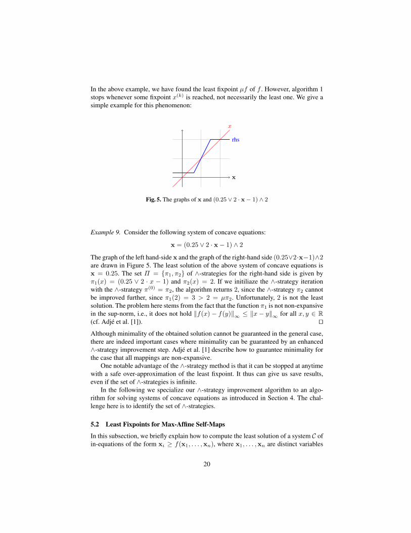
Fig. 5. The graphs of x and (0.25 ∨ 2 · x− 1) ∧ 2
Example 9. Consider the following system of concave equations:
x = (0.25 ∨ 2 · x− 1) ∧ 2
The graph of the left hand-side x and the graph of the right-hand side (0.25∨2·x−1)∧2are drawn in Figure 5. The least solution of the above system of concave equations isx = 0.25. The set Π = {π1, π2} of ∧-strategies for the right-hand side is given byπ1(x) = (0.25 ∨ 2 · x − 1) and π2(x) = 2. If we initiliaze the ∧-strategy iterationwith the ∧-strategy π(0) = π2, the algorithm returns 2, since the ∧-strategy π2 cannotbe improved further, since π1(2) = 3 > 2 = µπ2. Unfortunately, 2 is not the leastsolution. The problem here stems from the fact that the function π1 is not non-expansivein the sup-norm, i.e., it does not hold ‖f(x)− f(y)‖∞ ≤ ‖x− y‖∞ for all x, y ∈ R(cf. Adje et al. [1]). utAlthough minimality of the obtained solution cannot be guaranteed in the general case,there are indeed important cases where minimality can be guaranteed by an enhanced∧-strategy improvement step. Adje et al. [1] describe how to guarantee minimality forthe case that all mappings are non-expansive.
One notable advantage of the ∧-strategy method is that it can be stopped at anytimewith a safe over-approximation of the least fixpoint. It thus can give us save results,even if the set of ∧-strategies is infinite.
In the following we specialize our ∧-strategy improvement algorithm to an algo-rithm for solving systems of concave equations as introduced in Section 4. The chal-lenge here is to identify the set of ∧-strategies.
5.2 Least Fixpoints for Max-Affine Self-Maps
In this subsection, we briefly explain how to compute the least solution of a system C ofin-equations of the form xi ≥ f(x1, . . . ,xn), where x1, . . . ,xn are distinct variables
20

and f : Rn → R is monotone and affine. A function f : Rn → R is monotoneand affine iff there exist c0 ∈ R and c1, . . . , cn ∈ R≥0 such that f(x1, . . . , xn) =c0 + c1 · x1 + · · · + cn · xn for all x1, . . . , xn ∈ R. Here, we use the convention−∞+∞ = −∞.
For simplicity we assume that the least solution ρ∗ of C maps every variable to avalue that is strictly greater than −∞, i.e., ρ∗(x) > −∞ for all variable x. We cando so w.o.l.g., since we can determine the variables that are −∞ in the least solutionby performing n Kleene iteration steps. Then we can remove these variables and thecorresponding in-equations from the system of in-equations.
Let X denote the set of variables, and G = (X,→) be the variable dependencygraph of the system C of in-equations, i.e., the nodes of G are the variables of E andwe write xi → xj iff xi = ∞ implies xj = ∞, i.e., if there exists an in-equationxj ≥ f(x1, . . . ,xn) with f(x1, . . . , xn) = c0 +c1 ·x1 + · · ·+cn ·xn, where c0 > −∞and ci > 0. If G is strongly connected, then the least solution of E can be determinedby solving the following linear programming problem:
minn∑i=1
xi y ≥ f(x1, . . . ,xn) for all in-equations y ≥ f(x1, . . . ,xn) ∈ C
The above linear program aims at minimizing the sum of all variables x ∈ X. Thefeasible space is simply the set of all solutions of the system C of in-equations. If thislinear program is infeasible, then ρ∗(x) = ∞ holds for all variables x ∈ X. If thislinear program is feasible, then ρ∗ is the uniquely determined optimal solution:
Lemma 6. If the variable dependency graph of C is strongly connected, then the leastsolution of C can be computed by solving a linear programming problem that can beconstructed in linear time.
For computing the least solution in case that the variable dependency graph of C is notstrongly connected we divide the system of in-equations into strongly connected com-ponents. We start with an arbitrary non-trivial strongly connected component withoutincomming edges. Thus, according to Lemma 6, we can compute the least solution ofthe induced system of in-equations by solving a linear programming problem that canbe constructed in linear time. After we have determined the values for this strongly con-nected component, we can replace these variables with their values. We can repeat theabove procedure until all strongly connected components are solved. Since the num-ber of strongly connected components is bounded by the number of variables, we haveshown the following:
Theorem 1 (Gaubert et al. [9]). The least solution of a system of in-equations of theform xi ≥ f(x1, . . . ,xn), where f is a monotone and affine operator, can be com-puted by solving linearly many linear programming problems, each of which can beconstructed in linear time. Thus, it can be computed in polynomial time. ut
Example 10. We consider the following system of in-equations:
x1 ≥ −10 x1 ≥14· x2 + 1 x2 ≥ 2 · x1 x3 ≥ x3 + x1 − 1 x3 ≥ 0
21

Our goal is to compute the least solution using the method presented in this subsection.The strongly connected components of the variable dependency graph are {x1,x2} and{x3}. The variables x1 and x2 do not depend on the variable x3. Thus, in the first stepwe have to compute the uniquely determined optimal solution of the following linearprogramming problem:
min x1 + x2 x1 ≥ −10 x1 ≥14· x2 + 1 x2 ≥ 2 · x1
The uniquely determined optimal solution gives us x1 = 2 and x2 = 4. After substitut-ing the variables x1 and x2 with their values, it remains to compute the least solutionof the following system of in-equations:
x3 ≥ x3 + 2− 1 ∨ 0
Thus, we have to determine the uniquely determined optimal solution of the followinglinear programming problem:
min x3 x3 ≥ x3 + 1 x3 ≥ 0
This linear programming problem is infeasible. Thus, we get x3 =∞. Hence, the leastsolution of the original system of in-equations is x1 = 2, x2 = 4, and x3 =∞. ut
When we use interior point methods for solving the linear programming problems, weobtain a polynomial-time algorithm. However, the number of arithmetic operations andmemory accesses then depends on the sizes of the occurring numbers. Thus, the algo-rithm is not uniform. A uniform polynomial-time algorithm is not known.
5.3 ∧-Strategies for Systems of Concave Equations
We aim at specializing our ∧-strategy improvement algorithm to an algorithm for solv-ing systems of concave equations as introduced in Section 4. For that, let us considerthe following system of concave equations:
x1 = f1,1(x1, . . . ,xn) ∨ · · · ∨ f1,k1(x1, . . . ,xn)...
xn = fn,1(x1, . . . ,xn) ∨ · · · ∨ f1,kn(x1, . . . ,xn)
Firstly, we have to define an adequate set Π of ∧-strategies for the function
f =
f1,1 ∨ · · · ∨ f1,k1...
fn,1 ∨ · · · ∨ fn,kn
: Rn → Rn,
where we expect that we can compute the least fixpoint µπ for every ∧-strategy π ∈ Πefficiently. We proceed as follows: We define the set Tk,1 as the smallest set that containsthe following functions:
22

1. All monotone and affine functions f : Rk → R, i.e. functions of the form f(x) =a>x+ b with a ∈ Rk≥0 and b ∈ R.
2. For all y ∈ Rk, the function fy : Rk → R that is defined by
fy(x) =
{−∞ if x ≤ y∞ if x > y
for all x ∈ Rk.
The set T ∨k,1 is then defined by T ∨k,1 := {f1 ∨ · · · ∨ fl | f1, . . . , fl ∈ Tk,1}. The set T ∨k,mis finally defined by T ∨k,m := {(f1, . . . , fm)> | f1, . . . , fm ∈ T ∨k,1}.
Let f = (f1, . . . , fn)>, where f1, . . . , fn : Rn → R are monotone and concave.The set Π of ∧-strategies for f is defined as follows:
Π = {π : T ∨n,n | π ≥ f}.
Each ∧-strategy π ∈ Π is a finite maximum of affine functions. It is thus in particularconvex. As we have seen in Section 5.2, the least fixpoint µπ of a ∧-strategy π can becomputed through linear programming (cf. Gaubert et al. [9]). Because f ≤ π holds forall π ∈ Π , it follows µf ≤ µπ for all π ∈ Π . Moreover, because each component of fis a maximum of finitely many concave functions, it follows that there indeed exists a πwith µπ = µf . Hence, Π admits lower selections. We have µf = min {µπ | π ∈ Π}as desired.
Note that Π can be indeed infinite. However, in some cases there exists a finitesubset Π ′ of Π such that f(x) = min {π(x) | π ∈ Π ′} for all x ∈ Rn (cf. Gaubertet al. [9]). Then we can restrict our considerations to this finite subset.
5.4 Improving ∧-Strategies
In order to use Algorithm 1, it remains to explain how we can realize the ∧-strategyimprovement step (Step 4). We assume that we have given a post-fixpoint x of f , i.e.,x ≥ f(x). Our goal is to compute a ∧-strategy π ∈ Π such that π(x) = f(x), i.e., π islocally optimal at x. In other words: we have to find a lower selection.
For that, we assume that for any monotone and concave function f : Rk → R andany x ∈ (R ∪ {∞})k with −∞ < f(x) <∞, Tf,x : Rk → R denotes a monotone andaffine function such that
Tf,x ≥ f, and Tf,x(x) = f(x).
The function Tf,x must exist due to the monotonicity and concavity of f . For the sake
of simplicity of the presentation we omit the case that x /∈ (R∪{∞})k. For all x ∈ Rk
with f(x) = ∞, we additionally set Tf,x(y) = ∞ for all y ∈ Rk, and for all x ∈ Rk
with f(x) = −∞, we set
Tf,x(y) =
{−∞ if y ≤ x∞ if y > x
23

For f = f1 ∨ · · · ∨ fk with f1, ..., fk : Rk → R monotone and concave, we set
Tf,x := Tf1,x ∨ · · · ∨ Tfk,x for all x ∈ Rk.
Moreover, for f = (f1, . . . , fn)T with f1, . . . , fn : Rk → R we set
Tf,x = (Tf1,x, . . . , Tfn,x)>
Then, we have:
Lemma 7. Tf,x ≥ f and Tf,x(x) = f(x) for all x ∈ Rn. ut
Therefore, Tf,x is a ∧-strategy for f that is locally optimal at x. However, it remains toanswer the question how Tf,x can be computed.
Let f : Rn → R be concave, and x ∈ Rn with−∞ < f(x) <∞. For simplicity weassume that x ∈ Rn. We can do so w.l.o.g., since we can remove the other componentsand treat them separately. Our goal is to compute an affine function Tf,x : Rn → Rsuch that Tf,x(x) = f(x) and Tf,x ≥ f . Hence,
Tf,x(y) = f(x) + d>(y − x) for all y ∈ Rn
Hence, we are searching for a d ∈ Rn such that
g(d) := sup {g(d, y) | y ∈ Rn} ≤ f(x)
holds, where g(d, y) := f(y) − d>(y − x). The function g is convex, since it is thesupremum of a set of affine functions. For computing the value g(d) for a given d ∈Rn, we have to solve an unconstraint convex optimization problem, because g(d, ·) isconcave and thus−g(d, ·) is convex. However, this does not lead to an practical methodfor our application mentioned in Section 3.
For our application described in Section 3, we have to consider the case that f :Rn → R is given by
f(x) = sup {C •X | X � 0,A(X) = a,B(X) ≤ x},
i.e., f(x) is given by the optimal value of the following SDP problem:
maxX
C •X A(X) = a B(X) ≤ x X � 0
Note that f is monotone. We moreover assume that −∞ < f(x) < ∞ holds. Forsimplicity we again assume that x ∈ Rn. We can deal with the other cases by removingconstraints from the semi-definite programming problem. We aim at using the dualproblem in order to compute Tf,x. The dual problem (see e.g. Todd [22]) is given by:
minλ,µ
x>λ+ a>µ Bλ+Aµ � C λ ≥ 0
Here, the column vectors λ and µ are the variables. Let d(x) denote the optimal value ofthe dual problem. Weak duality gives us f(x) ≤ d(x). By assumption we in particularhave −∞ < d(x).
24

Now we define a hyperplane Tf,x as follows. If d(x) =∞, i.e., if the dual is infea-sible, then we set
Tf,x(z) =∞ for all z ∈ Rn
Finally, assume −∞ < d(x) < ∞. If the dual has an optimal solution (λ, µ), then wedefine the hyperplane Tf,x by
Tf,x(z) = λ>z + µ>a for all z ∈ Rn
If the dual has no optimal solution, we in practice simply choose a good feasible solu-tion. Weak duality gives us Tf,x ≥ f .
Observe that Tf,x is monotone, because λ ≥ 0. In order to conclude Tf,x(x) =f(x), we however need stronger assumptions. For instance assumptions that implystrong duality. One sufficient criterion for strong duality and the existence of an op-timal solution for the dual problem is that all components ofA are linearly independentand {X � 0 | A(X) = a, B(X)C x} 6= ∅ (cf. Todd [22]).
The result of the above discussion can be summarized as follows: we can computea self-map Tf,x that fulfills the statements of Lemma 7 (i.e., Tf,x ≥ f and Tf,x(x) =f(x)) through semi-definite programming, whenever the above sufficient condition forstrong duality is fulfilled.
5.5 The Harmonic Oscillator
We continue Example 4 (page 15), i.e., in order to analyze the harmonic oscillator weaim at solving the following systems of equations:
xst,p1 = 0 ∨ (JsKR{p 7→ xst,p | p ∈ P})(p1)
xst,p2 = 1 ∨ (JsKR{p 7→ xst,p | p ∈ P})(p2)
xst,p3 = 0 ∨ (JsKR{p 7→ xst,p | p ∈ P})(p3)
xst,p4 = 1 ∨ (JsKR{p 7→ xst,p | p ∈ P})(p4)
xst,p5 = 7 ∨ (JsKR{p 7→ xst,p | p ∈ P})(p5)
We emphasize that the right-hand sides are finite maximums of monotone and concavefunctions. It is easy to verify that xst,p1 = · · · = xst,p4 = ∞, xst,p5 = 7 is a post-solution. In oder to simplify notations, let c1 = c3 = 0, c2 = c4 = 1, c5 = 7, and, forall i ∈ {1, . . . , 5}, fi : Rn → R be defined by
fi((x1, . . . , x5)>) := ci ∨ (JsKR{pi 7→ xi | i ∈ {1, . . . , 5}})(pi)
Let moreover f = (f1, . . . , f5)>, i.e., f denotes the right-hand side of the above systemof equations. If we evaluate the right-hand sides, we get
f((∞,∞,∞,∞, 7)>) ' (2.0426, 2.0426, 1.6651, 1.6651, 7)>.
25

For evaluating the right-hand sides, we can use semi-definite programming. The usualimplementations solve the primal and the dual problem at the same time. From a dualoptimal solution, we obtain our first ∧-strategy π(0) that is given as follows:
π(0) := Tf,(∞,∞,∞,∞,7)>((x1, . . . , x5)>) '
0 ∨ 0.14588 · x5 + 1.02141 ∨ 0.14588 · x5 + 1.02140 ∨ 0.11892 · x5 + 0.832631 ∨ 0.11892 · x5 + 0.83263
7 ∨ 0.99456 · x5
We are now going to explain how we have obtained the first component. According tothe findings from Example 4, we have
(JsKR{p1 7→ ∞, p2 7→ ∞, p3 7→ ∞, p4 7→ ∞, p5 7→ 7})(p1)= sup {C1 •X | X � 0, X1·1 = 1, B5 •X ≤ 7}
= sup
0 −0.5 −0.005−0.5 0 0−0.005 0 0
•X | X � 0, X1·1 = 1,
0 0 00 2 10 1 3
•X ≤ 7
=2.0426
We have seen in Subsection 5.4, that, in order to compute an affine over-approximationof (JsKR{pi 7→ xi | i ∈ {1, . . . , 5}})(pi) that is exact at x1 = x2 = x3 = x4 =∞ andx5 = 7, we can solve the dual problem that is given as follows:
inf
7λ+ µ | λ ≥ 0, µ ∈ R, λB5 + µ
1 0 00 0 00 0 0
� C1
= inf {7λ+ µ | λ ≥ 0, µ ∈ R,
λ
0 0 00 2 10 1 3
+ µ
1 0 00 0 00 0 0
� 0 −0.5 −0.005−0.5 0 0−0.005 0 0
Running a solver may give us the result λ ' 0.14588 and µ ' 1.0214. This gives usthe first component of π(0). The remaining components can be computed in the sameway.
As described in Subsection 5.2 we can compute the least fixpoint of π(0) throughlinear programming. We get
x(0) := µπ(0) = (2.0426, 2.0426, 1.6651, 1.6651, 7)>.
Then, by again solving semi-definite and linear programming problems, we get
π(1) := Tf,x(0)((x1, . . . , x5)>) '
0 ∨ 0.90541 · x1 + 0.01340 · x5 + 0.0938201 ∨ 0.90541 · x2 + 0.01340 · x5 + 0.0938190 ∨ 0.88297 · x3 + 0.01346 · x5 + 0.0942051 ∨ 0.88297 · x4 + 0.01346 · x5 + 0.094205
7 ∨ 0.99456 · x5
26

and
x(1) := µπ(1) ' (1.9838, 1.9838, 1.6098, 1.6098, 7.0000)>.
Continuing this process, we find:
x(2) := µπ(2) ' (1.8971, 1.8971, 1.5434, 1.5434, 7.0000)>
x(3) := µπ(3) ' (1.8718, 1.8718, 1.5280, 1.5280, 7.0000)>
x(4) := µπ(4) ' (1.8708, 1.8708, 1.5275, 1.5275, 7.0000)>
x(5) := µπ(5) ' (1.8708, 1.8708, 1.5275, 1.5275, 7.0000)>
{−2.0462 ≤ x ≤ 2.0426, −1.665 ≤ v ≤ 1.665, 2x2 + 3v2 + 2xv ≤ 7}{−1.9838 ≤ x ≤ 1.9838, −1.6097 ≤ v ≤ 1.6097, 2x2 + 3v2 + 2xv ≤ 7}
{−1.8971 ≤ x ≤ 1.8971, −1.5435 ≤ v ≤ 1.5435, 2x2 + 3v2 + 2xv ≤ 7}{−1.8718 ≤ x ≤ 1.8718, −1.5275 ≤ v ≤ 1.5275, 2x2 + 3v2 + 2xv ≤ 7}
{−1.8708 ≤ x ≤ 1.8708, −1.5275 ≤ v ≤ 1.5275, 2x2 + 3v2 + 2xv ≤ 7}
Fig. 6. Visualization of a run of our ∧-strategy iteration algorithm for the harmonic oscillatorfrom Section 2
Our ∧-strategy iteration stabilizes after a few iterations. The run of our ∧-strategy im-provement algorithm is visualized in Figure 6. As a result, we obtain
µf ≤ (1.8708, 1.8708, 1.5275, 1.5275, 7.0000)>.
As a result we finally obtain that the following invariants hold at program point st ofthe harmonic oscillator (page 4):
−x1 ≤ 1.8708 x1 ≤ 1.8708 −x2 ≤ 1.5275
x2 ≤ 1.5275 2x21 + 3x2
2 + 2x1x2 ≤ 7
27
6 The Max-Strategy Iteration Approach
Before giving a formal description of the max-strategy iteration approach in Subsec-tion 6.2, we explain it by a simple example in Subsection 6.1. In Subsection 6.3 wefinally apply the max-strategy iteration approach to the harmonic oscillator introducedin Section 2.
6.1 A Simple Example
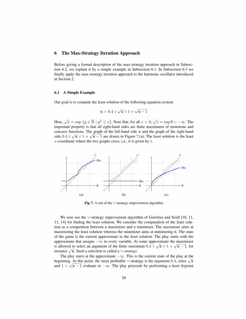
Our goal is to compute the least solution of the following equation system:
x = 0.4 ∨√
x ∨ 1 +√
x− 1
Here,√x = sup {y ∈ R | y2 ≤ x}. Note that, for all x < 0,
√x = sup ∅ = −∞. The
important property is that all right-hand sides are finite maximums of monotone andconcave functions. The graph of the left-hand side x and the graph of the right-handside 0.4 ∨ √x ∨ 1 +
√x− 1 are drawn in Figure 7.(a). The least solution is the least
x-coordinate where the two graphs cross, i.e., it is given by 1.
x
x
rhs
x
x
rhs
rhsx
x
rhs
rhs
(a) (b) (c)
Fig. 7. A run of the ∨-strategy improvement algorithm
We now use the ∨-strategy improvement algorithm of Gawlitza and Seidl [10, 11,13, 14] for finding the least solution. We consider the computation of the least solu-tion as a competition between a maximizer and a minimizer. The maximizer aims atmaximizing the least solution whereas the minimizer aims at minimizing it. The stateof the game is the current approximate to the least solution. The play starts with theapproximate that assigns −∞ to every variable. At some approximate the maximizeris allowed to select an argument of the finite maximum 0.4 ∨ √x ∨ 1 +
√x− 1, for
instance√
x. Such a selection is called a ∨-strategy.The play starts at the approximate −∞. This is the current state of the play at the
beginning. At this point, the most profitable ∨-strategy is the argument 0.4, since√
xand 1 +
√x− 1 evaluate to −∞. The play proceeds by performing a least fixpoint
28

iteration starting at −∞ using the current ∨-strategy, i.e., the next approximate is theleast solution of the equation system
x = 0.4
that exceeds −∞. Hence, the next approximate is 0.4 (cf. Figure 7.(b)). Note that 0.4is not only the least solution of the equation system x = 0.4 that exceeds 0.4, but it isalso the greatest solution of the inequation x ≤ 0.4, i.e., the greatest point in the convexarea that is above the graph of the left hand-side and below the graph of the concaveright-handside (cf. Figure 7.(b)). This is not by accident. We will see that during a runof our ∨-strategy improvement algorithm, the next approximate is always the greatestpoint of such a convex area. This implies that it can be computed through algorithmsfor solving convex optimization problems.
Now, we try to improve the current ∨-strategy locally at 0.4. Since√
0.4 > 0.4holds, we can improve the current ∨-strategy to the ∨-strategy that selects the argument√
x.8 This gives us a strict local improvement. Thus, the next approximate is the leastsolution of the equation system
x =√
x
that exceeds 0.4. Hence, the next approximate is 1 (cf. Figure 7.(c)). It is again thegreatest solution of the inequation system x ≤ √x. Thus, it is the uniquely determinedoptimal solution of the following convex optimization problem:
max x x2 − x ≤ 0
In this case the unique optimal solution can for instance be computed through semi-definite programming, because it is a convex quadratic optimization problem.
Now, our current approximate is 1 and our current ∨-strategy selects the argument√x. We now again try to improve our current ∨-strategy, i.e., we search for a ∨-strategy
that is strictly more profitable at our current approximate 1 than our current ∨-strategy.Since 0.4 < 1 = 1 +
√1− 1 = 1 =
√1 holds, there is no such ∨-strategy. In other
words: The current∨-strategy cannot be improved at the current approximate (cf. Figure7.(c)). This means: We have found a solution of the equation system
x = 0.4 ∨√
x ∨ 1 +√
x− 1.
Since the sequence of approximates is monotonically increasing and bounded by theleast solution, we in fact have found the least solution. For short: The ∨-strategy im-provement algorithm terminates and returns the least solution 1.
6.2 The Max-Strategy Improvement Algorithm
In this section we are going to compute least solutions of systems of concave equationsthrough the ∨-strategy improvement algorithm of Gawlitza and Seidl [10, 11, 12, 14].
8 Since 1 +√
0.4− 1 = 1 +√−0.6 = 1 +−∞ = −∞ holds, a switch to the ∨-strategy that
selects the argument 1 +√
x− 1 is not profitable at the approximate 0.4.
29

Systems of concave equations are in particular systems of monotone equations over thecomplete linearly ordered set R. For the sake of generality, we subsequently consideran arbitrary complete linearly ordered set.
A ∨-strategy σ for a system E of monotone equations over a complete linearlyordered set is a function that maps every expression e1 ∨ · · · ∨ ek occurring in E toone of the immediate sub-expressions ej , j ∈ {1, . . . , k}. We denote the set of all ∨-strategies for E by ΣE . We drop the subscript, whenever it is clear from the context.Finally, we set
E(σ) := {x = σ(e) | x = e ∈ E}.
Example 11. For the system E = {x = 12 ∨√
x} of concave equations and the ∨-strategy σ = { 1
2 ∨√
x 7→ 12}, we have E(σ) = {x = 1
2}. ut
Our ∨-strategy improvement algorithm iterates over ∨-strategies. It maintains a current∨-strategy and a current approximate to the least solution. In each step, if possible,the current ∨-strategy is improved w.r.t. the current approximate, and a new currentapproximate is computed w.r.t. the new current ∨-strategy and the current approximate:
Definition 2 (Improvements). Let E be a system of monotone equations over a com-plete linearly ordered set. Let σ, σ′ ∈ Σ be ∨-strategies for E and ρ be a pre-solution ofE(σ). The ∨-strategy σ′ is called improvement of σ w.r.t. ρ iff the following conditionsare fulfilled:
1. If ρ /∈ Sol(E), then JE(σ′)Kρ > ρ.
2. For all ∨-expressions e1 ∨ · · · ∨ ek occurring in E the following holds:
If σ′(e) 6= σ(e), then Jσ′(e)Kρ > Jσ(e)Kρ. ut
In many cases there exist several, different improvements of a ∨-strategy σ w.r.t. a pre-solution ρ of E(σ). Under the assumption that the operator ∨ is only used in its binaryversion, one is known as all profitable switches (see e.g. Bjorklund et al. [3, 4]). Carriedover to the case considered here, this means, that the ∨-strategy σ will be modified atany ∨-expression e1 ∨ e2 with Je1 ∨ e2Kρ > Jσ(e1 ∨ e2)Kρ. According to definition 2the selection at the other ∨-expressions must be preserved.
We can now formulate the ∨-strategy improvement algorithm for computing leastsolutions of systems of monotone equations over complete linearly ordered sets. Theinput is a system E of monotone equations over a complete linearly ordered set, a ∨-
30

strategy σinit for E , and a pre-solution ρinit of E(σinit). In order to compute the leastand not just some solution, we additionally require that ρinit ≤ µJEK holds:
Algorithm 2 The ∨-Strategy Improvement Algorithm
Input :
8<:- A system E of monotone equations over a complete linearly ordered set- A ∨-strategy σinit for E- A pre-solution ρinit of E(σinit) with ρinit ≤ µJEK
Output : The least solution µJEK of Eσ ← σinit;ρ← ρinit;
while (ρ /∈ Sol(E)) {σ ← improvement of σ w.r.t. ρ;ρ← µ≥ρJE(σ)K;
}return ρ;
Lemma 8. Let E be a system of monotone equations over a complete linearly orderedset. For i ∈ N, let ρi be the value of the program variable ρ and σi be the value of theprogram variable σ in the ∨-strategy improvement algorithm (Algorithm 2) after thei-th evaluation of the loop-body. The following statements hold for all i ∈ N:
1. ρi ≤ µJEK.2. ρi ∈ PreSol(E(σi+1)).3. ρi+1 = µ≥ρi
JE(σi+1)K.4. If ρi < µJEK, then ρi+1 > ρi.5. If ρi = µJEK, then ρi+1 = ρi. ut
An immediate consequence of Lemma 8 is the following lemma:
Lemma 9. Whenever the ∨-strategy improvement algorithm terminates, it computesthe least solution µJEK of E . utIn the following we are interested in solving systems of concave equations throughour ∨-strategy improvement algorithm. Hence, assume that E is a system of concaveequations. In this case our ∨-strategy improvement algorithm terminates and returnsthe least solution at the latest after considering every ∨-strategy at most |X| times.
In order to start our ∨-strategy improvement algorithm in a feasible area (see Gawl-itza and Seidl [13] for detailed explanations), we start the ∨-strategy improvement al-gorithm with the system
E ∨ −∞ := {x = e ∨ −∞ | x = e ∈ E},
the ∨-strategy
σinit = {e ∨ −∞ 7→ −∞ | x = e ∈ E},
and the pre-solution −∞ of (E ∨ −∞)(σinit). For i ∈ N, let ρi be the value of theprogram variable ρ and σi be the value of the program variable σ in the ∨-strategyimprovement algorithm (Algorithm 2) after the i-th evaluation of the loop-body. For alli ∈ N, the value ρi+1 = µ≥ρi
JE(σi+1)K is determined as follows:
31

Lemma 10. Let
X−∞ := {x ∈ X | x = e ∈ E(σi+1) and JeKρi = −∞}X∞ := {x ∈ X | x = e ∈ E(σi+1) and JeKρi =∞}X′ := X \ (X−∞ ∪X∞)
E ′ := {x = e ∈ E(σi+1) | x ∈ X′}[−∞/X−∞][∞/X∞].
Here, {x = e ∈ E(σi+1) | x ∈ X′}[−∞/X−∞][∞/X∞] denotes the system of basicconcave equations that is obtained from E(σi+1) by removing all equations x = e withx /∈ X′ and then replacing all occurrences of variables from X−∞ in the right-handsides with the constant−∞ and all occurrences of variables from X∞ in the right-handsides with the constant∞. Then
ρi+1(x′) = µ≥ρiJE(σi+1)K(x′)
= µ≥ρi|X′ JE′K(x′)
= sup {ρ(x′) | ρ : X′ → R and ρ(x) ≤ JeKρ for all equations x = e ∈ E ′}
for all x′ ∈ X′. Moreover, ρi+1(x−∞) = µ≥ρiJE(σi+1)K(x−∞) = −∞ for all x−∞ ∈
X−∞, and ρi+1(x∞) = µ≥ρiJE(σi+1)K(x∞) =∞ for all x∞ ∈ X∞,
Hence, provided that E is a system of concave equations, ρi+1 can be computed bysolving |X| convex optimization problems. Moreover, it is important to note that ρi+1
is uniquely determined through the system E , the ∨-strategy σi+1 and the set X∞ of allvariables that are already known to be∞. utSince the sequence ((ρi, {x ∈ X | x = e ∈ E(σi+1) and JeKρi =∞}))i is strictly in-creasing (ordered component-wise), Lemma 10 implies that the ∨-strategy improve-ment algorithm considers each ∨-strategy at most |X| times. Thus, we have shown thefollowing theorem:
Theorem 2. Let E be a system of concave equations. Our ∨-strategy improvement al-gorithm (Algorithm 2) computes the least solution µJEK of E and performs at most(|Σ|+ |X|) · |X| ∨-strategy improvement steps. If E is a system of concave equations,we have to solve |X| convex optimization problems for every ∨-strategy improvementstep. utExample 12. We consider the system
E ={x = −∞∨ 1
2 ∨√
x ∨ 78 +
√x− 47
64
}of concave equations. We start with the uniquely determined ∨-strategy σ0 such that
E(σ0) = {x = −∞}
and with the solution ρ0 := {x 7→ −∞} of E(σ0). Since ρ0 /∈ Sol(E), we improve the∨-strategy σ0 w.r.t. ρ0 to a ∨-strategy σ1 . Necessarily, we get
E(σ1) ={x =
12
}.
32
By Lemma 10, we get
ρ1(x) = µ≥ρ0JE(σ1)K(x) = sup{x | x ≤ 1
2
}.
Thus, ρ1 = {x 7→ 12}. Since
√12 > 1
2 and 78 +
√12 − 47
64 < 12 hold, we necessarily
improve the ∨-strategy σ1 w.r.t. ρ1 to the uniquely determined ∨-strategy σ2 such that
E(σ2) ={x =√
x}.
Again by Lemma 10, we get
ρ2(x) = µ≥ρ1JE(σ2)K(x) = sup{x | x ≤
√x}
= 1.
Thus, ρ2 = {x 7→ 1}. Since
78
+
√1− 47
64>
78
+
√1− 60
64=
98> 1,
we get
E(σ3) =
{x =
78
+
√x− 47
64
}.
Again by Lemma 10, we get
ρ3(x) = µ≥ρ2JE(σ3)K(x) = sup
{x | x ≤ 7
8+
√x− 47
64
}= 2.
Thus, we finally get ρ3 = {x 7→ 2}. The algorithm terminates, because ρ3 solves E .Thus, ρ3 = µJEK. We have found the least solution.
In each step we had to solve convex optimization problems that can be solvedthrough semi-definite programming (c.f. Gawlitza and Seidl [13]). ut
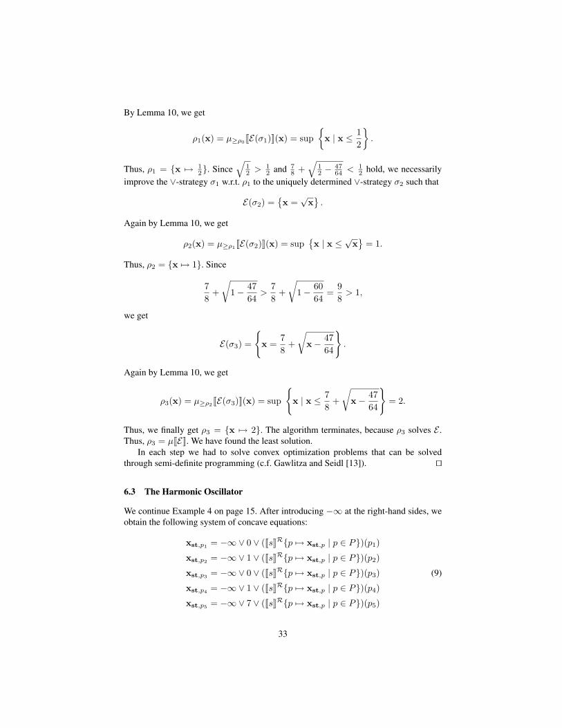
6.3 The Harmonic Oscillator
We continue Example 4 on page 15. After introducing −∞ at the right-hand sides, weobtain the following system of concave equations:
xst,p1 = −∞∨ 0 ∨ (JsKR{p 7→ xst,p | p ∈ P})(p1)
xst,p2 = −∞∨ 1 ∨ (JsKR{p 7→ xst,p | p ∈ P})(p2)
xst,p3 = −∞∨ 0 ∨ (JsKR{p 7→ xst,p | p ∈ P})(p3) (9)
xst,p4 = −∞∨ 1 ∨ (JsKR{p 7→ xst,p | p ∈ P})(p4)
xst,p5 = −∞∨ 7 ∨ (JsKR{p 7→ xst,p | p ∈ P})(p5)
33

In this example we have 35 = 243 different ∨-strategies. It is clear that the algorithmwill switch to the ∨-strategy that is given by the finite constants in the first step. At eachequation, it then can switch to the non-constant expression, but then, because it con-structs a strictly increasing sequence, it can never return to the constant. Summarizing,because of the simple structure, it is clear that our ∨-strategy improvement algorithmwill perform at most 6 ∨-strategy improvement steps. In fact our prototypical imple-mentation performs 4 ∨-strategy improvement steps when solving this example. Thelast ∨-strategy that the algorithm considers leads to the system
xst,p1 = (JsKR{p 7→ xst,p | p ∈ P})(p1)
xst,p2 = (JsKR{p 7→ xst,p | p ∈ P})(p2)
xst,p3 = (JsKR{p 7→ xst,p | p ∈ P})(p3)
xst,p4 = (JsKR{p 7→ xst,p | p ∈ P})(p4)xst,p5 = 7
of basic concave equations. The current approximate at this point of time does notassign∞ to any variable. Because of Lemma 10, in order to determine the next valuefor the variable xst,pk
(for k ∈ {1, . . . , 5}), we solve the following convex optimizationproblem
sup {ρ(xst,pk) | ρ : X→ R and
ρ(xst,pi) ≤ (JsKR{q 7→ ρ(xst,q) | q ∈ P})(pi), i ∈ {1, . . . , 4} andxst,p5 ≤ 7}
For that, we solve the following semi-definite programming problem, that is obtainedfrom the above convex optimization problem through unfolding the definition of therelaxed abstract semantics:
sup xst,pk
xst,p1 ≤ Ck •X(1) X(1) � 0 X(1)1·1 = 1
B1 •X(1) ≤ xst,p1 · · · B5 •X(1) ≤ xst,p5
xst,p2 ≤ Ck •X(2) X(2) � 0 X(2)1·1 = 1
B1 •X(2) ≤ xst,p1 · · · B5 •X(2) ≤ xst,p5
xst,p3 ≤ Ck •X(3) X(3) � 0 X(3)1·1 = 1
B1 •X(3) ≤ xst,p1 · · · B5 •X(3) ≤ xst,p5
xst,p4 ≤ Ck •X(4) X(4) � 0 X(4)1·1 = 1
B1 •X(4) ≤ xst,p1 · · · B5 •X(4) ≤ xst,p5
xst,p5 ≤ 7
The matrices B1, . . . , B5, C1, . . . , C5 are defined in Example 4 (page 15). Solving theabove semi-definite programming problem gives us the final values for the variables
34

xst,p1 , . . . ,xst,p5 . We get
µJEK = {xst,p1 7→ 1.8708..,xst,p2 7→ 1.8708..,xst,p3 7→ 1.5275..,xst,p4 7→ 1.5275..,xst,p5 7→ 7}
Hence, the following invariants hold at program point st of the harmonic oscillator (seepage 4):
−x1 ≤ 1.8708 x1 ≤ 1.8708 −x2 ≤ 1.5275
x2 ≤ 1.5275 2x21 + 3x2
2 + 2x1x2 ≤ 7
For this example the ∨-strategy improvement algorithm presented in this section findsthe same invariants as the ∧-strategy improvement algorithm presented in section 5 (cf.Subsection 5.5).
7 Comparison and Conclusion
In this paper we discussed how we can use strategy iteration for solving systems ofconcave equations. This class is a natural and strict generalization of systems of rationalequations (studied by Gawlitza and Seidl [10, 14]). In the context of static programanalysis, such equation systems are useful for approximating the abstract semantics ofprograms w.r.t. quadratic templates through semi-definite relaxations. We discussed twodifferent approaches that can be specialized for solving systems of concave equations:
For the studied case, the ∧-strategy approach of Adje et al. [2] successively approx-imates the given equation system by systems of affine in-equations which can be effi-ciently solved by linear programming. The resulting method works similar to Newton’smethod. For each approximate, an improved∧-strategy (a system of affine in-equations)can be efficiently determined through semi-definite programming.
As an alternative approach, we discussed the ∨-strategy improvement approach ofGawlitza and Seidl [10, 11]. From an algorithmic perspective these two approaches havequite distinct characteristics. ∨-strategy iteration, when applied to quadratic zones, ineach iteration combines one constraint for each program point and program variableinto a global semi-definite programming problem which is jointly solved by SDP.
The advantage of the ∨-strategy iteration approach is that (given an ideal SDPsolver) the number of iterations is guaranteed to be finite and that it guarantees min-imality of the obtained solution. The draw-back, however, is that only after termination,a safe invariant is found. Intermediate approximates to the least solution are not safe.
The ∧-strategy iteration approach on the other hand, when applied to quadratic tem-plates, relies on solving (dual) SDP problems locally for every constraint separately —each of which typically involves just few unknowns of the analysis problem. The globaltask of determining the next approximate for all program points and program variablesthen is delegated to LP solving. The disadvantage of the ∧-strategy iteration approach isthat the iteration is not guaranteed to terminate but only to converge to a solution. More-over, this solution is not necessarily minimal. On the other hand (again assuming idealsolvers for SDP and LP), it produces a decreasing sequence of post-fixpoints. Thus,
35

the iteration may any time be terminated with a valid program invariant. Moreover, thespeed of convergence is — as for Newton’s method — usually quite good. Another ad-vantage of the ∧-strategy iteration approach is that LP solvers in general scale to largerproblems than SDP solvers. Therefore, we expect the ∧-strategy iteration approach tobe applicable not just to small, but also to medium sized input programs. A detailedpractical comparison w.r.t. efficiency and precision, however, remains for future work.
Bibliography
[1] A. Adje, S. Gaubert, and E. Goubault. Computing the smallest fixed point ofnonexpansive mappings arising in game theory and static analysis of programs. InProceedings of the Eighteenth International Symposium on Mathematical Theoryof Networks and Systems (MTNS2008), 2008.
[2] A. Adje, S. Gaubert, and E. Goubault. Coupling policy iteration with semi-definiterelaxation to compute accurate numerical invariants in static analysis. In A. D.Gordon, editor, ESOP, volume 6012 of LNCS, pages 23–42. Springer, 2010. ISBN978-3-642-11956-9.
[3] H. Bjorklund, S. Sandberg, and S. Vorobyov. Optimization on completely uni-modal hypercubes. Technichal report 2002-18, Department of Information Tech-nology, Uppsala University, 2002.
[4] H. Bjorklund, S. Sandberg, and S. Vorobyov. Complexity of Model Checkingby Iterative Improvement: the Pseudo-Boolean Framework . In Proc. 5th Int.Andrei Ershov Memorial Conf. Perspectives of System Informatics, pages 381–394. LNCS 2890, Springer, 2003.
[5] S. Boyd and L. Vandenberghe. Convex Optimization. Cambridge University Press,2004.
[6] A. Costan, S. Gaubert, E. Goubault, M. Martel, and S. Putot. A Policy Itera-tion Algorithm for Computing Fixed Points in Static Analysis of Programs. InComputer Aided Verification, 17th Int. Conf. (CAV), pages 462–475. LNCS 3576,Springer Verlag, 2005.
[7] E. Feron and F. Alegre. Control software analysis, part i open-loop properties.CoRR, abs/0809.4812, 2008.
[8] E. Feron and F. Alegre. Control software analysis, part ii: Closed-loop analysis.CoRR, abs/0812.1986, 2008.
[9] S. Gaubert, E. Goubault, A. Taly, and S. Zennou. Static analysis by policy iterationon relational domains. In Nicola [17], pages 237–252. ISBN 978-3-540-71314-2.
[10] T. Gawlitza and H. Seidl. Precise relational invariants through strategy iteration.In J. Duparc and T. A. Henzinger, editors, CSL, volume 4646 of LNCS, pages23–40. Springer, 2007. ISBN 978-3-540-74914-1.
[11] T. Gawlitza and H. Seidl. Precise fixpoint computation through strategy iteration.In Nicola [17], pages 300–315. ISBN 978-3-540-71314-2.
[12] T. Gawlitza and H. Seidl. Precise interval analysis vs. parity games. In J. Cuellar,T. S. E. Maibaum, and K. Sere, editors, FM, volume 5014 of LNCS, pages 342–357. Springer, 2008. ISBN 978-3-540-68235-6.
36

[13] T. M. Gawlitza and H. Seidl. Computing relaxed abstract semantics w.r.t. quadraticzones precisely. In R. Cousot and M. Martel, editors, SAS, volume 6337 of LectureNotes in Computer Science, pages 271–286. Springer, 2010. ISBN 978-3-642-15768-4.
[14] T. M. Gawlitza and H. Seidl. Solving systems of rational equations through strat-egy iteration. TOPLAS, (accepted, to appear).
[15] A. Mine. The octagon abstract domain. In WCRE, pages 310–, 2001.[16] A. Nemirovski. Modern Convex Optimization. Department ISYE, Georgia Insti-
tute of Technology, 2005.[17] R. D. Nicola, editor. Programming Languages and Systems, 16th European Sym-
posium on Programming, ESOP 2007, Held as Part of the Joint European Confer-ences on Theory and Practics of Software, ETAPS 2007, Braga, Portugal, March24 - April 1, 2007, Proceedings, volume 4421 of LNCS, 2007. Springer. ISBN978-3-540-71314-2.
[18] J. Ortega and W. Rheinboldt. Iterative solution of nonlinear equations in severalvariables. Academic Press, 1970.
[19] S. Sankaranarayanan, H. B. Sipma, and Z. Manna. Scalable analysis of linearsystems using mathematical programming. In R. Cousot, editor, VMCAI, volume3385 of LNCS, pages 25–41. Springer, 2005. ISBN 3-540-24297-X.
[20] S. Sankaranarayanan, M. Colon, H. B. Sipma, and Z. Manna. Efficient stronglyrelational polyhedral analysis. In E. A. Emerson and K. S. Namjoshi, editors,VMCAI, volume 3855 of Lecture Notes in Computer Science, pages 111–125.Springer, 2006. ISBN 3-540-31139-4.
[21] A. Schrijver. Theory of Linear and Integer Programming. Wiley, 1986.[22] M. J. Todd. Semidefinite optimization. Acta Numerica, 10:515–560, 2001.[23] S. A. Vavasis. Quadratic programming is in np. Inf. Process. Lett., 36(2):73–77,
1990.
37