quteprints.qut.edu.au/16436/1/christopher_mccool_thesis.pdf · abstract face verication is a...
TRANSCRIPT

Image and Video Laboratory
School of Engineering Systems
HYBRID 2D AND 3D FACE VERIFICATION
Christopher Steven McCoolB.Eng(Hons), B.InfoTech(Dist)
SUBMITTED AS A REQUIREMENT OF
THE DEGREE OF
DOCTOR OF PHILOSOPHY
AT
QUEENSLAND UNIVERSITY OF TECHNOLOGY
BRISBANE, QUEENSLAND
MAY 2007


Dedicated to the
memory of
Eleanor Omrah McCool
(1917 - 2007)
i

ii

Keywords
Computer Vision, Face Recognition, Two-Dimensional, Three-Dimensional, Multi-
Modal, Multi-Algorithm, Fusion, Pattern Recognition, Biometrics, Principal Compo-
nent Analysis, Two-Dimensional Discrete Cosine Transform, Classifier Fusion, Face
Verification, Feature Distribution Modelling and Gaussian Mixture Modelling.
iii

iv

Abstract
Face verification is a challenging pattern recognition problem. The face is a biomet-
ric that, we as humans, know can be recognised. However, the face is highly de-
formable and its appearance alters significantly when the pose, illumination or ex-
pression changes. These changes in appearance are most notable for texture images,
or two-dimensional (2D) data. But the underlying structure of the face, or three-
dimensional (3D) data, is not changed by pose or illumination variations.
Over the past five years methods have been been investigated to combine 2D and
3D face data to improve the accuracy and robustness of face verification. Much of
this research has examined the fusion of a 2D verification system and a 3D verification
system, known as multi-modal classifier score fusion. These verification systems usu-
ally compare two feature vectors (two image representations), a and b, using distance-
or angular-based similarity measures. However, this does not provide the most com-
plete description of the features being compared as the distances describe at best the
covariance of the data, or the second order statistics (for instance Mahalanobis based
measures).
A more complete description would be obtained by describing the distribution of
the feature vectors. However, feature distribution modelling is rarely applied to face
verification because a large number of observations is required to train the models.
This amount of data is usually unavailable and so this research examines two methods
for overcoming this data limitation:
1. the use of holistic difference vectors of the face, and
2. by dividing the 3D face into Free-Parts.
v

The permutations of the holistic difference vectors is formed so that more obser-
vations are obtained from a set of holistic features. On the other hand, by dividing the
face into parts and considering each part separately many observations are obtained
from each face image; this approach is referred to as the Free-Parts approach. The
extra observations from both these techniques are used to perform holistic feature dis-
tribution modelling and Free-Parts feature distribution modelling respectively. It is
shown that the feature distribution modelling of these features leads to an improved
3D face verification system and an effective 2D face verification system. Using these
two feature distribution techniques classifier score fusion is then examined.
This thesis also examines methods for performing classifier fusion score fusion.
Classifier score fusion attempts to combine complementary information from multiple
classifiers. This complementary information can be obtained in two ways: by us-
ing different algorithms (multi-algorithm fusion) to represent the same face data for
instance the 2D face data or by capturing the face data with different sensors (multi-
modal fusion) for instance capturing 2D and 3D face data. Multi-algorithm fusion is
approached as combining verification systems that use holistic features and local fea-
tures (Free-Parts) and multi-modal fusion examines the combination of 2D and 3D face
data using all of the investigated techniques.
The results of the fusion experiments show that multi-modal fusion leads to a con-
sistent improvement in performance. This is attributed to the fact that the data being
fused is collected by two different sensors, a camera and a laser scanner. In deriving
the multi-algorithm and multi-modal algorithms a consistent framework for fusion was
developed.
The consistent fusion framework, developed from the multi-algorithm and multi-
modal experiments, is used to combine multiple algorithms across multiple modalities.
This fusion method, referred to as hybrid fusion, is shown to provide improved per-
formance over either fusion system on its own. The experiments show that the final
hybrid face verification system reduces the False Rejection Rate from 8.59% for the
best 2D verification system and 4.48% for the best 3D verification system to 0.59% for
the hybrid verification system; at a False Acceptance Rate of 0.1%.
vi

Contents
Keywords iii
Abstract v
List of Tables xi
List of Figures xiv
List of Abbreviations xxi
List of Publications xxiii
Statement of Authorship xxv
Acknowledgements xxvii
1 Introduction 1
1.1 Motivation and Overview . . . . . . . . . . . . . . . . . . . . . . . . 1
1.2 Aims and Objectives . . . . . . . . . . . . . . . . . . . . . . . . . . 3
1.2.1 Feature Distribution Modelling . . . . . . . . . . . . . . . . . 3
1.2.2 Classifier Score Fusion . . . . . . . . . . . . . . . . . . . . . 4
1.3 Scope of Thesis . . . . . . . . . . . . . . . . . . . . . . . . . . . . . 5
1.3.1 Feature Distribution Modelling . . . . . . . . . . . . . . . . . 5
1.3.2 Classifier Score Fusion . . . . . . . . . . . . . . . . . . . . . 6
1.4 Original Contributions and Publications . . . . . . . . . . . . . . . . 6
1.5 Outline of Thesis . . . . . . . . . . . . . . . . . . . . . . . . . . . . 8
vii

2 Review of Face Verification 11
2.1 Introduction . . . . . . . . . . . . . . . . . . . . . . . . . . . . . . . 11
2.1.1 Overview of Face Verification . . . . . . . . . . . . . . . . . 14
2.2 Face Verification - 2D . . . . . . . . . . . . . . . . . . . . . . . . . . 17
2.2.1 Holistic Feature Extraction . . . . . . . . . . . . . . . . . . . 18
2.2.2 Local Feature Extraction . . . . . . . . . . . . . . . . . . . . 24
2.3 Face Verification - 3D . . . . . . . . . . . . . . . . . . . . . . . . . . 28
2.3.1 Data Acquisition . . . . . . . . . . . . . . . . . . . . . . . . 29
2.3.2 Verification Methods . . . . . . . . . . . . . . . . . . . . . . 33
2.4 Multi-Modal Person Verification . . . . . . . . . . . . . . . . . . . . 36
2.4.1 Multi-Modal Face Verification . . . . . . . . . . . . . . . . . 41
3 Experimental Framework 43
3.1 Introduction . . . . . . . . . . . . . . . . . . . . . . . . . . . . . . . 43
3.2 Database Description . . . . . . . . . . . . . . . . . . . . . . . . . . 44
3.3 Data Normalisation . . . . . . . . . . . . . . . . . . . . . . . . . . . 47
3.4 Experimental Design . . . . . . . . . . . . . . . . . . . . . . . . . . 48
3.4.1 Data Split . . . . . . . . . . . . . . . . . . . . . . . . . . . . 50
3.4.2 Performance Evaluation . . . . . . . . . . . . . . . . . . . . 53
4 Holistic Feature Extraction 57
4.1 Introduction . . . . . . . . . . . . . . . . . . . . . . . . . . . . . . . 57
4.2 Feature Extraction Techniques . . . . . . . . . . . . . . . . . . . . . 58
4.3 Baseline System . . . . . . . . . . . . . . . . . . . . . . . . . . . . . 62
4.3.1 2D Modality . . . . . . . . . . . . . . . . . . . . . . . . . . 63
4.3.2 3D Modality . . . . . . . . . . . . . . . . . . . . . . . . . . 65
4.3.3 Summary . . . . . . . . . . . . . . . . . . . . . . . . . . . . 67
5 Holistic Feature Distribution Modelling 71
5.1 Introduction . . . . . . . . . . . . . . . . . . . . . . . . . . . . . . . 71
5.2 Gaussian Mixture Models . . . . . . . . . . . . . . . . . . . . . . . . 72
5.3 Feature Distribution Modelling . . . . . . . . . . . . . . . . . . . . . 74
viii

5.3.1 IP Difference Vectors . . . . . . . . . . . . . . . . . . . . . . 75
5.3.2 EP Difference Vectors . . . . . . . . . . . . . . . . . . . . . 79
5.3.3 Combining the IP and EP Models . . . . . . . . . . . . . . . 80
5.4 PCA Difference Vectors . . . . . . . . . . . . . . . . . . . . . . . . . 82
5.4.1 2D Modality . . . . . . . . . . . . . . . . . . . . . . . . . . 87
5.4.2 3D Modality . . . . . . . . . . . . . . . . . . . . . . . . . . 90
5.4.3 Summary . . . . . . . . . . . . . . . . . . . . . . . . . . . . 94
5.5 2D-DCT Difference Vectors . . . . . . . . . . . . . . . . . . . . . . 96
5.5.1 2D Modality . . . . . . . . . . . . . . . . . . . . . . . . . . 99
5.5.2 3D Modality . . . . . . . . . . . . . . . . . . . . . . . . . . 100
5.5.3 Summary . . . . . . . . . . . . . . . . . . . . . . . . . . . . 102
5.6 Chapter Summary . . . . . . . . . . . . . . . . . . . . . . . . . . . . 103
6 Free-Parts Feature Distribution Modelling - 3D 105
6.1 Introduction . . . . . . . . . . . . . . . . . . . . . . . . . . . . . . . 105
6.2 Feature Extraction . . . . . . . . . . . . . . . . . . . . . . . . . . . . 106
6.3 Feature Distribution Modelling and Classification . . . . . . . . . . . 110
6.4 Experimentation and Analysis . . . . . . . . . . . . . . . . . . . . . 113
6.4.1 3D Modality . . . . . . . . . . . . . . . . . . . . . . . . . . 117
6.4.2 2D Modality . . . . . . . . . . . . . . . . . . . . . . . . . . 119
6.4.3 Chapter Summary . . . . . . . . . . . . . . . . . . . . . . . 122
7 Fused Face Verification 125
7.1 Introduction . . . . . . . . . . . . . . . . . . . . . . . . . . . . . . . 125
7.2 Overview . . . . . . . . . . . . . . . . . . . . . . . . . . . . . . . . 126
7.3 Linear Classifier Score Fusion . . . . . . . . . . . . . . . . . . . . . 127
7.3.1 Z-score Normalisation . . . . . . . . . . . . . . . . . . . . . 130
7.3.2 Methods for Deriving Linear Fusion Weights . . . . . . . . . 132
7.4 Multi-Algorithm Classifier Fusion . . . . . . . . . . . . . . . . . . . 134
7.4.1 2D Modality . . . . . . . . . . . . . . . . . . . . . . . . . . 135
7.4.2 3D Modality . . . . . . . . . . . . . . . . . . . . . . . . . . 137
7.4.3 Summary . . . . . . . . . . . . . . . . . . . . . . . . . . . . 139
ix

7.5 Multi-Modal Classifier Fusion . . . . . . . . . . . . . . . . . . . . . 140
7.5.1 Baseline Systems . . . . . . . . . . . . . . . . . . . . . . . . 141
7.5.2 Holistic Feature Distribution Modelling . . . . . . . . . . . . 141
7.5.3 Free-Parts Feature Distribution Modelling . . . . . . . . . . . 142
7.5.4 Summary . . . . . . . . . . . . . . . . . . . . . . . . . . . . 143
7.6 Hybrid Face Verification . . . . . . . . . . . . . . . . . . . . . . . . 144
7.7 Chapter Summary . . . . . . . . . . . . . . . . . . . . . . . . . . . . 146
8 Conclusions 149
8.1 Introduction . . . . . . . . . . . . . . . . . . . . . . . . . . . . . . . 149
8.2 Summary of Contribution . . . . . . . . . . . . . . . . . . . . . . . . 150
8.3 Future Research . . . . . . . . . . . . . . . . . . . . . . . . . . . . . 152
A Mathematical Definitions 155
A.1 PCA Similarity Measures . . . . . . . . . . . . . . . . . . . . . . . . 155
A.2 2D DCT and Delta Coefficients . . . . . . . . . . . . . . . . . . . . . 157
A.3 Fusion Methods . . . . . . . . . . . . . . . . . . . . . . . . . . . . . 158
A.3.1 Score Fusion . . . . . . . . . . . . . . . . . . . . . . . . . . 158
A.3.2 Decision Fusion . . . . . . . . . . . . . . . . . . . . . . . . 159
A.4 Properties of Random Variables . . . . . . . . . . . . . . . . . . . . 160
Bibliography 162
x

List of Tables
3.1 The mean and standard deviation of the pixel intensity values for
Spring2003, Fall2003 and Spring2004 images. . . . . . . . . . . . . 47
4.1 The performance using Cropped and Full 2D face images is presented
using three operating points, FAR = FRR, FAR = 1 and FAR = 0.1. 64
4.2 The performance using Cropped and Full 3D face images is presented
using three operating points, FAR = FRR, FAR = 1 and FAR = 0.1. 66
5.1 The kurtosis values for PCA difference vectors are presented for four
dimensions D = [1, 25, 50, 75], for both the 2D and 3D modalities. . . 86
5.2 The performance for the PCA IPEP verification system on the 2D
modality is presented using three operating points, FAR = FRR,
FAR = 1 and FAR = 0.1. . . . . . . . . . . . . . . . . . . . . . . . 89
5.3 The performance for the PCA IPEP verification system on the 3D
modality is presented using three operating points, FAR = FRR,
FAR = 1 and FAR = 0.1. . . . . . . . . . . . . . . . . . . . . . . . 94
5.4 The kurtosis values for 2D-DCT difference vectors are presented for
four dimensions D = [1, 25, 50, 75], for both the 2D and 3D modalities. 98
5.5 The performance for the 2D-DCT IPEP verification system on the 2D
modality is presented using three operating points, FAR = FRR,
FAR = 1 and FAR = 0.1. . . . . . . . . . . . . . . . . . . . . . . . 100
5.6 The performance for the 2D-DCT IPEP verification system on the 3D
modality is presented using three operating points, FAR = FRR,
FAR = 1 and FAR = 0.1. . . . . . . . . . . . . . . . . . . . . . . . 101
xi

6.1 The FRR at FAR = 0.1% is presented for the Tune results which
were used to determine the optimal dimensions to use for the 3D face
modality. . . . . . . . . . . . . . . . . . . . . . . . . . . . . . . . . 117
6.2 The performance of the Free-Parts verification system is presented us-
ing three operating points, FAR = FRR, FAR = 1 and FAR = 0.1,
for the 3D modality. . . . . . . . . . . . . . . . . . . . . . . . . . . . 119
6.3 The FRR at FAR = 0.1% is presented for the Tune results which
were used to determine the optimal dimensions to use for the 2D face
modality. . . . . . . . . . . . . . . . . . . . . . . . . . . . . . . . . 121
6.4 The performance of the Free-Parts verification system is presented us-
ing three operating points, FAR = FRR, FAR = 1 and FAR = 0.1,
for the 2D modality. . . . . . . . . . . . . . . . . . . . . . . . . . . . 122
7.1 The mean and standard deviation of the imposter distributions taken
across the tuning data for the 2D PCA IPEP and 2D Free-Parts verifi-
cation systems. . . . . . . . . . . . . . . . . . . . . . . . . . . . . . 137
7.2 The mean and standard deviation of the imposter distributions taken
across the tuning data for the 3D PCA IPEP and 3D Free-Parts verifi-
cation systems. . . . . . . . . . . . . . . . . . . . . . . . . . . . . . 137
7.3 The multi-algorithm fusion of the PCA IPEP and Free-Parts algorithms
for the 3D modality is presented using the FRR at FAR = 0.1. When
performing weighted fusion the lm-MSE technique is used to derive
the optimal weights, using data from the Tune set. . . . . . . . . . . . 138
7.4 The performance for the multi-modal baseline verification system is
presented using FRR at FAR = 0.1 for all the Test sessions. High-
lighted are the best results for each Test condition. . . . . . . . . . . . 141
7.5 The performance for the multi-modal PCA IPEP verification is pre-
sented using FRR at FAR = 0.1 for all the Test sessions. Highlighted
are the best results for each Test condition. . . . . . . . . . . . . . . . 142
xii

7.6 The performance for the multi-modal 2D-DCT IPEP verification is
presented using FRR at FAR = 0.1 for all the Test sessions. High-
lighted are the best results for each Test condition. . . . . . . . . . . . 142
7.7 The performance for the multi-modal Free-Parts verification is pre-
sented using FRR at FAR = 0.1 for all the Test sessions. Highlighted
are the best results for each Test condition. . . . . . . . . . . . . . . . 143
7.8 The performance for the best multi-modal and multi-algorithm systems
is presented along with the hybrid verification system. The results are
presented using the FRR at FAR = 0.1 for all the Test sessions.
Highlighted are the best results for each Test condition. . . . . . . . . 146
xiii

xiv

List of Figures
2.1 Two images demonstrating the concept of structure and texture for face
images. In (a) there is an image of the face structure (3D face image)
and (b) there is an image of the face texture (2D face image). . . . . . 12
2.2 Two 3D face images demonstrating that under varying poses different
amount of the face can be captured. In (a) there is full frontal view of
the 3D face and in (b) there is profile view of the 3D face where much
more detail of the nose can be seen. . . . . . . . . . . . . . . . . . . 13
2.3 A flowchart describing the recognition process using 2D face data. . . 14
2.4 Highlighted in this image is the difference between holistic feature ex-
traction and local feature extraction. . . . . . . . . . . . . . . . . . . 18
2.5 The mean face and the first seven eigenfaces are shown, note that all
of these images are face-like. . . . . . . . . . . . . . . . . . . . . . . 19
2.6 This image highlights the difference between extracting local features
using fiducial points and using block based features. . . . . . . . . . . 25
2.7 An example of a rectified stereo image with the matching process, this
image was obtained from an evluation on stereo data conducted by
Scharstein and Szeliski [94]. . . . . . . . . . . . . . . . . . . . . . . 32
2.8 Two methods of representing 3D data are shown. In (a) the data is
considered as a 3D mesh whereas in (b) the data is considered as any
2D image would be (2 12D). . . . . . . . . . . . . . . . . . . . . . . . 34
2.9 A flowchart describing the process of classifier fusion using the sum rule. 37
2.10 Two fusion architectures are shown in (a) the parallel fusion architec-
ture is demonstrated using the sum rule and in (b) the serial fusion
architecture is demonstrated using the AND rule. . . . . . . . . . . . 38
xv

3.1 The distribution of IDs with a certain number of images are presented
for several of the FRGC database configurations. In (a) the distribu-
tion is shown across the entire database, (b) for Spring2003, (c) for
Fall2003 and (d) for Spring2004. . . . . . . . . . . . . . . . . . . . . 45
3.2 A 2D image from the Spring2003 session which highlights the bright
illumination. There are several regions which are saturated or overex-
posed. . . . . . . . . . . . . . . . . . . . . . . . . . . . . . . . . . . 46
3.3 These images are indicative of the the varying illumination conditions
in the Fall2003 and Spring2004 sessions. In (a) the illumination is
consistent across the entire face, whereas the illumination in (b) is sig-
nificantly darker and varies across the face. . . . . . . . . . . . . . . 47
3.4 Examples of both 2D and 3D images when using the CSU algorithm
are presented. In (a) there is a normalised 2D face image and (b) there
is a normalised 3D face image while in (c) there is a cropped 2D face
image and in (d) there is a cropped 3D face image. . . . . . . . . . . 49
3.5 An example of the division for the Train, Test and Tune sets. . . . . . 52
4.1 An example of the JPEG zig-zag ordering of 2D-DCT coefficients for
an image of size 4 × 4. . . . . . . . . . . . . . . . . . . . . . . . . . 60
4.2 A plot of the FRR at FAR = 0.1% for two 3D face verification sys-
tems. One verification system uses PCA features and the other verifi-
cation system uses 2D-DCT features; both systems use the MahCosine
similarity measure. . . . . . . . . . . . . . . . . . . . . . . . . . . . 61
4.3 A bar graph showing the performance of the PCA MahCosine classifier
using full face 2D images and cropped 2D images at FAR = 0.1%. . 64
4.4 A bar graph showing the performance of the PCA MahCosine classifier
using full face 3D images and cropped 2D images at FAR = 0.1%. . 66
4.5 A DET plot comparing the performance of the 2D baseline verifica-
tion system versus the 3D baseline verification system. Results are
presented by pooling the data all the Test sets of the All session. . . . 68
5.1 A set of Gaussians used to model a probability density function (pdf). 73
xvi

5.2 A plot of the absolute means of three dimensions of a PCA IP model. 79
5.3 The FRR at FAR = 0.1% of the IP model (using PCA feature vec-
tors) is shown for four different vectors sizes, D = [25, 50, 75, 100]. It
can be seen that the performance degrades once D > 75. . . . . . . . 83
5.4 The FRR at FAR = 0.1% is plotted for the 2D IP verification system
with a varying number of components for ΩIP . Three different vector
sizes are shown, D = [25, 50, 75]. . . . . . . . . . . . . . . . . . . . 88
5.5 The FRR at FAR = 0.1% is plotted for the 2D IPEP verification
system with a varying number of components for ΩIP . Three different
vector sizes are shown, D = [25, 50, 75]. . . . . . . . . . . . . . . . . 88
5.6 A bar graph showing the performance of the IPEP verification system
versus the baseline verification system for the 2D modality using the
FRR at FAR = 0.1%. . . . . . . . . . . . . . . . . . . . . . . . . . 89
5.7 A plot of the performance of the IP, IPEP and baseline verification
systems using the FRR at FAR = 0.1%. This plot highlights the fact
that the EP model can degrade performance for the Spring2003 session. 90
5.8 A set of plots of the FRR at FAR = 0.1% are shown with a varying
number of components for ΩIP for the 3D modality. Three different
vector sizes are shown, D = [25, 50, 75]. For D = 75 there is no data
for CIP > 128 as the model results in an FRR = 100% at FAR = 0.1%. 91
5.9 A 212D image of 3D face data that results in catastrophic failure of the
combined IP and EP models. In this image there is a portion of the
forehead that is obviously erroneous. . . . . . . . . . . . . . . . . . . 93
5.10 A 2 12D image of 3D face data that results in catastrophic failure of the
combined IP and EP models. In this image the hair has obscured part
of the face which has in errors in portions of the 3D data to the extent
that severe out-of-plane rotations are present. . . . . . . . . . . . . . 93
5.11 A bar graph showing the FRR at FAR = 0.1% of the IPEP verifica-
tion system and the baseline verification system for the 3D modality. . 94
5.12 A DET plot of the PCA IPEP verification systems for both the 2D and
3D face modalities. . . . . . . . . . . . . . . . . . . . . . . . . . . . 95
xvii

5.13 A plot of the FRR at FAR = 0.1% of variance-based 2D-DCT dif-
ference vectors and frequency-based difference vectors with varying
component sizes of ΩIP . . . . . . . . . . . . . . . . . . . . . . . . . 97
5.14 The FRR at FAR = 0.1% of the IP model (using 2D-DCT feature
vectors) is shown for four different vectors sizes, D = [25, 50, 75, 100].
It can be seen that the performance degrades once D > 75. . . . . . . 98
5.15 The FRR at FAR = 0.1% is plotted for the IP verification system
with a varying number of components for ΩIP for the 2D modality.
Three different vector sizes are shown, D = [25, 50, 75]. . . . . . . . 99
5.16 A bar graph showing the performance of the IPEP verification sys-
tem and the baseline verification system for the 2D modality using the
FRR at FAR = 0.1%. . . . . . . . . . . . . . . . . . . . . . . . . . 100
5.17 The FRR at FAR = 0.1% for the IP verification systems with a vary-
ing number of components for ΩIP for the 3D modality. Three differ-
ent vector sizes are shown, D = [25, 50, 75]. . . . . . . . . . . . . . . 101
5.18 A bar graph showing the FRR at FAR = 0.1% of the IPEP verifica-
tion system and the baseline verification system for the 3D modality. . 102
5.19 A DET plot of the 2D-DCT IPEP verification system for both the 2D
and 3D face modalities. . . . . . . . . . . . . . . . . . . . . . . . . . 103
6.1 An image showing how a 3D face image can be divided into blocks. . 107
6.2 The standard deviation (σ) of each 2D-DCT coefficient from the 3D
face data using B = 16 and plotted as the log(σ). . . . . . . . . . . . 115
6.3 The FRR at FAR = 0.1% of two block sizes B = 8 and B = 16
are plotted for the 3D modality. It is shown that using B = 8 severely
degrades verification performance. . . . . . . . . . . . . . . . . . . . 116
6.4 A bar graph showing the difference in performance when discarding
the DC coefficient and retaining the DC coefficient for the 3D modal-
ity, the performance is presented using the FRR at FAR = 0.1%. . . 118
6.5 A DET plot of the Free-Parts verification system versus the Baseline
verification system for the All session for the 3D modality. . . . . . . 119
xviii

6.6 The FRR at FAR = 0.1% of two block sizes B = 8 and B = 16
are plotted for the 2D modality. It is shown that using B = 8 severely
degrades verification performance. . . . . . . . . . . . . . . . . . . . 120
6.7 The standard deviation (σ) of each 2D-DCT coefficient from the 2D
face images using B = 16 and plotted as the log(σ). . . . . . . . . . . 121
7.1 Fusion of the PCA IPEP system with the Free-Parts approach using lm-
MSE. These results are presented for the All test case using the FRR
at FAR = 0.1%. . . . . . . . . . . . . . . . . . . . . . . . . . . . . 136
7.2 The imposter score distribution for holistic feature distribution mod-
elling (PCA IPEP) and local feature distribution modelling (Free-Parts). 136
7.3 Fusion of the PCA IPEP system with the Free-Parts approach using lm-
MSE. These results are presented for the All test case using the FRR
at FAR = 0.1%. . . . . . . . . . . . . . . . . . . . . . . . . . . . . 138
7.4 A plot of performance of multi-algorithm fusion methods at FAR =
0.1%. This plot shows that adding many algorithms doesn’t necessarily
lead to an improvement in performance. . . . . . . . . . . . . . . . . 139
7.5 A plot comparing three systems the performance of the 3D classifiers
against the multi-modal classifiers for three systems the Baseline, PCA
IPEP and Free-Parts systems. The FRR is presented for the All tests
at FAR = 0.1%. . . . . . . . . . . . . . . . . . . . . . . . . . . . . 143
7.6 The FRR of three verification systems across all of the testing condi-
tions at FAR = 0.1%. The three verification systems are the multi-
modal Free-Parts, multi-algorithm for the 3D modality (PCA IPEP and
Free-Parts) and the Hybrid verification systems. . . . . . . . . . . . . 145
xix

xx

List of Abbreviations
CSU Colorado State University
DCT Discrete Cosine Transform
DET Detection Error Tradeoff
DLA Dynamic Link Architecture
EGI Extended Gaussian Image
EP Extra-Personal
FAR False Acceptance Rate
FRGC Face Recognition Grand Challenge
FRR False Rejection Rate
FRT Face Recognition Technology
FRVT Face Recognition Vendor Test
GMM Gaussian Mixture Model
HMM Hidden Markov Model
ID individual
IP Intra-Personal
IPEP Intra-Personal and Extra-Personal
LDA Linear Discriminant Analysis
xxi

LFA Local Feature Analysis
LLR log-likelihood ratio
llr Linear Logistic Regression
lm-MSE Linear Minimum Mean Squared Error
LOP Linear Opinion Pool
LOGP Logarithmic Opinion Pool
MAP Maximum A Posteriori
mm millimetre
MSE Mean Squared Error
NIST National Institute of Standards and Technology
PCA Principal Component Analysis
pdf probability density function
QUT Queensland University of Technology
ROC Receiver Operating Characteristic
SfS Shape from Shading
SlS Structured light Scanner
SVM Support Vector Machine
UND University of Notre Dame
2D two-dimensional
2D-DCT two-dimesional Discrete Cosine Transform
3D three-dimensional
xxii

List of Publications
The journal articles that have been submitted as part of this research are as follows:
1. C. McCool, V. Chandran and S. Sridharan, “3D Face Verification using a Free-
Parts Approach”, submitted to Pattern Recognition Letters
2. C. McCool, V. Chandran, S. Sridharan and Clinton Fookes, “Modelling Holistic
Feature Vectors for Face Verification”, submitted to Pattern Recognition
The conference articles that have been published as part of this research are as follows:
1. C. McCool, J. Cook, V. Chandran and S. Sridharan, “Feature Modelling of PCA
Difference Vectors for 2D and 3D Face Recognition”, in Proceedings of IEEE
International Conference on Video and Signal Based Surveillance, page 57, Dig-
ital Object Identifier: 10.1109/AVSS.2006.50, 2006. Posted online: 2006-12-11
09:15:45.0
2. C. McCool, V. Chandran and S. Sridharan, “2D-3D Hybrid Face Recognition
Based on PCA and Feature Modelling”, in Proceedings of the 2nd International
Workshop of Multimoldal User Authentication, 2006
3. C. McCool, V. Chandran, A. Nguyen and S. Sirdharan, “Object Recognition
using Stereo Vision and Higher Order Spectra”, in Proceedings of Digital Image
Computing Techniques and Applications, pages 30-35, Digital Object Identifier:
10.1109/DICTA.2005.1578104, 2005
4. K. Messer, J. Kittler, M. Sadeghi, M. Hamouz, A. Kostin, F. Cardinaux, S.
Marcel, S. Bengio, C. Sanderson, N. Poh, Y. Rodriguez, J. Czyz, L. Vanden-
dorpe, C. McCool, S. Lowther, S. Sridharan, V. Chandran, R. Palacios, E. Vi-
dal, L. Bai, L. Shen, Y. Wang, C. Yueh-Hsuan, H. Liu, Y. Hung, A. Heinrichs,
xxiii

M. Mueller, A. Tewes, C. Malsburg, R. Wuertz, Z. Wang, F. Xue, Y. Ma, Q.
Yang, C. Fang, X. Ding, S. Lucey, R. Goss and H. Schneiderman, “Face Au-
thentication Test on the BANCA Database”, in Proceedings of the International
Conference on Pattern Recognition, pages 523-532, Digital Object Identifier:
10.1109/ICPR.2004.1333826, August 2004.
5. J. Cook, C. McCool, V. Chandran and S. Sridharan, “Combined 2D / 3D Face
Recognition using Log-Gabor Templates”, in Proceedings of IEEE International
Conference on Video and Signal Based Surveillance, page 83, Digital Object
Identifier: 10.1109/AVSS.2006.35, 2006.
6. S. Lowther, C. McCool, V. Chandran and S. Sridharan, “Improving Face Locali-
ation using Claimed Identity for Face Verification”, in Proceedings of Workshop
on the Internet, Telecommunications and Signal Processing, 2005
7. D. Butler, C. McCool, M. McKay, S. Lowther, V. Chandran and S. Sridharan,
“Robust Face Localisation Using Motion, Colour & Fusion”, in Proceedings of
Digital Image Computing Techniques and Applications, pages 899-908, 2003
xxiv

Statement of Authorship
The work contained in this thesis has not been previously submitted for a degree or
diploma at any other higher education institution. To the best of my knowledge and
belief, the thesis contains no material previously published or written by another person
except where due reference is made.
Signed:
Date:
xxv

xxvi

Acknowledgements
First I would like to thank both of my supervisors Associate Professor Vinod Chan-
dran and Professor Sridha Sridharan. They have both provided me with support and
guidance throughout my PhD which I greatly appreciate.
I would also like to thank everyone within the Speech, Audio, Image and Video
Technologies (SAIVT) laboratory. There are so many names I should mention that I
will doubtless miss a few but particular thanks goes to Robbie Vogt, Clinton Fookes,
Brendan Baker, Jason Dowling, Mark Cox, and Patrick Lucey for the entertaining and
enlightening discussions, as well as Jamie Cook, Michael Mason and Antony Nguyen
for all of their assistance.
I’d also like to thank both my parents for their ongoing support and assistance and
my brother Peter for helping to keep me sane. Finally, I wish to thank my sister Helen
to whom I am deeply indebted for her invaluable help and support.
xxvii

xxviii

Chapter 1
Introduction
1.1 Motivation and Overview
Each face is unique in both its structure and texture. Early research into face recogni-
tion by Bledsoe in 1966 [17] was inspired by the ability of humans to recognise people
from only a photograph; this was a two-dimensional (2D) approach where only a pho-
tograph, or texture information, was used. Later research by Cartoux et al. [23], in
1989, proposed that the structure of the face was a more appropriate representation as
the face is an inherently three-dimensional (3D) object.
There are distinct advantages and disadvantages to using either 2D face data or
3D face data. The 2D data is easily obtained from surveillance cameras but pose and
illumination variations have been shown to significantly degrade performance [81]. On
the other hand 3D data is difficult to obtain as it requires the use of an intrusive laser
scanner, however, the 3D data can be used to fully recover pose variations and is robust
to illumination variations as it projects an external energy source onto the scene.
Recent surveys have shown that both 2D face recognition (Zhao and et al. [111])
and 3D face recognition (Bowyer et al. [20]) can be used for recognising individuals
(IDs). The Face Recognition Grand Challenge (FRGC) [80] examined methods for
conducting both 2D and 3D face recognition. As part of this evaluation, Phillips et al.
[80] proposed that combining the two modalities 2D and 3D provides improved face
recognition. Combining the 2D and 3D modalities is considered to be a form of hybrid
face recognition.
1

2 Chapter 1. Introduction
Hybrid face recognition is the combination of more than one description of the
face. This can arise from the combination of several modalities, referred to as multi-
modal (2D and 3D) face recognition. Other techniques rely on the combination of
multiple complementary representations of the same data or modality, known as multi-
algorithm recognition. The hybrid methods often combine the complementary infor-
mation by fusing the recognition systems from each complementary representation,
also known as classifier fusion.
Face recognition can be approached as either an indentification or verification task.
Verification consists of confirming if the person presented to the system is who they
claim to be and identification consists of searching through a database of images to
find the best matching person. For both tasks a similarity measure is used to compare
two face images or their representations, a feature vector.
The most prevalent similarity measures are those that compare the distance or angle
between two feature vectors. Although these measures have thus far proved to be quite
effective they only use information from the first and second order statistics (the mean
and covariance), for instance the baseline system of the FRGC [80] uses an angular
measure that incorporates the covariance of the training set. Ideally, the distribution of
these feature vectors would be described.
A prevalent method for modelling the distribution of feature vectors is Gaussian
Mixture Modelling. This technique, of using Gaussian Mixture Models (GMMs), has
previously been applied to the field of face recognition by Sanderson and Paliwal [90].
However, its widespread application has been hindered by the fact there is insufficient
data to conduct training.
This thesis examines two aspects of face recognition:
1. feature distribution modelling, and
2. classifier score fusion.
Two methods for feature distribution modelling are examined: the use of holistic dif-
ference vectors and the use of independent local regions. Classifier fusion examines
the application of fusion, particularly multi-modal fusion, to classifiers which rely on
feature distribution modelling.

1.2. Aims and Objectives 3
The two methods for feature distribution modelling aim to generate more observa-
tions so that accurate GMMs can be derived. The first approach of forming holistic
difference vectors means that all the permutations of observations can be used to de-
rive the GMM thereby increasing the number of observations available for training.
The second approach of using independent local regions obtains extra observations by
dividing each face into M independent regions, referred to as a Free-Parts approach.
This means that every face produces M observations rather than one and provided M
is large enough this results in sufficient observations to accurately train a GMM.
Classifier fusion examines methods for combining classifiers which use feature
distribution modelling. The main aspect investigated is multi-modal fusion which is
the combination of classifiers from the 2D and 3D modalities. Another aspect explored
is the fusion of global and local feature distribution modelling classifiers, or multi-
algorithm fusion.
In the remainder of this chapter the aims and objectives of this thesis will be de-
scribed. The scope of the thesis will then be defined followed by an outline of the
thesis. Finally the contributions made in this thesis will be highlighted.
1.2 Aims and Objectives
This thesis aims to improve face recognition by examining two issues. The first is
to examine feature distribution modelling as an improved method for verifying two
feature vectors; rather than using distance- or angular-based similarity measures. The
second is to examine methods for performing classifier score fusion to improve face
recognition; of particular interest is multi-modal fusion.
1.2.1 Feature Distribution Modelling
Feature distribution modelling is capable of describing a broad range of image varia-
tions, provided they exist in the training set. In this work, feature distribution mod-
elling is conducted by using GMMs as they provide a compact framework. A detailed
description of GMMs can be found in Section 5.2.
One of the major issues faced when conducting feature distribution modelling is

4 Chapter 1. Introduction
the lack of training data. This includes having only a few images of a small number of
IDs. The severity of these issues have been alleviated somewhat due to the ubiquitous
nature of surveillance equipment. However, the problem of insufficient data to perform
feature modelling has not been fully addressed. This is especially true for 3D face data.
This research aims to overcome this lack of data through performing feature distri-
bution modelling:
1. using holistic difference vectors, and
2. by dividing the face into independent regions, or Free-Parts.
It will be shown in Chapter 5 that by forming difference vectors more observations
will become available. The second method, described in detail in Chapter 6, divides
the face into independent regions. This has two advantages: more observations are
available, and the method is robust to noisy, or occluded, regions.
1.2.2 Classifier Score Fusion
This research aims to improve face recognition by combining two complementary data
sources, namely:
1. Combining complementary algorithms using the same source or signal, also
known as multi-algorithm fusion.
2. Combining complementary modalities for instance using 2D images of the face
and 3D images of the face, also known as multi-modal fusion.
Multi-algorithm fusion is approached as combining local and holistic information,
these two sources are chosen as they are two inherently different methods of repre-
senting the same data source. Multi-modal fusion is only considered in terms of com-
bining 2D and 3D information. Both multi-algorithm and multi-modal combine the
complementary information by performing classifier score fusion.
Classifier score fusion is approached as linear score fusion, as this method treats
each source independently. By treating each source independently the complementary
information from the sources can be maximised. The two methods of linear score
fusion examined are equal weighted score fusion and weighted score fusion.

1.3. Scope of Thesis 5
1.3 Scope of Thesis
The scope of this thesis is defined by the following research questions:
1. does feature distribution modelling improve face recognition?
2. does classifier score fusion provide better discrimination when feature distribu-
tion modelling methods are combined?
Feature distribution modelling requires several observations of a client to derive a
model. In order to obtain these multiple enrolment images the task is constrained to
that of face verification and because classifier fusion examines the task of multi-modal
classifier fusion the data is limited to multi-modal face data.
The task of face verification is chosen as it allows for the use of multiple enrolment
images. This facilitates the task of feature distribution modelling as the task is already
hindered by a lack of data. Face verification protocols compare the model of a client’s
face against a test image (of someone claiming this ID). In order to derive this model
several images of a client must be available for training; this is the case for the BANCA
[5] and XM2VTS [68] protocols. By comparison the task of face identification finds
the best matching face from a database of faces and is often conducted using just one
training image; this is the default experiment of the FRGC [80].
1.3.1 Feature Distribution Modelling
Feature distribution modelling is examined using two methods. The first is to form
difference vectors and then model their distribution; this method treats each difference
vector as the feature vector. The second method is to extract feature vectors from
separate regions of the face and the distribution of these separate feature vectors are
then modelled, this is referred to as Free-Parts distribution modelling.
Difference vectors are formed to provide more observations when conducting fea-
ture distribution modelling of holistic feature vectors. Holistic feature vectors provide
a compact representation of the entire face. For instance Sirovich and Kirby [96] ap-
plied Principal Component Analysis (PCA) to obtain the most variant representations
of the face, a technique that was termed eigenfaces.

6 Chapter 1. Introduction
Free-Parts distribution modelling divides the face into separate regions. From each
separate region a feature vector is extracted and the distribution of these feature vectors
is then described using feature distribution modelling. It is considered advantageous
to divide the face into separate regions for two reasons. First, by dividing the face into
Free-Parts many observations are obtained from a single face image. Second, an error
in one region will not necessarily lead to an error in another region.
This thesis also examines the task of multi-modal verification and so feature mod-
elling is examined for both the 2D and 3D modalities. Therefore, the applicability of
feature modelling is examined across two modalities which is considered advantageous
because:
• the generalisability of the feature modelling methods can be examined, and
• the robustness of the method across environmental conditions can be examined.
1.3.2 Classifier Score Fusion
This research analyses methods for improving face verification by performing classifier
score fusion. Of particular interest is the combination of complementary information
from different modalities.
In this work classifier score fusion is restricted to linear fusion. This restriction is
made for several reasons. First, since the two data sources are extracted and normalised
independently it is considered advantageous to treat the scores in an independent man-
ner. Furthermore, by considering the scores independently the complementary infor-
mation can be maximised as there is no assumption of correlation.
1.4 Original Contributions and Publications
The original contributions made in this thesis include:
(i) Improved face verification by employing holistic feature distribution modelling
Holistic feature distribution modelling is usually not applied to face verification
because there is insufficient data to attempt this. This research proposes that

1.4. Original Contributions and Publications 7
by forming the permutations of difference vectors sufficient observations can
be obtained to perform feature distribution modelling. These difference vectors
are used to describe two forms of variation, Intra-Personal (IP) variation and
Extra-Personal (EP) variation. The advantage of feature distribution modelling
is that more than just the first and second order statistics can be described
whereas distance- and angular-based measures can only use the mean and
covariance to describe the data.
(ii) Improved 3D face verification by employing the Free-Parts method
The 3D face is divided into Free-Parts and the distribution of these parts is mod-
elled. To obtain the Free-Parts the 3D face is divided into regions which are
considered separately. From each separate region a set of frequency-based fea-
tures are obtained and the distribution of these features is modelled using GMMs.
Complex GMMs can be modelled using the Free-Parts approach as for each im-
age M separate observations are obtained to perform feature distribution mod-
elling.
(iii) Improved face verification by performing hybrid fusion.
There are several methods which can be used to perform hybrid fusion. The
fusion approaches considered in this research are:
1. Multi-algorithm fusion, and
2. Multi-modal fusion.
Of particular interest for multi-algorithm fusion is the fusion of different repre-
sentations, such as holistic and local face representations. Multi-modal fusion is
only considered in terms of fused 2D and 3D face verification.
Both forms of fusion are considered in terms of linear score fusion and so a
general framework for fusion is derived. This fusion framework is used to derive
improved verification systems for both multi-algorithm and multi-modal fusion.
This framework is then used to derive the final hybrid face verification system,
which combines multiple algorithms across multiple modalities. This hybrid

8 Chapter 1. Introduction
face verification system is shown to outperform both multi-algorithm and multi-
modal fusion techniques.
1.5 Outline of Thesis
The thesis is outlined as follows.
Chapter 2 provides a review of face verification. This includes reviewing methods for
2D and 3D face verification in addition to recently proposed methods for con-
ducting hybrid face verification; this includes multi-algorithm and multi-modal
algorithms.
Chapter 3 describes the experimental framework used for conducting face verifica-
tion trials in this thesis, including the FRGC database [80]. Also described in
this chapter are the criteria used to rate the performance of the face verification
systems.
Chapter 4 examines the use of holistic features for face verification. Defined within
this chapter is the baseline system used to compare the performance of the fea-
ture distribution modelling methods.
Chapter 5 examines methods to perform holistic feature distribution modelling. The
observations necessary to perform feature distribution modelling are obtained
by forming the permutations of difference vectors. This method is applied to
two sets of holistic feature vectors, PCA feature vectors and two-dimensional
discrete cosine transform (2D-DCT) feature vectors.
Chapter 6 examines the use of Free-Parts features for 3D face verification. The 3D
face is divided into blocks that are considered separately. The distribution of
these Free-Parts is then modelled using GMMs by adapting the client model
from a world or background model.
Chapter 7 examines methods to perform hybrid face verification. A general frame-
work which can be applied to both multi-algorithm and multi-modal fusion is

1.5. Outline of Thesis 9
derived. This general framework is then used to derive the final hybrid face veri-
fication system which combines multiple algorithms across multiple modalities.
Chapter 8 summarises the research conclusions and proposes areas for future re-
search.

10 Chapter 1. Introduction

Chapter 2
Review of Face Verification
2.1 Introduction
This thesis examines methods for improving face verification by using both the struc-
ture and texture of the face. Structure and texture are used together as they fully de-
scribe all the relevant characteristics of a face. The structure of the face, or 3D data,
refers to the underlying structure of the face, defined by the bone and cartilage. While
the texture, or 2D data, refers to the general skin texture as well as wrinkles, scars,
facial hair as well as the skins reflectance properties. An example of both structure and
texture images are provided in Figure 2.1.
The use of structure (3D) and texture (2D) for face verification have each had their
proponents. The use of 2D data (texture) to conduct face verification was first anal-
ysed experimentally in 1966 when Bledsoe [17, 16] used hand labelled photographs to
perform face verification. The work of Bledsoe was inspired by the ability of humans
to recognise faces from only photos. The use of 3D data (structure) was first analysed
experimentally in 1989, when Cartoux et al. [23] used 3D face images to perform face
verification. Cartoux et al. noted that it is relatively easy to form an intensity image
using 3D face data but it is very difficult to form range, or depth, data from 2D face
data.
The use of only texture, or 2D, face images for face recognition presents several
challenges. The Face Recognition Vendor Test (FRVT) in 2002 [81] highlighted two
challenges for face recognition, coping with pose and illumination variations. As a
11

12 Chapter 2. Review of Face Verification
Structure Image (3D)
(a)
Texture Image (2D)
(b)
Figure 2.1: Two images demonstrating the concept of structure and texture for faceimages. In (a) there is an image of the face structure (3D face image) and (b) there isan image of the face texture (2D face image).
person moves around the pose of the face can change from a frontal view through to a
profile view, this pose variation is difficult to normalise using just 2D face data. Illu-
mination variation also occurs regularly for instance as a person moves from indoors
to outdoors the illumination on the face alters significantly. For the commercial sys-
tems tested in the FRVT 2002 both these forms of variation resulted in a significant
drop in accuracy. By comparison 3D face images are considered to be robust to these
variations.
Structural, or 3D, face images are inherently robust to pose and illumination vari-
ations. These images are usually as a snapshot of the face, similar to a 2D still face
image, using a laser range scanner and so an external energy source is projected onto
the scene to measure the structure of the face. This means that the image is no longer
dependent on the environmental illumination and so the effect of illumination variation
is greatly decreased; although issues such as highly reflected surfaces such as pupils
still exists. By capturing 3D data the pose can be accurately estimated and recovered
because th x, y and z coordinates are known. However, by capturing the 3D face image

2.1. Introduction 13
as a snapshot the 3D data is only robust to pose variation because there can be self-
occlusion (for instance when there is a profile shot only half the face can be seen) and
also each region will have a different resolution depending on the viewing angle. For
instance in the profile view much more detail of the nose can be seen when compared
to a frontal view, as is shown in Figure 2.2.
3D Frontal View
(a)
3D Profile Image
(b)
Figure 2.2: Two 3D face images demonstrating that under varying poses differentamount of the face can be captured. In (a) there is full frontal view of the 3D faceand in (b) there is profile view of the 3D face where much more detail of the nose canbe seen.
Over the past five years researchers have started to examine methods to combine
the 2D and 3D face data to improve face verification. Recent work has proposed that
there is complementary information which can be exploited from the 2D and 3D face
modalities. This has led to research which examines methods for combining the 2D
and 3D face modalities to improve face verification, also known as multi-modal face
verification. Some of the earliest work in multi-modal face verification was conducted
in 2001 by Beumier and Acheroy [12] where the multi-modal information was com-
bined by fusing the information from each classifier, a form of late fusion.
In the following section an overview of the face verification will be provided. Fol-
lowing this methods for performing 2D face verification will be discussed. A review
of 3D face verification will then be provided followed by an overview of methods to
perform fusion including multi-modal fusion.

14 Chapter 2. Review of Face Verification
2.1.1 Overview of Face Verification
Face verification is a subset of the field of face recognition. Face recognition consists of
three broad areas: face detection, feature extraction and face verification/identification.
A face recognition flow diagram is provided in Figure 2.3. Face detection consists of
finding a face, or several faces, in an image. Feature extraction consists of extract-
ing salient features from the image. Finally, verification is concerned with accurately
comparing the features in order to recognise a face.
Figure 2.3: A flowchart describing the recognition process using 2D face data.
Face verification is used to determine if the person presented to the system is who
they claim to be. To achieve this the input feature vectors is compared against the
stored template of the individual (ID) they are claiming to be, which is a 1-1 matching
scenario. This is closely related to the task of face identification which finds the best

2.1. Introduction 15
matching ID from a database of templates give an input image, which is a 1-N matching
scenario where an input feature vector is compared to N stored templates. The work
conducted in this thesis examines the task of face verification.
The task of face verification is chosen because it allows for the use of multiple
enrolment images. Face identification is often approached as matching one image
against all the images in the database and choosing the best N matching images, also
referred to as the rankN best matches. By comparison face verification often uses
multiple enrolment images, for instance this was the case for verification protocols
defined for the XM2VTS database [68] and the BANCA database [5].
Face verification research has concentrated on the use of 2D data. This is because
humans are known to be very good at recognising faces from just a photograph and
also because 2D images of a face are easily obtained. For instance 2D images of the
face are a standard method for verifying a persons identity, they are used for drivers
licenses, passports and to identify criminals; criminals have frontal (“mug”) and profile
images taken so they can be easily identified. By comparison the use of 3D face data
for verification has only recently received greater attention.
The use of 3D face data for verification has been hindered by the difficulties in
obtaining accurate 3D face images. In order to obtain accurate 3D images active sen-
sors such as laser scanners and structured light scanners (SlSs) are used, unfortunately
these sensors are expensive and intrusive as they project an external source onto the
scene. For example the Konica Minolta Vivid 910 has to project a laser onto the scene
for approximately 2.5 seconds to obtain a 3D image of size 640 × 480 [69]; with a
depth accuracy to the reference plane of ±1mm. Even with the difficulties associated
with capturing 3D face data experimental results were being published as early as 1989
[23]. However, the lack of standard 3D face databases has meant that most of the re-
search into 3D face verification has been conducted on small in-house databases [20].
By comparison, there have been several international benchmarking exercises for 2D
face verification.
Over the past decade there have been several benchmarking exercises for face veri-
fication systems, using 2D data. Two competitions were conducted in 2004 which were
only open to academic institutions. These competitions were conducted in association

16 Chapter 2. Review of Face Verification
with the International Conference on Biometric Authentication [67] and the Interna-
tional Conference on Pattern Recognition [66]. There have also been two extensive
studies on commercial face recognition systems, these being the face recognition ven-
dor tests (FRVTs) in 2000 and 2002. These studies of commercial systems presented
few details of the underlying algorithms.
The FRVT 2000 [14], which commenced in February 2000, examined the per-
formance of commercially available face recognition systems in the United States of
America. This evaluation was performed on 13,872 images and final results were
presented on five commercial systems. Several issues relating to verification and iden-
tification performance were examined in this evaluation, including the effect of: image
compression, image resolution, pose variation, illumination variation and expression
variation. The FRVT 2002 [81] evaluated ten commercial face recognition products.
This evaluation was performed using 121,589 images of 37,437 individuals. Exam-
ined in this evaluation were the effects of video-based recognition, as well as pose and
illumination variation. A common issue highlighted in both the FRVT 2000 and FRVT
2002 were that illumination variation from indoor to outdoor significantly degrades
verification performance. Also highlighted was that pose variation had a significant
impact on verification performance. One trialled solution to the problem of pose vari-
ation was to use the morphable models method of Blanz et al. [15] as a pre-processing
stage.
The most recent benchmarking exercise, the Face Recognition Grand Challenge
(FRGC), began in 2004. This evaluation was conducted in association with the Na-
tional Institute of Standards and Technology (NIST) and consists of a data corpus of
50,000 recordings [80]. Several issues were examined in the FRGC experiments in-
cluding: the use of high resolution 2D images and whether 3D face verification is
better than 2D. Also examined in this evaluation is the effectiveness of multi-modal
face verification, using the 2D and 3D modalities. Thus the FRGC database consists
of both 2D and 3D modalities and includes 4950 joint images of 557 IDs. This is one
of the first large scale 3D face databases that has been distributed.
In the following sections, methods for performing 2D face verification and 3D
face verification are reviewed. After this, a review of fused face verification will be

2.2. Face Verification - 2D 17
provided. Of particular interest are methods that perform multi-modal, 2D and 3D,
face verification.
2.2 Face Verification - 2D
Face verification research using the 2D modality began in the mid 1960s. One of
the earliest publications in the field was by Bledsoe in 1966 [17, 16] where fiducial
points were hand labelled on photographs. The first fully automated face recognition
system was proposed by Turk and Pentland in 1991 [98]. This work applied Principal
Component Analysis (PCA) to derive a set of face representations, termed eigenfaces,
and stems from a method initially proposed by Sirovich and Kirby [96]. The eigenfaces
technique has become a de facto standard for face verification and was used as the
baseline system in the recent FRGC evaluation [80].
Over the past decade there have been several reviews on the state of 2D face veri-
fication. In 1995 Chellappa et al. [25] conducted a survey of face recognition systems,
including face detection and verification. Highlighted in this survey was that both
local and global (holistic) representations of the face were useful for discrimination,
these two concepts are highlighted in Figure 2.4. The local representation, more com-
monly referred to as local feature extraction, obtains a feature or set of features from
a particular region on the face. Methods such as fiducial points are an example of this
approach. The global representation or holistic feature extraction uses the data from
the entire face to extract the information. PCA for example applies a transform to the
entire face in order to obtain its features.
Later in 2000, Grudin [44] provided a review of face verification methods and
examined both template-based models (holistic features) and feature-based models
(local features). Grudin noted that several methods have attempted to describe the
Intra-Personal and Inter-Personal variation. However, more sophisticated methods of
describing these variations were necessary. The Intra-Personal variation describes vari-
ations between images of the same person, whereas Inter-Personal variation describes
variations between images of different people.
The most recent survey in 2003 by Zhao et al. [111] noted that three issues still

18 Chapter 2. Review of Face Verification
Figure 2.4: Highlighted in this image is the difference between holistic feature extrac-tion and local feature extraction.
need to be addressed for face recognition: pose variation, illumination variation and
recognition in outdoor conditions. In this survey the typical applications of face recog-
nition technology (FRT) were considered to be entertainment, smart cards, information
security and surveillance. In addition to holistic and local feature extraction, Zhao et
al. noted that hybrid methods for feature extraction ere being examined. These hy-
brid methods include; combining limited 3D information with the 2D data (to improve
feature extraction), and combining holistic and local features.
A theme common to all three of these surveys [25, 44, 111] is the application
of holistic feature extraction and local feature extraction. In the following sections,
the application of these two feature extraction methods, to 2D face verification, are
reviewed.
2.2.1 Holistic Feature Extraction
One of the most common holistic feature extraction technique used in face verifica-
tion is the eigenfaces technique. It has been applied to both the 2D [98, 72, 73] and

2.2. Face Verification - 2D 19
3D [3, 97, 80] face modalities by several researchers. This technique applies eigen-
decomposition to the covariance matrix of a set of M vectorised training images xi of
size N ×N . In statistical pattern recognition this technique is referred to as PCA [40].
PCA derives a set of eigenvectors which are ranked based on their eigenvalues
λ. The D most relevant eigenvectors are retained to form a sub-space Φ, where
D << N2. The eigenvalues represent the variance of each eigenvector so represent the
relative importance of each eigenvectors with regards to minimising the reconstruction
error, in a least squares sense. Once the sub-space Φ is obtained a vectorised image va
can be projected into the space to obtain a feature vector a,
a = (va − ω) ∗ Φ, (2.1)
where ω) is the mean face vector. The technique was termed eigenfaces because each
eigenvector is representative of the most variant attributes of the training face images,
an example of the mean face image along with the first seven eigenfaces are provided
in Figure 2.5.
mean face 1st eigenface 2nd eigenface 3rd eigenface
4th eigenface 5th eigenface 6th eigenface 7th eigenface
Figure 2.5: The mean face and the first seven eigenfaces are shown, note that all ofthese images are face-like.
The eigenfaces technique was first used for face verification by Turk and Pentland
[98], in 1991. In this work, the extracted holistic feature vectors were compared using
the Euclidian distance,

20 Chapter 2. Review of Face Verification
d(a, b) = ‖a − b‖, (2.2)
where a and b represent two feature vectors of equal dimensions. Over the past 15
years several approaches have been taken to improve the eigenface technique. These
include performing Linear Discriminant Analysis (LDA), forming a Bayesian frame-
work and using alternate similarity measures.
One of the first research papers that examined the applicability of LDA to the eigen-
faces technique was published in 1997, by Belhumeur et al. [8]. In this work Fisher’s
linear discriminant was used to derive a subspace, referred to as fisherfaces. It was
found that the fisherfaces technique provided improved results over the eigenfaces
technique for a small set of subjects. In the literature this is sometimes referred to
as PCA+LDA. The use of LDA has been applied to face verification by several other
researchers, although not by first applying PCA. This and other work is discussed in
more detail later in this section.
The use of a Bayesian framework was initially proposed in 1998 by Moghaddam
et al. [71]. In this work PCA was used to formulate a Bayesian framework by deriving
two sub-spaces. These sub-spaces represented two forms of variation, Intra-Personal
and Extra-Personal. These two sub-spaces were formed using difference vectors, and
were combined using Bayes rule to determine if the observed difference vector be-
longed to the IP class. It was noted by Moghaddam et al. [70] that key to this work is
that each sub-space represents different information about the face. This was initially
confirmed through visual inspection and then by examining the angular difference be-
tween projected points. Considering this issue even further it can be seen that by rep-
resenting this data with two sub-spaces and using a Bayesian framework an implicit
assumption made is that each dimension is well described by a uni-modal Gaussian
distribution.
Several similarity measures have been proposed to improve the accuracy of the
eigenfaces technique. As previously mentioned the first similarity measure used to
compare PCA based features was the Euclidian distance (Equation 2.2). In 1998,
Moon et al. [72] reviewed several similarity measures and found that the best simi-
larity measures were the Mahalanbois measure and an angular Mahalanobis measure.

2.2. Face Verification - 2D 21
In 2000, this review was extended by Yambor et al. [107]. They found that a Maha-
lanobis angle measure consistently outperformed the Manhattan distance, Euclidian
distance and the cosine measure. In 2003 Bolme et al. [18] noted that for PCA features
the most effective method for comparison was the Mahalanobis Cosine (MahCosine)
angle,
d(u, v) =u.v
|u||v| , (2.3)
Readers are referred to Appendix A.1 for definitions of the key similarity measures
examined. Note that for Equation 2.3 the vectors u and v,
u =
[
x1√λ1
,x2√λ2
, ...,xi√λi
]
and (2.4)
v =
[
y1√λ1
,y2√λ2
, ...,yi√λi
]
, (2.5)
are the eigenvalue normalised vectors where λi is the ith eigenvalue. This Mahalanobis
based measure effectively scales each dimension and then applies an angular com-
parison. Since this comparison is still based on an angular-based measure complex
relationships within each dimension will not be captured.
Alternate work using PCA has examined methods for improving the computational
efficiency. Kernelised forms of PCA were proposed for face verification in 2000 by
Yang et al. [109]. They were produced as a method for reducing the computational
complexity of PCA. It was shown in 2003, by Bousquet et al. [19] and Li et al. [56],
that the kernelised forms of functions, such as PCA, are more efficient and produce
similar results.
Aside from PCA several other methods have been proposed for holistic feature
extraction. These include Independent Component Analysis (ICA), correlation filters,
LDA and the 2D Discrete Cosine Transform (2D-DCT). Each of these methods have
been applied to face verification with some success and so are discussed in more detail
below.
The use of ICA for face verification was proposed by Bartlett et al. [7]. ICA at-
tempts to derive an underlying set of independent features. Bartlett et al. applied this
to face verification using two architectures. The first architecture based the derivation

22 Chapter 2. Review of Face Verification
of these independent features on finding the set of independent images. The second
architecture derived the independent features by finding the sets of independent pixels
over the training set of images. It was proposed by Jiali et al. [48] that ICA could be
used to represent expression variation and thereby gain robustness to this effect, ex-
pression variation is often considered to be noise in face verification. In 2004 Delac
et al. [33] compared the performance of PCA, LDA and ICA and found that ICA per-
formed significantly better. However, in 2005 results from experiments by Yang et al.
[108] suggested that the performance improvement of ICA over PCA was due to the
whitening process and it was shown that PCA and ICA with a whitening process have
similar performance.
Correlation filters were proposed for face recognition in 2002 by Savvides et al.
[93]. Savvides et al. proposed the use of a Minimum Average Correlation Energy Filter
(MACE). The filter was derived in a client specific manner to output a specific value
at the origin of the correlation plane. For positive tests this results in the appearance
of a sharp peak in the plane. In order to to detect this the Peak-to-Sidelobe Ratio
(PSR) is used as the metric, as this measures the sharpness of the peak. This work was
furthered by Savvides and Kumar [92] in 2003 to incorporate the use of Uncorrelated
MACE (UMACE) filters. Although this technique has been shown to provide superior
performance than PCA given limited training samples its use across larger training sets
has not been examined fully.
Several researchers have applied LDA to the field of face verification. The direct
application of LDA to face verification was initially considered infeasible. This is
because face images are high dimensional data, and so LDA will run in to the small
sample size problem [40]; where the dimensionality of the data is greater than the
number of available observations. A good overview of the application of LDA to
face verification is provided in work by Chen et al. [26]. Several methods have been
proposed to usefully apply LDA to perform face verification.
One method to avoid the small sample size problem of LDA is to perform dimen-
sionality reduction. By reducing the number of dimensions of the data, prior to LDA,
this problem was avoided. One of the first methods used to achieve this was proposed
by Goudail et al. [42]. They reduced the face image into a set of 25 coefficients using

2.2. Face Verification - 2D 23
the autocorrelation coefficient. As previously mentioned, Belhumeur et al. [8] applied
PCA prior to LDA.
Another method for dealing with the problem of small sample size was addressed
in 2001 by Chen et al. [26]. In this work the cropped face images had a k-means
clustering algorithm applied, and the mean pixel values of these clusters were then used
to represent the face data. Following this a generalised LDA solution was proposed
whereby if normal LDA cannot derive a meaningful solution, then the transformed
samples are used to maximise the between-class scatter.
A method to directly apply LDA to face data was proposed by Yu and Yang [110] in
2000. This technique, termed D-LDA, is a general LDA technique that can be applied
to any high dimensional data set. The technique works by initially solving the between
class scatter matrix, and using this derivation the within class scatter matrix is derived.
This work was furthered in 2003 by Lu et al [58] by incorporating the concept of
D-LDA to the regularised discriminant analysis (RDA).
All the LDA techniques described above make an assumption similar to that of
PCA. This assumption is that a distance- or angular-based measure is sufficient to
describe the similarity between two faces projected by a linear transformation.
The use of the 2D-DCT to extract holistic face features was proposed by Pan et al.
in 2000 [78]. The 2D-DCT,
F (u, v) =
√
2
N
√
2
M
N−1∑
x=0
M−1∑
y=0
Λ(x)Λ(y)β(u, v, x, y)I(x, y), (2.6)
is a general transform for an N × M image I(x, y) where,
β(u, v, x, y) = cos[π.u
2N(2x + 1)
]
cos[ π.v
2M(2y + 1)
]
, (2.7)
and,
Λ(ε) =
1√
2for ε = 0
1 otherwise
. (2.8)
As can be seen the number of coefficients resulting from the 2D-DCT, F (u, v), are the
same as I(x, y). The coefficients obtained using the 2D-DCT are orthogonal, as are

24 Chapter 2. Review of Face Verification
the coefficients obtained using PCA. Pan et al. [78] ranked the 2D-DCT coefficients
based on their variability across the training observations. As with PCA, this ranking is
based on finding those coefficients which result in the least reconstruction error. These
variance ranked 2D-DCT coefficients were found to have similar performance to the
eigenfaces technique when using a multi-layer perceptron neural network classifier.
There are several advantages to using holistic features to perform face verification.
These advantages include the fact that:
• the spatial information (position of features such as the eyes and nose) is re-
tained, and
• the dimensionality of the feature set is greatly reduced, D << N 2 for an N ×N
image.
However, there are disadvantages when using global features. Face verification sys-
tems that use global features are sensitive to several factors. These include face align-
ment as well as scale, pose, expression and illumination variation. For example, it was
shown in [98] and [25] that the eigenfaces technique quickly degrades when the face is
misaligned. Furthermore, the eigenfaces technique is sensitive to scale and illumina-
tion variation. Another example is the UMACE filters [92] proposed by Savvides and
Kumar which is robust to illumination variation and misalignment but is sensitive to
scale variation.
2.2.2 Local Feature Extraction
Local feature extraction consists of using information from specific regions to obtain a
meaningful description of the face. Several methods have been proposed for extracting
local features. Most of the early methods for local feature extraction defined fiducial
points, for instance in 1966 Bledsoe used hand labelled fiducial points defined in pho-
tographs [17, 16]. Later, in 1977, Harmon et al. [46] defined a set of fiducial points
in profile face images. It was not until the 1990s that researchers proposed automatic
methods for performing face verification using local features, an example of fiducial
points and an automatic block based approach for local feature extraction is provided

2.2. Face Verification - 2D 25
in Figure 2.6. The first automatic method for extracting local features was proposed
in 1973 by Kanade [49]. Since then several other automatic local feature extraction
techniques have been proposed.
Figure 2.6: This image highlights the difference between extracting local features us-ing fiducial points and using block based features.
In the 1990s several automated methods for extracting local features were pro-
posed. In 1993, Lades et al. [51] obtained local features by applying the dynamic
link architecture (DLA) to face verification. In the same year, Samaria and Fallside
[87] proposed a method where local features were extracted by dividing the face into
blocks. In 1996, Penev and Atick [79] introduced the concept of local feature analysis
(LFA).
The DLA was first applied to face verification by Lades et al. [51]. This version of
the DLA obtains local features from the face by overlaying a deformable rectangular
grid, with defined vertices. Lades et al. extracted features from each vertex using a set
of Gabor coefficients, referred to as jets. This method was furthered by Duc et al. [36]
to use linear discriminant features. A less restrictive graph structure was defined by
Wiskott et al. [104].
The algorithms proposed by Wiskott et al. [104, 105] learnt the characteristics of
26 Chapter 2. Review of Face Verification
the fiducial points from several manually segmented face images. These fiducial points
were then found in an automatic fashion for every test image. Initial work [104] used
Gabor jets for each client and the test image was compared to each enrolled client to
determine the best match. This work was then extended to define a collection of Gabor
jets for each vertex [105], referred to as a bunch. These bunches represented different
variations present for each vertex. For instance the eyes could be open, closed or
squinting. It’s noted that for all the DLA methods proposed for face verification, an
approximation of the general DLA is used to reduce the computational complexity.
The major drawback of this work is that be having a less restrictive graph structure
the training images need to be manually segmented, this makes the algorithm only
semi-automated.
A fully automated feature extraction method was proposed by Samaria et al. [87,
88]. This method consisted of dividing the face into overlapping blocks and from each
block the intensity values were used as a feature vector. These features were used
to train a client dependent HMM. This HMM systems was compared to a standard
PCA system and for a small database the HMM system was found to have superior
performance. In 1998, Nefian et al. [76] applied a similar approach which was shown
to work on a large database of images. The work by both Samaria et al. and Nefian et al.
both used Gaussian Mixture Models (GMMs) to model the hidden states of the HMMs.
In 2001 Wallhoff et al. [100] found that the the hidden states could be described by a
discrete model, rather than GMMs, and this method had similar performance to the
GMM method but it was computationally less expensive. In all these methods the
HMM is implicitly retaining the spatial relationship between each block.
In 1999 Nefian et al. [77] proposed a method to explicitly retain the spatial re-
lationship between each block. Nefian et al. proposed the concept of a super HMM
which explicitly defined regions such as the eyes, nose and mouth. The states of this
super HMM were described by their own HMM which described captured the spatial
information for each region (eye, nose and mouth). This method was described as an
embedded HMM and was found to provide superior performance to a normal HMM.
The opposite approach to local feature distribution modelling has been undertaken,
where the spatial relationship is explicitly discarded.

2.2. Face Verification - 2D 27
In 2002, Sanderson and Paliwal [90] proposed a block based method which dis-
cards the spatial relationship. In this work, modified 2D-DCT (DCTmod2) features
were extracted from blocks across each face image. The DCTmod2 are 2D-DCT fea-
ture vectors where the first n coefficients are replaced with delta coefficients. The delta
coefficients used by Sanderson and Paliwal represent the change of the 2D-DCT fea-
tures across neighbouring blocks (see Appendix A.2 for a full description of the delta
coefficients and the DCTmod2 feature vectors).
Sanderson and Paliwal modelled these DCTmod2 features using client dependent
GMMs. Other feature extraction techniques, including Gabor-based features and PCA,
were trialled but it was found that the DCTmod2 feature performed the best. This initial
work was extended by Sanderson et al. [89], by forming two models, a client model
C and a client specific background model C. These two models were combined using
the log-likelihood ratio (LLR),
g(z) = `(z | C) − `(z | C), (2.9)
where z represents the feature vector to match, and `(z | C) is the average log likeli-
hood score.
In 2004, an approach similar to Sanderson et al. was proposed by Lucey [59]. In
this work it was argued that by using local features the classifier would be robust to
pose and expression variations. Lucey divided the face into overlapping blocks, where
the overlap margin was 50% of the block size. From each block 2D-DCT features were
extracted, with the 0th coefficient being discarded. This 0th coefficient was discarded
as it was found to improve the performance of the classifier. One reason postulated for
this improvement is that the 0th coefficient represents the energy of the block, and so
is highly illumination dependent.
Lucey used two models, a background model and a client model. The background
model used all the training data to derive a general face model. Client models were
then formed by adapting the background model to match the relatively few client ob-
servations. These two models were then combined using the LLR, Equation 2.9. This
method of adapting client models from a background model was later used by Sander-
son et al. in 2006 [91]. Sanderson et al. also examined the use of local PCA and found

28 Chapter 2. Review of Face Verification
it had similar performance to 2D-DCTs. It was found that removing the 0th 2D-DCT
coefficient yielded increased robustness to illumination variations. However, removing
extra coefficients degraded the overall performance and the use of DCTmod2 features
based on low order 2D-DCT coefficients did not provide robustness to illumination
variation.
The LFA technique was proposed in 1996 by Penev and Atick [79]. This method
attempts to overcome the limitations of the PCA algorithm by retaining local informa-
tion. In PCA each pixel no matter how distant has an equal effect on the transform.
LFA attempts to retains this local information by adding a topography constraint and
it then attempts to minimise the correlation of the output to define the transformation,
rather than ensuring decorrelation. From this transformation the representations are
shown to retain local face features for regions such as the eyes and nose. However,
in order to choose the most representative features, rather than being able to use the
eigenvalues, an iterative training scheme seeks to retain those modes which minimise
the error of reconstruction. This process is conducted because modes close to one
another will retain redundant information.
The use of local features has several advantages for face verification. These fea-
tures are generally more robust to illumination variations such as across the face. Cer-
tain methods such as the use of fiducial points tend to be robust to scale and rotation
variations. However, the local methods often have to introduce constraints to retain the
spatial relationship between features, which is considered to be important for human
based recognition. In some cases the local methods discard the this important spatial
relationship, such as the Free-Parts approach [62].
2.3 Face Verification - 3D
Face verification using 3D face data did not begin until the 1980s. The first published
work was by Cartoux et al. [23] in 1989. In 2004 Bowyer et al. [20] noted that one
of the limiting factors for 3D face verification research has been the lack of a standard
database. It can be argued that one of the reasons for the lack of a large standard 3D
face database is the difficulty in acquiring this data.

2.3. Face Verification - 3D 29
Obtaining accurate 3D face data is a difficult task that often requires the subjects
cooperation. There are two methods that can be used to capture 3D face data, these
being active and passive methods. Active methods project an external energy source
onto the scene and measure the response whereas passive methods use 2D images to
calculate the 3D data. The active methods are the most accurate methods of capture but
often require the subjects cooperation. Despite the difficulties involved in capturing the
3D face data research into 3D face verification was fairly active in the 1990s [53, 41,
74, 3, 45].
In the following sections the methods of 3D data acquisition will be described.
Following this a review of the 3D face verification techniques will be supplied.
2.3.1 Data Acquisition
The first problem for 3D FRT is the acquisition of accurate 3D information. There are
several methods for acquiring 3D data. Those most common methods for acquisition
include the use of:
• laser range finders,
• structured light scanners (SlSs),
• shape from shading (SfS) algorithms, and
• stereopsis algorithms.
These capture methods are broadly categorised into two sets: passive and active meth-
ods. The passive methods extract the 3D data by using information from 2D images
of the scene. Whereas, active methods extract the 3D data by projecting an external
energy source, such as a laser, onto the scene and measuring the responses.
The low accuracy and computational complexity of passive methods mean that
most face recognition algorithms make use of data captured using active methods. For
instance, several researchers have used data from SlSs and laser scanners to perform
accurate face verification [97, 21, 24, 27, 28].
In the following sections a brief description of active and passive techniques will
be provided. The accuracy of some of the active methods are provided for reference.

30 Chapter 2. Review of Face Verification
Active Methods
Active methods measure the structure, or 3D data, of a scene by projecting an external
energy source onto the scene. The two most common active methods are structured
light scanners and laser range finders. Until recently, laser range finders have been
prohibitively expensive. By contrast SlSs are a relatively cheap option, and several
researchers have examined methods for improving SlSs.
A SlS projects a set of known patterns onto a scene. The depth, or structure, of
the object is then estimated by how this pattern is distorted. This requires calibration
between the projected light and the sensor (a camera) which is usually achieved by
taking several images of a known 3D object such as a cube. This provides the world
parameters of the system, as there needs to be a calibration between the projected
image and the camera that captures the image.
Recent work has proposed the use of a colour projector to speed up the process of
capture using a SlS. In 2001 Forster et al. [39] proposed the use of a colour camera
and projector to accurately and efficiently estimate the depth of a scene. This scheme
simultaneously projects different patterns which are encoded using different colours;
these colours are chosen to be at the extremes of the red (R), green (G) and blue (B)
colour cube (the eight corners).
Laser range finders require minimal calibration, usually relying only the subject
being within a certain distance of the equipment. Knowledge of where the camera is
relative to the projector is required, however this is usually pre-defined and does not
change.
A laser scanner was used to capture the largest available 3D face database, cap-
tured as part of the FRGC [80]. This data was captured using a Minolta Vivid 900/910.
This scanner takes approximately 2.5 seconds to capture a 307, 000 (an image size of
approximately 640 × 480) data points which can have a depth accuracy of ±0.1mm
[69]. This process can be sped up to take only 0.5 seconds but in doing so only 76, 800
(an image size of 320 × 240) points are captured. Other available laser scanners in-
clude the Cyberware 3030 [31] laser scanner which is a rotating scanner taking images
of the entire face, it’s noted that this system is quite intrusive and requires subject
cooperation.

2.3. Face Verification - 3D 31
Passive Methods
Passive methods take information from the visual realm and use this to calculate the
structure or 3D data. Two of the most common passive methods for face verification
are stereopsis and SfS. The two advantages of passive methods, over active methods,
are they require minimal subject cooperation and are much cheaper.
Stereopsis gained its inspiration from human binocular vision and is a passive
method to estimate the structure, or depth (z), of objects. One of the earliest reviews
of stereo vision was published in 1989 by Dhond and Aggarwal [34]. In order to es-
timate the structure of an object from two images, a procedure called correspondence
matching is conducted. This determines the disparity (d) between identical points in
the two images. This disparity can be transformed to a depth estimate,
z =bf
d, (2.10)
provided the focal length (f ) of the cameras and the baseline separation of the cameras
(b) is known. An important assumption often made before applying a correspondence
matching algorithm is that the two stereo images are rectified. Rectification applies a
transformation such that an axis (usually the horizontal axis) is aligned. Rectification
reduces the search space for correspondence; rather than searching along the x- and y-
axes a search need only be conducted along corresponding epipolar lines on the x-axis,
highlighted in Figure 2.7.
The problem of estimating the structure of the human face through stereo vision
has begun to receive more attention because of its application to biometrics and the
unsolved challenges of matching bland texture regions. Several stereo algorithms have
been designed with the specific purpose of building an accurate 3D face model. In
1997, Sakamoto et al. [86] proposed a method which exploits multiple-baseline stereo
to increase the baseline (b) and hence improve the overall quality of face depth maps.
A general method which incorporates differential constraints was presented in 1998 by
Lengagne et al. [54]. This method was derived with specific application to estimation
of the human face. This method has been used to obtain realistic 3D face images
but these images have not been shown to be suitable for face verification. Further

32 Chapter 2. Review of Face Verification
Figure 2.7: An example of a rectified stereo image with the matching process, thisimage was obtained from an evluation on stereo data conducted by Scharstein andSzeliski [94].
investigation into stereo algorithms has been encouraged by an evaluation of stereo
algorithms conducted in 2001 by Scharstein and Szeliski [94]. This evaluation has led
to the development of a standard evaluation protocol as well as standard stereo images
to compare against.
Another passive technique for estimating structure is SfS. This method attempts to
model the reflectance of a surface and from this obtain the 3D information or depth
map. In 1994, Bakshi and Yang [6] proposed an SfS algorithm that modelled the
reflectance of non-Lambertian surfaces. This has particular application to generating
3D face data as the face can be considered as a non-Lambertian surface, however,
much of the research investigating SfS for face verification assumes the surface is
Lambertian.
In order to improve the accuracy of SfS, iterative methods have been proposed.
In 1996, Lengagne et al [55] proposed a method which combined stereopsis and SfS.
Lengagne et al. first produce a disparity map, from which a 3D image consisting of
triangulated meshes is formed. Further analysis is then conducted on this mesh to
obtain a more accurate 3D face image. In 2002, Fanany et al. proposed the use of
the Tsai-Shah SfS algorithm along with a neural network [38]. The neural network,

2.3. Face Verification - 3D 33
referred to as Smooth Projected Polygon Representation Neural Network, is used to
create a realistic 3D head model.
The methods which obtain 3D face data using passive techniques have thus far only
produced realistic head models. It has not been shown that these derived models can be
used to effectively perform face verification. The issue of computational time has also
not been fully addressed as all these methods are complex and do not run in real-time.
2.3.2 Verification Methods
The early methods for 3D face verification demonstrated that the 3D modality, on
its own, could be used to recognise faces. Some of the earliest automated, or semi-
automated, 3D face verification work was conducted late in the 1980s and early 1990s.
A recent review of 3D face verification was conducted in 2004 by Bowyer et al.
[20]. Some of the earliest research quoted in this review include: work by Cartoux et
al. [23], Lee and Milios [53], Gordon [41] and [74]. This work also analyses the more
recent work of Wang et al. [103] and Bronstein and Bronstein [21].
One of the earliest published works on 3D face verification was by Cartoux et al.
[23] in 1989. This work use profile regions obtained from range data to perform verifi-
cation. The profile regions were derived by examining the curvature of the range data
to determine the plane or symmetry. Verification is performed using a template profile
region and registering it to an input profile region. Once registered, these two profile
regions are compared using a similarity measure. In the work by Cartoux et al. two
similarity measures were trialled, the correlation coefficient ρ and the mean quadratic
distance. Both measures are claimed to have near 100% accuracy on a database of 5
people, with 18 images in total. Although this method appears to be highly accurate it
is limited by the time to register the two templates and extract a profile region, there is
also the unanswered question of how well this method scales to larger databases.
In 1990 Lee and Milios [53] proposed matching parts of range images using the
Extended Gaussian Images (EGIs). The depth image (range data) is divided into sev-
eral regions of interest. These regions of interest are taken across the face from the
forehead to the chin and from the left cheek to the right cheek. For each region a EGI
is extracted and used as the feature vector.

34 Chapter 2. Review of Face Verification
Work conducted by Gordon [41], in 1991, captured face data using a rotating laser
scanner. This data was represented in a cylindrical coordinate system and subsequently
smoothed in an adaptive manner. The smoothing was based on the range of curvatures
for the various regions, such as the eyes and nose. Verification was performed by
matching the stored template image against the input image.These two images were
registered and then compared using a volume based measure; a distance-based simi-
larity measure.
A recent trend in 3D face verification is to treat the 3D data as 2 12D data. The
data is fully normalised, using all the 3D information. This means that the face can be
fully normalised for in-plane and out-of-plane rotations. This data is then treated as a
set of pixels and manipulated as any 2D image would be. This concept of 2 12D data
is illustrated in Figure 2.8. Achermann et al. used 2 12D data to apply the eigenfaces
technique to 3D face data.
Mesh Plot
(a)
2.5D Image
(b)
Figure 2.8: Two methods of representing 3D data are shown. In (a) the data is con-sidered as a 3D mesh whereas in (b) the data is considered as any 2D image would be(21
2D).
In 1997 Achermann et al. [3] applied the eigenfaces approach and HMMs to 3D
face data. This work captured the 3D face data using a SlS with the head at differ-
ent head orientations. The eigenfaces technique was applied directly to this 3D data,
treating it in a similar fashion to 2 12D data. The second method was a HMM approach
where the 3D data was divided into overlapping regions; this work inspired by work

2.3. Face Verification - 3D 35
conducted by Samaria and Fallside [87] for the 2D face modality. The raw range data
from each region is used as a feature to derive a HMM model. The performance both
systems is > 90% with the eigenfaces technique outperforming the HMM technique.
The past 5 years have seen a rapid expansion of research into 3D face verification.
In this time researchers have proposed several new method for performing 3D face
verification, these include the use of point signatures [103], isometric transformations
[21] and log-Gabor features [28]. Within this period a survey of the field was also
conducted.
In 2004 Bowyer et al. [20] conducted a survey on the field of 3D face verification.
In this survey it was mentioned that the lack of a standard database had hindered 3D
face verification research. It pointed out that research relied on, usually small, in-house
databases. This meant that it was difficult or impossible to compare algorithms.
One of the major issues identified by Bowyer et al. [20] was the lack of a standard
database. It was noted that research relied on, usually small, in-house databases. This
meant that it was difficult or impossible to compare algorithms. One of the first stan-
dard databases was captured at the University of Notre Dame (UND) and eventually
became the initial distribution of data with the FRGC (FRGC v1.0). This database
consisted of 943 joint 2D and 3D images captured using a Minolta Vivid 910 over the
Spring of 2003; this data is considered joint as it was captured near simultaneously.
This database was then extended to consist of 4950 joint 2D and 3D images of 557
IDs captured over a period of one and a half years. This extended 2D/3D database was
then released as part of the FRGC [80].
The baseline system used for the FRGC treats the 3D data as a 2D image, much
the same as Achermann et al. However, this baseline system uses PCA-based feature
vectors which are compared using the MahCosine similarity measure Equation A.5.
Another technique that treats the 3D face data as 2 12D data is the log-Gabor technique
proposed in [28].
Research into 3D face verification is still in its infancy as standard databases have
only recently become available. There are several avenues of research that have not
been fully explored within the 3D face verification literature. It is unsurprising that one
of the research avenues that has not been fully explored is the use of feature modelling

36 Chapter 2. Review of Face Verification
to describe the distribution of feature vectors; rather than using similarity measures
such as MahCosine and L2norm.
A few researchers have explored the application of feature modelling to the 3D
modality. The first attempt at feature modelling of 3D face data was conducted by
Achermann et al. [3] in 1997. This method divided the face into blocks and modelled
their distribution using HMMs. In 2004 Cook et al. [27] modelled the the registration
errors from the Iterative Closest Point (ICP) algorithm. The dimensionality of the reg-
istration errors was initially reduced by applying PCA and the distribution this reduced
set of features was then modelled using GMMs. A problem common to both these ap-
proaches is the constraint due to a lack of images, and consequently observations for
training.
2.4 Multi-Modal Person Verification
Multi-modal person verification combines information about an individual from sev-
eral modalities. The premise of multi-modal person verification is that by combining
two complementary data sources an improved system will be formed. Multi-modal
verification is considered to be a particular application of data fusion, in a pattern
recognition sense.
The fusion of data covers three main areas; early, late and dynamic fusion. An ex-
ample of early fusion is to combine or concatenate multiple features from multiple data
sets and then perform classification. Late fusion is the combination of results obtained
from multiple classifiers while dynamic fusion can give lower weighting to noisy data
that is received, before either early or late fusion. The complexity of dynamic fusion
means that is rarely used. An illustration of classifier fusion is given in Figure 2.9.
Two forms of early fusion are sensor level fusion and feature level fusion. Sensor
level fusion, also known as data level fusion, takes the raw input such as camera im-
ages and combines this sensor data. Feature level fusion combines data from different
modalities for instance 2D and 3D face data. Unfortunately, sensor and feature level
fusion are extremely difficult to apply. Jain et al. [47] noted that when performing
sensor fusion the data sources are often incompatible, for instance a face image and a

2.4. Multi-Modal Person Verification 37
Figure 2.9: A flowchart describing the process of classifier fusion using the sum rule.
speech signal. There are two major issues faced when performing feature level fusion.
This first is to ensure that the features being used are not highly correlated [47]. The
second is that fusion of features does not rely too heavily on one modality over another.
Late fusion has been researched for well over a decade. This form of fusion has
been applied to a variety of pattern recognition problems, from face [103] and hand-
writing recognition through to recognition of proteins in the medical field [4].
There are two architectures for performing late fusion, these being parallel and
serial fusion. In work conducted by Alpaydin [4] these architectures were referred to
as multiexpert and multistage fusion respectively. Common methods for performing
parallel fusion are the product rule, sum rule and max rules; an example of the sum rule
is provided in Figure 2.10 (a). While common methods for performing serial fusion
are the AND rule and OR rule; an example of the AND rule is provided in Figure 2.10
(b).
A technical report by Daugman [32] examined the application of the AND and OR
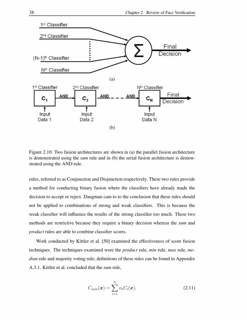
38 Chapter 2. Review of Face Verification
(a)
(b)
Figure 2.10: Two fusion architectures are shown in (a) the parallel fusion architectureis demonstrated using the sum rule and in (b) the serial fusion architecture is demon-strated using the AND rule.
rules, referred to as Conjunction and Disjunction respectively. These two rules provide
a method for conducting binary fusion where the classifiers have already made the
decision to accept or reject. Daugman cam to to the conclusion that these rules should
not be applied to combinations of strong and weak classifiers. This is because the
weak classifier will influence the results of the strong classifier too much. These two
methods are restrictive because they require a binary decision whereas the sum and
product rules are able to combine classifier scores.
Work conducted by Kittler et al. [50] examined the effectiveness of score fusion
techniques. The techniques examined were the product rule, min rule, max rule, me-
dian rule and majority voting rule; definitions of these rules can be found in Appendix
A.3.1. Kittler et al. concluded that the sum rule,
Csum(x) =
N∑
i=1
αiCi(x), (2.11)

2.4. Multi-Modal Person Verification 39
outperforms the other classifier combinations; where x is the feature vector, αi is the
ith weight and Ci is the ith classifier. This result was attributed to the fact that the
method is more resilient to estimation errors. When applying the sum rule the optimal
weights for fusion should be derived.
Several methods have been proposed for deriving the weights for classifier fusion.
Four methods were proposed by Benediktsson [11]:
• using equal weights (αi = 1N
),
• deriving weights based on ranking,
• dynamically weight by using a self rating scheme, and
• using heuristic methods to derive weights.
Another idea proposed by Benediktsson in [10] was to derive weights, not only for
each data source but also for each class. Often in pattern recognition literature few
details are given with regards to how weights for fusion are derived.
A general method for deriving fusion weights is to apply linear logistic regression
(llr). Unlike other methods such as linear regression or empirically deriving weights
this method is ensured to converge to a particular solution. Because the llr cost func-
tion,
Cllr =P
K
K∑
j=1
log(1 + e−fi−logit P )
+1 − P
L
L∑
j=1
log(1 + egj+logit P ), (2.12)
is convex it will converge to a solution. Where K is the number of true trials, L is the
number of false trials, P is the synthetic prior (which by default is P = 0.5), the fused
true scores,
fi = α0 +
N∑
i=1
αisij, (2.13)
fused false scores,

40 Chapter 2. Review of Face Verification
gi = α0 +N
∑
i=1
αirij, (2.14)
and the logit function is
logitP = logP
1 − P. (2.15)
An implementation of this method is provided by Brummer [22] as a fusion toolkit.
Within this toolkit is another method for deriving fusion weights the linear minimum
mean squared error (lm-MSE).
Brummer [22] noted that the minimisation of the lm-MSE method does not lead
to a convex function. As such one of the problems with using the lm-MSE method
is that the solution may lead to local minimal which are sub-optimal. For this reason
Brummer proposed that the lm-MSE method should be provided with starting weights
obtained using llr. The lm-MSE cost function,
CBrier =P
K
K∑
j=1
(1 − logit−1(fi + logit P ))2
+1 − P
L
L∑
j=1
(1 − logit−1(−gi − logit P ))2. (2.16)
is similar to the llr cost function. These methods for fusion have been applied to
multiple algorithms to improve speaker verification [22].
Several modalities have been examined to perform multi-modal person authentica-
tion. The prevalent methods include:
• 2D face images,
• fingerprints, and
• voice.
Jain et al. [47] noted that a major consideration for any multi-modal system is the
applicability of each modality. For instance if a system captures fingerprints it is fairly
easy to also capture a 2D face image, however, it may be much more difficult to capture

2.4. Multi-Modal Person Verification 41
a recording of their voice. An area of growing research interest is the use of 2D and 3D
face images for verification, also referred to as multi-modal face verification. Multi-
modal face verification is discussed in depth in the following section.
2.4.1 Multi-Modal Face Verification
Until recently face verification has only been considered as a uni-modal task often
using just the texture, or image (2D) data; although some researchers have examined
the use of 3D data. In conducting a survey of 2D face recognition, Zhao et al. noted
that the face is a 3D object that is recognised using only 2D data [111]. Given that
information about both modalities is available researchers have examined methods for
combining this information.
Fusion of the 2D and 3D modalities for face verification is receiving greater atten-
tion as it has thus far proven to be a more effective method than using either modality
on its own. Multi-modal face verification combines complementary information ob-
tained from different sensors. For instance the data captured using a laser scanner (3D
data) is quite different to that captured by a camera (2D data). The complementary
nature of the 2D and 3D modalities means that the weaknesses from any one modality
can be reduced. In a review of 3D FRTs Bowyer mentions some of the methods for
performing multi-modal face verification [20].
Combining the 2D and 3D modalities for face verification is a concept that has only
recently gained momentum. In 2001 Beumier and Acheroy [12] proposed a multi-
modal system which used the profiles of 3D and 2D face data. The scores from these
methods were then summed together using weights (weighted sum rule) with few de-
tails given as to how these weights are obtained.
In 2002 Wang et al. [103] proposed the use of two feature extraction technique and
performed feature fusion. Point signatures were used to feature from the 3D modality
and Gabor filters at fiducial points were used to obtain features from the 2D modality.
There were four fiducial points defined for the 3D face data and ten fiducial points de-
fined for the 2D face data. It was found that the combination of these features improved
performance and that the best performance was obtained when using an SVM. Us-
ing the same feature extraction techniques Wang et al. also examined classifier fusion

42 Chapter 2. Review of Face Verification
[101]. In this case a Hausdorff distance was used for each modality and it was shown
that weighting the combination of these two classifiers outperformed either classifier
on its own.
In 2003 Chang et al. [24] applied eigenfaces to both the 2D and 3D face data. A
system was defined for both the 2D and 3D face modalities and the scores were then
combined. The task was defined to be identification and so a combined Rank score
was obtained by fusing the Rank 1, Rank 2 and Rank 3 scores.
A technique using log-Gabor features on 2D and 3D part face images was described
by Cook et al. in [28]. The log-Gabor features were reduced with PCA and the 2D
and 3D classifiers were combined with equal weighted fusion. Despite the ongoing re-
search into hybrid 2D and 3D face recognition, work into combining feature modelling
techniques for 2D and 3D face recognition remains unaddressed. Further work in [29]
proposed the use of SVMs to derive the linear weights based on the discriminatory
measures defined by the SVM.
Work conducted by BenAbdelkader and Griffin [9] in 2004 examined the effective-
ness of multi-modal fusion for two algorithms: fisherfaces and a commercial system
by FaceIt [1] which is based upon LFA. The fusion scheme used when applying fish-
erfaces was a pixel-level fusion method, while for the FaceIt method the scores from
each classifier were combined using weighted summation. It was found that for both
algorithms multi-modal fusion led to an improved system, over using either the 2D or
3D face data. The best performing system, the FaceIt algorithm, had an accuracy of
100%. It was noted that the database being used consisted of 185 IDs with four images
per ID (740 images in total) and so further testing needed to be conducted on a larger
dataset.

Chapter 3
Experimental Framework
3.1 Introduction
In the previous chapter it was mentioned that a standard database is important to con-
duct objective experiments. It is also important to have a consistent set of experiments
to objectively analyse the performance an approach. There are two issues that limit the
experiments used for this thesis, these being:
1. the use of multi-modal (2D and 3D) face data, and
2. the application of feature distribution modelling.
The use of multi-modal face data limited the number of databases available for
use. The largest multi-modal face database was captured as part of the FRGC [80].
This database consists of 4950 joint 2D and 3D face images of 557 individuals (IDs).
However, the experiments defined for this database do not facilitate the application of
feature distribution modelling.
The experiments defined for the FRGC do not easily allow for the use of feature
distribution modelling. For instance the training set consists of 943 images and most
of the experiments are defined to use just one enrolment image [80]. For this reason
an alternate set of experiments were required which allowed for multiple enrolment
images and a larger training set.
The experimental framework defined in this chapter addresses two issues:
43

44 Chapter 3. Experimental Framework
1. having sufficient observations to perform feature distribution modelling, and
2. having sufficient test cases to derive meaningful results.
These two issues cannot be considered in isolation as they are both constrained by the
limited number of observations available from the FRGC database.
In the following section a description of the FRGC database is described followed
by an outline of the normalisation procedure. The experimental framework is then
defined and finally the performance measures used to present results in this thesis are
outlined.
3.2 Database Description
As previously mentioned, the FRGC database is used to conduct these experiments.
This database consists of 4950 joint 2D and 3D images of 557 IDs and was captured
over a one and a half year period, using a Minolta Vivid 910. This database is one of
the largest multi-modal face databases and consists of three sessions of data.
The three sessions were captured in the Spring of 2003, the Fall of 2003 and
the Spring of 2004. From hereon these data sets will be referred to as Spring2003,
Fall2003 and Spring2004. The Spring2003 session consists of 943 joint images of 275
IDs, while the Fall2003 session consists of 1893 joint images of 369 IDs. Finally, the
Spring2004 session consists of 2114 joint images of 346 IDs. The time lag between
each joint image capture is at least one week.
The collection of this database meant that there are a different number of images
captured for each ID. This has resulted in an interesting distribution of image captures,
for each ID in each session. The distribution of IDs with x number of images is pro-
vided in Figure 3.1. It can be seen that for the Spring2003 session there are one and a
half to two times the number of IDs with only one enrolment image when compared to
Fall2003 or Spring2004. This greatly reduces the number of IDs that can be enrolled
if only Spring2003 data is used for enrolment.
The Konica Minolta Vivid 910 [69] captures the 3D and registered 2D data as pro-
gressive scans. The 3D data is captured using a laser light and the 2D data is captured

3.2. Database Description 45
5 10 15 20 25 3010
10
20
30
40
50
60
70
80Entire FRGC Database
Number of Images
Num
ber o
f ID
s w
ith x
Num
ber o
f Im
ages
(a)
1 2 3 4 5 6 7 80
10
20
30
40
50
60
70
80FRGC Database − Spring2003
Number of Images
Num
ber o
f ID
s w
ith x
Num
ber o
f Im
ages
(b)
1 2 3 4 5 6 7 8 9 100
5
10
15
20
25
30
35
40
45
50FRGC Database − Fall2003
Num
ber o
f ID
s w
ith x
Num
ber o
f Im
ages
Number of Images
(c)
1 2 3 4 5 6 7 8 9 10 11 12 0
5
10
15
20
25
30
35
40
45FRGC Database − Spring2004
Number of Images
Num
ber o
f ID
s w
ith x
Num
ber o
f Im
ages
(d)
Figure 3.1: The distribution of IDs with a certain number of images are presented forseveral of the FRGC database configurations. In (a) the distribution is shown acrossthe entire database, (b) for Spring2003, (c) for Fall2003 and (d) for Spring2004.

46 Chapter 3. Experimental Framework
sequentially such that each channel (Red, Green and Blue) is captured separately. The
3D images take approximately 2.5 seconds to capture whereas the 2D images take ap-
proximately 0.5 seconds to be captured. All the data, 2D and 3D, is captured using the
same image sensor and so is pixel-wise registered.
The FRGC database was captured with challenging environmental conditions. The
most challenging environmental condition is the highly variant illumination. The illu-
mination conditions vary from overexposed images through to images with shadowing
across parts of the face. The environment conditions are particularly variant between
Spring2003 and the other two data sets, Fall2003 and Spring2004.
The images captured for the Spring2003 dataset are significantly brighter, and in
some cases are overexposed (see Figure 3.2). The images captured for the Fall2003 and
Spring2004 datasets are both captured under darker illumination conditions. However,
for the Fall2003 and Spring2004 data sets, there is significant illumination variation
across the face. For instance there are images which have significant shadowing across
the face, an example of this is provided in Figure 3.3.
Figure 3.2: A 2D image from the Spring2003 session which highlights the bright illu-mination. There are several regions which are saturated or overexposed.
Aside from visual inspection, the mean and standard deviation of the pixel val-
ues in each session, Spring2003, Fall2003 and Spring2004 were taken. These results
are presented in Table 3.1 and it can be seen that there is approximately a 100 pixel
intensity offset from Spring2003 to either Fall2003 or Spring2004.

3.3. Data Normalisation 47
(a) (b)
Figure 3.3: These images are indicative of the the varying illumination conditions inthe Fall2003 and Spring2004 sessions. In (a) the illumination is consistent across theentire face, whereas the illumination in (b) is significantly darker and varies across theface.
Spring2003 Fall2003 Spring2004
Mean Intensity 176.96 71.91 64.18
Std. Dev. 14.21 17.47 17.63
Table 3.1: The mean and standard deviation of the pixel intensity values forSpring2003, Fall2003 and Spring2004 images.
3.3 Data Normalisation
Data normalisation is an integral step for any pattern recognition problem. For face
verification, several methods have been proposed for conducting image normalisation.
A method for normalising 2D face data to provide illumination invariance was pro-
posed by Gross and Brajovic in 2003 [43]. Another method for 2D face normalisation
was proposed by Lowther et al. [57] in 2004 and was later used for 3D face normalisa-
tion by this author in 2005 [65]. Researchers at the Colorado State University (CSU)
also proposed a face normalisation procedure for both 2D and 3D data in 2003 [13].
The data normalisation process used for this work, is the same process that is used
for the baseline system of the FRGC. This consists of a CSU face normalisation proce-
dure [13] which applies a similar process to normalise both the 2D and 3D face data.
The normalisation process consists of the following steps: geometric normalisation,
masking, histogram equalisation and pixel normalisation. The geometric normalisa-
tion is said to line up the eyes, and the masking uses an elliptical mask to extract the

48 Chapter 3. Experimental Framework
face from the forehead to chin and cheek to cheek. Histogram equalisation normalises
the histograms of the extracted face region. Finally pixel normalisation ensures that
the face region has a mean of zero and standard deviation of one. An example output
of the CSU normalisation is provided in Figure 3.4 (a) and (b).
The CSU normalisation produces face regions that are surrounded by a mask,
where each pixel of the mask is set to be 0. Although this mask is consistent for
both the 2D and 3D images, the inclusion of a mask is not suited to some of the feature
extraction techniques examined in this work. This is because it will result in irregu-
larities at the boundary of the mask, and also for when the frequency response of the
entire image is taken.
This research examines the issues of holistic and local feature distribution mod-
elling, and one of the methods for feature extraction is the 2D-DCT. If portions of the
mask are included when applying the 2D-DCT then the mask will influence the result-
ing feature vector. The manner in which the mask will influence the feature vector will
be variable from image to image which is a highly undesirable trait.
To ensure the masked regions did not have any impact a cropped region of the
face was extracted. This cropped region was chosen so that the most salient features,
including the eyes and nose, were retained. The final region consisted of 108 × 108
pixels from the CSU normalised data. An example of this cropping, for the 2D and 3D
modality, is provided in Figure 3.4 (c) and (d).
3.4 Experimental Design
The experiments were designed around the following research questions:
1. Is it worthwhile to perform feature distribution modelling on holistic difference
vectors?
2. Is local feature distribution modelling an effective method of face verification
for the 3D modality? and
3. Does the multi-modal fusion of feature distribution modelling systems yield an
improved classifier?

3.4. Experimental Design 49
(a) (b)
(c) (d)
Figure 3.4: Examples of both 2D and 3D images when using the CSU algorithm arepresented. In (a) there is a normalised 2D face image and (b) there is a normalised 3Dface image while in (c) there is a cropped 2D face image and in (d) there is a cropped3D face image.

50 Chapter 3. Experimental Framework
The first and second questions, regarding feature modelling (of holistic and local vec-
tors), require multiple enrolment images to effectively train client specific models. The
third question of classifier score fusion means that the experiments have to retain the
correspondence between 2D and 3D images.
Multiple enrolment images are required to facilitate feature distribution modelling.
When performing feature distribution modelling client specific models are often de-
rived, in order to achieve this multiple observations of each client are required. Face
verification protocols have several images available to enrol a client for instance the
BANCA protocol [5] has five enrolment images per client and the XM2VTS protocol
I and II have three and four possible enrolment images respectively [68]. Upon further
examination of the distribution of images per ID, it was considered reasonable to set
the number of enrolment images to E = 4.
An issue that is considered of importance is cross-session variation, as this allows
any data dependencies to be examined. Cross-session tests enrol IDs from one session
and then test these IDs using the remaining sessions. Cross-session variation tests are
considered useful for several reasons. They indicate if the training or tuning is general
across data sets. They also indicate if there are capture conditions that can adversely
affect performance such as pose, illumination and expression variations.
The following sections outline the methods for splitting the data and for conduct-
ing performance evaluation. The data split defines all the cross-session variation ex-
periments and how various parameters, such as optimal dimensionality are derived.
Following this, the criteria for performance evaluation are defined and explained.
3.4.1 Data Split
Any data split used for this thesis needs to address the following points:
• the correspondence between the joint 2D and 3D images has to be retained,
• cross-session variation needs to be examined,
• an independent set has to be defined to derive tuning parameters, and
• enough data must be available to perform feature distribution modelling.

3.4. Experimental Design 51
For this thesis, the data was split so that cross-validation experiments could be con-
ducted. This is not to be confused with tests which examine cross-session variation.
Cross-session variation consists of enrolling an ID in one session, and then test-
ing on the remaining session; the merits of this analysis have already been discussed.
There are three separate capture sessions in the FRGC data Spring2003, Fall2003 and
Spring2004. These sessions are used to define four distinct sessions, Spring2003,
Fall2003, Spring2004 and All. The All session is formed by pooling all the data from
Spring2003, Fall2003 and Spring2004. Experiments conducted using the All session
make no assumption as to the database conditions. The other sessions, Spring2003,
Fall2003 and Spring2004, are used to examine cross-session variability. For instance,
when using the Spring2003 session, the IDs are enrolled using data from Spring2003
and then tested using data from the other sessions Fall2003 and Spring2004.
On the other hand, cross-validation experiments change the combination of train
and test data to ensure that the results obtained are consistent. For these experiments,
there are three disjoint sets the Train, Tune and Test sets, and so the data that comprises
these sets is changed so that it can be shown that the results are consistent. The data
for these three disjoint sets is split with a ratio of 2:1:1 between Train, Tune and Test
respectively.
The method chosen for dividing the database between the Train, Tune and Test
sets was to define four disjoint splits. The data is evenly, and randomly, divided into
four splits which are disjoint based on the IDs. Using these splits the cross-validation
experiments were defined. This means that the Train, Tune and Test sets are formed
by changing which split is assigned to which task. For instance, in Figure 3.5 training
is conducted using set1 and sett2. Tuning is conducted using set3 and then testing is
conducted on set4. For each Train set the Tune and Test sets are separate. A new Train
set is then formed by using split2 and split3 to conduct training, and using set4 and
set1 for tuning and testing.
These Train, Tune and Test sets are used in the following manner, the:
Train set is used to conduct training such as deriving the PCA space, world GMMs
and as background data. No assumptions are made regarding session or database
conditions when using this data.

52 Chapter 3. Experimental Framework
Figure 3.5: An example of the division for the Train, Test and Tune sets.
Tune set is used to determine the optimal parameters for the systems. This includes
determining the optimal dimensionality for PCA. As with the Train set no as-
sumptions are made regarding session or database conditions when using this
data.
Test set is used to conduct the testing of the systems. Several different tests are con-
ducted including, tests that analyse cross-session variation. Cross-session vari-
ation consists of enrolling the data using one session and then testing using the
remaining sessions. Therefore the database conditions between the enrolment
and test images can be mismatched.
The Train set uses data from the All session, using all available data from
Spring2003, Fall2003 and Spring2004. This set is used to derive the PCA space, global
IP GMM and for background data to train client specific EP GMMs. In this work four
different Train sets are used: (set1, set2), (set2, set3), (set3, set4) and (set4, set1)
(this notation is shortened to shuffle12, which refers to using (set1, set2) to conduct
training). The four different Train sets are chosen so that each set (set, set2, set3 and
set4) is used once for testing.
The Tune set is used to derive optimal parameters such as fusion weights, dimen-
sionality and number of mixture components. To derive these parameters the All ses-
sion is used, in the same manner as the All session of the Test set. This is done to ensure
that optimisation is conducted making no assumptions regarding database conditions.
There are four Tune sets set3, set4, set1 and set2.
The Test set makes use of the four sessions: All, Spring2003, Fall2003 and
Spring2004. When performing tests upon the All session, enrolment data is taken

3.4. Experimental Design 53
randomly and the remaining data is then used to form the test lists. The remaining ses-
sions (Spring2003, Fall2003 and Spring2004) are used to analyse cross-session varia-
tion. For the cross-session experiments enrolment data is taken from a session and only
data from the sessions is used to conduct tests. For instance, tests on the Spring2003
session data from Spring2003 is randomly selected to enrol clients and all the data
from the remaining sessions, Fall2003 and Spring2004, are used for testing. There are
four Test sets with each split being used once for testing set4, set1, set2 and set3.
3.4.2 Performance Evaluation
Performance evaluation methods are integral for analysing any system. An important
issue for performance evaluation is to have an appropriate reference, or baseline sys-
tem, to compare against. The choice of performance criteria is also important. For
verification systems two groups of errors provide a concise description of the system:
• the false alarm rate (FAR), and
• the false rejection rate (FRR).
The FAR refers to the number of times an input is accepted when it shouldn’t be. For
example, if ID5 claims to be ID4 and this is accepted as the truth, then it is a false
acceptance error. The FRR refers to the number of times that an input is rejected when
it shouldn’t be. An example of this would be when ID5 claims to be ID5 and this is
not accepted as the truth, this is a false rejection error. These two groups of errors can
be used to describe the performance of a system.
Many methods have been proposed for comparing the performance of verification
systems. These include comparing particular operating points and examining plots
which describe a system’s performance characteristics. For this work the following
methods are used to present results:
1. Concise results are presented for three operating points:
(a) The FAR at 0.1%; this operating point is the operating point of most inter-
est.

54 Chapter 3. Experimental Framework
(b) The FAR at 1.0%.
(c) The equal error rate (EER), which is where FAR = FRR.
2. A detailed description of a system is presented using a detection error tradeoff
(DET) plot.
The operating points of interest in this work are based on the progression of oper-
ating points used for several evaluations. The main operating point, FAR = 0.1%, is
chosen because it is the current operating point of interest for the recent FRGC [80];
for both 2D and 3D modalities. In previous evaluations, such as the FRVT 2002, an
operating point of FAR = 1% was chosen and so where appropriate this operating
point is also presented. The final operating point, the EER, is presented to provide
a more complete description of system performance. It is also an operating point that
has been used in face verification competitions [66, 67]
The most complete method for comparing verification systems is to provide a plot
of its performance characteristics. The two most common plots of system performance
are the Receiver Operating Characteristics (ROC) and the Detection Error Tradeoff
(DET). The ROC plots describe the percentage of FAR versus the percentage of (1 −FAR), with both values plotted on linear scales. These plots have been used to fully
describe systems as part of the FRGC [80].
The DET plots describe the percentage of FAR versus the percentage of FRR,
however, these are both plotted on log scales. They provide a description of the system
performance that is usually linear, thereby making interpretation of the results easier.
This method has been used as part of the speaker recognition evaluations conducted
by the National Institute of Standards and Technology (NIST) [64, 35]. The use of the
DET curve for assessing system performance was described by Martin et al. in [63].
For both methods of presentation two sets of values can be presented because cross-
validation experiments are being conducted. By using cross-validation experiments,
results can be presented based on the performance of the separate Test sets or by pool-
ing the results from all the Test sets. In this work the results are presented using only
the pooled result this is because the low number of trials for each separate Test set
makes the individual results less meaningful. Pooling the results consists of collating

3.4. Experimental Design 55
the classifier results for each test and then deriving the performance characteristics. So
the classifiers results for the All tests on set1, set2, set3 and set4 are pooled together
and used to derive the performance characteristics for the All tests.

56 Chapter 3. Experimental Framework

Chapter 4
Holistic Feature Extraction
4.1 Introduction
Initial face recognition research used local features to recognise the human face, see
Chapter 2 for details. However, in the past 15 years, holistic feature extraction has
risen in prominence. One of the first fully automatic face recognition systems by Turk
and Pentland [98] used holistic features to perform verification, referred to as eigen-
faces. This holistic feature extraction technique has since become a de facto standard
of the face verification community, as was shown by the fact that it formed the baseline
system for the FRGC [80].
Holistic feature extraction techniques often compare the representations of two
faces using distance- or angular-based measures. For instance, there has been a pro-
gression of research examining the optimal similarity measure for the eigenfaces tech-
nique. In 1998, Moon et al. [72] reviewed several similarity measures, this work was
furthered in 2000 by Yambor et al [107] who found a Mahalanobis angle measure
performed best. More recently, in 2003, Bolme et al. [18] noted that the MahCosine
measure provided the best performance. This last similarity measure has been used
with the eigenfaces technique to form the baseline system of the recent FRGC [80].
In this chapter, the baseline verification system used in the remainder of this the-
sis is defined. This system extracts holistic features by applying the eigenfaces tech-
nique. These holistic features are compared using the MahCosine similarity measure,
57

58 Chapter 4. Holistic Feature Extraction
an angular-based measure. A second holistic feature extraction technique, the 2D-
DCT, is also examined.
The performance of holistic 2D-DCT features are examined because these features
are used in the following chapter. In the next chapter 2D-DCT features are used to
perform holistic feature distribution modelling. Therefore the relative performance of
these features using distance- and angular-based measures had to be investigated.
4.2 Feature Extraction Techniques
The two techniques for holistic feature extraction examined in this work are, eigenfaces
and the 2D-DCT. The eigenfaces technique is a specific application of PCA and from
hereon will be referred to as PCA. This method has become a de facto standard of the
face verification community, for instance it was used to as the baseline system for the
recent FRGC [80]. The 2D-DCT as a method for holistic feature extraction is rarely
used in face verification. This is because it provides a sub-optimal representation of
the face; no training is conducted as it is a pre-defined linear transform. As such it is
concluded that comparing 2D-DCT features using distance- or angular-based measures
should not result in a useful classifier, a result which initial experiments support.
PCA was first applied to face verification by Turk and Pentland in 1991 [98]. This
technique works by applying eigen decomposition to the covariance matrix of a set of
training vectors (vectorised training images). The covariance matrix is formed from the
M mean normalised column vectors x, which in this case are the vectorised training
images. The covariance matrix,
C =1
M
M∑
i=1
xT x, (4.1)
has eigen decomposition applied and the resulting eigenvectors are ranked in descend-
ing order of their eigenvalue λi (the ith eigenvalue). The D most relevant eigenvectors
are then retained to define a sub-space Φ such that D << N 2; the images are consid-
ered to be of size N × N and so result in vectors of size N 2. An vectorised image can
then be projected into this vector space to produce a D dimensional feature vector a.

4.2. Feature Extraction Techniques 59
Several methods have been proposed to compare the feature vectors obtained
through PCA. Bolme et al. [18] concluded that the MahCosine measure,
d(u, v) =u.v
|u||v| , (4.2)
provided the best performance for PCA feature vectors. This is a Mahalanobis based
similarity measure as it measures the cosine angle between two vectors and also uses
the covariance matrix. Because the covariance matrix is diagonalised (due to PCA) the
covariance matrix can be introduced to the similarity measure by normalising the PCA
feature vectors based on the eigenvalue (or variance) of the eigenvector such that,
u =
[
x1√λ1
,x2√λ2
, ...,xi√λi
]
and (4.3)
v =
[
y1√λ1
,y2√λ2
, ...,yi√λi
]
. (4.4)
This similarity measure has recently become the standard method used for PCA feature
vectors as shown by its use in the FRGC evaluation.
Holistic 2D-DCT features are investigated because they are used for feature dis-
tribution modelling in the following chapter. Therefore the relative performance of
these features using distance- or angular-based measures had to be considered. Holis-
tic 2D-DCT features have previously been by Pan et al. [78] to derive a neural network
verification system. However, limited research has been conducted using holistic 2D-
DCT features and similarity measures to perform face verification.
The 2D-DCT is a pre-defined linear transform that encodes an image based on its
frequency content. The transform,
F (u, v) =
√
2
N
√
2
M
N−1∑
x=0
M−1∑
y=0
Λ(x)Λ(y)β(u, v, x, y)I(x, y), (4.5)
is applied to a N × M image I(x, y) where
β(u, v, x, y) = cos[π.u
2N(2x + 1)
]
cos[ π.v
2M(2y + 1)
]
(4.6)
and

60 Chapter 4. Holistic Feature Extraction
Λ(ε) =
1√
2for ε = 0
1 otherwise
. (4.7)
This transform produces as many coefficients as there are input pixels; for an N × N
image there are N 2 2D-DCT coefficients (see Appendix A.2 for more details). To use
these coefficients for face verification dimensionality reduction needs to be performed
such that D << N 2.
A common method for reducing the dimensionality of a 2D-DCT feature vector
is to retain the low frequency coefficients. The JPEGG2000 standard [2] ranks the
2D-DCT coefficients based on their ascending frequency content by applying a zig-
zag pattern, see Figure 4.1. In this figure the coefficients are numbered from 0, as
the 0th coefficient represents the average value, or DC component. Another method
for reducing the dimensionality is to retain those coefficients which best represent the
face.
Figure 4.1: An example of the JPEG zig-zag ordering of 2D-DCT coefficients for animage of size 4 × 4.
By retaining the most variant coefficients, across a set of training images, the error
in reconstruction can be minimised. This is similar to PCA, however, unlike PCA the
basis functions relate to a frequency component. These variance ranked coefficients al-
low for the application of a similarity measure such as the MahCosine measure, which
was shown to be advantageous for PCA.
The variance ranked 2D-CT coefficients are determined from a set of training im-
ages. The mean of the training set,

4.2. Feature Extraction Techniques 61
Ψf =1
N
N∑
i=1
f i, (4.8)
is subtracted from each training vector. These normalised vectors,
f i = f i − Ψf , (4.9)
are used to calculate the variance for each coefficient and the 2D-DCT coefficients are
then reordered in descending order of their variance σ2DCT,i.
Initial experiments in this thesis showed that holistic 2D-DCT features performed
significantly worse than PCA. Using holistic 2D-DCT features it was found that the
MahCosine similarity measure provided the best results. Comparing the performance
of this holistic 2D-DCT verification system was a holistic PCA verification system, it
was was found that the PCA system performed significantly better (see Figure 4.2).
Therefore further investigation into a face verification using holistic 2D-DCT features
using distance- or angular-based measures was not pursued further.
0 500 1000 1500 2000 250010
15
20
25
30
35
40
45
50
55
60
Dimensions (D)
FAR
= 0
.1%
3D Modality
PCA
2D−DCT
Figure 4.2: A plot of the FRR at FAR = 0.1% for two 3D face verification systems.One verification system uses PCA features and the other verification system uses 2D-DCT features; both systems use the MahCosine similarity measure.
In the following section the baseline verification system is described for both the
2D and 3D modalities. This verification system is used throughout the remainder of
this thesis and uses PCA to obtain the holistic features. The MahCosine measure is

62 Chapter 4. Holistic Feature Extraction
used to compare the holistic features as it was concluded by Bolme et al. [18] to provide
the best performance.
4.3 Baseline System
In order to perform an evaluation a reasonable baseline verification system needs to
defined. For this thesis the baseline verification system, for both the 2D and 3D modal-
ities, uses PCA for feature extraction. This feature extraction technique was chosen as
it is ubiquitous in face verification literature and is one of the most researched face
verification techniques. The PCA feature vectors are compared using the MahCosine
similarity measure, as it was concluded by Bolme et al. [18] to be the optimal similarity
measure.
The baseline verification system uses cropped face images and has multiple en-
rolment vectors to use in the verification process. Cropped images are used for this
system because the experiments in the remainder of this thesis are conducted on the
cropped images; the reasons for this are outlined in Section 3.3. The issue of multiple
enrolment images stems from the fact that they are needed to perform effective feature
modelling. It was found that averaging these scores,
Cmean(X, y) =1
E
E∑
i=1
CMahCosine(xi, y), (4.10)
provided the best performance. Note that X is the set of enrolment vectors, xi is the
ith enrolment vector, y is the test vector and E is the number of enrolment vectors.
To fully define the baseline verification system two issues need to be addressed,
the:
1. optimal number of dimensions D to retain, and
2. comparative performance between full face images and cropped image.
The number of dimensions was varied, D = [50, 100, 150, ..., 2300], and the system
that performed best at the FAR = 0.1% was chosen. This operating point was chosen
as it was the operating point of interest in the recent FRGC evaluation; see Section 3.4.2
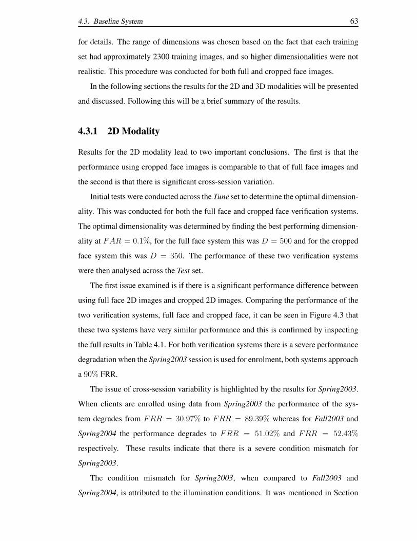
4.3. Baseline System 63
for details. The range of dimensions was chosen based on the fact that each training
set had approximately 2300 training images, and so higher dimensionalities were not
realistic. This procedure was conducted for both full and cropped face images.
In the following sections the results for the 2D and 3D modalities will be presented
and discussed. Following this will be a brief summary of the results.
4.3.1 2D Modality
Results for the 2D modality lead to two important conclusions. The first is that the
performance using cropped face images is comparable to that of full face images and
the second is that there is significant cross-session variation.
Initial tests were conducted across the Tune set to determine the optimal dimension-
ality. This was conducted for both the full face and cropped face verification systems.
The optimal dimensionality was determined by finding the best performing dimension-
ality at FAR = 0.1%, for the full face system this was D = 500 and for the cropped
face system this was D = 350. The performance of these two verification systems
were then analysed across the Test set.
The first issue examined is if there is a significant performance difference between
using full face 2D images and cropped 2D images. Comparing the performance of the
two verification systems, full face and cropped face, it can be seen in Figure 4.3 that
these two systems have very similar performance and this is confirmed by inspecting
the full results in Table 4.1. For both verification systems there is a severe performance
degradation when the Spring2003 session is used for enrolment, both systems approach
a 90% FRR.
The issue of cross-session variability is highlighted by the results for Spring2003.
When clients are enrolled using data from Spring2003 the performance of the sys-
tem degrades from FRR = 30.97% to FRR = 89.39% whereas for Fall2003 and
Spring2004 the performance degrades to FRR = 51.02% and FRR = 52.43%
respectively. These results indicate that there is a severe condition mismatch for
Spring2003.
The condition mismatch for Spring2003, when compared to Fall2003 and
Spring2004, is attributed to the illumination conditions. It was mentioned in Section

64 Chapter 4. Holistic Feature Extraction
All Spring2003 Fall2003 Spring2004Cropped FAR = FRR 7.22% 31.62% 15.32% 19.80%
Face FAR = 1 16.53% 76.87% 34.85% 40.99%
FAR = 0.1 30.97% 89.39% 51.02% 52.43%
Full FAR = FRR 6.14% 31.28% 13.96% 18.82%
Face FAR = 1 14.28% 79.11% 32.92% 40.07%
FAR = 0.1 29.11% 89.83% 49.55% 52.83%
Table 4.1: The performance using Cropped and Full 2D face images is presented usingthree operating points, FAR = FRR, FAR = 1 and FAR = 0.1.
All Spring2003 Fall2003 Spring20040
10
20
30
40
50
60
70
80
90
Session
FRR
at F
AR
=0.1
%
Full Face vs Cropped Face
Full FaceCropped Face
Figure 4.3: A bar graph showing the performance of the PCA MahCosine classifierusing full face 2D images and cropped 2D images at FAR = 0.1%.
3.2 that several images within Spring2003 were in fact saturated, and that the gen-
eral illumination was quite bright. By comparison, the illumination for the Fall2003
and Spring2004 sessions is much darker, although for these two sessions there can be
significant shadowing across the face.
Another issue addressed within these tests is to examine the distribution of the PCA
features. The distribution of each dimension was examined to determine if a measure
that uses more than just the second order statistics is suitable; the Mahalanobis cosine
measure makes use of some information from the variance, or the second order statis-
tic, of each dimension. The D’Agostino Pearson’s test for normality [95] was applied

4.3. Baseline System 65
to each dimension of the feature vectors from the Train set. It was found that 88.71% of
the retained dimensions (D = 350) were not normal distributions with a significance
level of 0.05. The following question is then considered, since there is more to the
distribution of each dimension than a Gaussian distribution (defined by first and sec-
ond order statistics, the mean and covariance) is there a better method of performing
verification than the MahCosine measure, which uses at most the covariance (second
order statistics) to compare the feature vectors? One possible method is to model the
distribution of the holistic features and this is the basis for the work conducted in the
following chapter.
4.3.2 3D Modality
Results for the 3D modality lead to two important conclusions. The first is that the
performance using cropped face images is comparable to that of full face images and
the second is that there is limited cross-session variation. Before conducting these
experiments the optimal dimensionality for each system was determined.
The optimal number of dimensions for the full face system and the cropped face
system was determined by analysing the performance on the Tune sets. The system
which performed best at FAR = 0.1% on the Tune sets was chosen as the optimal
system. For the full face system this led to D = 550 while the cropped face system
D = 150. The performance of these optimal systems was then analysed on the Test
sets.
The results for the 3D modality show that there is little difference in performance
when using full or cropped face images. Results for the 3D modality, provided in
Table 4.2, show that the performance of the full face and cropped face systems is
similar. This result is further highlighted by examining the plots of the performance
at FAR = 0.1%, see Figure 4.4. These results also highlight that there is limited
cross-session variability for the 3D modality.
The results for cross-session variation show that there is limited cross-session vari-
ability, this result is attributed to two facts. First, the 3D data is inherently robust to
illumination variations, which adversely effects the 2D modality. Second, the 3D data
is captured at a high resolution, Phillips et al. [80] that the 3D data was captured at a
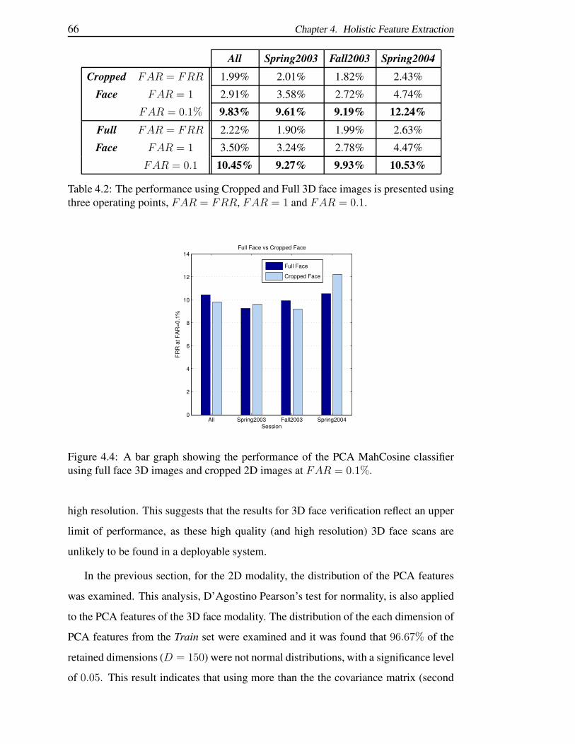
66 Chapter 4. Holistic Feature Extraction
All Spring2003 Fall2003 Spring2004Cropped FAR = FRR 1.99% 2.01% 1.82% 2.43%
Face FAR = 1 2.91% 3.58% 2.72% 4.74%
FAR = 0.1% 9.83% 9.61% 9.19% 12.24%Full FAR = FRR 2.22% 1.90% 1.99% 2.63%
Face FAR = 1 3.50% 3.24% 2.78% 4.47%
FAR = 0.1 10.45% 9.27% 9.93% 10.53%
Table 4.2: The performance using Cropped and Full 3D face images is presented usingthree operating points, FAR = FRR, FAR = 1 and FAR = 0.1.
All Spring2003 Fall2003 Spring20040
2
4
6
8
10
12
14Full Face vs Cropped Face
Session
FRR
at F
AR
=0.1
%
Full Face
Cropped Face
Figure 4.4: A bar graph showing the performance of the PCA MahCosine classifierusing full face 3D images and cropped 2D images at FAR = 0.1%.
high resolution. This suggests that the results for 3D face verification reflect an upper
limit of performance, as these high quality (and high resolution) 3D face scans are
unlikely to be found in a deployable system.
In the previous section, for the 2D modality, the distribution of the PCA features
was examined. This analysis, D’Agostino Pearson’s test for normality, is also applied
to the PCA features of the 3D face modality. The distribution of the each dimension of
PCA features from the Train set were examined and it was found that 96.67% of the
retained dimensions (D = 150) were not normal distributions, with a significance level
of 0.05. This result indicates that using more than the the covariance matrix (second

4.3. Baseline System 67
order statistics) may lead to improved verification.
4.3.3 Summary
Within this section the baseline verification system for the 2D and 3D modalities have
been defined. These verification systems use holistic PCA features from cropped face
images these PCA feature vectors are then compared using the MahCosine measure.
Cropped face images are used for all the methods examined in this thesis because the
full face images have a mask that can lead to irregularities for certain feature extraction
techniques; such as block based approaches.
Two key conclusions were made about the 2D and 3D baseline verification systems:
1. the performance of the cropped face (baseline) verification system is similar to
that of the full face verification system, and
2. the distribution of the PCA feature vectors might be better described by using
more than first and second order statistics.
The baseline verification system used for these experiments obtains holistic face
features by applying PCA to cropped face images. Experiments were conducted for
both modalities which showed that using cropped face images provides similar perfor-
mance to using full face images. This was an important finding as cropped face images
have to be used in later work because the mask present in the full face images will
cause irregularities in other techniques (see Section 3.3 for more details). Examining
the performance of the 2D and 3D baseline verification systems it was found that the
2D verification system had significantly degraded performance when there was session
variability.
Cross session variations were shown to adversely affect verification performance
for the 2D modality. The most extreme affect was found when clients were enrolled
using Spring2003 as the FRR approached 90% at a FAR = 0.1%. This perfor-
mance degradation is attributed to the extreme lighting variation between Spring2003
and the remaining sessions Fall2003 and Spring2004. The general illumination of the
Spring2003 session has approximately a 100 intensity offset, for an intensity range

68 Chapter 4. Holistic Feature Extraction
of 0 − 255. This susceptibility to session variations was not found for experiments
conducted on the 3D modality.
The experiments conducted for the 3D baseline verification system indicated that
its performance was superior to the 2D modality. The 3D baseline verification system
had superior performance across all Test conditions, an example of this is highlighted
in Figure 4.5. It was also found that 3D modality was robust to session variability with
the average FRR being 10.22% with a standard deviation of ±1.37% (for the four Test
conditions at FAR = 0.1%). The feature vectors used for the baseline verification
system for each modality were then examined and it was argued that a more complex
verification technique could be applied such as feature distribution modelling.
0.1 0.2 0.5 1 2 5 10 20 40
0.1
0.2
0.5
1
2
5
10
20
40
False Acceptance Rate (in %)
Fals
e R
ejec
tion
Rat
e (in
%)
Baseline Verification Systems
3D Modality
2D Modality
Figure 4.5: A DET plot comparing the performance of the 2D baseline verificationsystem versus the 3D baseline verification system. Results are presented by poolingthe data all the Test sets of the All session.
The baseline verification system uses the MahCosine measure to perform verifica-
tion. It’s noted that the MahCosine measure is an angular measure (based on the first
order statistics) that uses the covariance matrix (second order statistics) to compare
two feature vectors. For these experiments the second order statistics were obtained
by using the covariance matrix from PCA; which is a diagonalised covariance ma-
trix formed using the eigenvalues. Analysing the distribution of each PCA dimension
from the Train sets it was found that the majority of the retained dimensions were not
normal distributions, with a significance of 0.05. For the 2D modality 88.71% of the

4.3. Baseline System 69
retained dimensions (D = 350) were not normal and for the 3D modality 96.67% of
the dimensions (D = 150) were not normal. It is therefore proposed that a verification
system which used more than the second order statistics (the covariance matrix used
in the MahCosine measure) could improve verification performance. A more complex
representation for the holistic features is obtained by modelling their distribution. This
is the basis for the work conducted in the following chapter.

70 Chapter 4. Holistic Feature Extraction

Chapter 5
Holistic Feature Distribution
Modelling
5.1 Introduction
In the previous chapter a baseline verification system that used holistic PCA features
was described. This baseline verification system compares feature vectors using the
MahCosine measure, this is a measure that incorporates the covariance or second or-
der statistics. Analysing the distribution of the PCA feature vectors it was concluded
proposed a more complex representation (rather than using at most the second order
statistics) could provide improved verification; this conclusion was based on the fact
that the distribution of most of the dimensions were not normal.
One method for providing a more complete description of complex data is to per-
form feature modelling. Feature modelling describes the probability distribution func-
tion (pdf) of a data set. A commonly used method to perform feature modelling is
Gaussian Mixture Modelling. This method has been applied to other pattern recogni-
tion tasks such as speaker verification for over a decade [84]. For several pattern recog-
nition tasks feature modelling is better described as feature distribution modelling, as
it is the distribution of the feature that is being modelled.
Feature distribution modelling is rarely applied to the task of face verification be-
cause there is often insufficient data to perform modelling. A method for performing
holistic feature distribution modelling was proposed by Cook et al. [27] in 2004. In this
71

72 Chapter 5. Holistic Feature Distribution Modelling
work the registration error from the iterative closest point (ICP) algorithm was mod-
elled using GMMs. Other methods for feature distribution modelling have involved
breaking the face into parts and describing the distribution of these features [76, 90]
which is a form of local feature distribution modelling. The local methods for fea-
ture distribution modelling obtain extra observations by dividing the face into blocks
while the holistic method proposed by Cook et al. used a low number of dimensions
together with a low complexity model to describe this data; the largest GMM size was
six components.
In this chapter a novel approach to holistic feature distribution modelling is pro-
posed. It is proposed that extra observations of holistic feature vectors can be obtained
by forming the permutations of the holistic difference vectors. However, the number of
extra observations obtained with this technique are still insufficient to conduct client
specific feature distribution modelling. Therefore the difference vectors are used to
represent two forms of variation: Intra-Personal (IP) and Extra-Personal (EP). The IP
variation describes the variation that occurs between feature vectors from the same in-
dividual, while EP variation describes the variation that occurs between feature vectors
of different individuals. A novel method for combining these two models, the weighted
log-likelihood ratio, is then proposed and it shown that this leads to an improved veri-
fication system.
The remainder of this chapter is structured as follows. Feature distribution mod-
elling using GMMs is described, following this is an in depth discussion of difference
vector distribution modelling. The results of feature distribution modelling for two
holistic feature extraction techniques are then analysed. The work presented in this
chapter is then summarised.
5.2 Gaussian Mixture Models
Gaussian Mixture Modelling provides a compact framework for describing probability
density functions. This is concept is illustrated in Figure 5.1 where an observed proba-
bility density function (pdf) is fully described by a linear combination of M unimodal
Gaussians. This is a compact representation as each Gaussian is defined by only two

5.2. Gaussian Mixture Models 73
parameters, its mean (µ) and standard deviation (σ).
Set of Gaussians Representing a pdf
pdf to represent
Set ofGaussiansrepresentingthe pdf
Figure 5.1: A set of Gaussians used to model a probability density function (pdf).
The example provided in Figure 5.1 demonstrates the case for describing a single
dimension. Expanding this concept to the multi-dimensional case, the linear combina-
tion of M Gaussians is defined by,
p(x|λ) =
M∑
i=1
ωig(x|µi,Σi), (5.1)
where x is the test observation, µi is the mean vector of the ith mixture component
and Σi is the covariance matrix of the ith mixture component.
Each mixture component of the GMM is a single multi-dimensional Gaussian.
Therefore, µi is of length D × 1 and Σi is a D × D matrix. However, Σi is often
considered as a diagonalised matrix which greatly simplifies the problem of estimation
and scoring; this reduces the size of the covariance matrix from D2 to D. The term
g(x|µi,Σi),
g(x|µi,Σi) =1
√
(2π)D |Σi|exp
(
−1
2(x − µi)
′
Σ−1i (x − µi)
)
, (5.2)
represents a mixture component of the GMM. It is important to note that the weights
associated with each component, ωi, must sum to unity (∑M
i=1 ωi = 1) such that it
satisfies the requirement that the integral of a pdf equals unity.

74 Chapter 5. Holistic Feature Distribution Modelling
This method of feature modelling has previously been applied to face verification
by Sanderson and Paliwal [90]. Sanderson and Paliwal used GMMs to derive client
dependent models (C) using local features. This technique was extended by Sanderson
et al. [89] to include a client dependent background model (C) by using the LLR,
g(z) = `(z | C) − `(z | C), (5.3)
where z represents the feature vector to match, and `(z | C) is the average log like-
lihood score for class C. The use of GMMs, by Sanderson and Paliwal, was inspired
from its application in speaker verification. The use of GMMs was introduced to the
field of speaker verification in 1992 by Reynolds [84]. This method of feature mod-
elling has been further developed and used to generate some of the best performing
systems in the NIST speaker recognition evaluations [35].
5.3 Feature Distribution Modelling
Feature distribution modelling of holistic feature vectors is a difficult task due to the
limited number of training observations available. This is because there are a limited
number of images (observations) to perform training. The approach taken in this work
is to increase the number of observations available for training by performing feature
distribution modelling on difference vectors.
Holistic difference vectors have previously been used for face verification by
Moghaddam et al. [71, 70]. These difference vectors were used to define two
forms of variation Intra-Personal and Extra-Personal. The Intra-Personal (IP) varia-
tion described the variation that between images of the same individual and Extra-
Personal (EP) variation described the variation between images of different individ-
uals. Moghaddam et al. used these difference vectors to derive an IP sub-space and
an EP sub-space by applying PCA. The information from these sub-spaces was com-
bined in a Bayesian framework by using the covariance matrix from each sub-space;
this was used to define a Bayesian framework. This work conducted by Moghaddam
et al. makes the implicit assumption that the distribution of these difference vectors is
well described using just the second order order statistics; this would be the case if the

5.3. Feature Distribution Modelling 75
distribution of difference vectors was normal.
The novel work conducted in this thesis uses difference vectors in a different man-
ner. In this thesis it is assumed that the distribution of difference vectors are not normal
and therefore not well described using just the second order statistics. This means that
the difference vectors could be better described by using a more complex representa-
tion than the covariance matrix (second order statistics). The complex representation
considered in this thesis is to perform feature distribution modelling.
In the following sections the assumptions and properties of the IP and EP difference
vectors are presented and discussed. Included in this discussion are the methods that
can be used for forming the difference vectors.
5.3.1 IP Difference Vectors
The IP difference vectors,
∆IP = a − b, (5.4)
are used to described variation that occurs between images of the same individual; a
is the holistic features of image Ia and b is he holistic features of image Ib. Practical
limitations mean that there is rarely enough data to do this in a client specific manner.
An assumption made in this work is that the IP variation (IP feature space) is similar for
every person. In other words the differences between images of the same person are in
fact similar for all people; for instance minor pose variations, blinking, squinting and
other expressions are similar for all people. This assumption is supported by the fact
that Moghaddam et al. [71, 70] were able to derive a useful sub-space comprised only
of IP variation. This means that a global IP model, ΩIP , can be derived that describes
the IP variation for all individuals. By forming a global IP model all the IP difference
vectors are able to be used. This still leaves the question of which IP difference vectors
should used to derive ΩIP ?
There are two methods to form the IP difference vectors:
1. form all the combinations, or
2. form all the permutations.

76 Chapter 5. Holistic Feature Distribution Modelling
By forming all the combinations the number of observations (N ) available for training
is,
N =D
∑
i=1
niC2, (5.5)
whereas if the all the permutations are used,
N =
D∑
i=1
niP2. (5.6)
For both methods the IP difference vectors should have minimal variation; as it’s de-
scribing the variations between images of the same people. This means that,
∆IP ≈ 0, (5.7)
which was shown to provide good performance by Moon and Phillips [72], for holistic
PCA features.
The pros and cons of the two methods, forming the combination of difference vec-
tors and forming the permutation of difference vectors, are analysed in depth in the
following sections. It is shown that the most appropriate method of forming the differ-
ence vectors is to generate all the permutations.
Combination of Difference Vectors
If all the combinations of the IP difference vectors are used to derive ΩIP two issues
need to be addressed:
1. there is an implied correct method to subtract two feature vectors, and
2. the combination of IP difference vectors will likely form more positive, or neg-
ative, examples for each dimension.
When performing the combination of difference vectors only one of the two possible
combinations, (a − b) or (b − a), is used. Since,
(a − b) 6= (b − a), (5.8)

5.3. Feature Distribution Modelling 77
this means there’s an implied correct method to subtract two feature vectors. One
solution would be to take the absolute value of the IP difference vectors,
∆IP = ‖a − b‖. (5.9)
The second issue, of generating more positive, or negative, examples for each di-
mension leads to a skewed representation of the difference vectors. For example, if
the absolute value of the IP difference vectors is used, Equation 5.9, then only positive
examples are produced. Since feature modelling is achieved using GMMs, the derived
GMMs will be forced to represent only the positive region even though a GMM is a
continuous function.
Permutation of Difference Vectors
When using all the permutations of difference vectors to perform training the resultant
GMM should be odd symmetric. For instance the means of the derived GMMs should
be approximately the same for both the positive and negative part of the IP feature
space. This is because,
(a − b) = −(b − a), (5.10)
and also,
N∑
i=1
∆i,IP = 0. (5.11)
The number of observations available when using all the permutations,
N =D
∑
i=1
niP2 (5.12)
=
D∑
i=1
ni!
(ni − 2)!, (5.13)
is twice as many as when using all the combinations,

78 Chapter 5. Holistic Feature Distribution Modelling
N =D
∑
i=1
niC2 (5.14)
=
D∑
i=1
ni!
2!(ni − 2)!(5.15)
=D
∑
i=1
ni!
2(ni − 2)!. (5.16)
However, by forming the permutations the difference vectors are symmetric, which
means that the samples will be half for the positive region and half for the negative
region; which also supports the assumption that the derived GMMs should be odd
symmetric. Therefore, using all the permutations leads to twice as many samples rep-
resenting twice as many GMMs, when compared to using the combinations.
Two conclusions are made when using the permutations of difference vectors to
derive ΩIP . The first is that the resultant GMM should be odd symmetric, this means
that half the samples derive the positive region of the IP feature space and the other
half derive the negative region of the IP feature space. The second conclusion is that
when using all the permutations there are effectively the same number of training sam-
ples available as when using all the combinations; this is because the GMMs are odd
symmetric and so half the samples represent either side of the GMM.
Experimentation demonstrated that the GMMs, derived using the permutations, are
generally odd symmetric. In Figure 5.2 it can be seen that the absolute values of the
means of the derived GMM are symmetric. However, they are not perfectly symmetric
and this highlights another issue when using the permutations to describe the difference
vectors.
If the derived GMM is not perfectly symmetric then matching (a−b) may provide
a different score than matching (b − a). So for a given GMM used to describe ΩIP ,
`((a − b) | ΩIP ) 6= `((b − a) | ΩIP ), (5.17)
where `(x|ΩIP is the log-likelihood that observation x belongs to ΩIP . Therefore both
(a − b) and (b − a) must be matched.

5.3. Feature Distribution Modelling 79
0 64 128 192 256 320 384 448 512 0
5
10
15
20
25
30
Mixture Component
Abs
olut
e M
ean
of M
ixtu
re C
ompo
nent
dimension 25dimension 50dimension 75
Figure 5.2: A plot of the absolute means of three dimensions of a PCA IP model.
5.3.2 EP Difference Vectors
The EP difference vectors, ∆EP are used to described variation that occurs between
images of different people. If this was modelled in a global manner the resultant model
would describe noise as it would be attempting to model all the variations between all
the different individuals. Therefore, the EP difference vectors are formed in a client
specific manner. Again, the novel method of forming all the permutations of difference
vectors is used to describe EP variation (the EP feature space).
There are two reasons the permutations of difference vectors are used. First the
EP feature space should be formed in the same manner as the IP feature space so that
there is some relevance between the two models ΩIP and ΩEP . Second, the issue of
a defined method for subtraction applies equally to the IP feature space as to the EP
feature space. It’s noted that by forming the permutation of difference vectors the EP
feature space is defined as being odd symmetric. There are three points of interest with
regard to the EP feature space.
The first point of interest is that there is no assumption that ∆EP should be ap-
proximately zero. This is because the difference between the same individual should
be approximately zero (Equation 5.7) and so the differences between different indi-
viduals should not be close to zero. However, because the EP feature space is odd
symmetric then,

80 Chapter 5. Holistic Feature Distribution Modelling
N∑
i=1
∆EPi = 0. (5.18)
The second point of interest is that there should be a relatively large amount of
variation within the EP feature space. This is because there are many forms of possible
EP variations. This implies that on its own the EP model is a poor model to perform
verification.
The third point is that in order to derive a meaningful ΩEP there needs to be sev-
eral enrolment vectors. This is because the difference vectors used to form the client
specific EP models (ΩiEP ) and the observations to derive these model are obtained by
taking the difference from the enrolment observations and the background (training)
observations. Therefore, the number of observations available for training ΩiEP is,
NEP obs = Ntrain obs × E. (5.19)
5.3.3 Combining the IP and EP Models
So far two classes, ΩIP and ΩEP , have been described but no method for deciding
which class an observation belongs to has been defined. It is intuitive that a dis-
criminant function to decide if the observation belongs to ΩIP or ΩEP should be
formed. The GMMs that describe ΩIP and ΩEP will produce log-likelihood values,
when matching an observation to either model. Therefore an appropriate method for
combining the two models is the log-likelihood ratio (LLR),
g(x) = ln(p(x | ΩIP )) − ln(p(x | ΩEP )). (5.20)
The LLR can be viewed as providing score normalisation to ΩIP by using information
from ΩEP . The term p(x | ΩIP ) is the probability that observation x belongs to class
ΩIP and p(x | ΩEP ) is the probability that observation x belongs to class ΩEP . This
is a reduced form of the discriminant function [37],
g(x) = ln(p(x | ΩIP )
p(x | ΩEP )) + ln(
P (ΩIP )
P (ΩEP )), (5.21)

5.3. Feature Distribution Modelling 81
where P (ΩIP ) represents the probability of class ΩIP and P (ΩEP ) is the probability of
class ΩEP . By considering both classes to be equally likely, P (ΩIP ) = P (ΩEP ) = 0.5,
then Equation 5.21 simplifies to Equation 5.20.
A further extension to the LLR can be made by including a weight. This can be
viewed as providing a relevance factor,
sum = A1 − αA2, (5.22)
between the two models (which are derived independently). This form can be used be-
cause a strong verification system and a weak verification system are being combined.
If two arbitrary verification systems were being combined then using,
sum =N
∑
n=1
αnAn, (5.23)
would be more appropriate. However, in this work the EP model is a weak verification
system (see Section 5.3.2 for details) and so it is reasonable to constrain this problem
and use Equation 5.22.
By adding this factor alpha to the LLR a relevance factor between ΩIP and ΩIEP
is obtained. This relevance factor leads to a novel function referred to as the weighted
LLR,
g(x) = ln(p(x | ΩIP )) − αln(p(x | ΩEP )), (5.24)
where by default we assume that α = 1.0. However, provided there is a tuning set
available then a more appropriate value for α could be derived. It’s noted that because
a strong and weak system are being combined then α should be in the range [0...1].
Examining this relevance factor it is clear that there are two verification systems that
can be formed at either end of the spectrum,
1. an Intra-Personal (IP) verification system, and
2. an Intra-Personal and Extra-Personal (IPEP) verification system.
The IP verification system consists of using just the strong verification method and
occurs when α = 0. The IPEP verification consists of using the strong and weak

82 Chapter 5. Holistic Feature Distribution Modelling
verification systems and occurs when α 6= 0. With these two verification systems
defined a suitable method for extracting holistic features needs to be defined. Two
methods for holistic feature extraction are analysed, PCA and the 2D-DCT.
5.4 PCA Difference Vectors
A novel method for performing holistic feature distribution modelling using PCA dif-
ference vectors is examined. Thus far two novel verification systems have been de-
scribed an IP verification system and an IPEP verification system. PCA features are
chosen for these two verification systems (which use feature distribution modelling)
because PCA features have been used to derive other effective systems such as the
baseline system for the FRGC [80] and the baseline verification system for this thesis;
these systems use the MahCosine measure to compare PCA feature vectors.
By applying PCA a compact representation of a face can be obtained, as was shown
by Sirovich and Kirby in 1987 [96]. This compact representation is obtained by pro-
jecting an image into a sub-space Φ, or transformation matrix. This sub-space is de-
rived by applying eigen decomposition to the covariance matrix of a set of training
images (see Section 2.2.1). The D most variant features are retained in this sub-space
so that each projected image (of size N × N ) forms a feature vector of dimensionality
D; such that D << N 2 and each dimension is orthogonal.
There are two properties of PCA features that are considered useful. The first is that
PCA features are optimised for face image reconstruction since the basis functions for
PCA are obtained by minimising the reconstruction error over a set of training images
(face images in this case). The second property is that each dimension is orthogonal;
this property that will be exploited later in this section.
Because of the limited number of observations only a reduced range of dimensions
and component sizes (for the GMMs) are considered. Varying the dimensionality D,
number of components for the IP model CIP and number of components for the EP
model CEP has a direct impact on the performance of the verification system. This
leads to the conclusion that there are four parameters that need to be varied, the:
1. dimensionality D of the feature vector,

5.4. PCA Difference Vectors 83
2. number of components CIP for the IP model (ΩIP ),
3. number of components CEP for the EP model (ΩEP ), and
4. LLR weight α.
The feature vectors were limited to D = [25, 50, 75]. This is because initial analysis on
higher dimensions (D = 100) indicated that there was no performance improvement
to justify the increased computational complexity, see Figure 5.3. In order to choose
appropriate values for CIP and CEP the number of observations available to train each
model ΩIP and ΩEP were examined.
D=25 D=50 D=75 D=100
5
10
15
20
25
30
35
40
45
50
55
60
Dimensions
FRR
at F
AR
=0.1
%
PCA IP Model (2D Modality)
Figure 5.3: The FRR at FAR = 0.1% of the IP model (using PCA feature vectors)is shown for four different vectors sizes, D = [25, 50, 75, 100]. It can be seen that theperformance degrades once D > 75.
Feature distribution modelling requires a large number of observations to derive an
accurate model. Examining the ratio of observations to the number of dimensions per
mixture component,
Robs =Nobs
D ∗ CIP
. (5.25)
it can be seen that as D increases this ratio decreases. For these experiments there are
approximately 35, 000 IP difference vectors (Equation 5.6). Analysing this ratio with
D = 75 (the largest dimensionality) and C = 64 yields,

84 Chapter 5. Holistic Feature Distribution Modelling
Robs =35, 000
75 ∗ 64(5.26)
≈ 7. (5.27)
If the result in Equation 5.26 is taken literally, then there are only 7 observations to de-
rive the mean and standard deviation for each component of each dimension. In order
to obtain a reasonable estimate of a mean, it usually requires > 20 observations [30].
It is clear from this result that a ratio of Robs ≈ 7 is insufficient to accurately estimate
the means and standard deviations of the GMM. However, assumptions regarding the
independence of each dimension can be made to relax this constraint.
Working under the basis that each dimension is independent then Equation 5.25
becomes,
Robs =Nobs
CIP
. (5.28)
Using the same values for Nobs and CIP then the ratio becomes,
Robs =35, 000
64(5.29)
≈ 547. (5.30)
This ratio suggest that there should be more than sufficient samples to accurately esti-
mate the means and standard deviations of the GMM.
The above relaxation is considered to be valid for two reasons. First, because the
features are extracted using PCA each dimension is orthogonal. Second, a diagonalised
covariance matrix is derived for the GMMs and so the covariance between each dimen-
sion is not calculated. If this assumption is made for ΩIP it should also hold true for
ΩEP .
Applying a similar analysis to the EP model shows that for CEP = 32 and Nobs ≈15, 000 (Equation 5.19),

5.4. PCA Difference Vectors 85
Robs =Nobs
CEP
(5.31)
≈ 15, 000
32(5.32)
≈ 469. (5.33)
which would be a sufficient number of samples to accurately estimate the means and
standard deviations of the GMM. This analysis is based on the assumption of indepen-
dence. However, this assumption as presented in Equations 5.28 is not strictly true.
The assumption of independence of each dimension needs to be restricted to “the
independence of each dimension of the alloted observations for each component”. This
is because the GMM training process partitions vectors to train each component, and
not each dimension of each component. Therefore some form of relationship is re-
tained between the dimensions of a difference vector. It’s noted that this relationship
is highly data dependent and no simple equation has been defined to define it.
The optimal parameters were found, based on the performance of each Tune set.
The parameters were varied and the system with optimal performance at FAR = 0.1%
was chosen. The list below presents the values used for each parameter based on the
ratio of observations (Equation 5.28).
• D = [25, 50, 75]
• CIP = [32, 64, ..., 512]
• CEP = [4, 8, ..., 64]
• α = [0.0, 0.25, 0.50, 0.75, 1.0]
The parameters for the relevance factor α were chosen so that a broad range of values
was explored. Before pursuing this method of verification the distribution of the PCA
difference vectors was examined to confirm if a complex representation, using feature
distribution modelling, was appropriate.
The applicability of using PCA difference vectors for feature distribution modelling
was examined. In Section 4.3.1 it was noted that the distribution of most of dimen-
sions for PCA feature vectors were not normal; this result was obtained by applying

86 Chapter 5. Holistic Feature Distribution Modelling
D’Agostino Pearson’s test for normality. Applying this test to the PCA difference vec-
tors it was found that none of the dimensions of difference vectors were considered
normal (D = [1...75]), with a significance of 0.05. This supports the assumption that
using a complex representation for these difference vectors is valid. It’s noted that a
useful property of these vectors is that their distribution is symmetric.
D’Agostino Pearson’s test for normality uses higher order statistics to calculate if
a distribution is normal. The higher order statistics examined are the normalised third
and fourth order moments which are the skew,
η =E(x − µ)3
σ3, (5.34)
and kurtosis,
k =E(x − µ)4
σ4, (5.35)
respectively [75]. From Equation 5.10 and because both (a − b) and (b − a) are used
the distribution of the difference vectors is symmetric. This property of symmetry
means that all the odd order moments are zero and so for D’Agostino Pearson’s test
only the kurtosis contributes to the test for normality. Examining the kurtosis three of
the dimensions, Table 5.1, of difference vectors it can be seen that their kurtosis value
is not close to normal; a normal distribution has a kurtosis value of 3.0 [75].
D = 1 D = 25 D = 50 D = 75
2D Modality 4.9 3.8 3.4 3.3
3D Modality 4.3 4.2 4.0 15.7
Table 5.1: The kurtosis values for PCA difference vectors are presented for four di-mensions D = [1, 25, 50, 75], for both the 2D and 3D modalities.
The fact that the distribution of the PCA difference vectors are not normal is a
significant finding. It supports the assumption that using feature distribution modelling
should provide an improved description of the data; and thereby improved verification
performance. This is because if the distribution of the PCA difference vectors were
normal then there would be no need to derive such a complex model as they’d be well

5.4. PCA Difference Vectors 87
described using the first and second order statistics; the covariance matrix used in the
MahCosine measure is an example of the second order statistics.
Having confirmed that using a complex representation for the difference vectors
was reasonable the results of experimentation for the 2D and 3D modalities were anal-
ysed. It is shown that an effective classifier is formed for the 2D modality and an
improved classifier is formed for the 3D modality.
5.4.1 2D Modality
The initial set of experiments were conducted to determine the optimal parameters for
the IPEP verification system. These experiments were conducted across the Tune sets
to optimise D, CIP , CEP and α. The results from the experiments were analysed to
examine:
1. the performance of the IP model, and
2. the combination of the IP and EP models.
Analysis of the IP model showed that the performance of the system increases as
the complexity of the model increases. However, it can be seen in Figure 5.4 that as
the dimensionality D increases the performance difference begins to plateau. The per-
formance improves significantly from D = 25 to D = 50, but there is not a significant
increase in performance from D = 50 to D = 75. Further analysis of the combined
IPEP classification system also shows this trend.
Analysing the performance of the IPEP classifier, it can be seen that increasing the
dimensionality beyond D = 25 significantly improves performance. In Figure 5.5 it
can be seen that there is a significant improvement of performance from D = 25 to
D = 50. However, there are minimal improvements gained by increasing from D = 50
to D = 75. This indicates that the limit for both dimensions and model complexity are
being reached but unfortunately it remains an open issue as to whether this is due to a
lack of training data or because of an upper limit for D and CIP .
For the 2D modality it was found that feature distribution modelling of PCA differ-
ence vectors formed an effective verification system. The optimal parameters D = 75,

88 Chapter 5. Holistic Feature Distribution Modelling
32 64 128 256 5120
10
20
30
40
50
60
70
80
Number of Mixture Components
FRR
at F
AR
=0.1
%
IP with varying Dimensions and Component Size
D = 25D = 50D = 75
Figure 5.4: The FRR at FAR = 0.1% is plotted for the 2D IP verification systemwith a varying number of components for ΩIP . Three different vector sizes are shown,D = [25, 50, 75].
32 64 128 256 5120
10
20
30
40
50
60
70
80
Number of Mixture Components
FRR
at F
AR
=0.1
%
IPEP Verification System − 2D Modality
D=25D=50D=75
Figure 5.5: The FRR at FAR = 0.1% is plotted for the 2D IPEP verification systemwith a varying number of components for ΩIP . Three different vector sizes are shown,D = [25, 50, 75].

5.4. PCA Difference Vectors 89
CIP = 256, CEP = 32 and α = 0.75 were obtained from experiments conducted
on the Tune sets. This IPEP verification system outperforms the baseline verification
system for the All experiments and had similar performance to the baseline system for
the cross-session experiments, see Figure 5.6. Of particular interest is the significant
performance degradation that occurs for Spring2003.
All Spring2003 Fall2003 Spring2004PCA FAR = FRR 6.73% 33.07% 15.95% 15.39%
IPEP FAR = 1% 15.35% 90.39% 41.49% 39.93%
FAR = 0.1% 26.72% 98.66% 54.48% 53.55%
Table 5.2: The performance for the PCA IPEP verification system on the 2D modalityis presented using three operating points, FAR = FRR, FAR = 1 and FAR = 0.1.
All Spring 2003 Fall 2003 Spring 20040
10
20
30
40
50
60
70
80
90
100
FRR
at F
AR
=0.1
%
PCA IPEP vs Baseline
BaselinePCA IPEP
Figure 5.6: A bar graph showing the performance of the IPEP verification systemversus the baseline verification system for the 2D modality using the FRR at FAR =0.1%.
For feature distribution modelling there is significant performance degradation in
the presence of session variability. This degradation is such that the IPEP verification
performs as well or worse than the baseline verification system. The most serious
degradation occurs for the Spring2003 session.
The performance of the IPEP verification system was analysed in detail for the
Spring2003 session. This analysis found that the inclusion of the EP model leads to

90 Chapter 5. Holistic Feature Distribution Modelling
performance degradation, see Figure 5.7. This result is in stark contrast to all the other
Test sessions where the inclusion of the EP model leads to a significant performance
improvement, even in the presence of session variability; for Fall2003 and Spring2004
it can be seen that the inclusion of the EP model significantly improves performance.
All Spring 2003 Fall 2003 Spring 20040
10
20
30
40
50
60
70
80
90
100
Session
FRR
at F
AR
=0.1
%
IP Verification System vs IPEP Verification System
IP IPEP
Figure 5.7: A plot of the performance of the IP, IPEP and baseline verification systemsusing the FRR at FAR = 0.1%. This plot highlights the fact that the EP model candegrade performance for the Spring2003 session.
The cross-session variation present in Spring2003 is much different to that for
Fall2003 and Spring2004. This point was first noted in Section 4.3 where it was noted
this form of cross-session variation significantly degraded the performance of the base-
line system. It was concluded that the major form of variation present in this data was
illumination variation. This was shown in Table 3.1 by showing that the average pixel
illumination for Spring2003 was significantly different to Fall2003 and Spring2004. It
is therefore concluded that if the EP model is trained on an illumination variation that
is not present in the test data there will be significant performance degradation.
5.4.2 3D Modality
Experiments were conducted to determine the optimal parameters for the IPEP verifi-
cation system. These experiments were conducted across the Tune sets to optimise D,
CIP , CEP and α. These experiments examined the:

5.4. PCA Difference Vectors 91
1. performance of the IP model, and
2. combination of the IP and EP models.
This analysis is performed using the Tune data.
Analysis of ΩIP for the 3D modality showed that using large mixture components
(CIP = [256, 512]) of medium sized feature vectors (D = 50) provided the optimal
performance, see Figure 5.8. These results show that when a larger number of dimen-
sions D = 75 are retained then effective models are not derived for CIP > 128. This
relates back to the ratio of observations Robs which describes how many observations
are available for each dimension of a component.
32 64 128 256 5120
5
10
15
20
25
30
35
40
Number of Mixture Components
FRR
at F
AR
=0.1
%
IP with varying Dimensions and Components
D = 25D = 50D = 75
Figure 5.8: A set of plots of the FRR at FAR = 0.1% are shown with a varyingnumber of components for ΩIP for the 3D modality. Three different vector sizes areshown, D = [25, 50, 75]. For D = 75 there is no data for CIP > 128 as the modelresults in an FRR = 100% at FAR = 0.1%.
The assumption made for Robs in Equation 5.29 is that of independence of each
dimension. However, this assumption is not strictly true, even though each dimension
is orthogonal and each Gaussian is independent. Considering the extreme case, if
the dimensionality is increased so that as D → ∞ it is obvious that there will be
insufficient observations to derive a GMM for this. Part of the reason that an effective
model will not be derived is that the weight ωi relates to each component of the GMM.
The other reason is that the contribution of each extra dimension, to the relevance

92 Chapter 5. Holistic Feature Distribution Modelling
of the model, will be decreasing. This is implied by the fact that each dimension is
rated in descending order of its variance. Therefore, there is an upper limit on the
dimensionality D that can be effectively modelled no matter how many observations
there are or how large the Robs ratio is.
Analysing the combination of IP and EP models led to the conclusion that deriving
an appropriate α factor is essential. The IP and EP models are derived independently
this means that outlier data can be treated in a different manner. An example of this
leading to a failure of the combined IPEP verification system would be if outlier data
was scored much lower using ΩEP than ΩIP , if α = 1.0 then this combination leads
to a high positive score which would accept the outlier data as being the client. This
would be a drastic failure of the verification system.
For several of the lower component sizes of ΩIP and ΩEP , CIP ≈ 32 and CEP ≈ 8,
the system error rate at FAR = 0.1% approached 100%. This occured predominantly
for low dimension data, D = 25. Examination of these errors, for one Test set, found
that two images caused the 100 largest errors; and one image caused the first 50 largest
errors. The largest errors are of interest, as they indicate where the LLR, combination
of ΩIP and ΩEP , has failed. The two images were images with obvious errors, which
can be seen in Figure 5.9 and 5.10. This issue is overcome by deriving more complex
EP models and by deriving an appropriate relevance factor α.
The difficulties in applying holistic feature distribution modelling have been de-
scribed. These include the fact that high complexity GMMs (CIP > 128) of high
dimensional data (D = 75) do not derive stable GMMs and that the relevance factor is
essential for combining the two models IP and EP. Having addressed these issues it’s
noted through experimentation that the optimal IPEP verification is an improvement
over the baseline verification system; the optimal parameters are found using the Tune
sets.
Feature distribution modelling of PCA difference vectors for the 3D modality
forms an improved verification system. The 3D PCA IPEP verification is compared
against the 3D baseline verification system and from the results presented in Figure
5.11 it can be that the PCA IPEP system outperforms the baseline system across all
the Test sessions; full results of the 3D PCA IPEP verification system are presented in

5.4. PCA Difference Vectors 93
Figure 5.9: A 2 12D image of 3D face data that results in catastrophic failure of the
combined IP and EP models. In this image there is a portion of the forehead that isobviously erroneous.
Figure 5.10: A 2 12D image of 3D face data that results in catastrophic failure of the
combined IP and EP models. In this image the hair has obscured part of the face whichhas in errors in portions of the 3D data to the extent that severe out-of-plane rotationsare present.

94 Chapter 5. Holistic Feature Distribution Modelling
Table 5.2.
All Spring2003 Fall2003 Spring2004PCA FAR = FRR 1.76% 1.34% 1.48% 1.84%
IPEP FAR = 1% 2.29% 1.79% 2.21% 2.37%
FAR = 0.1% 6.86% 6.82% 6.75% 7.37%
Table 5.3: The performance for the PCA IPEP verification system on the 3D modalityis presented using three operating points, FAR = FRR, FAR = 1 and FAR = 0.1.
All Spring 2003 Fall 2003 Spring 20040
2
4
6
8
10
12
14
Session
FRR
at F
AR
=0.1
%
PCA IPEP vs Baseline
Baseline
PCA IPEP
Figure 5.11: A bar graph showing the FRR at FAR = 0.1% of the IPEP verificationsystem and the baseline verification system for the 3D modality.
5.4.3 Summary
It has been shown that for both the 2D and 3D modalities an effective verification sys-
tem is formed by using PCA features along with IPEP feature distribution modelling.
The optimal IPEP verification system for the 2D modality had D = 75, CIP = 256,
CEP = 32 and α = 0.75 and was as effective as the 2D baseline verification system.
The optimal IPEP verification for the 3D modality had D = 50, CIP = 256, CEP = 32
and α = 0.75 as was an improvement on the 3D baseline verification system. These
two IPEP verification systems are defined in full in Figure 5.12.

5.4. PCA Difference Vectors 95
0.1 0.2 0.5 1 2 5 10 20 40
0.1
0.2
0.5
1
2
5
10
20
40
False Acceptance Rate (in %)
Fals
e R
ejec
tion
Rat
e (in
%)
PCA IPEP Verification Systems
3D Modality
2D Modality
Figure 5.12: A DET plot of the PCA IPEP verification systems for both the 2D and 3Dface modalities.
A result common to both modalities is that it is imperative to derive a reasonable
LLR weight. When the LLR weight was kept constant at α = 1.0, the default value,
it was found that the derived IPEP classifiers could fail drastically, with the FRR at
FAR = 0.1% approaching 100%. This issue can be dealt with by the deriving a
reasonable LLR weight. It was found that an LLR weight of α = 0.75 was the most
commonly derived weight.
Further investigation of the underlying issue indicated that the combination of ΩIP
and ΩEP can lead to a fragile classifier. This is because ΩIP and ΩEP are derived
independently. Therefore the outliers, for either model, can be scored in vastly different
ways. However, when using an appropriate LLR weight this problem is minimised,
although not removed entirely.
By deriving an LLR weight, the score distribution of the weak classifier ΩEP can
be narrowed. This means that outliers produced by using the EP model have less of
an impact on the strong IP classifier. Another issue common to both modalities is the
issue of accurately estimating the GMMs.

96 Chapter 5. Holistic Feature Distribution Modelling
5.5 2D-DCT Difference Vectors
The previous experiments analysed the effectiveness of feature distribution modelling
for PCA difference vectors. Considering distribution modelling of difference vectors
as a general technique, it was then applied to a second holistic feature extraction tech-
nique. The second feature extraction technique was chosen to have similar properties
to PCA.
The second holistic feature extraction technique was chosen to be the 2D-DCT.
This method was chosen as it is a holistic feature extraction method that has two prop-
erties similar to PCA. The first property is that the 2D-DCT is used as a method for
image representation (it is used as part of the JPEG2000 standard [2]) or reconstruc-
tion; and its coefficients can be optimised for this. However, the 2D-DCT differs from
PCA in the way in which it obtains this image representation. The 2D-DCT uses fre-
quency basis functions, whereas, PCA derives the optimal basis functions using a set
of training images; and so is optimal for representing that set of training images. The
second property is that both the PCA and 2D-DCT basis functions are orthogonal,
which was considered important when deriving the complex GMMs.
Holistic 2D-DCT features can be ranked based on their frequency content or based
on their variance across a training set. Ranking the 2D-DCT coefficients based on their
frequency content is achieved by applying the JPEG zig-zag pattern. By ranking the
2D-DCT coefficients on their variance across the training data the error in reconstruc-
tion is minimised.
Performing experiments across the Tune sets it was found that the variance-ranked
coefficients outperformed the frequency-based coefficients. This result is consistent
for both the 2D and 3D face modalities and is highlighted in Figure 5.13
Having presented the second holistic feature extraction the parameters for this sec-
ond novel technique, the 2D-DCT IPEP verification systems had to be optimised. As
with the experiments in Section 5.4 four parameters were varied to optimise perfor-
mance, with the following values:
• D = [25, 50, 75]
• CIP = [32, 64, ..., 512]

5.5. 2D-DCT Difference Vectors 97
32 64 128 256 5120
5
10
15
20
25
30
35
40
45
50Frequency Ranked vs Variance Ranked
Number of Mixture Components
FRR
at F
AR
= 0
.1%
Variance RankedFrequency Ranked
Figure 5.13: A plot of the FRR at FAR = 0.1% of variance-based 2D-DCT differencevectors and frequency-based difference vectors with varying component sizes of ΩIP .
• CEP = [4, 8, ..., 64]
• α = [0.0, 0.25, 0.50, 0.75, 1.0]
The feature vectors were limited to D = [25, 50, 75] because initial analysis on higher
dimensions (D = 100) indicated that there was insufficient performance improvement
to justify the increased computational complexity, see Figure 5.14. The remaining
parameters were then defined in the same manner as the experiments using PCA feature
vectors, Section 5.4.
In the previous section two tests for normality were applied to the difference vec-
tors to determine if they could be described by a covariance matrix rather than using
a multivariate Gaussian distribution; a covariance matrix could be incorporated in a
distance- or angular-based measure by making the measure a mahalanobis measure.
D’Agostino Pearson’s test for normality is applied to the 2D-DCT difference vectors
for both the 2D and 3D modalities. It was found that with a significance of level 0.05
the distribution of the difference vectors is not normal, see Table 5.4. Continuing the
analysis the kurtosis of the distributions was analysed and it was found that the kur-
tosis varies significantly from the expected value of k = 3.0; this is the kurtosis for
a normal distribution. This is a significant finding as it supports the assumption that

98 Chapter 5. Holistic Feature Distribution Modelling
D=25 D=50 D=75 D=100
5
10
15
20
25
30
35
40
45
50
55
60DCT IP Model (2D Modality)
Dimensions
FRR
at F
AR
=0.1
%
Figure 5.14: The FRR at FAR = 0.1% of the IP model (using 2D-DCT featurevectors) is shown for four different vectors sizes, D = [25, 50, 75, 100]. It can be seenthat the performance degrades once D > 75.
feature distribution modelling should provide an improved description of the data.
D = 1 D = 25 D = 50 D = 75
2D Modality 4.9 5.6 4.0 3.8
3D Modality 4.2 4.8 6.7 5.1
Table 5.4: The kurtosis values for 2D-DCT difference vectors are presented for fourdimensions D = [1, 25, 50, 75], for both the 2D and 3D modalities.
The distribution of the 2D-DCT difference vectors are not normal which means
more than the second order statistics are needed to describe the data. If the distribution
of the 2D-DCT difference vectors were normal there would be no reason to use feature
distribution modelling as the data could be well described by using just the first and
second order statistics.
In the following sections the results for the 2D and 3D modalities are presented.
It is shown that the holistic 2D-DCT features provide an improved verification system
for the 3D modality, when compared to the baseline verification system. Results for
the 2D modality indicate that an effective verification system is derived.

5.5. 2D-DCT Difference Vectors 99
5.5.1 2D Modality
The initial experiments derived the optimal parameters for the 2D modality. These
experiments were conducted to jointly determine the optimal parameters for D, CIP ,
CEP and α. From these experiments the results were further analysed to gain a better
understanding of the two verification systems IP and IPEP.
The IP verification system was found to have optimal performance at D = 75 and
CIP = 512. It can be seen in Figure 5.15 that the IP verification system consistently
improves as es as both D and CIP are increased. This same dimensionality was found
to provide the optimal IPEP verification system.
32 64 128 256 5120
10
20
30
40
50
60
70
80
Number of Mixture Components
FRR
at F
AR
=0.1
%
IP with varying Dimensions and Component Size
D = 25D = 50D = 75
Figure 5.15: The FRR at FAR = 0.1% is plotted for the IP verification system witha varying number of components for ΩIP for the 2D modality. Three different vectorsizes are shown, D = [25, 50, 75].
For the 2D modality it was found that feature distribution modelling was most
effective when using high dimension feature vectors, D = 75 (see Table 5.5). The
derived IPEP classifier outperformed the baseline classifier for the All experiments and
in the presence of cross-variation the IPEP verification system had similar performance
to the baseline verification system, see Figure 5.16.

100 Chapter 5. Holistic Feature Distribution Modelling
All Spring2003 Fall2003 Spring20042D-DCT FAR = FRR 6.99% 31.40% 14.81% 16.71%
IPEP FAR = 1% 14.34% 90.95% 41.43% 39.80%
FAR = 0.1% 27.02% 97.88% 54.94% 52.70%
Table 5.5: The performance for the 2D-DCT IPEP verification system on the 2Dmodality is presented using three operating points, FAR = FRR, FAR = 1 andFAR = 0.1.
All Spring 2003 Fall 2003 Spring 20040
10
20
30
40
50
60
70
80
90
100
Session
FRR
at F
AR
=0.1
%
2D−DCT IPEP vs Baseline
Baseline2D−DCT IPEP
Figure 5.16: A bar graph showing the performance of the IPEP verification system andthe baseline verification system for the 2D modality using the FRR at FAR = 0.1%.
5.5.2 3D Modality
Experiments were conducted to determine the optimal parameters for the IPEP verifi-
cation system. From these experiments, conducted across the Tune sets, two areas were
analysed further: the performance of the IP verification system and the performance of
the IPEP verification system.
For the 3D modality it was found that feature distribution modelling was most
effective when using high dimension feature vectors, D = 75. However, it was found
that IP models of greater complexity than CIP > 128 were not stable. In Figure
5.17 it can be seen that increasing the dimensionality D doesn’t lead to an improve IP
verification system. However, it’s noted that the combination of a high dimensional
(D = 75) EP model does lead to an improved IPEP verification system leading to

5.5. 2D-DCT Difference Vectors 101
the conclusion that an inferior IP model can be normalised very effectively with an
appropriate EP model.
32 64 128 256 5120
5
10
15
20
25
30
35
40
Number of Mixture Components
FRR
at F
AR
=0.1
%
IP with varying Dimensions and Component Size
D = 25D = 50D = 75
Figure 5.17: The FRR at FAR = 0.1% for the IP verification systems with a varyingnumber of components for ΩIP for the 3D modality. Three different vector sizes areshown, D = [25, 50, 75].
The results for the 3D modality indicate that feature distribution modelling of holis-
tic 2D-DCT features provides an improved verification system. The results in Table
5.6 are for the optimal IPEP verification system with parameters D = 75, CIP = 128,
CEP = 64 and α = 0.75. This verification system outperforms the baseline verification
system across all the Test conditions and it’s noted that there is limited performance
differences when session variability is introduced, see Figure 5.18.
All Spring2003 Fall2003 Spring20042D-DCT FAR = FRR 1.80% 1.68% 1.53% 1.78%
IPEP FAR = 1% 2.61% 2.01% 2.27% 2.43%
FAR = 0.1% 7.64% 7.60% 7.49% 7.57%
Table 5.6: The performance for the 2D-DCT IPEP verification system on the 3Dmodality is presented using three operating points, FAR = FRR, FAR = 1 andFAR = 0.1.

102 Chapter 5. Holistic Feature Distribution Modelling
All Spring 2003 Fall 2003 Spring 20040
2
4
6
8
10
12
14
Session
FRR
at F
AR
=0.1
%
2D−DCT IPEP vs Baseline
Baseline
2D−DCT
Figure 5.18: A bar graph showing the FRR at FAR = 0.1% of the IPEP verificationsystem and the baseline verification system for the 3D modality.
5.5.3 Summary
A novel method for face verification using variance ranked 2D-DCT features and
feature distribution modelling has been presented. Feature distribution modelling is
achieved using the IPEP verification system. Extensive experimentation has been
shown that this results in an effective verification system for the 2D face modality
and an improve verification system for the 3D face modality; when compared to the
baseline verification systems. It’s noted that the 3D verification system outperforms
the 2D verification systems, as can be seen in Figure 5.19.
An important finding in this work is that the distribution of the variance ranked 2D-
DCT difference vectors is not normal (with a significance of 0.05). This provides some
of the basis for exploring methods such as feature distribution modelling to describe
this data. If the data were normal than deriving just the covariance matrix would have
been sufficient to describe the data. Another important finding is that using 2D-DCT
features with the IPEP holistic feature distribution modelling results in an effective
verification system.

5.6. Chapter Summary 103
0.1 0.2 0.5 1 2 5 10 20 40
0.1
0.2
0.5
1
2
5
10
20
40
False Acceptance Rate (in %)
Fals
e R
ejec
tion
Rat
e (in
%)
2D−DCT IPEP Verification Systems
3D Modality
2D Modality
Figure 5.19: A DET plot of the 2D-DCT IPEP verification system for both the 2D and3D face modalities.
5.6 Chapter Summary
In this chapter a novel method for holistic feature distribution modelling has been
presented. This feature distribution modelling technique gains extra observations by
forming the permutations of difference vectors. These difference vectors are then used
to describe two forms of variation Intra-Personal (IP) and Extra-Personal (EP).
The two forms of variation, IP and EP, are modelled using GMMs and then com-
bined using the novel weighted LLR. The weighted LLR,
g(x) = ln(p(x | ΩIP )) − αln(p(x | ΩEP )),
introduces a relevance factor α. This factor has shown to create a robust verification
systems and is necessary as the two model ΩIP and ΩEP are derived independently.
The combination of IP and EP models using the weighted LLR is referred as the IPEP
technique. Th IPEP technique has been shown to be a general technique through its
ability to derive effective verification systems using two different feature extraction
techniques.
The novel IPEP feature distribution modelling technique has been shown to be a
general technique. This was demonstrated through its effective application to two fea-
ture extraction techniques. The two trialled feature extraction techniques were PCA

104 Chapter 5. Holistic Feature Distribution Modelling
and the 2D-DCT. These two techniques were chosen as they are both commonly used
image processing techniques that are used for their ability to represent images and also
because their dimensions are orthogonal. For both feature extraction techniques, PCA
and 2D-DCT, the distribution of difference vectors were not normal (with a signifi-
cance of 0.05).
A significant finding in this work is that the distribution of difference vectors for
PCA features and 2D-DCT features is not normal (with a significance of 0.05). This
result is significant as it supports the reasoning for attempting feature distribution mod-
elling. It the data was a normal distribution then only the first and second order statis-
tics would have been sufficient to describe the data. This finding holds for both the 2D
and 3D face modalities and led to the derivation of effective IPEP verification systems
for the 2D modality and improved IPEP verification systems for the 3D modality.

Chapter 6
Free-Parts Feature Distribution
Modelling - 3D
6.1 Introduction
In the previous chapter a novel method for holistic feature distribution modelling was
described, referred to as IPEP modelling. This IPEP verification system models the
distribution of holistic difference vectors. Difference vectors were used to increase
the number of observations so that the distribution of the features could be modelled.
In this chapter an alternate method is proposed which increases the number of obser-
vations (in order to perform feature distribution modelling) by dividing the face into
blocks.
Several methods for dividing the face into blocks and modelling their distribution
have been applied to face verification. In 1993 Samaria and Fallside [87] proposed a
HMM based method which divided the 2D face into blocks and the intensity values
from each block were used as a feature. Nefian et al. [76] applied a similar technique
which was extended through the concept of a super HMM which had explicit regions
such as the eyes, nose and mouth defined for the 2D faces [77]. A HMM method
was Wallhoff et al. [100] in 2001 where the states of the HMM were described by
a discrete model rather than GMMs, this technique was applied only to 2D faces.
Research by Achermann et al. [3] applied the HMM technique proposed by Samaria
and Fallside to the 3D face modality, where the features extracted from each block
105

106 Chapter 6. Free-Parts Feature Distribution Modelling - 3D
were depth values rather than intensity values. This technique did not prove to be an
improvement over applying the eigenfaces technique to the 3D modality. All of these
HMM techniques model the distribution of the blocks and explicitly retain the spatial
relationship between each block. A technique which divides the face into blocks and
explicitly discards the spatial relationship between each block was recently proposed
by Sanderson and Paliwal [90]. This method, described as a Free-Parts approach [62]
divides the face into separate blocks and then models the distribution of these blocks.
The Free-Parts approach has been applied to the 2D modality by Sanderson et al.
[90, 89, 91] and Lucey and Chen [59, 60, 61]. These previous works have demon-
strated that the 2D face can be divided into blocks (parts) which can be considered
separately by discarding the spatial relationship between each block. However, this
method has not been applied to 3D face data and so the appropriateness of this method
when applied to 3D face data has not been examined.
This chapter examines the applicability of the Free-Parts approach to the 3D face
modality. The 2D Free-Parts approach cannot be applied directly to the 3D modality
as the underlying data is different; depth values are being used rather than intensity
values. Therefore, before applying the Free-Parts approach to the 3D modality are sev-
eral issues need to be addressed including: whether or not a Free-Parts representation
of the 3D face is meaningful and how to ensure the spatial relationship is discarded for
3D blocks.
In the following section the 3D Free-Parts extraction technique is outlined. A de-
scription of the feature distribution modelling technique is then provided. The results
for the 3D Free-Parts approach are then presented and analysed and the chapter is
concluded with a summary of the findings.
6.2 Feature Extraction
In this thesis a Free-Parts approach is applied to the 3D face modality. This 3D Free-
Parts approach divides the 3D face into blocks, or parts, and from each block a set of
features is obtained. Each block is considered separately and so from each 3D face
image many observations are obtained, an example of this procedure is provided in

6.2. Feature Extraction 107
Figure 6.1. Previous work by Achermann et al. also divided the 3D face into blocks,
however, the spatial relationship between each block was deliberately retained; by
deriving a HMM.
Figure 6.1: An image showing how a 3D face image can be divided into blocks.
The 3D Free-Parts approach considers each block, or part, of the 3D face sepa-
rately. This means that each block can be assumed to be a separate observation of the
3D face, therefore, from each 3D face many observations are obtained. The number
of observations obtained is equal to the number of blocks obtained which is influenced
by several factors.
The number of observations obtained from each 3D face is dependent on three
factors: the size of the 3D face, the size of the blocks extracted (B) and the overlap
margin between each block (O). If the 3D face is considered to be of size N×N pixels
then,
Nobs =
(⌊
N
B
⌋)2
, (6.1)
observations (blocks) are obtained from each 3D face. By extracting overlapping
blocks, introducing an overlap margin O between each block, the number of obser-
vations can be increased.
Extracting overlapping blocks was an approach taken by Lucey [59] for the 2D
modality. In this thesis overlapping blocks are extracted from the 3D face with an
overlap margin of 75% of the block size B being used,

108 Chapter 6. Free-Parts Feature Distribution Modelling - 3D
O =
⌊
B
4
⌋
, (6.2)
in both the horizontal and vertical directions. This leads to a significant increase in the
number of observations obtained from a 3D face. For an image of size N × N this
overlap margin increases the number of observations from,
Nobs =
(⌊
N
B
⌋)2
,
to,
Nobs =
(⌊
N
O
⌋
−(⌊
B
O
⌋
− 1
))2
. (6.3)
Substituting Equation 6.2 it can be seen that this leads to approximately four times the
number of observations in the horizontal and vertical directions,
Nobs =
(⌊
4N
B
⌋
− 3
)2
, (6.4)
or approximately a sixteen fold increase in the number of blocks (observations) per
image. The 3D face images used in this work are of size 108 × 108 (see Section 3.3)
and so Equation 6.4 becomes,
Nobs =
(⌊
432
B
⌋
− 3
)2
. (6.5)
It’s important to note that whole blocks have to be used therefore 4NB
has to be rounded
down.
From each of these blocks (observations) a set of features needs to be obtained.
Previous 3D block based methods such as the HMM method proposed by Achermann
et al. [3] used the depth values of each block as a feature. When the Free-Parts approach
was applied to the 2D modality frequency-based features were obtained from each
block by applying the 2D-DCT [90, 89, 91, 59, 60, 61], the same approach is used for
the 3D Free-Parts approach.
The 3D Free-Parts approach considered in this thesis obtains a frequency-based
representation for each 3D block B(x, y). This frequency-based representation is ob-
tained by applying the 2D-DCT,

6.2. Feature Extraction 109
F (u, v) =
√
2
N
√
2
M
N−1∑
x=0
M−1∑
y=0
Λ(x)Λ(y)β(u, v, x, y)B(x, y), (6.6)
where
β(u, v, x, y) = cos[π.u
2N(2x + 1)
]
cos[ π.v
2M(2y + 1)
]
, (6.7)
and
Λ(ε) =
1√
2for ε = 0
1 otherwise
. (6.8)
The 2D-DCT is a two-dimensional version of the DCT [82] and is chosen because it is
a prevalent image encoding technique; it is part of the JPEG standard [2]). Also, it is
a linear transform that has several useful characteristics which include: it requires no
training, it is computationally efficient and each coefficient is orthogonal. However, the
2D-DCT does not perform dimensionality reduction and so for a block of size B × B
there are,
D = B2, (6.9)
coefficients (dimensions). It is also important to note that the 0th coefficient or DC
value represents the average value of a block.
The DC value (0th coefficient) of a 3D block represents the average depth of the
block. If this DC value is used then some of the spatial information, the average depth
of the block, will be retained. Retaining this spatial information is contradictory to
one of the assumptions of the Free-Parts approach which is that the spatial relationship
between each block is discarded. Therefore it is considered advantageous to discard the
DC value, a conclusion which is supported through experiments conducted in Section
6.4.1.
Having defined the method for dividing the 3D face into parts a method for mod-
elling the distribution of these parts is needed. This issue is addressed in the following
section where the extra observations obtained by using the 3D Free-Parts approach are
used to generate complex GMMs.

110 Chapter 6. Free-Parts Feature Distribution Modelling - 3D
6.3 Feature Distribution Modelling and Classification
In the previous section the method for dividing the face into parts was described. It was
noted that by dividing the 3D face into blocks (parts) many observations are obtained
from each face. In this section methods for modelling the distribution of these blocks
are considered.
The Free-Parts approach increases the number of observations from a single image.
It can be seen from Equation 6.5 that the number of observations Nobs from each 3D
face is inversely proportional to the size of the blocks B being extracted. Even though
this method leads to many observations from each 3D face there are still a limited
number of client images to perform training, and consequently a limited number of
client observations.
The number of observations to generate a model for each client is dependent on the
number of enrolment images. For these experiments there are four enrolment images
(see Section 3.4) and so the number of client observations is,
Ncli obs = E × Nobs,
= 4 ×(
⌊
432
B
⌋
− 3)2
. (6.10)
By comparison the number of images available in each Train set is Ntrain obs ≈ 2300
(see Section 4.3). Consequently the number of observations available from each Train
set is,
Nworld obs = Ntrain obs × Nobs
≈ 2300 ×(
⌊
432
B
⌋
− 3)2
, (6.11)
which is approximately two orders of magnitude more than the number of client ob-
servations; the observations from a Train set are referred to as world or background
observations.
The number of client and world observation is examined in more detail by con-
sidering three block sizes B = [8, 16, 32]. These block sizes lead to Ncli obs =

6.3. Feature Distribution Modelling and Classification 111
[10404, 2304, 400] client observations respectively and so if only 2304 or 400 obser-
vations available to generate a client model than a complex GMM cannot be derived.
To overcome the lack of client observations the adaptation of client models from a
world model is considered.
By adapting client models from a world model Ωworld fewer observations of the
client are required to produce an accurate model. This adaptation process assumes that
the world model Ωworld has been accurately derived and describes the distribution of
features for all faces (the training face images). Lucey [59] also obtained client models
by adapting from a world model, for the 2D modality.
Adaptation of a client model from a world model is prevalent within pattern recog-
nition research, in particular speaker verification research [35]. There are several meth-
ods to perform adaptation. Since each mode of a GMM is fully defined by three param-
eters, mean µi, covariance Σi and weight ωi, each of these parameters can be adapted
differently. Two common methods of performing adaptation are mean only adaptation
[83] and full adaptation [52].
Mean only adaptation is often used when there are few observations available. By
only adapting the means of each mode (µi) fewer observations are needed to derive a
useful approximation. Full adaptation is used where there are sufficient observations
to adapt all the parameters of each mode. Full adaptation is useful when there are
many observations but insufficient to derive a complex GMM. Mean only adaptation
is the method chosen for this work, this is because it requires the least number of
observations to perform adaptation and also because it has desirable properties when
incorporating it with the log-likelihood ratio (LLR); these properties are explained later
in this section.
There are several methods to reestimate the parameters for each mode of the GMM
(to perform the adaptation). The method used in this thesis is the maximum a poste-
riori (MAP) adaptation algorithm. A good description of this method is provided by
Reynolds in [85] for a single iteration of the MAP algorithm. However, this thesis uses
the adaptation algorithm implemented by Vogt et al. [99] which differs from Reynolds’
by performing the process iteratively, to obtain an accurate model.
When performing MAP adaptation several parameters are required, these include

112 Chapter 6. Free-Parts Feature Distribution Modelling - 3D
the world model to adapt from and the relevance factor for each adapted parameter.
The world model is intuitively required to perform adaptation, while the the relevance
factor provides a method for weighting the importance of the prior data obtained from
the old model with respect to the new observations. When performing mean only
adaptation the relevance factor, rµ, is sufficient to provide the weighting of the new
data by defining the adaptation coefficient,
αµ =ni
ni + rµ, (6.12)
where ni is the probabilistic count for the ith mixture component. The probabilistic
count is determined by
ni =
T∑
t=1
Pr(i|xt), (6.13)
where
Pr(i|xt) =wipi(xt)
∑M
j=1 wjpj(xt)(6.14)
is the probability.
The world model is updated to form the client model using these new statistics; in
this case only the probabilistic count is required. The mean vectors are updated using,
µj = αmEi(x) + (1 − αm)µj, (6.15)
where,
Ei =1
ni
T∑
t=1
Pr(i|xt)xt. (6.16)
The process of adaptation using the MAP algorithm is described in detail by Reynolds
in [85].
Having described a method for obtaining the client Ωclient, a method for classifying
an image using the two classes then needs to be developed. A commonly used method
in speaker verification work is the LLR,

6.4. Experimentation and Analysis 113
g(x) = ln
(
p(x | Ωclient)
p(x | Ωworld)
)
= ln(p(x | Ωclient)) − ln(p(x | Ωworld)), (6.17)
where x represents the observed feature vector. The LLR provides a discriminate
boundary between the world model and the client model; in this thesis top-mix scoring
is used to reduce computational complexity, by default the top five components are
used. To facilitate the use of the LLR it would be appropriate to derive Ωclient such
that it highlights the difference between the client observations and the world model
Ωworld.
Examining the LLR it can be seen that the world model forms the denominator.
Consider the case where only the means of the client and world models are different;
which is the case for mean only adaptation. For this case the LLR appears as more of a
discriminant function which places emphasis on the differences between the means of
the two models, Ωclient and Ωworld. This indicates that if mean only MAP adaptation
is ued then the LLR appears as more of a discriminant function. Another advantage of
using mean only MAP adaptation is that because only the means are being adapted then
relatively few client observations are required. For these two reasons the adaptation
scheme used in this work is mean only MAP adaptation.
6.4 Experimentation and Analysis
There are four parameters that have been discussed but not fully defined, these are the:
1. block size B,
2. number of dimensions D,
3. number of mixture components C, and
4. relevance factor rµ (used for adaptation).
The block size B has a direct impact on the number of observations obtained from
each 3D face. In Section 6.3 three block sizes B = [8, 16, 32] were examined and

114 Chapter 6. Free-Parts Feature Distribution Modelling - 3D
it was found that they led to Ncli obs = [10404, 2304, 400] client observations respec-
tively; the number of client and world observations is inversely proportional to the
block size, as can be seen from Equations 6.10 and 6.11. Examining the largest block
size B = 32 this leads to Ncli obs = 400 client observations which is a limited number
of observations to perform adaptation of complex GMMs. Furthermore, a block size
of B = 32 leads to Nworld obs ≈ 230000 observations to derive a world model. If a rea-
sonable upper limit for the number of dimensions being modelled is D ≈ 75 (shown
to be a reasonable assumption later in this section) then the ratio of observations per
dimension per component suggests that the upper limit for the complexity of the world
GMM is,
Robs =Nworld obs
D × C(6.18)
20 ≈ Nworld obs
75 × C(6.19)
C ≈ Nworld obs
75 × 20(6.20)
C ≈ 133, (6.21)
using the assumption that Robs = 20 is a reasonable ratio of observations per dimen-
sion per component. By comparison for block sizes of B = 16 or B = 8 there
are considered to be sufficient observations to train GMMs of complexity C > 800.
Therefore due to the limited number of client and world observations blocks of size
B = 32 were not considered furthered. Before considering the block sizes B = [8, 16]
dimensionality reduction of B = 16 had to be considered.
For the block sizes B = 8 and B = 16 there are D = 64 and D = 256 2D-DCT co-
efficients obtained from each block respectively. The dimensionality of D = 256 needs
to be reduced to perform effective feature distribution modelling. The dimensionality
reduction approach taken for the 2D face data was to discard the high frequency co-
efficients [91], therefore the applicability of this technique to the 3D face modality is
considered. Discarding high frequency coefficients is a technique that is often used
in encoding techniques such as the JPEG2000 standard [2] and it is based on the as-
sumption that the variance of the high frequency coefficients is minimal. Therefore

6.4. Experimentation and Analysis 115
the information content or variance of the 2D-DCT coefficients was examined for the
training data.
Examining the variance of the 2D-DCT coefficients it was found that the variance
begins to plateau after D = 75. In Figure 6.2 the log(σi,DCT ) is plotted and this high-
lights that most of the information (variance) is contained within the low frequency co-
efficients with the variance beginning to plateau when D > 75. This suggests that most
of the information is retained in the low frequency coefficients and so it simplifies the
task of feature selection to examining the first 75 dimensions and so D = [24, 49, 74];
these dimensions include the first 25,50 and 75 coefficients with the DC value being
discarded. Having constrained D the upper limit for C was then determined.
0 25 50 75 100 125 150 175 200 225 250−4
−3
−2
−1
0
1
2
3
Frequency Ranked 2D−DCT Coefficients
llog
of th
e st
anda
rd d
evia
tion
3D Modality
log(std. dev.)line of best fit
Figure 6.2: The standard deviation (σ) of each 2D-DCT coefficient from the 3D facedata using B = 16 and plotted as the log(σ).
Using the dimensions D = [24, 49, 74] the differences in performance of the two
block sizes was examined. The experiments conducted on the Tune set showed that
B = 16 provided significantly improved performance to to B = 8, see Figure 6.3 (due
to memory limitations the overlap margin for B = 8 was reduced to 50%). This led to
the optimal block size being B = 16.
The parameters D and C are inter-dependent as they are both constrained by Robs,
see Section 5.4. Using B = 16 the ratio of observations per dimension per component
is,

116 Chapter 6. Free-Parts Feature Distribution Modelling - 3D
D=24 D=490
10
20
30
40
50
60
70
80
FRR
at F
AR
=0.1
%
Performance of B=16 vs B=8
B=16B=8
Figure 6.3: The FRR at FAR = 0.1% of two block sizes B = 8 and B = 16 areplotted for the 3D modality. It is shown that using B = 8 severely degrades verificationperformance.
Robs =Nworld obs
D × C
≈ 1324800
D × C
Using the upper for D, which is 74, and that a reasonable value for Robs is approxi-
mately 20 (to estimate the parameters) then,
20 ≈ 17902
C
C ≈ 895.
This indicates that a reasonable upper limit for the world model based on the number
of available observations is between C = 512 and C = 1024; given that the number of
components is chosen to increase by a power of 2. Using these values the parameters
for these experiments were defined.
For each parameter B, D, C and rµ the following values were examined:
• B = 16
• D = [24, 49, 74]

6.4. Experimentation and Analysis 117
• C = [256, 512, 1024]
• rµ = [5, 10, 20]
The values for the adaptation factor rµ were chosen based on the fact that rµ = 10 was
a reasonable value [85]. Using this as the default value two other adaptations factors
were examined, these being half (rµ = 5) and double (rµ = 20) the default value.
In the following section the results of feature distribution modelling for 3D Free-
Parts are presented and analysed. Following this the experiments and results for fea-
ture distribution modelling of 2D Free-Parts are presented; the 2D experiments are
presented because this thesis examines multi-modal fusion.
6.4.1 3D Modality
The main findings for feature distribution modelling of 3D Free-Parts are:
1. Feature distribution modelling of 3D Free-Parts provides an improved verifica-
tion system compared to the baseline verification system.
2. Discarding the DC value (the 0th coefficient) improves performance.
It was found that the optimal parameters were D = 49, C = 1024 and rµ = 10. These
values were determined from results obtained from the Tune set.
For the 3D modality it was found that modelling Free-Parts provided an improved
classifier, when compared to baseline verification system. The optimal performance
was obtained for D = 49 and it was found that increasing the number of dimensions
retained to D = 74 resulted in a sharp drop in performance, see Table 6.1. All the
feature vectors presented in Table 6.1 do not retain the 0th coefficient as it was assumed
that discarding the DC value leads to an improved verification system.
D = 24 D = 49 D = 74
FRR 8.44% 7.66% 10.05%
Table 6.1: The FRR at FAR = 0.1% is presented for the Tune results which wereused to determine the optimal dimensions to use for the 3D face modality.

118 Chapter 6. Free-Parts Feature Distribution Modelling - 3D
An assumption investigated in this thesis is that discarding the DC value for 3D
blocks will improve performance. This assumption is based on the fact that the DC
value represents the average depth of a region and should therefore be discarded; as
it contradicts the premise of discarding the spatial relationship of blocks. The experi-
mental results found that this assumption is correct.
Experimental results showed that discarding the DC value leads to the optimal
verification system. Further analysis shows that there is one case when retaining the
DC value is beneficial. When high frequency coefficients are retained (for D = 74, 75)
then retaining the DC value can improve performance. This is highlighted in Figure 6.4
where it can be seen that retaining the DC value is only useful for the worst performing
system (D = 74); it’s important to note that using a high number of dimensions D =
74, 75 results in a sharp drop in verification performance.
D=25 D=50 D=75−2
−1.5
−1
−0.5
0
0.5
Dimensions
Diff
eren
ce in
Per
form
ance
(FR
R) a
t FA
R=0
.1%
Performance Improvement for Retaining DC coefficient
Figure 6.4: A bar graph showing the difference in performance when discarding theDC coefficient and retaining the DC coefficient for the 3D modality, the performanceis presented using the FRR at FAR = 0.1%.
The 3D Free-Parts technique is found to derive an improved verification system,
see Figure 6.5. The optimal parameters of D = 49, C = 1024 and rµ = 10 were
found from experimentation on the Tune sets and it was found that this optimal system
consistently outperformed the baseline verification system, the results for the optimal
3D Free-Parts verification system can be found in Table 6.2.

6.4. Experimentation and Analysis 119
All Spring2003 Fall2003 Spring2004Free-Parts FAR = FRR 0.88% 1.34% 1.08% 0.92%
FAR = 1% 0.82% 2.21% 1.19% 0.86%
FAR = 0.1% 4.48% 6.70% 8.46% 5.59%
Table 6.2: The performance of the Free-Parts verification system is presented usingthree operating points, FAR = FRR, FAR = 1 and FAR = 0.1, for the 3D modal-ity.
0.1 0.2 0.5 1 2 5 10 20 40
0.1
0.2
0.5
1
2
5
10
20
40
False Acceptance Rate (in %)
Fals
e R
ejec
tion
Rat
e (in
%)
Free−Parts vs Baseline
baseline
Free−Parts
Figure 6.5: A DET plot of the Free-Parts verification system versus the Baseline veri-fication system for the All session for the 3D modality.
The derived parameters indicate that most of the information regarding the Free-
Parts of the 3D face is contained in the low frequency coefficients. This coincides with
the initial analysis regarding the variance of the 3D Free-Parts, Figure 6.2. In this plot
it can be seen that the variance of the coefficients begins to decrease once D > 50 and
then decreases sharply once D > 75.
6.4.2 2D Modality
The experiments conducted for the 2D face modality were very similar to those for the
3D modality. The block size B = 16 was used as it provided sufficient observations
to perform feature distribution modelling and because using B = 8 had significantly
worse performance, see Figure 6.6. The dimensions chosen were retained based on the

120 Chapter 6. Free-Parts Feature Distribution Modelling - 3D
same process as for the 3D Free-Parts approach; which is similar to work conducted
by Sanderson [91].
D=24 D=490
10
20
30
40
50
60
70
80
90
100
FRR
at F
AR
=0.1
%
Performance of B=16 vs B=8
B=16
B=8
Figure 6.6: The FRR at FAR = 0.1% of two block sizes B = 8 and B = 16 areplotted for the 2D modality. It is shown that using B = 8 severely degrades verificationperformance.
The choice of dimensions was based on the fact that the low-frequency coefficients
retained most of the information. In Figure 6.7 the log(σi,DCT ) is plotted and this
highlights that most of the information (variance) is contained within the low frequency
coefficients with the variance beginning to plateau when D > 75. Therefore the initial
dimensions chosen were D = [25, 50, 75] but these were further reduced as Sanderson
had concluded that removing the DC value led to an improved system. This led to the
final dimensions being D = [24, 49, 74], these parameter are the same as those for the
3D modality and so the parameter values examined for the 2D modality are identical:
• B = 16
• D = [24, 49, 74]
• C = [128, 256, 512, 1024]
• rµ = [5, 10, 20]
The optimal parameters for the 2D modality are D = 24, C = 1024 and rµ = 5;
these parameters were obtained using results from the Tune sets. Further examination

6.4. Experimentation and Analysis 121
0 25 50 75 100 125 150 175 200 225 250−4
−3
−2
−1
0
1
2
3
Frequency Ranked 2D−DCT Coefficients
llog
of th
e st
anda
rd d
evia
tion
2D Modality
log(std. dev.)line of best fit
Figure 6.7: The standard deviation (σ) of each 2D-DCT coefficient from the 2D faceimages using B = 16 and plotted as the log(σ).
of the results from the Tune set show that as the dimensionality is increased the per-
formance decreases significantly. The performance of the three different feature vector
sizes (D = [24, 49, 74]) consistently decreased as the dimensionality increased, see Ta-
ble 6.3. The performance drops so much that the FRR almost doubles from D = 24
to D = 74.
D = 24 D = 49 D = 74
FRR 13.98% 20.16% 25.16%
Table 6.3: The FRR at FAR = 0.1% is presented for the Tune results which wereused to determine the optimal dimensions to use for the 2D face modality.
The experiments for the 2D modality found that an improved classifier was formed.
However, it’s noted there is still performance degradation when there is cross-session
variation present. The results for these experiments can be found in Table 6.4. From
this table it can be seen that for all the Test sessions, other than Spring2003, the Free-
Parts approach provides improved classification. For the Spring2003 tests even though
the classifier has close to a 100% FRR the difference between this and the baseline
verification system which has a 90% FRR is minimal as both error rate are too high
to be useful.

122 Chapter 6. Free-Parts Feature Distribution Modelling - 3D
All Spring2003 Fall2003 Spring2004Free-Parts FAR = FRR 4.41% 42.23% 14.25% 14.80%
FAR = 1% 5.49% 96.65% 27.75% 26.78%
FAR = 0.1% 8.59% 98.99% 29.11% 28.75%
Table 6.4: The performance of the Free-Parts verification system is presented usingthree operating points, FAR = FRR, FAR = 1 and FAR = 0.1, for the 2D modal-ity.
6.4.3 Chapter Summary
In this chapter a novel technique to perform 3D face verification has been presented,
referred to as the 3D Free-Parts approach. This approach divides the 3D face into
blocks and then models the distribution of these blocks to represent an ID. This differs
from previous research into dividing the 3D face into parts, such as work conducted by
Achermann et al. [3], in that the spatial relationship between each block is discarded.
It has been shown that the 3D face can be divided into parts and each part can
be considered separately. Frequency-based features can be extracted from these parts
and their distribution can be modelled using GMMs. Experimentation has shown that
these models can be accurately derived by adapting each client model from a world or
background model. These two models, client and world, can then be combined using
the LLR to derive an effective 3D face verification system. An important part of this
3D face verification system is how to extract the frequency-based features.
The Free-Parts of the 3D face are represented using a frequency-based representa-
tion which is obtained using the 2D-DCT. The 2D-DCT was chosen for three reasons,
it: is computationally efficient, requires no training and ensures that each coefficient
(dimension) is orthogonal. One of the consequences of using the 2D-DCT is that care-
ful consideration has to be given as to whether or not the DC value should be discarded.
It was concluded that because the DC value represents the average depth of the block
and because the Free-Parts explicitly discards spatial information then the DC value
should be discarded. This conclusion was supported through experimentation which
showed that discarding the DC value improved performance.
The final 3D Free-Parts face verification system was found to produce an improve-
ment over the baseline verification system. This system consists of high complexity

6.4. Experimentation and Analysis 123
models (C = 1024) which describe the low frequency coefficients (D = 49) of each
block. The performance of the 3D Free-Parts verification system was found to produce
a consistently improved verification system across the Test conditions, when compared
to the baseline verification system.

124 Chapter 6. Free-Parts Feature Distribution Modelling - 3D

Chapter 7
Fused Face Verification
7.1 Introduction
In Chapters 5 and 6 it was shown that effective 2D and 3D face verification can be per-
formed using feature distribution modelling. This was achieved by modelling holistic
(Chapter 5) and local representations (Chapter 6). In this chapter methods for combin-
ing the information from these verification systems is examined, known as fused face
verification.
Fused face verification aims to improve the accuracy and robustness of a verifica-
tion system by combining multiple sources of information. These information sources
need to be complementary as redundant information will not improve verification.
There are considered to be two methods for obtaining complementary information
about a face:
1. representing the face using different features, and
2. obtaining the face data using different sensors.
These two methods are referred to as multi-algorithm and multi-modal fusion respec-
tively.
Both methods for fusion, multi-algorithm and multi-modal have been successfully
applied using linear classifier score fusion. Multi-algorithm fusion was approached as
the combination of holistic and local methods by Fang et al. [106] and Lucey and Chen
125

126 Chapter 7. Fused Face Verification
[60]. Multi-modal fusion has been approached as the combination of 2D and 3D face
data by Beumier and Acheroy [12], Wang et al. [102] and Chang et al. [24] (to name a
few).
In this chapter the issue of combining multiple algorithms across multiple modali-
ties or hybrid face fusion are addressed. The problem is first simplified by considering
each fusion strategy, multi-algorithm and multi-modal, in isolation. This means that
issues peculiar to each strategy can be resolved.
By resolving the issues of multi-algorithm and multi-modal fusion a consistent
framework is developed. This framework is then exploited to perform hybrid fusion
and it is shown that this hybrid face verification system outperforms both the multi-
algorithm and multi-modal verification systems.
The remainder of this chapter is structured as follows. In the next section an
overview of fusion is provided, following this methods for linear score fusion are out-
lined and discussed. Z-score normalisation is presented and two of its properties are
analysed in detail. Multi-algorithm is then examined followed by multi-nodal fusion.
The hybrid face verification system is then presented and the chapter is concluded with
a summary of the work presented.
7.2 Overview
Fusion is divided into three broad methods:
1. data fusion,
2. feature fusion, and
3. classifier fusion.
Data fusion combines the raw data obtained from the different sensors. However,
because each sensor can have a completely different output normalisation of the sensor
output has to be conducted before employing this method. The normalisation process
for data fusion can be quite complex as there is often no direct relationship between
one set of data and another.

7.3. Linear Classifier Score Fusion 127
Feature fusion combines information from different representations of the data and
can be obtained from a different sensor or algorithm. In order to employ feature fu-
sion, normalisation needs to address the issues of relevance as each feature set can be
completely different. This normalisation also has to decrease the redundancy between
the features being fused; redundancy needs to be addressed as combining the same
information will not lead to any improvements.
Classifier fusion combines the information from decisions that are made about sev-
eral sources of information; an example of this is combining the scores from multiple
verification systems. The advantage of the classifier fusion technique is that complex
data and feature normalisation methods do not need to be employed.
There are two approaches to classifier fusion, these being classifier decision fusion
and classifier score fusion. Decision fusion combines the binary (yes/no) result from
multiple classifiers, two examples of this are the AND rule and the OR rule. Daug-
man [32] analysed the use of the AND and OR rules and concluded that they should
not be used to combine strong and weak classifiers. Classifier score fusion combines
the scores from multiple classifiers and several rules can be applied to perform this
including: the sum rule, the product rule, the min rule and the max rule. Other methods
proposed for classifier score fusion include the use of SVMs [60] and neural networks.
In this thesis fusion is approached as linear classifier score fusion. Linear score
fusion, a form of the sum rule, is chosen as it was shown by Kittler et al. [50] to be
robust to estimation errors. For instance the sum rule is robust to a failure in one
classifier while the product rule is not; if one of the classifiers being combined using
the product rule goes to zero then the fusion of the classifiers will also go to zero.
An assumption made when performing classifier score fusion is that complementary
information exists between the classifiers being fused.
7.3 Linear Classifier Score Fusion
The aim of this chapter is to define a consistent framework in which to perform fusion,
whether that be multi-algorithm or multi-modal fusion. This problem is constrained to

128 Chapter 7. Fused Face Verification
linear classifier score fusion where the scores are of the same scale; for instance log-
scale or linear-scale. Linear score fusion is chosen as it has been shown to be robust to
estimation errors [50].
Linear classifier score fusion is a form of the sum rule. This method for fusion has
the advantage that it is robust to estimation errors and in its simplest form the sum rule
is equal weighted fusion,
Csum =M
∑
k=1
Ck, (7.1)
where Ck is the kth classifier and M is the number of classifiers to combine. This
can be extended so that each classifier has its own weight, or the weighted sum rule
(weighted fusion),
Cweight sum =
M∑
k=1
βkCk, (7.2)
where βk is the weight given to the kth classifier. Using weighted score fusion means
that more complicated relationships between classifiers can be defined.
Both forms of the sum rule are considered and so the methods under investigation
are:
1. equal weighted linear fusion (sum rule), and
2. weighted linear fusion (weighted sum rule) where the optimal weights are found
using:
(a) linear logistic regression (llr), and
(b) linear minimum mean squared error regression (lm-MSE).
It will be shown in the following sections that the lm-MSE technique is an effective
method for performing linear classifier fusion. It is also shown that for equal weighted
linear fusion introducing a Z-score normalisation step improves the generalisability of
the technique.
This chapter aims to derive a consistent framework to perform fusion. In order to
define this framework four linear score fusion techniques are examined:

7.3. Linear Classifier Score Fusion 129
1. equal weighted score fusion,
2. Z-score normalisation with equal weighted score fusion,
3. weighted score fusion using weights from llr, and
4. weighted score fusion using weights form lm-MSE.
Equal weighted score fusion is used as the default method as it uses no extra infor-
mation to perform fusion. Z-score normalisation with equal weighted score fusion is
examined to determine if score normalisation technique will improve the performance
of equal weighted fusion. The two methods for weighted score fusion are examined to
determine if either techniques can be used to derive fusion weights that are robust to
session variations; Z-score normalisation is used or both of these techniques as well to
provide a common frame of reference for the derived weights.
Z-score normalisation sets the mean and standard deviation of the imposter score
distributions to zero and unity respectively. This provides a consistent frame of refer-
ence from which the scores can be combined and is made under the assumption that
the scores are normally distributed. This common frame of reference ensures that the
scores are of the same range of magnitude.
Ensuring that the scores for fusion have the same range of magnitude is a useful
property for most fusion systems. This is because if one set of scores is an order of
magnitude greater, such that SX >> SY , then the addition of the two sets of scores,
SZ = SX + SY , (7.3)
will have little to no effect as,
SZ ≈ SX . (7.4)
It will be shown in subsequent sections that normalising the scores improves the gen-
eralisability of a fusion system.
In the next section several properties of Z-score normalisation are described and
it is concluded that Z-score normalisation should form the basis of any general fusion

130 Chapter 7. Fused Face Verification
scheme. Following this two other methods for performing linear score fusion are de-
scribed llr and lm-MSE. When the llr or the lm-MSE algorithms are applied Z-score
normalisation is performed before hand, this is to provide a consistent frame of refer-
ence between the weights being derived.
7.3.1 Z-score Normalisation
It will be shown that Z-score normalisation is an integral process for any general fu-
sion technique. This is because it provides a common frame of reference from which
two sets of scores can be fused. Z-score normalisation has been applied to several
fields of pattern recognition. It performs mean and standard deviation normalisation
to the distribution of the imposter score distribution, such that they are to zero and
unity respectively. This form of normalisation provides a consistent frame of reference
which is important when performing multi-algorithm or multi-modal score fusion as
the scores being fused must have relevance or meaning to one another.
Two properties of Z-score normalisation are exploited for linear classifier score
fusion. The first property is that the resultant client scores CZ,cli will be displaced
further from the imposter scores. The second property is that there will be a reduction
in the variance of the combined imposter scores CZ,imp. These properties make use of
two parameters (mean and variance) of the imposter scores which are estimated using
the Tune set (which consists of approximately 80000 observations) and they are applied
under the assumption that the imposter distributions are normal distributions.
To explain these two properties two Z-score normalised classifiers, CX,norm and
CY,norm are considered. Formalising this, the ith set of normalised classifier scores is,
Ci,norm = Si,imp, Si,cli. (7.5)
Then summing the two normalised classifiers CX,norm and CY,norm yields,
CZ =CX,norm + CY,norm
2. (7.6)
The first property, that the client scores will be shifted from the imposter scores, is
explained as follows. The imposter scores of CZ have a mean of zero,

7.3. Linear Classifier Score Fusion 131
µZ,imp =µX,imp
2+
µY,imp
2= 0, (7.7)
and the client scores have a mean of,
µZ,imp =µX,cli
2+
µY,cli
2, (7.8)
see Appendix A.4. This means that the imposter means remain the same (µX,imp =
µY,imp = 0), but the client means are shifted.
The second property, that the variance of the imposter scores will be reduced, is
explained as follows. The variance of the client and imposter scores for the resultant
classifier (CZ) will be
σ2Z,imp =
σ2X,imp
4+
σ2Y,imp
4(7.9)
provided they are either independent or uncorrelated random variables. By substitut-
ing,
σ2X,imp = σ2
Y,imp = 1, (7.10)
the resultant variance becomes,
σ2Z,imp =
1
4+
1
4(7.11)
=1
2. (7.12)
This is a halving of the variance, which is the maximum reduction in variance we
can achieve with this method and occurs when the two sets of scores being fused are
independent or uncorrelated. However, if the variables are correlated then the reduction
will not be as much.
If the variables are correlated then the variance of the resultant classifier (CZ) will
be
σ2Z,imp =
σ2X,imp + σ2
Y,imp
4+ 2Cov(
X
2,Y
2). (7.13)

132 Chapter 7. Fused Face Verification
The worst case scenario is when the two random variables, X and Y , are fully cor-
related. For this case the resultant variance will be unity and so does not increase or
decrease the variance as we will get,
σ2Z,imp = σ2
X,imp = σ2Y,imp = 1. (7.14)
However, if there is only partial correlation then there will still be a reduction in the
variance of σ2Z,imp. Furthermore, provided the two sets are not fully correlated, their
fusion should also result in a shift of the client means µZ,cli which will improve dis-
crimination.
The above factors highlight the fact that when performing classifier score fusion the
main consideration is “do the the different classifiers produce complementary scores?”.
If the scores are correlated then there is no complementary information present and the
fusion of the classifiers will at best produce an offset in the means of the client scores.
For this work the complementary information is extracted by using:
1. complementary feature extraction techniques, and
2. complementary modalities.
Complementary feature extraction is a multi-algorithm approach as the same data
source is described in different ways; using different algorithms and the use of com-
plementary modalities is intuitively a multi-modal approach. For this work the com-
plementary feature extraction methods are considered to be holistic and local feature
extraction and the two complementary modalities, data sources, are the 2D face image
and the 3D face images. In the next section two methods for performing weighted
linear score fusion are described.
7.3.2 Methods for Deriving Linear Fusion Weights
The derivation of linear fusion weights is a difficult task. Several methods have been
proposed to achieve this ranging from using heuristically derived weights [11] through
to deriving linear SVMs [60]. In this section two methods for deriving the linear fusion
weights are considered. These two methods are linear logistic regression (llr) and

7.3. Linear Classifier Score Fusion 133
minimum mean squared error regression (lm-MSE). The llr method is chosen because
it has a convex cost function and so will converge to a solution while the lm-MSE
method is chosen as a further extension to the fusion weights found using llr.
A package for classifier score fusion is provided by Brummer [22] which includes
llr and lm-MSE. Brummer noted that to reliably use the lm-MSE method it should be
bootstrapped with values from llr. This is because the cost function for the lm-MSE is
not convex and so is not assured to converge whereas the cost function for llr is convex.
The cost functions for both llr and lm-MSE both make use of the logit function.
The logit function,
logitP = logP
1 − P, (7.15)
is where the linear logistic regression method gains its name. It is used to form the llr
cost function,
Cllr =P
K
K∑
j=1
log(1 + e−fi−logit P )
+1 − P
L
L∑
j=1
log(1 + egj+logit P ),
which when attempting to be minimised is convex [22]. By comparison the lm-MSE
cost function, which is also known as the Brier score,
CBrier =P
K
K∑
j=1
(1 − logit−1(fi + logit P ))2
+1 − P
L
L∑
j=1
(1 − logit−1(−gi − logit P ))2,
is not convex. This means that when attempting to minimise this function it can lead
to solutions which are sub-optimal due to local minima. For both these cost functions
K is the number of true trials, L is the number of false trials, P is the synthetic prior
(which by default is P = 0.5), the fused true scores,
fi = α0 +
N∑
i=1
αisij, (7.16)

134 Chapter 7. Fused Face Verification
and the fused false scores,
gi = α0 +
N∑
i=1
αirij. (7.17)
The true and false scores (client and imposter scores) are obtained from the Tune
sets. These scores come from the All session and so no assumption as to the condition
of enrolment or test images is made. Before applying either method the scores from
each classifier are normalised using Z-score normalisation.
In order of define a general framework Z-score normalisation is applied prior to
deriving the fusion weights. This is because Z-score normalisation will provide a com-
mon frame of reference and consequently the derived weights will be more meaningful.
For instance the derived weights will be more indicative of the information being ob-
tained from each classifier. If Z-score normalisation were not applied and one classifier
were an order of magnitude smaller than another the weights may indicate that there is
limited information being obtained from the smaller classifier when the exact opposite
could be true.
Having defined the method for deriving fusion weight the four fusion methods,
defined in Section 7.3, can be analysed. To perform this analysis their applicability to
three different problems is considered:
1. Multi-algorithm fusion,
2. Multi-modal fusion, and
3. Hybrid fusion using multiple algorithms across multiple modalities.
The results from these experiments and analysis will demonstrate that a general frame-
work conists of weighted linear score fusion with Z-score normalisation as a pre-
processing step.
7.4 Multi-Algorithm Classifier Fusion
Multi-algorithm fusion is approached as the fusion of holistic and local methods. This
is because these methods represent the face data in complementary ways. Holistic

7.4. Multi-Algorithm Classifier Fusion 135
methods obtain face features using the entire face at once whereas local methods use
particular regions to obtained information about the face. The two verification sys-
tems considered in this work are holistic PCA feature distribution modelling (PCA
IPEP) and local feature distribution modelling (Free-Parts); these two methods were
described in Chapter 5 and Chapter 6 respectively.
These two algorithms used for multi-algorithm fusion, PCA IPEP and Free-Parts,
are by their very nature complementary. The PCA IPEP technique uses a holistic repre-
sentation of the face and models the variations of the difference vectors as IP variation
and EP variation. By comparison the Free-Parts method divides the face into blocks
and considers each block independently. The distribution of these blocks is then mod-
elled using all the training face data to derive a background or world model, client
specific models are then derived from this world model. To examine the applicabil-
ity of multi-algorithm fusion it is applied to both the 2D and 3D face modalities. It
will be shown that Z-score normalisation is an essential pre-processing step for multi-
algorithm fusion.
7.4.1 2D Modality
For the 2D modality it was found that multi-algorithm fusion does not lead to an im-
proved verification system; irrespective of which of the four methods is applied. It can
be seen in Figure 7.1 that even for the All test case multi-algorithm fusion leads to little
or no improvement. However, it is clearly demonstrated that Z-score normalisation is
an integral pre-processing step.
To perform effective multi-algorithm fusion some form of score normalisation is
required. This is because the score distributions of the PCA IPEP and Free-Parts clas-
sifiers are quite different, as is highlighted by the score distributions in Figure 7.2. The
results in Table 7.1 show that the imposter score distributions differ by two orders mag-
nitude (by comparing their standard deviations). To deal with this issue the scores from
both classifiers have to be normalised so that they have a common frame of reference;
this is achieved by applying Z-score normalisation and is essential if equal weighted
fusion is to be applied.

136 Chapter 7. Fused Face Verification
PCA IPEP Free−Parts PCA IPEP + Free−Parts0
5
10
15
20
25
302D Modality
Fused Algorithms
FRR
at F
AR
=0.1
%
Figure 7.1: Fusion of the PCA IPEP system with the Free-Parts approach using lm-MSE. These results are presented for the All test case using the FRR at FAR = 0.1%.
−80 −70 −60 −50 −40 −30 −20 −10 0
Imposter Score Distribution
Score Value (log−likelihood)
PCA IPEPFree−Parts
Figure 7.2: The imposter score distribution for holistic feature distribution modelling(PCA IPEP) and local feature distribution modelling (Free-Parts).

7.4. Multi-Algorithm Classifier Fusion 137
mean std. dev.PCA IPEP −90.94 9.72
Free-Parts −0.31 0.13
Table 7.1: The mean and standard deviation of the imposter distributions taken acrossthe tuning data for the 2D PCA IPEP and 2D Free-Parts verification systems.
7.4.2 3D Modality
Multi-algorithm fusion for the 3D modality has the same issues as the 2D modality.
The PCA IPEP scores are approximately two orders of magnitude larger than the scores
from the Free-Parts system, see Table 7.2. The results from the 3D modality also
demonstrate why Z-score normalisation is an important pre-processing step.
mean std. dev.PCA IPEP −56.61 8.39
Free-Parts −0.27 0.13
Table 7.2: The mean and standard deviation of the imposter distributions taken acrossthe tuning data for the 3D PCA IPEP and 3D Free-Parts verification systems.
The results in Table 7.3 show that equal weighted fusion with Z-score normali-
sation is significantly better than equal weighted fusion alone. This is because the
Z-score normalisation is providing a common frame of reference is provided and so
the scores are made more meaningful; one set of scores is not being swamped by the
other. However, it’s noted that deriving the optimal weights will provide further im-
provements.
For the 3D modality multi-algorithm fusion leads to an improved classifier. This
improved classifier is exemplified by the results for the All test case, see Figure 7.3.
From this figure it can be seen that this fusion more than halves the FRR at FAR =
0.1%. This result is consistent across all the Test conditions as can be seen in Table
7.3.
Thus far multi-algorithm fusion has been examined by combining the PCA IPEP
and Free-Parts classifiers. However, there is another classifier that has so far not been
examined for fusion, this being the 2D-DCT IPEP classifier. This classifier has so
far been ignored due to its similarities with the PCA IPEP classifier. However, this

138 Chapter 7. Fused Face Verification
Free−Parts PCA IPEP Free−Parts+PCA IPEP0
1
2
3
4
5
6
7
8
93D Modality
FRR
at F
AR
=0.1
%
Fused Algorithms
Figure 7.3: Fusion of the PCA IPEP system with the Free-Parts approach using lm-MSE. These results are presented for the All test case using the FRR at FAR = 0.1%.
All Spring2003 Fall2003 Spring2004PCA IPEP 6.86% 6.82% 6.75% 7.37%
Free-Parts 4.48% 6.70% 8.46% 5.59%
equal weights 6.08% 6.15% 5.96% 6.38%
equal weights with Z-score 1.34% 2.57% 1.71% 1.51%weighted fusion 1.27% 2.46% 1.59% 1.58%
Table 7.3: The multi-algorithm fusion of the PCA IPEP and Free-Parts algorithmsfor the 3D modality is presented using the FRR at FAR = 0.1. When performingweighted fusion the lm-MSE technique is used to derive the optimal weights, usingdata from the Tune set.
classifier could also contain complementary information to the PCA IPEP classifier as
it provides a complementary holistic representation, by providing a frequency-based
representation.
For completeness the fusion of the 2D-DCT IPEP algorithm is also considered.
The results from these experiments are best summarised by the results for the All test
case shown in Figure 7.4. It can be seen that the fusion of the Free-Parts and 2D-DCT
IPEP algorithms provides similar performance to the fusion of the Free-Parts and PCA
IPEP algorithms. The most interesting result Figure 7.4 is that a limit (or saturation
point) for multi-algorithm fusion is being reached.

7.4. Multi-Algorithm Classifier Fusion 139
PCA PCA+2D−DCT 2D−DCT+Free−Parts PCA+Free−Parts PCA+2D−DCT1
2
3
4
5
6
7
Algorithms
FRR
at F
AR
=0.1
%
3D Modality
+Free−Parts
Figure 7.4: A plot of performance of multi-algorithm fusion methods at FAR = 0.1%.This plot shows that adding many algorithms doesn’t necessarily lead to an improve-ment in performance.
Multi-algorithm fusion for 3D has shown that fusing many classifiers does not au-
tomatically lead to a performance improvement. It’s noted that the fusion of PCA+2D-
DCT, 2D-DCT+Free-Parts and 2D-DCT+Free-Parts all lead to an improvement in per-
formance; and so they all contain complementary information. However, the combina-
tion of all three methods (PCA+2D-DCT+Free-Parts) does not provide any significant
improvement. This is indicative of a saturation point being reached.
The plot in Figure 7.4 shows that the combination of each system improves perfor-
mance; even the combination of the two holistic verification systems PCA IPEP and
2D-DCT IPEP. However, the combination of the three systems is not an improvement
over the Free-Parts method combined with either holistic method. This is considered
to be because there is a limit to the amount of complementary information available
from these different representations; and this limit is being reached.
7.4.3 Summary
Multi-algorithm fusion is examined for both the 2D and 3D face modalities. It was
anticipated that this would lead to an improved classifier for both modalities, however,
the results indicate that multi-algorithm fusion does not lead to improved classifica-
tion for the 2D modality. But when multi-algorithm is applied to the 3D modality a

140 Chapter 7. Fused Face Verification
significant performance improvement is obtained.
Multi-algorithm fusion using the 2D-DCT IPEP algorithm provides similar per-
formance to the PCA IPEP algorithm. The fusion of all three classifiers, PCA IPEP,
2D-DCT IPEP and Free-Parts, does not lead to a significant improvement over using
just the PCA IPEP and Free-Parts classifiers. However, the two holistic classifiers,
PCA IPEP and the 2D-DCT IPEP, do appear to have some complementary informa-
tion but there is little surprise that there is more complementary information obtained
by fusing either of these classifiers with the Free-Parts classifiers which is the local
feature distribution modelling method.
From the four fusion strategies used it’s noted that the lm-MSE performed the best.
This method used the llr to gain an estimate of the optimal weights and so it is unsur-
prising that the results for these two methods are similar. However, it’s noted that the
lm-MSE method provides consistently improved results across all the Test conditions.
7.5 Multi-Modal Classifier Fusion
In this section it is shown that multi-modal fusion is the most promising area of fu-
sion. It is shown that multi-modal fusion improves the performance of every systems
considered. This is attributed to the fact that multi-modal fusion obtains complemen-
tary information at the sensor level; rather than the algorithm level as is the case for
multi-algorithm fusion.
Multi-modal fusion is analysed in terms of fusing information from the 2D and 3D
face modalities. The 2D face data is captured using a camera while the 3D face data is
captured using a laser range scanner. These two methods captured the same data (the
face) in a complementary manner, one by capturing texture information (2D) and the
other by capturing structural information (3D).
In the following sections multi-modal fusion is conducted for all the systems pre-
sented in this thesis, including the baseline verification system. When presenting the
results two sets are presented, the fusion results and the results from the best perform-
ing modality; which is the 3D modality. There are two results common to every trialled
multi-modal system:

7.5. Multi-Modal Classifier Fusion 141
• multi-modal fusion leads to a significant performance improvement, except for
the Spring2003 session, and
• the degradation of linear classifier fusion is elegant, as noted by the performance
for the Spring2003 session.
7.5.1 Baseline Systems
The fusion of the two baseline systems forms an improved verification system. The
results in Table 7.4 show that there is a significant improvement for all the Test con-
ditions, other than Spring2003. The results for Spring2003 shows that multi-modal
fusion does not always lead to an improved system, however, the results do demon-
strate that linear classifier fusion degrades elegantly.
All Spring2003 Fall2003 Spring20043D Modality 9.83% 9.61% 9.19% 12.24%
lm-MSE 4.18% 11.73% 6.3% 8.03%
Table 7.4: The performance for the multi-modal baseline verification system is pre-sented using FRR at FAR = 0.1 for all the Test sessions. Highlighted are the bestresults for each Test condition.
The Spring2003 results demonstrate that even when one classifier fails drastically
the linear combination (sum rule) is robust to these errors. For the 2D modality the
baseline verification system had a FRR = 89.39% and the 3D baseline system had a
FRR = 9.61%. The combination of these two systems yielded an FRR = 11.73%,
and although this is a degradation in performance when compared to the 3D modality
it’s noted that the fusion does not lead to a drastic failure. This is attributed to the fact
that the sum rule is robust to estimation errors.
7.5.2 Holistic Feature Distribution Modelling
Mulit-modal fusion using the IPEP feature distribution modelling technique examines
the use of both PCA and 2D-DCT features. The results in Table 7.5 and 7.6 demon-
strate that multi-modal fusion leads to significant performance improvement. This
performance improvement occurs for all the Test conditions except for Spring2003.

142 Chapter 7. Fused Face Verification
All Spring2003 Fall2003 Spring20043D Modality 6.86% 6.82% 6.75% 7.37%
lm-MSE 3.53% 8.38% 4.77% 5.33%
Table 7.5: The performance for the multi-modal PCA IPEP verification is presentedusing FRR at FAR = 0.1 for all the Test sessions. Highlighted are the best results foreach Test condition.
All Spring2003 Fall2003 Spring20043D Modality 7.64% 7.60% 7.49% 7.57%
lm-MSE 3.99% 10.95% 6.36% 6.12%
Table 7.6: The performance for the multi-modal 2D-DCT IPEP verification is pre-sented using FRR at FAR = 0.1 for all the Test sessions. Highlighted are the bestresults for each Test condition.
When one of the modalities fails, for these experiments the 2D modality, it can be
seen that the multi-modal fusion does not lead to a total failure. For the Spring2003
session the performance of the system is FRR ≈ 98% (for either PCA or 2D-DCT
features), however, when this is combined with the 3D modality the system perfor-
mance only drops from FRR = 6.82% to FRR = 8.38% (for PCA features). This
is a very elegant degradation in performance given that one of the systems has almost
completely failed. As with the results for the baseline system this result is attributed to
the fact that the sum rule is robust to estimation errors.
7.5.3 Free-Parts Feature Distribution Modelling
Mulit-modal fusion using the Free-Parts approach led to the most accurate multi-modal
verification system. The results in Table 7.7 show that the multi-modal Free-Parts
approach outperforms the other multi-modal face verification system. However, as
with every other test for multi-modal fusion there is performance degradation present
for the Spring2003 results.
The multi-modal combination of Free-Parts feature feature distribution modelling
provides improved performance over all the Test conditions, except for Spring2003.
It’s noted that for Spring2003 the 2D Free-Parts approach has a FRR ≈ 99% and
the 3D Free-Parts has a FRR = 6.70% and the fusion of these two systems leads to

7.5. Multi-Modal Classifier Fusion 143
All Spring2003 Fall2003 Spring20043D Modality 4.48% 6.70% 8.46% 5.59%
lm-MSE 1.7% 7.93% 4.31% 2.63%
Table 7.7: The performance for the multi-modal Free-Parts verification is presentedusing FRR at FAR = 0.1 for all the Test sessions. Highlighted are the best results foreach Test condition.
FRR = 7.93%. Considering that one system is incorrect almost all the time this fusion
strategy seems to be robust to the errors from one classifier; attributed to the fact that
the sum rule is robust to estimation errors.
7.5.4 Summary
It has been show that multi-modal fusion provides an improvement over using either
modality on its own. This is highlighted by the results in Figure 7.5 where the results
for the All tests are presented for the three systems the Baseline, PCA IPEP and Free-
Parts systems. From this plot it is easy to determine that the best performing multi-
modal verification system is the Free-Parts approach.
Baseline PCA IPEP Free−Parts1
2
3
4
5
6
7
8
9
10
Classifier
FRR
at F
AR
=0.1
%
3D Classifier vs Multi−modal Classifier
3D OnlyFused 2D and 3D
Figure 7.5: A plot comparing three systems the performance of the 3D classifiersagainst the multi-modal classifiers for three systems the Baseline, PCA IPEP and Free-Parts systems. The FRR is presented for the All tests at FAR = 0.1%.
The experimentation in this section has shown that linear classifier score fusion is

144 Chapter 7. Fused Face Verification
robust to classifier errors. This result was shown through the performance of all the
multi-modal systems on the Spring2003 session. For the Spring2003 session the 3D
modality always performed better than the multi-modal system but the 2D modality
always performed at FRR > 88%; which means that the 2D modality was usually in-
correct. However, the performance of the multi-modal system was only slightly worse
than the 3D modality which indicates that the system has a graceful degradation in per-
formance. This result is attributed to the fact that the sum rule is robust to estimation
errors. As with the multi-algorithm experiments the optimal fusion system was formed
using the lm-MSE technique.
7.6 Hybrid Face Verification
In the previous two sections, Section 7.4 and 7.5, it was shown that multi-algorithm
and multi-modal fusion can be successfully applied to face verification. The multi-
modal fusion has proven to be consistently effective while multi-algorithm fusion of
3D data has proven to be the most accurate. These results raise the question of whether
a hybrid face verification system which combines the multiple algorithms across the
multiple modalities could be even more effective?
In this section hybrid fusion is examined in terms of the fusion of holistic and lo-
cal features across the 2D and 3D face modalities. The algorithms considered for this
fusion are the PCA IPEP (the best holistic method) and Free-Parts (local method) ver-
ification systems; the same algorithms initially considered for multi-algorithm fusion.
It’s noted that an integral part of this method is the use of a score normalisation method.
In the work conducted into multi-algorithm fusion it was noted that because the
score distributions are quite disparate then score normalisation is in integral step. As
such this issue will also exists for this hybrid verificaition system as the same methods
(algorithms) are being considered here. It was also noted in the previous work for
multi-algorithm and multi-modal fusion that the lm-MSE method led to the best fusion
results.
The optimal framework for fusion is used in these experiments to this particular
hybrid face verification system. This framework consists of Z-score normalisation to

7.6. Hybrid Face Verification 145
provide a consistent frame of reference. Having performed score normalisation the
optimal weights for fusion are then derived by using the lm-MSE method. Using this
general framework for fusion the hybrid face verification system was derived.
The derived hybrid face verification system is compared the best multi-algorithm
and multi-modal verification systems. The best multi-algorithm system is the combina-
tion of the PCA IPEP and Free-Parts verification system and the best multi-modal sys-
tem is the combination of the 2D and 3D Free-Parts verification systems. The results
for these experiments are shown in Figure 7.6 where these three verification systems
are presented for the all of the testing conditions.
All Spring 2003 Fall 2003 Spring 20040
1
2
3
4
5
6
7
8
Session
FRR
at F
AR
=0.1
%
Hybrid Verification System
Mult−modalMulti−algorithmHybrid
Figure 7.6: The FRR of three verification systems across all of the testing conditionsat FAR = 0.1%. The three verification systems are the multi-modal Free-Parts, multi-algorithm for the 3D modality (PCA IPEP and Free-Parts) and the Hybrid verificationsystems.
It can be seen that the derived hybrid face verification system consistently outper-
forms the best multi-algorithm and multi-modal systems. The only case where the is
no improvement is for the Spring2003 session where the performance of the hybrid
system is similar to that of the multi-algorithm system, a summary of these results is
provided in Table 7.8.
Further experiments were conducted that included the use of the 2D-DCT IPEP
verification system. It was found that when combining all three methods, PCA IPEP,
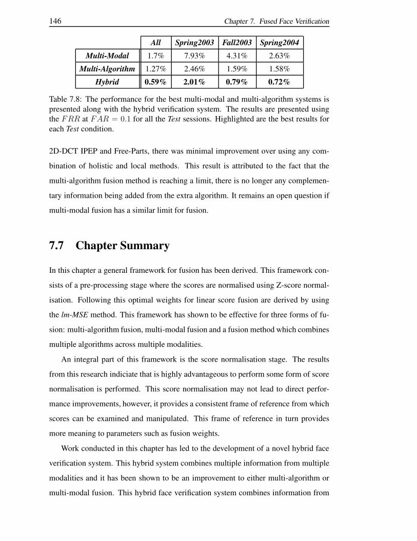
146 Chapter 7. Fused Face Verification
All Spring2003 Fall2003 Spring2004Multi-Modal 1.7% 7.93% 4.31% 2.63%
Multi-Algorithm 1.27% 2.46% 1.59% 1.58%
Hybrid 0.59% 2.01% 0.79% 0.72%
Table 7.8: The performance for the best multi-modal and multi-algorithm systems ispresented along with the hybrid verification system. The results are presented usingthe FRR at FAR = 0.1 for all the Test sessions. Highlighted are the best results foreach Test condition.
2D-DCT IPEP and Free-Parts, there was minimal improvement over using any com-
bination of holistic and local methods. This result is attributed to the fact that the
multi-algorithm fusion method is reaching a limit, there is no longer any complemen-
tary information being added from the extra algorithm. It remains an open question if
multi-modal fusion has a similar limit for fusion.
7.7 Chapter Summary
In this chapter a general framework for fusion has been derived. This framework con-
sists of a pre-processing stage where the scores are normalised using Z-score normal-
isation. Following this optimal weights for linear score fusion are derived by using
the lm-MSE method. This framework has shown to be effective for three forms of fu-
sion: multi-algorithm fusion, multi-modal fusion and a fusion method which combines
multiple algorithms across multiple modalities.
An integral part of this framework is the score normalisation stage. The results
from this research indiciate that is highly advantageous to perform some form of score
normalisation is performed. This score normalisation may not lead to direct perfor-
mance improvements, however, it provides a consistent frame of reference from which
scores can be examined and manipulated. This frame of reference in turn provides
more meaning to parameters such as fusion weights.
Work conducted in this chapter has led to the development of a novel hybrid face
verification system. This hybrid system combines multiple information from multiple
modalities and it has been shown to be an improvement to either multi-algorithm or
multi-modal fusion. This hybrid face verification system combines information from

7.7. Chapter Summary 147
the 2D and 3D face modalities using the PCA IPEP and Free-Parts algorithms. In
deriving this hybrid face verification system two important results were found.
The first result is that linear classifier fusion is robust to classifier errors. This
property is of great use as it shows that if one classifier fails the system performance
will degrade in an elegant manner, as was highlighted by the experiments for multi-
modal fusion. This result has been attributed to the fact that linear classifier score
fusion is a form of the sum rule which is robust to estimation errors.
Finally, it’s been shown that multi-modal fusion is the most consistent form of
fusion. For all the trialled multi-modal systems there was a consistent improvement in
performance. This is attributed to the fact that the data is captured by complementary
sensors; the 2D data is captured using a camera while the 3D data is captured using
a laser scanner. This improvement occurs for the fusion of the same algorithm across
two modalities as well as the fusion of multiple algorithms across the two modalities.
However, it remains to be seen if there is a limit to the complementary information
available from several modalities (more than two modalities).

148 Chapter 7. Fused Face Verification

Chapter 8
Conclusions
8.1 Introduction
This thesis has examined two issues for improving face verification:
1. The application of feature distribution modelling to:
(a) holistic features of the 2D and 3D face modalities, and
(b) Free-Parts of the 3D face modality.
2. The development of a hybrid face verification systems using:
(a) multi-algorithm fusion, and
(b) multi-modal fusion.
Feature distribution modelling for both holistic and local (Free-Parts) features is con-
sidered to provide a more complete description of the features than distance- or
angular-based similarity measures. While hybrid face verification combines comple-
mentary representations of the face, holistic and local (Free-Parts) features, using both
2D and 3D face data.
The research in the above areas has led to three main contributions, these being:
1. improving face verification by employing holistic feature distribution modelling,
2. improving 3D face verification by describing the distribution of the parts of the
3D face, and
149

150 Chapter 8. Conclusions
3. improving face verification by combining multiple algorithms across multiple
modalities.
In the following section a summary of these three contributions is provided.
8.2 Summary of Contribution
The three original contributions made in this thesis are:
(i) Improved face verification by employing holistic feature distribution
modelling
A novel method for holistic feature distribution modelling has been presented.
In order to perform holistic feature distribution modelling extra observations
of the data had to be formed. The approach taken in this thesis is to obtain
these extra observations by forming the permutations of difference vectors.
These difference vectors are then used to describe two forms of variation
Intra-Personal (IP) and Extra-Personal (EP).
The two classes of difference vectors, IP and EP, are both modelled using
GMMs. These models are then combined using a weighted LLR,
g(x) = ln(p(x | ΩIP )) − αln(p(x | ΩEP )),
so that a relevance factor α can be introduced. This relevance factor was consid-
ered necessary as the two models ΩIP and ΩEP are derived independently. The
experimental results supported the inclusion of the relevance factor as it led to
an improved verification system.
This technique for holistic feature distribution modelling, referred to as IPEP, has
been applied to both PCA and 2D-DCT features. By examining the effectiveness
of the IPEP method on two different feature vectors it has been shown that it is
a general method for holistic feature distribution modelling.
The experiments conducted for both the PCA IPEP and 2D-DCT IPEP verifi-
cation systems have shown that this method can form an improved verification

8.2. Summary of Contribution 151
system. The IPEP method was used to derive an an improved verification system
for the 3D modality and an effective verification system for the 2D modality.
(ii) Improved 3D face verification by modelling the distribution of Free-Parts
A novel technique for 3D face verification has been proposed, referred to as
the 3D Free-Parts approach. The 3D Free-Parts approach divides the face into
blocks and the distribution of these blocks are modelled. In order to model
the distribution of these blocks each block needs to be considered as a separate
observation. This is achieved by discarding the spatial relationship between each
block, forming a set of free parts.
The Free-Parts of the 3D face are represented using a frequency-based represen-
tation which is obtained using the 2D-DCT. The 2D-DCT was chosen for three
reasons, it: is computationally efficient, requires no training and ensures that
each coefficient (dimension) is orthogonal. Analysis found that the DC value,
or 0th coefficient, of the 2D-DCT had to be discarded, this is because it repre-
sents the average depth of the block and so if it was retained it would contradict
one of the assumptions of the Free-Parts approach; which is that the spatial re-
lationship between each block is discarded. This conclusion was also supported
through experimentation which showed that discarding the DC value improved
performance.
The final 3D Free-Parts verification system was found to provide a consistently
improved verification system. This verification system used GMMs to model the
Free-Parts with each client model Ωclient being formed through adaptation from
a world model Ωworld.
(iii) Improved face verification by employing hybrid methods
A novel hybrid verification system has been proposed which combines multiple
algorithms across multiple modalities. Experiments have shown that this method
for fusion outperforms either multi-algorithm or multi-modal fusion. Exper-
imentation has also highlighted that multi-modal fusion provides a consistent
improvement.
The research conducted in this thesis has found that the 2D and 3D face data

152 Chapter 8. Conclusions
(multi-modal face data) provides a consistent source of complementary infor-
mation. It was found through experimentation that fusion across the 2D and 3D
modalities led to a consistent improvement in performance; for both multi-modal
fusion and hybrid fusion. It is considered that this complementary information is
obtained because complementary sensors are used; the 2D data is captured using
a camera while the 3D data is captured using a laser scanner.
In deriving the multi-algorithm, multi-modal and hybrid fusion methods a gen-
eral framework for fusion has been proposed. This framework uses linear classi-
fier score fusion to combine information from several sources. The scores from
each classifiers are normalised to have the same range of magnitude by applying
Z-score normalisation. Following this optimal weights for linear score fusion are
derived by using the lm-MSE method. This framework has shown to be effective
for three forms of fusion: multi-algorithm fusion, multi-modal fusion and hybrid
fusion.
8.3 Future Research
This thesis has contributed to several aspects of hybrid face verification, however, there
are still several several areas that future work could address. These areas of future work
include improving the proposed methods as well as potential new research directions,
and are listed below:
• Further investigation into IPEP feature distribution modelling includes exam-
ining other holistic feature extraction techniques. Of interest is whether LDA
feature vectors, which are optimised for discrimination, will be a more suitable
feature vector.
• The 3D Free-Parts approach discards the spatial relationship between blocks.
However, the spatial relationship between features such as the eyes and nose are
considered important for human based face verification. Further investigation
could therefore investigate methods for restricting the Free-Parts approach so
that some of this spatial relationship is retained.

8.3. Future Research 153
• This research has examined the fusion of the 2D and 3D face modalities. The
fusion of these two modalities has thus far provided a consistent performance
improvement. It is therefore proposed that other face modalities such as infra-
red could be included to further improve performance and robustness.

154 Chapter 8. Conclusions

Appendix A
Mathematical Definitions
A.1 PCA Similarity Measures
Several similarity measures have been used with PCA feature vectors. The first mea-
sure proposed was the Euclidian Distance in 1991 [98]. Since then several researchers
have investigated other similarity measures, predominantly distance- or angular-based
measures.
In this Appendix a summary of the common similarity measures is provided below:
• L1 Measure (Manhattan Distance)
d(x, y) = |x − y|, (A.1)
• L2 Measure (Euclidian Distance)
d(x, y) = ‖x − y‖, (A.2)
• Cosine Measure
d(x, y) =x.y
|x||y| , (A.3)
155

156 Appendix A. Mathematical Definitions
• Mahalanobis L2 Measure
d(x, y, C) =
√
(x − y)T C−1(x − y), and (A.4)
• Mahalanobis Cosine Measure
d(u, v) =u.v
|u||v| . (A.5)
Note that x and y are the two vectors to compare, C is the diagonalised eigenvalues
found through PCA and u and v are the eigenvalue normalised vectors;
u =
[
x1√λ1
,x2√λ2
, ...,xi√λi
]
and (A.6)
v =
[
y1√λ1
,y2√λ2
, ...,yi√λi
]
. (A.7)
The Mahalanobis Cosine measure has been shown to provide optimal verification
performance [18]. This is an angular measure that uses the covariance matrix C derived
from the eigenvalues from PCA training, this measure is also known as the MahCosine
measure.

A.2. 2D DCT and Delta Coefficients 157
A.2 2D DCT and Delta Coefficients
The two-dimensions discrete cosine transform (2D-DCT) is a transform that converts
a block of values into orthogonal frequency coefficients. These coefficients have been
used for image compression in the JPEG2000 standard. The 2D-DCT converts an
image I(x, y) of size N × M to a set of coefficients,
F (u, v) =
√
2
N
√
2
M
N−1∑
x=0
M−1∑
y=0
Λ(x)Λ(y)β(u, v, x, y)I(x, y), (A.8)
where
β(u, v, x, y) = cos[π.u
2N(2x + 1)
]
cos[ π.v
2M(2y + 1)
]
(A.9)
and
Λ(ε) =
1√
2for ε = 0
1 otherwise
. (A.10)
In work conducted by Sanderson et al. [90] a modified version of the 2D-DCT was
proposed termed the DCTmod2. The DCTmod2 consists of delta coefficients where
the horizontal delta coefficient is
∆hc(b,a)n =
∑Kk=−K khkc
(b,a+k)n
∑K
k=−K hkk2(A.11)
and the vertical delta coefficient is
∆vc(b,a)n =
∑Kk=−K khkc
(b+k,a)n
∑Kk=−K hkk2
. (A.12)
Note that c(a,b)n is the nth 2D-DCT coefficient, as defined by the JPEG zig-zag pattern,
and h is a symmetric window vector of dimension 2K+1. Typically, all the values of
h are one to provide an equal weight for all the 2D-DCT coefficients. The term (b, a)
refers to the location of the block for which the coefficients are derived.

158 Appendix A. Mathematical Definitions
A.3 Fusion Methods
Several methods have been proposed for fusion. Of particular interest has been classi-
fier fusion. There are two broad aspects of classifier fusion; score fusion and decision
fusion. As the name suggests, score fusion combines scores while decision fusion com-
bines the decisions from separate classifiers. These decisions are usually represented
as yes/no answers or, more commonly, as Rank scores. The rank scores represent the
best matching ID for the ID; where Rank 1 is the best match, Rank 2 is the second best
match and Rank N is the Nth best match. In the next two sections some of the methods
to perform score and decision fusion are listed.
A.3.1 Score Fusion
Score fusion combines the scores from two or more classifiers, some of the methods to
perform this fusion are:
• sum rule
Csum =
N∑
i=1
αiCi (A.13)
• product rule
Cprod =
N∏
i=1
Cαi
i (A.14)
• min rule
Cmin(x) =N
mini=1
Ci(x) (A.15)
• max rule
Cmax(x) =N
maxi=1
Ci(x) (A.16)
• median rule
Cmedian(x) =N
mediani=1
Ci(x) (A.17)

A.3. Fusion Methods 159
where Ci is the ith classifier score and αi is the weighted for the ith classifier.
A.3.2 Decision Fusion
Decision fusion combines the decisions from two or more classifiers, two common
methods for performing decision fusion are:
• OR rule
COR =N⋂
i=1
Ci (A.18)
• AND rule
CAND =
N⋃
i=1
Ci (A.19)
where Ci is the ith classifier decision, a one or zero (binary).

160 Appendix A. Mathematical Definitions
A.4 Properties of Random Variables
There are several useful properties of random variables. The properties of interest re-
late specifically to the mean and variance of random variables. When two random
variables are added (or subtracted) or multiplied. The sample mean of a random vari-
able X is,
E(X) = x =1
N
N∑
i=1
xi, (A.20)
and the sample (and so biased) variance is,
s2N =
1
N
N∑
i=1
(xi − x)2. (A.21)
Where xi is the ith observation of X and N is the number of observations of X .
With regards to the mean, when random variables are added the mean of the resul-
tant variable Z is,
E(Z) = E(X1 + X2 + ... + Xn) = E(X1) + E(X2) + .... + E(XN), (A.22)
where n is the number of random variables added. When random variables are multi-
plied together the resultant variable Z will have a mean of,
E(Z) = E(X1X2...Xn) = E(X1)E(X2)....E(XN ), (A.23)
provided they are independent.
When performing the sum (or difference) of two zero mean random variables, X
and Y , the variance of the resultant variable Z becomes,
σ2X+Y = σ2
X + σ2Y + 2Cov(X, Y ), (A.24)
σ2X−Y = σ2
X + σ2Y + 2Cov(X, Y ). (A.25)
If the two random variables are independent we have,
σ2Z = σ2
X+Y = σ2X + σ2
Y . (A.26)

A.4. Properties of Random Variables 161
It’s noted that when multiplying a random variable by a factor of b the variance is
altered such that,
σ2bX = b2σ2
X . (A.27)

162 Appendix A. Mathematical Definitions

Bibliography
[1] FaceIt Identification SDK, Version 5.0. Identix Incorporated, NJ, USA, 2003.
[2] T. Acharya and P.-S. Tsai. JPEG2000 Standard for Image Compression: concepts,
algorithms and VLSI architectures. John Wiley & Sons, Inc., 2005.
[3] B. Achermann, X. Jiang, and H. Bunke. Face recognition using range images. Interna-
tional Conference on Virtual Systems and MultiMedia, pages 129–136, 1997.
[4] E. Alpaydin. Techniques for combining multiple learners. Proceedings of Engineering
in Intelligent Systems, 2:6–12, 1998.
[5] E. Bailly-Bailliere, S. Bengio, F. Bimbo, M. Hamouz, J. Kittler, J. Mariethoz, J. Matas,
K. Messer, V. Popovici, F. Poree, B. Ruiz, and J.-P. Thiran. The banca database and
evaluation protocol. Lecture Notes in Computer Science, pages 625–638, 2003.
[6] S. Bakshi and Y.-H. Yang. Shape from shading for non-lambertian surfaces. Proceed-
ings of the IEEE International Conference on Image Processing, 2:130 –134, 1994.
[7] M. Bartlett, J. Movellan, and T. Sejnowski. Face recognition by independent component
analysis. IEEE Transactions on Neural Networks, pages 1450–1464, 2002.
[8] P. N. Belhumeur, J. P. Hespanha, and D. J. Kriegman. Eigenfaces vs. fisherfaces: Recog-
nition using class specific linear projection. IEEE Transactions on Pattern Analysis and
Machine Intelligence, 19(7):711–720, 1997.
[9] C. BenAbdelkader and P. Griffin. Comparing and combining depth and texture cues for
face recongition. Image and Vision Computing, pages 339–352, 2004.
[10] J. Benediktsson, J. Sveinsson, and P. Swain. Hybrid consensus theoretic classification.
IEEE Transactions on Geoscience and Remote Sensing, 35:833–843, 1997.
[11] J. Benediktsson and P. Swain. Consensus theoretic classification methods. IEEE Trans-
actions on Systems Man and Cybernetics SMC, 22:668, 1992.
[12] C. Beumier and M. Acheroy. Face verification from 3d and grey level cues. Pattern
Recognition Letters, 22:1321–1329, 2001.
163

164 Bibliography
[13] R. Beveridge, D. Bolme, M. Teixeira, and B. Draper. The csu face identification eval-
uation system user’s guide: Version 5.0. http://www.cs.colostate.edu/
evalfacerec/index.html, 2003.
[14] M. Blackburn, M. Bone, and J. Phillips. Facial recognition vendor test 2000: Evaluation
report. Technical Report http://www.frvt.org/FRVT2000, 2001.
[15] V. Blanz and T. Vetter. Face recognition based on fitting a 3d morphable model. IEEE
Transactions on Pattern Analysis and Machine Intelligence, pages 1063–1074, 2003.
[16] W. W. Bledsoe. Man-machine facial recognition. Technical report for Panoramic Re-
search Inc., 1966.
[17] W. W. Bledsoe. The model method in facial recognition. Technical report for Panoramic
Research Inc., 1966.
[18] D. Bolme, J. Beveridge, M. Teixeira, and B. Draper. The csu face identification eval-
uation system: Its purpose, features, and structure. In International Conference on
Computer Vision Systems, pages 304–313, 2003.
[19] O. Bousquet and F. Perez-Cruz. Kernel methods and their applications to signal pro-
cessing. Proceedings of the IEEE International Conference on Acoustics, Speech, and
Signal Processing, pages 860–863, 2003.
[20] K. Bowyer, K. Chang, and P. Flynn. A survey of approaches to three-dimensional face
recognition. Proceedings of the 17th International Conference on Pattern Recognition,
1:358–361, 2004.
[21] A. M. Bronstein, M. M. Bronstein, and R. Kimmel. Expression-invariant 3d face recog-
nition. Audio- and Video-Based Person Authentication, pages 62–70, 2003.
[22] N. Brummer. Tools for fusion and calibration of automatic speaker detection systems.
http://www.dsp.sun.ac.za/˜nbrummer/focal/index.htm, 2005.
[23] J. Y. Cartoux, J. T. Lapreste, and M. Richetin. Face authentication or recognition by
profile extraction from range images. Workshop on Interpretation of 3D Scenes, pages
194–199, 1989.
[24] K. I. Chang, K. W. Bowyer, and P. J. Flynn. Face recognition using 2d and 3d facial
data. Workshop in Multimodal User Authentication, pages 25–32, 2003.
[25] R. Chellappa, C. L. Wilson, and S. Sirohey. Human and machine recognition of faces:
A survey. Proceedings of the IEEE, 83:705 –741, 1995.
[26] L. Chen, H. Liao, M. Ko, J. Lin, and G. Yu. A new lda-based face recognition system
which can solve the small sample size problem. Pattern Recognition, pages 1713–1726,
2000.

Bibliography 165
[27] J. Cook, V. Chandran, S. Sridharan, and C. Fookes. Face recognition from 3d data
using iterative closest point algorithm and gaussian mixture models. Proceedings of the
2nd International Symposium on 3D Data Processing, Visualization and Transmission,
pages 502–509, 2004.
[28] J. Cook, V. Chandran, S. Sridharan, and C. Fookes. Gabor filter bank representation
for 3d face recognition. Proceedings of Digital Image Computing: Techniques and
Applications, pages 16–23, 2005.
[29] J. Cook, C. McCool, V. Chandran, and S. Sridharan. Combined 2d/3d face recongition
using log-gabor templates. AVSS, 2006.
[30] G. R. Cooper and C. D. McGillem. Probabilistic methods of signal and system analysis.
Oxford University Press, 1999.
[31] Cyberware. Cyberware model 3030 head scanner. http://www.cyberware.
com/products/scanners/3030.html, 2006.
[32] J. Daugman. Biometric decision landscapes. Technical Report TR482 for University of
Cambridge, 2000.
[33] K. Delac, M. Grgic, and S. Grgic. Statistics in face recognition: Analyzing probability
distributions of pca, ica and lda performance results. Proceedings of the 4th Interna-
tional Symposium on Image and Signal Processing and Analysis, pages 289–294, 2004.
[34] U. R. Dhond and J. K. Aggarwal. Structure from stereo - A review. IEEE Trans. Syst.,
Man, Cybern., 19(6):1489–1510, 1989.
[35] G. Doddington, M. Przybocki, A. Martin, and D. Reynolds. The NIST speaker recogni-
tion evaluation — overview, methodology, systems, results, perspective. Speech Com-
munication, 31(2-3):225–254, 2000.
[36] B. Duc, S. Fischer, and J. Bigun. Face authentication with gabor information on de-
formable graphs. IEEE Trans. on Image Processing, pages 504–516, 1999.
[37] R. O. Duda, P. E. Hart, and D. G. Stork. Pattern Classification: 2nd Edition. John
Wiley and Sons, Inc., 2001.
[38] M. I. Fanany, M. Ohno, and I. Kumazawa. A scheme for reconstructing face from shad-
ing using smooth projected polygon representation nn. Proceeding of the International
Conference on Image Processing, 2:305–308, 2002.
[39] F. Forster, P. Rummel, M. Lang, and B. Radig. The hiscore camera a real time three
dimensional and color camera. International Conference on Image Processing, pages
598–601, 2001.

166 Bibliography
[40] K. Fukunaga. Introduction to Statistical Pattern Recognition. Academic Press, New
York, 1990.
[41] G. G. Gordon. Face recognition based on depth maps and surface curvature. in SPIE
Proceedings, 1570:234–247, 1991.
[42] F. Goudail, E. Lange, T. Iwamoto, K. Kyuma, and N. Otsu. Face recognition system
using local autocorrelations and multiscale integration. IEEE Trans on Pattern Analysis
Matching and Intelligence, pages 1024–1028, 1996.
[43] R. Gross and V. Brajovic. An image preprocessing algorithm for illumination invariant
face recognition. Lecture Notes in Computer Science, pages 10–18, 2003.
[44] M. Grudin. On internal representations in face recognition systems. Pattern Recogni-
tion, pages 1161–1177, 2000.
[45] P. L. Hallinan, G. G. Gordon, A. L. Yuille, P. Giblin, and D. Mumford. Two- and
Three-Dimensional Patterns of Face. A K Peters, Ltd., 1999.
[46] L. Harmon and W. Hunt. Automatic recognition of human face profiles. Computer
Graphics and Image Process., pages 135–156, 1977.
[47] A. Jain, K. Nandakumar, U. Uludag, and X. Lu. Multimodal Biometrics: Augmenting
Face With Other Cues, pages 679–705. Elsevier Inc., 2006.
[48] Z. Jiali, W. Jinwei, and L. Siwei. Face recognition: a facial action reconstruction and
ica representation approach. Proceedings of the 2001 International Conferences on
Info-tech and Info-net, 3:456–461, 2001.
[49] T. Kanade. Picture processing by computer complex and recognition of human faces.
Technical Report: Kyoto University, Dept. of Information Science, 1973.
[50] J. Kittler, M. Hatef, R. P. W. Duin, and J. Matas. On combining classifiers. IEEE
Transactions on Pattern Analysis and Machine Intelligence, 20:226–239, 1998.
[51] M. Lades, J. Vorbruggen, J. Buhmann, J. Lange, and C. Malsburg. Distortion invariant
object recognition in the dynamic link architecture. IEEE Trans. Computers, pages
300–311, 1993.
[52] C. Lee and J. Gauvain. Bayesian adaptive learning and MAP estimation of HMM, pages
83–107. Kluwer Academic Publishers, Boston, Massachusetts, USA, 1996.
[53] J. C. Lee and E. Milios. Matching range images of human faces. Proc. IEEE ICCV,
pages 722–726, 1990.
[54] R. Lengagne, R. Fua, and O. Monga. 3d face modeling from stereo and differential con-
straints. Proc. IEEE Automatic Face and Gesture Recognition, pages 148–153, 1998.

Bibliography 167
[55] R. Lengagne, J.-P. Tarel, and O. Monga. From 2d images to 3d face geometry. Proceed-
ings of the Second International Conference on Automatic Face and Gesture Recogni-
tion, pages 301–306, 1996.
[56] J. Li, S. Zhou, and C. Shekhar. A comparison of subspace analysis for face recognition.
Proceedings of the IEEE International Conference on Acoustics, Speech, and Signal
Processing, pages 121–124, 2003.
[57] S. Lowther, C. McCool, V. Chandran, and S. Sridharan. Improving face localisation us-
ing claimed identity for face recognition. Proceedings of the 3rd Interational Workshop
on the Internet, Telecommunications and Signal Processing, 2004.
[58] J. Lu, K. Plataniotis, and A. Venetsanopoulos. Regularized d-lda for face recognition.
ICASSP 2003, pages 125–128, 2003.
[59] S. Lucey. The symbiotic relationship of parts and monolithic face representations in ver-
ification. Proceedings of IEEE Conference of Computer Vision and Pattern Recognition
Workshop, page 89, 2004.
[60] S. Lucey and T. Chen. Integrating monolithic and free-parts representations for im-
proved face verification in the presence of pose mismatch. Technical Report for CMU,
2004.
[61] S. Lucey and T. Chen. Improved face recognition through mismatch driven represen-
tations of the face. International Conference on Computer Vision (ICCV) Workshop,
2006.
[62] S. Lucey and C. Sanderson. Synthesized gmm free-parts based face representation for
pose mismatch reduction in face verification. Technical Report for CMU, 2004.
[63] A. Martin, G. Doddington, T. Kamm, M. Ordowski, and M. Przybocki. The DET curve
in assessment of detection task performance. In Eurospeech, volume 4, pages 1895–
1898, 1997.
[64] A. Martin and M. Przybocki. The nist 1999 speaker recognition evaluation—an
overview. Digital Signal Processing, 10(1-3):1–18, 2000.
[65] C. McCool, V. Chandran, and S. Sridharan. 2d-3d hybrid face recognition based on
pca and feature modelling. Proceedings of the 2nd Workshop on Multimodal User
Authentication, 2006.
[66] K. Messer, J. Kittler, M. Sadeghi, M. Hamouz, A. Kostin, F. Cardinaux, S. Marcel,
S. Bengio, C. Sanderson, N. Poh, Y. Rodriguez, J. Czyz, L. Vandendorpe, C. Mc-
Cool, S. Lowther, S. Sridharan, V. Chandran, R. P. Palacios, E. Vidal, L. Bai, L. Shen,

168 Bibliography
Y. Wang, C. Yueh-Hsuan, L. Hsien-Chang, H. Yi-Ping, A. Heinrichs, M. Muller,
A. Tewes, C. von der Malsburg, R. Wurtz, Z. Wang, F. Xue, Y. Ma, Q. Yang, C. Fang,
X. Ding, S. Lucey, R. Goss, and H. Schneiderman. Face authentication test on the
banca database. ICPR 2004. Proceedings of the 17th International Conference on Pat-
tern Recognition, 4:523–532, 2004.
[67] K. Messer, J. Kittler, M. Sadeghi, M. Hamouz, A. Kostin, S. Marcel, S. Bengio, F. Car-
dinaux, C. Sanderson, N. Poh, Y. Rodriguez, K. Kryszczuk, J. Czyz, L. Vandendorpe,
J. Ng, H. Cheung, and B. Tan. Face authentication competition on the banca database.
Proceedings of the Internation Conference on Biometric Authentication 2004, pages
8–15, 2004.
[68] K. Messer, J. Matas, J. Kittler, J. Leuttin, and G. Maitre. Xm2vtsdb: The extended
m2vts database. Second International Conference on Audio and Vdeo-base Biometric
Person Authentication, 1999.
[69] Minolta. Konica minolta vivid 910 website. http://se.konicaminolta.us/
products/3d_scanners/vivid_910/index.html, 2006.
[70] B. Moghaddam, T. Jebara, and A. Pentland. Bayesian face recognition. Pattern Recog-
nition, 23:1771–1782, 2000.
[71] B. Moghaddam and A. Pentland. Beyond euclidean eigenspaces: Bayesian matching
for visual recognition, 1998.
[72] H. Moon and P. J. Phillips. Analysis of pca-based face recognition algorithms. Em-
pirical Evluation Techniques in Computer Vision, Editors: K. Bowyer and P. Phillips,
pages 57–71, 1998.
[73] H. Moon and P. J. Phillips. Computational and performance aspects of pca-based face-
recognition algorithms. Perception, pages 303–321, 2001.
[74] T. Nagamine, T. Uemura, and I. Masuda. 3d facial image analysis for human identifi-
cation. International Conference on Pattern Recognition, page 324, 1992.
[75] K. Najim, E. Ikonen, and A. Daoud. Stochastic processes: estimation, optimization and
analysis. Kogan Page Science, London and Sterling, VA, 2004.
[76] A. Nefian and M. H. H. III. Hidden markov models for face recognition. Proceedings of
the 1998 IEEE International Conference on Acoustics, Speech, and Signal Processing,
5:2721–2724, 1998.
[77] A. Nefian and M. H. H. III. An embdedded hmm-based approach for face detection
and recognition. Proceedings of the 1999 IEEE International Conference on Acoustics,
Speech, and Signal Processing, 6:3553–3556, 1999.

Bibliography 169
[78] Z. Pan, A. G. Rust, and H. Bolouri. Image redundancy reduction for neural network
classification using discrete cosine transforms. International Joint Conference on Neu-
ral Networks 2000, 3:149–154, 2000.
[79] P. Penev and J. Atick. Local feature analysis: a general statistical theory for object
representation. Computation in Neural Systems, pages 477–500, 1996.
[80] J. Phillips, P. Flynn, T. Scruggs, K. Bowyer, J. Chang, K. Hoffman, J. Marques, J. Min,
and W. Worek. Overview of the face recognition grand challenge. Proceedings of IEEE
Conference of Computer Vision and Pattern Recognition, 1:947–954, 2005.
[81] J. Phillips, P. Grother, R. J. Micheals, D. Blackburn, E. Tabassi, and M. Bone. Face
recognition vendor test 2002: Overview and summary. IEEE Workshop on Analysis
and Modeling of Faces and Gestures, page 44, 2003.
[82] K. R. Rao and P. Yip. Discrete Cosine Transform. Academic Press, 1990.
[83] D. Reynolds. Comparison of background normalization methods for text-independent
speaker verification. Proc. European Conference on Speech Communication and Tech-
nology (Eurospeech), 2:963–966, 1997.
[84] D. A. Reynolds. A gaussian mixture modeling approach to text-independent speaker
identification. Ph.D. thesis, Georgia Institute of Technology, 1992.
[85] D. A. Reynolds, T. F. Quatieri, and R. B. Dunn. Speaker verification using adapted
gaussian mixture models. Digital Signal Processing, 10:19–41, 2000.
[86] S. Sakamoto, I. J. Cox, and J. Tajima. A multiple-baseline stereo for precise human
face acquisition. Pattern Recognition Letters, 18:923–931, 1997.
[87] F. Samaria and F. Fallside. Face identification and feature extraction using hidden
markov models. Image Processing: Theory and Applications, pages 295–298, 1993.
[88] F. Samaria and S. Young. Hmm-based architecture for face identification. Image and
Vision Computing, 12(8):537–543, 1994.
[89] C. Sanderson. Face processing & frontal face verification. IDIAP Research Report,
2003.
[90] C. Sanderson and K. K. Paliwal. Fast feature extraction method for robust face verifi-
cation. Electronic Letters, 38(25):1648–1650, 2002.
[91] C. Sanderson, M. Saban, and Y. Gao. A study of loca features for unconstrained parts
based face classification. Technical Report for NICTA, 2006.
[92] M. Savvides and B. V. Kumar. Efficient design of advanced correlation filters for robust
distortion-tolerant face recognition. Proceedings of the IEEE Conference on Advanced
Video and Signal Based Surveillance, 2003.

170 Bibliography
[93] M. Savvides, B. V. Kumar, and P. Khosla. Face verification using correlation filters.
Proceedings of third IEEE Automatic Identification Advanced Technologies, pages 56–
61, 2002.
[94] D. Scharstein and R. Szeliski. A taxonomy and evaluation of dense two-frame stereo
correspondence algorithms. Microsoft Research Technical Report MSR-TR-2001-8,
2001.
[95] D. Sheskin. Handbook of Parametric and Nonparametric Statistical Procedures, pages
181–188. Chapman and Hall/CRC, 2004.
[96] L. Sirovich and M. Kirby. Low-dimensional procedure for the characterization of hu-
man faces. Journal of Optical Society of America, pages 519–524, 1987.
[97] F. Tsalakanidou, D. Tzovaras, and M. G. Strintzis. Use of depth and colour eigenfaces
for face recognition. Pattern Recognition Letters, 24:427–435, 2003.
[98] M. Turk and A. Pentland. Eigenfaces for recognition. Journal of Cognitive Neuro-
science, 3(1):71–86, 1991.
[99] R. Vogt, J. Pelecanos, and S.Sridharan. Dependence of gmm adaptation on feature
post-processing. Eurospeech, pages 3013–3016, 2003.
[100] F. Wallhoff, S. Eickeler, and G. Rigoll. A comparison of discrete and continuous output
modelling techniques for a pseudo-2d hidden markov model face recognition system.
International Conference on Image Processing, 2:685–688, 2001.
[101] Y. Wang, C. Chua, and Y. Ho. Face recognition from 2d and 3d images using structural
hausdorff distance. Proceedings of the Seventh International Conference on Control,
Automation, Robotics and Vision, pages 502–507, 2002.
[102] Y. Wang, C. Chua, and Y. Ho. Facial feature detection and face recognition from 2d and
3d images. Pattern Recognition Letters, 23:1191–1202, 2002.
[103] Y. Wang, C. Chua, Y. Ho, and Y. Ren. Integrated 2d and 3d images for face recognition.
Proceedings of the 11th International Conference on Image Analysis and Processing,
pages 48–53, 2002.
[104] L. Wiskott, J. Fellous, N. Kruger, and C. von der Malsburg. Face recognition by elastic
bunch graph matching. IEEE Transactions on Pattern Analysis and Machine Intelli-
gence, 19(7):775–779, 1997.
[105] L. Wiskott, J. Fellous, N. Kruger, and C. von der Malsburg. Face recognition by elastic
bunch graphing. In Intelligent Biometric Techniques in Fingerprint and Face Recogni-
tion, pages 355–396, 1999.

Bibliography 171
[106] T. T. Y. Fang and Y. WAng. Fusion of global and loca features for face verification.
Internation Conference on Pattern Recognition, pages 382–385, 2002.
[107] W. S. Yambor, B. A. Draper, and J. R. Beveridge. Analyzing pca-based face recognition
algorithms: Eigenvector selection and distance measures. 2nd Workshop on Empirical
Evaluation in Computer Vision, 2000.
[108] J. Yang, D. Zhang, and J. Yang. Is ica significantly better than pca for face recognition?
Proceedings of the Tenth IEEE International Conference on Computer Vision, 1:198–
203, 2005.
[109] M.-H. Yang, N. Ahuja, and D. Kriegman. Face recognition using kernel eigenfaces.
Proceedings of the International Conference on Image Processing, 1:37–40, 2000. 0-
7803-6297-7/00.
[110] H. Yu and J. Yang. A direct lda algorithm for high-dimensional data - with application
to face recognition. Pattern Recognition Letters, 2001.
[111] W. Zhao, R. Chellappa, P. Phillips, and A. Rosenfeld. Face recognition: A literature
survey. ACM Computing Surveys, 35(4):399–459, 2003.