abstract dissertation: deep adversarial approaches in

ABSTRACT

Title of Dissertation: DEEP ADVERSARIAL APPROACHES IN

RELIABILITY David Benjamin Verstraete, Doctor of

Philosophy, 2019 Dissertation directed by: Professor Mohammad Modarres, Department of

Mechanical Engineering, Center of Risk and Reliability Associate Professor Enrique Lopez Droguett, Department of Mechanical Engineering, Center of Risk and Reliability

Reliability engineering has long been proposed with the problem of predicting failures

using all available data. As modeling techniques have become more sophisticated, so

too have the data sources from which reliability engineers can draw conclusions. The

Internet of Things (IoT) and cheap sensing technologies have ushered in a new

expansive set of multi-dimensional big machinery data in which previous reliability

engineering modeling techniques remain ill-equipped to handle. Therefore, the

objective of this dissertation is to develop and advance reliability engineering research

by proposing four comprehensive deep learning methodologies to handle these big

machinery data sets. In this dissertation, a supervised fault diagnostic deep learning

approach with applications to the rolling element bearings incorporating a deep

convolutional neural network on time-frequency images was developed. A semi-

supervised generative adversarial networks-based approach to fault diagnostics using

the same time-frequency images was proposed. The time-frequency images were used

again in the development of an unsupervised generative adversarial network-based

methodology for fault diagnostics. Finally, to advance the studies of remaining useful

life prediction, a mathematical formulation and subsequent methodology to combine

variational autoencoders and generative adversarial networks within a state-space

modeling framework to achieve both unsupervised and semi-supervised remaining

useful life estimation was proposed.

All four proposed contributions showed state of the art results for both fault diagnostics

and remaining useful life estimation. While this research utilized publicly available

rolling element bearings and turbofan engine data sets, this research is intended to be a

comprehensive approach such that it can be applied to a data set of the engineer’s

chosen field. This research highlights the potential for deep learning-based approaches

within reliability engineering problems.

DEEP ADVERSARIAL APPROACHES IN RELIABILITY

by

David Benjamin Verstraete

Dissertation submitted to the Faculty of the Graduate School of the University of Maryland, College Park, in partial fulfillment

of the requirements for the degree of Doctor of Philosophy

2019 Advisory Committee: Professor Mohammad Modarres, Chair Associate Professor Enrique Lopez Droguett Assistant Professor Mark Fuge Assistant Professor Katrina Groth Professor Balakumar Balachandran Professor Mohamad Al-Sheikhly (Dean’s Representative)

© Copyright by David Benjamin Verstraete

2019

ii

Dedication

To Lisa, for your love and patience.

To Will and Veronica, for your understanding and willingness to let dad sit at his

desk for hours on the weekends.

To my parents, thank you for your support, countless meals, and free babysitting.

iii

Acknowledgements

I would be remised without acknowledging the incredible help Dr. Droguett and Dr.

Modarres have been throughout this process. Your patience and willingness to advise

a distance student in Michigan was instrumental to the success of this research. I could

not have completed this research with different advisors.

I would like to thank my dissertation committee members Dr. Mark Fuge, Dr. Katrina

Groth, Dr. Balakumar Balachandran, Dr. Mohamad Al-Sheikhly, and Dr. Gregory B.

Baecher. Your valuable help and feedback on my dissertation improved this research.

iv

Table of Contents Dedication ..................................................................................................................... ii

Acknowledgements ...................................................................................................... iii Table of Contents ......................................................................................................... iv List of Tables .............................................................................................................. vii

List of Figures .............................................................................................................. ix List of Abbreviations ................................................................................................... xi Chapter 1: Introduction ................................................................................................. 1

1.1 Motivation and Background ............................................................................... 1 1.2 Research Objective ............................................................................................. 2 1.3 Methodology ....................................................................................................... 3

1.3.1 Investigate the Application of Deep Learning Algorithms .......................... 4

1.3.2 Deep Learning Enabled Supervised Fault Diagnostics ................................ 4

1.3.3 Unsupervised Fault Diagnostics .................................................................. 5

1.3.3 Semi-Supervised Fault Diagnostics ............................................................. 5

1.3.4 Advance the Studies of Unsupervised Remaining Useful Life Prognostics. 6 1.3.5 Advance the Studies of Semi-Supervised Remaining Useful Life Prognostics ............................................................................................................ 7

Chapter 2: Deep Learning Enabled Fault Diagnosis Using Time-Frequency Image Analysis of Rolling Element Bearings .......................................................................... 8

2.1 Abstract ............................................................................................................... 8 2.2 Introduction ......................................................................................................... 8 2.3 Deep Learning and CNN Background .............................................................. 14

2.4 Time Frequency Methods Definition and Discussion ...................................... 18

2.4.1 Spectrograms – Short-Time Fourier Transform (STFT) ........................... 19

2.4.2 Scalograms – Wavelet Transform .............................................................. 20

2.4.3 Hilbert-Huang Transform (HHT) .............................................................. 22

2.5 Proposed CNN Architecture for Fault Classification Based on Vibration Signals ..................................................................................................................... 24 2.6 Case Study 1: Machinery Failure Prevention Technology (MFPT) ................. 27

2.7 Case Study 2: Case Western Reserve (CWR) University Bearing Data Center 35

2.8 Scalograms with Noise ..................................................................................... 43 2.9 Traditional Feature Extraction .......................................................................... 45

2.9.1 Description of Features .............................................................................. 45 2.9.2 Application to CNN Architecture .............................................................. 46

2.10 Concluding Remarks ....................................................................................... 47 Chapter 3: Unsupervised Deep Generative Adversarial Based Methodology for Automatic Fault Detection .......................................................................................... 50

3.1 Abstract ............................................................................................................. 50 3.2 Introduction ....................................................................................................... 51 3.3 Generative Adversarial Networks ..................................................................... 52

3.3.1 Strided Convolutions ................................................................................. 56 3.3.2 Batch Normalization .................................................................................. 56 3.3.3 Activation Layers ....................................................................................... 57

v

3.3.4 Neural Network Architectures ................................................................... 57

3.4 Propose Methodology Application ................................................................... 58

3.5 Conclusions ....................................................................................................... 62 Chapter 4: Deep Semi-Supervised Generative Adversarial Fault Diagnostics of Rolling Element Bearings. .......................................................................................... 64

4.1 Abstract ............................................................................................................. 64 4.2 Introduction ....................................................................................................... 64 4.3 Background on Adversarial Training ................................................................ 68

4.3.1 Clustering ................................................................................................... 70 4.4 Proposed Generative Adversarial Fault Diagnostic Methodology ................... 71

4.4.1 Read Raw Signal and Image Representation Construction ....................... 79

4.4.2 Unsupervised GAN Initialization .............................................................. 79

4.4.3 Concatenation, Normalization, and Clustering .......................................... 81

4.4.4 Unsupervised Visual Evaluation – PCA .................................................... 81

4.4.5 Label Data .................................................................................................. 82 4.4.6 Semi-Supervised GAN Initialization ......................................................... 82

4.4.7 Semi-Supervised Stop Criteria ................................................................... 84

5.0 Examples of Application................................................................................... 84 5.1 Machinery Failure Prevention Technology Data Set .................................... 84

5.2 Case Western Reserve University Bearing Data Set .................................... 93

6.0 Comparison with AE and VAE....................................................................... 100

7.0 Concluding Remarks ....................................................................................... 108 8.0 Appendix A ..................................................................................................... 111 9.0 Appendix B ..................................................................................................... 113 10.0 Appendix C ................................................................................................... 114

Chapter 5: A Deep Adversarial Approach Based on Multi-Sensor Fusion for Remaining Useful Life Prognostics .......................................................................... 115

5.1 Abstract ........................................................................................................... 115 5.2 Introduction ..................................................................................................... 115 5.3 Background ..................................................................................................... 117

5.3.1 Generative Adversarial Networks ............................................................ 117

5.3.2 Variational Autoencoders ........................................................................ 118

5.4 Proposed Framework ...................................................................................... 119 5.5 Experimental Results ...................................................................................... 121 5.6 Conclusions ..................................................................................................... 123

Chapter 6: A Deep Adversarial Approach Based on Multi-Sensor Fusion for Semi-Supervised Remaining Useful Life Prognostics ....................................................... 124

6.1 Abstract ........................................................................................................... 124 6.2 Introduction ..................................................................................................... 124 6.3 Background ..................................................................................................... 127

6.3.1 Generative Adversarial Networks ............................................................ 128

6.3.2 Variational Autoencoders ........................................................................ 129

6.4 Proposed Methodology ................................................................................... 131 6.4.1 Unsupervised Remaining Useful Life Formulation ................................. 133

6.4.2 Semi-Supervised Loss Function .............................................................. 138

6.5 Experimental Results ...................................................................................... 139

vi

6.5.1 CMAPSS Results ..................................................................................... 141 6.5.2 Ablation Study Results ............................................................................ 145 6.5.3 FEMTO Bearing Results.......................................................................... 148

6.6 Conclusions ..................................................................................................... 150 Chapter 7: Conclusions, Contributions, and Future Research Recommendations .. 152

7.1 Conclusions ..................................................................................................... 152 7.2 Future Research Recommendations ................................................................ 155

Bibliography ............................................................................................................. 157

vii

List of Tables Table 2-1: Overview of CNN architectures used for fault diagnosis. ......................... 26

Table 2-2: Overview of learnable parameters for the CNN architectures. ................. 26

Table 2-3: MFPT baseline images. ............................................................................. 29 Table 2-4: MFPT inner race images. .......................................................................... 29 Table 2-5: MFPT outer race images. .......................................................................... 29 Table 2-6: Prediction accuracies for 32x32 pixel image inputs. ................................. 30

Table 2-7: Prediction accuracies for 96x96 pixel image inputs. ................................. 31

Table 2-8: MFPT paired two-tailed t-test p-values. .................................................... 32

Table 2-9: Confusion matrices for MFPT (A) 96x96 and (B) 32x32 scalograms for the proposed architecture. ........................................................................................... 33 Table 2-10: Precision for MFPT data set. ................................................................... 33 Table 2-11: Sensitivity for MFPT data set. ................................................................. 33 Table 2-12: Specificity for MFPT data set. ................................................................ 33 Table 2-13: F-Measure for MFPT data set. ................................................................ 34

Table 2-14: CWR baseline images. ............................................................................ 38 Table 2-15: CWR inner race images. .......................................................................... 38 Table 2-16: CWR ball fault images. ........................................................................... 39 Table 2-17: CWR outer race images. .......................................................................... 39 Table 2-18: Prediction accuracies for 32x32 image inputs. ........................................ 40

Table 2-19: Prediction accuracies for 96x96 image inputs. ........................................ 40

Table 2-20: CWR paired two-tailed t-test p-values. ................................................... 41

Table 2-21: Confusion matrix for CWR (A) 96x96 and (B) 32x32 scalograms for the proposed architecture .................................................................................................. 41 Table 2-22: Precision for CWR data set. .................................................................... 42 Table 2-23: Sensitivity for CWR data set. .................................................................. 42 Table 2-24: Specificity for CWR data set. .................................................................. 42 Table 2-25: F-Measure for CWR data set. .................................................................. 43 Table 2-26: MFPT 96x96 scalogram images with noise injected............................... 44

Table 2-27: Prediction accuracies for MFPT scalograms with injected noise. ........... 45

Table 2-28: Prediction accuracies for CWR. .............................................................. 46

Table 2-29: Prediction accuracies for MFPT. ............................................................. 47

Table 3-1: 96x96 pixel MFPT scalogram images. ...................................................... 59

Table 3-2: MFPT 96x96 generator output, DCGAN, Kmeans++. ............................. 62

Table 4-1: 96x96 pixel MFPT scalogram images (actual size). ................................. 86

Table 4-2: Fully unsupervised 32x32 generator output, InfoGAN LA output and spectral clustering. ...................................................................................................... 91 Table 4-3: 32x32 generator output, InfoGAN LA output and spectral clustering. ..... 92

Table 4-4: 96x96 pixel CWR scalogram images of the faults. ................................... 96

Table 4-5: CWR 96x96 generator output, DCGAN kmeans++ clustering. ................ 98

Table 4-6: CWR 96x96 generator output, DCGAN kmeans++ clustering. ................ 99

Table 4-7: MFPT Unsupervised AE and VAE results. ............................................. 102

Table 4-8: CWR Unsupervised AE and VAE results. .............................................. 107

Table 6-1: CMAPSS Data Overview ........................................................................ 140

viii

Table 6-10: FD001 RMSE Unsupervised feature learning with semi-supervised regression .................................................................................................................. 142 Table 6-11: FD001 RMSE Semi-supervised feature learning with semi-supervised regression .................................................................................................................. 143 Table 6-12: FD004 RMSE Unsupervised feature learning with semi-supervised regression .................................................................................................................. 144 Table 6-13: FD004 RMSE Semi-supervised feature learning with semi-supervised regression .................................................................................................................. 144 Table 6-14: FD001 RMSE Unsupervised Feature Learning – Fixed Labeling Intervals................................................................................................................................... 145

Table 6-15: FD001 RMSE Unsupervised Feature Learning – Random Labeling Intervals..................................................................................................................... 146 Table 6-16: Unsupervised RMSE average results for the C-MAPSS test set........... 148

Table 6-17: FEMTO Dataset Information ................................................................ 149

Table 6-18: FEMTO RMSE Results – Semi-supervised Feature Learning with Semi-Supervised regression. .............................................................................................. 150

ix

List of Figures Figure 2-1:Generic CNN architecture. ........................................................................ 15 Figure 2-2: Process of representations for time-frequency analysis. .......................... 18

Figure 2-3: STFT spectrogram of baseline raw signal. ............................................... 20

Figure 2-4: Wavelet transform scalogram of baseline raw signal. ............................. 22

Figure 2-5: Overview of HHT adapted from [4]. ....................................................... 23

Figure 2-6: HHT image of baseline raw signal. .......................................................... 24

Figure 2-7: Proposed CNN architecture. .................................................................... 25 Figure 2-8: Test stand for roller bearing accelerometer data. ..................................... 36

Figure 3-1: GAN Training .......................................................................................... 53 Figure 3-2: Proposed Unsupervised GAN Methodology............................................ 55

Figure 3-3: Generator Network ................................................................................... 58 Figure 3-4: Discriminator Network ............................................................................ 58 Figure 3-5: Output images of DCGAN generator training. ........................................ 60

Figure 3-6: DCGAN PCA KMeans ++ predicted. ...................................................... 61

Figure 3-7: DCGAN PCA Kmeans ++ real. ............................................................... 61

Figure 4-1: GAN overview. ........................................................................................ 68 Figure 4-2: Proposed generative adversarial fault diagnostic methodology. .............. 75

Figure 4-3: Generator Network ................................................................................... 76 Figure 4-4: Discriminator Network ............................................................................ 77 Figure 4-5: InfoGANs discriminator network. ........................................................... 78

Figure 4-6: Baseline signal. ........................................................................................ 85 Figure 4-7: Inner race fault signal. .............................................................................. 85 Figure 4-8: Outer race fault signal. ............................................................................. 86 Figure 4-9: Output images of DCGAN generator training model. ............................. 87

Figure 4-10: Output images of InfoGAN generator training model. .......................... 87

Figure 4-11: Spectral clustering PCA, InfoGAN LA output image 32x32 pixels. ..... 89

Figure 4-12: CWR experimental test stand for roller bearing. ................................... 94

Figure 4-13: Baseline raw signal. ............................................................................... 95 Figure 4-14: Inner race fault raw signal. ..................................................................... 95 Figure 4-15: Outer race fault raw signal. .................................................................... 95 Figure 4-16: Ball fault raw signal. .............................................................................. 95 Figure 4-17: Output images of DCGAN generator training model. ........................... 96

Figure 4-18: Output images of InfoGAN generator training model. .......................... 97

Figure 4-19: K-means++ PCA, DCGAN LA output image 96x96 pixels. ................. 97

Figure 4-20: MFPT AE MLP architecture. ............................................................... 102

Figure 4-21: MFPT AE convolutional architecture. ................................................. 103

Figure 4-22: MFPT VAE convolutional architecture. .............................................. 104

Figure 4-23: CWR AE MLP architecture. ................................................................ 105

Figure 4-24: CWR AE convolutional architecture. .................................................. 106

Figure 4-25: CWR VAE convolutional architecture. ............................................... 107

Figure 5-1: Simplified diagram of engine simulated in C-MAPPS [67]. ................. 122

Figure 5-27: FD001 RMSE results vs training step for 50 iterations with the lowest result (14.69) marked. ............................................................................................... 122 Figure 6-28: Generative and inference modeling similarities (Adapted from [91]). 128 Figure 6-29: Generative Adversarial Networks ........................................................ 129

x

Figure 6-30: Variational autoencoder ....................................................................... 130 Figure 6-31: Proposed deep generative methodology for remaining useful life estimation. ................................................................................................................. 132 Figure 6-32: Forward graphical model for the proposed mathematical framework. 134

Figure 6-33: Inference training model. ..................................................................... 134 Figure 6-34: Simplified diagram of engine simulated in C-MAPSS [67]. ............... 140

Figure 6-35: FD001 RMSE versus percent labeled (%). .......................................... 143

Figure 6-36: FD004 RMSE versus percent labeled (%). .......................................... 144

Figure 6-37: FD001 Unsupervised Feature Learning, Random Labeling Intervals . 147 Figure 6-38: FD001 Unsupervised Feature Learning, Random Labeling Intervals . 147

Figure 6-39: Overview of PRONOSTIA [97] .......................................................... 149

xi

List of Abbreviations • IoT - Internet of Things

• RUL - Remaining Useful Life

• CNN – Convolutional Neural Network

• GAN – Generative Adversarial Network

• VAE – Variational Autoencoder

• DCGAN – Deep Convolutional Generative Adversarial Network

• InfoGAN – Information Maximizing Generative Adversarial Network

• STFT - Short-Time Fourier Transform

• WT – Wavelet Transform

• HHT - Hilbert-Huang Transform

• NMI – Normalized Mutual Information

• ARI - Adjusted Rand Index

• ESREL - European Safety and Reliability

• PHM – Prognostics and Health Management

• OEM – Original Equipment Manufacturer

• MFPT - Machinery Failure Prevention Technology

• CWR – Case Western Reserve

• SVM – Support Vector Machine

of 183

Chapter 1: Introduction

1.1 Motivation and Background

Reliability engineering has long been posed with the problem of predicting failures

using all data available. As modeling techniques have become more sophisticated, so

have the data sources from which reliability engineers can draw conclusions. The IoT

and cheap sensing technologies have ushered in a new expansive set of multi-

dimensional data which previous reliability engineering modeling techniques are

unequipped to handle.

Diagnosis and prognosis of faults and RUL predictions with this new data are of great

economic value as equipment customers are demanding the ability of the assets to

diagnose faults and alert technicians when and where maintenance is needed [1]. RUL

predictions, being the most difficult, are also of the most value for the asset owner.

They provide information for a state-of-the-art maintenance plan which reduces

unscheduled maintenance costs by avoiding downtime and safety issues.

This new stream of data is often too costly and time consuming to justify labeling all

of it. Therefore, taking advantage of unsupervised learning-based methodologies

would have greatest economic benefit. Deep learning has emerged as a strong

unsupervised feature extractor without the need for previous knowledge of relevant

features on a labeled data set [2]. If faulty system states are unavailable or a small

percentage of the fault data is labeled, deep generative modeling techniques have

of 183

shown the ability to extract the underlying two-dimensional manifold capable of

diagnosing faults.

1.2 Research Objective

The overall objective of this research is to improve diagnostic and prognostic

capabilities for reliability engineers handling these massive multi-dimensional sensor

data sets. This research has proven deep learning’s ability to perform fault diagnostics

from a supervised (all data is labeled), semi-supervised (some data is labeled), and

unsupervised (all data is not labeled) fault diagnostics with two published papers.

Additionally, this research proposes a novel methodology and mathematical

formulation to accomplish non-Markovian unsupervised and semi-supervised

remaining useful life prognostics of a turbofan engine.

Specific Aim: To examine the feasibility of utilizing existing, and developing new,

deep learning-based algorithms to tackle the problems with these large datasets.

1) Investigate the direct application of existing deep learning objectives to multi-

dimensional big machinery data problems.

2) Perform supervised fault diagnostics on time frequency images by proposing a

new CNN architecture.

3) Perform semi-supervised and unsupervised fault diagnostics with the same time

frequency images via a GAN based methodology.

4) Advance the studies of remaining useful life prediction and develop a

mathematical formulation and subsequent methodology to combine VAE and

of 183

GANs within a state space modeling framework to achieve both unsupervised

and semi-supervised remaining useful life estimation.

1.3 Methodology

The research objectives mentioned above were accomplished with the methodologies

outlined in the following chapters of this dissertation. Each of the subsequent chapters

are in the form of articles that have been, or are in the process of being, published. Two

chapters have been published in peer reviewed leading journals, two chapters have been

published and presented in peer-reviewed international conferences, and one journal

paper is in review. These articles were published with the research objectives in mind.

The approach to this research was first to develop a working understanding of various

deep learning algorithms as applied to reliability engineering problems. Specifically,

CNNs were explored with the use of time frequency images within a fully supervised

(labeled data) training algorithm.

From this, a semi-supervised, and unsupervised fault diagnostic methodology was

developed with the use of a GANs-based architecture. To tackle the specific task of

bearing fault diagnostics, DCGAN and InfoGAN architectures were developed and

achieved robust results.

Finally, diagnostic tasks are important and relevant for the assets streaming big

machinery data; however, remaining useful life estimation with this data is still a

of 183

difficult task. To address this problem, a novel mathematical formulation incorporating

variational Bayes, adversarial minimax game theory, and state space modeling to

predict the remaining useful life of a turbofan engine.

1.3.1 Investigate the Application of Deep Learning Algorithms

This dissertation’s first objective was to develop an understanding of the current state

of deep learning-based fault diagnosis and remaining useful life prognosis

incorporating deep learning algorithms. The results of this research can be found in

the subsequent sections of this chapter. Each published paper explored the current state

of the research and proposed novel applications and methodologies to perform

diagnosis and prognosis.

1.3.2 Deep Learning Enabled Supervised Fault Diagnostics

The second objective was to develop a novel CNN architecture for supervised fault

diagnostics. Additionally, this work was possible by the use and application of novel

time-frequency images for input into the CNN architecture. The detailed methodology

and results are documented in Chapter 2, “Deep Learning Enabled Fault Diagnosis

Using Time-Frequency Image Analysis of Rolling Element Bearings.” The full text of

this chapter has been published in the journal Shock and Vibration. The research

contributions are as follows:

• Development of an improved CNN-based model architecture for time-

frequency image analysis for fault diagnosis of rolling element bearings.

• Transformation of two linear time-frequency as image input to the CNN

architecture: STFT spectrogram and WT scalogram.

of 183

• Examination and applications of a nonlinear nonparametric time-frequency

transformation: HHT scatterplot.

• Examination of the loss of information due to the scaling of images from 96x96

to 32x32 pixels. Image size has significant impact on the CNN’s quantity of

learnable parameters. Training time is less if the image size can be reduced, but

classification accuracy is negatively impacted.

1.3.3 Unsupervised Fault Diagnostics

The third objective of this research was to develop a methodology absent the need of

labeled data. To accomplish unsupervised fault diagnostics the development of a GAN

based unsupervised fault diagnostic methodology was done. The results and

methodology are documented in chapter 3 “Unsupervised deep generative adversarial

based methodology for automatic fault detection.” The text of the chapter is published

in Safety and Reliability–Safe Societies in a Changing World and the results were

presented at the 2018 ESREL conference. The research contributions are as follows:

• Development of a novel GANs based methodology application to unsupervised

fault diagnostics on scalogram image representations.

• Proposed unsupervised methodology external validation measures purity, NMI,

and ARI to evaluate the quality of the clusters.

1.3.3 Semi-Supervised Fault Diagnostics

The fourth objective of this research is a continuation of the third objective, develop a

semi-supervised methodological approach for fault diagnostics. To achieve this the

third objectives framework was expanded with the inclusion of a percentage of labeled

of 183

data. This has significant impact on the engineer practitioner’s ability to achieve

superior fault diagnostic predictions based on only a small percentage of labeled data.

The results and methodology are documented in chapter 4 “Deep semi-supervised

generative adversarial fault diagnostics of rolling element bearings.” The text of the

chapter is published in the journal Structural Health Monitoring. The research

contributions are as follows:

• Development of a novel deep learning generative adversarial methodology for

a comprehensive approach to semi-supervised fault diagnostics on time-

frequency images.

• Application of both DCGAN and InfoGAN architectures, where, clustering is

done via spectral and kmeans++ clustering on the down-sampled activation

output of the discriminator.

• Improvement of the clustering results by including the semi-supervised learning

as a second stage to the methodology with altering the cost function to account

for data labels.

1.3.4 Advance the Studies of Unsupervised Remaining Useful Life Prognostics.

The fifth objective is to advance the studies of remaining useful life prediction. To

accomplish this a novel unsupervised generative modeling capability was developed.

The mathematical formulation and experimental results are documented in Chapter 5

“ A deep adversarial approach based on multi-sensor fusion for remaining useful life

prognostics.” The text of the chapter is published in the proceedings of the 29th ESREL

2019. The research contributions are as follows:

of 183

• Incorporating the first non-Markovian mathematical frameworks, variational

and adversarial training for unsupervised RUL prognostics. The novelty of this

method has vast applications for fault diagnosis and prognosis.

1.3.5 Advance the Studies of Semi-Supervised Remaining Useful Life Prognostics

The final objective of this dissertation is to advance RUL prediction capabilities by

allowing a percentage of labels to be incorporated into training. The complete

mathematical formulation and complete experimental results are documented in

Chapter 6 “ A deep adversarial approach based on multi-sensor fusion for semi-

supervised remaining useful life prognostics.” The text of this chapter has been

published with MDPI’s Sensors Journal. The research contributions are as follows:

• Development and application of the first non-Markovian mathematical

frameworks, variational and adversarial training for semi-supervised RUL

prognostics.

of 183

Chapter 2: Deep Learning Enabled Fault Diagnosis Using Time-Frequency Image Analysis of Rolling Element Bearings1

2.1 Abstract

Traditional feature extraction and selection is a labor-intensive process requiring expert

knowledge of the relevant features pertinent to the system. This knowledge is

sometimes a luxury and could introduce added uncertainty and bias to the results. To

address this problem a deep learning enabled featureless methodology is proposed to

automatically learn the features of the data. Time-frequency representations of the raw

data are used to generate image representations of the raw signal, which are then fed

into a deep CNN architecture for classification and fault diagnosis. This methodology

was applied to two public data sets of rolling element bearing vibration signals. Three

time-frequency analysis methods (short-time Fourier transform, wavelet transform, and

Hilbert-Huang transform) were explored for their representation effectiveness. The

proposed CNN architecture achieves better results with less learnable parameters than

similar architectures use for fault detection, including cases with experimental noise.

2.2 Introduction

With the proliferation of inexpensive sensing technology and the advances in PHM

research, customers are no longer requiring their new asset investment be highly

reliable, instead they are requiring their assets possess the capability to diagnose faults

and provide alerts when components need to be replaced. These assets often have

1 This chapter is a reproduced version of the paper published in Verstraete, David, et al. "Deep learning enabled fault diagnosis using time-frequency image analysis of rolling element bearings." Shock and Vibration 2017 (2017).

of 183

substantial sensor systems capable of generating millions of data points a minute.

Handling this amount of data often involves careful construction and extraction of

features from the data to input into a predictive model. Feature extraction relies on

some prior knowledge of the data. Choosing which features to include or exclude

within the model is a continuous area of research without a set methodology to follow.

Feature extraction and selection has opened a host of opportunities for fault diagnosis.

The transformation of a raw signal into a feature vector allows the learning method to

separate classes and identify previously unknown patterns within the data. This has had

wide ranging economic benefits for the owners of the assets and has opened new

possibilities of revenue by allowing OEMs to contract in maintainability and

availability value. However, the state of current diagnostics involves a laborious

process of creating a feature vector from the raw signal via feature extraction [1], [4],

[5]. For example, Seera et al. proposes a Fuzzy-Min-Max Classification and Regression

Tree (FMM-CART) model for diagnostics on Case Western’s bearing data [6].

Traditional feature extraction was completed within both time and frequency domains.

An importance predictor-based feature selection measure was used to enhance the

CART model. Multi-Layer Perceptron (MLP) was then applied to the features for

prediction accuracies.

Once features are extracted, traditional learning methods are then applied to separate,

classify, and predict from learned patterns present within the layers of the feature vector

[7], [8]. These layers of features are constructed by human engineers; therefore, they

of 183

are subject to uncertainty and biases of the domain experts creating these vectors. It is

becoming more common that this process is performed on a set of massive multi-

dimensional data. Having prior knowledge of the features and representations within

such a dataset, relevant to the patterns of interest, is a challenge and is often only one

layer deep.

It is in this context that deep learning comes to play. Indeed, deep learning encompasses

a set of representation learning methods with multiple layers. The primary benefit is

the ability of the deep learning method to learn non-linear representations of the raw

signal to a higher level of abstraction and complexity isolated from the touch of human

engineers directing the learning [9]. For example, to handle the complexity of image

classification, CNNs are the dominant method [10], [11], [12], [13], [14], [15]. In fact,

they are so dominant today that they rival human accuracies for the same tasks

[16],[17].

This is important from an engineering context because covariates often do not have a

linear effect on the outcome of the fault diagnosis. Additionally, there are situations

where a covariate is not directly measured confounding what could be a direct effect

on the asset. The ability of deep learning-based methods to automatically construct

nonlinear representations given these situations is of great value to the engineering and

fault diagnosis communities.

of 183

Since 2015, deep learning methodologies have been applied, with success, to

diagnostics or classification tasks of rolling element signals [18], [19], [20], [21], [22],

[23], [24], [25], [26], [27], and [28]. [18] proposed the use of wavelet scalogram

images as an input into a CNN to detect faults within a set of vibration data. A series

of 32x32 images is used. [19] explored a corrupted raw signal and the effects of noise

on the training of a CNN. While not explicitly stated, it appears minimal data

conditioning by means of a short-time Fourier transform was completed and either

images or a vector of these outputs, independent of time, were used as the input layer

to the CNN. [18] used Case Western’s bearing data set [6] and an adaptive deep CNN

to accomplish fault diagnosis and severity. [20] used a CNN for structural damage

detection on a grandstand simulator. [21] incorporated shallow CNNs with the

amplitudes of the discrete Fourier transform vector of the raw signal as an input.

Pooling, or subsampling, layers were not used. [22] used traditional feature

construction as a vector input to a CNN architecture consisting of one convolutional

layer and one pooling layer for gearbox vibration data. Although not dealing with

rolling elements, [23] used a deep learning multi-objective deep belief network

ensemble method to estimate the remaining useful life of NASA’s C-MAPSS data set.

[24] used restricted Boltzman machines (RBM’s) as a feature extraction method,

otherwise known as transfer learning. Feature selection was completed from the RBM

output, followed by a health assessment via self-organizing maps (SOM’s). RUL was

then estimated on run-to-failure datasets. [25] used images of two PHM competition

data sets (C-MAPSS and PHM 2008) as an input to a CNN architecture. While these

data sets did not involve rolling elements, the feature maps were time-based, therefore

of 183

allowing the piece-wise remaining useful life estimation. [26] incorporated traditional

feature construction and extraction techniques to feed a stacked auto-encoder (SAE)

deep neural network. SAEs do not utilize convolutional and pooling layers. [27] used

fast Fourier transform on the Case Western bearing data set for a vector input into a

deep neural network (DNN) using 3, 4, and 5 hidden layers. DNNs do not incorporate

convolutional and pooling layers, only hidden layers. [28] used spectrograms as input

vectors into sparse and stacked autoencoders with two hidden layers. Liu’s results

indicate there was difficulty classifying outer race faults versus the baseline. Previous

deep learning-based models and applications to fault diagnostics are usually limited by

their sensitivity to experimental noise or their reliance on traditional feature extraction.

In this paper, we propose an improved CNN based model architecture for time-

frequency image analysis for fault diagnosis of rolling element bearings. Its main

element consists of a double layer CNN, i.e., two consecutive convolutional layers

without a pooling layer between them. Furthermore, two linear time-frequency

transformations are used as image input to the CNN architecture: Short-time Fourier

transform spectrogram and wavelet transform (WT) scalogram. One nonlinear

nonparametric time-frequency transformation is also examined: Hilbert-Huang

transformation (HHT). HHT is chosen to compliment the traditional time-frequency

analysis of STFT and WT due to its benefit of not requiring the construction of a basis

to match the raw signal components. These three methods were chosen because they

give suitable outputs for the discovery of complex and high-dimensional

of 183

representations without the need for additional feature extraction. Additionally, HHT

images have not been used as a basis for fault diagnostics.

Beyond the CNN architecture and three time-frequency analysis methods, this paper

also examines the loss of information due to the scaling of images from 96x96 to 32x32

pixels. Image size has significant impact on the CNN’s quantity of learnable

parameters. Training time is less if the image size can be reduced, but classification

accuracy is negatively impacted. The methodology is applied to two public data sets:

1) the MFPT Society rolling element vibrational data set [38], and 2) CWR University’s

Bearing data set [6].

The rest of this paper is organized as follows: Section 2 provides an overview of deep

learning and CNNs. Section 3 gives a brief overview of the time-frequency domain

analysis incorporated into the image structures for the deep learning algorithm to train.

Section 4 outlines the proposed CNN architecture constructed to accomplish the

diagnostic task of fault detection. Sections 5 and 6 apply the methodology to two

experimental data sets. Comparisons of the proposed CNN architecture against MLP,

linear SVM, and Gaussian SVM for both the raw data and principal component

mapping data are presented. Additionally, comparisons with Wang’s proposed CNN

architecture is presented. Section 7 examines the data set with traditional feature

learning. Section 8 explores the addition of Gaussian noise to the signals. Section 9

concludes with discussion of the results.

of 183

2.3 Deep Learning and CNN Background

Deep learning is representation learning; however, not all representation learning is

deep learning. The most common form of deep learning is supervised learning. That

is, the data is labeled prior to input into the algorithm. Classification or regression can

be run against these labels, and thus predictions can be made from unlabeled inputs.

Within the computer vision community, there is one clear favorite type of deep,

feedforward network that outperformed others in generalizing and training networks

consisting of full connectivity across adjacent layers: the convolutional neural network

(CNN). A CNN’s architecture is constructed as a series of stages. Each stage has a

different role. Each role is completed automatically within the algorithm. Each

architecture within the CNN construct consists of four properties: multiple layers,

pooling/subsampling, shared weights, and local connections.

As shown in Figure 2-1, the first stage of a CNN is made of two types of layers:

convolutional layers which organize the units in feature maps and pooling layers which

merge similar features into one feature. Within the convolutional layer’s feature map,

each unit is connected to a previous layer’s feature maps through a filter bank. This

filter consists of a set of weights and a corresponding local weighted sum. The weighted

sum is passed through to a nonlinear function such as a rectified linear unit (ReLU).

This is shown in Equation (1). ReLU is a half wave rectifier, �� = max��, 0� and is

like the Softplus activation function, i.e., �� = ln �1 + ��. ReLU

activations train faster than the previously used sigmoid/tanh functions [9].

of 183

�� = �� !��",�� ∗ ��$%�"� + &��'"(% ) (1)

where,

*, represents the convolutional operator

��$%�"� , Input of convolutional channel c

!��",�� , Filter weight matrix

&��, Bias weight matrix

ReLU, Rectified Linear Unit

Figure 2-1:Generic CNN architecture.

An important aspect of the convolutional layers for image analysis is that units within

the same feature map share the same filter bank. However, to handle the possibility that

a feature map’s location is not the same for every image, different feature maps use

different filter banks [9]. For image representations of vibration data this is important.

As features are extracted to characterize a given type of fault represented on the image,

it may be in different locations on subsequent images. It is worth noting, feature

construction happens automatically within the convolutional layer, independent of the

engineer constructing or selecting them. Which gives rise to the term featureless

of 183

learning. To be consistent with the terminology of the fault diagnosis community, one

could liken the convolutional layer to a feature construction, or extraction, layer. If a

convolutional layer is similar in respects to feature construction, the pooling layer in a

CNN could be related to a feature selection layer.

The second stage of a CNN consists of a pooling layer to merge similar features into

one. This pooling, or subsampling, effectively reduces the dimensions of the

representation. Mathematically, the subsampling function f is [29],

�� = � *+��down*��$%�/ + 0��/ (2)

where,

down (•), represents the subsampling function.

+��, multiplicative bias.

0��, additive bias.

After multiple stacks of these layers are completed, the output can be fed into the final

stage of the CNN, a multi-layer perceptron (MLP) fully-connected layer. An MLP is a

classification feedforward neural network. The outputs of the final pooling layer are

used as an input to map to labels provided for the data. Therefore, the analysis and

prediction of vibration images is a series of representations of the raw signal. For

example, the raw signal can be represented in a sinusoidal form via STFT. STFT is then

represented graphically via a spectrogram, and finally a CNN learns and classifies the

spectrogram image features and representations that best predict a classification based

on a label. Figure 2-2 outlines how deep learning enabled feature learning differs from

traditional feature learning.

of 183

Traditional feature learning involves a process of constructing features from the

existing signal, feature searching via optimum or heuristic methods, feature selection

of relevant and important features via filter or wrapper methods and feeding the

resulting selected features into a classification algorithm. Deep learning enabled

feature learning has the advantage of not requiring a feature construction, search, and

selection sequence. This is done automatically within the framework of the CNN. The

strength of a CNN in its image analysis capabilities. Therefore, an image representation

of the data as an input into the framework is ideal. A vector input of constructed

features misses the intent and power of the CNN. Given that the CNN searches

spatially for features, the sequence of the vector input can affect the results. Within this

paper spectrograms, scalograms, and HHT plots are used as the image input to leverage

the strengths of a CNN as shown in Figure 2-2.

of 183

Traditional Feature Learning

Deep Learning Enabled Feature Learning

Figure 2-2: Process of representations for time-frequency analysis.

2.4 Time Frequency Methods Definition and Discussion

Time frequency represents a signal in both the time and frequency domains

simultaneously. The most common time-frequency representations are spectrograms

and scalograms. A spectrogram is a visual representation in the time-frequency domain

of a signal using the STFT, and a scalogram uses the WT. The main difference with

both techniques is that spectrograms have a fixed frequency resolution that depends on

the windows size, whereas scalograms have a frequency-dependent frequency

resolution. For low frequencies, a long window is used, to observe enough of the slow

alternations in the signal and at higher frequency values a shorter window is used which

results in a higher time resolution and a poorer frequency resolution. On the other hand,

the HHT does not divide the signal at fixed frequency components, but the frequency

of 183

of the different components (IMFs) adapts to the signal. Therefore, there is no reduction

of the frequency resolution by dividing the data into sections, which gives HHT a

higher time-frequency resolution than spectrograms and scalograms. In this paper, we

examine the representation effectiveness of the following three methods: STFT, WT,

and HHT. These representations will be graphically represented as an image and fed

into the proposed CNN architecture in Section 4.

2.4.1 Spectrograms – Short-Time Fourier Transform (STFT)

Spectrograms are a visual representation of the STFT where the x and y axis are time

and frequency, respectively, and the color scale of the image indicates the amplitude of

the frequency. The basis for the STFT representation is a series of sinusoids. STFT is

the most straightforward frequency domain analysis. However, it cannot adequately

model time-variant and transient signal. Spectrograms add time to the analysis of FFT

allowing the localization of both time and frequency. Figure 2-3 illustrates a

spectrogram for the baseline condition of a rolling element bearing vibrational

response.

of 183

Figure 2-3: STFT spectrogram of baseline raw signal.

2.4.2 Scalograms – Wavelet Transform

Scalograms are a graphical image of the wavelet transform (WT). WTs are a linear

time-frequency representation with a wavelet basis instead of sinusoidal functions. Due

to the addition of a scale variable along with the time variable, the WT is effective for

non-stationary and transient signals.

For a wavelet transform, 12��0, 3�, of a signal which is energy limited �� 4�5��,

the basis for the transform can be set as,

12��0, 3� = 1√3 7 �� 89:$: ; − 03 = > (3)

where,

a scale parameter

b time parameter

8 Analyzing wavelet

of 183

Figure 2-4 illustrates a scalogram with a Morlet wavelet basis for the baseline condition

of a rolling element bearing vibrational response. There have been many studies into

the effectiveness of individual wavelets and their ability to match a signal. One could

choose between the Gaussian, Morlet, Shannon, Meyer, Laplace, Hermit, or the

Mexican Hat wavelets in both simple and complex functions. To date there is not a

defined methodology for identifying the proper wavelet to use and remains an open

question within the research community [30]. For the purposes of this paper, the Morlet

wavelet, Ψ@� �, is chosen because of its similarity to the impulse component of

symptomatic faults of many mechanical systems [31] and is defined as,

Ψ@� � = A@B$%C�$%5DE��F@D − G@� (4)

ΨH�t� = cHπ-MNe-MEPE�eQHP-KH�where,

c Normalization constant

Kσ Admissibility criterion

Wavelets have been extensively used for machinery fault diagnosis. For the sake of

brevity, those interested can refer to [32] for a comprehensive review of the wavelet

transform’s use within condition monitoring and fault diagnosis.

of 183

Figure 2-4: Wavelet transform scalogram of baseline raw signal.

2.4.3 Hilbert-Huang Transform (HHT)

Feng [30] refers to the time-frequency analysis method, Hilbert-Huang transform

(HHT), as an adaptive non-parametric approach. STFT and WT are limited in the sense

that they are a representation of the raw signal on a pre-defined set of basis function.

HHT does not make pre-defined assumptions on basis of the data but employs the

empirical mode decomposition (EMD) to decompose the signal into a set of elemental

signals called intrinsic mode functions (IMFs). The HHT methodology is depicted in

Figure 2-5.

of 183

Figure 2-5: Overview of HHT adapted from [4].

The HHT is useful for nonlinear and nonstationary time series analysis which involves

two steps: EMD of the time series signal, and Hilbert spectrum construction. It is an

iterative numerical algorithm which approximates and extracts IMFs from the signal.

HHTs are particularly useful to localize the properties of arbitrary signals. For details

of the complete HHT algorithm, the reader is directed towards [33].

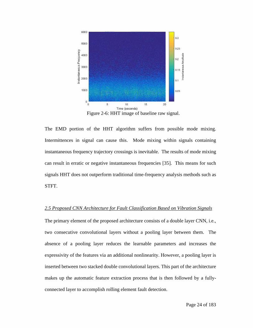
Figure 2-6 shows an HHT image of the raw baseline signal used in Figure 2-3 and

Figure 2-4. It is not uncommon for the HHT instantaneous frequencies to return

negative values. This is because the HHT derives the instantaneous frequencies from

the local derivatives of the IMF phases. The phase is not restricted to monotonically

increasing and can therefore decrease for a time. This results in a negative local

derivative. For further information regarding this property of HHT, the reader is

directed to read [34].

of 183

Figure 2-6: HHT image of baseline raw signal.

The EMD portion of the HHT algorithm suffers from possible mode mixing.

Intermittences in signal can cause this. Mode mixing within signals containing

instantaneous frequency trajectory crossings is inevitable. The results of mode mixing

can result in erratic or negative instantaneous frequencies [35]. This means for such

signals HHT does not outperform traditional time-frequency analysis methods such as

STFT.

2.5 Proposed CNN Architecture for Fault Classification Based on Vibration Signals

The primary element of the proposed architecture consists of a double layer CNN, i.e.,

two consecutive convolutional layers without a pooling layer between them. The

absence of a pooling layer reduces the learnable parameters and increases the

expressivity of the features via an additional nonlinearity. However, a pooling layer is

inserted between two stacked double convolutional layers. This part of the architecture

makes up the automatic feature extraction process that is then followed by a fully-

connected layer to accomplish rolling element fault detection.

of 183

The first convolutional layer consists of 32 feature maps of 3x3 size and followed by

second convolutional layer of 32 feature maps of 3x3 size. After this double

convolutional layer, there is a pooling layer of 32 feature maps of 2x2 size. This makes

up the first stage. The second stage consists of two convolutional layers of 64 feature

maps each, of 3x3 size, and followed by subsampling layer of 64 feature maps of 2x2

size. The third stage consists of two convolutional layers of 128 feature maps each, of

3x3 size, and followed by subsampling layer of 128 feature maps of 2x2 size. The last

two layers are fully connected layers of 100 features. Figure 7 depicts this architecture.

The intent of two stacked convolutional layers before a pooling layer is to get the

benefit of a large feature space via smaller features. This convolutional layer stacking

has two advantages: 1) reduces the number of parameters the training stage must learn,

and 2) increases the expressivity of the feature by adding an additional non-linearity.

Figure 2-7: Proposed CNN architecture.

Table 2-1 provides an overview of CNN architectures that have been used for fault

diagnosis, where C’s are convolutional layers, P’s are pooling layers, and FC’s are fully

connected layers. The number preceding the C, P, and FC indicates the number of

of 183

feature maps used. The dimensions [3x3] and [2x2] indicate the pixel size of the

features.

Table 2-1: Overview of CNN architectures used for fault diagnosis.

Proposed Model CNN Architecture

Architecture 1 [4] Input[32×32] - 64C[3×3] - 64P[2×2] - 64C[4×4] - 64P[2×2] - 128C[3×3] - 128P[2×2] - FC[512]

Architecture 2 [22] Input[32x32] - 16C[3x3] - 16P[2x2] - FC[10]

Proposed Architecture

Input[32x32] - 32C[3x3] - 32C[3x3] - 32P[2x2] - 64C[3x3] - 64C[3x3] - 64P[2x2] - 128C[3x3] - 128C[3x3] - 128P[2x2] - FC[100] - FC[100]

Proposed Architecture

Input[96x96] - 32C[3x3] - 32C[3x3] - 32P[2x2] - 64C[3x3] - 64C[3x3] - 64P[2x2] - 128C[3x3] - 128C[3x3] - 128P[2x2] - FC[100] - FC[100]

[18] Input[32×32] - 5C[5×5] - 5P[2×2] - 10C[5×5] - 10P[2×2] - 10C[2×2] - 10P[2×2] - FC[100] - FC[50]

[20] Input[128] - 64C[41] - 64P[2] - 32C[41] - 32P[2] - FC[10 - 10]

Training the CNN involves the learning of all of the weights and biases present within

the architectures. These weights and biases are referred to as learnable parameters.

The quantity of learnable parameters for a CNN architecture can radically improve or

degrade the time to train of the model. Therefore, it is important to optimize the

learnable parameters by balancing training time versus prediction accuracy. Table 2-2

outlines the quantity of learnable parameters for the proposed CNN architecture as well

as the a comparison to architectures 1 and 2 presented in Table 2-1.

Table 2-2: Overview of learnable parameters for the CNN architectures. CNN Model 32x32 Image 96x96 Image Architecture 2 41,163 368,854 Proposed CNN 501,836 2,140,236 Architecture 1 1,190,723 9,579,331

of 183

Beyond the learnable parameters, the CNN requires the specification and optimization

of the hyperparameters: dropout and learning rate. Dropout is an essential property of

CNNs. Dropout helps to prevent overfitting, reduce training error, and effectively thins

the network. The remaining connections are comprised of all the units that survive the

dropout. For this architecture, dropout is set to 0.5. For the other hyperparameter,

learning rate, the adapted moment estimation (ADAM) algorithm was used for

optimization. It has had success in the optimizing the learning rate for CNNs faster than

similar algorithms. Instead of hand-picking learning rates like similar algorithms, the

ADAM learning rate scale adapts through different layers [36].

Part of the reason for deep learning’s recent success has been the use of graphics

processing unit (GPU) computing [9]. GPU computing was used for this paper to

increase the speed and decrease the training time. More specifically, the processing

system used for the analysis are as follows: CPU Core i7-6700K 4.2 GHz with 32 GB

ram and GPU Tesla K20.

2.6 Case Study 1: Machinery Failure Prevention Technology (MFPT)

This data set was provided by the Machinery Failure Prevention Technology (MFPT)

Society [37], [38]. A test rig with a NICE bearing gathered acceleration data for

baseline conditions at 270lbs of load and a sampling rate of 97,656 Hz for six seconds.

In total, ten outer-raceway and seven inner-raceway fault conditions were tracked.

Three outer race faults included 270lbs of load and a sampling rate of 97,656 Hz for

six seconds. Seven additional outer race faults were assessed at varying loads: 25, 50,

of 183

100, 150, 200, 250 and 300 lbs. The sample rate for the faults was 48,828 Hz for three

seconds. Seven inner race faults were analyzed with varying loads of 0, 50, 100, 150,

200, 250 and 300 lbs. The sample rate for the inner race faults was 48,848 Hz for three

seconds. Spectrogram, Scalogram, and HHT images were generated from this data set

with the following classes: normal baseline (N), inner race fault (IR), and outer race

fault (OR). The raw data consisted of the following data points: N with 1,757,808 data

points, IR with 1,025,388 data points, and OR with 2,782,196 data points. The total

images produced from the data set are as follows: N with 3,423, IR with 1,981, and OR

with 5,404.

From MFPT, there was more data and information on the outer race fault conditions,

therefore more images were generated. This was decided due to the similarities

between the baseline images and the outer race fault images as shown in Tables 5 and

7. It is important to note that functionally the CNN looks at each pixel’s intensity value

to learn the features. Therefore, based on size and quantity, the 96x96 pixel and 32x32

pixel images result in 99,606,528 and 11,067,392 data points respectively.

Once the data images were generated, bilinear interpolation [39] was used to scale the

image down to the approriate size for training the CNN model. From this image data a

70/30 split was used for the training and test sets. These images are outlined in Table

2-3, Table 2-4, and Table 2-5.

of 183

Table 2-3: MFPT baseline images. Image Size

(Pixels) Spectrogram Scalogram HHT

32x32

96x96

Table 2-4: MFPT inner race images. Image Size


32x32

96x96

Table 2-5: MFPT outer race images. Image Size


32x32

96x96

of 183

Within the MFPT image data set, a few things stand out. Although, the scalogram

images of the outer race faults versus the baseline are similar, the scalogram images

had the highest prediction accuracy from all the modeling techniques employed in

Table 2-6 and Table 2-7. The information loss of the HHT images when reducing the

resolution from 96x96 to 32x32 pixels could be relevant because of the graphical

technique used to generate the images.

Depending upon the modeling technique used, the prediction accuracies are higher or

lower in Table 2-6 and Table 2-7. The CNN modeling had a significant shift between

96 and 32 image resolutions. Support vector machines (SVM) had a difficult time

predicting the faults for both the raw data (flat pixel intensities) and principal

component analysis (PCA).

Table 2-6: Prediction accuracies for 32x32 pixel image inputs.

Model Spectrogram Scalogram HHT MLP – Flat 70.3% 94.0% 49.2% LSVM – Flat 63.6% 91.8% 50.0% SVM – Flat 73.9% 92.7% 58.5% MLP – PCA 62.3% 95.3% 56.7% LSVM – PCA 48.8% 89.9% 45.8% SVM – PCA 51.3% 92.5% 56.4% Architecture 2 77.3% 92.4% 68.9% Architecture 1 80.6% 99.8% 74.5% Proposed CNN Architecture 81.4% 99.7% 75.7%

of 183

Table 2-7: Prediction accuracies for 96x96 pixel image inputs. Model Spectrogram Scalogram HHT

MLP – Flat 80.1% 81.3% 56.8% LSVM – Flat 77.1% 91.9% 52.8% SVM – Flat 85.1% 93.3% 57.8% MLP – PCA 81.5% 96.4% 69.2% LSVM – PCA 74.1% 92.0% 51.4% SVM – PCA 49.6% 70.0% 68.8% Architecture 2 81.5% 97.0% 74.2% Architecture 1 86.2% 99.9% 91.8% Proposed CNN Architecture 91.7% 99.9% 95.5%

Flat pixel data versus PCA of the pixel intensities varied across different modeling and

image selection. Scalograms outperformed spectrograms, and HHT. However, the

optimal modeling method using traditional techniques varied. For both the HHT and

spectrogram images, SVM on the flat data was optimal. For scalograms, MLP on the

PCA data was optimal.

Resolution loss from the reduction in image from 96x96 to 32x32 influenced the fault

diagnosis accuracies. There was a slight drop in the scalogram accuracies between the

two images sizes except for SVM PCA modeling. Spectrograms suffered a little from

the resolution drop; however, HHT was most affected. This is due to the image creation

method. Scatter plots were used due to the point estimates of the instantaneous

frequencies and amplitudes.

With regards to the CNN architectures, the proposed deep architecture outperformed

the shallow one. The shallow CNN architecture outperformed the traditional

classification methodologies in the 96x96 image sizes except for spectrograms. With

a 32x32 image size, the shallow CNN outperformed the traditional methods except for

of 183

the scalogram images. The proposed CNN architecture performed better overall for

the four different image techniques and resolution sizes except for 32x32 scalograms.

To measure the similarity between the results of the proposed CNN architecture versus

architectures 1 and 2, the model accuracies were compared with a paired two tail t-test.

Table 2-8 outlines the p-values with a null hypothesis of zero difference between the

accuracies. A p-value above 0.05 means the results are statistically the same. A p-

value less than 0.05 indicates the models are statistically distinct.

Table 2-8: MFPT paired two-tailed t-test p-values.

Architecture 1 Architecture 1 Architecture 2 Architecture 2 Image Type 32x32 96x96 32x32 96x96 Scalogram 0.080 0.344 0.049 0.108 Spectrogram 0.011 0.037 0.058 0.001 HHT 0.031 0.410 0.000 0.000

From the results in Table 2-8, one can see that the proposed architecture has the

advantage of outperforming or achieving statistically identical accuracies with less than

half the amount of the learnable parameters. Table 2-9 outlines the confusion matrices

results for the MFPT data set on 96x96 and 32x32 scalograms. The values are

horizontally normalized by class. From this, the following four metrics were derived:

precision, sensitivity, specificity, and F-measure (see [40] for details on these metrics).

of 183

Table 2-9: Confusion matrices for MFPT (A) 96x96 and (B) 32x32 scalograms for the proposed architecture.

N IR OR

N 99.9% 0.0% 0.1%

IR 0.0% 100% 0.0%

OR 0.1% 0.0% 99.9%

(A)

N IR OR

N 99.6% 0.1% 0.3%

IR 0.0% 100% 0.0%

OR 0.5% 0.0% 99.5%

(B)

Table 2-10: Precision for MFPT data set.

Model Proposed CNN Architecture

Architecture 1 Architecture 2

Scalogram 32x32 99.7% 99.8% 91.9% Scalogram 96x96 99.9% 99.9% 95.8% Spectrogram 32x32 82.0% 81.4% 78.8% Spectrogram 96x96 91.3% 85.0% 81.7% HHT 32x32 75.9% 74.6% 71.0% HHT 96x96 92.9% 89.7% 74.1%

Table 2-11: Sensitivity for MFPT data set.




Table 2-12: Specificity for MFPT data set.




34

Table 2-13: F-Measure for MFPT data set.




From the results shown in Table 2-10, Table 2-11,

Table 2-12, and Table 2-13, the precision, sensitivity, specificity, and f-measures of the

proposed architecture outperforms the other two CNN architectures when dealing with

spectrograms and HHT images of both 96x96 and 32x32 sizes and is statistically

identical to architecture 1 in case of scalograms. Precision assessments are beneficial

for diagnostics systems as it emphasizes false positives, thus evaluating the model’s

ability to predict actual faults. To measure the precision for the model, one must look

at each class used in the model. For the MFPT data set, three classes were used. Table

2-10 outlines the average precision of the three classes for the three architectures.

Sensitivity is another effective measure for a diagnostic system’s ability to classify

actual faults. However, sensitivity emphasizes true negatives. Table 2-11 outlines the

average sensitivity of the three classes. Specificity, or true negative rate, emphasizes

false positives, and is therefore effective for examining false alarm rates.

Table 2-12 outlines the average specificity. The f-measure metric assesses the balance

between precision and sensitivity. It does not take true negatives into account and

35

illustrates a diagnostic system’s ability to accurately predict true faults. Table 2-13

outlines the average f-measure for the three classes.

Overall, the proposed architecture outperforms or is statistically identical to the other

CNN architectures for diagnostic classification tasks with far fewer learnable

parameters. As shown from the images, the MFPT data set appears like it has more

noise in the measurements from the baseline and outer race fault conditions. Under

these conditions, the proposed architecture outperforms the other architectures due to

the two convolutional layers creating a more expressive non-linear relationship from

the images. Additionally, the proposed CNN can better classify outer race faults versus

the baseline (normal) condition even with very similar images.

2.7 Case Study 2: Case Western Reserve (CWR) University Bearing Data Center

The second experimental data set used in this paper was provided by Case Western

Reserve (CWR) University Bearing Data Center [6]. A two horsepower Reliance

electric motor was used in experiments for the acquisition of accelerometer data on

both the drive end and fan end bearings, as shown in Figure 2-8. The bearings support

the motor shaft. Single point artificial faults were seeded in the bearing’s inner raceway

(IR), outer raceway (OR), and rolling element (ball) (BF) with an electro-discharge

machining (EDM) operation. These faults ranged in diameter and location of the outer

raceway. The data includes a motor load of 0 to 3 horsepower. The accelerometers

were magnetically attached to the housing at the 12 o’clock position.

36

Figure 2-8: Test stand for roller bearing accelerometer data.

For the purposes of this paper, the speed and load on the motor were not included as a

classifier. Additionally, the fault sizes were grouped together as predicting the size of

the fault was beyond the scope of this paper. A 70/30 split was used for the training

and test data. Spectrogram, Scalogram, and HHT images were generated from this

data. The raw data consisted of the following data points: N had 1,691,648, BF had

1,441,792, IR had 1,440,768, and OR had 1,443,328 data points. The total images

produced from the data set are as follows: N 3,304, BF 2,816, IR 2,814, and OR 2,819.

From CWR, there was more balanced set of data between the baseline and faults.

Again, based on size and quantity, the 96x96 and 32x32 images result in 108,315,648

and 12,035,072 data points respectively. This data is used by the CNN to learn the

features of the data.

Deep learning algorithms hold promise to unlock previously unforeseen relationship

within explanatory variables; however, it is important to keep this in context. The value

of these algorithms is as much as they can outperform much simpler fault diagnosis

techniques. If envelope analysis, MLP, SVM or other traditional approaches can

achieve the same results, then there is no value in spending the extra time and resources

37

to develop a deep learning algorithm to perform the analysis. Smith et al [35] outlines

this benchmark study for the case western reserve data set for envelope analysis.

Appendix B within that paper outlines the potential areas within the data set where a

more sophisticated analysis must be used to diagnose certain faults. From these results,

analysis including the ball faults within the fault diagnosis requires more sophisticated

techniques. These include data sets 118 to 121, 185 to 188, 222, 224, and 225. These

data set are used within this paper; therefore, there is potential value to the

computational expense of the methodology proposed within this paper. These data sets

incorporated the small injected faults at 0.007” (data sets 118 to 121) to the larger

injected faults of 0.028” (data sets 3001 to 3004).

To be more explicit, the following data sets were used within the analysis. For the

baseline, data set 97 to 100. For the inner race, 105 to 108, 169 to 172, 209 to 212, and

3001 to 3004. For the ball faults, 118 to 121, 185 to 188, 222 to 225, and 3005 to 3008.

For the outer race faults, 130 to 133, 197 to 200, 234 to 237, and 144 to 147.

38

Bilinear interpolation [39] was used to scale the image down to the approriate size

for training the CNN model. A 70/30 split was used for the training and test sets. These

images are outlined in Table 2-14, Table 2-15,

Table 2-16, and

Table 2-17.

Table 2-14: CWR baseline images. Image Size Spectrogram Scalogram HHT

32x32

96x96

Table 2-15: CWR inner race images. Image Size Spectrogram Scalogram HHT

39

32x32

96x96

Table 2-16: CWR ball fault images. Image Size Spectrogram Scalogram HHT

32x32

96x96

Table 2-17: CWR outer race images. Image Size Spectrogram Scalogram HHT

32x32

96x96

The CWR image data set is different than the MFPT images. Even though the

scalogram images of the ball faults versus the inner race faults are similar, all four

40

image sets look easier to classify. The scalogram images had the highest prediction

accuracy for modeling techniques employed in Table 2-18 and Table 2-19. The

information loss of the HHT images when reducing the resolution from 96x96 to 32x32

did not affect the predictions as much as the MFPT data had, possibly due to the lower

noise levels in the case of the CWR data set.

Table 2-18: Prediction accuracies for 32x32 image inputs. Model Spectrogram Scalogram HHT


Table 2-19: Prediction accuracies for 96x96 image inputs. Model Spectrogram Scalogram HHT


Overall, spectrograms performed much better on the CWR data set then the MFPT data

set. Flat pixel data versus PCA of the pixel intensities varied across different modeling

and image selection. Spectrograms outperformed scalograms except for SVM PCA.

The optimal modeling method using traditional techniques varied. HHT’s optimal was

SVM PCA, spectrograms were SVM flat, and for scalograms, MLP PCA was optimal.

41

Like the MFPT results, resolution loss from the reduction in image from 96x96 to

32x32 influenced the classification accuracies. Like the MFPT results, there was a

slight drop in the scalogram accuracies between the two images sizes except for SVM

PCA modeling. All methods suffered a little from the resolution drop; however, HHT

again was the most affected.

The proposed architecture either outperformed or had statistically identical results with

the other architectures. Table 2-20 outlines the results of the t-test values for the CWR

data. The same hypothesis test as the MFPT data set was used for comparison.

Table 2-20: CWR paired two-tailed t-test p-values. Architecture 1 Architecture 1 Architecture 2 Architecture 2 Image Type 32x32 96x96 32x32 96x96 Scalogram 0.001 0.004 0.040 0.221 Spectrogram 0.022 0.000 0.000 0.211 HHT 0.005 0.784 0.000 0.000

Table 2-21 outlines the confusion matrix results for the CWR data set on 96x96

scalograms. The values are horizontally normalized by class. From this, the following

four tables of metrics were derived.

Table 2-21: Confusion matrix for CWR (A) 96x96 and (B) 32x32 scalograms for

the proposed architecture

N BF IR OR

N 98.4% 0.6% 0.0% 1.0%

BF 0.0% 99.8% 0.0% 0.2%

IR 0.0% 0.0% 100% 0.0%

42

OR 0.2% 0.0% 0.0% 99.7%

(A)

N BF IR OR

N 97.0% 2.0% 0.0% 1.0%

BF 0.5% 99.1% 0.0% 0.3%

IR 0.0% 0.0% 100% 0.0%

OR 0.6% 0.6% 0.0% 98.8%

(B)

Table 2-22: Precision for CWR data set.




Table 2-23: Sensitivity for CWR data set.




Table 2-24: Specificity for CWR data set.




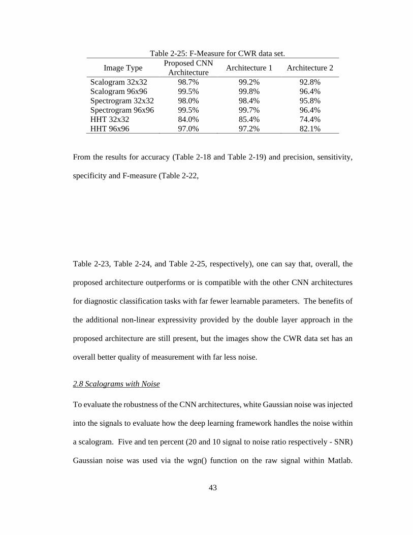
43

Table 2-25: F-Measure for CWR data set.

Image Type Proposed CNN Architecture



From the results for accuracy (Table 2-18 and Table 2-19) and precision, sensitivity,

specificity and F-measure (Table 2-22,

Table 2-23, Table 2-24, and Table 2-25, respectively), one can say that, overall, the

proposed architecture outperforms or is compatible with the other CNN architectures

for diagnostic classification tasks with far fewer learnable parameters. The benefits of

the additional non-linear expressivity provided by the double layer approach in the

proposed architecture are still present, but the images show the CWR data set has an

overall better quality of measurement with far less noise.

2.8 Scalograms with Noise

To evaluate the robustness of the CNN architectures, white Gaussian noise was injected

into the signals to evaluate how the deep learning framework handles the noise within

a scalogram. Five and ten percent (20 and 10 signal to noise ratio respectively - SNR)

Gaussian noise was used via the wgn() function on the raw signal within Matlab.

44

Additionally, the noisy images were randomly sampled without replacement to

generate a 50:50 mix with images of the raw signal (zero noise). The MFPT data set

was chosen for this analysis as it had a higher amount of noise in the baseline and outer

race images. Examples of those images can be seen in Table 2-26.

Table 2-26: MFPT 96x96 scalogram images with noise injected. Data Set Baseline 5% Noise 10% Noise

Normal

Inner Race

Outer Race

From these images the models were trained and assessed. Those results can be found

in Table 2-27. Both architectures 1 and 2’s prediction accuracy suffered from the

injection of noise. This is due in part to only having one convolutional layer before

pooling, therefore limiting the richness of the features for the final predictions. The

inclusion of an additional convolutional layer within the proposed architecture prior to

the pooling layer results in a much richer feature and the increased non-linearity helps

the architecture handle noise better than the other architectures here examined.

45

Table 2-27: Prediction accuracies for MFPT scalograms with injected noise.

Noisy Image Set Architecture 2 Architecture 1 Proposed CNN Architecture

96x96 w/ 5% Noise 96.6% 99.9% 99.9% 96x96 w/ 10% Noise 88.6% 91.8% 99.9%

2.9 Traditional Feature Extraction

To have a direct comparison with the standard fault diagnostic approach that relies on

manually extracted features, we now examine the use of extracted features as an input

to the CNN architectures discussed in this paper. The architectures were modified

slightly to accommodate the vector inputs; however, the double convolutional layer

followed by a pooling layer architecture was kept intact.

2.9.1 Description of Features

The vibration signals were divided in bins of 1024 samples each with an overlapping

of 512 samples. Each of these bins was further processed to extract the following

features from the original, derivative and integral signals: maximum amplitude, root

mean square (RMS), peak-to-peak amplitude, crest factor, arithmetic mean, variance

(σ2), skewness (normalized 3rd central moment), kurtosis (normalized 4th central

moment) and fifth to eleventh normalized central moments. Additionally, the

arithmetic mean of the Fourier spectrum, divided in 25 frequency bands along with the

RMS of the first five IMFs (Empirical Mode Decomposition) were used as features. In

total, seventy-five features per bin were computed and each of the features was

normalized using the mean and standard deviation of the first baseline condition.

46

2.9.2 Application to CNN Architecture

To evaluate the full set of features, the architecture of the CNN was changed slightly

to incorporate all the features. The following iteration of the proposed architecture was

used: Input[75x15] - 32C[75x3] - 32C[1x3] - 32P[2x2] - 64C[1x3] - 64C[1x3] -

64P[2x2] - FC[100]. Three different scenarios were examined: 1) twenty epochs with

early stopping and a stride of fifteen time steps with an overlap of eight times steps, 2)

thirty epochs with no early stopping and stride of fifteen time steps with an overlap of

eight times steps, and 3) twenty epochs with a stride of fifteen time steps with no

overlap.

Table 2-28 and Table 2-29 illustrate the difficulties the CNN architectures had when

dealing with the manually constructed features: the prediction accuracies considerably

dropped for all the CNN architectures for both MFPT and CWR data sets. Additional

epochs without early stopping improved the results; however, they are still well below

the results of the image representations. For the MFPT data, early stopping and data

overlap helped the accuracies. For the CWR data, the opposite is true for early

stopping. The CWR data benefited from more epochs; however, the MFPT data

suffered slightly from increased epochs.

Table 2-28: Prediction accuracies for CWR.

Model 20 Epochs Early Stopping

30 Epochs No Early Stopping

No Overlap

Architecture 2 75.2% 86.7% 67.2% Architecture 1 90.4% 95.7% 87.2% Proposed CNN Architecture 83.1% 98.5% 93.6%

47

Table 2-29: Prediction accuracies for MFPT. Model 20 Epochs

Early Stopping 30 Epochs No Early Stopping

No Overlap

Architecture 2 79.1% 80.9% 75.2% Architecture 1 82.9% 75.1% 75.1% Proposed CNN Architecture 96.4% 93.8% 87.3%

The CNN strength is images and it has spatial awareness; therefore, the ordering of the

features within the vector could influence the output predictions. It should be said that

the size of the vectors and filters were chosen on the input and convolutional layers to

minimize this effect.

CNNs are very good when the data passed through them is as close to the raw signal as

possible, as the strength of the convolutional and pooling are their ability to learn

features which are inherent representation of the data. If one manipulates the data too

much by engineering features in the traditional sense, the CNNs do not perform as well.

As illustrated from the results in Table 2-28 and Table 2-29, the CNN architectures had

difficulties in all scenarios. Moreover, even in this unfavorable scenario, the proposed

architecture outperformed the others. The stacked convolutional layers, as in the case

with infused noise, result in more expressive features to better capture the non-linearity

of the data. Thus, one can argue that for CNNs, it is optimal to use an image

representation of the raw signal instead of a vector of extracted features.

2.10 Concluding Remarks

Fault diagnosis of rolling element bearing is a significant issue in industry. Detecting

faults early to plan maintenance is of great economic value. Prior applications of deep

48

learning-based models tended to be limited by their sensitivity to experimental noise or

their reliance on traditional feature extraction. In this paper, a novel CNN architecture

was applied to the time-frequency and image representations of raw vibration signals

for use in rolling element bearing fault classification and diagnosis. This was done

absent the need for traditional feature extraction and selection and to exploit the deep

CNNs strength for fault diagnosis: automatic feature extraction.

To determine the ability for the proposed CNN model to accurately diagnose a fault,

three time-frequency analysis methods (STFT, WT, and HHT) were compared. Their

effectiveness as representations of the raw signal were assessed. Additionally,

information loss due to image scaling was analyzed which had little effect on the

scalogram images, a slight effect on the spectrograms, and larger effect on the HHT

images. In total, 189,406 images were analyzed.

The proposed CNN architecture showed it is robust against experimental noise.

Additionally, it showed featureless learning and automatic learning of the data

representations were effective. The proposed architecture delivers the same accuracies

for scalogram images with lower computational costs by reducing the number of

learnable parameters. The architecture outperforms similar architectures for both

spectrograms and HHT images. The manual process of feature extraction and the

delicate methods of feature selection can be substituted with a deep learning framework

allowing automated feature learning, therefore removing any confirmation biases

surrounding one’s prior experience. Overall, the CNN transformed images with

49

minimal manipulation of the signal and automatically completed the feature extraction

and learning resulting in a much-improved performance.

Fault diagnosis is a continually evolving field that has vast economic potential for

automotive, industrial, aerospace, and infrastructure assets. One way to eliminate the

bias and requirement of expert knowledge for feature extraction and selection is to

implement deep learning methodologies which learn these features automatically.

Industries could benefit from this approach on projects with limited knowledge, like

innovative new systems.

Acknowledgments

The authors acknowledge the partial financial support of the Chilean National Fund for

Scientific and Technological Development (Fondecyt) under Grant No. 1160494.

50

Chapter 3: Unsupervised Deep Generative Adversarial Based Methodology for Automatic Fault Detection2

3.1 Abstract

System health management is of upmost importance with today’s sensor integrated

systems where a constant stream of data feeds information about a system’s health is

available. Traditional methods to assess this health focus on supervised learning of

these fault classes. This requires labeling sometimes millions of points of data and is

often laborious to complete. Additionally, once the data is labeled, hand-crafted feature

extraction and selection methods are used to identify which are indicators of the fault

signals. This process requires expert knowledge to complete. An unsupervised

generative adversarial network-based methodology is proposed to address this

problem. The proposed methodology comprises of a deep convolutional generative

adversarial network (GAN) for automatic high-level feature learning as an input to

clustering algorithms to predict a system’s faulty and baseline states. This methodology

was applied to a public data set of rolling element vibration data from a rotary

equipment test rig. Wavelet transform representations of the raw vibration signal were

used as an input to the deep unsupervised generative adversarial network-based

methodology for fault classification. The results show that the proposed methodology

is robust enough to predict the presence of faults without any prior knowledge of their

signals.

2 The full-text of this chapter has been published at Verstraete, D. B., et al. "Unsupervised deep generative adversarial based methodology for automatic fault detection." Safety and Reliability–Safe Societies in a Changing World. CRC Press, 2018. 1051-1056.

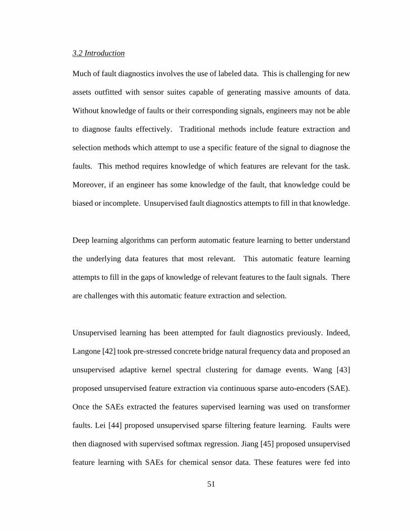
51

3.2 Introduction

Much of fault diagnostics involves the use of labeled data. This is challenging for new

assets outfitted with sensor suites capable of generating massive amounts of data.

Without knowledge of faults or their corresponding signals, engineers may not be able

to diagnose faults effectively. Traditional methods include feature extraction and

selection methods which attempt to use a specific feature of the signal to diagnose the

faults. This method requires knowledge of which features are relevant for the task.

Moreover, if an engineer has some knowledge of the fault, that knowledge could be

biased or incomplete. Unsupervised fault diagnostics attempts to fill in that knowledge.

Deep learning algorithms can perform automatic feature learning to better understand

the underlying data features that most relevant. This automatic feature learning

attempts to fill in the gaps of knowledge of relevant features to the fault signals. There

are challenges with this automatic feature extraction and selection.

Unsupervised learning has been attempted for fault diagnostics previously. Indeed,

Langone [42] took pre-stressed concrete bridge natural frequency data and proposed an

unsupervised adaptive kernel spectral clustering for damage events. Wang [43]

proposed unsupervised feature extraction via continuous sparse auto-encoders (SAE).

Once the SAEs extracted the features supervised learning was used on transformer

faults. Lei [44] proposed unsupervised sparse filtering feature learning. Faults were

then diagnosed with supervised softmax regression. Jiang [45] proposed unsupervised

feature learning with SAEs for chemical sensor data. These features were fed into

52

supervised softmax regression to diagnose faults. Sun [46] took induction motor fault

data and proposed the use of SAEs for unsupervised feature extraction. These features

were again followed by supervised learning for classification by neural networks (NN).

Of these approaches, only Langone et al could be considered truly unsupervised. The

rest are restricted to unsupervised feature learning followed by supervised fault

diagnostics. Moreover, apart from the use of SAEs, none of these methods would be

considered deep.

In this paper, we propose a GANs based methodology application to unsupervised fault

diagnostics on scalogram image representations. To validate the proposed

methodology, the public Machinery Failure Prevention Technology (MFPT) Society

bearing data set [37], [38] is used. To evaluate the proposed unsupervised methodology,

traditional supervised learning metrics cannot be used. A confusion matrix and its

associated measures are unable to evaluate clustering techniques. Therefore, since the

ground truth is known, external validation measures purity, normalized mutual

information (NMI), and adjusted rand index (ARI) are used to evaluate the quality of

the clusters. The remainder of this paper is structures as follows. Section 2 gives an

overview of GANs and the methodology. Section 3 presents results of the GANs based

methodology applied to the MFPT data set. Section 4 provides conclusions.

3.3 Generative Adversarial Networks

Generative adversarial networks (GANs) have at their core a minimax game which

seeks to pit a forger, the generator network, against a detective, the discriminator

53

network. The generator seeks to create fake data, or scalograms in this paper, to trick

the discriminator who must discriminate between the real data and the fake data as

shown in Figure . Back propagation is performed on the weights and biases and the

process is repeated. The benefit to this training is while the generator seeks to develop

an underlying distribution of the real data, the discriminator is feeding information back

to the generator, not on the real data, on the weights and biases of the learned features.

This helps to prevent overfitting of the data.

Z ~ N(μ,σ)

Fake Images X' Real Images X

Generator

Discriminator

Ba

ck Prop

ag

ation

**Insert

Fake Images

here**

Fake or Real? Figure 3-1: GAN Training

Within this minimax game, the objective function to maximize the value, V, to the point

where the discriminator and generator no longer find it necessary to make changes to

their weights and biases. While this is the goal of GAN training, there is functionally

no mechanism with the training to control it. Therefore, there can be issues with

convergence. More formally in Eq. (5) from [47]:

54

minT max U V�W, X�= YZ~\]^_^�Z�`log �X�x�b+ Yc~\defgh�c�`log �1 − X�W�z��b (5)

where, Pdata�x� is the data distribution, Pnoise�x� is the noise distribution, D�x� is the Discriminator objective function, and G�z� is the generator objective function.

The GANs based methodology used in this paper can be found in Figure 3-2. The

methodology starts with developing a scalogram image representation of the raw data,

and then proceeds to training of the deep convolutional generative adversarial network

(DCGAN). Once the DCGAN training is completed and visual inspection of the

generator output images is done, concatenation of the last activation layer of the

discriminator is completed. Once the activations are concatenated, kmeans++ is used

for clustering on the first two principal components. Visual inspection of the generator

output is still needed within GANs training and is a crucial step within the training.

55

GANs Unsupervised Learning

GANs Discriminator

Raw Signal StartScalogram Representation

End

Real Images X

GANs Generator

Z ~ N(μ,σ)

Fake Images X’

Back Propagation

DCGAN

Concatenate Last Convolutional Activations

PCA/Kmeans++

Figure 3-2: Proposed Unsupervised GAN Methodology

There are two goals for the output of this methodology: 1) Separation of the baseline

healthy data with the fault data, and 2) Separation of the individual faults. When a new

sensor system comes online, the engineer needs to know when the system drifts from

healthy signals to a signal with which to decide when to conduct planned maintenance.

Once the engineer has familiarity with the system and signals can be identified as

individual faults on the inner or outer raceway, then better predictions and a fully

supervised methodology can be used [48].

The GAN architecture used in this paper incorporates the guidelines proposed in

Radford [49]; however, adjustments to that paper’s architecture were made for handling

the MFPT data set. Radford et al provides the following five GANs architecture

guidelines: 1) generator and discriminator network pooling layer replacement with

56

strided convolutions, 2) Batch normalization (BN) is required for both the discriminator

and generator networks, 3) Fully connected hidden layers should be removed for deep

architectures, 4) Rectified Linear Unit (ReLU) activation use in all layers of the

generator except the output should use Tanh, and 5) Leaky ReLU activation use on all

layers for the discriminator. DCGANs are used in this paper as a baseline to implement

GANs. The combination of these five guidelines composes what is defined as deep

convolutional generative adversarial networks (DCGANs).

3.3.1 Strided Convolutions

The relationship between a convolutional operation’s input shape, i j, and the

operation’s output shape, oj, of a convolutional layer along axis j are related to three

factors: 1) kernel size (kj), 2) stride (sj), and 3) padding (pj). Convolutional strides are

generally set to �o = 1 for most operations; however, for GANs strided convolutions

of �o > 1 are used in place of pooling layers. This is applied for the discriminator to

learn its own downsampling, and for the generator to learn its own upsampling.

3.3.2 Batch Normalization

Batch normalization (BN) is an important addition to the architecture between each

convolutional layer [50]. As the data moves through the convolutional layers the weight

and bias values are adjusted. This has the potential to lead to the data increasing or

decreasing to unrealistic values. Batch normalization prevents this from becoming an

issue with the training by normalizing the data to a mean of zero and a variance of one

for each data batch. Setting values of x over a mini-batch: + = q�%…..�t to output the

57

learned parameters γ and β, uvF = BNy,z��F�{. The min-batch mean is |z ← %� ∑ �F�F(% ,

the mini-batch variance is �z5 ← %� ∑ ��F − |z�5�F(% , they are then normalized with ��F ←�f$��@�E9�, and scale and shifted with, vF ← ��F + + ≡ ��y,z��F�.

3.3.3 Activation Layers

The following activation functions are used throughout the architecture. For the

generator two activations functions are used: 1) Rectified Linear Unit (ReLU), f�x� =�0forx < 0xforx ≥ 0 and 2) Hyperbolic tangent (tanh). Within the generator network ReLU is

used between every layer except tanh activation is used after the last layer. For the

discriminator, Leaky ReLU is used on every layer. Leaky ReLU differs from ReLU in

values less than 0.

3.3.4 Neural Network Architectures

The neural network architectures used in the proposed methodology incorporate the

guidelines as proposed by Radford et al. Two networks were developed to account for

the data set presented in this chapter. The generator network, as shown in Figure 3-3,

takes the vector of noise and through deconvolution, BN and activation functions

creates an image. In this case the output if a 96x96 image of a scalogram of a signal.

To do this, a 100x1 vector is projected and reshaped to deconvolve into a 6x6x512

feature space. This space is then deconvolved to a 12x12x256, then 24x24x128,

48x48x64, and finally a 96x96x3 image.

58

96x96 Image6x6x512 100 z

Project and

Reshape

12x12x256 24x24x128 48x48x64 96x96x3

Dec

onvo

lutio

n

DC

DC

DC

DC

BN

BN

BN

BN

BN

Re

LU

Re

LU

Re

LU

Re

LU

Ta

nh

Figure 3-3: Generator Network

96x96 Image

Con

volu

tion

BN

Leak

y R

eLU

Con

volu

tion

BN

Leak

y R

eLU

Con

volu

tion

BN

Leak

y R

eLU

Con

volu

tion

BN

Leak

y R

eLU

6x6x512 12x12x256 24x24x12848x48x64

Figure 3-4: Discriminator Network

The discriminator network, as shown in Figure 3-4, then takes that generated image

and judges whether the image is real or fake. It does this by taking the real images and

automatically learning the feature subspace. For the 96x96 images this results in a

network of convolutional layers consisting of a 48x48x64 layer, 24x24x128,

12x12x256, and 6x6x512 layers. The output of this last activation holds a lot of

information about the feature space and is useful for unsupervised fault diagnostics.

3.4 Propose Methodology Application

The MFPT data set is a good test of any algorithm as the outer race fault and baseline

conditions are difficult to separate. NICE bearings were used within an experimental

test rig. Accelerometer data was gathered on three conditions. First, at a sampling rate

of 97,656 Hz, a baseline condition at 270lbs of load was captured. Second, a total of

ten faults on the outer-raceway were gathered. At the same sampling rate and loading

condition as the baseline, three outer race faults were tested, and the remaining seven

59

outer race faults had the following load cases: 25, 50, 100, 150, 200, 250 and 300

lbs. These seven load cases had a sampling rate of 48,828 Hz. Third, with a sampling

rate again of 48,848 Hz, seven inner race faults at a loading of 0, 50, 100, 150, 200,

250 and 300 lbs were gathered. From these raw signals, scalogram image

representations were created with the following three classes as shown in

Table 3-: normal baseline (N), inner race fault (IR), and outer race fault (OR). In total

10,808 scalogram images were generated with 3,423 baseline, 1,981 inner race, and

5,404 outer race images. The training, validation, and test sets used were fifty percent,

twenty five percent, and twenty five percent of the full data set respectively. Bilinear

interpolation [39] aided in reducing the original images to down to a trainable size for

the GAN architecture.

Table 3-1: 96x96 pixel MFPT scalogram images. Baseline Inner Race Outer Race

The first step once the GANs training is completed is visual inspection of the generator

image outputs. These can be seen in Figure 3-5. The different fault conditions can be

identified within the images. This step is a key indicator for identification of mode

collapse, vanishing gradients, non-convergence, or checkerboarding artifacts. With

this completed the last activation layer of the discriminator network can be

concatenated and clustering can be done.

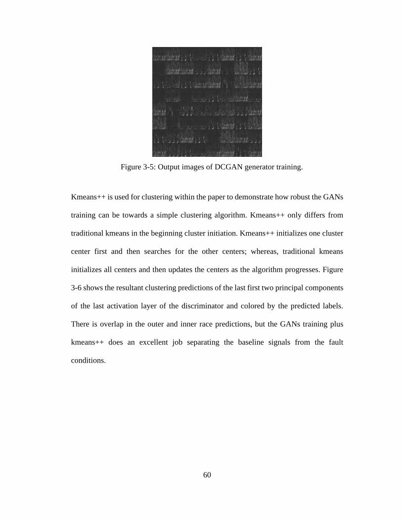
60

Figure 3-5: Output images of DCGAN generator training.

Kmeans++ is used for clustering within the paper to demonstrate how robust the GANs

training can be towards a simple clustering algorithm. Kmeans++ only differs from

traditional kmeans in the beginning cluster initiation. Kmeans++ initializes one cluster

center first and then searches for the other centers; whereas, traditional kmeans

initializes all centers and then updates the centers as the algorithm progresses. Figure

3-6 shows the resultant clustering predictions of the last first two principal components

of the last activation layer of the discriminator and colored by the predicted labels.

There is overlap in the outer and inner race predictions, but the GANs training plus

kmeans++ does an excellent job separating the baseline signals from the fault

conditions.

61

Figure 3-6: DCGAN PCA KMeans ++ predicted.

Figure 3-7 shows the first two principal components of the last activation layer color

coded by the real labels. It appears the GAN training with kmeans++ had the most

difficulty with separating the fault conditions. A clustering algorithm more capable of

handling the non-convex nature of the outer race fault could potentially increase the

evaluation metrics but is beyond the scope of this paper.

Figure 3-7: DCGAN PCA Kmeans ++ real.

62

Since the labels to the data are known, evaluation metrics like purity [51], normalized

mutual information (NMI) [52], and adjusted RAND index (ARI) [53] can be used to

validate the architecture. Table 3-2 has the overview of these metrics for this

methodology.

Table 3-2: MFPT 96x96 generator output, DCGAN, Kmeans++.

ARI Purity NMI 0.50 0.79 0.62

Overall these number could be improved; however, the first goal of this methodology

is to separate the baseline healthy system state with that of the faults. This methodology

proves it can handle that. More work can be done to improve these numbers and

provide better information to the engineer regarding which individual fault case the

signal is presenting itself as.

3.5 Conclusions

Generative adversarial networks and deep learning as a field stand to unlock numerous

potential applications within the field of engineering research. This application is the

first of its kind and shows great promise.

The proposed architecture demonstrates its abilities with automatic feature learning to

a level with which a simple clustering algorithm can separate the healthy baseline

signals with the fault data. An engineer can easily make an engineering decision on

maintenance without the need for any knowledge of the individual signals.

The practical application of this paper has far reaching possibilities into many

engineering fields and is not limited to rolling element bearings. Aerospace,

63

automotive, oil & gas, and many other industries can utilize this unsupervised

methodology.

Acknowledgments



64

Chapter 4: Deep Semi-Supervised Generative Adversarial Fault Diagnostics of Rolling Element Bearings.3

4.1 Abstract

With the availability of cheaper multi-sensor suites, one has access to massive and

multi-dimensional datasets that can and should be used for fault diagnosis. However,

from a time, resource, engineering, and computational perspective, it is often cost

prohibitive to label all the data streaming into a database in the context of big machinery

data, i.e., massive multidimensional data. Therefore, this paper proposes both a fully

unsupervised and semi-supervised deep learning enabled generative adversarial

network-based methodology for fault diagnostics. Two public data sets of vibration

data from rolling element bearings are used to evaluate the performance of the proposed

methodology for fault diagnostics. The results indicate that the proposed methodology

is a promising approach for both unsupervised and semi-supervised fault diagnostics.

4.2 Introduction

Condition health monitoring systems are becoming a standard specification for

customers purchasing large capital assets. With the proliferation of cheap sensing

technology, these assets are now streaming massive quantities of data at an

unprecedented rate. The fields of structural health monitoring (SHM) and fault

diagnostics have grown from the need to make sense of this data. The primary

3 The full-text of this chapter has been published at Verstraete, David Benjamin, et al. "Deep semi-supervised generative adversarial fault diagnostics of rolling element bearings." Structural Health Monitoring (2019): 1475921719850576.

65

drawback to fault diagnostics within these systems is the requirement of labeling

millions, and potentially billions, of data points. To label a data set of this magnitude

is resource intensive, costly, computationally expensive, and subject to confirmational

data biases of the engineers interpreting the data. Thus, labeling the output of an

extensive sensor system data output requires significant investment. Moreover, there is

a strong assumption within supervised fault diagnosis that everything is known about

a preset class of faults. This restricts the ability of the supervised model to generalize.

If the model only knows what the engineer knows, it is reasonable to assume the

model’s knowledge of the system could be incomplete; therefore, traditional feature

learning would have a fundamental generalization problem.

The general problem within unsupervised learning is extracting information or value

from unlabeled data. Unsupervised learning is an ill-posed problem because

appropriate downstream tasks are unknown at the time of training. Therefore,

unsupervised learning should disentangle the relevant unknown tasks which are helpful

for the problem. For instance, a useful disentangled representation for a dataset of

cracks in a concrete structure would be dimensions for crack length, crack width,

neighboring cracks, or the presence of the crack intersections [68]. These

representations may be relevant for natural tasks like damage evaluation or crack

propagation. For irrelevant tasks, like the percentage of white pixels, this

representation would be extraneous. Therefore, a useful unsupervised learning

algorithm must guess the likely set of subsequent classification tasks correctly without

knowledge of what the tasks are. This is a challenge deep learning attempts to solve.

66

Deep learning makes up much of the recent unsupervised fault diagnostic research,

[42], [43], [44], [69], [70], [71], [72], [73], and [74]. All these approaches, except

Langone [42], are restricted to unsupervised feature learning followed by supervised

fault diagnostics. Moreover, none of these methods attempt unsupervised learning with

an image representation of the data.

Most recently, Generative Adversarial Networks (GANs) have been developed within

the computer vision community [47]. Training this deep generative modeling is done

using a minimax game. The goal of training is to learn a generator distribution that

fools the discriminator into classifying it as from the true data distribution. Unlike

variational autoencoders (VAE), which tries to assign probability to every data point in

the data distribution [66], a GAN learns a generator network which transforms a noise

variable in a sample by generating samples from the sample distribution. With a

sharper image from GANs, one gets more precise image features. However, currently

there are no agreed upon methods to assess the training of, or comparison of, a GAN

without visually inspecting the images. This is difficult to accomplish without an

image of the signal. A vector of data would not suffice. Therefore, GANs provides a

better foundation for fault diagnostics based on rich images of signals.

In this paper we propose a novel deep learning generative adversarial methodology for

a comprehensive approach to fault diagnostics on time-frequency images. This paper

explores both deep convolutional GANs (DCGAN) and InfoGAN architectures. From

the proposed architectures for these two types of GANs networks, clustering is done

67

via spectral and kmeans++ clustering on the down-sampled activation output of the

discriminator. To improve clustering results, semi-supervised learning is included as a

second stage to the methodology by altering the cost function to account for data labels.

Additionally, both 32x32 pixel and 96x96 pixel images are explored as inputs to

methodology. This methodology is then evaluated with both the Machinery Failure

Prevention Technology (MFPT) Society [37] and Case Western Reserve (CWR)

University Bearing Data Center [6] bearing data sets. The proposed methodology’s

results are then compared to unsupervised learning via autoencoders (AE) and VAE.

To evaluate the proposed unsupervised methodology, traditional supervised learning

metrics are inappropriate. A confusion matrix and its associated metrics are unable to

evaluate clustering techniques. The ground truth is known; therefore, purity [51],

normalized mutual information (NMI) [52], and adjusted rand index (ARI) [53] are

used to evaluate the quality of the clusters.

The rest of this paper is organized as follows, Section 2 provides an overview of GANs.

Section 3 outlines the proposed unsupervised and semi-supervised methodology

constructed to aid the diagnostic task of fault detection. Section 4 applies the

methodology to both the MFPT and CWR experimental data sets. Section 5 compares

these results to unsupervised AE and VAE. Section 6 finishes with some concluding

remarks.

68

4.3 Background on Adversarial Training

Generative adversarial networks were first proposed by Goodfellow et al [47]. GANs

consist of a generator network and a discriminator model network. Generative models

seek to learn the underlying joint probability distribution P(x,y) of the random variables

to categorize a signal. Discriminative models, on the other hand, disregard how the

data was generated and simply categorize the data points based on a conditional

probability distribution p(y|x) [80]. Within the context of fault diagnostics, generative

models attempt to learn every potential fault to then classify the faults, whereas

discriminative models attempt to determine fault differences absent of learning every

fault. GANs seek to utilize both model’s strengths. The generator attempts to create a

synthetic data set, X’, that matches the real data, X, that only the discriminator can see

and classify as shown in Figure . The generator samples from a noise distribution, Z

(e.g. normal) and the discriminator determines whether the sampled data (e.g., an

image) is real or fake.

Z

Z ~ N(μ,σ)

Fake Images X'

Real Images X

Generator Network

Discriminator Network

D(X)

Figure 4-1: GAN overview.

69

Functionally, GANs train two convolutional neural networks at the same time. The

generator, which is depicted in Figure , utilizes deconvolutional layers to take the noisy

input Z and creates the specified size image. The parameters in Z is then updated

continuously throughout the training of the network. This image is then fed into the

discriminator network to judge whether the generated image is real or fake. The

discriminator is a convolutional neural network with convolutional layers, pooling, and

non-linear activations. This is all done in a feed forward operation where the weights,

biases, and errors are set throughout. To update the networks and adjust these

hyperparameters, backpropagation is used to send the errors back through the networks

to update the weights and biases. This process removes redundant, uninteresting

features.

To accomplish this, the fundamental foundation of the GANs algorithm is the two-

player minimax game. The generative network maps a noise source to an input space

to generate a fake image. The discriminative network receives the generators input (a

fake image) and classifies it as real or fake. This amounts to a two-player game with

the two networks competing against each other, Eq. (6) [47]:

minT max U V�W, X�= YZ~\]^_^�Z�`log �X�x�b+ Yc~\defgh�c�`log �1 − X�W�z��b (6)

Where, Pdata�x� Data distribution Pnoise�x� Noise distribution

70

D�x� Discriminator objective function G�z� Generator objective function

For each generator parameter update the discriminator is trained to optimality. The

minimization of the value function leads to the minimization of the Jensen-Shannon

(JS) divergence between the real data and the trained model distributions on x. This

minimization frequently results in vanishing gradients as the discriminator saturates.

While the ideal training results in optimality, in most practical applications this is not

necessarily the case. At the moment the training of GANs requires visual inspection

of the output images; therefore, an image representation of the signal is needed.

There has been, and there continues to be, a large amount of research surrounding the

architectures and training of a GAN. For this paper both DCGAN and InfoGAN are

used. Fundamentally, these two GAN are identically trained to the proposed method

by Goodfellow [47]. However, their architectures and cost functions are modified to

account for the applied data sets and unsupervised vs semi-supervised objective

functions.

4.3.1 Clustering

This paper examines two primary clustering algorithms for classification (k-means++

and spectral) and PCA for visualization. K-means++ was chosen to explore the

robustness of the methodology to simple clustering algorithms. K-means++ differs

from the traditional k-means algorithm by first choosing the initial cluster center

71

uniformly at random and then choosing each subsequent center with probability

proportional to the square of its proximity to the nearest center [75].

Algorithm 1 K-means++ algorithm Initialize k-means++ algorithm • Take one center, A%, chosen uniformly at random from data points, X.

• Take a new center, AF, choosing � ∈ � with probability U��E∑ U��E�∈� , where X��

denotes the shortest distance from a data point to the closest center already chosen. • Repeat previous step until all k centers are taken. • Proceed with standard k-means algorithm. Spectral clustering on the other hand is a graph clustering technique where eigenvectors

of the data matrices are used. Data is mapped to a low-dimensional space for spectral

clustering. This dimensionality reduction is more computationally expensive than the

k-means++ algorithm; however, it can achieve superior results [76].

Algorithm 2 Spectral clustering algorithm Input: Similarity matrix � ∈ ℝ�×�, number k of clusters to construct • Construct a similarity graph. Let W be its weighted adjacency matrix. • Compute the unnormalized Laplacian L. • Compute the first k eigenvectors �%, . . . , �� of the generalized eigenproblem �� =�X�. • Let V ∈ ℝ�×� be the matrix containing the vectors �%, . . . , �� as columns. • For � = 1, . . . , �, let vF ∈ ℝ� be the vector corresponding to the i-th row of V. • Cluster the points �vF�F(%,...,� in ℝ� with the k-means algorithm into clusters �%, . . . , ��. Output: Clusters �%, . . . , �� with �F = q�|vo ∈ �Ft.

4.4 Proposed Generative Adversarial Fault Diagnostic Methodology

A two-stage fault diagnostic methodology is proposed within this paper. Stage one

consists of fully unsupervised generative adversarial fault diagnostics, and stage two

semi-supervised generative adversarial fault diagnostics. In practice, sensor signals are

gathered, and stage one can be used at the start to assess the baseline of the system

72

when labels for the data are unavailable. As knowledge of the system signals improve,

fault signals can be identified, labeled, and then incorporated into stage two. The

intention is that unsupervised clustering, operating on the automatic identified features

by the GAN, identifies fault clusters away from the baseline. Once labeled data is

available it can be added to the model to improve the maintenance decision making.

Upon completion, the engineer can then visually monitor the system via principal

components analysis (PCA) to begin labeling some of the signals being gathered. This

labeled data can then be input into the GANs methodology, with a modification to the

cost function, to further improve the clustering results until a predefined criterion of

performance is met. Once the system signals move to a fully supervised labeled data

set, the engineer can then transition the modeling to a fully supervised deep learning

framework (for example, see [48]).

The discriminator network provides the ability to train itself against generated images

as an adversary within both DCGAN and InfoGAN architectures. Since the

discriminator is trained to predict the fake from the real dataset, it can provide a robust

feature set of the real data. To accomplish this, the GAN discriminator training

automatically generates a high-level feature representation of the data from the input

image to an output vector. The goal of the GANs training is then to take this high-level

representation feature set as an input to clustering algorithms. This allows the generator

to avoid overfitting on the raw data by only having access to the gradients. Two GAN

architectures explored in this paper are not a restriction on the methodology; these were

two architectures chosen because of their strong results in other tasks, such as image

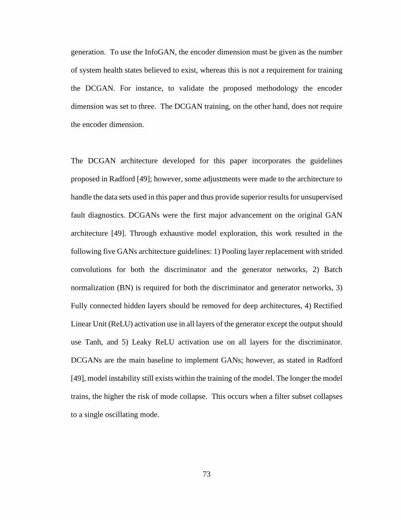
73

generation. To use the InfoGAN, the encoder dimension must be given as the number

of system health states believed to exist, whereas this is not a requirement for training

the DCGAN. For instance, to validate the proposed methodology the encoder

dimension was set to three. The DCGAN training, on the other hand, does not require

the encoder dimension.

The DCGAN architecture developed for this paper incorporates the guidelines

proposed in Radford [49]; however, some adjustments were made to the architecture to

handle the data sets used in this paper and thus provide superior results for unsupervised

fault diagnostics. DCGANs were the first major advancement on the original GAN

architecture [49]. Through exhaustive model exploration, this work resulted in the

following five GANs architecture guidelines: 1) Pooling layer replacement with strided

convolutions for both the discriminator and the generator networks, 2) Batch

normalization (BN) is required for both the discriminator and generator networks, 3)

Fully connected hidden layers should be removed for deep architectures, 4) Rectified

Linear Unit (ReLU) activation use in all layers of the generator except the output should

use Tanh, and 5) Leaky ReLU activation use on all layers for the discriminator.

DCGANs are the main baseline to implement GANs; however, as stated in Radford

[49], model instability still exists within the training of the model. The longer the model

trains, the higher the risk of mode collapse. This occurs when a filter subset collapses

to a single oscillating mode.

74

There have been many studies on the effectiveness of individual wavelets and their

ability to match a signal. One could choose between the Gaussian, Morlet, Shannon,

Meyer, Laplace, Hermit, or the Mexican Hat wavelets in both simple and complex

functions. To date there is not a defined methodology for identifying the proper wavelet

to be used and this remains an open question within the research community [30]. For

the purposes of this paper, the Morlet wavelet is chosen because of its similarity to the

impulse component of symptomatic faults of many mechanical systems [31].

As shown in Figure 4-2, the proposed methodology starts with the training of a GAN

with the unlabeled dataset. This will train two convolutional neural networks (CNNs),

one discriminator and one generator. The discriminator needs to learn distribution of

the real vibration fault dataset to be able to discriminate between the generated fake

samples and the real samples. The generator attempts to trick the discriminator by

learning the underlying distribution of the generated data. The last activation layer of

the training is then concatenated and visually inspected via PCA to evaluate the ability

of the GAN to separate the data. At this point the engineer will be looking for a robust

representation of the baseline signals from the asset. From there, the engineer weighs

the value of labeling the incoming data versus the cost to label.

75

GANs Unsupervised Learning(Algorithm 1)

GANs Discriminator

Increase % of labeled images

Start Labeling Data?

Label More Data?

Raw SignalStart

End

Yes

No

Yes

No

Real Images X

GANs Discriminator

Real Images X

DCGAN

GANs Generator

Z ~ N(μ,σ)

Fake Images X’

Back PropagationLunsupervised

GANs Semi-Supervised Learning

Clustering to Add Labels

GANs Generator

Fake Images X’

Z ~ N(μ,σ)

Back PropagationLsemi-supervised

Last Convolutional Activation Layer Concatenation

Clustering

Knowledge of number of fault

classes?YesNo

DCGAN InfoGAN

Concatenate Last Convolutional Activations

into Vector (LA)

Concatenate Last Convolutional Activations with

Encoder into Vector (LA+)

InfoGAN

PCA

Figure 4-2: Proposed generative adversarial fault diagnostic methodology.

In the following sections, we discuss and detail the proposed methodology for fault

diagnostics. The next sections include discussions regarding the architectures for the

76

DCGAN and InfoGAN models underpinning the methodology followed by a detailed

discussion on the proposed methodology steps.

Deconvolution (DC1)

ReLU

96x96 Image

12

Noisy Data Batch Normalization

(BN)

Tanh

100 z 24 4896

ReLU

BN

ReLU

BN

(DC2) (DC3)(DC4)

6

Project and Reshape

G�z�

256

12864

3

5126 12

2448

96

ImageBN

Figure 4-3: Generator Network

Functionally, the training of the DCGAN involves tuning the parameters on two CNNs.

In the generator architecture in Figure 4-3, the noise, Z, is used to generate a vector of

data. This is then used to project and reshape to 512 6x6 features. From these features,

256 12x12 features are deconvolved. Following to 128 24x24 features, then 64 48x48

features, and finally 3 96x96 images are generated. Between each of these layers, batch

normalization (BN) and ReLU are used, and finally tanh is used for the last layer.

The discriminator CNN in Figure 4-4 shows the reduction from the image into smaller

features. The discriminator takes the 96x96 image and convolutes the image into 64

feature maps of 48x48 size. The 64 feature maps are then again convoluted to 128

feature maps of size 24x24, then 256 feature maps of 12x12 size, and finally 512 feature

maps of 6x6 size. Between each of these layers, the data is passed through BN and

Leaky ReLU. The final activation layer of 512 6x6 feature maps results in features

automatically learned from the data and maps to the subsequent step in the proposed

methodology discussed in Section 3.

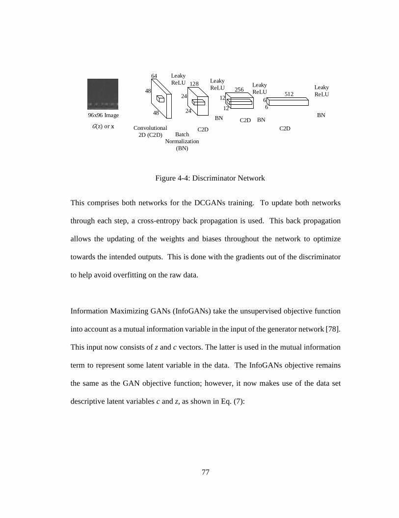
77

Convolutional 2D (C2D)

Leaky ReLU

96x96 Image12

Batch Normalization

(BN)

2448BN BN

C2D

C2DC2D

6

G�z� or x

256128

64

51261224

48

Leaky ReLU Leaky

ReLU

BN

Leaky ReLU

Figure 4-4: Discriminator Network

This comprises both networks for the DCGANs training. To update both networks

through each step, a cross-entropy back propagation is used. This back propagation

allows the updating of the weights and biases throughout the network to optimize

towards the intended outputs. This is done with the gradients out of the discriminator

to help avoid overfitting on the raw data.

Information Maximizing GANs (InfoGANs) take the unsupervised objective function

into account as a mutual information variable in the input of the generator network [78].

This input now consists of z and c vectors. The latter is used in the mutual information

term to represent some latent variable in the data. The InfoGANs objective remains

the same as the GAN objective function; however, it now makes use of the data set

descriptive latent variables c and z, as shown in Eq. (7):

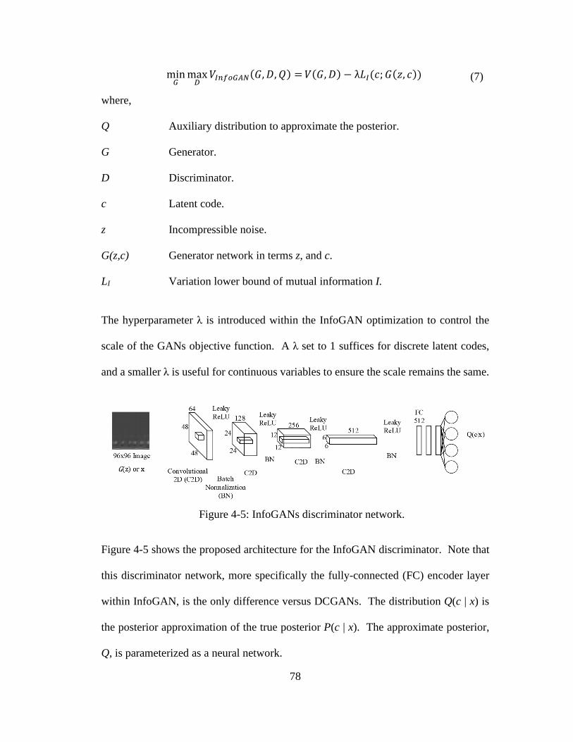
78

minT maxU V�� ¡T¢£�W, X, ¤� = V�W, X� − λ��A; W�§, A�� (7)

where,

Q Auxiliary distribution to approximate the posterior.

G Generator.

D Discriminator.

c Latent code.

z Incompressible noise.

G(z,c) Generator network in terms z, and c.

LI Variation lower bound of mutual information I.

The hyperparameter λ is introduced within the InfoGAN optimization to control the

scale of the GANs objective function. A λ set to 1 suffices for discrete latent codes,

and a smaller λ is useful for continuous variables to ensure the scale remains the same.

Figure 4-5: InfoGANs discriminator network.

Figure 4-5 shows the proposed architecture for the InfoGAN discriminator. Note that

this discriminator network, more specifically the fully-connected (FC) encoder layer

within InfoGAN, is the only difference versus DCGANs. The distribution Q(c | x) is

the posterior approximation of the true posterior P(c | x). The approximate posterior,

Q, is parameterized as a neural network.

79

The benefit to using the InfoGAN algorithm is the ability to extract meaningful features

of the data created by the generator encoder vector. This means, for a fault diagnostic

problem, c encodes the semantic features (fault classes, e.g., baseline, inner race fault,

outer race fault) of the data distribution and z encodes the unstructured noise of the

distribution (e.g., width of the impulse, background noise of the signal). Even with the

mutual information objective function there is no guarantee that the latent variables

found by the trained InfoGAN will be the desired structure in the data. Therefore,

InfoGANs still require visual inspection of the generator images to assess its image

quality. In the following sections, we discuss the steps in the proposed methodology.

4.4.1 Read Raw Signal and Image Representation Construction

Prior to GAN initialization, it is necessary to generate images of the accelerometer data

streaming from the rolling element bearing. Scalogram images contain time and

frequency on the axis and the color depicts the magnitude. Once the images are

generated, the entire data set is subdivided into three groups: training, test, and

validation. It is common to have the bulk of the images in the training set, with the

remainder used as a test set to evaluate the model’s ability to predict the system’s health

classes.

4.4.2 Unsupervised GAN Initialization

Once the scalogram images are generated, Algorithm 3 outlines the process as a means

for a feed forward pipeline for fault diagnosis. Global average pooling is used to reduce

80

the last convolutional layer filters to k vectors of 1x1. This is then concatenated to form

a 1 x k vector and fed into a clustering algorithm.

Algorithm 3 Unsupervised feed forward pipeline for images, i. Train GAN Architecture to data dependent, context dependent epoch count. for i images do • Feed forward pass through the discriminator. • Global Average Pooling for k filters out of last convolutional layer to output k 1x1

filters. • Concatenate last convolutional layer activations (with encoder for the InfoGAN)

from each image i as a 1 x k vector. • Normalize this vector with L2 Norm (Euclidean Distance):

|¨| = © |��|5��(% .

end for • Vector is labeled LA vector for DCGAN. • Vector is labeled LA+encoder vector for InfoGAN. • The resulting vector is fed into a clustering algorithm (k-means++, Spectral) to

obtain labels for images. Once the GAN model is trained (DCGAN or InfoGAN), two additional steps are

needed to evaluate the model. The first step is a visual inspection of the trained

generator network to evaluate the quality of the generated images. Visual inspection of

the output images of the generator network is a key indicator to how well the GAN

architecture is training and whether any of the known drawbacks are surfacing, such as

mode collapse [77], vanishing gradients [78], non-convergence [79], and

checkerboarding artifacts [81]. The second step consists of sampling images from a

random uniform input vector between 0-1. For the InfoGAN, the c input vector is a

random one hot encoded categorical vector. This step uncovers problems in the

convergence of the network, mode collapse to a specific kind of image, or the inability

of the model to generate similar images to the ones in the original dataset.

81

4.4.3 Concatenation, Normalization, and Clustering

To extract the discriminator information after training, a feed forward pass is done with

each image (i) in the dataset to obtain each last convolutional layer activation. These

activations are pooled via global average pooling for each filter (k). This means that,

given k filters in the last layer, the output is k 1 x 1 vectors for each scalogram. After

global average pooling, these vectors are concatenated into a 1 x k vector and

normalized with Euclidean L2 normalization. From this point, the vector output of the

DCGAN is referred to as the last layer activations vector, or LA vector. Moreover, the

output of the InfoGAN includes the encoder output. Therefore, from this point, this

encoder concatenated with the LA vector output of the InfoGAN is referred to as the

LA+encoder vector.

The last step is to use this LA vector or LA+encoder vector (C or Cen, respectively) as

an input into clustering algorithms. For the purposes of this paper, k-means++ and

spectral clustering are examined. Again, this is not a restriction on the methodology; it

is a means to display the robustness of the methodology to two common straightforward

clustering algorithms.

4.4.4 Unsupervised Visual Evaluation – PCA

Once the output of unsupervised clustering is complete, a method to assess the

clustering results without the real labels is needed. For the proposed methodology, one

could evaluate the clustering output of the LA or LA+ vector’s visually to choose the

appropriate number of clusters to proceed with the remainder of the methodology. Note

82

that the GANs training creates a suitable underlying manifold representation of the data

that can be used in a two-dimensional visual inspection. Engineering knowledge can

then be utilized to provide meaning to the evaluation of the visual results of PCA.

4.4.5 Label Data

One of the strengths of the proposed methodology is the ability to feed in an

incrementally increasing amount of labeled data into the training data set of the GANs

algorithm to increase fault class identification results from the clustering. This has

practical importance because, when a new asset comes online, initially there may be

little knowledge of the system faults and their respective raw signals. As more

knowledge is gained, labeled data can be incorporated into the model. The results

section of this paper validates the methodology with metrics for increasing percentages

of labeled data (for validation purposes, it is assumed that labels are known) within the

training data set for semi-supervised fault diagnostics.

4.4.6 Semi-Supervised GAN Initialization

Semi-supervised GAN initialization involves training of the chosen GAN architecture

with an incrementally increasing set of labeled data. This is an important aspect to

explore because as the engineer gains more knowledge about a new system, one can

label small sets of data which are known to be faults to increase the system’s health

state identification via clustering. This approach improves the quality of the clustering

results via a semi-supervised cost function (Eq. 6) as described in Salimans [79]. In the

unsupervised training, the discriminator learns features to avoid classifying the

83

generated data as real data, but these features might not be the best representation given

the implicit labels the problem has. One way to help the discriminator get improved

and more meaningful features for these labels is to use the discriminator as a classifier

for these classes. This is possible with a minor change to the proposed GAN pipeline

outlined in the first step of Algorithm 1. Indeed, the loss function, L, is modified to Eq.

(8), as follows:

� = �ª«¬®¯Fª° + �«�ª«¬®¯Fª° (8)

Where,

�ª«¬®¯Fª° = −Y�,±~¬]^_^��,±� log ��¡°² �v|�, v < G + 1�

�«�ª«¬®¯Fª° = −qY�~¬]^_^�� log `1 − ��¡°² �v = G + 1|��b +Y�~Tlog `��¡°²�v = G + 1|��bt

This cost function adds a cross entropy loss for the first k discriminator outputs. The

unsupervised cost is the same as the original GAN, Eq. (6). However, there is a slight

change as now K+1 corresponds to the probability of the sample being false. The

discriminator is used as a competent classifier given a subset of the dataset. In this case,

the discriminator will be used as a feature extractor given a subset of the dataset to

improve the system’s health state identification results based on clustering. Labels are

used as clues for the structure of the data with the aim of creating an improved

discriminator. This assumes that images generated with semi-supervised learning have

better quality than the ones generated in an unsupervised manner. However, notice that

the main objective of a GAN is to generate data points or images that resemble the

84

training dataset and not to predict any system’s health states. Thus, if we use a few

labeled data points and generated data we are performing a semi-supervised training.

4.4.7 Semi-Supervised Stop Criteria

For a qualitative analysis, the GAN’s last activation layer outputs are used to generate

a two component PCA plot. The ideal result would be a clear separation between the

heath states (classes). If there is not a clear separation, then adding labeled data would

help aid in the separation and provide better system health state diagnosis. It is at this

point the engineer, now with a small number of labels of the fault conditions, can begin

using metrics to evaluate whether the model is performing suitably to cease labeling

additional data. Eventually the quantity of labeled data reaches a point at which the

decision can be made to explore a deep learning enabled fully-supervised fault

diagnostic methodology.

5.0 Examples of Application

In this section, the proposed methodology is applied to both the MFPT and CWR

bearing data sets. To validate the proposed methodology, known labels are available.

Therefore, metrics like purity, NMI, and ARI can be used. GPU computing was

utilized throughout this paper using a system with a Nvidia GPU Titan XP, CPU Core

i7-6700K 4.2 GHz, 32 GB RAM, Tensorflow 1.0, cuDNN 5.1, and Cuda 8.0.

5.1 Machinery Failure Prevention Technology Data Set

This data set was provided by the Machinery Failure Prevention Technology (MFPT)

Society [37]. An experimental test rig with a NICE bearing gathered accelerometer data

85

for three conditions. First, a baseline condition was measured at 270lbs of load and a

sampling rate of 97,656 Hz. Second, ten total outer-raceway faults were

tracked. Three outer race faults were loaded with 270lbs with a sampling rate of 97,656

Hz, and seven outer race faults were assessed at varying loads: 25, 50, 100, 150, 200,

250 and 300 lbs. The sampling rate for the faults was 48,828 Hz. Third, seven inner

race faults were analyzed with varying loads of 0, 50, 100, 150, 200, 250 and 300

lbs. The sampling rate for the inner race faults was 48,848 Hz. Scalogram images, as

shown in Table 4-1, were generated from the raw signal with the following classes:

normal baseline, inner race fault, and outer race fault. The total scalograms images used

for each class was 3,423, 1,981, and 5,404 respectively. With 10,808 total images, the

training set size used was fifty percent. Bilinear interpolation [39] was used to scale the

images down to a manageable size for the training. The MFPT data set is a good test

for any algorithm’s ability to separate the baseline healthy data with the outer race fault

condition. This can be seen in the similarity of the raw signals in Figure 4-6 and Figure

4-8 respectively. Figure 4-7 shows the inner race fault condition.

Figure 4-6: Baseline signal.

Figure 4-7: Inner race fault signal.

86

Figure 4-8: Outer race fault signal.

Table 4-1: 96x96 pixel MFPT scalogram images (actual size).

Baseline Inner Race Outer Race

Within the scalograms of the MFPT data set there are a few areas of notice. The noise

level within the baseline and outer race data appears to be higher than the inner

race. This is confirmed from the plots of the raw signals. The baseline and outer race

faults look similar, hence the potential difficulty in the conducting fault diagnosis on

this data set.

Although labels are available for this dataset, the results presented in this section were

obtained with fully unsupervised training on both DCGAN and InfoGAN architectures,

with complete datasets and without labels. Visual inspection of the output images of

the generator network, as shown in Figure 4-9 and Figure 4-10, is a key indicator to

how well the GAN architecture is training and whether mode collapse, vanishing

gradients, non-convergence, or checkerboarding artifacts is occurring.

87

Checkerboarding artifacts occur when the stride length is not directly divisible by the

convolutional filter size. The output images on this data set show that the generator

performed well in converging to the distribution of the data. It is clear which images

are the inner race fault images, and there is a slight variation in the images generated

for the baseline and outer race conditions.

Figure 4-9: Output images of DCGAN generator training model.

Figure 4-10: Output images of InfoGAN generator training model.

Following the proposed methodology in Section 3 (see Figure 4-2), the alternative

models can be qualitatively evaluated based on the two component PCA. Thus, Figure

88

4-11 shows the PCA results for the best model corresponding to the spectral clustering

based on the InfoGAN LA vector with an output image of 32x32 pixels. Indeed,

Appendix A contains the results for the two component PCA based on both the

InfoGAN and DCGAN data representations. For the sake of brevity, only the results

for the best performing clustering method, spectral clustering, are shown. Both

Appendix A and Figure 4-11 compare the predicted labels with the real labels. Note

that, from the results in Appendix A, the InfoGAN LA vector with an output image of

32x32 pixels provides the best separation and identification of the system’s health

states. This model is closely followed by the InfoGAN LA+ vector with an output

image of 32x32 pixels that, when contrasted to the real labels, shows some difficulty

in separating the baseline health state.

This qualitative evaluation is important within the proposed methodology because for

unsupervised fault diagnostics, the first step for this data representation is a clear

separation between the baseline healthy data and any faulty unhealthy data. The faults

themselves do not necessarily need to be separated from each other at this stage as the

goal of this step is to separate healthy from unhealthy. Isolating faults between each

other can be assessed in a later stage of the proposed methodology as the engineer

begins to label data and has further knowledge into the ground truth of the signals. As

it can be seen from Figure 4-11 for the best model, InfoGAN LA vector with image

output of 32x32 pixels, the baseline is separated well from the rest of the fault signal

data.

89

Real Labels

Predicted Labels

Figure 4-11: Spectral clustering PCA, InfoGAN LA output image 32x32 pixels.

The last convolutional layer activation of the GAN’s generator allows the visualization

of the manifold the GAN developed during training of the underlying gradient basis of

the raw data. This layer holds valuable information about the underlying distribution

of the data.

The effectiveness of the proposed methodology can be evaluated with the following

metrics: Adjusted RAND Index (ARI), Normalized Mutual Information (NMI), and

Purity. ARI and NMI are well known evaluation metrics; however, purity is somewhat

new but used often. Purity, simply put, is the ratio between the dominant class in the

cluster and the size of the cluster. More formally, purity is the following Eq. (9),

Purity�µF� = 1�F max� ��Fo� � ∈ � (9)

where,

w clusters

n members

C number of classes

90

The three metrics used for evaluation all measure different aspects of the effectiveness

of unsupervised learning algorithms. Purity values range from zero (poor clustering)

to one (perfect clustering). A high purity would be easy to achieve if the selected

number of clusters is high. For instance, if every feature from the proposed

methodology had its own cluster, the purity would be one. Therefore, purity cannot be

used to evaluate the number of clusters. NMI allows one to evaluate the tradeoffs of

the number of clusters. However, NMI has the same drawback as purity does where if

there are one-image clusters, NMI has a value of one. The last metric used to evaluate

the clustering output is ARI. ARI, simply put, is the accuracy of the clustering and

measures the percentage of correct decisions. ARI gives equal weight to the false

positives and false negatives. This accounts for the short comings of purity and NMI

where, at times, ARI can perform worse when separating similar data points than

clustering dissimilar data points. From the complete set of results shown in Appendix

B, Tables B.1, B.2, B.3, and B.4, the proposed architectures for the DCGAN and

InfoGAN provide a robust underlying manifold representation of the data and they have

solid performance for unsupervised fault diagnostics. The InfoGAN LA vector with

32x32 output images and with spectral clustering is the one that achieves the best

results: ARI of 0.89, purity equal to 0.96 and NMI of 0.88 as shown in in Table 4-2.

This indicates the proposed methodology is creating pure clusters, the number of

clusters is generating a high NMI, and the ARI accuracy of 0.89 is high for

unsupervised learning.

91

Table 4-2: Fully unsupervised 32x32 generator output, InfoGAN LA output and spectral clustering.

Percent Labeled Data ARI Purity NMI 0% 0.89 0.96 0.88

Moreover, the InfoGAN architecture with the 32x32 generator output outperformed the

96x96 output. This could be explained by the similarities between the baseline and the

outer race fault condition. With increased generator resolution potentially blurring the

images, the GANs models could therefore have a harder time classifying them. Based

on the ARI, NMI, and purity results, there is not a definitive optimal image resolution

for both architectures. Spectral clustering outperformed k-means++ across the

board. The ability of spectral clustering to map to a lower dimensional space allowed

for better predictions. Therefore, for the MFPT data set, the InfoGAN outperformed

the DCGAN. Given the noise the MFPT data set has within two of the classes, the

InfoGAN did a better job of encoding the experimental noise into the z vector.

The next step would be to monitor the system as baseline data is collected. As faults

arise, inspection and knowledge of faults must be completed to ensure the fault

diagnostic system improves. These results indicate a strong value proposition for the

proposed methodology. The proceeding section explores increasing the percentage of

labeled data within this methodology.

As the results of the unsupervised learning are obtained, semi-supervised learning may

be required if some of the results do not meet user requirements for prediction

capability. Even though the fully unsupervised results for this dataset are satisfactory,

92

with best purity scores of 0.96 and 0.82 for the InfoGAN and DCGAN, respectively,

and good separation on the PCA plot for the identification of health states, the semi-

supervised case is explored to see how good the results can be with an investment in

resources to label the data. This is a time consuming and expensive process, so we

analyze different cases that incrementally add labels to the dataset. The percentage of

the labeled data is dependent on knowledge of the failure process, degradation,

application, quality of the data, feeling/expert knowledge, and associated costs. For the

sake of brevity, in this section, we focus on the architecture with the best performance

in the unsupervised stage discussed in the previous section, i.e., the InfoGAN LA vector

with 32x32 generator output. Note also that the models are trained with only a small

portion of the dataset that is labeled.

The top results are reported in Table 4-3 which are for the InfoGAN architecture with

LA output image 32x32 pixels using spectral clustering. To evaluate effectiveness of

the semi-supervised fault identification pipeline, the actual labels are compared to

predicted clusters (predicted health states).

Table 4-3: 32x32 generator output, InfoGAN LA output and spectral clustering.

Percent Labeled Data

Amount of Labeled Data ARI Purity NMI

0% 0 0.89 0.96 0.88 1% 54 0.37 0.73 0.45 2% 108 0.46 0.79 0.59 4% 216 0.82 0.94 0.81 8% 432 0.88 0.96 0.87 10% 541 0.90 0.96 0.88 20% 1,081 0.98 0.99 0.96

Something peculiar in the results is the fact that the metrics performance decreases

initially with the addition of labeled data. This is because the semi-supervised models

93

are trained with labels on a very small portion of the full data set. The most important

part of these validation metric results is the point at which the semi-supervised case

begins outperforming the unsupervised case. This happens at eight percent. The semi-

supervised case is able to match the unsupervised results with only four percent labeled

data and surpass it with eight percent. This gives the engineer a decision point with

which to make an economic decision to start labeling data. Compared to the fully

unsupervised, the semi-supervised results show a better separation overall of the

baseline versus the fault data.

In summary, at a 0.94 purity from the spectral clustering results out of the InfoGAN c

vector, it is worth exploring this unsupervised approach for this dataset before spending

engineering resources on labeling the vast amount of data for similar systems in

industry. Also, with the addition of the labeled data, there are few points worth

commenting. First, spectral clustering still outperformed kmeans++. The results for

the low percentage labeled data show almost equal performance compared with the

unsupervised results, as shown in Appendix B, Tables B.1, B.2, B.3 and B.4. This is

not surprising as the unsupervised results were already high. These results indicate the

unsupervised results can be achieved with a small labeled subset.

5.2 Case Western Reserve University Bearing Data Set

The second experimental data set was provided by Case Western Reserve (CWR)

University Bearing Data Center [6]. A Reliance electric motor, two horsepower, was

used with ball bearings in experiments for the acquisition of vibration accelerometer

94

data on both the drive end and fan end bearings, as shown in Figure 4-12. The signal

is generated from the bearings supporting the motor shaft. Single point artificial faults

were seeded in the bearing with an electro-discharge machining. Location and diameter

of the faults varied for the outer raceway. Additionally, 0 to 3 horsepower motor loads

were included within the experimental data. Accelerometers were attached via magnets

to the housing on the twelve o’clock location.

Figure 4-12: CWR experimental test stand for roller bearing.

For the purposes of this paper four classes were used: baseline, inner raceway, outer

raceway, and rolling element (ball). In total, the images generated for each class was

3,304, IR 2,814, OR 2,819, BF 2,816 respectively. These classes were assembled by

combining the fault sizes, motor speed, and motor load. The training set size again was

set to fifty percent of the 11,753 total images. To ensure the images were a

computationally efficient size, bilinear interpolation [39] was used to scale the images

down to a manageable size for the training. For the CWR data set, any analysis

incorporating the rolling element (ball fault) data requires more sophisticated

algorithms than envelope analysis [41]. Visually, one can see from Figure 4-13, Figure

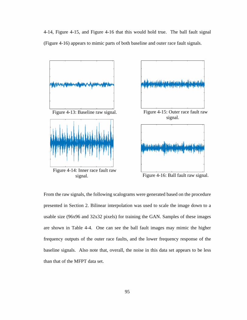
95

4-14, Figure 4-15, and Figure 4-16 that this would hold true. The ball fault signal

(Figure 4-16) appears to mimic parts of both baseline and outer race fault signals.

Figure 4-13: Baseline raw signal.

Figure 4-14: Inner race fault raw

signal.

Figure 4-15: Outer race fault raw

signal.

Figure 4-16: Ball fault raw signal.

From the raw signals, the following scalograms were generated based on the procedure

presented in Section 2. Bilinear interpolation was used to scale the image down to a

usable size (96x96 and 32x32 pixels) for training the GAN. Samples of these images

are shown in Table 4-4. One can see the ball fault images may mimic the higher

frequency outputs of the outer race faults, and the lower frequency response of the

baseline signals. Also note that, overall, the noise in this data set appears to be less

than that of the MFPT data set.

96

Table 4-4: 96x96 pixel CWR scalogram images of the faults. Baseline Inner Race Outer Race Ball Fault

After training both proposed architectures for DCGAN and InfoGAN, the output

images on this data set, as shown in Figure 4-17 and Figure 4-18, appear to show that

the generator performed well in converging to the distribution of the data.

Figure 4-17: Output images of DCGAN generator training model.

97

Figure 4-18: Output images of InfoGAN generator training model.

The PCA of the first two components of the LA vector (DCGAN) and LA+ vector

(DCGAN and InfoGAN) representations are compared. The predicted and real labels

are shown in the Appendix B for all the models based on the best performing clustering

method. For the CWR dataset, this is kmeans++ with the DCGAN LA vector on 96x96

generator images as shown in Figure 4-19. However, one can observe that PCA

operating on the DCGAN and InfoGAN training had difficulties with the baseline data

separation. It appears the ball fault data results in two sets of clusters in the PCA which

is difficult for the clustering methods that do not employ a higher dimensional space to

separate.

Real

Predicted

Figure 4-19: K-means++ PCA, DCGAN LA output image 96x96 pixels.

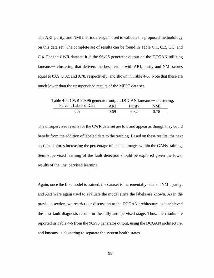
98

The ARI, purity, and NMI metrics are again used to validate the proposed methodology

on this data set. The complete set of results can be found in Table C.1, C.2, C.3, and

C.4. For the CWR dataset, it is the 96x96 generator output on the DCGAN utilizing

kmeans++ clustering that delivers the best results with ARI, purity and NMI scores

equal to 0.69, 0.82, and 0.78, respectively, and shown in Table 4-5. Note that these are

much lower than the unsupervised results of the MFPT data set.

Table 4-5: CWR 96x96 generator output, DCGAN kmeans++ clustering.

Percent Labeled Data ARI Purity NMI 0% 0.69 0.82 0.78

The unsupervised results for the CWR data set are low and appear as though they could

benefit from the addition of labeled data to the training. Based on these results, the next

section explores increasing the percentage of labeled images within the GANs training.

Semi-supervised learning of the fault detection should be explored given the lower

results of the unsupervised learning.

Again, once the first model is trained, the dataset is incrementally labeled. NMI, purity,

and ARI were again used to evaluate the model since the labels are known. As in the

previous section, we restrict our discussion to the DCGAN architecture as it achieved

the best fault diagnosis results in the fully unsupervised stage. Thus, the results are

reported in Table 4-6 from the 96x96 generator output, using the DCGAN architecture,

and kmeans++ clustering to separate the system health states.

99

Table 4-6: CWR 96x96 generator output, DCGAN kmeans++ clustering. Percent

Labeled Data Amount of

Labeled Data ARI Purity NMI 0% 0 0.69 0.82 0.78 1% 117 0.40 0.62 0.42 2% 235 0.47 0.71 0.59 4% 470 0.51 0.69 0.61 8% 940 0.51 0.70 0.55 10% 1,175 0.88 0.95 0.88 20% 2,350 0.95 0.98 0.94

The first evaluation of the results also indicates the same pattern the MFPT results had.

The metric performance decreased as labels were added in smaller quantities. The

point with which the semi-supervised results outperformed the unsupervised results for

this data set is between eight and ten percent. The CWR data set benefited greatly from

the addition of the labels.

Kmeans++ operating on the representation from the DCGAN for this dataset had better

system state separation with labeling a portion of this data set. The purity is much

improved with the top model achieving 0.98 purity with 20% labeled data, whereas the

unsupervised case was only 0.82. The CWR data set is an easily separable data set

using the baseline data, inner race, and outer race faults. With the addition of the ball

fault data, however, one must use more sophisticated methods to perform fault

diagnosis. The CWR data set, in general, has less noise throughout the scalograms than

the MFPT data set. Even without the information from the latent space of the InfoGAN,

the DCGAN architecture provided a better representation for this data, which benefited

greatly from the addition of labeled data.

100

In summary, the CWR predictions performed worse than the MFPT data set predictions

as found in the Appendix C for unsupervised training. Kmeans++ outperformed

spectral clustering but not always. A 32x32 generator output versus a 96x96 generator

output was less clear. For the DCGAN and kmeans++, the 96x96 output performed

better. However, for spectral clustering, both output sizes performed

poorly. Kmeans++ with a DCGAN architecture and a 96x96 pixel generator output

had the highest purity measure.

6.0 Comparison with AE and VAE

To evaluate the proposed methodology, a baseline against AE and VAE was completed

on the same set of scalogram images. The same external clustering evaluation metrics

are used to assess the methodology. The features are extracted from the encoder output

for the autoencoder architecture and from the z-mean output in the VAE case.

For the AE two architectures are considered: one based on fully connected layers

(MLP-AE) and another with convolutional layers (Conv-AE). At least two layers are

used for the encoder / decoder (thus using at least 4 layers given symmetric encoder-

decoder) to allow the AE to generate complex enough features. Given this base

architecture, layers or hidden units are added until the following qualitative criteria is

met: after 10,000 iterations we reconstruct ten images and decide based on image

quality if the decoder generated is a good reconstruction. The loss function is the mean

square error between reconstruction and input image.

101

Based on the procedure established by the proposed methodology, Figure 4-20, Figure

4-21, and Figure 4-22 show the PCA visualizations based on the results obtained from

the MLP-AE, Conv-AE and Conv-VAE architectures, respectively. Note that all PCAs

have an explained variance near 90% so the visualizations are a good approximation of

the general structure of the data.

In the MLP-AE results, the structure of the features is not so clear given the overlap

and the spread of the data structure. An explanation for this behavior is the nature of

MLP when they are used on images: the spatial information is hard to encode, so more

complex transformations are required. This hypothesis is supported comparing this

with the structure found by the Conv-AE where a half moon structure is found. From

the results reported in Table 4-7 (MFPT) and Table 4-8 (CWR), we get consistently

high results in most of the metrics for Conv-VAE. If we consider only purity, the Conv-

VAE is marginally outperformed by MLP-AE for both the MFT and CWR datasets but,

in terms of representation, the Conv-VAE is preferable as shown in Figure 4-22 (MFPT)

and Figure 25 (CWR). The Conv-VAE architecture has the best baseline signal

separation of the three models. Despite these results for the MLP and VAE based

approaches, the proposed GAN based methodology outperforms all models, as it can

be substantiated by comparing the results in Table 4-7 (MFPT) and Table 4-8(CWR)

with Table 4-2 (MFPT) and Table 4-5 (CWR).

102

Table 4-7: MFPT Unsupervised AE and VAE results. Model ARI Purity NMI

MLP AE k-means++ 0.44 0.76 0.49 MLP AE Spectral 0.61 0.82 0.73 Conv AE k-means++ 0.38 0.73 0.49 Conv AE Spectral 0.50 0.81 0.53 Conv VAE k-means++ 0.51 0.81 0.67 Conv VAE Spectral 0.54 0.81 0.69

Figure 4-20: MFPT AE MLP architecture.

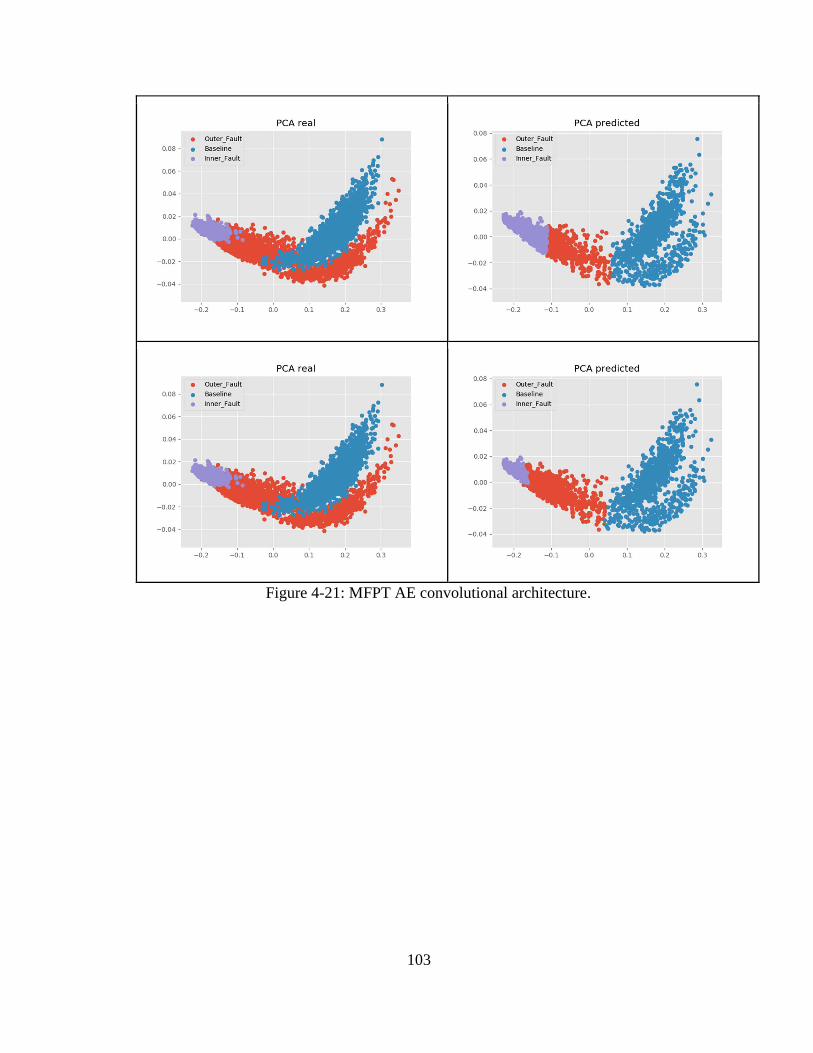
103

Figure 4-21: MFPT AE convolutional architecture.

104

Figure 4-22: MFPT VAE convolutional architecture.

105

Figure 4-23: CWR AE MLP architecture.

106

Figure 4-24: CWR AE convolutional architecture.

107

Figure 4-25: CWR VAE convolutional architecture.

Table 4-8: CWR Unsupervised AE and VAE results.

Model ARI Purity NMI MLP AE k-means++ 0.49 0.69 0.55 MLP AE Spectral 0.35 0.60 0.59 Conv AE k-means++ 0.21 0.53 0.27 Conv AE Spectral 0.38 0.66 0.57 Conv VAE k-means++ 0.50 0.68 0.61 Conv VAE Spectral 0.19 0.55 0.34

These results indicate a limitation of the proposed methodology where the available

clustering evaluation metrics only measure the clustering of a representation, not the

representation itself. However, the representations do exhibit a consistent intrinsic

structure between them. The convolutional VAE and AE together with the GAN

108

representation result in similar structures. The main difference seems to be the ease of

the clustering algorithm to separate this structure. The results indicate that complex

models tend to ease this process with higher ARI, NMI, and purity scores. For example,

in the case of the MFPT dataset, if we compare these results with the top GAN results,

the best non-GAN model ranks fifth best (see Table B.2 and Appendix B). This

indicates that a lower computational cost methodology can achieve reasonable results;

however, to increase ARI, NMI, and purity scores a considerably more complex model

is required.

7.0 Concluding Remarks

Unsupervised fault diagnostics is a critical area of research with applications into many

industries. The ability to detect faults when there is almost zero ground truth, with little

to no labeled data, and from big multi-dimensional machinery data has vast economic

benefits. In this paper, a novel deep generative adversarial multi-stage methodology is

proposed for fault diagnostics. This methodology achieved superior unsupervised

prediction results over both AE’s and VAE’s. These results are then further improved

with the addition of a subset of labeled data.

To achieve the results presented in this paper, the outputs of the activation layers in

both DCGANs and InfoGANs were examined within two traditional clustering

algorithms: 1) k-means++ and 2) spectral. These two clustering algorithms were

chosen to prove the robustness and flexibility of the GAN-based methodology to simple

clustering techniques. The InfoGAN encoder vector was tested as an additional feature

109

for clustering; however, the addition of the encoder information had mixed results. It

appears the InfoGAN architecture outperforms the DCGAN on noisier data like the

MFPT set. Both architectures’ performance benefited from labeling even a small

portion of the data.

While these initial results showed promise, there are limitations and research is in

process to address them. The MFPT data set is simple enough for envelope analysis

classification if the signals are known; however, the CWR data set cannot be diagnosed

with envelope analysis alone. The MFPT data set did include varied loads and multiple

sampling frequencies which were not explored in this work. The amount of data within

each of those data sets was insufficient for the methodology and resulted in overfitting.

Varied rotational speeds were also not explored as the data sets did not contain them.

It is widely known that training a GAN architecture can be challenging. To complete

the work in this study, the training was done multiple times to ensure the GAN

converged towards the Nash equilibrium without mode collapse and vanishing

gradients occurring.

Generative adversarial fault diagnostics paired with the automatic feature learning

inherent with deep learning has great potential benefits for many industries as more

adopt a predictive maintenance program. Generative adversarial networks as a research

topic is still, relatively speaking, in its infancy. It has been accelerating and

proliferating through other research communities at a fast pace since 2014. This is the

first paper to incorporate it into fault diagnostics. The proposed methodology proves

110

that it is flexible enough to incorporate engineering expertise as that expertise grows.

In fact, the proposed methodology demonstrates fault diagnostics are strengthened by

the meaning engineering expertise can give to the learned GAN feature representations.

DCGANs prove their ability to diagnose faults with zero information on the real classes

within the data set. Moreover, InfoGANs show that, with slight knowledge into how

many potential driving failure modes the rolling elements may have, the diagnostics

results may be improved with little economic investment. With integrated

unsupervised and semi-supervised fault diagnostics, industries such as aerospace, wind

power, oil and gas, and automotive are poised to unlock new potentials for diagnostic

and structural health management systems.

111

8.0 Appendix A

Model Predicted Real 32x32

InfoGAN LA

32x32 InfoGAN LA+

32x32

DCGAN LA

112

96x96 InfoGAN LA

96x96

InfoGAN LA+

96x96

DCGAN LA

113

9.0 Appendix B

MFPT Results: 0% (Unsupervised) ARI Purity NMI

LA KMeans++ 0.53 0.80 0.62 LA Spectral Clustering * 0.89* 0.96* 0.88* LA+ KMeans++ 0.57 0.83 0.64 LA+ Spectral Clustering * 0.85 0.95 0.86

Table B. 4-1: 32x32* generator output, InfoGAN.

ARI Purity NMI LA KMeans++ 0.50 0.81 0.58 LA Spectral Clustering * 0.61 0.82 0.72 LA+ KMeans++ 0.42 0.75 0.53 LA+ Spectral Clustering * 0.84 0.94 0.82

Table B. 4-2: 96x96 generator output, InfoGAN.

ARI Purity NMI LA KMeans++ 0.34 0.72 0.47 LA Spectral Clustering * 0.34 0.72 0.48

Table B. 4-3: 32x32 generator output, DCGAN.

ARI Purity NMI LA KMeans++ 0.50 0.79 0.62 LA Spectral Clustering * 0.59 0.82 0.72

Table B. 4-4: 96x96* generator output, DCGAN. * : Indicates best results for clustering. * : Indicates best results for 96x96 or 32x32 output. * : Indicates best results for ARI, Purity, and NMI.

114

10.0 Appendix C

CWR Results: 0% (Unsupervised)

ARI Purity NMI LA KMeans++* 0.565 0.758 0.647 LA Spectral Clustering 0.353 0.604 0.572 LA+ KMeans++* 0.568 0.760 0.647 LA+ Spectral Clustering 0.309 0.640 0.517

Table C. 4-1: CWR 32x32 output, InfoGAN.

ARI Purity NMI LA KMeans++* 0.500 0.766 0.578 LA Spectral Clustering 0.382 0.733 0.510 LA+ KMeans++ 0.463* 0.657 0.495 LA+ Spectral Clustering 0.358 0.715* 0.598*

Table C. 4-2: CWR 96x96 output, InfoGAN.

ARI Purity NMI LA KMeans++* 0.523 0.728 0.579 LA Spectral Clustering 0.347 0.594 0.595

Table C. 4-3: CWR 32x32 output, DCGAN.

ARI Purity NMI LA KMeans++* 0.686* 0.816* 0.781* LA Spectral Clustering 0.241 0.600 0.467

Table C. 4-4: CWR 96x96 output, DCGAN. * : Indicates best results for clustering. * : Indicates best results for ARI, Purity, and NMI.

Acknowledgments

The authors acknowledge the partial financial support of the Chilean National Fund

for Scientific and Technological Development (Fondecyt) under Grant No. 1160494.

115

Chapter 5: A Deep Adversarial Approach Based on Multi-Sensor Fusion for Remaining Useful Life Prognostics4

5.1 Abstract

Multi-sensor systems are proliferating the asset management industry and by proxy,

the structural health management community. Asset managers are beginning to require

a prognostics and health management system to predict and assess maintenance

decisions. These systems handle big machinery data and multi-sensor fusion and

integrate remaining useful life prognostic capabilities. We introduce a deep adversarial

learning approach to damage prognostics. A non-Markovian variational inference-

based model incorporating an adversarial training algorithm framework was developed.

The proposed framework was applied to a public multi-sensor data set of turbofan

engines to demonstrate its ability to predict remaining useful life. We find that using

the deep adversarial based approach results in higher performing remaining useful life

predictions.

5.2 Introduction

Reliability engineering has long been posed with the problem of predicting failures by

using all data available. As modeling techniques have become more sophisticated, so

too have the data sources from which reliability engineers can draw conclusions. The

4 The full-text of this chapter has been published at Verstraete, D. B., et al. " A deep adversarial approach based on multi-sensor fusion for remaining useful life prognostics." 29th European Safety and Reliability Conference (ESREL 2019). Research Publishing Services, 2019. ISBN: 978-981-11-2724-3.

116

Internet of Things (IoT) and cheap sensing technologies have ushered in a new

expansive set of multi-dimensional data which previous reliability engineering

modeling techniques are unequipped to handle.

Diagnosis and prognosis of faults and remaining useful life (RUL) predictions with this

new data are of great economic value as equipment customers are demanding the ability

of the assets to diagnose faults and alert technicians when and where maintenance is

needed [1]. This new stream of data is often too costly and time consuming to justify

labeling all of it. RUL predictions, being the most difficult, are also of the most value

for the asset owner. They provide information for a state-of-the-art maintenance plan

which reduces unscheduled maintenance costs by avoiding downtime and safety issues.

Therefore, taking advantage of unsupervised learning-based methodologies would

have the greatest economic benefit. Deep learning has emerged as a strong technique

without the need for previous knowledge of relevant features on a labeled data set [1].

If faulty system states are unavailable or a small percentage of the fault data is labeled,

deep generative modeling techniques have shown the ability to extract the underlying

two-dimensional manifold capable of diagnosing faults.

Deep learning has been employed with success to remaining useful life estimation

(RUL). [54] employed a recurrent neural network (RNN) for RUL estimation. [55],

[56], [57], [58], [59], [60], and [61] all employ long short-term memory (LSTM)

networks to estimate RUL. [62] incorporates feature extraction coupled with a deep

117

neural network for RUL estimation. [63] uses convolutional neural networks (CNN)

and time-windowing to estimate RUL.

These previous works into RUL estimation do not attempt to develop an understanding

of the underlying generative or inference model. Moreover, they used datasets which

were fully labeled. Generative modeling provides the possibility to accomplish this

without having to label what could be massive multi-dimensional noisy sensor data.

Labeling this data would be costly and difficult. A valuable methodology would

provide the flexibility to include a small percentage of labeled data as it becomes

available.

To address these problems, this paper proposes the first algorithm which incorporates

both variational and adversarial training for RUL prognostics. The novelty of this

method has vast applications for fault diagnosis and prognosis. Furthermore, it can be

incorporated for both new and existing system assets.

5.3 Background

5.3.1 Generative Adversarial Networks

Generative Adversarial networks (GANs) are a class of generative models where the

density is learned implicitly via minimax game [47]. This game’s objective is to learn

a generator distribution ¶T�� identical to the real data distribution ¶°·D·��. When

one does not necessarily want to explicitly obtain an inference model to diagnose a

118

system fault and assign probability to every data � in the distribution, GANs are a

viable alternative. To accomplish this, the generator trains a neural network (NN)

capable of generating the distribution ¶T�� by transforming a vector of random noise

variables, ¶�¡Fª�z�. The generator’s objective, W�z�, is trained by playing against an

adversarial discriminator network parameterized by a separate neural network whose

objective, X�x�, is to classify the data as real or fake. The optimal discriminator

X�� = ¶°·D·�x� `¶°·D·�x� + ¶T��b⁄ would ideally converge to the Nash Equilibrium

[64]; however, there is no mechanism to control this. Formally, this value function is

Eq. (10):

minT max U V�W, X�= YZ~\]^_^�Z�`log �X�x�b+ Yc~\defgh�c�`log �1 − X�W�z��b.

(10)

where, Pdata(x) is the data distribution, Pnoise(x) is the noise distribution, D(x) is the

Discriminator objective function, and G(z) is the generator objective function.

5.3.2 Variational Autoencoders

Variational autoencoders (VAEs) are a class of explicit generative models which yields

both inference and generative models [66]. VAEs attempt to learn a model, ��|§�, of

latent variables, §, which generates the observed data, �. Commonly ��|§� ≡�¹��|§� is parameterized by a neural network with parameters º. For most cases the

posterior distribution ��§|�� is intractable. However, an approximate posterior

119

distribution, »¼�§|��, can be used to maximize the evidence lower bound (ELBO) on

the marginal data log-likelihood. Formally, this is expressed as Eq. (11),

log��x� ≥ Y½¾�§|��`log�¹��|§�b − KL�»¼�§|��||��§�� (11)

From this, the objective is equivalent to minimizing the Kullbeck-Liebler (KL)

divergence between »¼�§|�� and ��§|��. Note that »¼�§|�� is usually parameterized

by a neural network with parameters À. VAEs have been successfully applied to fault

diagnosis problems in the recent past [65].

5.4 Proposed Framework

In this work, we propose a mathematical framework that encapsulates the following

features: non-Markovian transitions for state space modeling (i.e., it is not assumed that

all information regarding past observation is contained within the last system state),

adversarial training mechanism on the training of the recognition »¼�§D|§%:D$%, �%:D�, variational Bayes for the inference and predictive model �¹��D|�%:D$%, §%:D�, and

adversarial variational filtering algorithm. We set �D as the observed sensor data, §D as

the latent system state, ÀD is the recognition model parameters, ºD is the inference

model parameters, and vD is the target domain relevant to the adversarial training v ∈0,1, … , ��.

We denote the latent sequence zD ∈ Â ⊂ ℝ�Ä as a set of real numbers �Å. We denote

observations xD ∈ Æ ⊂ ℝ�� dependent on inputs uD ∈ � ⊂ ℝ�Ç. Where Æ is

potentially, but not limited to, a multi-dimensional data set consisting of multiple

sensors from a physical asset. The observations themselves are not constrained to a

120

Markovian transition assumption. Therefore, these transitions can be complex non-

Markovian. This is often the case for engineering problems like crack growth and

environmental effects on RUL. We are interested in the probabilistic function sequence

��D|§%:D$%� generated by the discrete sequences �D = ��%, �5, … , �D� and §%:D$% =�§%, §5, … , §D$%�, as shown in Eq. (12).

��D|�%:D$%� = 7 ��D|�%:D$%, §%:D��§%:D|§%:D$%�>§%:D (12)

z%:D$%, zD ∈ Â ⊂ ℝ�Ä denotes the latent sequence. The underlying latent dynamical

system is assumed to have a generative model basis with emission model

��D|�%:D$%, §%:D� and transition model ��§D|§%:D$%�. Two assumptions, Eq.’s (13) and

(14) are classically imposed on emission and transition models to obtain the state space

model,

��D|�%:D$%, §%:D� = È ��D|§D�DF(% (13)

��§D|§%:D$%� = È ��§D9%|§D�D$%F(É (14)

It is assumed that the current state §D contains complete information for both the

observations �D, and the next state §D9%. These assumptions are insufficient for

complex non-Markovian transitions on noisy multi-dimensional sensor data.

Therefore, we propose the objective function as shown in Eq. (15) which gives us an

expressive approximate inference model »¼�§D|�D�. The mathematical formulation

characterizes the state space model without assumptions as outlined in Eq.’s (11) and

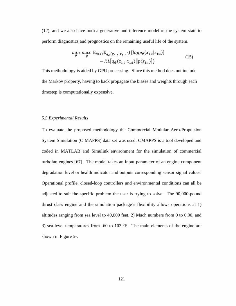
121

(12), and we also have both a generative and inference model of the system state to

perform diagnostics and prognostics on the remaining useful life of the system.

Ê��¹ Ê3� ¼ YU��Y½¾�§%:DË�%:D ��`��Ì�¹��%:D|§%:D�b− G�Í»¼�§%:D|�%:D�Î��§%:D�Ï�

(15)

This methodology is aided by GPU processing. Since this method does not include

the Markov property, having to back propagate the biases and weights through each

timestep is computationally expensive.

5.5 Experimental Results

To evaluate the proposed methodology the Commercial Modular Aero-Propulsion

System Simulation (C-MAPPS) data set was used. CMAPPS is a tool developed and

coded in MATLAB and Simulink environment for the simulation of commercial

turbofan engines [67]. The model takes an input parameter of an engine component

degradation level or health indicator and outputs corresponding sensor signal values.

Operational profile, closed-loop controllers and environmental conditions can all be

adjusted to suit the specific problem the user is trying to solve. The 90,000-pound

thrust class engine and the simulation package’s flexibility allows operations at 1)

altitudes ranging from sea level to 40,000 feet, 2) Mach numbers from 0 to 0.90, and

3) sea-level temperatures from -60 to 103 oF. The main elements of the engine are

shown in Figure 5-.

122

Figure 5-1: Simplified diagram of engine simulated in C-MAPPS [67].

Specifically, for this paper, FD001 of the PHM 2008 competition data set using

CMAPPS is used for this analysis and application.

Figure 5-2: FD001 RMSE results vs training step for 50 iterations with the lowest result (14.69) marked.

The results from training fifty iterations and RUL estimations are a mean of 16.91

RMSE and a standard deviation of 1.48. The lowest result from the training was an

RMSE of 14.69 as shown in Figure 5-2. These results are very good and near the state-

of-the-art results for this data set. The output of the framework also includes a

generative model that gives the engineer the ability to potentially generate more data.

Moreover, these results are fully unsupervised learning, whereas similar results are

fully supervised estimations [69]. Further research will address these gaps and refine

the results on a real-world application.

14.690

20

40

60

80

100

0 200 400 600 800 1,000

Ro

ot M

ean

Sq

uar

e E

rro

r

123

5.6 Conclusions

In this paper we have proposed a deep learning enabled adversarial-variational

mathematical framework for remaining useful life estimation. Unsupervised RUL

estimation is a critical area of structural health monitoring research. It has many

applications into numerous industries. This mathematical formulation is the first

application of its kind and shows great promise.

The proposed mathematical framework demonstrates a solid ability to predict the

remaining useful life of the asset. An engineer can decide whether to plan for

maintenance before a failure occurs and make the necessary arrangements. The

application of the mathematical framework is not only limited to turbo-fan engines.

Oil and gas, wind turbine farms, automotive, and aero-space can all benefit from this

research.

Acknowledgements



124

Chapter 6: A Deep Adversarial Approach Based on Multi-Sensor Fusion for Semi-Supervised Remaining Useful Life Prognostics5

6.1 Abstract

Multi-sensor systems are proliferating in the asset management industry. Industry 4.0,

combined with the Internet of Things, has ushered in the requirements of prognostics

and health management systems to predict the system’s reliability and assess

maintenance decisions. State of the art systems now generate big machinery data and

require multi-sensor fusion for integrated remaining useful life prognostic capabilities.

To address this challenge, this paper proposes a deep adversarial approach to remaining

useful life prediction in which a non-Markovian variational inference-based model

incorporating an adversarial methodology is developed. The evaluate the proposed

approach a public multi-sensor data set for turbofan engines is used for remaining

useful life prediction. The proposed approach is then compared against similar deep

learning models.

6.2 Introduction

Reliability is defined as the ability of a product or system to perform its required

functions without failure for a specified time and when used under specified conditions.

Therefore, reliability engineering has long been tasked with predicting the remaining

useful life of systems by incorporating all available data. Reliability engineering has

5 This chapter has been published at Verstraete, D.; Droguett, E.; Modarres, M. A Deep Adversarial Approach Based on Multi-Sensor Fusion for Semi-Supervised Remaining Useful Life Prognostics. Sensors 2020, 20, 176.

125

been given technologies incorporating cheap sensing with the Internet of Things (IoT)

generating multi-dimensional data sets through Industry 4.0 [1]. With this new data at

the engineer’s fingertips, more sophisticated methodologies to handle this data have

been developed and expanded the prognostics and health management (PHM) field.

These data sets are often costly and time-consuming to label [2]. The engineer therefore

must make an economic decision on how much data to label. Therefore, the greatest

economic benefit would be to take advantage of unsupervised learning-based

methodologies. To understand relevant system health states without labeling, deep

learning methodologies have been shown to be a technique employed without the need

for previous knowledge of degradation processes [65].

Most recently, remaining useful life (RUL) research focused on fully supervised deep

learning methodologies has had success RUL prediction [69]-[85]. These models

depend on the analyst having access to a fully labeled dataset. Therefore, these RUL

prediction accuracies require the use of accurate training data labels. Moreover, this

previous research does not attempt to develop the underlying generative or inference

model. A reliability engineer does not always have the resources to label all the data

necessary to train a deep learning model. A valuable methodology would provide the

flexibility to include a small percentage of labeled data as it becomes available and

resources allow. Generative modeling is a class of modeling techniques which provides

the ability to predict RUL without having to label what could be massive multi-

dimensional sensor data.

126

There have been recent efforts in generative modeling research, although it has yet to

be adapted and applied to reliability and machine health prognostics. Indeed, [86] and

[87] both employed the variational autoencoder (VAE) principles to times series

observations. [88] encodes the state space assumptions from within their proposed

structure inference deep Kalman filter-based methodology. [89] proposes a VAE

principled state-space filtering methodology in which the latent space is forced to fit

the transition. [90] present VAEs based on adversarial training, and they achieve the

flexibility to represent families of conditional distributions over latent variables. [91]

combine GANs with VAE by proposing a new interpretation of adversarial domain

adaptation (ADA) and a unifying generative modeling framework named through

comparisons with the wake sleep algorithm [92]. These methods, while suited for their

applications in computer science, lack the requirements for RUL predictions, such as

time series applications. The Markovian assumption is also utilized, where it is

assumed that all information of past observations is contained within the last system

state; however, for prognostics and health management (PHM), this is insufficient.

Multiple operating conditions increase the degradation complexity of the RUL

predictions, and some degradation paths are inherently non-Markovian (e.g., crack

growth). VAE on their struggle with low probability events, like curb strike events

inherent in large systems [36]. Additionally, for PHM applications with unsupervised

RUL, these methods lack the VAE combined with the adversarial training of a GAN

on time-series data to provide predictions.

127

To address these problems, this paper proposes a deep generative state-space modeling

methodology for the remaining useful life prognostics of physical assets. The

mathematical framework underpinning the proposed methodology delivers the

following novel contributions for RUL predictions: (i) Non-Markovian transitions from

multi-dimensional sensor data by generalizing a deep generative filtering approach for

remaining useful life estimation of the system; (ii) a modeling approach that

incorporates both variational and adversarial mechanisms; (iii) flexibility to handle

both unsupervised and semi-supervised learning for the estimation of the remaining

useful life. This method has vast applications for RUL predictions on both new and

existing system assets.

The rest of the paper is organized as follows. Section 2 provides a brief overview of

GAN, VAE, and state-space modeling. Section 3 presents the proposed methodology

and the underlying mathematical framework. Section 4 overviews the experimental

results. Section 5 concludes with discussions and future work.

6.3 Background

The generative modeling research as mentioned above, [86-92], all aim to tackle

the problem of both a generative manifold space and inference modeling for prediction.

There are slight differences between generative and inference modeling, but

fundamentally they aim to solve the same problem: black-box neural transformations

for implicit distribution modeling between the latent and visible spaces. For RUL

estimation, reliability and PHM, this is equivalent to modeling the underlying

degradation space, z, that is a result of the acquired observed sensor data set, x.

128

Generation Model

Inference Model

x x

z zPrior Distribution

Data Distributionz ~ pdata�z�

x ~ pdata�x�

x ~ f’black-box�z�

z ~ f’black-box�x�

Figure 6-3: Generative and inference modeling similarities (Adapted from [91]).

Traditional generative modeling approaches tend to distinguish between latent and

visible variables clearly and treat them differently. However, a key aspect in generative

modeling is that a clear boundary between the latent and visible variables (as well as

generation and inference) is not necessary. Instead, viewing generative modeling as a

symmetric pair helps in modeling and understanding as shown in Figure 6-3.

6.3.1 Generative Adversarial Networks

Generative Adversarial Networks (GANs) are a class of generative modeling

techniques where two neural networks compete via a minimax game [64]. This game’s

objective is to develop/learn a generator distribution ¶T�� able to generate fake data

identical to the real data distribution ¶°·D·��. However, the generator does not

directly have access to the real data. Instead, the generator distribution, ¶T��,

transforms a vector of random noise, ¶Å�z�, with objective function, W�z�. The

generator is then trained against an adversarial discriminator network parameterized by

a separate neural network whose objective, X�x�, is to classify the data as real or fake,

as shown in Figure 6-4.

129

Real Data

Fake Dataz~pz(z)

x~pdata(x)

GeneratorG(z)

DiscriminatorD(x)

Figure 6-4: Generative Adversarial Networks

There is no mechanism within the GAN training to constrain and control the Nash

Equilibrium point; however, the optimal discriminator X�� =¶°·D·�x� `¶°·D·�x� + ¶T��b⁄ should converge to equilibrium [64]. Formally, this

value function is shown in Eq. (16):

minT max U V�W, X�= YZ~\]^_^�Z�`log �X�x�b+ Yc~\defgh�c�`log �1 − X�W�z��b.

(16)

where, G(z) is the generator objective function, D(x) is the discriminator objective

function, Pdata(x) is the data distribution, and Pz(x) is the noise distribution.

6.3.2 Variational Autoencoders

Variational autoencoders (VAEs) are a class of generative models which develops both

an inference and a generative model [66]. VAEs attempt to develop a model of latent

variables, §, which can generate the observed data, �. Formally, this is expressed as:

130

�� = 7 ��, §�>§ = 7 ��|§��§�>§ (17)

It is common for ��|§� ≡ �¹��|§� to be developed and parameterized by a neural

network with parameters º. For most cases, the posterior distribution ��§|�� is

intractable. However, an approximate posterior distribution, »¼�§|��, can be used to

maximize the evidence lower bound (ELBO) on the marginal data log-likelihood:

log��x� ≥ Y½¾�§|��`log�¹��|§�b − KL�»¼�§Ë��|Ë��§��b (18)

From this, the objective is equivalent to minimizing the Kullback-Liebler (KL)

divergence between »¼�§|�� and �¹��|§�. Note that �¹��|§� and »¼�§|�� are usually

parameterized by two neural networks with parameters À and θ as shown in Figure 6-

5.

Encoder Decoder

Input

Hidden

Outputqϕ �z|x� pθ �x|z�

Figure 6-5: Variational autoencoder

The training of a VAE involves the training of two neural networks, the encoder,

»¼�§|�� sometimes referred to as the recognition model, and the decoder, �¹�§|��

sometimes referred to as the generative model. The encoder learns the relevant features

131

of the input data and compresses the information to the latent hidden space. The

decoder then attempts to generate signals (e.g., images) identical to the input data and

the reconstruction error is then minimized.

Within the computer vision community, VAEs tend to produce blurred images that are

not as sharp as those produced by other generative models. Within an engineering

context, VAEs on their own can result in a common issue with particle filtering

algorithms: without a fully expressive generative model capable of handling extremely

low probability events or sensor reading interactions, the resulting prognosis model

may not have considered these non-Markovian events.

6.4 Proposed Methodology

Given the complexities and associated uncertainty of the fault diagnostic and

prognostic problem, a proposed methodology would be one that is flexible enough to

include new sets of information as they become available. Expert opinion, black swan

events, abnormal operating conditions, knowledge of the underlying failure modes,

physics of failure models, and partially relevant information can all be included within

the remaining useful life estimation. While this information can be valuable, the

methodology should also adequately generalize this data. For example, extracting

relevant features, which may be known, may not be able to account for noisy sensor

signals or operating conditions outside the norm. With this end, we propose the

methodology shown in Figure 6-6.

132

Unsupervised Feature Learning

Adversarial-Variational Model

Continued RMSE Improvement

Raw Signal Start

End

Semi-Supervised RUL Prediction Semi-Supervised RUL Prediction

No

No

Continued RMSE Improvement

Estimate RMSE

Yes. Increase % Labels

Proceed to Semi-Supervised Feature Learning?

Semi-supervised Feature Learning

Adversarial-Variational Model

Estimate RMSE

Yes

No

Yes. Increase % Labels

Figure 6-6: Proposed deep generative methodology for remaining useful life estimation.

The methodology has two distinct phases: 1) Unsupervised learning assessment of

RUL, 2) Semi-supervised learning assessment of RUL. It starts with the raw data signal

fed into the unsupervised variational adversarial filter. Without knowledge of labeling

(e.g., the system health states) at the start of operation of the system, this stage of

development requires the use of unsupervised remaining useful life estimation. Once

the system has had operational time, the engineer is able to start labeling data in a semi-

supervised iterative loop, i.e., identify the system’s health states with corresponding

input sensor data patterns. As it may not be feasible (time and cost wise) to do so for

all the available data, experiments have shown that semi-supervised methodologies

with only a few percentages of the data set labeled can substantially improve the

133

unsupervised methods [65]. Therefore, as the engineer labels data, the framework is

robust enough to handle this percentage of labeled data, as it shall be demonstrated later

in Section 6.5.

6.4.1 Unsupervised Remaining Useful Life Formulation

In this work, we propose a mathematical formulation that encapsulates the following

features: both unsupervised and semi-supervised feature learning, adversarial-

variational state-space modeling with non-Markovian transitions (i.e., it is not assumed

that all information regarding past observation is contained within the last system state),

adversarial training mechanism on the training of the recognition »¼�§D|�%:D�, and

variational Bayes for the inference and generative model �¹��D|§%:D�. As shown in

Figure 6-7 and Figure 6-8, where we set �D as the observed sensor data, §D as the latent

system health state (e.g., crack length, degradation), and vD is the target domain relevant

to the adversarial training v ∈ 0,1, … , ��. Blue lines represent adversarial

mechanism, dashed lines indicate inference processes, and solid lines indicate a

generative process. The transition parameters, ºD, are inferred via a neural network.

Past observations are directly included in the inferential model output. The proposed

mathematical framework does not assume that all the information relevant to ÀD is

encoded within §D.

134

θt

Remaining Useful Life

zt+1 zt+2 ztn

Prognostic

yt+1 yt+2 ytn...

...

xt yt

...

Current State

z1 z2 zt-1 zt

DiagnosticFuture State

Figure 6-7: Forward graphical model for the proposed mathematical framework.

ϕ t

xt+1

...z1 z2 zT zt

Figure 6-8: Inference training model.

To establish the training optimization, we denote the latent sequence zD ∈ Â ⊂ ℝ�Ä as

a set of real numbers �Å and observations as xD ∈ Æ ⊂ ℝ��. Æ can be, but is not limited

to, a multi-dimensional sensor data set from a large asset. The observations, xD, are not

constrained to a Markovian transition assumption. For engineering problems (eg.,

crack growth and environmental effects on RUL) these transitions can be complex non-

Markovian. Therefore, the degradation sequence ��D|§%:D$%� generated by the discrete

135

multi-dimensional sensor data sequences �D = ��%, �5, … , �D� and §%:D$% =�§%, §5, … , §D$%� are of interest to the engineer, as shown in Eq. (19):

��D|�%:D$%� = 7 ��D|�%:D$%, §%:D��§%:D|§%:D$%�>§%:D (19)

where, z%:D$%, zD ∈ Â ⊂ ℝ�Ä denotes the latent sequence. The basis of the latent

dynamical system is assumed to have an emission model ��D|�%:D$%, §%:D� and

transition model ��§D|§%:D$%�. Two assumptions are classically imposed on the

emission and transition models models as shown in Eq.’s (13) and (14),

��D|�%:D$%, §%:D� = È ��D|§D�DF(% (20)

��§D|§%:D$%� = È ��§D9%|§D�D$%F(É (21)

These equations capture the assumption that the current state, §D, holds complete

information for the observations �D, and the subsequent state §D9%. For noisy multi-

dimensional sensor data sets with complex non-Markovian transition this assumption

is insufficient. The proposed mathematical formulation characterizes the state-space

model without these assumptions.

Therefore, to derive the proposed mathematical framework of the proposed

methodology, we first put forward the variational lower bound objective function from

Eq. (19) given that we do not make the Markov assumption from Eq. (20) and (21).

Thus, we have:

136

G� *»¼�§%:D|�%:D �||��§%:D|�%:D �/ = − 7 »¼�§%:D|�%:D � ×��Ì Ø ��§%:D|�%:D �»¼�§%:D|�%:D �ÙÚ (22)

As we know that,

��§%:D|�%:D� = ��%:D, §%:D��%:D� (23)

= − 7 »¼�§%:D|�%:D� Û��Ì Ü ��%:D, §%:D��%:D�»¼�§%:D|�%:D�ÝÞ (24)

= − 7 »¼�§%:D|�%:D� ×��Ì Ø ��%:D, §%:D�»¼�§%:D|�%:D� ∗ 1��%:D�ÙÚ (25)

= − 7 »¼�§%:D|�%:D� ×��Ì ��%:D, §%:D�»¼�§%:D|�%:D� + ��Ì 1��%:D�Ú (26)

= − 7 »¼�§%:D|�%:D� ×log ��%:D, §%:D�»¼�§%:D|�%:D� − log ��%:D�Ú (27)

= − 7 »¼�§%:D|�%:D� ×��Ì ��%:D, §%:D�»¼�§%:D|�%:D�Ú+ 7 »¼�§%:D|�%:D�Å ��Ì ��%:D� (28)

However,

��Ì ��%:D� 7 »¼�§%:D|�%:D�Å = 1 (29)

Therefore, we have,

137

��Ì��%:D�= G�Í»¼�§%:D|�%:D �||��§%:D|�%:D�Ï + 7 »¼�§%:D|�%:D� ×��Ì ��%:D, §%:D�»¼�§%:D|�%:D �Ú (30)

where we simultaneously want to minimize the Kullback-Liebler (KL) divergence and

maximize the variational (evidence) lower bound (ELBO), ℒ�º, À; �%:D�, as shown in

Equation (31):

ℒ�º, À; �%:D� = 7 »¼�§%:D|�%:D � ×��Ì ��%:D, §%:D�»¼�§%:D|�%:D�Ú (31)

Now, rearranging Equation (31), we have the non-Markovian variational lower bound

derived for time series data in Equation (32):

ℒ�º, À; �%:D� = Y½¾�§%:DË�%:D �`��Ì�¹��%:D |§%:D�b− G�Í»¼�§%:D|�%:D�Î��§%:D�Ï (32)

To add in adversarial training, we follow [47] and we rewrite the optimization function

from Equation (32) to Equation (33) as follows:

Ê��¹ Ê3� ¼ YU��Y½¾�§%:DË�%:D ��`��Ì�¹��%:D|§%:D�b− G�Í»¼�§%:D|�%:D�Î��§%:D�Ï�

(33)

We now have an objective function which gives us an expressive »¼�§D|�D, §%:D$%�, that

is, we have a mathematical framework the characterizes the state space model without

the restrictive assumptions outlined in Equations (20) and (21). Additionally, this

mathematical framework contains both a generative and inference models of the system

138

state that allows us to perform fault diagnostics and prognostics as well as remaining

useful life of the system assessment.

6.4.2 Semi-Supervised Loss Function

Semi-supervised initialization involves training of the chosen model’s architecture with

an incrementally increasing set of labeled data. This is an important aspect to explore

because as the engineer gains more knowledge about a new system, one can label small

sets of data which are known to be system degradation versus healthy operation to

increase the system’s health state prediction. This approach can improve the quality of

the results via a semi-supervised cost function given as given by Eq. (34):

� = �ª«¬®¯Fª° + �«�ª«¬®¯Fª° (34)

In the context of the proposed adversarial framework, during the unsupervised training,

the discriminator learns features to avoid classifying the generated data as real data, but

these features might not be the best representation. To improve the discriminator and

develop more meaningful features for the system’s health states over time, labels are

used. This is possible by writing the loss function, L, within training to some

predetermined number of epochs as follows:

�ª«¬®¯Fª° = −Y�M:_,±M:_~¬]^_^��M:_,±M:_� log ��¡°² �v%:D|�%:D , v%:D < G + 1� (35)

�«�ª«¬®¯Fª° = −qY�~¬]^_^��M:_� log `1 − ��¡°² �v%:D

= G + 1|�%:D�b + Y�~Tlog `��¡°²�v%:D = G + 1|�%:D�bt (36)

This cost function adds a cross-entropy loss for the first K discriminator outputs. The

unsupervised cost is the same as the original GAN (see Eq. (16)(10)). However, there

is a slight change as now K+1 corresponds to the probability of the sample being false

139

[79]. The discriminator is used as a competent classifier given a subset of the dataset.

In the context of the proposed mathematical framework, the discriminator will be used

as a feature extractor given a subset of the dataset to improve the system’s health state

identification results.

6.5 Experimental Results

To evaluate the proposed methodology, the Commercial Modular Aero-Propulsion

System Simulation (C-MAPSS) data set was used. CMAPSS is a tool developed and

coded in MATLAB and Simulink environment for the simulation of commercial

turbofan engines [67]. The model takes an input parameter of an engine component

degradation level or health indicator and outputs corresponding sensor signal values.

Operational profile, closed-loop controllers and environmental conditions can all be

adjusted to suit the specific problem the user is trying to solve. The 90,000-pound

thrust class engine and the simulation package’s flexibility allows operations at 1)

altitudes ranging from sea level to 40,000 feet, 2) Mach numbers from 0 to 0.90, and

3) sea-level temperatures from -60 to 103 oF. The main elements of the engine are

shown in Figure 6-9.

140

Figure 6-9: Simplified diagram of engine simulated in C-MAPSS [67].

Specifically, for this paper, the PHM 2008 competition data set using CMAPSS is used

for this analysis and application [67]. Four data sets, FD001 through FD004 are

available and have the properties shown in Table 6-.

Table 6-1: CMAPSS Data Overview Data Set Train

Trajectories Test

Trajectories Conditions Fault Modes

FD001 100 100 1 (Sea Level) 1 (HPC) FD002 260 259 6 1 (HPC) FD003 100 100 1 (Sea Level) 2 (HPC, and Fan) FD004 248 249 6 2 (HPC, and Fan)

The four data sets have a combination of two fault conditions: high pressure compressor

(HPC) degradation and fan degradation. The data set is separated into training and test

sets consisting of 26 sensor measurements, three conditions of operation, engine

quantities, and the cycle time. Each of the engines within the dataset initiate with

different levels of manufacturing variation and initial degradation. This information is

hidden from the engineer and is not considered a fault condition. The three operational

settings do have a substantial effect on the engine performance. These settings are

known. Finally, the sensor data is contaminated with noise. To avoid unnecessary

repetitions, the following sections use FD001 and FD004 for the sake brevity.

141

6.5.1 CMAPSS Results

To evaluate the proposed semi-supervised methodology, two types of labeling were

used: 1) fixed interval and 2) random interval. The fixed interval consists of labeling

one out of every x number of labels, (i.e., 5% equals labeling 1 out of every 20 data

points.) Random interval labeling consisted of taking a random sample of the complete

data set for labeling (i.e., 5% of 15,680 data points equals 784 randomly labeled data

points). This was done because, as the time interval between labels is decreasing, the

RUL estimation error improvements reduce. As one will notice in the rest of this

section, this did have an effect on RUL prognostics.

To evaluate the effects of adding a small subset of labeled data to the training

procedure, semi-supervised learning was also conducted on the CMAPSS dataset.

There are two parts of the algorithm to evaluate this effect of labeling on the results:

1) feature learning and 2) regression. When it is stated “semi-supervised feature

learning” it implies that percentage of labels were fed into the feature learning phase

of the model. When results are reported as “unsupervised feature learning”, zero labels

were used in the feature learning portion of the model.

The proposed methodology is evaluated against the true RUL via root mean square

error (RMSE). To not sway these results in a more positive light, the authors chose to

train the model ten times and take the average results from all ten.

142

First FD001 is evaluated from one percent to one hundred percent labels. The RMSE

results can be found in Table 6-2 and Table 6-3. As one can see from the results, there

is an effect on the RUL prognostics with both types of labeling (fixed vs random) and

adding labels to both parts of the model. This can also be viewed in Figure 6-10. There

are two observations to note when looking at the results: 1) adding labels to feature

learning improves the RUL prediction, and 2) as more labels are added to the feature

learning and regression parts of the modeling the prediction performance (in terms of

RMSE) improvement tends to taper off after twenty percent. The increase in prediction

performance from adding labels to the feature learning portion of the model shows that

feeding labels to the generative model help extract more degradation related features

present in the data. The appropriate percentage of labeling could be inferred or

determined based on the evolution of the RMSE according to Figure 6-10. In this case,

the RMSE marginally improves for FD001 beyond twenty percent labeling (1.5%

improvement for 50% labeling and 2.7% improvement for 100% labeling). This is

important because labeling data is expensive and time consuming. Therefore,

increasing the prediction performance (i.e., reducing RMSE) beyond twenty percent

labels becomes increasingly more expensive for a smaller benefit.

Table 6-2: FD001 RMSE Unsupervised feature learning with semi-supervised regression

Labeling 1% 5% 10% 20% 50% 100%

Fixed 23.33 19.34 18.26 17.66 17.39 16.91 Random 24.54 19.66 19.17 18.50 17.96 17.57

143

Table 6-3: FD001 RMSE Semi-supervised feature learning with semi-supervised regression

Labeling 1% 5% 10% 20% 50% 100%

Fixed 20.50 18.50 17.47 16.37 15.82 15.44 Random 21.20 18.33 16.50 16.06 15.54 15.27

Figure 6-10: FD001 RMSE versus percent labeled (%).

To evaluate the effects and differences of modeling operating conditions and additional

fault modes, FD004 was also examined. This data set is more applicable for cases that

include fleets of vehicles operating in different conditions. Base on the results reported

in Figure 6-11, Table 6-4, and Table 6-5, this data set had a larger improvement in

results by adding labels into both feature learning and regression parts of the model.

This is because of the non-homogeneity of the data resulting from the inclusion of

additional operating conditions and fault modes.

14

16

18

20

22

24

26

0 10 20 30 40 50 60 70 80 90 100

RM

SE

Percent Labeled (%)

Semi-Supervised Feature Learning - Random Interval Unsupervised Feature Learning - Random Interval

Semi-Supervised Feature Learning - Fixed Interval Unsupervised Feature Learning - Fixed Interval

144

Table 6-4: FD004 RMSE Unsupervised feature learning with semi-supervised regression

Labeling 1% 5% 10% 20% 50% 100%

Fixed 53.19 49.85 47.79 46.66 46.54 46.40 Random 54.82 50.30 49.90 48.22 47.39 47.09

Table 6-5: FD004 RMSE Semi-supervised feature learning with semi-supervised regression

Labeling 1% 5% 10% 20% 50% 100%

Fixed 45.76 41.36 39.90 38.76 38.56 38.18 Random 46.80 40.73 39.46 37.98 36.93 36.26

Figure 6-11: FD004 RMSE versus percent labeled (%).

Note that FD004 needed an increased percentage of labels given the inherent non-

homogeneity of the data set. With six operating conditions and two failure modes, there

is a higher degree of uncertainty and therefore the model performance benefits from an

increasing percentage of labels. Compared to the FD001 results in Figure 6-10, there is

still a noticeable reduction of RMSE up to 100% labeling. This reflects the model

35

39

43

47

51

55

59

0 10 20 30 40 50 60 70 80 90 100

RM

SE

Percent Labeled (%)

Semi-Supervised Feature Learning - Random Interval Unsupervised Feature Learning - Random Interval

Semi-Supervised Feature Learning - Fixed Interval Unsupervised Feature Learning - Fixed Interval

145

taking advantage of the increased knowledge of the RUL evolution granted by the

known labels during the training stage.

Moreover, both FD001 and FD004 RUL prediction benefited from random interval

labeling during semi-supervised feature learning. This is can be attributed to the

proposed model’s ability to better generalize the underlying generative model or lower-

dimensional manifold space. The output of the proposed framework also includes a

semi-supervised model that gives the engineer the ability to continuously add labels as

more information about the degradation process becomes available. From a practical

point of view, this is an important characteristic of the model: the engineer can weigh

the economic impacts of the labeling more data.

6.5.2 Ablation Study Results

An ablation study was conducted on the FD001 data set to understand the effects and

advantages of integrating variational inference with an adversarial approach, as it is

done in the proposed mathematical framework. To this end, both VAEs and GANs

were applied separately to the FD001 and RUL estimates were performed.

Unsupervised feature learning with semi-supervised regression was performed to

evaluate the effects of the generative modeling without labels for feature learning.

These results can be seen in Table 6-6, Table 6-7, Figure 6-12, and Figure 6-13.

Table 6-6: FD001 RMSE Unsupervised Feature Learning – Fixed Labeling Intervals

Model 1% 5% 10% 20% 50% 100%

Proposed 23.33 19.34 18.26 17.66 17.39 17.09 GAN 28.77 24.38 22.90 22.16 21.80 21.73 VAE 34.54 33.39 33.18 33.10 32.73 32.01

146

Table 6-7: FD001 RMSE Unsupervised Feature Learning – Random Labeling

Intervals

Model 1% 5% 10% 20% 50% 100%

Proposed 24.54 19.66 19.17 18.50 17.96 17.57 GAN 25.89 23.16 20.50 19.22 19.01 18.59 VAE 34.82 33.58 33.37 33.38 32.84 32.44

These results allow one to see the effects of the variational and adversarial approach of

the proposed methodology. Even though the VAE and GAN models provide

acceptable results, the proposed methodology outperformed both on their own. The

VAE model’s RUL prediction performance in terms of RMSE was slightly better with

fixed interval labeling, while the GAN model’s performance was better with random

intervals for the labeling. VAE did not perform as well as the GAN and the proposed

methodology. The VAE model also did not benefit from labeling more data after adding

10% labels. The authors suspect the VAE model did not perform as well due to the

possibility of modeling the Gaussian priors of the VAE model sequentially in the

training portion of the model as outlined in [96]. These results show the value of the

combination of the non-Markovian adversarial and variational capabilities within the

proposed methodology.

147

Figure 6-12: FD001 Unsupervised Feature Learning, Random Labeling Intervals

Figure 6-13: FD001 Unsupervised Feature Learning, Random Labeling Intervals

Additionally, the proposed methodology and corresponding mathematical framework

was assessed against the deep generative modeling technique outlined in [88]. This

14

19

24

29

34

39

0 10 20 30 40 50 60 70 80 90 100

RM

SE

Percent Labeled (%)

Proposed Model VAE GAN

14

19

24

29

34

39

0 10 20 30 40 50 60 70 80 90 100

RM

SE

Percent Labeled (%)

Proposed Model VAE GAN

148

modeling technique incorporates a Deep Markov Model (DMM) state-space system

utilizing structured inference architecture without an adversarial mechanism.

Additionally, this methodology was not developed for, or applied to, the PHM context.

It is, however, a state-of-the-art deep generative modeling technique on time series

data. For this paper, it was applied to the CMAPSS FD001 and FD004 data sets as a

comparison method. These results can be found in Table 6-8.

Table 6-8: Unsupervised RMSE average results for the C-MAPSS test set Proposed Krishnan et al.

Data Set Mean Std. Dev. Mean Std. Dev.

FD001 16.91 0.39 17.32 1.91 FD004 46.40 0.53 54.15 0.54

As shown in Table 6-8, the proposed methodology provides superior results when

compared with DMM. Additionally, the DMM is restricted to unsupervised learning

and does not provide a mechanism for semi-supervised learning and labeling. This

further demonstrates the benefits of the proposed methodology for RUL assessment.

6.5.3 FEMTO Bearing Results

The following results were not published within the journal article, but further enhance

the benefits of the proposed methodology. For an additional point of experimental

validation, this dissertation uses the PHM 2012 Challenge dataset incorporating the

PRONOSTIA platform for accelerated aging, as shown in Figure 6-14.

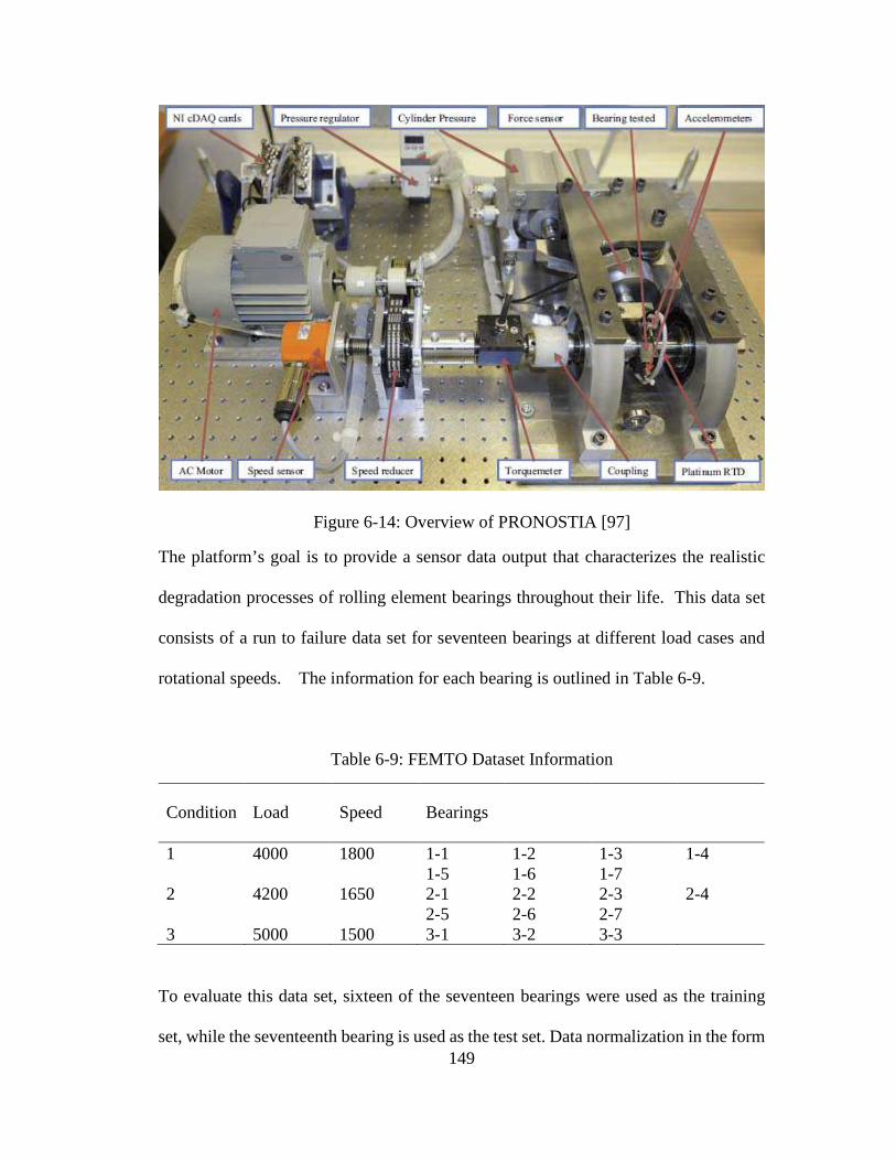
149

Figure 6-14: Overview of PRONOSTIA [97]

The platform’s goal is to provide a sensor data output that characterizes the realistic

degradation processes of rolling element bearings throughout their life. This data set

consists of a run to failure data set for seventeen bearings at different load cases and

rotational speeds. The information for each bearing is outlined in Table 6-9.

Table 6-9: FEMTO Dataset Information

Condition Load Speed Bearings

1 4000 1800 1-1 1-2 1-3 1-4 1-5 1-6 1-7 2 4200 1650 2-1 2-2 2-3 2-4 2-5 2-6 2-7 3 5000 1500 3-1 3-2 3-3

To evaluate this data set, sixteen of the seventeen bearings were used as the training

set, while the seventeenth bearing is used as the test set. Data normalization in the form

150

of spectrogram images was done to ensure a consistent signal and degradation path.

Due to the nature of this data set, only fixed interval labeling was used. Random

interval labeling was explored; however, it had mixed results. The results of the

FEMTO data set within the proposed methodology show good performance against

similar research [98], where the published RMSE results for bearings 1-3, 2-4, and 3-1

are 9.0, 8.9, and 24.2, respectively. As shown in Table 6-10, the proposed methodology

outperformed these results.

Table 6-10: FEMTO RMSE Results – Semi-supervised Feature Learning with Semi-Supervised regression.

Bearing 1% 5% 10% 20% 50% 100%

1-3 11.32 11.10 10.96 10.36 7.50 6.59 2-4 10.13 9.92 8.65 7.28 6.77 6.42 3-1 31.90 27.42 23.73 20.08 15.02 11.51

The results show the robust ability of the proposed methodology to generalize the

underlying generative function.

6.6 Conclusions

Industry 4.0 has ushered in a broadening of the structural health monitoring research

field and unsupervised RUL estimation is a critical area in this context. Many industries

are poised to benefit from this research and its ability to predict machine downtime for

planned maintenance. Many times, the data streaming from these new systems is too

difficult, time consuming, labor intensive and, therefore, costly to label. Thus, the

ability to predict remaining useful life without labels is of great economic benefit.

151

In this paper, a deep learning enabled adversarial-variational methodology, and

corresponding mathematical framework, for remaining useful life estimation was

proposed. The proposed methodology achieved superior RUL prediction performance

in terms of RMSE metric and demonstrated its ability to predict the RUL even with a

small percentage of labeled data. This methodology helps informs an engineer about

the RUL of the asset, therefore, giving them the ability to predict future maintenance

requirements before a failure occurs and make the necessary arrangements.

Within the ablation study, the proposed framework provided higher RUL prediction

performance (i.e., smaller RMSE) with a combined generative modeling methodology.

The prediction performance was further enhanced with the addition of labels to the

data set. Additionally, the type of labeling was explored and uncovered that the method

with which one labels time series can have an effect. Fixed interval labeling versus

random interval labeling will enhance or detract from one’s results.

The application of the proposed methodology is not only limited to turbo-fan engines.

Oil and gas, wind turbine farms, automotive, and aerospace can potentially benefit

from this research. While significant work was done on the neural network

architectures within this research, we believe further progress can be made by a deeper

investigation of these architectures.

152

Chapter 7: Conclusions, Contributions, and Future Research Recommendations

7.1 Conclusions

Three approaches were developed in this dissertation to address the growing need for

modeling multi-dimensional big machinery data for making maintenance decisions.

These three approaches are interrelated as a continuous process of understanding the

data and seek to answer the following research questions. If you have a large set of

labeled machinery data, can you predict a machine’s health state? If you have a large

set of unlabeled or partially labeled machinery data, can you predict a machine’s health

state? If you have a large set of unlabeled and partially labeled multi-sensor time-series

machinery degradation data, can you predict the remaining useful life?

To answer the first question, this dissertation sought to extend deep learning-based

approaches to supervised fault diagnostics. This was done with the development of a

novel deep learning framework for applications to fault diagnostics of rolling element

bearings. Within this framework, the use of time-frequency image representations of

rolling element bearings within a deep neural network architecture was pioneered.

Additionally, the proposed CNN architecture for fault diagnostics achieved superior

results while reducing the model’s learnable parameters, thus increasing the speed of

training.

Through this work, it was demonstrated that time-frequency image representations of

raw vibration signals are effective for identifying rolling element bearing fault

classification and diagnosis. The manual process of feature extraction and the delicate

153

methods of feature selection can be substituted with a deep learning framework

allowing automated feature learning for fault diagnostics. STFT, WT, and HHT images

are all shown to be effective representations of a raw signal with scalograms provided

the best diagnostic prediction accuracies. Information loss due to image scaling had

little effect on scalogram image prediction accuracies, a slight effect on the

spectrograms, and a more significant effect on the HHT images. The proposed CNN

architecture showed it is robust against injected experimental noise. Finally, the

proposed architecture delivers the same accuracies for scalogram images with lower

computational costs by reducing the number of learnable parameters.

To answer the second question, this dissertation extended semi-supervised and

unsupervised fault diagnostics with time-frequency scalogram images via a GAN-

based methodology. This work consisted of the development of a novel GANs based

framework for unsupervised and semi-supervised fault diagnostics of rolling element

bearing time-frequency scalogram image representations of the raw signal. This

included proposing neural network architectures for unsupervised and semi-supervised

fault diagnostics on the CWR and MFPT data sets within DCGAN and InfoGAN

architectures.

Through this research, it was learned GANs and deep learning-based approaches are

better able to generalize the underlying manifold space of machine health states to a

level with which a clustering algorithm can separate the healthy baseline signals with

the fault data. Both DCGAN and InfoGAN architectures are effective tools for

unsupervised fault diagnostics. Prediction accuracy results are then further improved

154

with the addition of a subset of labeled data via semi-supervised fault diagnostics. The

InfoGAN encoder vector was tested as an additional feature for clustering; however,

the addition of the encoder information had mixed results. The InfoGAN architecture

outperforms the DCGAN on noisier data like the MFPT set. DCGANs proved their

ability to diagnose faults with zero information on the real classes within the data set.

InfoGANs showed that, with slight knowledge into how many potential driving failure

modes the rolling elements may have, the diagnostics results may be efficiently

improved.

Within the published experimental results, the presented diagnostic methodologies

perform well on the two public data sets. The data sets used to evaluate this research

are limited specifically to fault classification problems. This does not evaluate how the

fault degrades to failure. This could be generalizable across multiple fault diagnosis

data sets; however, due to the computational costs of the research, one must understand

if a more sophisticated method is necessary to perform the classification task at hand.

(Each chapter went into detail with regards to computational expense.) The research

works for specific maintenance programs where, once a fault is identified, the bearing

will be replaced. This could be generalized to further classification tasks but was

beyond the scope of this research.

To answer the final research question, this dissertation sought to advance generative

modeling research and propose a novel approach to the study of the remaining useful

life prediction. This included the development of unsupervised and semi-supervised

frameworks for RUL prediction by proposing a novel non-Markovian mathematical

155

formulation combining the generative modeling strengths of both variational Bayes

and adversarial training within a state-space modeling framework. The aim was to

achieve both unsupervised and semi-supervised RUL estimation. This work concluded

a non-Markovian deep learning enabled adversarial-variational mathematical

framework is very effective in predicting the RUL of large multi-sensor assets.

Within this research, the presented prognostic methodology performs well on the two

public data sets. The data sets used to evaluate this research are limited specifically to

monotonic degradation tasks. This could be generalizable across multiple degradation-

based data sets; however, due to the computational costs of the research, one must

understand if a more sophisticated method is necessary to perform the RUL predictions.

The research works for specific maintenance programs where sensor data is tied

directly to how the asset degrades over time.

7.2 Future Research Recommendations

A limitation of the proposed methodology is inherent when trying to quantify the

variability while not specifically calculating the uncertainty. This is a potential

drawback to the presented model contributions supporting PHM risk decision making.

Therefore, a recommended future research would be to expand the three proposed

methods in terms of a Bayesian framework, so the uncertainty on fault prediction and

RUL can be explicitly calculated. This approach would be useful with the implication

of a quantifiable uncertainty metric where an objective function could find a relation

between the percentage of labeling and the uncertainty on RUL. From this, one could

156

then find an optimal labeling percentage for a given physical asset’s dataset based on

the risk surrounding a failed prediction versus the engineering cost to label more data.

For time-based prediction methodologies, there are a few standard evaluation metrics

recognized by the research community. This research did not explore the limitations

of the metrics, nor did it propose a new one. Further research should be done in the

future around development of more appropriate evaluation metrics for time-based

prediction methodologies.

Another limitation of this work is encoded within the basis of time series predictions

for deep learning-based methodologies. Time series data must arrive at constant

intervals in order to predict future health states. This limits the use of these

methodologies to continuous data; therefore, it eliminates the ability to incorporate

transient signal prediction capabilities (e.g., acoustic emission-based). Therefore,

another future research suggestion would be to expand the three proposed

methodologies to include ordinary differential equations, which have recently emerged

as a possible solution to this problem and show great promise for intermittent signals.

Finally, the dissertation was limited to modeling methods which did not incorporate

physics directly into the modeling and would be another drawback in supporting PHM-

based risk decision making. Thus, it would be advantageous to add a framework into

this research for the remaining useful life estimation through a physics-informed

framework.

157

Bibliography [1] Si, Xiao-Sheng, et al. "Remaining useful life estimation–a review on the

statistical data driven approaches." European journal of operational research

213.1 (2011): 1-14.

[2] Verstraete, D.B., Droguett, E.L., Ferrada, A. Meruane, V, Modarres, M. (2018)

“Unsupervised deep generative adversarial based methodology for automatic

fault detection” In Haugen, S. (Ed.), Barros, A. (Ed.), Gulijk, C. v. (Ed.),

Kongsvik, T. (Ed.), Vinnem, J. (Ed.). (2018). Safety and Reliability – Safe

Societies in a Changing World. London: CRC Press.

[3] Huo, Z., Zhang, Y., Francq, P., Shu, L., Huang, J., & others. (2017). Incipient

fault diagnosis of roller bearing using optimized wavelet transform based multi-

speed vibration signatures. IEEE Access.

[4] Wang, J., Duan, L., Zhuang, J., & Chang, W. (2016). “A Multi-Scale

Convolutional Neural Network for Featureless Fault Diagnosis.” 2016

International Symposium on Flexible Automation. (pp. 1–3).

[5] Seera, M., & Lim, C. P. (2016). Online motor fault detection and diagnosis

using a hybrid FMM-CART model. IEEE Transactions on Neural Networks

and Learning Systems, 25(4), 806–812.

[6] Loparo, K. A., Bearing Data Center, Case Western Reserve University, 2013,

http://csegroups.case.edu/bearingdatacenter/pages/welcome-case-western-

reserve-university-bearing-data-center-website. December 2, 2018.

158

[7] Sharma, Aditya, M. Amarnath, and P. K. Kankar. "Feature extraction and fault

severity classification in ball bearings." Journal of Vibration and Control 22.1

(2016): 176-192.

[8] Wong, P. K., Zhong, J., Yang, Z., & Vong, C. M. (2016). Sparse Bayesian

extreme learning committee machine for engine simultaneous fault diagnosis.

Neurocomputing, 174, 331–343.

[9] LeCun, Y., Bengio, Y., & Hinton, G. (2015). Deep learning. Nature, 521(7553),

436–444.

[10] Szegedy, Christian, et al. "Going deeper with convolutions." Proceedings of the

IEEE Conference on Computer Vision and Pattern Recognition. 2015.

[11] Tompson, J., Goroshin, R., Jain, A., Lecun, Y., & Bregler, C. (2015). “Efficient

Object Localization Using Convolutional Networks.”

https://arxiv.org/abs/1411.4280

[12] Taigman, Yaniv, et al. "Deepface: Closing the gap to human-level performance

in face verification." Proceedings of the IEEE Conference on Computer Vision

and Pattern Recognition. 2014.

[13] Sermanet, P., Eigen, D., Zhang, X., Mathieu, M., Fergus, R., & LeCun, Y.

(2013). OverFeat: Integrated Recognition, Localization and Detection using

Convolutional Networks. arXiv Preprint arXiv, 1312.6229.

[14] Girshick, R., Donahue, J., Darrell, T., & Malik, J. (2014). Rich feature

hierarchies for accurate object detection and semantic segmentation.

Proceedings of the IEEE Computer Society Conference on Computer Vision

and Pattern Recognition, 580–587.

159

[15] Simonyan, K., & Zisserman, A. (2015). Very Deep Convolutional Networks for

Large-Scale Image Recognition. International Conference on Learning

Representations (ICRL), 1–14.

[16] Cires, D., & Meier, U. (2012). Multi-column Deep Neural Networks for Image

Classification. IEEE Conference on Computer Vision and Pattern Recognition,

(February), 3642–3649.

[17] Krizhevsky, A., Sutskever, I., & Geoffrey E., H. (2012). ImageNet

Classification with Deep Convolutional Neural Networks. Advances in Neural

Information Processing Systems 25 (NIPS2012), 1–9.

[18] Guo, X., Chen, L., and Shen, C., “Hierarchical adaptive deep convolution

neural network and its application to bearing fault diagnosis,” Measurement,

vol. 93, pp. 490–502, 2016.

[19] Lee, D., Siu, V., Cruz, R., & Yetman, C. (2016). Convolutional Neural Net and

Bearing Fault Analysis, 194–200.

[20] Abdeljaber, O., Avci, O., Kiranyaz, S., Gabbouj, M., & Inman, D. J. (2017).

”Real-time vibration-based structural damage detection using one-dimensional

convolutional neural networks. ” Journal of Sound and Vibration, 388, 154–

170.

[21] Janssens, O., Slavkovikj, V., Vervisch, B., Stockman, K., Loccufier, M.,

Verstockt, S., … Van Hoecke, S. (2016). Convolutional Neural Network Based

Fault Detection for Rotating Machinery. Journal of Sound and Vibration, 377,

331–345.

160

[22] Chen, Z., Li, C., & Sanchez, R. (2015). Gearbox Fault Identification and

Classification with Convolutional Neural Networks. Shock and Vibration,

2015.

[23] Zhang, C., Lim, P., Qin, A. K., & Tan, K. C. (2016). ”Multiobjective Deep

Belief Networks Ensemble for Remaining Useful Life Estimation in

Prognostics. ” IEEE Transactions on Neural Networks and Learning Systems,

PP(99), 1–13.

[24] Liao, Linxia, Wenjing Jin, and Radu Pavel. (2016) "Enhanced restricted

boltzmann machine with prognosability regularization for prognostics and

health assessment." IEEE Transactions on Industrial Electronics 63.11: 7076-

7083.

[25] Babu, Giduthuri Sateesh, Peilin Zhao, and Xiao-Li Li. "Deep convolutional

neural network based regression approach for estimation of remaining useful

life." International Conference on Database Systems for Advanced

Applications. Springer International Publishing, 2016.

[26] Guo, L., Gao, H., Huang, H., He, X., & Li, S. (2016). “Multifeatures Fusion

and Nonlinear Dimension Reduction for Intelligent Bearing Condition

Monitoring.” Shock and Vibration, 2016.

[27] Zhou, Funa, Yulin Gao, and Chenglin Wen. "A Novel Multimode Fault

Classification Method Based on Deep Learning." Journal of Control Science

and Engineering 2017 (2017).

[28] Liu, Hongmei, Lianfeng Li, and Jian Ma. "Rolling bearing fault diagnosis based

on stft-deep learning and sound signals." Shock and Vibration 2016 (2016).

161

[29] Bouvrie, Jake. "Notes on convolutional neural networks." (2006).

[30] Feng, Z., Liang, M., & Chu, F. (2013). Recent advances in time-frequency

analysis methods for machinery fault diagnosis: A review with application

examples. Mechanical Systems and Signal Processing, 38(1), 165–205.

[31] Lin, Jing, and Liangsheng Qu. "Feature extraction based on Morlet wavelet and

its application for mechanical fault diagnosis." Journal of sound and vibration

234.1 (2000): 135-148.

[32] Peng, Z. K., and F. L. Chu. "Application of the wavelet transform in machine

condition monitoring and fault diagnostics: a review with bibliography."

Mechanical systems and signal processing 18.2 (2004): 199-221.

[33] Huang, Norden Eh. “Hilbert-Huang transform and its applications.” Vol. 16.

World Scientific, 2014.

[34] Meeson Jr., R. N. (2005). HHT sifting and filtering. Hilbert-Huang Transform

and Its Applications, 5, 75–105.

[35] Smith, J. S. (2005). The local mean decomposition and its application to EEG

perception data. Journal of The Royal Society Interface, 2(5), 443–454.

[36] Kingma, Diederik, and Jimmy Ba. "Adam: A method for stochastic

optimization." arXiv preprint arXiv:1412.6980 (2014).

[37] Bechhoefer, Eric. "A Quick Introduction to Bearing Envelope Analysis."

(2016).

[38] MFPT Data Set, http://www.mfpt.org/FaultData/FaultData.htm.

162

[39] Raveendran, H., Deepa Thomas. "Image Fusion Using LEP Filtering and

Bilinear Interpolation", International Journal of Engineering Trends and

Technology (IJETT), V12(9),427-431 June 2014. ISSN:2231-5381.

[40] Sokolova, M., & Lapalme, G. (2009). “A systematic analysis of performance

measures for classification tasks.” Information Processing and Management,

45, p. 427-437.

[41] Smith, Wade A., and Robert B. Randall. "Rolling element bearing diagnostics

using the Case Western Reserve University data: A benchmark study."

Mechanical Systems and Signal Processing 64 (2015): 100-131.

[42] Langone, R., Reynders, E., Mehrkanoon, S., & Suykens, J. A. K. (2016).

Automated structural health monitoring based on adaptive kernel spectral

clustering, 90(June), 1–21. https://doi.org/10.1016/j.ymssp.2016.12.002

[43] L. Wang, X. Zhao, J. Pei, and G. Tang, “Transformer fault diagnosis using

continuous sparse autoencoder,” SpringerPlus, vol. 5, no. 1, p. 1, 2016.

[44] Lei, Y., Jia, F., Lin, J., Xing, S., & Ding, S. X. (2016). An Intelligent Fault

Diagnosis Method Using Unsupervised Feature Learning Towards Mechanical

Big Data. IEEE Transactions on Industrial Electronics, 63(5), 3137–3147.

https://doi.org/10.1109/TIE.2016.2519325

[45] Jiang, Peng, et al. "Fault diagnosis based on chemical sensor data with an active

deep neural network." Sensors 16.10 (2016): 1695.

[46] Sun, Wenjun, et al. "A sparse auto-encoder-based deep neural network

approach for induction motor faults classification." Measurement 89 (2016):

171-178.

163

[47] Goodfellow, I., Pouget-Abadie, J., Mirza, M., Xu, B., Warde-Farley, D., Ozair,

S., … Bengio, Y. (2014). Generative Adversarial Nets. Advances in Neural

Information Processing Systems 27, 2672–2680.

[48] Verstraete, D., Ferrada, A., Droguett, E. L., Meruane, V., & Modarres, M.

(2017). Deep Learning Enabled Fault Diagnosis Using Time-Frequency Image

Analysis of Rolling Element Bearings. Shock and Vibration, 2017.

[49] Radford, A., Metz, L., & Chintala, S. (2016). Unsupervised Representation

Learning with Deep Convolutional Generative Adversarial Networks. arXiv, 1–

15.

[50] Ioffe, Sergey, and Christian Szegedy. "Batch normalization: Accelerating deep

network training by reducing internal covariate shift." International Conference

on Machine Learning. 2015.

[51] Christopher D. Manning, Prabhakar Raghavan, and Hinrich Schütze.

2008. Introduction to Information Retrieval. Cambridge University Press, New

York, NY, USA.

[52] Kuncheva, Ludmila I. Combining pattern classifiers: methods and algorithms.

John Wiley & Sons, 2004.

[53] Hubert, Lawrence, and Phipps Arabie. "Comparing partitions." Journal of

classification 2.1 (1985): 193-218.

[54] Gugulothu, https://arxiv.org/abs/1709.01073

[55] Malhotra, P., TV, V., Ramakrishnan, A., Anand, G., Vig, L., Agarwal, P., &

Shroff, G. (2016). Multi-Sensor Prognostics using an Unsupervised Health

164

Index based on LSTM Encoder-Decoder. Retrieved from

http://arxiv.org/abs/1608.06154

[56] Zhao, R., Wang, J., Yan, R., & Mao, K. (2016). Machine health monitoring

with LSTM networks. Proceedings of the International Conference on Sensing

Technology, ICST.

[57] Yuan, Mei, Yuting Wu, and Li Lin. "Fault diagnosis and remaining useful life

estimation of aero engine using lstm neural network." Aircraft Utility Systems

(AUS), IEEE International Conference on. IEEE, 2016.

[58] Zheng, S., Ristovski, K., Farahat, A., & Gupta, C. (2017). Long Short-Term

Memory Network for Remaining Useful Life estimation. 2017 IEEE

International Conference on Prognostics and Health Management (ICPHM),

88–95.

[59] Wu, Y., Yuan, M., Dong, S., Lin, L., & Liu, Y. (2017). Remaining useful life

estimation of engineered systems using vanilla LSTM neural networks.

Neurocomputing, 0, 1–13.

[60] Aydin, O., & Guldamlasioglu, S. (2017). Using LSTM networks to predict

engine condition on large scale data processing framework. 2017 4th

International Conference on Electrical and Electronics Engineering, ICEEE

2017, 281–285.

[61] Zhao, Guangquan, et al. "Lithium-ion battery remaining useful life prediction

with Deep Belief Network and Relevance Vector Machine." Prognostics and

165

Health Management (ICPHM), 2017 IEEE International Conference on. IEEE,

2017.

[62] Ren, L., Cui, J., Sun, Y., & Cheng, X. (2017). Multi-bearing remaining useful

life collaborative prediction: A deep learning approach. Journal of

Manufacturing Systems, 43, 248–256.

[63] Li, X., Ding, Q., & Sun, J.-Q. (2017). Remaining Useful Life Estimation in

Prognostics Using Deep Convolution Neural Networks. Reliability Engineering

& System Safety, 172(November 2017), 1–11.

[64] Nash, John F. "Equilibrium points in n-person games." Proceedings of the

national academy of sciences 36.1 (1950): 48-49.

[65] San Martin, Gabriel, et al. "Deep variational auto-encoders: A promising tool

for dimensionality reduction and ball bearing elements fault diagnosis."

Structural Health Monitoring (2018): 1475921718788299.

[66] Kingma, Diederik P., and Max Welling. "Auto-encoding variational bayes."

arXiv preprint arXiv:1312.6114 (2013).

[67] Frederick, Dean K., Jonathan A. DeCastro, and Jonathan S. Litt. "User's guide

for the commercial modular aero-propulsion system simulation (C-MAPSS)."

(2007).

[68] Modarres, C., Coburger, A., Droguett, E. L., & Fuge, M. (2017). Computer

Vision for Damage Recognition and Type Identification: A Deep Learning

Based Approach, ESREL 2017.

166

[69] Li, Xiang, Qian Ding, and Jian-Qiao Sun. "Remaining useful life estimation in

prognostics using deep convolution neural networks." Reliability Engineering

& System Safety 172 (2018): 1-11.

[70] Lee, S., Ha, J., Zokhirova, M. et al. Arch Computat Methods Eng (2018) 25:

121. https://doi.org/10.1007/s11831-017-9237-0

[71] Jiang, Peng, et al. "Fault diagnosis based on chemical sensor data with an active

deep neural network." Sensors 16.10 (2016): 1695.

[72] Sun, Wenjun, et al. "A sparse auto-encoder-based deep neural network

approach for induction motor faults classification." Measurement 89 (2016):

171-178.

[73] L. Liao, W. Jin, and R. Pavel, “Enhanced restricted Boltzmann machine with

prognosability regularization for prognostics and health assessment,” IEEE

Transactions on Industrial Electronics, vol. 63, no. 11, 2016.

[74] Wang, Jinyong, and Ce Zhang. "Software reliability prediction using a deep

learning model based on the RNN encoder–decoder." Reliability Engineering

& System Safety 170 (2018): 73-82.

[75] Arthur, David, and Sergei Vassilvitskii. "k-means++: The advantages of careful

seeding." Proceedings of the eighteenth annual ACM-SIAM symposium on

Discrete algorithms. Society for Industrial and Applied Mathematics, 2007.

[76] Shi, Jianbo, and Jitendra Malik. "Normalized cuts and image segmentation."

Departmental Papers (CIS) (2000): 107.

[77] Metz, Luke, et al. "Unrolled generative adversarial networks." arXiv preprint

arXiv:1611.02163 (2016).

167

[78] Chen, Xi, et al. "Infogan: Interpretable representation learning by information

maximizing generative adversarial nets." Advances in Neural Information

Processing Systems. 2016.

[79] Salimans, Tim, et al. "Improved techniques for training gans." Advances in

Neural Information Processing Systems. 2016.

[80] Jebara T. (2004) Generative Versus Discriminative Learning. In: Machine

Learning. The International Series in Engineering and Computer Science,

vol 755. Springer, Boston, MA

[81] Odena, Augustus, Vincent Dumoulin, and Chris Olah. "Deconvolution and

checkerboard artifacts." Distill 1.10 (2016): e3.

[82] Zhao, R., Yan, R., Wang, J., & Mao, K. (2017). Learning to monitor machine

health with convolutional Bi-directional LSTM networks. Sensors

(Switzerland), 17(2), 1–19.

[83] Ellefsen, André Listou, et al. "Remaining useful life predictions for turbofan

engine degradation using semi-supervised deep architecture." Reliability

Engineering & System Safety 183 (2019): 240-251.

[84] Ren, L., Cui, J., Sun, Y., & Cheng, X. (2017). Multi-bearing remaining useful

life collaborative prediction: A deep learning approach. Journal of

Manufacturing Systems, 43, 248–256.

[85] Li, X., Ding, Q., & Sun, J.-Q. (2017). Remaining Useful Life Estimation in

Prognostics Using Deep Convolution Neural Networks. Reliability Engineering

& System Safety, 172(November 2017), 1–11.

168

[86] Bayer, Justin, and Christian Osendorfer. "Learning stochastic recurrent

networks." arXiv preprint arXiv:1411.7610 (2014).

[87] Chung, Junyoung, et al. "A recurrent latent variable model for sequential data."

Advances in neural information processing systems. 2015.

[88] Krishnan, Rahul G., Uri Shalit, and David Sontag. "Structured inference

networks for nonlinear state space models." Thirty-First AAAI Conference on

Artificial Intelligence. 2017.

[89] Karl, Maximilian, et al. "Deep variational bayes filters: Unsupervised learning

of state space models from raw data." arXiv preprint arXiv:1605.06432 (2016).

[90] Mescheder, Lars, Sebastian Nowozin, and Andreas Geiger. "Adversarial

variational bayes: Unifying variational autoencoders and generative adversarial

networks." Proceedings of the 34th International Conference on Machine

Learning-Volume 70. JMLR. org, 2017.

[91] Hu, Zhiting, et al. "On unifying deep generative models." arXiv preprint

arXiv:1706.00550 (2017).

[92] Hinton, Geoffrey E., et al. "The" wake-sleep" algorithm for unsupervised neural

networks." Science 268.5214 (1995): 1158-1161.

[93] A. Saxena, K. Goebel, D. Simon, and N. Eklund, “Damage Propagation

Modeling for Aircraft Engine Run-to-Failure Simulation”, in the Proceedings

of the Ist International Conference on Prognostics and Health Management

(PHM08), Denver CO, Oct 2008.

[94] Yoon, Andre S., et al. "Semi-supervised learning with deep generative models

for asset failure prediction." arXiv preprint arXiv:1709.00845 (2017).

169

[95] Huang, Yu, et al. "An Adversarial Learning Approach for Machine Prognostic

Health Management." 2019 International Conference on High Performance

Big Data and Intelligent Systems (HPBD&IS). IEEE, 2019.

[96] Castrejon, Lluis, Nicolas Ballas, and Aaron Courville. "Improved Conditional

VRNNs for Video Prediction." arXiv preprint arXiv:1904.12165 (2019).

[97] Nectoux, Patrick, et al. "PRONOSTIA: An experimental platform for bearings

accelerated degradation tests." IEEE International Conference on Prognostics

and Health Management, PHM'12.. IEEE Catalog Number: CPF12PHM-

CDR, 2012.

[98] Li, Xiang, Wei Zhang, and Qian Ding. "Deep learning-based remaining useful

life estimation of bearings using multi-scale feature extraction." Reliability

Engineering & System Safety 182 (2019): 208-218.

abstract dissertation: deep adversarial approaches in

Documents