ABSTRACT

Title of dissertation: Combinatorial Problems in Online Advertising

Azarakhsh Malekian, Doctor of Philosophy, 2009

Dissertation directed by: Professor Samir KhullerDepartment of Computer Science

Electronic commerce or eCommerce refers to the process of buying and selling ofgoods and services over the Internet. In fact, the Internet has completely transformedtraditional media based advertising so much so that billions of dollars of advertisingrevenue is now flowing to search companies such as Microsoft, Yahoo! and Google.In addition, the new advertising landscape has opened up the advertising industryto all players, big and small. However, this transformation has led to a host of newproblems faced by the search companies as they make decisions about how much tocharge for advertisements, whose ads to display to users, and how to maximize theirrevenue. In this thesis we focus on an entire suite of problems motivated by thecentral question of “Which advertisement to display to which user?”.

Targeted advertisement happens when a user enters a relevant search query. Theads are usually displayed on the sides of the search result page. Internet advertisingalso takes place by displaying ads on the side of webpages with relevant content. Whilelarge advertisers (e.g. Coca Cola) pursue brand recognition by advertisement, smalladvertisers are happy with instant revenue as a result of a user following their ad andperforming a desired action (e.g. making a purchase). Therefore, small advertisersare often happy to get any ad slot related to their ad while large advertisers prefercontracts that will guarantee that their ads will be delivered to enough number ofdesired users. We first focus on two problems that come up in the context of smalladvertisers.

The first problem we consider deals with the allocation of ads to slots consideringthe fact that users enter search queries over a period of time, and as a result the slotsbecome available gradually. We use a greedy method for allocation and show that

the online ad allocation problem with a fixed distribution of queries over time can bemodeled as maximizing a continuous non-decreasing submodular sequence functionfor which we can guarantee a solution with a factor of at least (1−1/e) of the optimal.

The second problem we consider is query rewriting problem in the context ofkeyword advertisement. This problem can be posed as a family of graph coveringproblems to maximize profit. We obtain constant-factor approximation algorithmsfor these covering problems under two sets of constraints and a realistic notion ofad benefit. We perform experiments on real data and show that our algorithms arecapable of outperforming a competitive baseline algorithm in terms of the benefit dueto rewrites.

We next consider two problems related to premium customers, who need guaran-teed delivery of a large number of ads for the purpose of brand recognition and wouldrequire signing a contract. In this context, we consider the allocation problem withthe objective of maximizing either revenue or fairness.

The problems considered in this thesis address just a few of the current challengesin e-Commerce and Internet Advertising. There are many interesting new problemsarising in this field as the technology evolves and online-connectivity through inter-active media and the internet become ubiquitous. We believe that this is one of theareas that will continue to receive greater attention by researchers in the near future.

Combinatorial Problems in Online Advertising

by

Azarakhsh Malekian

Dissertation submitted to the Faculty of the Graduate School of theUniversity of Maryland, College Park in partial fulfillment

of the requirements for the degree ofDoctor of Philosophy

2009

Advisory Committee:Professor Samir Khuller, Chair/AdvisorProfessor Lawrence AusubelProfessor David MountProfessor Neil SpringProfessor Aravind Srinivasan

c© Copyright byAzarakhsh Malekian

2009

Dedication

This thesis is dedicated to my parents Mahindokht and Abdolali. I would not

have been able to accomplish this without their endless love and earnest support. I

owe them for all of my achievements

ii

Acknowledgments

This thesis could not have been accomplished without the assistance of many

teachers, colleagues and friends.

I would first like to thank my advisor, Professor Samir Khuller for his guidance

and support throughout my graduate career and during the completion of this thesis.

Samir let me have the freedom to pursue my interests and work on problems that were

more appealing to me in algorithm design. At the same time, he helped me clarify

my ideas and patiently advised me on how to improve my skills. I am also extremely

grateful to the members of my committee, Professor Lawrence Ausubel, Professor

David Mount, Professor Neil Spring and Professor Aravind Srinivasan for taking the

time to be in my thesis committee and for giving me very useful comments. I am in

debt to all of them for their advices during the writing of my thesis and throughout

the years I was in graduate school.

I was lucky to be a part of a friendly department. I should thank all my friends,

staff and officemates for providing such a nice atmosphere. Special thanks to my

friend and collaborator Saeed with whom we worked on a lot of problems and learned

a lot. Also I should thank my colleagues Julian Mestre, Yoo Ah kim and Mohammad

Toossi for sharing their insightful ideas and Co-authoring papers with me. I should

also thank Professor Amol Deshpande for sharing his ideas and co-authoring a paper

iii

with me. I owe my gratitude to kind staff of computer science department, specially

Jennifer Story and Fatima Bangura for all their help and support.

During my years at UMD, I visited Yahoo! and Microsoft Research. These visits

opened up my mind into new fascinating problems and gave me the opportunity

to collaborate with many brilliant researchers. Special thanks to Ravi Kumar and

Mohammad Mahdian, Grant Want and Chi Chao Chang and Erik Vee from Yahoo!

and Adam Kalai, Christian Borgs and Jennifer Chayes from Microsoft Research. I

also should thank Professor Jason Hartline for all his useful advices.

Studying all these years in graduate school, far from home, would not have been

possible without the support and sympathy of all my friends. Many thanks to all my

dear friends specially my dear Baharak.

The work in this dissertation was done under the support of the NSF grant CCF-

0430650 which I am duly grateful.

Before coming to University of Maryland, I spent my undergrad at Sharif Univer-

sity of Technology. I would like to thank Professor Mohammad Ghodsi who intro-

duced me theoretical computer science and helped me build up my background.

Last but not the least, my dear parents and family receive my most heartful

gratitude for their endless love. I want to thank my sister Azadeh and my brother

Roozbeh for their support and love all these years.

iv

This thesis is dedicated to my parents Mahindokht and Abdolali whom I cannot

think of a proper way of thanking them compared to all their endless support and

love. I owe them for all of my achievements.

v

Table of Contents

List of Tables viii

List of Figures ix

1 Introduction 11.1 Problem Formulation . . . . . . . . . . . . . . . . . . . . . . . . . . . 8

1.1.1 Online Ad Allocation Problem . . . . . . . . . . . . . . . . . . 81.1.2 Query Rewriting Problem . . . . . . . . . . . . . . . . . . . . 91.1.3 Online Ad allocation for Display advertisement . . . . . . . . 121.1.4 Fair Contract Allocation: . . . . . . . . . . . . . . . . . . . . . 13

1.2 Roadmap . . . . . . . . . . . . . . . . . . . . . . . . . . . . . . . . . 16

2 Background and Related Work 182.1 Submodular Functions . . . . . . . . . . . . . . . . . . . . . . . . . . 182.2 Online Allocation Problem . . . . . . . . . . . . . . . . . . . . . . . . 192.3 Query Rewriting . . . . . . . . . . . . . . . . . . . . . . . . . . . . . 202.4 Display Advertisement . . . . . . . . . . . . . . . . . . . . . . . . . . 202.5 Fair Allocation . . . . . . . . . . . . . . . . . . . . . . . . . . . . . . 212.6 Online Resource Allocation . . . . . . . . . . . . . . . . . . . . . . . . 21

3 Non-guaranteed Delivery: Online Ad Allocation Problem 243.1 Sequence Submodularity . . . . . . . . . . . . . . . . . . . . . . . . . 253.2 Definitions . . . . . . . . . . . . . . . . . . . . . . . . . . . . . . . . . 26

3.2.1 Submodular Non-decreasing Sequence Functions . . . . . . . . 293.3 Greedy Heuristic (Discrete) . . . . . . . . . . . . . . . . . . . . . . . 293.4 Greedy Heuristic (Continuous) . . . . . . . . . . . . . . . . . . . . . . 323.5 Online ad allocation problem . . . . . . . . . . . . . . . . . . . . . . . 36

4 Query Rewriting for Keyword-based Advertising 404.1 Why rewrite queries for keyword advertising? . . . . . . . . . . . . . 404.2 Formulation . . . . . . . . . . . . . . . . . . . . . . . . . . . . . . . . 414.3 Algorithms for cardinality version . . . . . . . . . . . . . . . . . . . . 44

4.3.1 Warmup: Single query case . . . . . . . . . . . . . . . . . . . 444.3.2 The general case . . . . . . . . . . . . . . . . . . . . . . . . . 464.3.3 Hardness results for Cardinality Version . . . . . . . . . . . . 484.3.4 Tight examples for cardinality version . . . . . . . . . . . . . . 49

vi

4.4 Algorithm for the weighted version . . . . . . . . . . . . . . . . . . . 514.5 Experimental results . . . . . . . . . . . . . . . . . . . . . . . . . . . 52

4.5.1 Editorial relevance . . . . . . . . . . . . . . . . . . . . . . . . 534.5.2 d-benefit . . . . . . . . . . . . . . . . . . . . . . . . . . . . . . 54

4.5.2.1 Comparing Single-Query-Greedy and Baseline 54

5 Guaranteed Delivery Advertisement: Fair Allocation With a Compact Plan 595.1 Fair Allocation with a Compact Plan . . . . . . . . . . . . . . . . . . 59

5.1.1 Fair allocation with L1 penalty . . . . . . . . . . . . . . . . . 605.1.2 Reconstruction for L1 . . . . . . . . . . . . . . . . . . . . . . . 62

5.1.2.1 Computing the plan . . . . . . . . . . . . . . . . . . 645.1.2.2 Reconstruction using the plan . . . . . . . . . . . . . 67

5.1.3 Effect of supply scaling . . . . . . . . . . . . . . . . . . . . . . 695.1.4 Convex penalty functions . . . . . . . . . . . . . . . . . . . . . 705.1.5 A greedy solution for L1 allocation with soft demand . . . . . 73

5.1.5.1 Reconstructing the greedy solution . . . . . . . . . . 74

6 Guaranteed Delivery Advertisement: Online Ad Allocation 756.1 Online Setting . . . . . . . . . . . . . . . . . . . . . . . . . . . . . . . 75

6.1.1 Definitions and Settings . . . . . . . . . . . . . . . . . . . . . 766.1.2 Online Algorithm . . . . . . . . . . . . . . . . . . . . . . . . . 77

6.1.2.1 Lower Bounds . . . . . . . . . . . . . . . . . . . . . . 786.1.2.2 The online Algorithm . . . . . . . . . . . . . . . . . 79

6.1.3 Simulation . . . . . . . . . . . . . . . . . . . . . . . . . . . . . 84

7 Conclusion and Future Work 887.1 Future Work . . . . . . . . . . . . . . . . . . . . . . . . . . . . . . . . 91

Bibliography 94

vii

List of Tables

4.3 d-benefit: Percentage gain of Algorithm Single-Query-Greedy overAlgorithm Baseline broken down by |W |. . . . . . . . . . . . . . . . 56

4.1 Relevance comparison: Algorithm Baseline vs. Algorithm Single-Query Greedy . . . . . . . . . . . . . . . . . . . . . . . . . . . . . 58

4.2 d-benefit: Percentage gain of Algorithm Single-Query-Greedy overAlgorithm Baseline. . . . . . . . . . . . . . . . . . . . . . . . . . . . 58

6.1 Results for the first dataset . . . . . . . . . . . . . . . . . . . . . . . 85

6.2 Results for the second dataset . . . . . . . . . . . . . . . . . . . . . . 85

6.3 Results for the third dataset . . . . . . . . . . . . . . . . . . . . . . . 85

6.4 Results for the fourth dataset . . . . . . . . . . . . . . . . . . . . . . 86

6.5 Parameters of the datasets . . . . . . . . . . . . . . . . . . . . . . . . 86

6.6 Performance of the Integer Program solution . . . . . . . . . . . . . . 87

viii

List of Figures

1.1 Traditional methods for advertising . . . . . . . . . . . . . . . . . . . 2

1.2 Advertisement for the search query “flower” . . . . . . . . . . . . . . 4

1.3 Three layer graph containing queries, rewrites and ads . . . . . . . . 11

1.4 It is not feasible to give each contract its completely representativeallocation . . . . . . . . . . . . . . . . . . . . . . . . . . . . . . . . . 15

1.5 Organization . . . . . . . . . . . . . . . . . . . . . . . . . . . . . . . 17

4.1 three layer graph containing queries, rewrites and ads . . . . . . . . . 42

4.2 Tight example for the general cardinality case . . . . . . . . . . . . . 50

5.1 The network construction, with (capacity, cost) on the edges. . . . . . 61

5.2 Tight example for Theorem 7. . . . . . . . . . . . . . . . . . . . . . 70

5.3 The network construction, with (capacity, cost) on the edges for L22. . 71

6.1 ORA . . . . . . . . . . . . . . . . . . . . . . . . . . . . . . . . . . . . 79

ix

Chapter 1Introduction

Advertising is a key factor in marketing; since it benefits both sellers and buyers.From the seller’s point of view, advertising is a means of introducing new productsto the world and describing their new features and also what makes them uniquecompared to other products available in the market. At the same time, it can helpbuyers decide which products match their needs the best, since they learn about moreoptions to choose from. For example, consider a company that has an opening for aposition. By advertising the position, the company gets more interested applicantsand can possibly find a better match for its position. Furthermore, advertising helpsapplicants not to miss an opportunity simply by being unaware of all relevant openpositions. Advertising is usually done many forms of media. It can be in the form ofdisplaying advertisement as a wall painting, a TV commercial, a newspaper ad, etc.(Figure 1.1).

In the past few years, advertising over the Internet has overtaken many of the“traditional” media outlets because of the shift toward people’s usage of the Internetfor entertainment, communication, and as the main resource for information. Inaddition, the new features of advertising over the Internet make it more and moredesirable for advertisers. First of all, Internet advertising lets the advertisers showtheir ad to targeted users of a random sample of the population. One way of targetedadvertising instead, is by showing the ad only to a subset of users who are searchingfor a specific keyword. For example a travel agency would rather to show their adto a person who is searching for something related to traveling such as plane ticketsand hotels. instead of a random user. Most search engine companies are showing adsbased on search terms we enter into the search engine. Another way is by targeting adsbased on factors such as gender, age, geographic location and other general factors.

Another advantage of Internet advertising is cost. Considering the cost againstthe reach of interested audience, it is relatively cheaper than other media. The natureof the medium allows consumers to research and purchase products and services attheir own convenience. At the same time, it is much easier and cheaper to collectaccurate statistical data on the effectiveness of the advertisement over the audienceand it can help advertisers to find the best way of advertising and best subgroupof the audience to target. The advertisers can choose different methods for payingfor ads: pay per impression in which an advertiser will be charged when her ad isshown to a user, pay per click in which an advertiser is charged only when a user

1

Billboard Advertising

Wall Painting

Figure 1.1: Traditional methods for advertising

2

clicks on her ad, or pay per action in which the advertiser is charged only when auser performs a desired action (e.g., purchases the product). By choosing pay perclick or pay per action, advertisers can quickly measure the effectiveness by countingthe clicks or actions. However such measurements cannot be achieved through massmedia or billboard advertising, where an individual will at best be interested, andthen decide to obtain more information about the product at a later time.

The focus of this dissertation is online targeted advertising, and some of theoptimization problems that Internet advertising companies face. We consider prob-lems with the main objective of profit maximization for these companies as well asconsumer satisfaction. What makes these problems unique from the combinatorialperspective is the volume of trades that can happen simultaneously. Furthermore,the speed of running the actions, the number of participants in each trade and theanonymity of the participants are other reasons for making the problems distinctive.Because of these special properties, the usual solutions might not be feasible or evena good solution anymore.

From the perspective of the Internet advertising companies, such as Google orYahoo!, online advertising can be categorized to two main classes:

• Non-Guaranteed Delivery

• Guaranteed Delivery

Non-Guaranteed Delivery is the traditional way of online advertising over theInternet. In this variant, advertisers ask to show their ad for a slot, for queriessearched by Internet users one by one (query is a set of keywords that a user isinterested in). The main property of this variant is that the allocation and paymentis computed online for each query separately (Figure 1.2).

Various auction formats might be used for doing the allocation and charging theadvertisers. Almost all of them have the following format: Advertisers submit bidsto the auction to win a slot on a search result page. The auction has the propertythat larger bids will have a higher chance of getting top slots. Each advertiser ischarged based on the number of clicks by users on their ads and the position of theslot they get. The bid value submitted by each advertiser defines their valuation fora single click. Each advertiser can also submit their daily or monthly budget andask the search engine to include them in the upcoming auctions for their desiredkeyword as long as they are within their budget limit. As the most popular method,we describe the Generalized Second Price auction, currently used in Google AdWordsand Yahoo! Search Marketing. In this method, the search engine (e.g., Google)runs a separate auction for each incoming query. This is an internal process andadvertisers submit their keyword, their bid and budget only once to the search engine.

3

Sponsored Links (Advertisements)query =flower

Slots for query

Figure 1.2: Advertisement for the search query “flower”

4

The search engine assigns a weight to each (advertiser, keyword) pair based on theexpected relevance. The weight is independent of the advertiser’s submitted bid. Inthe auction, advertisers are ranked based on the product of their weight and theirbid. Next, each advertiser is charged equal to the minimum bid that she could submitand still win the same slot.

Another category of online advertising that is more popular for banner adver-tisement is Guaranteed Delivery Advertisement. In the past, most banner ad-vertisements were sold through negotiation between advertisers and publishers (websites) that could result in inefficient outcomes and higher costs. In recent years,there has been some effort on automating this process, called Guaranteed Delivery.Guaranteed Delivery was introduced and implemented in major search engines likeYahoo! and Google for dealing with banner advertising. In guaranteed delivery, eachadvertiser specifies a collection of host web pages (publishers) based on the relevanceto her product. They also specify the desired total number of impressions on thesepages, and a maximum price that they are willing to pay per impression. The system(search engine) will then select a subset of these advertisers as winners and sign acontract with them. The search engine maps each winner to a set of impressions onpages from her desired collection. The distinguishing feature of guaranteed deliveryas opposed to non-guaranteed delivery mechanism is that, the system has to satisfya minimum required demand of the winning advertisers (or in another variant, thesystem should pay extra penalty as monetary payment in case it can not satisfy allthe winning advertiser’s demand). Such guarantees are essential in markets in whichmain purpose of advertising is to develop brand recognition. In addition, the alloca-tion and payments are query independent and fixed for each contract. The winnersare chosen as the advertisers and queries enter the system.

In this dissertation, we consider two problems from each class. We start by Non-Guaranteed Delivery. In this class we will consider the following problems:

• Online Ad Allocation Problem

• Query Rewriting Problem

There are different ways for matching advertisers and incoming queries. The mainobjective in both problems is to maximize the revenue of the search engine andincrease the relevance of ads to queries. By increasing the relevance of the ads toqueries, in the short term, users will click on relevant ads and generate revenue forthe search engine. In the long term, users will recall that ads were relevant to themand thus continue to click on them. In both long and short term, this creates revenuefor the publishers and generates leads for the advertisers.

Formally, the problem descriptions are as follows:

5

Online ad Allocation: The first problem that we study in Non-Guaranteed Deliv-ery is Online Ad Allocation problem. Suppose that for each pair of advertiserand keyword, we know the expected payment by the advertiser for showing herad for that keyword (this can be computed using historical data). Taking intoaccount the budget limit of each advertiser and also the number of availableimpressions for each keyword, how should an Internet company assign adver-tisements for keywords to maximize their profit? We consider this problem ina combinatorial setting and give more details on this problem later.

Query Rewriting Problem: Next problem in this category is called the QueryRewriting Problem. Although advertisers bid on keywords, a relevant ad for agiven query may not necessarily exist among the set of ads that have bid onthat query. Indeed, the set could be empty, even though a relevant ad mayexist. For instance, an ad for the keyword “wedding band” may be appropriatefor the query “engagement ring”. A common mechanism used to improve therelevance in information retrieval is query rewriting. At a high level, queryrewriting outputs a list of queries (referred to as rewrites) that are relatedto a given query. However traditional existing methods for query rewritingin informational retrieval cannot be applied to keyword advertising becauseof system limitations and user and advertiser requirements. We describe thechallenges and problem formulation later on in this chapter. The objectiveof this problem is again revenue maximization and increasing the relevance ofqueries to the selected ads.

In the context of Guaranteed Delivery we look at the following problems:

• Fair Contract Allocation

• Online Allocation of Display Advertisement

In the second problem, we consider the objective of search engine revenue maximiza-tion, but this time in the Guaranteed Delivery setting. In the first problem, however,the main focus is on advertiser satisfaction. As we argued earlier, in the long term,this increases the profit.

Fair Contract Allocation: In the Guaranteed Delivery setting, advertisers andusers are mediated by a publisher (e.g., an online newspaper, a search engine,etc.). The advertiser buys a contract for a certain number of impressions (uservisits to the publisher’s page) and declares interest in a subset of user typescalled buckets (e.g., “girl, New York”). The goal of the publisher is to sat-isfy the demands by placing an ad from the advertiser on the web page visited

6

by a user, if the user (i.e., the impression) belongs to the advertiser’s bucket.Fair contract allocation is the problem of choosing the most balanced allocationamong all the feasible allocations (a feasible allocation meets all the advertiserimposed constraints). If the publisher only needs to satisfy the contract’s re-quirement, assigning a sufficient number of impressions to an advertiser as longas they belong to the advertiser’s bucket is a feasible solution. Unfortunately,such an assignment can be unfair and unrewarding to the advertiser. To illus-trate this, consider a girl’s toy store whose poorly specified bucket reads “newYork, females.” If the publisher unintentionally serves up only impressions frommiddle-aged women in New York for this advertiser, then the latter is left irate!(One might blame the advertiser for not specifying the bucket precisely, as say,“new york, females, young adults”, but in practice, it is never fully possiblefor any advertiser to specify the desired buckets to the finest conceivable gran-ularity.) There is a tacit assumption by the advertisers that the impressionsassigned are as “fair” as possible. In the Fair Contract Allocation problem weare trying to solve this problem: Given a set of impressions (i.e., the supply) andcontracts (with demands and buckets), how do we find a feasible assignment ofimpressions to contracts that is as fair as possible? Answering this questioninvolves formulating what fairness precisely means in this context. Given thelarge number of advertisers (typically, in the hundreds of thousands) and theastronomical number of impressions (typically, in the hundreds of millions) inan online setting, we insist on a solution that is efficient, in both time and space,and that yields insights into the structure of the allocation problem itself. Inparticular, we desire an allocation algorithm that is practical and combinatorialand whose allocation can be stored succinctly, ideally, using space linear in thenumber of impressions and contracts as opposed to the naive quadratic storagesolution. Of course, this succinct representation should let us reconstruct theallocation along every edge in a time-efficient manner.

Online Allocation of Display Advertisements: As we said before, in Guaranteed De-livery advertisement, advertisers arrive online and each advertiser asks for acertain number of impression for a fixed period of time. Furthermore, the num-ber of available impressions per day is bounded and can be estimated basedon historical data. Assuming that after accepting an advertiser’s request, thesearch engine is obliged to satisfy its whole demand, the problem that the searchengine needs to solve is to decide which advertisers to accept in order to max-imize the profit. This has to be done in an online fashion as the advertisersarrive. Later in this section we describe the problem in more details and also

7

discuss our results for this problem.

Until now, we gave an overview of the problems that will be considered in this dis-sertation and the high level motivation for each problem. In the following section weformulate each problem in more detail.

1.1 Problem Formulation

In this section, we present a more detailed formulation for each problem and atthe end of each part, a summary of our results for that problem.

1.1.1 Online Ad Allocation Problem

Assuming that for each query, the search engine can show d ads simultaneously,the online ad allocation problem can be defined as follows:

Problem Definition Let M be the set of ads and N the set of distinct query types(keywords), with |M | = m and |N | = n. Let pij be the expected paymentof the advertiser to the search engine for showing ad i for a query of typej. The expected payment may be computed based on the relevance of the adto the keyword, the bid of the advertiser for that keyword and possibly otherparameters (we assume it is given to us). Each ad i has a budget Bi for a giventime period T . The goal is to assign incoming queries to ads as they arrive in away that maximizes the profit of the search engine in a given time period. Herewe make the assumption that the types of incoming queries are i.i.d randomvariables drawn from a fixed but possibly unknown distribution {qj} where qjis the probability of a query being of type j (

∑j qj = 1). Also we assume that

the expected payments (pij) are small compared to budgets (Bi). Note that in asequence of r queries the expected number of queries of type j is rqj. We wouldlike to express this as a function of time so we define a virtual time, based onthe number of queries that have arrived so far. In terms of our virtual time theexpected number of queries arriving in a period of length ∆t of type j is ∆tqj.Let T be the end of the time period in terms of the virtual time. So the problemis to find an allocation that maximizes the revenue of the search engine in time[0, T ).

Challenges Consider the offline version of the problem in which we know the queriesin advance. The problem can be solved using LP rounding and get a solutionclose to the optimal (with the approximation ratio very close to 1 assuming that

8

pij � Bi). Now consider the online version of the problem in which we knowthe distribution qj. Again LP rounding can be used to get a solution with anexpected value very close to the optimal expected value. However, there aretwo issues with the online version. The first one is that we cannot use LP if wedo not know the distributions and the second one is that due to the huge sizeof the input, it is not possible to use LP rounding in practice for this problem.

Our Result We consider a greedy algorithm and we show that its expected profit isat least 1− 1

eof the optimal. One important advantage of the greedy algorithm

is that it does not depend on the distribution of the queries, and it is easy andfast to compute in real time even with huge input data. As such it is beingused in practice. The suggested solution framework is more general and canbe used for solving other online maximization problems for which the objectivefunction satisfies the sequence submodularity property with prior distributionassumption.

1.1.2 Query Rewriting Problem

In the Query Rewriting problem, the objective is to suggest a set of queries thatare related to a given query. The suggested list of queries should help us collect agood set of ads for each keyword. At the same time, we should take into account theconstraints that are imposed by the system. We start this section by investigatingthe challenges that we need to deal with when solving query rewriting for keywordbased advertising before giving the exact problem formulation.

Challenges In general, we have the following constraints:

1. constraints on the number of rewrites per query — typically the number ofrewrites is constant across all queries, subject to system considerations suchas fitting the rewrite hash table into the main memory of the ad servers,the maximum number of keys in the reverse index, indexing latency, etc.

2. constraints on the number of queries for which a query rewrite can be used— if a rewrite is used too often, it can lead to the same ads being shownto users, which is undesirable.

3. budget constraints of an ad — each advertiser has a limited budget andan ad that cannot be shown due to a consumed budget cannot contributeto the revenue.

Next we describe different variants of query rewriting formulation that we studyin this dissertation.

9

Problem Formulation We assume the existence of a query rewrite generator thatoutputs a list of candidate rewrites for a given query along with a score indi-cating the relevance of the rewrite with respect to the query. The frameworkexposes the set of all ads that can be served from the candidate rewrites, al-lowing for the definition of general ad benefit functions over any subset of theseads. We assume that the average traffic rate for each query and average budgetof each ad for a fixed period of time is known.

At the heart of our formulation is a graph covering problem on a graph withthree sets of vertices: queries, rewrites, and ads (Figure 1.3). The goal is toselect rewrites from the second vertex set for each query in the first vertex set,so that the benefit of the ads adjacent to the rewrites is maximized subject toad system and budget constraints. We will use a realistic notion of ad benefitthat captures display real-estate and user experience constraints. Most of thevariants of this problem are NP-hard in general (by a reduction from Max K-coverage that is known to be NP-hard [38]) and so we focus on designing efficientapproximation algorithms.

We look at two variants of system and budget constraints. In the first variant(called the cardinality version), the constraints specify upper bounds on boththe number of rewrites a query can have as well as the number of queries forwhich a query rewrite can be used. These model the system constraints in anad network: too many rewrites for a given query will slow down the time neededto serve an ad and using the same rewrite for too many queries will make theads less diverse.

In the second variant (called the weighted version), we model the constraintsof an ad’s budget. We assume that the traffic for a query for a fixed period oftime is known. The goal here is again to select a set of rewrites that have themaximum benefit subject to the constraint that no query can have too manyrewrites. The key difference is that an ad can only contribute benefit for trafficup to its budget.

Our Results For the cardinality version, we propose a greedy algorithm with anapproximation ratio of (e− 1)/(2e− 1) ≈ 0.387. This ratio is an improvementover 1/3 that can be obtained using existing results on greedy algorithms formatroid intersections; we believe this may be of independent interest. For theweighted version, we propose another greedy algorithm with an approximationratio of 1− 1

e1−1e. To analyze this variant we use the same method that we used

for online ad allocation problem.

10

query rewrite ad

w(q,a) : wight function is defined between the first and the third layer

We want to select a subset of these edges

The outdegreeis limited

In cardinality version the indegree is limited

Figure 1.3: Three layer graph containing queries, rewrites and ads

11

We have also conducted experiments to measure the performance of some of ouralgorithms. For the case of determining rewrites for a single query, we comparethe ad benefit of our greedy algorithm to the ad benefit of a baseline algorithmthat is a variant of the k-nearest neighbor algorithm. Our experimental resultsshow that while query rewrites suggested by the greedy algorithm achieve similarrelevance compared to the baseline, they significantly outperform the baselinein terms of the ad benefit of the rewrites.

1.1.3 Online Ad allocation for Display advertisement

As discussed in the online ad allocation for Non-Guaranteed Delivery, a searchengine chooses a subset of contracts to maximize its revenue. However as in the restof the problems, there are some challenges that we need to deal with:

Challenges Advertisers ask for a certain number of impressions for a certain periodof time. The demand is unknown ahead of the time since they are arrivingonline. Since we are in the Guaranteed Delivery Setting, the demand of anadvertiser should be completely satisfied or the advertiser will not pay anythingto the search engine. Furthermore, as in the other problems the number ofavailable impressions per day is limited for each keyword.

Problem Formulation The basic model is as follows: Advertisers arrive online andrequest a contract. Upon arrival, advertiser k reveals all her information in-cluding the number of impressions she is interested in per day and the startand end of the time period that she wants her ads to be displayed. The pay-ment is according to the total number of impressions that will be allocated toan advertiser (if and only if her total demand will be satisfied). The publisherthen decides on the spot to accept or reject the contract. We also assume thatthe total number of available impressions per day is fixed. Contracts can bedropped without penalty (i.e., the publisher can accept a contract and drop itlater if a better one arrives). However in this case the publisher cannot chargethe advertiser anything if the contract is dropped. The goal is to maximizesocial welfare (or revenue) under an adversarial arrival of advertisers.

Our Results Under these assumptions, we will show that for an arbitrary sequenceof advertisers, there is no online algorithm that can have a worst case ratiosmaller than n where n is the total number of available impressions per day.We then present an online greedy algorithm with a worst case analysis andwe show that the obtained profit from our algorithm is only a constant factor

12

worse than the best possible online algorithm. Since the lower bound on the bestpossible algorithm in the adversary setting is quite pessimistic, we simulatedthe performance of our greedy algorithm on actual data from Yahoo!’s displayadvertisement business. We found that our algorithm performs very well inpractice as the observed performance was quite close to the optimal as opposedto the worst case lower bound.

1.1.4 Fair Contract Allocation:

When advertisers purchase a guaranteed contract, they often define a set of pub-lishers as their possible future hosts and ask for a minimum total number of impres-sions for these pages. Assuming that the search engine has already decided which setof advertisers to accept, there are many different feasible allocations that satisfy allthe demands. The following is some of the challenges that we face:

Challenges One way of allocating impressions to contracts is to allocate the cheapestimpressions to the contracts and leave the rest, for being auctioned betweenadvertisers interested in non guaranteed delivery. However the problem with thisstrategy is that guaranteed sales are premium products and as a result, assigningthe cheapest impressions is not a good strategy. The implicit assumption of theadvertisers is that they will receive a “fair” sample of their desired buckets. Amore desirable approach is to try to assign the most representative sample ofthe desirable impression in each contract to the advertiser. By representative,we mean the distribution of the type of the ads in the sample, should representthe distribution of the ads in the original set. However, it may not be possibleto assign a fully representative sample to all the contracts because the totalnumber of available impressions for each keyword is limited. The situation iseven worse when the interesting keyword is very valuable. Another constraintis that the number of advertisers and the number of impressions are quite large.In an online setting, we need to find solution which is efficient in both time andspace.

Problem Formulation The problem can be formulated as follows: Given a set ofimpressions (i.e., the supply) and a set of contracts with their desired num-ber of impressions and the types of impressions they are interested in, find afeasible assignment of impressions to contracts so that for each contract, its de-mand is completely satisfied and at the same time, the allocation is as fair andrepresentative as possible? Answering this question involves formulating whatfairness, precisely means in this context. Given the large number of advertisers

13

(typically, in the hundreds of thousands) and the astronomical number of im-pressions (typically, in the hundreds of millions) in an online setting, we desirean allocation algorithm that is practical and whose allocation can be stored suc-cinctly, ideally, using space linear in the number of impressions and contracts asopposed to the naive quadratic storage. Of course, this succinct representationshould let us reconstruct the complete allocation along every pair of contractsand impression buckets in a time-efficient manner. The price of each impressionis computed based on historical data.

Our Results We consider the general problem of fair allocation in a bipartite supply-demand setting. Our formulation is combinatorial and captures the notion ofdeviation from fairness by a natural and general form of a penalty function.While this formulation admits a convex programming solution (assuming thepenalty function is convex), it is undesirable in practice because of performanceconsiderations and therefore we seek more efficient solutions. For the case ofL1 penalty functions we obtain a simple combinatorial algorithm for the fairallocation problem. By L1 penalty function, we mean that we want to find afeasible allocation of impressions to contracts while minimizing the absolute dis-tance of this allocation from the most representative allocation for each contract(Figure 1.4).

Our solution is based on solving a min-cost flow problem on a bipartite graph,which can be done very efficiently. By using a powerful dual formulation stem-ming from our combinatorial treatment of allocation and constraining the flowto be unique in a certain way, we also show how to precompute and store alinear amount of information such that the allocation along any edge in thebipartite graph can be approximately answered in constant time, under mildassumptions on the input instances. This space-efficient reconstruction methodmight be of independent interest in contexts beyond fair allocation.

We also prove two additional properties of our formulation. First is robustness,where we show how to upper bound the performance loss when the supplyestimates are only approximately known. Second is extensibility, where weshow an even simpler greedy approximation algorithm when some of the demandconstraints are relaxed.

Finally, we extend our combinatorial solution to any convex function. Thisinvolves solving a convex cost flow, which once again is more efficient thansolving a general convex program.

14

2 2 2

Needs 2 impressions

rep: 1L1:1

Needs 3 impression

rep:1.5L1:1 2

rep: completely representative allocationL1: The feasible solution selected by using L1 metric

rep:1L1:1

rep:1.5L1:2

Buckets of impressions

contracts

Figure 1.4: It is not feasible to give each contract its completely representative allo-cation

15

1.2 Roadmap

This dissertation is organized as follows. In chapter 2, we present the relatedwork on all problems that will be discussed in this dissertation. In chapter 3, wewill present the analysis of greedy method for Online Ad Allocation problem andalso present a general method for analyzing greedy methods for online problemswith some specified properties [5]. Then, we will present different models andsolutions for each model for Query Rewriting problem in chapter 4 [40]. Inchapter 5, we turn the focus to Guaranteed Delivery advertisement and considerthe fair allocation problem and present an impact solution for the solutionthat is closest (minimum L1 distance function) to the completely representativeallocation for each advertiser [4]. Finally, in chapter 6, we consider online adallocation problem again. However, this time we look at Guaranteed Delivery[3]. We conclude with an overview of the future work in chapter 7. In Figure 1.5,the main structure of this dissertation is presented.

16

Figure 1.5: Organization

17

Chapter 2Background and Related Work

The solutions and analysis for both problems in the Non-guaranteed delivery cat-egory are heavily based on the properties of a class of functions called submodularfunctions. We start this chapter by introducing this property and survey existingresults on this topic. After that, we present related work for each problem.

2.1 Submodular Functions

Definition 1 (Non-decreasing submodularity). Let U be a finite set. A functionf : 2U → R is non-decreasing and submodular if

1. f(0) = 0,

2. f(X) ≤ f(Y ) when X ⊆ Y ⊆ U .

3. f(X) + f(Y ) ≥ f(X ∩ Y ) + f(X ∪ Y ), ∀X, Y ⊆ U ,

or equivalently,

3’. f(X ∪ {u})− f(X) ≥ f(Y ∪ {u})− f(Y ), ∀X ⊆ Y ⊆ U .

Both maximization and minimization of submodular functions have been studiedin recent years due to its application to combinatorial auctions (e.g., the submodularwelfare problem [39, 37]), generalized assignment problems [24], etc. Minimizing asubmodular function given by a value oracle can be done in polynomial time. How-ever, this is not true for maximizing submodular functions ([32],[31]). An algorithmis called efficient if its running time is polynomial in the size of its input. Submodularmaximization problems are typically in the class of NP-hard problems. When dealingwith an NP-hard problem, in order to get an efficient algorithm, we need to relaxthe optimality of the objective function. An algorithm A for a given maximizationproblem (F, c) is called an α approximation if it is efficient and the objective value forthe solution that is obtained by A for any instance, is at least α times of the objectiveof the optimal solution. The natural approximation algorithm that is suggested formaximizing a non-decreasing submodular function is a greedy approach. The greedyapproach works as follows: Start with an empty set and iteratively build the solu-tion. At each iteration, select the element with the highest incremental profit to the

18

current solution and add it to the current solution. Nemhauser et al ([45]) showedthat greedy approach gives a 1 − 1

eapproximation for maximizing non-decreasing

submodular functions with a cardinality constraint. Nemhauser and Wolsey, alsoshowed that in general a greedy approach gives a 1 − 1

e-approximation for maxi-

mizing a non-decreasing submodular function over a uniform matroid. Nemhauser,Wolsey, and Fisher [46] considered this problem over the independence system. Theyshowed that if the independence system is the intersection of M matroids, the greedyalgorithm gives an M + 1 approximation. Recently, Goundan and Schulz [29] gen-eralized both these results and showed that if an α-approximate incremental oracleis available, then the greedy solution is a 1 − 1

e1/αapproximation for maximizing a

non-decreasing submodular function over a uniform matroid and an αM + 1 approx-imation for the intersection of M matroids. In some recent work, Feige, Mirrokniand Vondrak designed different constant factor approximation for maximizing non-negative submodular functions without any monotonicity assumptions (They presenta 1/3 approximation algorithm based on local search and a 2/5 approximation basedon randomized rounding.)[23]. furthermore, Vondrak [?], presented a general methodto derive inapproximability results for submodular functions.

In the rest of this chapter, we present the previous results on each of the problemsthat will be studied in this thesis.

2.2 Online Allocation Problem

There is a considerable amount of literature on auctions for online advertising inthe economics and computer science community. In the online allocation problem, thegoal is to decide which ads to show for each incoming query so that the the obtainedprofit from the advertisers is maximized. Several papers have studied this problem([43], [18]). Mehta et al [43] presented a deterministic algorithm with a competitiveratio of (1− 1

e) in the worst case model. It can be shown that the competitive ratio

for the greedy algorithm is 12

in the worst case analysis. Later, Goel et al [27] showedthat the competitive ratio of the greedy approach in the random permutation modelas well as the i.i.d model is (1 − 1

e) and in fact, the analysis is tight. Their proof is

partly based on the techniques used for the online bipartite matching problem[36].The offline variant of ad allocation problem is NP-hard as well[6, 24]. The first

approximation algorithm for the problem was given by Garg, Kumar and Pandit[25]who gave a 2

1+√

5= .618 factor approximation. Andelman and Mansour [6] improved

the factor to 1− 1e

approximation. Azar et.al. [8] obtained a 23-factor for the general

offline ad allocation problem. All these works are based on LP relaxation. Finally,Goel and Chakrabarty ([15]) and Srinivasan ([49]) independently gave a 3

4approxi-

19

mation for this problem and the methods were based on LP rounding. In addition,Chakrabarty and Goel showed that it is NP hard to approximate the offline variantto a factor better than 15

16[15].

2.3 Query Rewriting

Query rewriting problems have been studied in the context of Informational Re-trieval for a long time [35, 52, 53]. There is a vast amount of literature on clusteringand mining of search logs to generate query suggestions for improving web and paidsearch results. Jones et al [35] rely on user query reformulation sessions to pre-compute similar queries and phrases with affinity scores. For an incoming query,these tables are consulted in order to generate candidate rewrites; ranking of therewrites is achieved using a machine-learned function. Recently, Zhang et al [52, 53]have improved its performance using click logs and active learning techniques andwith additional features such as web search results page co-occurrence.

Other classes of work revolve around exploring the context and structure of queryand click logs to cluster related queries. For example, Beeferman and Berger [11]apply agglomerative clustering techniques to bipartite click graphs using a simple setoverlap distance function. Antonellis et al [7] build upon Simrank [34], a measure ofstructural-context similarity developed for personalized web graphs, to identify similarqueries. Another method commonly employed is latent semantic analysis based onSingular Value Decomposition [17]. It constructs a large matrix of term-documentassociation data, forming a semantic space wherein terms and documents that areclosely associated are placed near one another. Singular value Decomposition (SVD),allows the rearrangement of the space to reflect the major associative patterns. Thesebased methods are computationally expensive. The algorithms presented in this thesiscomplement all these techniques by optimizing the selection of the rewrites by takingthe “ad benefit” into account.

2.4 Display Advertisement

The last two problems considered in this thesis are related to display advertise-ment. We start by giving a summary of existing work in this area. Most of therecent literature related to online advertising is focused on studying slot ad auctionsfrom the game theoretic perspective [20]. There has been some recent work on dis-play advertisement and guaranteed delivery. Feige et al. [22], studied guaranteeddelivery for display advertisement with penalties. In this model, for each acceptedcontract, either the whole demand requested in the contract should be satisfied or

20

the search engine will pay extra penalties for the unsatisfied portion of the demand.They showed that there is no constant approximation for their problem and presenta bicriteria algorithm. Furthermore, they proved a structural approximation resultfor the adaptive greedy algorithm. The problem of advanced booking with costlycancelation have also been studied from a game-theoretic point of view[16, 9].

2.5 Fair Allocation

Vee, Vassilvitskii, and Shanmugasundaram in [50] and also McAfee and Papineni[42] first studied the online allocation with forecast problem, where given an approxi-mation of the online supply, the goal is to create an efficiently reconstructible plan forperforming some form of fair allocation. They focus on the efficiency and samplingaspect of the problem and consider only the strictly convex version, which makesit amenable to using fixed point criteria such as KKT conditions for non-linear op-timization. Ghosh et al. [26] studied the problem of representative allocation fordisplay advertising when there are both spot markets and guaranteed contracts; theypropose a solution where guaranteed contracts are implemented by randomized bid-ding in spot markets. Our solution is mainly based on network flow and its dual.There is a large amount of literature on the network flow problem (e.g., [2]). Theclosest work to our method is the push-relabel algorithm of Goldberg and Tarjan [28];they introduced a method for computing the maximum flow problem without usingaugmenting paths. The reconstruction of the min-cost flow instance is based on thedual variables of the min-cost flow solution and has some similarities to push-relabelalgorithm. Primal-dual methods have been largely used as a tool to find approxi-mation algorithms for various problems (e.g., [10, 1]). Recently, Devanur et al. [19]and Jain and Vazirani [33] used primal-dual methods and KKT conditions for solvingmarket equilibria problems.

2.6 Online Resource Allocation

In the last problem studied in this thesis, we deal with the online allocation of adsfor display advertisement. The problem is closely related to Dynamic Storage Allo-cation. An offline variant of this problem has been studied as well [13]. In DynamicStorage Allocation, the objective is to pack axis aligned rectangles in a horizontalstrip of minimum height by sliding the rectangles vertically but not horizontally. An-other closely related problem is the Resource Allocation Problem. This problem isvery similar in nature to Dynamic Storage Allocation. The difference is that in thisproblem instead of rectangles we have jobs and instead of the horizontal strip we have

21

some constant amount of resources that are available for a period of time. Each jobis supposed to be executed at a pre-specified period of time and each day it will con-sume some constant amount of resource. The objective is to find a feasible scheduleof jobs so that the total revenue will be maximized. The problem that we need tosolve is the online variant of Resource Allocation. To the best of our knowledge, ouralgorithm is the first online algorithm for this problem. Here we present the settingfrom the work by Woeginger and some of its results[51]. In this work, the setting isas follows:

• Only one impression per round is available.

• All of the supply is exhausted by one advertiser at any given time.

• Payment is received once the contract is fully completed.

• Contracts can be dropped without penalty.

The goal is to maximize social welfare (or revenue) under an adversarial arrivalof advertisers. This problem is called Online Interval Scheduling as well. It is knownthat the general case of the problem does not have a competitive ratio.[51]. Thismotivated the search for special cases that define real practical problems and at thesame time have a constant competitive ratio. Woeginger [51] defined three specialcases:

C-benevolent: In this class, the weight(or profit) of each interval only depends on itslength. Furthermore, the weight function is strictly monotonically increasing,continuous and convex function.

D-benevolent: In this class, the weight function is a monotonically non-increasingfunction.

unit interval: In this class, all the intervals have unit length.

Woeinger showed that for all the above classes greedy approach is a 4 approximationalgorithm and more interestingly he showed that the approximation ratio is tight forC-benevolent functions and unit interval class. [51]. For D-benevolent functions, heproved that the lower bound on the competitive ratio for any deterministic algorithmis 3. Seiden [48], presented a randomized algorithm for both classes of C-benevolentand D-benevolent functions with a competitive ratio of 3.73206. Miyazawa and Er-lebach [44], considered unit intervals and gave a randomized 3-competitive algorithmfor the special case where the sequence of arriving intervals has monotonically non-decreasing weight, as a function of the arrival times. They also designed a lower

22

bound of 54

for C-benevolent functions. Finally, Epstein and Levin [21], gave a lowerbound of 1.693 for any randomized algorithm for C-benevolent functions and a sub-set of D-benevolent functions, and gave a lower bound of 1.5 for a larger subset ofD-benevolent functions. They also gave a randomized algorithm for this setting withthe approximation ratio of 3.22745.

23

Chapter 3Non-guaranteed Delivery: Online Ad Allocation Problem

In this chapter and the next chapter, the focus is on Non-guaranteed DeliveryAdvertisement. Non-guaranteed delivery is the traditional way of advertising in spon-sored search. In this chapter we consider the following problem:

Online Ad Allocation Problem: Assuming that for each query, the search enginecan show d ads simultaneously, the online ad allocation problem can be definedas follows: We have m ads and n distinct keywords (query types). Let M bethe set of ads and N the set of query types. Let pij be the expected paymentof the advertiser to the search engine for showing ad i for a query of type j.The expected payment may be computed based on the click-through rate ofthe ad (click through rate is obtained by dividing the number of users whoclicked on an ad on a web page by the number of times the ad was delivered(impressions)), the relevance of the ad to the keyword, the bid of the advertiserfor that keyword and possibly other parameters. Each ad i has a budget Bi

for a given period T . The goal is to assign incoming queries to ads as theyarrive in a way that maximizes the profit of the search engine in a given timeperiod. Here we make the assumption that the types of incoming queries arei.i.d random variables drawn from a fixed but possibly unknown distribution qjwhere qj is the probability of a query being of type j (

∑j qj = 1). We assume

that the expected payments (pij) are small compared to budgets (Bi). Notethat in a sequence of r queries the expected number of queries of type j is rqj.We would like to express this as a function of time so we define a virtual time,based on the number of queries that have arrived so far. In terms of our virtualtime the expected number of queries arriving in a period of length ∆t of typej is ∆tqj. Throughout the rest of this chapter we will omit the word “virtual”and always use “time” to refer to virtual time unless explicitly stated otherwise.Let T be the end of the time period in terms of the virtual time. So the problemis to find an allocation that maximizes the revenue of the search engine in time[0, T ).

As explained before we cannot use LP for two reasons:

• We do not know the distributions

• Due to the huge size of the input it is not possible to use LP rounding in practicefor this problem.

24

In this chapter, we consider a greedy algorithm and we show that its expected per-formance is at least 1 − 1

eof the optimal. One important advantage of the greedy

algorithm is that it does not depend on the distribution of the queries, and it is easyand fast to compute in real time even with huge input data. As such it is being usedin practice. The suggested solution framework is more general and can be used forsolving online maximization problems for which the objective function satisfies thegeneralized submodularity, we call it sequence submodularity property, with priordistribution assumption. This property will be described in detail in the rest of thischapter and will be used as a tool for analyzing the problem in the next chapter aswell. Note that the revenue that is generated as a result of displaying an ad for a querydepends on wether the ad has enough budget left and therefore depends on the pre-vious allocations. So the total revenue as a function of queries/allocations, dependson the order of queries/allocation and its domain is a sequence of queries/allocations.We show that this function is a sequence-submodular function.

3.1 Sequence Submodularity

In this section, we show how to extend the notion of submodularity to functionsdefined over sequences and analyze the greedy algorithm for maximizing such func-tions subject to a maximum length constraint on the solution sequence. We call thisproperty, sequence submodularity. A large class of combinatorial problems can bemodeled in this framework specially those that involve time. We will see two of itsapplications in this thesis.

Sequence submodularity can be defined as follows: Let S be a finite set and u(H)be a real valued function defined over discrete or continuous sequences 1 of elements ofS. We extend the notion of submodularity defined by Nemhauser [46] for set functionsto the more general class of sequence function (a set function is a special case of asequence function in which the order and frequency of elements does not matter).We consider the problem of finding H that maximizes u(H) subject to |H| ≤ T fora given T ∈ R+ in which |H| denotes the length of sequence H. What we will showin this section is that if u is non-decreasing, submodular and differentiable (only forcontinuous sequences), a greedy algorithm can find H that achieves 1 − 1

eof the

optimal maximum when we have access to an incremental oracle or 1 − 1eα

when wehave access to an approximation incremental oracle with the approximation factor ofα ∈ [0, 1]. As a general application of this framework, whenever we have a finite set ofactions from which we can choose an action and run it for some arbitrary duration it

1A continuous sequence of length T ∈ R+ is a mapping from [0, T ) to S

25

can be modeled as a continuous sequence and the utility over time can be interpretedas a sequence function.

However in previous works, the submodularity property is defined only on func-tions over sets. Nevertheless, there are problems in which the goal is to choose asequence of actions to maximize some utility function defined over that sequence. Insome of these problems, the order of actions matters. Also, sometimes, the actionsare continuous and each action is used for a specified duration. Such problems can-not be modeled using a submodular set function. The objective of this section isto characterize the conditions that are necessary for sequence functions so that wecan obtain the same conclusions about the behavior of a greedy approach over thisclass of functions. A series of operations with the property that each operation isperformed for some specified duration can be seen as a continuous sequence. Whatwe will show is that if a sequence function has the three properties of being “non-decreasing”, “sequence submodular” and “differentiable”, a greedy approach alwaysachieves a solution that is at least (1− 1

e) of the optimal solution for the maximization

problem subject to a constraint on the maximum length of the solution sequence. Wewill see in the following sections that the online ad allocation problem with a fixeddistribution of keywords over time can be modeled as maximizing a continuous non-decreasing submodular sequence function for which we can guarantee that the greedyapproach achieves at least (1− 1

e) of the optimal

3.2 Definitions

We start by defining a set of notions that we will use in the rest of this chapter.

Discrete Sequence: Let S be a finite set. Any A = (s1, · · · , sk) where k ∈ N∪ {0}and si ∈ S, is called a discrete sequence of elements of S (k = 0 is the emptysequence). We also denote the set of all finite discrete sequences of S by HD(S)which is formally defined as:

HD(S) = {A = (s1, · · · , sk)|k ∈ N ∪ {0}, si ∈ S} (3.2.1)

Notice that a discrete sequence actually defines a discrete function from {1, · · · , k}to S and any such discrete function can be represented using a discrete sequence.We denote the value of the function defined by discrete sequence A at point xby A(x).

Continuous Sequence: Let S be a finite set. Any A = ((s1,∆t1), · · · , (sk,∆tk))where k ∈ N ∪ {0} and si ∈ S and ∆ti ∈ R+, is called a finite continuous

26

sequence of elements of S. We also denote the set of all finite continuoussequences of S by HC(S) which is formally defined as:

HC(S) = {A = ((s1,∆t1), · · · , (sk,∆tk))|k ∈ N ∪ {0}, ai ∈ S,∆ti ∈ R+}

Notice that a continuous sequence actually defines a function from [0,∑k

i=1 ∆ti)

to S in which any x ∈ [∑i−1

j=1 ∆tj,∑i

j=1 ∆tj) is mapped to si. Also notice thatany function from [0, T ) to S in which the output changes a finite number oftimes when the input changes continuously from 0 to T can also be representedusing a finite continuous sequence. We denote the value of the function definedby continuous sequence A at point x by A(x).

Sequence Function: Let S be a finite set. Any function u : HD(S) → R is calleda sequence function (discrete). Also, any function u : HC(S) → R is called asequence function (continuous).

Length of a Sequence: We denote the length of a sequence A by |A| which wedefine next. For any discrete sequence A = (s1, · · · , sk) we define |A| = k.For any continuous sequence A = ((s1,∆t1), · · · , (sk,∆tk)) we define |A| =∑k

i=1 ∆ti.

Equivalence of Sequences: We say two sequences A and B are equivalent anddenote that by A ≡ B if they represent the same sequence that is if and onlyif they have the same length and their corresponding functions have the samevalue at every point in their domain. The formal definition is given next.

If A and B are two discrete sequences, then A ≡ B if and only if |A| = |B| andfor ∀i ∈ {1, · · · , |A|} : A(i) = B(i).

If A and B are two continuous sequences, then A ≡ B if and only if |A| = |B|and ∀x ∈ [0, |A|) : A(x) = B(x).

Concatenation of Sequences: We denote the concatenation of two sequences Aand B by A⊥B.

Refinement of a Sequence: We denote the portion of a discrete sequence A in[x, y] by A[x,y] and also the portion of a continuous sequence A in [x, y) by A[x,y)

which we formally define as the following.

27

For a discrete sequence A = (s1, · · · , sk), if the intersection of [1, k] and [x, y]is empty we define A[x,y] to be the empty sequence. Otherwise suppose [f, l] isthe intersection of the two, then we define A[x,y] = (sf , · · · , sl).For a continuous sequence A = ((s1,∆t1), · · · , (sk,∆tk)), if the intersection of[0, |A|) and [x, y) is empty we define A[x,y) to be the empty sequence. Otherwisesuppose [f, l) is their intersection then we define:

A[x,y) = ((sp,∆tp − δ), (sp+1,∆tp+1), · · ·· · · , (sq−1,∆tq−1), (sq,∆tq − δ′)) (3.2.2)

where q, l ∈ N and δ, δ′ ∈ R+ ∪ {0} are chosen such that:

p−1∑i=1

∆ti ≤ f <

p∑i=1

∆ti (3.2.3)

q−1∑i=1

∆ti < l ≤q∑i=1

∆ti (3.2.4)

δ = f −p−1∑i=1

∆ti (3.2.5)

δ′ =

q∑i=1

∆ti − l (3.2.6)

Domination of Sequences: We say sequence A is dominated by sequence B andwe show that by A ≺ B if we can cut out parts of B to get A. Next we give aformal definition.

If A and B are discrete sequences then A ≺ B if and only if A is a subsequenceof B.

If A and B are continuous sequences then A ≺ B if and only if there existm ∈ N, 0 ≤ x1 < x2 < · · · < x2m ≤ |B| such that:

A ≡ B[x1,x2)⊥ · · ·⊥B[x2m−1,x2m) (3.2.7)

Marginal Value of a Sequence Function: For a sequence function u : H(S)→ R

we define u(B|A) = u(A⊥B)− u(A) where A,B ∈ H(S).

28

In this chapter, ∅, will denote the empty sequence. We will also use H(S) insteadof HC(S) and HD(S) when a proposition applies to both discrete sequences as wellas continuous sequences.

3.2.1 Submodular Non-decreasing Sequence Functions

In this part, we define the class of submodular non-decreasing sequence functions.In the next sections we provide a greedy heuristic for maximizing such functionssubject to a given maximum length for the solution sequence.

Let S be a finite set and u : H(S) → R be a sequence function. We define thefollowing conditions:

Condition 1 (Non-Decreasing). A sequence function u is non-decreasing if:

∀A,B ∈ H(S) : A ≺ B ⇒ u(A) ≤ u(B) (3.2.8)

u(∅) = 0 (3.2.9)

Condition 2 (Sequence-Submodularity). A sequence function u is sequence-submodularif:

∀A,B,C ∈ H(S) : A ≺ B ⇒ u(C|A) ≥ u(C|B) (3.2.10)

Condition 3 (Differentiability). This condition only applies to continuous sequencefunctions. Note that we use the term “continuous sequence function” to signify thatthe argument to the function is a continuous sequence and not the function itself,however the differentiability condition that we define next is a property of the function.A continuous sequence function u : HC(S)→ R satisfies the differentiability conditionif for any A ∈ HC(S), u(A[0,t)) is continuous and differentiable with a continuousderivative with respect to t for t ∈ [0,∞) except that at a finite number of points itmay have different left and right derivatives and thus a non-continuous derivative.

3.3 Greedy Heuristic (Discrete)

Here we provide a greedy heuristic for maximizing non-decreasing submodularsequence functions (discrete). Let S be a finite set and u : HD(S) → R be a non-decreasing submodular sequence function. Consider the problem of finding a sequenceH ∈ HD(S) that maximizes u subject to |H| ≤ T for a given T ∈ N. Also supposethat O ∈ HD(S) where O = (r1, · · · , rT ) is the optimal solution to this problem.

29

Lemma 3.3.1. For any A,B ∈ HD(S) there exist s ∈ S such that u(s|A) ≥1|B|u(B|A)

Proof. Suppose B = (s1, · · · , sk), using the definition of u we have:

u(B|A) = u(H i−1⊥O)− u(H i−1) (3.3.1)

= u(H i−1⊥O[1,T ])− u(H i−1) (3.3.2)

=T∑j=1

u(H i−1⊥O[1,j])−T−1∑j=0

u(H i−1⊥O[1,j]) (3.3.3)

=T∑j=1

(u(H i−1⊥O[1,j])− u(H i−1⊥O[1,j−1])) (3.3.4)

=T∑j=1

u(O[j,j]|H i−1⊥O[1,j−1]) (3.3.5)

=k∑j=1

u(sj|A⊥B[1,j−1]) (3.3.6)

The sum on the right hand side of (3.3.6) consist of k terms, so there should beat least one term which is above or equal to the average of the terms. That meansthere should be an index 1 ≤ j′ ≤ k such that (3.3.7) holds.

u(sj′|A⊥B[1,j′−1]) ≥1

ku(B|A) (3.3.7)

u(sj′ |A) ≥ 1

|B|u(B|A) (3.3.8)

Combining (3.3.7) with Condition 2 because A ≺ A⊥B[1,j′−1] we get (3.3.8) whichcompletes the proof.

We use the Lemma 3.3.1 to prove the following theorem:

Theorem 1. For sequence H ∈ HD(S) where H = (s1, · · · , sT ) and α ∈ [0, 1] if:

∀i ∈ {1, · · · , T},∀s ∈ S : u(si|H[1,i−1]) ≥ α u(s|H[1,i−1]) (3.3.9)

then:u(H)

u(O)≥ 1− 1

eα(3.3.10)

30

Proof. According to Lemma 3.3.1 we argue that for any H = (s1, · · · , sT ) and α forwhich (3.3.9) holds, (3.3.11) must also hold.

u(si|H[1,i−1]) ≥α

Tu(O|H[1,i−1]) (3.3.11)

u(si|H[1,i−1]) ≥α

T(u(O⊥H[1,i−1])− u(H[1,i−1])) (3.3.12)

u(si|H[1,i−1]) ≥α

T(u(O)− u(H[1,i−1])) (3.3.13)

u(H[1,i])− u(H[1,i−1]) ≥α

T(u(O)− u(H[1,i−1])) (3.3.14)

u(H[1,i]) ≥α

Tu(O) + (1− α

T)u(H[1,i−1]) (3.3.15)

In order to derive (3.3.13) from (3.3.12) we have used Condition 1 to infer thatu(O⊥H[1,i−1]) ≥ u(O).

u(H[1,T ]) ≥(

1− (1− α

T)T)u(O) (3.3.16)

u(H) ≥(

1−(

(1− α

T)Tα

)α)u(O) (3.3.17)

u(H) ≥(

1− 1

eα

)u(O) (3.3.18)

Notice that (3.3.15) defines a recurrence relation which can be solved to get(3.3.18) which completes the proof.

The condition of Theorem 1 is simply saying that H = (s1, · · · , sT ) should be cho-sen by choosing each si locally such that p(si|H[1,i−1]) is at least α times its optimallocal maximum. Setting α = 1 means we can compute the locally optimal si condi-tioned on s1, · · · , si−1. Based on the previous intuition we present greedy algorithm1 to find H.

The greedy algorithm 1 starts with an empty sequence H0 and then builds thecomplete sequence by finding at iteration i the si that gives the highest increase inthe value of u when appended to the end of the current sequence or more formallythe si that maximizes u(si|H i−1) (or equivalently maximizes u(H i−1⊥si)). Also notethat in Algorithm 1, at the step where we find si that maximizes u(si|H i−1) . Wemay not be able to find the locally optimal si and instead we may only be able tofind si for which u(si|H i−1) is at least α times its locally optimal maximum.

31

H0 ← ∅ ;for i = 1 to T do

find si that maximizes u(si|H i−1) ;H i ← H i−1⊥si ;

endH ← HT ;

Algorithm 1: Greedy for discrete case

Theorem 2. For any non-decreasing submodular function u and any given T ∈ N,greedy algorithm 1 can be used to find a sequence that produces a value of u which isat least 1− 1

eαtimes of the optimal. In particular if we can locally find the optimal at

each iteration the resulting sequence gives a value of u which is at least 1 − 1e

of theglobal optimal.

Proof. The proof of Theorem 2 trivially follows from theorems 1 and 1.

3.4 Greedy Heuristic (Continuous)

In this section we provide an equivalent of the greedy heuristic of section 3.3 forthe continuous version. Let S be a finite set and u : HC(S) → R be a differentiablenon-decreasing submodular sequence function. Consider the problem of finding acontinuous sequence H ∈ HC(S) that maximizes u subject to |H| ≤ T for a givenT ∈ R+. Also suppose that O ∈ HC(S) where O = ((r1,∆w1), · · · , (rk,∆w′k)) is theoptimal solution.

We define us(δ|A) where s ∈ S, δ ∈ R+ and A ∈ H as the following:

us(δ|A) =d

dδu((s, δ)|A) (3.4.1)

=d

dδ(u(A⊥(s, δ))− u(A)) (3.4.2)

=d

dδu(A⊥(s, δ)) (3.4.3)

We also define us(δ|A) at δ = 0 as the following:

us(0|A) = limδ→0+

us(δ|A) (3.4.4)

Note that (3.4.1) is always defined because we are assuming that u satisfies theCondition 3 and (3.4.3) can be written as d

dδu((A⊥(s,∞))[0,|A|+δ)). Also note that

32

according to Condition 3 us is a continuous function over R+ except at a finite numberof points.

Corollary 1. For any A ∈ HC like A = ((s1,∆t1), · · · , (sk,∆tk)) let Ai = ((s1,∆t1), · · · , (si,∆ti))then all of the following hold:

u((s, δ)|A) =

∫ δ

0

us(x|A)dx (3.4.5)

u((s, δ2)|A⊥(s, δ1)) =

∫ δ2

δ1

us(x|A)dx (3.4.6)

u(A) =k∑i=1

∫ ∆ti

0

usi(x|Ai−1)dx (3.4.7)

Proof. (3.4.5) and (3.4.6) trivially follow from (3.4.1) and (3.4.7) follows from thedefinition of marginal values.

Lemma 3.4.1. For any A,B ∈ HC such that A ≺ B and any s ∈ S, we haveus(δ|A) ≥ us(δ|B) for any δ ∈ R+ ∪ {0} except at a finite number of points.

Proof. The proof is by contradiction. Suppose there are A,B ∈ HC such that A ≺ Band s ∈ S and δ ∈ R+ for which us(δ|A) < us(δ|B). If either us(δ|A) or us(δ|B) isnon-continuous at δ then this is one of the finite number of points that are exceptionsin Lemma 3.4.1. Otherwise since they are both continuous at δ there should be a smallneighborhood around δ in which us(δ|B) is greater than us(δ|A). More formally:

∃ε ∈ R+,∀x ∈ [δ − ε, δ + ε] : us(x|A) < us(x|B) (3.4.8)

Now we show that (3.4.8) can never happen:

u((s, ε)|A⊥(s, δ − ε)) =

∫ δ

δ−εus(x|A) (3.4.9)

u((s, ε)|A⊥(s, δ − ε)) <∫ δ

δ−εus(x|B) (3.4.10)

u((s, ε)|A⊥(s, δ − ε)) < u((s, ε)|B⊥(s, δ − ε)) (3.4.11)

Notice that A⊥(s, δ− ε) ≺ B⊥(s, δ− ε) and therefore (3.4.11) contradicts Condi-tion 2 which says u is a submodular sequence function. It shows that our assumptionof us(δ|A) < us(δ|B) leads to contradiction which completes the proof.

33

Corollary 2. For any A ∈ HC(S), and any δ ∈ [0,∞), us(δ|A) is a monotonicallynon-increasing function in δ. That is δ1 < δ2 ⇒ us(δ1|A) ≥ us(δ2|A).

Proof. The proof is similar to the proof of Lemma 3.4.1.

The following lemma in the equivalent of Lemma 3.3.1 for the continuous case.

Lemma 3.4.2. For any A,B ∈ HC(S) there exist s ∈ S such that us(0|A) ≥1|B|u(B|A)

Proof. Suppose B = ((s1,∆t1), · · · , (sk,∆tk)) and let Bi = ((s1,∆t1), · · · , (si,∆ti)).Using the definition of u and (1) we have:

u(B|A) =k∑i=1

∫ ∆ti

0

usi(x|A⊥Bi−1)dx (3.4.12)

We argue that there should be some 1 ≤ i ≤ k for which there exist some δ ∈[0,∆ti) such that usi(δ|A⊥Bi−1) ≥ 1

|B|u(B|A) otherwise that means the term inside

the integral on the right hand side of (3.4.12) is always less than 1|B|u(B|A) which

means the sum of the integrals would be less that u(B|A) which contradicts the(3.4.12). Suppose for i′ and δ′ (3.4.13) holds.

usi′ (δ′|A⊥Bi′−1) ≥ 1

|B|u(B|A) (3.4.13)

usi′ (δ′|A) ≥ 1

|B|u(B|A) (3.4.14)

usi′ (0|A) ≥ 1

|B|u(B|A) (3.4.15)

We can infer (3.4.14) from (3.4.13) by using Lemma 3.4.1. Applying Corollary 2to that we get (3.4.15) which completes the proof.

Next we present our main result for this section.

Theorem 3. For any sequence H ∈ HC(S) where H = ((s1,∆t1), · · · , (sk,∆tk)) and|H| = T and α ∈ [0, 1], if:

∀t ∈ [0, T ),∀s ∈ S :d

dtu(H[0,t)) ≥ α us(0|H[0,t)) (3.4.16)

then:u(H)

u(O)≥ 1− 1

eα(3.4.17)

34

Proof. Using Lemma 3.4.2 we have (3.4.18). Combining that with (3.4.16) we get(3.4.19). Using the definition of marginal values and using Condition 2 we get (3.4.21)which is a differential equation.

∀t ∈ [0, T ) ∃s ∈ S : us(0|H[0,t)) ≥1

|O|u(O|H[0,t)) (3.4.18)

∀t ∈ [0, T ) :d

dtu(H[0,t)) ≥

α

Tu(O|H[0,t)) (3.4.19)

∀t ∈ [0, T ) :d

dtu(H[0,t)) ≥

α

T(u(O⊥H[0,t))− u(H[0,t))) (3.4.20)

∀t ∈ [0, T ) :d

dtu(H[0,t)) ≥

α

T(u(O)− u(H[0,t))) (3.4.21)

We can rephrase the (3.4.21) as (3.4.22) and solve it to get (3.4.26).

u(H[0,t)) +T

α

d

dtu(H[0,t)) ≥ u(O) (3.4.22)

d

dt

(T

αeαTtu(H[0,t))

)≥ T

αeαTtu(O) (3.4.23)∫ x

0

d

dt

(T

αeαTtu(H[0,t))

)dt ≥

∫ x

0

eαTtu(O)dt (3.4.24)

T

αeαTxu(H[0,x)) ≥

T

α(e

αTx − 1)u(O) (3.4.25)

u(H[0,x)) ≥ (1− 1

eαTx)u(O) (3.4.26)

u(H) ≥ (1− 1

eα)u(O) (3.4.27)

Setting x = T in (3.4.26) we get (3.4.27) which completes the proof.

The condition of Theorem 3 is simply saying that H should be chosen such that ateach point t ∈ [0, T ), the derivative of u is at least α times its optimal local maximum.Setting α = 1 means at each t ∈ [0, T ) we can find the best s ∈ S conditioned onH[0,t). Based on the previous intuition we present a generic greedy algorithm 2 tofind H. This algorithm in general may not terminate, however if it terminates, forthe resulting H, u(H) will be at least (1 − 1

eα) times the optimal. In general there

can be other ways for finding such an H for each specific problem as we will showone such example later in this paper.

35

t← 0 ;i← 1 ;H0 ← ∅ ;while t < T do

find (si,∆ti) such that∀s ∈ S ∀δ ∈ [0,∆ti) : usi(0|H i−1⊥(si, δ)) ≥ α us(0|H i−1⊥(si, δ)) ;H i ← H i−1⊥(si,∆ti) ;t← t+ ∆ti ;i← i+ 1 ;

endH ← H i−1 ;

Algorithm 2: Greedy for continuous case

In algorithm 2 in the main loop we need an Incremental Oracle that is specificto each problem. As we mentioned before, there might be other ways for finding asequence H that satisfies the condition of Theorem 3 and as long as it satisfies thatcondition we have the 1− 1

eαguarantee.

3.5 Online ad allocation problem

In this section, we define the greedy algorithm for Online Ad Allocation problemand show that greedy approach achieves 1 − 1

eapproximation for this problem. We

define a “configuration” as a mapping of query types to ads such that each query typeis mapped to at most d ads. Let S be the set of all possible configurations. We can nowrepresent any allocation of ads to queries over time [0, T ) by a continuous sequenceH = ((s1,∆t1), · · · , (sk,∆tk)) where si ∈ S, ∆ti ∈ R+, k ∈ N and |H| = T whichmeans “Use each configuration sp (in order) for a duration of ∆tp for p ∈ {1, · · · , k}”.We call H an “Allocation Strategy”.

Let u(H) be the expected utility of the search engine for using an allocationstrategy H. Note that for any given sequence of queries we can say based on H exactlywhich ads are displayed for each incoming query and so we can directly compute theutility of the search engine. Next we show that u is a Submodular Non-decreasingSequence Function and so using a greedy algorithm yields an allocation that is atleast 1− 1

eof the optimal. First we explain how the greedy algorithm works.

At any point in time, the greedy method chooses the best configuration as follows:For each query type j map it to the d ads with highest pij among those that havenot exhausted their budgets yet and denote them by Qj(s). Let r(s) be the expected

36

revenue rate of such a configuration s. We can write r(s) as follows:

r(s) =∑j∈N

qj∑

i∈Qj(s)

pij (3.5.1)

Note that the revenue of the search engine for using configuration s for a shortperiod of length ∆t assuming that none of the ads exhaust their budget during thattime is given by r(s)∆t.

The greedy algorithm works as follows: Choose the best configuration (the onewith maximum r(s)) as explained above by assigning query type j to the d adswith highest pij among those that have not exhausted their budgets yet. Keep thatconfiguration until at least one of the ads runs out of budget. Then recompute thebest configuration and switch to it. It is easy to see that the derivative of u(H[0,t))with respect to t is r(s) where s = H(t) is the configuration that is active at time tin H. That is because d

dtu(H[0,t)) = us(H[0,t)) is exactly the rate at which the search

engine is accumulating profit at time t which is r(s) and for all other s′ ∈ S wehave r(s′) ≤ r(s) at time t. That also means that our greedy algorithm satisfies therequirement of the incremental oracle in 2 as the current configuration always has ahigher revenue rate than all the other configurations. Also note that we may need tochange the configuration only when an ad runs out of budget which means the totalnumber of configuration changes is no more than m. The only thing that remainsto be shown is that the utility function u is a Submodular Non-decreasing SequenceFunctions which we prove next.

Lemma 3.5.1. The utility function of online ad allocation problem satisfies Condi-tion 1. In particular, consider the allocation strategies A,B ∈ H and assume thatA ≺ B. The remaining budget of each ad at the end of using B is less than or equalto its remaining budget in A.

Proof. Consider the allocation strategies A,B ∈ H and assume that A ≺ B. Weargue that the profit extracted from each ad in B is at least as much as the profitextracted from each ad in sequence A.

We partition the ads into two categories:

• Ads that have no budget left after running sequence B.

• Ads that still have budget after running sequence B.

In the former case, sequence B extracted the maximum possible budget from the ad.So for this set of ads, our claim holds.

37

For the ads that belong to the second category, we know that they still havebudget available. Consider an ad i that belongs to this category. We will show thatthe profit extracted by B from this ad is at least as much as the profit extracted byA.

Consider the configuration s ∈ S that is active in B for a total time of ∆t. For allqueries of type j that arrive during that time and any ad i that is allocated to themby configuration s, we know that the profit extracted from budget of ad i by thosequeries is ∆tqj because ad i never ran out of budget. Since A ≺ B, configuration s iseither not present in A or was used in A for less total time than B and so the totalprofit extracted from ad i in A is no more than the profit extracted from ad i in B.

Since for both categories the expected profit extracted by B from each ad is higherthan or equal to the profit extracted by A from that ad, we can conclude that thenon-decreasing property holds.

Next, we show that Condition 2 holds as well.

Lemma 3.5.2. Online ad allocation problem satisfies Condition 2.

Proof. Consider the allocation strategies A,B,C ∈ H and assume that A ≺ B. Firstof all, based on Lemma 3.5.1, we know that the remaining budget of each ad after Ais less than or equal to its remaining budget after B. It is also easy to see that thecontribution of each ad to u(C|B) or u(C|A) is equal to the difference in its budgetbefore and after using the C. Now, consider using the allocation strategy A firstfollowed by C. Again we partition the ads into two categories:

• Ads that have exhausted all of their budget after running A⊥C.

• Ads that still have budget after running A⊥C.

The contribution of the ads in the first category to u(C|B) is no more than theircontribution to u(C|A) because they had equal or more remaining budget after usingA than after using B and they have contributed all of their remaining budget tou(C|A).

Now consider the ads that belong to the second category. By the same reasoningas we did for the proof of Lemma 3.5.1 we conclude that C has extracted profit fromthose ads at full rate since they did not run out of budget. So their contribution tou(C|A) and u(C|B) is equal.

Finally, we can show that Condition 3 is also met. Notice that the derivative ofthe utility function is a step function that changes its value only when either in the

38

sequence there is change of configuration or when some ad runs out of budget. Theutility function is therefore differentiable and its derivative is continuous except onthe endpoints of each piece. The total number of pieces is bounded by the number ofads which is finite. Therefore we conclude that the utility function is differentiableand its derivative is continuous except at a finite number of points.

Using the above properties, we conclude that the approximation ratio of greedyalgorithm that will select the best configuration at each point of time is (1− 1

e) and

it completes the proof. As a result we have:

Theorem 1. Greedy approach obtains (1− 1e) approximation for online ad allocation

problem assuming that the queries are coming from a fixed but unknown distribution.

39

Chapter 4Query Rewriting for Keyword-based Advertising

As described before, the main objective in search advertising, is to show relevantads for a given query. However, even though advertisers/ads bid on keywords, arelevant ad for a given query may not necessarily exist among the set of ads thathave bid for that query, or the set might be even empty. The objective is to findthe set of ads that are not in the set but are relevant and appropriate to be shownfor the keyword. For instance, an ad bidding on the keyword “wedding band” maybe appropriate for the query “engagement ring” even if that ad hasn’t bid on thekeyword “engagement ring”. A common mechanism to improve the relevance ofkeyword advertising is query rewriting. Query rewriting outputs a list of queriesq1, q2, . . . , qn (referred to as rewrites) whose ads are also relevant to a given queryq. Most work on this topic, however, has primarily focused on generating relevantrewrites with respect to the original query. In query rewriting for keyword advertising,there are some extra constraints that we should consider while trying to optimize ourobjective function. The constraints can be summarized as follows:

1. Constraints on the number of rewrites per query due to system considerations.

2. Constraints on the number of queries for which a query rewrite can be used dueto undesirability of frequency for users (we also call this frequency capping).

3. Budget constraints of an advertiser.

4.1 Why rewrite queries for keyword advertising?

If our main objective is to serve the most relevant set of ads for a query, it isconceivable to estimate the relevance of every ad with respect to all known keywordsa priori (e.g., offline, say, with a relevance ranking model) and build a keyword-adindex mapping keywords to their most relevant ads. Given this, why is query rewritingrelated at all to keyword advertisement? We offer three motivating points.

• The advertiser bidding landscape for a keyword is very dynamic and fast chang-ing. Advertisers manually or automatically distribute their budget throughoutthe day by turning on and off their ads. Yahoo!, for example, offers a maximumof 15 min delay before ads effectively go on- or off-line, respectively. With such

40

tight system requirements, it is more practical to add (or remove) a list fromonly one keyword (the one they are bidding on) rather than hundreds or eventhousands (as it could potentially be the case if the indexing is based on a prioricomputation of keyword-ad relevance).

• Search ad networks need cost-effective experimentation capabilities. Experi-menting with various query rewrite algorithms using live A/B testing is fareasier and cheaper than having to set up a few clusters of ad indices.

• Search advertising networks evolve from simple entities offering hundreds orthousands of search keywords to be purchased by advertisers to massive agenciesand networks offering millions of keywords as well as “packages” or “bags” ofkeywords. Not surprisingly, proprietary ad serving systems go from in-memoryhash tables and MySQL databases to possibly full-fledged search engines withtime. Along the way, due to legacy reasons, query rewriting based on keywordclustering, keyword graph mining, etc, are viable techniques to improving adrelevance and coverage.

Organization. The rest of the chapter is organized as follows. In Section section 4.2,we state our combinatorial formulation. Section section 4.3 contains the results forthe cardinality version and Section section 4.4 contains the results for the weightedversion. section 4.5 contains the experimental results.

4.2 Formulation

In this section we formalize the problem framework and provide the necessarynotation and technical background. Consider the three-layer graph G with vertex set(Q,W,A) and edge sets EQ ⊆ Q ×W and EA ⊆ W × A. Here, Q represents all thequeries, W represents all possible rewrites for the queries Q, and A represents the setof potential ads. The edge (q, w) ∈ EQ means that w is a possible rewrite for q andthe edge (w, a) ∈ EA means that ad a can be shown for rewrite w (Figure 4.1). Thegeneral goal is to suggest a subset A′ of ads that maximizes certain “benefit,” subjectto certain “constraints.” As we discussed before, this goal will be achieved instead bysuggesting query rewrites for each query, i.e., a subset E ′Q ⊆ EQ of edges such thateach query has at least one rewrite, that will lead to the most beneficial subset A′ ofads.

We define the following notations:

41

query rewrite ad

w(q,a) : wight function is defined between the first and the third layer

We want to select a subset of these edges

The outdegreeis limited

In cardinality version the indegree is limited

Figure 4.1: three layer graph containing queries, rewrites and ads

42

Γ(Q′): For a subset Q′ ⊆ Q of queries, we use Γ(Q′) ⊆ W to denote all the rewritesthat arise from some query in Q′.

Γ(W′): For W ′ ⊆ W , we use Γ(W ′) ⊆ A to denote all the ads that can be coveredby some rewrite in W ′.

βq(a): For each q ∈ Q and a ∈ A βq(a) ≥ 0 captures the benefit of showing ad a forquery q.

βq,d(A′): is the benefit provided by the d most beneficial ads in A′ (called max d-benefit) defined as follows:

βq,d(A′) = max

As⊆A′,|As|=dβq(As),

Bq,d(A′): is the set of top d ads in A′ that are contributing in βq,d(A′) function.

βq,d(W′): is the benefit obtained from the set of top d ads belonging to Γ(W ′) ac-cording to the benefit function βq(·), where W ′ ⊆ Γ({q}).

Bq,d(W′): is the set of ads that are contributing in βq,d(W′).

βd(E′Q): is∑

q|(q,·)∈E′Qβq,d({w | (q, w) ∈ E ′Q}).

Note that max d-benefit captures realistic constraints that limit the number ofads shown, including screen real-estate, user experience, etc. Given this framework,We now describe the two flavors of benefit and constraints that will be used in ourstudy. A constraint that is common to both versions is the following:

given K > 0, there are no more than K rewrites for each query, i.e., for each q ∈ Q,we have |{w | (q, w) ∈ E ′Q}| ≤ K.

Next, we describe the specific constraint of each variant as well as the desiredobjective function.

Cardinality version. In the cardinality version of the problem, we are givend > 0, and a function D : W → R≥0. Our constraint is then:

there are no more than D(w) queries for which w is a rewrite, i.e., for all w ∈ W ,we have |{q | (q, w) ∈ E ′Q}| ≤ D(w).

We now focus on the objective of this variant.

43

The objective then is to find E ′Q, subject to constraints given above, such thatthe d-benefit of βd(E

′Q) is maximized.

Weighted version. In the weighted version of the problem, the setup weassume is the following. Let d > 0 be given. Given a set of query rewrites, i.e.,a subset of edges in EQ, an ad allocator will optimally allocate d ads that arecovered by the rewrite set to each query. The goal is to suggest the rewrites ina way that the total benefit that an ad allocator can obtain will be maximized.Let the benefit gained from showing an ad a for t units of traffic for a query qbe t · βq(a).

Formally, we are given two functions T : Q → R+ and L : A → R+. Theconstraint is then:

each ad a can be shown for at most L(a) units of traffic, i.e., assuming that queriesq1, . . . , q` are shown ad a for T1, . . . , T` units of traffic,

∑`i=1 Ti ≤ L(a).

4.3 Algorithms for cardinality version

In this section we obtain approximation algorithms for the cardinality version.First, we consider the case when there is a single query and obtain a simple greedyalgorithm. Next, we focus on the general case of multiple queries where we have tooptimize simultaneously over all queries.

4.3.1 Warmup: Single query case

Note that since there is a single query, constraint (b) is vacuous, the query rewritescan be simply represented as W ′ ⊆ W and constraint (a) becomes a single constraint|W ′| ≤ K. Also, βd(E

′Q) = βq,d(Γ(W ′)). For the remainder of the section, we will use

these conventions.The approximation algorithm we describe is a greedy algorithm. At each step of

the greedy algorithm, the query rewrite that gives the maximum incremental d-benefitwill be selected. Let Q = {q}.

We show that Algorithm Single-Query-Greedy gives a (1−1/e)-approximationto the cardinality version for the single query case. We do this by showing that the ob-jective function has the non-decreasing submodularity property. The approximationguarantee then follows by appealing to the result of Nemhauser et al. in [45].

Theorem 1. The max d-benefit function is non-decreasing and submodular.

44

W ′ ← ∅;while |W ′| ≤ K do

Find w ∈ W \W ′ that maximizes βq,d(Γ(W ′ ∪ {w})) ;W ′ ← W ′ ∪ {w} ;

endReturn W ′ ;

Algorithm 3: Single-Query-Greedy

Proof. The non-decreasing property is immediate. We use the characterization (3’)in Definition 1 to show submodularity. In our case, we have f(W ′) = βq,d(Γ(W ′)) forW ′ ⊆ W . We need to show that for a given w ∈ W and W1,W2 ⊂ W with W1 ⊆ W2:

f(W1 ∪ {w})− f(W1) ≥ f(W2 ∪ {w})− f(W2).

First, we observe that if a ∈ Γ(w) \ Γ(W2) and a ∈ Bq,d(W2 ∪ {w}), then a ∈Bq,d(W1∪{w}). Let X be the set of ads covered by w that are added to Bq,d(W2∪{w}),i.e.,

X = {a ∈ Bq,d(W2 ∪ {w}) \Bq,d(W2) : a ∈ Γ(w)}.

Let Y ⊆ Bq,d(W2) be the set of ads such that |Y | = |X| with the lowest sum∑a∈Y βq(a), i.e., the least |X| beneficial ads in Bq,d(W2). Similarly, let Z ⊆ Bq,d(W1)

be the set of ads such that |Z| = |X| and with the lowest sum∑

a∈Z βq(a), i.e., theleast |X| beneficial ads in Bq,d(W1). We have

f(W2 ∪ {w})− f(W2) =∑a∈X

βq(a)−∑a∈Y

βq(a).

From the above mentioned fact, X ⊆ Bq,d(W1 ∪ {w}). Therefore,

f(W1 ∪ {w})− f(W1) ≥∑a∈X

βq(a)−∑a∈Z

βq(a).

Since W1 ⊆ W2, we have∑

a∈Z βq(a) ≤∑

a∈Y βq(a). This shows that the increasein benefit caused by adding w to W1 is at least that of adding w to W2, establishing(3’).

Also it can be shown that (1−1/e) is a tight bound for Algorithm Single-Query-Greedy4.3.4. It is easy to see that Algorithm Single-Query-Greedy runs in timeO((∑

w∈W |Γ(W )|) ·K(log d)).

45

4.3.2 The general case

We now consider the cardinality version with constraints (a) and (b). To simplifynotation, given a solution E ′Q, let Rq be the set of rewrites for query q as given byE ′Q, i.e., Rq = {w | (q, w) ∈ E ′Q}. Thus, βd(E

′Q) =

∑q∈Q βq,d(Rq).

Eg ← ∅ ;while ∃e ∈ EQ that is unmarked do

Find an unmarked candidate edge e = (q∗, w) ∈ EQ that maximizes theincremental d-benefit

∑q∈Q\{q∗} βq,d(Rq) + βq∗,d(Rq∗ ∪ {w}) ;

// if (q∗, w) does not violate the constraints:

if |Rq∗| < K and |{q : (q, w) ∈ Eg}| < D(w) thenadd (q∗, w) to Eg ;

endMark (q∗, w) ;

endreturn Eg ;

Algorithm 4: General-Greedy

The approximation algorithm is once again a greedy one. We can formulate ourproblem as maximizing a submodular function over the intersection of two matroids.It is known that the greedy algorithm provides a tight 1/(M + 1) approximation formaximizing a submodular function over the intersection of M matroids [47]. Forour problem, this implies that the greedy algorithm provides a 1/3 approximation.However, using the structure of our objective function, which is a sum of submodularfunctions, we improve the approximation ratio to (e−1)/(2e−1) using a careful charg-ing argument; this improvement to the 1/3 approximation might be of independentinterest.

Theorem 2. Algorithm General-Greedy provides an (e − 1)/(2e − 1) ≈ 0.387approximation for the cardinality version.

Proof. Denote by Eg = {e1, . . . , em} ⊆ EQ the set of edges chosen by AlgorithmGeneral-Greedy and by Eo = {e′1, . . . , e′n} the set of edges in the optimal solution.

We first add all the edges in Eo \Eg to Eg. We will charge the increase in benefitcoming from these new edges to the edges in Eg. Note that in Algorithm General-Greedy, each edge in EQ is considered exactly once to be added to Eg. We nowdescribe the charging scheme.

Consider the iteration in which an edge e′i = (q, w) ∈ Eo \ Eg is selected as acandidate by the greedy algorithm, i.e., it is the edge that maximizes the incremental

46

d-benefit. Since e′i was not added to the greedy solution, this means that either wehave already selected K rewrites for q (|Rq| = K) or w has been chosen as a rewriteD(w) times (|{q : (q, w) ∈ Eg}| = D(w)).

Partition the set of edges in Eo\Eg into two groups, SQ and SW . Here, SQ consistsof those edges that were not added to the greedy solution because the endpoint in Qwas tight (|Rq| = K), and SW consists of those edges that were not added becausethe endpoint in W was tight. If an edge was tight for both sides, it is only in SW .

First consider an edge (q, w) ∈ SW . When (q, w) was chosen as a candidatein Algorithm General-Greedy but was not added to Eg, w had already beensuggested as a rewrite for D(w) other queries. Since the selection of the edges isgreedy, each of the previous D(w) edges adjacent to w added more incremental d-benefit at the time they were added to Eg. Since the d-benefit function is submodular,the incremental benefit from adding (q, w) to Eg is less than the incremental benefitfrom adding the previous D(w) edges adjacent to w at the time they were added.Since the number of edges in SW adjacent to w is at most D(w), we can make a one-to-one charging between the incremental benefit coming from SW and the incrementalbenefit from the edges adjacent to w chosen by Algorithm General-Greedy.

Next consider the edges in SQ. We charge the incremental benefit for all the edgesin SQ adjacent to a vertex q at the same time. Consider a fixed vertex q. Let theedges in Eg incident to q be EK = {e1, . . . , eK} (where e1, . . . , eK was the order thatthe edges were added) and the edges in SQ adjacent to q be EK′ = {e′1, . . . , e′K′}, withK ′ ≤ K. We will show that the benefit obtained from EK is at least 1 − 1/e of thebenefit obtained from EK′ . The key observation is that when each edge (q, w) ∈ EK′was a candidate to be added to Eg, the edge was only tight on the Q side, i.e.,there were already K edges adjacent to q in Eg. Again, this implies that each of theedges in EK added more incremental benefit than EK′ . Let the total benefit obtainedfrom EK′ be OPTq and the incremental benefit from e1, . . . , eK be s1, . . . , sK . Sincee1, . . . , eK were chosen greedily we can conclude that:

s1 ≥OPTq

K

s2 ≥OPTq − s1

K...

sK ≥ OPTq −∑K−1

i=1 siK

The total benefit obtained by EK can be represented as:∑K

i=1 si. It is easy to see

47

thatK∑i=1

si ≥

(1−

(1− 1

K

)K)OPTq ≥

(1− 1

e

)OPTq.

Since the benefit of the edges in SW can be charged bijectively to edges in Eg, andthe benefit of the edges in SQ is no more than e/(e− 1) of the benefit of the edges inEg, we can conclude that βd(Eg) ≥ (e− 1)/(2e− 1)OPT.

4.3.3 Hardness results for Cardinality Version

In this section, we show the hardness results for both variants of single query caseas well as the general version.

Lemma 4.3.1. Single query rewriting with cardinality constraint is NP-hard.(If d isan input parameter)

Proof. To show the NP-hardness we reduce the maximum coverage to this problem.Consider an instance of maximum coverage where we want to select K of the subsetsS1, . . . , sn ⊆ S and also we want to maximize the total number of coverage elementswith those subsets. Now we reduce this instance to the following query rewritingproblem. For the specified given query q,put one possible rewrite node wi corre-sponding to each si. Also for each element ei ∈ S put add ai ∈ A and connect eachWi to aj iff ej ∈ Si. Now if we set d large enough (for example any value d > |S|.) thebest solution for the maximum coverage can be obtained by solving the correspondingsingle query rewriting instance with cardinality constraint.

It can also be shown that the general case of the cardinality variant is NP-hardas well.

Lemma 4.3.2. General query rewriting with cardinality constraint is NP-hard.

Proof. We again reduce the maximum coverage problem to this problem. Considerthe similar notations for the maximum coverage instance. Now use exactly the samemapping as the one used in the previous lemma and set the value of L = 1. (That means each rewrite is allowed to be suggested for at most query.) Howeversince in this instance we only have one query this constraint does not add any morerestrictions. So again to solve the maximum coverage it is enough to solve the generalquery rewriting with cardinality constraint. ( More easily we can say that we canreduce the single query case to the general case easily.)

48

4.3.4 Tight examples for cardinality version

In this section we will represent the examples that show the given analysis for thegreedy algorithms, for both single query rewrite and general case are tight. First wefocus on the single query case.

The suggested tight example for single query has the same structure as the tightexample for maximum coverage.

Theorem 3. The approximation factor 1 − 1/e given for Algorithm single-query-greedy is tight.

Proof. suggested greedy algorithm For some given query q call the set of its possiblerewrites w1, . . . , w2k. Now suppose that w1, . . . , wk each covers ads of total weight 1/kand the ads they are covering are pairwise disjoint ads. We describe the coverage ofwk+1, . . . , w2k as follows: 1) They cover pairwise disjoint set of ads. 2) wk+1 will cover1/kth of the ads that are covered by each wj j ≤ k plus an extra ad of weight ε. Sothe total covered weight by wk+1 is k.1/k2 + ε = 1/k+ ε. 3) wi will cover 1/kth of theads that are covered by each wj, j ≤ k but not covered by wp, p < i plus some extraad of weight ε.(e.g wk+2 will cover (k − 1)/k2 in total, so on). See Figure 4.2. Theoptimal solution will suggest w1, . . . , wk and the total covered weight is 1. Howevergreedy solution will first suggest wk+1 and the wk+2, . . . , w2k. So the total coveredweight by the greedy is 1 − (1 − 1/k)k + ε = 1 − 1/e + ε. By making ε arbitrarilysmall, we can conclude that the analysis is tight.

We can show that the given analysis for general case is tight as well.

Theorem 4. The approximation factor (e−1)/(2e−1) is tight for Algorithm General-Greedy.

Proof. Consider the following example: SupposeQ = {q0, q1, . . . , qk}, W = {w1, . . . , w2k}.Also assume that ∀i ≥ 1 (q0, wi) ∈ W and (qi, wi) ∈ W . Assume that D(wi) = 1. andwe are allowed to suggest k rewrites for each query. Now, suppose that wk+1, . . . , w2k

are covering 1/k portion of the available ads each and their coverage is pairwise dis-joint. For i ≤ k we define the coverage of wi as follows: wi will cover 1/k of theremaining ads that are covered by each wj j > k that are not covered by previous wpp < i plus some ε We assume that ads have the same weight for all the queries exceptthe ε ads.( We assume that they have weight zero for all the queries except q0) Thatmeans that w1 will cover 1/k2 of the ads that are covered by each wj, j > k and intotal it would cover 1/k+ε of the ads. Optimal solution here is to select wk+1, . . . , w2k

as the suggested rewrites for q0 and for all 1 ≤ i ≤ k choose wi as the suggested rewritefor qi. Hence, the benefit of the optimal solution is 1 + 1 − (1 − 1/k)k = 2 − 1/e.

49

Aw1

Wk+1

w2k

wk

W

q 1/k

1/k2

Figure 4.2: Tight example for the general cardinality case

50

However the greedy will select w1, . . . , wk as the rewrite for q0 first and since the de-gree constraint for rewrites is at most 1 no other rewrite can be suggested anymore.So the total benefit by the greedy solution is 1− (1− 1/k)k ≈ 1− 1/e. Now ratio ofthe greedy to the optimal is e−1

2e−1which shows that the analysis is tight.

4.4 Algorithm for the weighted version

We are given a set M of ads and a set N of query types (keywords). Furthermore,for each ad i and query j define pij, Bi and qj as in section 3.5. We are also givena set R of rewrites. Each rewrite r ∈ R is associated with a small subset of the adswhich we denote by Wr. The goal is to associate each query type with at most krewrites so that later the ad-allocator only considers the ads that are associated withthe rewrites of each query type in order to find the best ads to show for incomingqueries of that type. Suppose that Yj is the set of rewrites associated with query j.Formally, the ad-allocator will then only consider ad i such that i ∈

⋃r∈Yj Wr to find

the best d ads to show for queries of type j. The problem is how to find the sets Yjso as to maximize the maximum profit that can be extracted by the ad allocator.

Next we give a greedy algorithm that gives a 1− 1e

1− 1e ≈ 0.47 approximation which

improves the previous 0.25 approximation given by Malekian et al. in [40].

We define a “partial allocation” as a tuple of the form (j, Yj, ~Bj) where ~Bj =

(B1j, · · · , Bmj) is a vector of budgets in which Bij is the maximum budget that weallow the ad allocator to extract from ad i for displaying the ad i for query type j. Yjis the set of rewrites for query type j. Note that any solution of the query rewritingproblem and the corresponding allocation problem can be written as a sequence ofthe following form:

H = (j1, Yj1 , ~Bj1), · · · , (jn, Yjn , ~Bjn) (4.4.1)

We now define a utility function u(H) on the sequences of the above form asfollows:

Definition 1 (u(H)). Initialize u to 0 and set each of the Bi to the total budget ofad i. For each of the partial allocation tuples in order do the following. Suppose thecurrent tuple is (j, Yj, ~B

j). Set the current budget limit of each ad i to the minimumof Bi and Bij. Suppose that pij = 0 for all ads that are not associated with any ofrewrites in Yj. Ignore all the queries of type other than j. Use the greedy algorithm ofsection 3.5 to solve the assignment problem for only the queries of type j consideringthe current budget limits. Notice that the greedy algorithm is optimal when we have

51

only one query type. After computing the allocation, update each Bi to reflect howmuch of its budget has been used by j and then proceed to the next tuple in the sequence.Let ~B(H) denote the vector of remaining budgets at the end of this process (we will

use this notation later). Suppose OPT = (1, Y1, ~B1), · · · , (n, Yn, ~Bn) is the sequence

in which Yj’s are the optimal rewrites and ~Bj is the vector of budgets used by ad j inthe corresponding optimal allocation. Clearly u(OPT ) is equal to the total utility ofthe search engine for the optimal solution.

Lemma 4.4.1. u(H) as defined in Definition 1 is a non-decreasing submodular se-quence function.

Proof Sketch: We only give the sketch of the proof as it is very similar to the proofof Lemma 3.5.1 and Lemma 3.5.2. Again we separate the ads to two groups. Thosewho have exhausted their budget at the end of computing u using the Definition 1and those who still have budget left. We can then verify that for any two sequence ofpartial allocations A and B such that A ≺ B, all of the ads that are in the first groupafter computing the u(B) using Definition 1 have made their maximum contributionto u(B) and so cannot contribute more to u(A). For all the other ads we can showthat their contributions to u(A) and u(B) are equal. The submodularity propertyfollows in the same way as for Lemma 3.5.2.

In order to be able to use the greedy algorithm 1, given in section 3.4, to approxi-mate OPT we need an oracle that can find the best partial allocation (j, Yj, ~B

j) to beappended to the current sequence. The marginal utility of adding a partial allocation(j, Yj, ~B

j) is a non-decreasing submodular function in terms of Yj with the constrainthat |Yj| = k. Therefore for each j we can get a 1− 1

eapproximation by using a greedy

algorithm. Start from an empty Yj and add the rewrite that increases the marginalutility the most until k rewrites have been added. We then select among all possiblequery types j the one for which (j, Yj, ~B

j) has the highest marginal utility and appendthat to the current sequence of partial allocation. Since we are approximating thebest (j, Yj, ~B

j) within a factor of 1− 1e, based on Theorem 2 the approximation ratio

of the overall algorithm is 1 − 1

e1−1e≈ 0.47. The complete algorithm is described in

Algorithm 5.

4.5 Experimental results

We evaluated the performance of Algorithm Single-Query-Greedy throughtwo experiments. In the first, we compared the relevance of the rewrites selected

52

by Algorithm Single-Query-Greedy with the rewrites selected by a baseline al-gorithm (Algorithm Baseline). The relevance of these rewrites was determined bya set of human editors. In the second experiment, we compared the d-benefit ofAlgorithm Single-Query-Greedy to the d-benefit of the Algorithm Baseline.

Algorithm Baseline selects rewrites using the same graph ({q},W,A) that is usedby Algorithm Single-Query-Greedy. To select the rewrites for a given query q,Algorithm Baseline computes a similarity measure between all pairs (q, w), wherew ∈ W . The similarity measure Baseline uses is Pearson Correlation, which hasbeen used in many other settings as a similarity measure (e.g. [12, 30, 7]). PearsonCorrelation is defined on two random variables X, Y with means µX , µY and standarddeviations σX , σY as:

p(X, Y ) =E((X − µX)(Y − µy))

σXσY.

To compute the Pearson Correlation r(q1, q2) between two queries, we identify a queryq with a random variable Xq defined as follows — with probability 1/|A|, Xq = β(a) if(q, a) ∈ E, and 0 otherwise. Algorithm Baseline selects k rewrites with the highestPearson Correlation with q. The idea is that queries with high similarity to q arerelevant.

Our results show that while the rewrites selected by Algorithm Single-Query-Greedy are similar in relevance to the rewrites found by Algorithm Baseline,Algorithm Single-Query-Greedy significantly outperforms Algorithm Baselinewhen comparing the d-benefit of the selected rewrites. We describe our results indetail in the next two sections.

4.5.1 Editorial relevance

In this experiment we selected rewrites for 1,170 queries. The 1,170 queries werechosen randomly from a search log. We compared the relevance of the top five rewritesselected by Algorithm Single-Query-Greedy and the top five rewrites of Algo-rithm Baseline. We ran Algorithm Single-Query-Greedy with the constraintthat |W ′| ≤ 5 while attempting to maximize 10-benefit, i.e., the benefit of the top 10ads.

The relevance of the rewrites was judged on a four point scale identical to thescale used in [35, 7]:

• Precise match (1): A near-certain match. The rewrite precisely matches theuser’s intent.

53

• Approximate match (2): A probable, but inexact match with user intent.

• Marginal match (3): A distant, but plausible match to a related topic.

• Clear mismatch (4): A clear mismatch.

The results of the experiment are summarized in Table 4.1.Algorithm Baseline does place a larger fraction of the rewrites it selects into

the Precise match category; otherwise, the relevance of the two rewriting systems isequivalent.

4.5.2 d-benefit

In this experiment we compared the d-benefit of the rewrites selected by Algo-rithm Single-Query-Greedy to the rewrites selected by Algorithm Baseline. Wecomputed rewrites for a set of 89, 000 queries chosen randomly from a search log.

One choice of the benefit β(a) of an ad for a given query q is the estimated click-through rate for the (q, a) pair. We used this notion of benefit in this experimentand describe briefly how it was computed. Recall the graph ({q},W,A). For eachedge (w, a) ∈ EA, we have a historical estimate of the click-through (CTR) rate forthe query-ad pair. We would like β(a) to be proportional to the CTR for the pair(q, a), but the CTR of the pair (w, a) will not necessarily be a good estimate. Thisis because some queries in W will be more relevant to q than others. This motivatesour definition of β(a) in these experiments:

β(a) =

∑w∈Γ(a) r(q, w) · CTR(w, a)∑

w∈Γ(a) r(q, w)

where r(q, w) is the Pearson correlation defined above. In short, β(a) is the similarity-weighted average of its CTRs.

4.5.2.1 Comparing Single-Query-Greedy and Baseline

We compared the d-benefit of Algorithm Single-Query-Greedy and AlgorithmBaseline for different values of K (the constraint on the number of rewrites allowedfor each query) and d (which specifies the number of ads that contribute to thebenefit). To compare the performance of Baseline and Single-Query-Greedyfor a specific setting of K and d, we ran Algorithm Single-Query-Greedy with Kand d to select a set WG of K rewrites, and computed βd(Γ(WG)), i.e., the benefit of

54

the top d ads adjacent to WG. Recall that Algorithm Baseline is not parameterizedon either K or d. For Baseline, we chose the set WB of the top K rewrites rankedby Baseline and computed βd(Γ(WB)).

The results of this experiment for different values of K and d are displayed inTable 4.2. In each cell, we give the percentage gain of Single-Query-Greedyover Baseline, i.e., 100 × (Single-Query-Greedy − Baseline)/Baseline. Forsmall K, the gain of Single-Query-Greedy over Baseline is significant. As Kincreases, the gain lessens. This is because the number of potential rewrites for manyqueries is less than K (i.e., |W | ≤ K). For these queries, there is no difference betweenthe rewrites suggested by Single-Query-Greedy or Baseline. This observationis verified by Table 4.3. In this table, we break down the percentage gain in Table4.2 by |W |. The large percentage gains come when |W | is large relative to K, thenumber of rewrites we select. This occurs when the set of rewrites to choose from isquite large. Many of the rewrites are likely to be relevant and choosing the ones withthe most beneficial ads gives large gains.

We also noticed that for K > d, Single-Query-Greedy computes the optimalsolution. Indeed, for K > d, the optimal solution is easy to characterize — it is justthe queries that are adjacent to the d ads with the greatest benefit. This means thatthe percentage gain of Single-Query-Greedy over Baseline for K > d is just anindicator of how well Baseline performs compared to the optimal solution.

range of |W |K, d [1, 2] [3, 8] [9, 32] [33,∞]1, 2 16.5% 130.0% 290.1% 486.1%1, 4 17.3% 135.9% 299.1% 462.4%1, 6 17.9% 140.5% 310.1% 460.1%1, 8 18.3% 143.6% 320.1% 464.1%

1, 10 18.6% 146.0% 328.8% 469.9%2, 2 0.0% 72.7% 212.0% 400.2%2, 4 0.0% 81.5% 225.0% 390.8%2, 6 0.0% 87.1% 237.1% 390.0%2, 8 0.0% 91.1% 248.4% 394.5%

2, 10 0.0% 94.0% 258.6% 400.5%4, 2 0.0% 17.2% 116.0% 262.3%4, 4 0.0% 20.2% 130.4% 287.1%4, 6 0.0% 22.9% 140.7% 294.1%4, 8 0.0% 24.9% 149.1% 297.9%

4, 10 0.0% 26.5% 156.8% 302.4%

55

range of |W |8, 2 0.0% 0.0% 49.2% 170.5%8, 4 0.0% 0.0% 52.1% 178.9%8, 6 0.0% 0.0% 55.4% 187.3%8, 8 0.0% 0.0% 58.9% 196.5%

8, 10 0.0% 0.0% 62.3% 203.2%16, 2 0.0% 0.0% 10.5% 101.8%16, 4 0.0% 0.0% 10.9% 104.5%16, 6 0.0% 0.0% 11.3% 106.5%16, 8 0.0% 0.0% 11.8% 109.1%

16, 10 0.0% 0.0% 12.2% 112.0%32, 2 0.0% 0.0% 0.0% 48.0%32, 4 0.0% 0.0% 0.0% 48.3%32, 6 0.0% 0.0% 0.0% 48.2%32, 8 0.0% 0.0% 0.0% 48.5%

32, 10 0.0% 0.0% 0.0% 49.0%64, 2 0.0% 0.0% 0.0% 13.2%64, 4 0.0% 0.0% 0.0% 13.2%64, 6 0.0% 0.0% 0.0% 13.5%64, 8 0.0% 0.0% 0.0% 13.7%

64, 10 0.0% 0.0% 0.0% 14.0%128, 2 0.0% 0.0% 0.0% 3.2%128, 4 0.0% 0.0% 0.0% 3.3%128, 6 0.0% 0.0% 0.0% 3.5%128, 8 0.0% 0.0% 0.0% 3.6%

128, 10 0.0% 0.0% 0.0% 3.7%Table 4.3: d-benefit: Percentage gain of AlgorithmSingle-Query-Greedy over Algorithm Baseline bro-ken down by |W |.

56

H ← ∅ ;for i ∈M do

Bi ← budget of ad i ;end~B ← (B1, · · · , Bm) ;while N 6= ∅ do

∆′ ← 0 ;// find the best partial allocation to append

for j ∈ N doYj ← ∅ ;// find the best k rewrites greedily

for w = 1, · · · , k doδ′ ← 0 ;for r ∈ R\Yj do

δ ← u((j, Yj ∪ {r}, ~B)|H) ;if δ′ < δ then

δ′ ← δ ;r′ ← r ;

end

endYj ← Yj ∪ {r′} ;

end// compute the marginal utility of adding (j, Yj)

∆′ ← u((j, Yj, ~B)|H) ;if ∆′ < ∆ then

∆′ ← ∆ ;j′ ← j ;

end

end

Define ~Bj′ to be exactly equal to how much of the budgets are used by(j, Yj ∪ {r}, ~B) when appended to H ;

H ← H⊥(j′, Yj′ , ~Bj′) ;

N ← N\{j′} ;~B ← ~B − ~Bj′ ;

end

Algorithm 5: for Query Rewriting

57

Baseline Single-Query-Greedy1 24% 21%

1-2 72% 72%1-3 91% 91%

Table 4.1: Relevance comparison: Algorithm Baseline vs. Algorithm Single-Query Greedy

d2 4 6 8 10

K = 1 197.2% 201.9% 208.6% 214.9% 220.5%K = 2 147.3% 156.7% 164.3% 171.4% 177.6%K = 4 83.5% 96.4% 104.2% 109.9% 115.1%K = 8 45.4% 49.9% 54.2% 58.5% 62.1%K = 16 22.3% 24.1% 25.5% 27.0% 28.4%K = 32 10.2% 10.9% 11.3% 11.8% 12.2%K = 64 3.4% 3.6% 3.8% 4.0% 4.2%K = 128 0.9% 1.0% 1.1% 1.1% 1.2%

Table 4.2: d-benefit: Percentage gain of Algorithm Single-Query-Greedy overAlgorithm Baseline.

58

Chapter 5Guaranteed Delivery Advertisement: Fair Allocation With a CompactPlan

Display advertising is a kind of advertising that typically contains text, pho-tographs or other images and similar items.

As opposed to textual ads on search pages, in traditional way of display adver-tisement, impressions are sold via a contract between the advertiser and the desiredpublisher for the advertiser. Advertiser specifies the amount that he will pay perimpression and the publisher guarantees to show a certain number of impressions fora certain period of time.

Recently there were some attempts on automating this process by introducing athird party that synchronizes between advertisers and publishers. In this scenario ad-vertisers can specify the type of hits (for example women’s shoe) they prefer withoutexactly specifying the publisher and then ask for the required number of impressionsthey want to obtain from the third party. Based on the number of available impres-sions via the publishers in contact with the third party, some of the advertisers willbe accepted and a contract with them will be signed and the rest of the advertiserswill be denied. In this context, we consider two problems. The problem consideredin this chapter is related to the case where the third party has already decided whichadvertisers to accept. The question is how to do the allocation of impressions toadvertisers so that it is close to a representative allocation and also it is feasible todo in real time (considering the enormous size of advertisement). We describe repre-sentativeness by an example: Suppose a person wants to buy 2 pounds of nuts andhe asks for a mixture of almonds and peanuts. Although 2 pounds of peanuts is alsoa 2 pound mixture, he would be probably happier if he receives 1 pound of peanutsand 1 pound of almonds or in other words, this mixture is more representative. Thedetailed problem and solution are described in the rest of this chapter.

5.1 Fair Allocation with a Compact Plan

Suppose we are given a set I of different kind of impressions, a set U of users, anda set J of contracts. Each impression i ∈ I has a supply si > 0 and is labeled withexactly one user u ∈ U . Each contract j ∈ J has (1) a weight wj > 0 per impressionthat captures its importance, (2) a desired set Γj ⊆ I of impressions, and a demanddj > 0, denoting the number of impressions that need to be allocated to this contract

59

j. For an impression i, let Γi ⊂ J denote the set of contracts who interested inimpression i.

As stated earlier, the goal is to find the most fair allocation of impressions tocontracts. Let yji be the number of impressions i that are assigned to contract jin a given allocation and let δji = dj · si∑

i′∈Γjsi′

be quantity that captures the ideal

fair allocation. The goal is to minimize∑

j wj∑

i∈Γj ∆(yji , δji ), where ∆(·, ·) is the

penalty function that penalizes deviation from fairness, subject to supply and demandconstraints. Different norm/distance functions can be used for ∆(·, ·); In the rest ofthis chapter, we mainly use ∆ = L1. L1 distance function is simply computed bysumming the distances of the allocation from the ideal fair allocation over all pair of(contact,impression)’s.

For the remainder of this section, a superscript j will always denote a contractand a subscript i will always denote an impression.

5.1.1 Fair allocation with L1 penalty

In this section we consider the fair allocation problem with the L1 penalty function.This problem can be formulated as a linear programming problem. Our main resultis that we can solve this LP by solving a min-cost flow formulation, i.e., there is acombinatorial solution to the fair allocation problem with L1 penalty. We also showthat we can reconstruct the min-cost flow solution using O(|I|+ |J |) space for storingthe preprocessed information and the flow can be recomputed in O(1) using thisinformation. We postpone the description of the preprocessing and reconstruction formin-cost flow to Section 5.1.2.

To understand the fair allocation problem with L1 penalty function, we considerlinear programming (LP) formulation of the problem, described below.

min∑j

wj∑i

∣∣yji − δji ∣∣ , (5.1.1)

subject to

∀j,∑i

yji = dj (demand)

∀i,∑j

yji ≤ si (supply)

Next, we describe the combinatorial ways to approach this problem. To simplify thedescription, from now on, for a given allocationA, we define unfair(A) =

∑j w

j∑

i

∣∣Aji − δji ∣∣.60

Our approach to combinatorially solve (5.1.1) is based on min-cost flow. First,we show that (5.1.1) can be modeled exactly as a min-cost flow problem. Later inSection 5.1.2, we show that in fact by preprocessing the network flow solution, wecan find a compact plan that only stores O(|J |+ |I|) values and can reconstruct theasymptotically optimal solution in O(1) time. Also later in Section 5.1.5, we obtain anapproximate solution, along with efficient reconstruction, for the L1 penalty functioncase, when the demand constraints are “soft.”

The flow network, with capacity and cost on each edge, is constructed as a fourlayer graph G (Figure 5.1). The first and the last layer are the source s and sink t

Figure 5.1: The network construction, with (capacity, cost) on the edges.

respectively. The second layer represents the set J of contracts, and the third layerstands for the set I of impressions. Source s has an edge to each contract j ∈ J in thesecond layer, with capacity dj and zero cost. Contract j ∈ J in the second layer isconnected to impression i ∈ I in the third layer iff i ∈ Γj. In this case, there are twoedges between j and i. The first edge has capacity δji and cost zero and the secondedge has capacity si − δji and cost 2wj. Finally each impression i ∈ I in the thirdlayer is connected to the sink t by an edge with capacity si and cost zero.

Theorem 1. The min-cost s-t flow on G is the solution to (5.1.1).

Proof. To prove the theorem, we need to show the following. (1) A maximum s-t flowin G is a feasible solution to 5.1.1, provided (5.1.1) has a feasible solution. (2) Any

61

feasible solution to (5.1.1) is a feasible s-t flow in G. (3) Minimizing the cost of themaximum s-t flow in G is equivalent to minimizing the objective in (5.1.1).

First, we show that assuming that (5.1.1) has a feasible solution, a maximum s-tflow in G is a feasible solution to (5.1.1). Note that the capacity constraints on theedges from the third layer to t will guarantee the supply constraint. Also we knowthat the maximum flow in our network cannot exceed the total demand. Thus allconstraints are satisfied. Since we look for the maximum flow, if there is any feasiblesolution to the LP that can satisfy all the demands and the supply constraint, thenthat solution would be selected as the maximum flow as well. This means if (5.1.1)has a feasible solution, then any feasible maximum flow in our network is a feasiblesolution to (5.1.1). Second, it is easy to see that any feasible solution to (5.1.1) is alsoa feasible s-t flow in G. And last, we argue that the cost of the optimal solution to(5.1.1) is the same as the minimum cost of the maximum flow in G. In other words,we need to show that the costs of the flow are computed correctly in G. Note thatthe total contribution to the cost of the pairs of impressions and contracts that areover-assigned, i.e., yji > δji , is half of the total cost. So it is enough to compute twicethis cost. Now consider an impression i and a contract j. If yji > δji , then we canroute at most δji flow through the edge with cost 0 and route yji −δ

ji through the edge

with cost 2wj, which is equal to 2wj(yji − δji ), which is exactly twice the cost of this

pair.

So we showed that our min-cost flow solution has exactly the same value as (5.1.1).Next, we show that in fact, we can preprocess the min-cost flow solution so that bykeeping track of only O(|J |+ |I|) values, we can reconstruct the complete flow.

5.1.2 Reconstruction for L1

Even though the above formulation obtains an optimal solution, as we mentionedearlier, it is not feasible to store the entire allocation information. Storing the rep-resentation of the solution is expensive since it uses O(|I| · |J |) space. Ideally, wewish to store just O(|I| + |J |) information (i.e., amortized O(1) per node) that willlet us reconstruct the flow along every edge. For practical reasons, we require thereconstruction to be time-efficient.

We consider the L1 formulation and show approximate reconstruction via dualvariables for the nodes. First, we write the LP corresponding to the min-cost flow.As we showed before, this LP is equivalent to (5.1.1).

min∑j

∑i∈Bj

2wjxji (5.1.2)

62

subject to

∀j,∑i

(xji + xji ) = dj

∀i, j ∈ E, xji ≤ δji

∀i,∑j∈Ci

(xji + xji ) ≤ si

Here, xji denotes the flow along the top edge and xji denotes the flow along thebottom edge from j to i in Figure 5.1. The dual for the above LP looks as follows.

max∑

Y jdj −∑

Zisi −∑

Ajiδji (5.1.3)

subject to

∀i, j, Y j − Zi − Aji ≤ 0

∀i, j, Y j − Zi ≤ 2wj

Here, x denotes the allocation, where xji is the number of allocated impressions fromimpression set i to contract j. Since we want to maximize the dual function and thecoefficient of Aji in the objective function is always negative, we would like to assignthe value of Aji as small as possible. Considering the existing constraint in the dualthat means that Aji = max(0, Zi−Y j). So we don’t need to keep track of Aji variablesin the dual. Next, we show how to reconstruct xji variables by only keeping Y j and Zivariables and then we show that in fact it is enough just to keep track of Y j variables.

Since we are considering an optimal solution and because of the complementaryslackness, we have three cases for each edge between i and j. First we consider thebottom edges.

1. Y j − Zi < 0: in this case, we have xji = 0.

2. Y j − Zi > 0: in this case, we conclude that xji is fully saturated.

3. Y j − Zi = 0: in this case, we have Y j = Zi. This is the only case that we cannot compute the xji directly from the dual variables. Instead, we make anothernetwork consisting only of these edges. The only constraint is the edge capacityconstraint. Demand and supplies are updated based on the last two steps.

63

We have the same scenario for the top edges as well. In the third case, the dualvariables do not give us any information on the value of the primal. We call the edgesbelonging to the third class slack edges. Next, we argue that any feasible assignmentof flow to slack edges would be a solution. To see this, first notice that the cost of anyslack edge (i, j) is exactly to Y j−Zi. Further, any path from i to j consisting of onlyslack edges has the same cost. Furthermore, any cycle consisting of slack edges has acost of 0. Therefore, any feasible maximum flow on the slack edges would constitutea solution. However, this means we have to be able to reconstruct a maximum flowon the slack edges. Thus, in the worst case, reconstructing an arbitrary maximumflow using the dual is no easier than finding a maximum flow from scratch!

The way around this problem is to place additional constraints on the maximumflow to make it unique in a way the we can reconstruct it efficiently.

One way to impose extra constraints is by assigning secondary convex costs toslack edges and then finding a minimum convex cost flow on them. We can thenstore the Lagrangian multipliers of the convex program and use them to reconstructthe flow; this solution was proposed by Vassilvitskii, Vee, and Shanmugasundaram[50]. We can always do that because the Karush–Kuhn–Tucker (KKT) conditions ofthe convex program involve both the primal and dual variables and therefore theycan always be used to reconstruct the primal. Note that complementary slacknessconditions only contain dual variables and do not give any information if an edge isonly partially full in the optimal primal.

We provide a completely different solution that does not involve placing secondarycosts on slack edges and does not require solving a convex program. We show howto compute a plan for approximate reconstruction (Section 5.1.2.1) and how to usethis plan to do the actual reconstruction (Section 5.1.2.2). In Section 5.1.3 we discussthe generic effect of supply and/or demand scaling, which is of interest when supplyforecasts, for instance, are not available precisely.

5.1.2.1 Computing the plan

As described earlier, by computing the dual variables of the min-cost flow, we candecide which edges are completely saturated and which ones are completely empty.For the rest of the edges (partially full, a.k.a. slack) the problem was reduced tocomputing a maximum flow in the new subgraph. Here, we present a way to find aspecific maximum flow solution that is easy to reconstruct. We start by developingsome notation and definitions.

64

For a given node v ∈ V and a given flow function flow : E → R+ on the edges, let

In(v) =∑

u:(u,v)∈E

flow(u, v)

Out(v) =∑

u:(v,u)∈E

flow(v, u),

excess(v) = In(v)−Out(v)

Definition 2 (ε-feasible flow). For a given flow function flow(x, y) : E → R+, wecall it ε-feasible iff for any node j in the contract layer, 0 ≤ excess(j) ≤ ε · Out(j)or equivalently Out(j) ≤ In(j) ≤ (1 + ε) Out(j).

We now define a height function that is crucial to building the plan. The heightfunction height : V → R+ simply assigns heights to the nodes. For a given height(·),the flow in each edge e = (i, j) is defined as flow(i, j) = min(1,max(height(i) −height(j), 0)) · ci,j, where ci,j is the capacity of (i, j) in our network flow instance.

For a given height : V → R+, E(v) = δ if by changing height(v) to height(v) + δ,we have excess(v) = 0. (Note that the value of height(·) for the rest of the nodes isunchanged.)

Next we show that there exists a height function height(v) for which the corre-sponding flow is ε-feasible and it is greater or equal to maximum feasible flow on theslack edges. Note that for a given height function height(v), computing the corre-sponding flow is trivial just from its definition. The method we use for computingthe height function is as follows.

Algorithm 3 (Height).

1. Initialize: Initialize height(s) = 2|J |+ 2 for source s and height(v) = 0 for allother nodes v.

2. Relabel: For the given function height, find the node v with largest E(v). Setheight(v) = height(v) + E(v). Update the excess flow values and E for the restof the nodes.

3. Loop: Repeat step 2 until E(v) ≤ ε = ε2|I|(1+ε)

for all v ∈ V .

We show that the corresponding flow for height(x) after termination of the algo-rithm is ε-feasible and also it is at least as large as the maximum feasible flow. Wealso show that the algorithm converges in time O((|I|+ |J |) |I||J |

ε). First we show some

properties of the algorithm.

65

Lemma 5.1.1. After the termination of the algorithm, the set of edges between sand contract nodes are all fully saturated or in other words for any contract node j,height(j) ≤ height(s)− 1.

Proof. First we partition the nodes into two sets X and Y based on whether they arereachable from s on the residual flow graph. We first claim that Y 6= ∅ and t ∈ Y .This follows since there can be no simple path from s to t in the residual graph. Anysimple path from s to t is of length at most 2|J | + 1 and since height(s) = 2|J | + 2,it should be the case that for some edge (u, v) on the path, height(u) > height(v) + 1and therefore flow(u, v) = c(u, v), which means (u, v) is not in the residual graph.Thus, s and t are disconnected.

Since X and Y are non-empty and disjoint, (X, Y ) is a cut. Notice that the sizeof this cut is less than or equal to the cut which consists of edges between s andthe contract nodes, because we may have some excess flow on nodes in X. We canconclude that if the cut (X, Y ) is not the same as the cut between s and the contractnodes then the demands of the contracts were not satisfiable to begin with whichcontradicts out assumption. Therefore, X = {s} and Y = X, so for any contractnode j, height(j) ≤ height(s)− 1.

Lemma 5.1.2. For all v ∈ V , excess(v) is always non-negative during running thealgorithm.

Proof. First, we can see that at the initialization step, excess(v) ≥ 0. We show thatafter running each step, the property still holds. Suppose the algorithm selected v ata round and relabeled it so after the relabel step excess(v) = 0. For all nodes thathas an outgoing edge to v, their outgoing flow is only decreased so their excess willincrease. And for all nodes with incoming edges from v, their incoming flows onlyincrease so their excess will increase as well. For the rest of the nodes the excess willnot change.

Theorem 4. The flow computed by Algorithm 3 is ε-feasible.

Proof. Consider the time when the algorithm has terminated. We know that for eachv ∈ V , if we increase its heights by E(v) < ε then excess(v) becomes 0. Considera node j from the contract layer at the end of the algorithm. Since we know thatall the contracts are satisfiable, the set of edges from s to the contract nodes is theminimum cut and height(j) ≤ height(s) − 2. Therefore, flow(s, j) = c(s, j) andraising j by ε will not change its incoming flow. Suppose Outmax(j) is the totalcapacity of edges going out of j. We know that after termination of the algorithm,E(j) ≤ ε. So, excess(j) ≤ εOutmax(j). Since excess(j) = In(j) − Out(j), we can

66

conclude that In(j)−Out(j) ≤ εOutmax(j). Also note that there can be at most 2|I|edges going out of j, each one with a capacity of less than the incoming capacity of jwhich was c(s, j) which means Outmax(j) ≤ 2|I|c(s, j) and therefore In(j)−Out(j) ≤ε2|I|c(s, j). On the other hand since In(j) = flow(s, j) = c(s, j), we can conclude thatIn(j)−Out(j) ≤ ε2|I| In(j). By rearranging the terms and replacing ε by ε

2|I|(1+ε)we

get In(j) ≤ εOut(j), which completes the proof.

Now we now bound the running time of the algorithm that computes the plan.

Lemma 5.1.3. The algorithm terminates after O((|I|+ |J |)|I| · |J |/ε) iterations.

Proof. First of all, at each iteration, we increase the height(v) for some node v by atlease ε. Notice that no node will ever go higher than the source s so each node can berelabeled at most (2|J |+ 2)/ε times so the total number of iterations (for all nodes)in the worst case is O((|I|+ |J |)|J |/ε) which is O((|I|+ |J |)|I| · |J |/ε).

5.1.2.2 Reconstruction using the plan

We now describe how to reconstruct the flow using just height(v). For now weassume that after the termination of the algorithm there is no excess flow on anynode (i.e., ∀v : excess(v) = 0). Obviously, because of the way we constructed theheight function, the flow of every edge (u, v) is flow(u, v) = min(1,max(height(u) −height(v), 0)) · cu,v. This would work perfectly well if there was no excess flow on anynode. However because of the excess flows, the solution may not be feasible. To fixthat we first tweak the demands before computing the height function as we explainnext. First we define the notion of ε-good input.

Definition 5 (ε-good input). We say an input instance to our problem is ε-good ifthere is a feasible assignment of impressions to contracts when we scale up all thedemands by a factor of 1 + ε.

Theorem 6. Assuming that we are given any input instance which is (2ε+ ε2)-good.Consider the following modification of our method.

1. Scale up all the demands by a factor of (1 + ε)2, compute the height functionheight(·) as explained in Algorithm 3, and then set the demands back to theiroriginal values.

2. At reconstruction time, for each contract j and impression i reconstruct the flowon (j, i) using the height function height(j) as before but then scale it down bya factor of (1 + ε).

67

Then, the reconstructed solution is feasible which means it strictly satisfies the supplyconstraints and the demand constraints. Further, it may assign extra impressions tocontracts up to (1 + ε) times their demand.

Proof. First, notice that since the input is (2ε + ε2)-good, we can still satisfy all thedemands which means the set of all demand edges is still a minimum cut. Suppose thatwe have used Algorithm 3 to compute the height functions. After the termination ofthe algorithm, because the solution is ε-feasible, for any contract j we have Out(j) ≥In(j)/(1 + ε). But notice that we scaled up all the demands by (1 + ε)2 at thebeginning out height computation algorithm, so In(j) = (1 + ε)2dj where dj is theoriginal demand of the contract j. Therefore, Out(j) ≥ (1 + ε)dj and clearly if wescale down the flow that we reconstruct for edges going out of j by (1 + ε), still theoutgoing flow of j is at least as much as dj which means the demand constraintsare satisfied. Using a similar argument for the supply side we can show that for anysupply node i the incoming flow of i cannot exceed its supply si.

In summary, the reconstruction method works as follows. The preprocessing stageconsists of three main steps.

• Construct the min-cost flow and its dual solution. Represent the dual variableof contract nodes by Yj and the dual variables of impression nodes by Zi.

• Remove the edges that are forced to be completely full or completely empty bycomplementary slackness and update the flow graph accordingly (i.e., updatethe supplies and demands).

• Scale all the demands by (1 + ε)2 and the run Algorithm 3 to compute theheights.

The reconstruction stage operates by examining each edge (i, j) and

• if Yj − Zi < cost(i, j), then flow(j, i) = 0;

• if Yj − Zi > cost(i, j), then flow(j, i) = capacity(i, j);

• if Yj − Zi = cost(i, j), compute the flow using the height function and scale itdown by 1 + ε.

cost(i, j) and capacity(i, j) are coming from the min cost flow network (Figure 5.1)

68

5.1.3 Effect of supply scaling

Notice in applying Theorem 6, we scale up the demands before running the heightalgorithm but we use the same supply. There might be also other reasons for scalingup the demands. For example, suppose the we do not know the exact supply of thesupply nodes (i.e., the si values), but we may have an estimate of each supply node

which we call s′i. For example suppose we know that with probability δ ≈ 1, si ≥ s′i1+ε

.Under, such a circumstance we may want to scale down all the supply estimate s′i bysome factor 1 + α (or equivalently scale up all the demand constraints, compute theflow and then scale the flow down by the same factor) to make sure that with highprobability we can always meet the supply constraints.

Scaling the demands (or supplies) may affect the value of our objective function.The next result gives an upper bound on the change of the objective function whenwe scale the demands by an arbitrary factor.

Theorem 7. For a given input instance which is α-good, and with the optimal ob-jective function value Opt, if we scale the demands by 1 + α, then the new optimalvalue of the objective function Opt′ is at most |J |2α ·maxj∈J d

j away from Opt andthat is tight.

Proof. Consider the flow corresponding to the optimal allocation of the original input(before scaling up the demands). Now, for each contract j one by one, we scale thecapacity of the edge (s, j) by 1 + α. Since the input instance is α-good, we shouldbe able to augment the flow by αdj which is the amount of increase in the capacityof (s, j). By applying the augmentation we may change the flow of each of the othercontract nodes by at most αdj which means the value of the objective function mayincrease at most by αdj. Since there are |J | augmentations and each augmentationmay affect the flow of all the other contract nodes in the worst case, the total changein the objective function value is upper bounded by |J |2αmaxj∈J d

j.We prove the tightness by constructing an example shown in Figure 5.2. Suppose

we have n contracts c1, . . . , cn and n + 1 types of impressions b1, . . . , bn+1. Each ciis interested in buckets bi and bi+1. Also suppose the original demands of all ci are2 and the supply of b1 is 1 and supplies of b2, . . . , bn+1 are 2. Now in the optimalsolution each contract ci will receive 1 unit of supply from bi and 1 unit from bi+1.Now, suppose we scale up the demand of each contract by 1 +α. Notice that for any1 ≤ t < n, the total demand of the first t contracts minus the total supply of thefirst t impression sets is exactly equal to 1 which is equal to the amount of supplythat ck receives from bk+1. After scaling the demand, that total is increased by 2α.It is easy to see that the total change in the objective function value in this case isroughly

∑ni=1 2iα = 2n(n+1)

2α which completes the argument.

69

1

2

2

2

2

2

2

2

2

2

demand supply

Figure 5.2: Tight example for Theorem 7.

5.1.4 Convex penalty functions

In this section we describe the combinatorial solution for a general convex penaltyfunction. Our solution is based on finding a convex cost flow. For simplicity ofexposition, we describe the method for the L2

2 function; the solution, however, worksfor any convex distance function.

For L22 penalty function, the quadratic programming formulation of the problem

is as follows.min

∑j

wj∑i

(yji − δji )

2, (5.1.4)

70

Figure 5.3: The network construction, with (capacity, cost) on the edges for L22.

subject to

∀j,∑i

yji = dj (demand)

∀i,∑j

yji ≤ si (supply)

∀i, zi ≤ si −∑j∈Ci

yji

We show how to solve (5.1.4) using a convex cost flow. The flow network, withcapacity and cost on each edge, is constructed in the following manner. We createa node for each contract and a node for each impression set. Now compute thecompletely fair allocation for each contract. In this tentative allocation, some of thebuckets could be overfull and some of them could have excess supply. The goal is toreallocate the contracts to buckets in the least expensive way (according to the L2

2

penalty) such that none of the buckets is overfull. We represent the excess of bucketi by ei = si−

∑j∈Ci δ

ji . If ei ≤ 0, then we consider the bucket node as a supply node

and set its supply equal to −ei. If ei ≥ 0, then we set the impression set node as ademand node and set its demand equal to ei. Also we connect each supply impressionnode to each contract that is interested in that impression, setting the capacity of

71

the edge between the impression and the contract to δji and the cost of the edge tobe f(x) = 2x2W j, where x is the flow on that edge. See Figure 5.3 for an example.

From our construction, it is easy to see the following.

Lemma 5.1.4. The solution to network described above is equivalent to the solutionto (5.1.4).

The proof is very similar to the proof described for Theorem 1.In [50], Vee et al showed that the solution to the L2

2 can be reconstructed usingthe Lagrange multipliers of the QP. They showed that, assuming that the lagrangemultiplier for supply constraint is pi and the lagrange multiplier for demand constraintis αj, the best allocation that minimizes L2

2 norm and is a feasible solution satisfiesthe following:

yji = max(0, gji (αj − pi)), where gji (x) = dj · si∑

i∈Γj|si|(1−

xdj

).

That means if we would be able to compute the Lagrange multipliers and storethe values, we can reconstruct the real allocation. They also showed that the solutionto L2

2 is unique. Which means that the returned solution by the convex cost functionalso fits in their argument. Earlier in this section, we showed how to compute yjivalues. Here, we give a solution sketch on how we can compute lagrange multiplierscombinatorially as well. For simplicity, we denote φ = dj · si∑

i∈Γj|si| and σ = si∑

i∈Γj|si| .

Rewriting the above equation, we have yji = φ − σ · (αj − pi). This means that ifwe compute yji , we can compute αj − pi. So first for all pairs (j, i) with yji > 0,compute dji = αj − pi. We now construct a graph with one node for each Lagrangemultiplier (in total |I| + |J | nodes) and place an edge between two of them if thereis a corresponding yji > 0 for them; let the length of the edge be dji . First of all itis easy to see that in each connected component, if we know the lagrange multiplierfor one of the vertices (for example pi), the lagrange multiplier for the rest of thevertices in the same component can be computed as well. So for each connectedcomponent, assign some variable p to one of the nodes and compute the distance ofall the nodes from that node. This way, the value of the lagrange multipliers in eachcomponent can be represented by p+ d for which d is already computed and the onlyvariable term is p. So the only remaining question is how to choose p values in eachcomponent. Looking back at the Lagrangian for the QP, and replacing yji ’s and αj

and pi by their computed values, the objective will be written as a linear function interms of the selected representing values (p values) for each component. It is enoughnow to compute the best value for each of them assuming that we want to minimizethe Lagrangian objective function.

72

5.1.5 A greedy solution for L1 allocation with soft demand

Finally, we present a simple greedy approach for a slightly generalized version ofthe L1 penalty function. In this version, we assume that the demand constraint is soft,meaning, it is possible to satisfy a contract partially. (The search engine, however,should pay extra amount per unsatisfied demand, similar to the model used in [22];we will capture this by a parameter β.) We also show how to preprocess and thenreconstruct the greedy solution using O(|I| + |J |) space for storing the preprocessedinformation and O(maxi∈I |Γi|) time to recompute the allocation.

We assume each contract has its own weight wj = W j

djand to implement the soft

demand constraint, we assume an amount of β · wj is paid for each impression thatcannot be allocated to the contract j, where the factor β ≥ 1. We now present agreedy algorithm and prove that the total cost of its solution is at most (1 + β)/2that of the optimal solution. The greedy algorithm proceeds as follows.

Algorithm 8 (Greedy allocation).

1. Start from the contract j with the largest wj.

2. Give the most fair allocation possible to contract j.

3. Repeat until all contracts are considered.

We now show that this algorithm obtains an approximation to the optimum.

Lemma 5.1.5. The greedy allocation is a (1 +β)/2-approximation for the L1 penaltyfunction for the soft demand case with factor β.

Proof. The proof is based on charging. We start by defining some notation. As usual,for a given allocation A, let Aji be the number of allocated impressions from bucket ito contract j. In an allocation A, we call a contract j on bucket i as under-representedif Aji < δji ; let underji (A) = max(0, δji −A

ji ). Similarly, we call j over-represented on i

if Aji > δji and let overji (A) = max(0, Aji − δji ). Let Opt denote the optimal allocation

and Greedy denote the greedy allocation.Now we make the following claim: in any allocation A, we have unfair(A) ≤

2∑

i∈I,j∈J underji (A). The claim holds because for any contract j,∑

i∈I overji (A) ≤∑i∈I underji (A), where the inequality changes to equality when dj is completely sat-

isfied in A. In addition, unfair(A) =∑

i∈I,j∈J(underji (A) + overji (A)).This means that it is enough to consider the under-represented contracts and lose

only a factor of two in Opt. Also, since the allocation is greedy, the amount of

73

under-fairness on each impression in greedy is lower than any other allocation. I.e.,∑i∈I,j∈J underji (Greedy) ≤

∑i∈I,j∈J underji (A) for any allocation A including Opt.

Now, let us consider the total cost of under-fairness on bucket i in the greedy so-lution, underi(Greedy) =

∑j∈Γi

underji (Greedy). Even if we do not accommodatethese impressions in any other bucket and pay the β factor instead of allocating them,the total amount would be at most β · underi(Greedy). Now the total value of theobjective function for the greedy solution is at most (β + 1)

∑i∈I underi(Greedy).

From the earlier argument, we know that∑

i∈I underi(Greedy) ≤ Opt/2. Theseimply that the greedy solution is a (β + 1)/2 approximation for the L1 penalty withsoft demand.

5.1.5.1 Reconstructing the greedy solution

Next, we show how we can reconstruct the greedy solution by storing only O(|J |)preprocessed information. The running time for reconstructing the allocation basedon stored information is O(maxi∈I |Γi|). In the preprocessing phase, we computethe greedy allocation as described in Algorithm 8. The stored information for eachcontract j is

∑i∈Γj overji (Greedy). The reconstruction is as follows:

Algorithm 9 (Greedy reconstruction). When a new impression from bucket i arrives,

1. For all contracts j, set overj =∑

i∈Γj overji (Greedy).

2. Consider the set of all contracts j ∈ Γi that are still under-represented. If thisset is not empty, assign the new impression to the contract in this set withlargest wj.

3. Otherwise, consider all contracts j ∈ Γi that their overj is still positive. Assignthe new impression to the contract with the largest wj in this set. Updateoverj = overj − 1.

As described earlier, in this method we need to keep track of only one vari-able for each contract. Also at each impression arrival, in the worst case we haveO(maxi∈I |Γi|) processing time. With similar argument given in Lemma 5.1.5, we canshow that the computed solution here is also 1+β

2approximation for the fair allocation

with soft demands.

74

Chapter 6Guaranteed Delivery Advertisement: Online Ad Allocation

The second problem related to guaranteed delivery advertisement that we considerin this chapter, focuses on to the question of which advertisers to sign a contract withto maximize the total obtained revenue.

It turns out that maximizing revenue in this problem is NP-hard. A specialsimplified instance of our problem, called “Resource Allocation”, can be approximatedto within a constant factor (1/2−ε) efficiently (see [14]). Resource Allocation problemcan be defined as follows: Suppose we want to schedule a set of jobs so that the totalprofit of scheduled jobs is maximized. Jobs are arriving at different days and will beactive for some specified duration. However the total number of available resourceseveryday is bounded. The constraint is that each job needs a specified number ofresources everyday. we have R resources available everyday. The objective is to finda feasible schedule so that the obtained profit from the scheduled jobs is maximized.

The setting that is used for resource allocation is equivalent to restricting ourproblem to the following problem: advertisers are only interested in satisfying theirbranding constraints, meaning that they want their ad to be shown for a specificperiod of time and requiring a fixed amount of impressions per day. In this setting,if we are interested in maximizing social welfare (or revenue), our problem becomesidentical to the resource allocation problem. However, the above results on resourceallocation hold only for the offline setting (see [14]). Nevertheless, in a practicalsetting, the advertisers arrive online. In this chapter, we consider the online variantof this problem.

6.1 Online Setting

In Guaranteed Delivery advertisement as in the Non Guaranteed Delivery, adver-tisers arrive online, contracts are negotiated at different times, and the decision toaccept or reject a proposed contract is done online. In this section, we try to addressthe problem of what set of advertisers to accept in the online setting for GuaranteedDelivery.

The structure of the rest of this chapter is as follows: In Subsection 6.1.1 weshow that if contracts can be dropped with no penalty and no prior is known on thedistribution of the arriving contracts (i.e. in an adversary setting), then even thecase of allocating one impression per round cannot be approximated to within any

75

constant ratio. In a more restricted setting where impressions are valued similarly byall advertisers, using results from [51] it can be shown that an approximation ratio of4 is optimal.

Motivated by the setting and results by Woeginger [51], in Subsection 6.1.2 weconsider a setting where n resources are available and contracts arrive online. Wepropose a greedy algorithm such that, for a class of valuations of the contracts similarto that studied by Woeginger [51], achieves a competitive ratio of at most 4n, thusgeneralizing the result by Woeginger[51] (where n = 1 and the competitive ratioobtained was 4). We also present a matching lower bound for the competitive ratioof n, thus showing that our algorithm is almost tight.

In subsection 6.1.3 we simulate the performance of our algorithm against real data.Surprisingly, we find that our algorithm performs within only a few percentage pointsof the optimal omniscient offline algorithm.

6.1.1 Definitions and Settings

Here we present the setting used by Woeginger [51] and some of its results. Assumewe are interested in the following problem. Advertisers arrive online and request acontract. Upon arrival, advertiser k reveals all its information (tk, τk, qk, bk) andrequests a contract in which:

• tk: Stands for the start day of the period that the advertiser is interested in.

• τk: Stands for the duration of the period.

• qk: Stands for the number of impression that the advertiser wants to receiveduring his desired period.

We assume that advertiser Ak arrives at time tk. The publisher then decides onthe spot to accept or reject the contract.

In the setting considered in [51] it was assumed that

• n = 1 (only one impression per round is available )

• qk = 1 (all of the supply is exhausted by one advertiser at any given time)

• payment is received once the contract is fully completed.

• contracts can be dropped without penalty (i.e. the publisher can accept acontract and drop it later if a better one arrives)

76

The goal is to maximize social welfare (or revenue) under adversarial arrival ofadvertisers. It is clear that no online algorithm can have a bounded approximationratio without further assumptions, thus there is an extra assumption that links theduration of the contract τ to its value b (which look a lot like convexity).

Under such assumptions the authors give a 4 approximation algorithm. It isinteresting to note that the approximation ratio is tight, and that the algorithm isvery simple (greedy algorithm on contract value).

6.1.2 Online Algorithm

In [51] the assumption is that nt = 1, 1 ≤ t ≤ T . However it is not a validassumption for our problem. The basic model is the same: Advertisers arrive on-line and request a contract. Upon arrival, advertiser k reveals all its information(tk, τk, qk, bk, Vk) and requests a contract. We assume that advertiser Ak arrives attime tk. The publisher then decides on the spot to accept or reject the contract.

However the constraints in our problem, should be relaxed as follows:

• We assume n ≥ 1 we can have more than one resource per day but it is thesame for all days.

• qk ≤ n and it is possible to have more than one active advertiser per roundhowever their total demand should not exceed n.

• Payment is received once the contract is fully completed.

• Contracts can be dropped without penalty (i.e, the publisher can accept a con-tract and drop it later if a better one arrives)

The goal is to maximize social welfare (or revenue) under an adversarial arrival ofadvertisers. We call this problem with the properties defined above Online ResourceAllocation Problem. By an argument similar to that given in [51], it is clear that noonline algorithm can have a bounded approximation ratio without further assump-tions. In our argument, we use the following assumption which is very similar to thegiven constraint in [51] but defined over q.τ . Assuming that bk = f(τk.qk) or in otherwords, the total profit from scheduling contract k, is a function f of the total size ofthe contract. the requirement is that function f is a C-benevolent function. We sayf is C-benevolent if we have:

1 f(0) = 0 and f(p) > 0 for all p > 0.

2 for 0 < ε ≤ p1 ≤ p2 ⇒ f(p1) + f(p2) ≤ f(p1 − ε) + f(p2 + ε).

77

Under these assumptions, we will show that for arbitrary sequence of advertiserswith C-benevolent profit functions, there is no online algorithm that can have a worstcase ratio smaller than n. We then present an online greedy algorithm with a worstcase analysis for C-benevolent profit functions, and we show that our algorithm isonly a constant factor away from the best possible online algorithm.

6.1.2.1 Lower Bounds

In this section, we prove that there is no online algorithm with worst case ratiosmaller than n for any C-benevolent profit function.

Theorem 1. There is no deterministic online algorithm for Online Resource Alloca-tion problem with a worst case ratio smaller than n.

Proof. Before describing the strategy of the adversary, we define the two types ofdemands (contracts) that will be used by the sequence of advertisers submitted bythe adversary. For the rest of this section, we use contracts and advertisers inter-changeably.

Wide: An advertiser Ai is called Wide if τi = n and also qi = n meaning that theywant n impressions per day for a duration of n days.

Long: An advertiser Ai is called Long if τi = n2 and qi = 1 meaning that they want1 impressions per day for a duration of n2.

Next, we describe the strategy of the adversary against any given online algorithmand also give an analysis to prove the lower bound of n. The strategy of the adversaryagainst any given Heuristic H is as follows:

• Start the sequence of contracts by sending a Wide contract at each day.

• If H selects a Wide contract, then the adversary starts sending one Long con-tracts per day during the active period of the Wide selected contract as longas it stays selected by H.

• If H selects a Long contract, the adversary starts sending Wide contracts, duringthe active period of the Long contract currently chosen by H as long as it staysactive. Wide Contracts are submitted as soon as the previous Wide Contractsent by the adversary is finished.

• The adversary will stop sending any more contracts if he either sends n Widecontracts or n Long contracts or the worst case ratio is already n.

78

1. If the new coming contract does not have conflict with any currently scheduledcontracts, schedule it.

2. Otherwise, finda the set of contracts with the minimum total profit that if wedrop from the schedule then the new coming contract can be scheduled. If theprofit of the new contract is more than twice the total profit of these contractsschedule it.

3. In the rest of cases, drop the new contract.

aThis involves running an algorithm for a knapsack like problem on the accepted set of contracts.

Figure 6.1: ORA

If H keeps the first Wide contract, then at day n the worst case ratio is alreadyn. Now suppose H switches to the Long contract. Again if H keeps this contract,it will lose at day n2 so H should switch to a Wide contract at some point. We cansee that at the end of each round, H still only keeps one contract and also after eachswitch, the adversary will send at least one contract. It is clear that if H holds onto one contract and stops switching it will lose a factor of n by the finishing timeof that contract. Now look at the solution after 2n switches. Using the given factsabove and the pigeon hole principle, we can conclude that we have n contracts ofthe same category. Also we know that Wide contracts don’t have conflicts with eachother at all and also any set of size less than or equal to n of Long contracts can bescheduled together without any conflict. That means that at this point, the optimaloffline solution will exceed n3 however the solution picked by H is n2 which gives usthe desired worst case ratio for any H.

6.1.2.2 The online Algorithm

In this section, we present the algorithm:Next, we show that in the worst case, the ratio of Online Resource Allocation

Algorithm is 8n.

Lemma 6.1.1. The Algorithm ORA has the worst case ratio of at most 8n + 2 onC-benevolent Profit functions.

Proof. To make the analysis more clear, we first categorize all the contracts to threegroups simply based by how they are dealt with by algorithm ORA.

79

Final: are the contracts that are selected, and retained until the end by AlgorithmORA.

Dropped: are the contracts that are (initially) selected by the algorithm but droppedlater on in favor of other contracts.

Ignored: are the ones that are not selected by Algorithm ORA at all.

We first show that the total profit of Dropped contracts is at most equal to thetotal profit of Final contracts. We also show that the total profit of the Ignoredcontracts belonging to the optimal solution is at most 4n times of the sum of Droppedand Final contracts.

Lemma 6.1.2. The total profit of the Dropped contracts is at most equal to the totalprofit of the Final contracts.

Proof. Consider all the Dropped and Final contracts. Create one node correspondingto each of these contracts. If a contract is dropped because of another contract,put a directed edge between them. It can be seen that the outdegree of each nodecorresponding to a Dropped contract is 1 and it is 0 for all the Final contracts. Thestructure of this graph is a directed forest rooted at Final contracts. We show thatthe total profit of all the internal nodes in each tree is at most equal to the profit ofits root. The proof is by induction. Assume that for all trees of height less than h thetotal profit of the all the internal nodes in the subtree are less than the profit of theroot. Now consider a tree of height h. We know by the way we put the edges thatthe profit of the root is at least twice the total profit of all the roots of the subtrees.But by induction, we also know that the total profit of the vertices of the subtreesare greater or equal to the profit of the nodes in the subtrees so that means thatthe profit of root of tree is greater or equal to the profit of all the nodes in the tree.Each Dropped contract belongs to exactly one tree since it should have exactly oneoutgoing edge which completes the proof.

Next, we show that the total profit of Ignored contracts belonging to the optimalsolution is at most 4n times of the total profit of Final and Dropped contracts.

Lemma 6.1.3. The total profit of Ignored contracts in OPT are at most 4n timesthe total profit of Final and Dropped contracts assuming the profit of each contractis computed by a C-benevolent function of the size of the contract.

Proof. Again, we use a charging method. We define the allocation for a contract anda heuristic as follows:

80

Alloc(Ai, H): Assuming that we named the items available at each day by I =i1, . . . , in, we define Alloc(Ai, H) as the exact set of items assigned to Ai byH at each day. Without loss of generality we assume that we have one copyavailable from it each day.

Without loss of generality in the rest of the proof we make the following assumptions:

• We assume that for a given algorithm H and a contract Ai, the allocations canbe set in a way that as long as Ai is not dropped Alloc(Ai, H) does not changefor the duration of each contract.

• The assigned items to each contract are staying the same during its activeperiod. However the assigned resource might or might not be consecutive.

Consider an Ignored contract Ai that belongs to the optimal solution. We definethe set Conf(Ai) as follows:

Conf(Ai): Consider Alloc(Ai, OPT ). Also consider all Aj contracts that are eitherFinal or Dropped and also tj ≤ ti and Alloc(Aj, ORA)

⋂Alloc(Ai, OPT ) 6= ∅.

Call it PConf(Ai). Now define Conf(Ai) ⊆ PConf(Ai) as follows:

• Initialize Conf(Ai) = PConf(Ai).

• Sort Aj ∈ Conf(Ai) in the increasing order of bj.

• If the bi <∑

Aj∈Conf(Ai)bj and |Conf(Ai)| > 1, remove the contract with

minimum bj from Conf(Ai).

• Repeat until either |Conf(Ai)| = 1or bi ≥

∑Aj∈Conf(Ai)

bj.

Defining the Conf(Ai) as above, we can guarantee that if |Conf(Ai) > 1| then∑Aj∈Conf(Ai)

bj ≤ bi ≤ 2.∑

Aj∈Conf(Ai)bj. Next, we replace Ai with |Conf(Ai)|

virtual copies Avi,j corresponding to each Aj ∈ Conf(Ai) and set virtual profit bvi,j =≤2.bj so that

∑Aj∈Conf(Ai)

bvi,j = bi. So Avi,j = (ti, τi, qi, bvi,j, 0).It is easy to show that it

is always possible to do this. Now we can show the following lemma:

Lemma 6.1.4. Defining the price per unit of a contract(virtual contract) Ai byppu(Ai) = bi

τi.qi, then ppu(Avi,j ≤ 2.ppu(Aj) for all Aj ∈ Conf(Ai).

Proof. If |Conf(Ai)| = 1 and bi ≤ bj where Aj ∈ Conf(Ai), then since profit functionis C-benevolent, we can conclude that ppu(Avi,j) = ppu(Ai) ≤ ppu(Aj). In the rest ofthe cases we can argue as follows:

81

Since the profit function is monotonically non decreasing, with the way we definedConf(Ai) we can conclude that τi.qi ≥ τj.qj ∀Aj ∈ Conf(Ai). Now considering Avi,jwe know that bvi,j ≤ 2.bj. So we have:

ppu(Avi,j) =bvi,jτi.qi

(6.1.1)

≤ 2.bjτi.qi

(6.1.2)

≤ 2.bjτj.qj

(6.1.3)

= 2.ppu(Aj) (6.1.4)

(6.1.5)

Next, we partition Conf(Ai) into two subsets:

Tail(Ai): Tail(Ai) ⊆ Conf(Ai) is the set of all Aj ∈ Conf(Ai) that has overlap withAlloc(Ai, OPT ) at their finishing time in Alloc(Aj, ORA).

Mid(Ai): Mid(Ai) ⊆ Conf(Ai) contains all the rest of contracts in Conf(Ai).

Now the method we are using for charging is as follows:

• For each Aj ∈ Conf(Ai) do the following:

–

If Aj ∈ Tail(Ai) then charge Aj twice the profit of Avi,j (6.1.6)

–

Otherwise, for each day t that Aj and Ai have overlapin Alloc(Ai, OPT ) and Alloc(Aj, ORA), charge one of thecommon items in Aj, 2n times the ppu(Avi,j).

(6.1.7)

We show that the profit of each Avi,j is charged completely at least once to someAj ∈ Conf(Ai). Also, we will show that each Aj is not charged more than 4.n timesconsidering all the Ignored contracts in the optimal solution.

We first show that:

82

Lemma 6.1.5. ∀Aj ∈ Conf(Ai), By the charging method described above, the totalprofit of Avi,j is charged to Aj.

Proof. With the way we defined Avi,j, we know that bvi,j ≤ 2.bj. Now if Aj ∈ Tail(Ai),we charge its profit twice which will directly cover bvi,j. Now consider the situationwhere Aj ∈Mid(Ai). Since Aj ∈Mid(Ai) we know that ti ≥ tj and ti + τi ≤ tj + τj.We conclude that if Alloc(Ai, OPT ) and Alloc(Aj, ORA) are overlapping in at leastone day, they should have an overlap on every day t where ti ≤ t ≤ ti + τi. Thatmeans in 6.1.7, we charge the profit of one unit of Aj 2n times for t satisfying ti ≤ t ≤ti + τi.Also we know that bvi,j = ppu(Avi,j).τi.qi ≤ 2.ppu(Aj).τi.n. So we can concludethat the total profit of Avi,j is completely covered in our charging scheme.

Next, we show that:

Lemma 6.1.6. Each contract that belongs to Final or Dropped set, is charged atmost 4n times.

Proof. Consider a contract Aj that belongs to Final or dropped. It can be shown thatthe total number of ignored contracts in the optimal solution that contain Aj in theirTail(Ai) are at most n. The reason is that Aj can occupy at most n resources on itsfinishing day and since we are considering a feasible fixed allocation of the optimalsolution, each of these resource can belong to at most one contract in the optimalsolution and in total at most n contracts in OPT have overlap with Aj at its finishingtime. Also, each resource of Aj will be charged once and for an amount equal to 2ntimes the price per unit of that resource because the charged resource should belongto the overlap of Aj and Ai and Ai belongs to the optimal solution and we consider afixed feasible allocation of OPT, so no other Ak where k 6= i, can have overlap withAj at the same resource. Therefore in 6.1.7, each unit will be charged at most 2ntimes. Putting all these together, we can conclude that each Aj in either Final orDropped is charged at most 4n times.

The final goal is to compare the profit of Final contracts with the total profit ofoptimal. Partition the total profit of OPT to OPTf + OPTd + OPTi based on thecategory that they belong to in ORA. Also call the profit of Final contracts Pf andprofit of dropped contracts, Pd. We know that OPTf ≤ Pf , OPTd ≤ Pd ≤ Pf andfinally Pi ≤ 4n.(Pf + Pd) ≤ 8n.Pf . So OPTf + OPTd + OPTi ≤ (8n + 2)Pf whichcompletes the proof.

83

6.1.3 Simulation

In this subsection we test the performance of our algorithm on real data derivedfrom the Yahoo! display advertisement business. To do so, we selected four differenttypes of impressions and considered all contracts that could be satisfied using thosetype of impressions. The types of impressions represent different sets of properties(e.g. mail, Finance, etc.) and positions (e.g. top, bottom, side). We then partitionedthe business period into rounds. This partition determined the value of T for eachdataset. Data is derived from proprietary but real contract data from 2007.

The simulation methodology is the following. We first assumed that all advertiserswere interested only in being delivered the minimum number of impressions. Next,we parameterized the simulation by n, the number of impressions available per round,and ran the simulation for 5 distinct values of n. In order to calculate the optimalrevenue, we attempted to solve the following integer program:

maxx

K∑k=1

bkxk subject to (6.1.8)

K∑k=1

qkat,kxk ≤ n, for all 1 ≤ t ≤ T (6.1.9)

x ∈ {0, 1}K (6.1.10)

where at,k = 1 if advertiser k is interested in impressions during round t, andat,k = 0 otherwise. The variable xk = 1 indicates that a contract will be sold toadvertised Ak. Note that the number of variables is equal to K, and that the numberof constraints is given by T , the number of periods.

Since the number of contracts may be large, it is important to note that the abilityto solve the previous integer program depends both on the number of constraints (asgiven by Inequalities 6.1.9) active at optimality, and on the total number of contractsselected at an optimal allocation. We capture both effects by varying the numberof impressions available per round. If n is large enough, all advertisers can book acontract. As n decreases, the number of rounds where a potential contention existsincreases, and the solution becomes “lumpier”.

In the course of solving the integer program, we also obtained the solution to theLP relaxation, where the Inequalities 6.1.10 are replaced with

0 ≤ xk ≤ 1, for all 1 ≤ k ≤ K (6.1.11)

Since for some of the datasets the integer program produced a worse solutionthan that of our algorithm, we report the results of our algorithm as compared to the

84

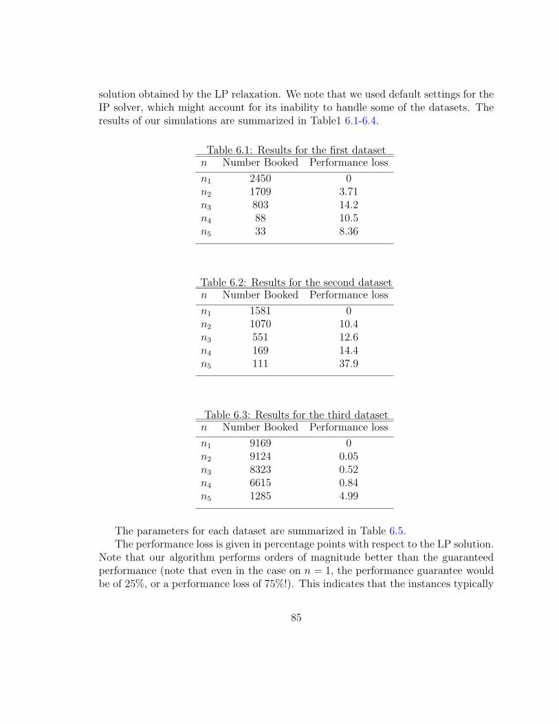
solution obtained by the LP relaxation. We note that we used default settings for theIP solver, which might account for its inability to handle some of the datasets. Theresults of our simulations are summarized in Table1 6.1-6.4.

Table 6.1: Results for the first datasetn Number Booked Performance loss

n1 2450 0n2 1709 3.71n3 803 14.2n4 88 10.5n5 33 8.36

Table 6.2: Results for the second datasetn Number Booked Performance loss

n1 1581 0n2 1070 10.4n3 551 12.6n4 169 14.4n5 111 37.9

Table 6.3: Results for the third datasetn Number Booked Performance loss

n1 9169 0n2 9124 0.05n3 8323 0.52n4 6615 0.84n5 1285 4.99

The parameters for each dataset are summarized in Table 6.5.The performance loss is given in percentage points with respect to the LP solution.

Note that our algorithm performs orders of magnitude better than the guaranteedperformance (note that even in the case on n = 1, the performance guarantee wouldbe of 25%, or a performance loss of 75%!). This indicates that the instances typically

85

Table 6.4: Results for the fourth datasetn Number Booked Performance loss

n1 8826 0n2 6355 20.0n3 4603 23.6n4 850 8.09n5 436 6.72

Table 6.5: Parameters of the datasetsParameters Dataset1 Dataset2 Dataset3 Dataset4

n1 5M 5M 1B 500Mn2 1M 1M 500M 100Mn3 500k 500k 100M 50Mn4 100k 100k 50M 10Mn5 50k 50k 10M 5M

# contracts 2450 1581 9169 8826T 12 90 90 90

encountered in real setting are far from those necessary to make our algorithm performpoorly.

In Table 6.6 we compare the performance of the IP solution to that of the LPsolution. Note that for datasets two to four, the performance of the integer pro-gramming solution was sometimes below that of our solution, and in some instanceswas not even available. We used the open source branch and cut code Cbc from theCOIN-OR repository [41], with default parameter settings, but with the attemptedaddition of the probing, Gomory, knapsack, redsplit and clique cuts. In general, thenumber of cuts obtained was small. The branch and bound algorithm was run untileither the 10th integer solution was obtained, or twenty minutes have elapsed.

86

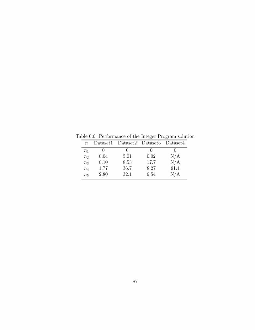
Table 6.6: Performance of the Integer Program solution

n Dataset1 Dataset2 Dataset3 Dataset4

n1 0 0 0 0n2 0.04 5.01 0.02 N/An3 0.10 8.53 17.7 N/An4 1.77 36.7 8.27 91.1n5 2.80 32.1 9.54 N/A

87

Chapter 7Conclusion and Future Work

Online advertising is an emerging field in computer science and it is also the mainrevenue resource for large search engine companies. In this thesis, we focused ononline advertising and described different ways of online advertising. We consideredsome problems related to this way of advertising and suggested some solutions. Weconclude this thesis by describing the summary of our results and some of the futuredirections to pursue research in this area. We looked at four main problems relatedto online advertising and presented the solution to each problem. In these problems,we considered constraints that are forced by the real system requirements such asspace(memory) constraint, speed and simplicity, and the same time we tried to max-imize objective functions defined for each problem. In Non Guaranteed Delivery welooked at two problems.

• Online Ad Allocation Problem

• Query Rewriting Problem

We start by generalizing the notion of Submodularity over set functions to a morebroad class of functions (i.e., Sequence Functions) and showed that the result ofNemhauser et al [46] still holds for Sequence Submodular functions. As we saw inthis thesis, this result is useful in analyzing the performance of a greedy approach foronline problems. We used this property as a tool to analyze Online Ad Allocationproblem as well as the weighted version of Query Rewriting problem. We showedthat if the queries are coming from a fixed but unknown distribution during time, thegreedy approach obtains at least (1− 1

e) of the profit in expectation. This is a good

news since greedy algorithms are simple and fast and this result shows that theirprofit is also good. The second problem that we considered was the query rewritingproblem. Query rewriting was used in Yahoo! as a tool to help retrieving relevant ads.However, the original design was only based on the relevance of the original queryto the rewrites (similar to the ones for information retrieval) and new requirementsfor advertisement was not included. We considered this problem from the advertisingpoint of view, defined a new set of constraints and objectives and then developeda solution based on this new model. Also, for the first time, we modeled a globalvariant of the problem by considering all queries together and defined the appropriateconstraints and requirements for the global variant. We considered two models:

88

Cardinality Version: In this variant, the constraints specify upper bounds on boththe number of rewrites a query can have as well as the number of queries forwhich a query rewrite can be used. These model the system constraints inan ad network: too many rewrites for a given query will slow down the timeneeded to serve an ad and using the same rewrite for too many queries will makethe ads less diverse. For this model, we proposed a greedy algorithm with anapproximation ratio of (e− 1)/(2e− 1) ≈ 0.387. This ratio is an improvementover 1/3 that can be obtained using existing results on greedy algorithms formatroid intersections; we believe this may be of independent interest.

Weighted Version: In the second variant (called the weighted version), we modeledthe constraints of an ad’s budget. We assumed that the traffic for a query for afixed period of time is known. The goal here was again to select a set of rewritesthat have the maximum benefit subject to the constraint that no query canhave too many rewrites. The key difference was that an ad can only contributebenefit for traffic up to its budget. For this version, we proposed another greedyalgorithm with an approximation ratio of 1− 1

e1−1e. In the analysis, we used the

sequence submodularity property.

Research on Guaranteed Delivery Advertisement is getting more popular. In this cate-gory as we mentioned before, advertisers are more interested in branding. As a result,they need their ad to be shown to a good set of users that are related to advertisersdesired set of keywords. As a result, they want that the search engine guarantees toallocate their required number of impressions to them for their requested time period.Two main questions in this area are: (a) to decide which set of advertisers to acceptand sign a contract with. (b) after accepting a set of advertisers as contractors, whichallocation is the most favorable one for contractors. We looked at the following twoproblems:

Online Ad Allocation for Display Advertisement The model we considered isas follows: Advertisers arrive online and request a contract. Upon arrival,advertiser k reveals all her information including the number of impressionsshe is interested per day and the start and the end of the time period thatshe wants her ads to be displayed. We assumed that the payment is accordingto the total number of impressions that will be allocated to an advertiser (ifand only if her total demand will be satisfied). The publisher then decideson the spot to accept or reject the contract. We also assume that the totalnumber of available impressions per day is fixed. Contracts can be droppedwithout penalty (i.e., the publisher can accept a contract and drop it later if a

89

better one arrives). However in this case publisher cannot charge the advertiseranything if the contract is dropped. The goal is to maximize social welfare (orrevenue) under adversarial arrival of advertisers. Under these assumptions, weshowed that for an arbitrary sequence of advertisers, there is no online algorithmthat can have a worst case ratio smaller than n where n is the total number ofavailable impressions per day. We then presented an online greedy algorithmwith a worst case analysis and we showed that the obtained profit from ouralgorithm is only a constant factor worse than the best possible online algorithm.Since the lower bound on the best possible algorithm in the adversary settingis quite pessimistic, we simulated the performance of our greedy algorithm onactual data from Yahoo!’s display advertisement business. We found that ouralgorithm performs very well in practice as the observed performance was quiteclose to the optimal, as opposed to the worst case lower bound.

Fair Contract Allocation Given a set of impressions (i.e., the supply) and thenumber of available impressions and contracts with their desired number of im-pressions, how to find a feasible assignment of impressions to contracts that isas fair as possible? Answering this question involves formulating what fairnessprecisely means in this context. And, given the large number of advertisers(typically, in the hundreds of thousands) and the astronomical number of im-pressions (typically, in the hundreds of millions) in an online setting, we desirean allocation algorithm that is practical and combinatorial and whose allocationcan be stored succinctly, ideally, using space linear in the number of impres-sions and contracts as opposed to the naive quadratic storage. Of course, thissuccinct representation should let us reconstruct the allocation along every pairof contract and impression bucket in a time-efficient manner. The price of eachimpression is computed based on the historical data. We considered the generalproblem of fair allocation in a bipartite supply-demand setting. Our formu-lation is combinatorial and captures the notion of deviation from fairness bya natural and general form of a penalty function. For the case of L1 penaltyfunctions we obtained a simple combinatorial algorithm for the fair allocationproblem. By L1 penalty function, we mean that we want to find a feasible al-location of impressions to contracts while minimizing the absolute distance ofthis allocation from the most representative allocation for each contract. Oursolution was based on solving a min-cost flow problem on a bipartite graph,which has been done very efficiently. We also showed how to precompute andstore a linear amount of information such that the allocation along any edgein the bipartite graph can be approximately answered in constant time, under

90

mild assumptions on the input instances. This space-efficient reconstructionmethod might be of independent interest in contexts beyond fair allocation.

We also proved two additional properties of our formulation. First is robustness,where we show how to upper bound the performance loss when the supply esti-mates are only approximately known. Second is extensibility, where we showedan even simpler greedy approximation algorithm when some of the demandconstraints are relaxed.

Finally, we extended our combinatorial solution to any convex function.

7.1 Future Work

In the context of online algorithms, one approach is to design algorithms witha good worst case performance. Another approach is to design an algorithm withgood expected performance. As we saw, in the context of online ad allocation inNon-Guaranteed Delivery, by adding the assumption that the queries are comingfrom an unknown distribution, we can get a better approximation factor. Computerscientists have traditionally adopted the former approach since it does not dependon the probability distribution of the input and worst case analysis is generally muchsimpler than analysis of the expected performance. Nevertheless, many algorithmswith theoretically not so good worst case performance do much better in practicesince they have a better performance in expectation.

The offline version of many online algorithms like online resource allocation [14],use linear programming to find an intermediate fractional solution. A similar LPapproach usually cannot be used for the online version since solving the LP requiresall the information to be known in advance. Still it might be possible to find certainforms of LP’s for which an approximation to the optimal solution can be constructedgradually. Consider for example the following class of linear programs:

Definition 1 (Online Packing LP:). Consider the linear program of the followingform:

maximize: c.x (7.1.1)

Ax ≤ b (7.1.2)

xi ∈ [0, 1] (7.1.3)

such that the matrix A and the vectors b and c are non-negative. We say each variablexi, has the status of being active or inactive. If inactive then xi = 0 otherwise xicould take any value in [0, 1]. We learn the status (i.e., active/inactive) of variable

91

xi at time ti and as soon as we find out its status we are required to choose its value(if inactive it should be set to 0). Once initialized, the value of a variable cannot bechanged at a later time. As for distribution information, we know that each variablexi will be active with probability pi independent of other variables. The goal is todesign an online algorithm that would maximize the expected value of the objectivefunction.

The online resource allocation problem [14] can be easily modeled as an onlinepacking LP. If we could efficiently compute the expected value of the objective func-tion for the optimal offline solver then we could use the following online algorithm.At each time ti that the status of variable xi is revealed, if xi is active then computethe expected value of the objective for the rest of the LP once for xi = 0 and once forxi = 1 and the choose then one with the highest total expected value. Therefore, itis interesting to see if there is an efficient way to compute the expected value of theobjective function. It is worth mentioning that we can efficiently compute an upperbound on the expected value of the objective by adding the constraints xi ≤ pi andsolve the offline linear program. It might also be possible to compute an approxi-mation to the optimal online algorithm if we could compute a constant factor lowerbound for the expected value of the objective function and then use that instead ofthe exact expected value in the online algorithm. This problem will cover a lot ofother problems assuming that the inputs are coming from a distribution (e.g., OnlineAd Allocation in Guaranteed Delivery).

Another open problem is related to the online ad allocation problem in Non-Guaranteed Delivery from the game theoretic perspective. In the current setting weassumed that we know the payments of each ad for each keyword. However in reality,advertisers are bidding on each keyword and the payment is computed based on thebids of the participants in the auction. Assuming that bidders are strategic it is notthe case that they will bid their true valuation for each keyword. The interestingquestion arises when we consider the budget constraint as well. The new problem canbe summarized as follows:

• Assuming that the advertisers are strategic and rational and assuming that theyhave a budget constraint that is publicly known, design a mechanism that willmaximize the revenue of the search engine.

We can consider Fair Allocation Problem from game theoretic aspect as well. Thequestion can be defined as follows:

• Suppose again that advertisers are rational and strategic. Design a pricingstrategy so that assuming that we use the allocation described in chapter 5,truth telling about the demand is dominant strategy for advertisers.

92

To conclude, I believe that the problems in this thesis address a few of the currentchallenges in e-Commerce and Internet Advertising. There are many interesting newproblems arising in this field and the area is rapidly growing. I believe that this isone of the areas that will receive higher attention for research in the near future dueto its potential for generating revenue at large scales for IT companies.

93

Bibliography

[1] A. Agrawal, P. N. Klein, and R. Ravi. When trees collide: An approximationalgorithm for the generalized Steiner problem on networks. In Proc. 23rd AnnualACM Symposium on Theory of Computing, pages 134–144, 1991.

[2] R. K. Ahuja, T. L. Magnanti, and J. B. Orlin. Network Flows: Theory, Algo-rithms and Applications. Prentice Hall, 1993.

[3] S. Alaei, E. Arcaute, S. Khuller, W. Ma, A. Malekian, and J. Tomlin. Onlineallocation of display advertisements subject to advanced sales contracts. In KDDWorkshop on Data Mining and Audience Intelligence for Advertising, pages 69–77, 2009.

[4] S. Alaei, R. Kumar, A. Malekian, and E. Vee. Fair allocation with succintrepresentation, 2009.

[5] S. Alaei and A. Malekian. Maximizing sequence-submodular functions and itsapplication to online advertising, 2008.

[6] N. Andelman and Y. Mansour. Auctions with budget constraints. In 9th Scan-dinavian Workshop on Algorithm Theory (SWAT), pages 26–38, 2004.

[7] I. Antonellis, H. G. Molina, and C.-C. Chang. Simrank++: Query rewritingthrough link analysis of the click graph. In Stanford Computer Science Depart-ment Technical Report, 2007.

[8] Y. Azar, B. Birnbaum, A. R. Karlin, C. Mathieu, and C. T. Nguyen. Improvedapproximation algorithms for budgeted allocations. In ICALP ’08: Proceedingsof the 35th international colloquium on Automata, Languages and Programming,Part I, pages 186–197, 2008.

[9] M. Babaioff, J. Hartline, and R. Kleinberg. Selling banner ads: Online algorithmswith buyback. In Proc. 4th Workshop on Ad Auctions, 2008.

[10] R. Bar-Yehuda and S. Even. A linear-time approximation algorithm for theweighted vertex cover problem. J. Algorithms, 2(2):198–203, 1981.

[11] D. Beeferman and A. Berger. Agglomerative clustering of a search engine querylog. In Proc. 6th KDD, pages 407–416, 2000.

94

[12] J. Breese, D. Heckerman, and C. Kadie. Empirical analysis of predictive algo-rithms for collaborative filtering. In In Proc. 14th UAI, pages 43–52, 1998.

[13] A. L. Buchsbaum, H. J. Karloff, C. Kenyon, N. Reingold, and M. Thorup. Optversus load in dynamic storage allocation. SIAM J. Comput., 33(3):632–646,2004.

[14] G. Calinescu, A. Chakrabarti, H. J. Karloff, and Y. Rabani. Improved approxi-mation algorithms for resource allocation. In Proceedings of the 9th InternationalInteger Programming and Combinatorial Optimization Conference, IPCO 2002,pages 401–414, 2002.

[15] D. Chakrabarty and G. Goel. On the approximability of budgeted allocations andimproved lower bounds for submodular welfare maximization and gap. In FOCS’08: Proceedings of the 2008 49th Annual IEEE Symposium on Foundations ofComputer Science, pages 687–696, Washington, DC, USA, 2008.

[16] F. Constantin, J. Feldman, S. Muthukrishnan, and M. Pl. An online mechanismfor ad slot reservations with cancellations. In SODA, 2009.

[17] S. C. Deerwester, S. T. Dumais, T. K. Lancaster, G. W. Furnas, and R. Harsh-man. Indexing by latent semantic analysis. In JASIS, pages 391–407, 1990.

[18] N. R. Devanur and T. P. Hayes. The adwords problem: online keyword matchingwith budgeted bidders under random permutations. In EC ’09: Proceedings ofthe tenth ACM conference on Electronic commerce, pages 71–78, New York, NY,USA, 2009. ACM.

[19] N. R. Devanur, C. H. Papadimitriou, A. Saberi, and V. V. Vazirani. Marketequilibrium via a primal-dual algorithm for a convex program. J. ACM, 55(5),2008.

[20] B. Edelman, M. Ostrovsky, and M. Schwarz. Internet advertising and the general-ized second price auction: Selling billions of dollars worth of keywords. AmericanEconomic Review, 97(1):242–259, 2007.

[21] L. Epstein and A. Levin. Improved randomized results for that interval selectionproblem. In ESA, pages 381–392, 2008.

[22] U. Feige, N. Immorlica, V. S. Mirrokni, and H. Nazerzadeh. A combinatorialallocation mechanism with penalties for banner advertising. In WWW, pages169–178, 2008.

95

[23] U. Feige, V. S. Mirrokni, and J. Vondrak. Maximizing non-monotone submodularfunctions. In FOCS ’07: Proceedings of the 48th Annual IEEE Symposium onFoundations of Computer Science, pages 461–471, Washington, DC, USA, 2007.IEEE Computer Society.

[24] L. Fleischer, M. X. Goemans, V. S. Mirrokni, and M. Sviridenko. Tight ap-proximation algorithms for maximum general assignment problems. In SODA’06: Proceedings of the seventeenth annual ACM-SIAM symposium on Discretealgorithm, pages 611–620, New York, NY, USA, 2006. ACM.

[25] R. Garg, V. Pandit, and V. Kumar. Approximation algorithms for budget-constrained auctions, 2001.

[26] A. Ghosh, P. McAfee, K. Papineni, and S. Vassilvitskii. Bidding for representa-tive allocations for display advertising, 2009.

[27] G. Goel and A. Mehta. Online budgeted matching in random input models withapplications to adwords. In SODA ’08: Proceedings of the nineteenth annualACM-SIAM symposium on Discrete algorithms, pages 982–991, Philadelphia,PA, USA, 2008. Society for Industrial and Applied Mathematics.

[28] A. V. Goldberg and R. E. Tarjan. A new approach to the maximum-flow problem.J. ACM, 35(4):921–940, 1988.

[29] P. Goundan and A. Schulz. Revisiting the greedy approach to submodular setfunction maximization. In Manuscript, 2007.

[30] J. Herlocker, J. Konstan, A. Borchers, and J. Riedl. An algorithmic frameworkfor performing collaborative filtering. In Proc. 22nd SIGIR, pages 230–237, 1999.

[31] S. Iwata, L. Fleischer, and S. Fujishige. A combinatorial, strongly polynomial-time algorithm for minimizing submodular functions. Journal of the ACM,48:761–777, 2001.

[32] S. IWATA, L. FLEISCHER, I. Lisa, and S. FUJISHIGE. A combinatorialstrongly polynomial algorithm for minimizing submodular functions. Journalof the ACM, 48:761–777, 2000.

[33] K. Jain and V. V. Vazirani. Eisenberg-Gale markets: Algorithms and structuralproperties. In Proc. 39th Annual ACM Symposium on Theory of Computing,pages 364–373, 2007.

96

[34] G. Jeh and J. Widom. Simrank: A measure of structural-context similarity. InProc. 8th KDD, pages 538–543, 2002.

[35] R. Jones, B. Rey, O. Madani, and W. Greiner. Generating query substitutions.In Proc. 15th WWW, pages 387–396, 2006.

[36] R. M. Karp, U. V. Vazirani, and V. V. Vazirani. An optimal algorithm for on-line bipartite matching. In STOC ’90: Proceedings of the twenty-second annualACM symposium on Theory of computing, pages 352–358, New York, NY, USA,1990. ACM.

[37] S. Khot, R. J. Lipton, E. Markakis, and A. Mehta. Inapproximability resultsfor combinatorial auctions with submodular utility functions. In WINE, pages92–101, 2005.

[38] S. Khuller, A. Moss, and J. S. Naor. The budgeted maximum coverage problem.Inf. Process. Lett., 70(1):39–45, 1999.

[39] B. Lehmann, D. Lehmann, and N. Nisan. Combinatorial auctions with decreasingmarginal utilities. Games and Economic Behavior, 55(2):270–296, May 2006.

[40] A. Malekian, C.-C. Chang, R. Kumar, and G. Wang. Optimizing query rewritesfor keyword-based advertising. In EC ’08: Proceedings of the 9th ACM conferenceon Electronic commerce, pages 10–19, New York, NY, USA, 2008. ACM.

[41] COIN-OR Foundation: http://www.coin or.org.

[42] P. McAfee and K. Papineni. Maximally representative allocation for guaranteeddelivery advertising campaigns, 2008. Manuscript.

[43] A. Mehta, A. Saberi, U. Vazirani, and V. Vazirani. Adwords and generalizedonline matching. J. ACM, 54(5):22, 2007.

[44] H. Miyazawa and T. Erlebach. An improved randomized on-line algorithm for aweighted interval selection problem. J. Scheduling, 7(4):293–311, 2004.

[45] G. L. Nemhauser and L. A. Wolsey. Best algorithms for approximating themaximum of a submodular set function. Mathematics of Operations Research,3(3):177–188, 1978.

[46] G. L. Nemhauser, L. A. Wolsey, and M. L. Fisher. An analysis of approximationsfor maximizing submodular set functions. volume 14, pages 265–294, Berlin,Heidelberg, 1978. Springer.

97

[47] G. L. Nemhauser, L. A. Wolsey, and M. L. Fisher. An analysis of approximationsfor maximizing submodular set functions. In Math. Prog., pages 265–294, 1978.

[48] S. S. Seiden. Randomized online interval scheduling. Oper. Res. Lett., 22(4-5):171–177, 1998.

[49] A. Srinivasan. Budgeted allocations in the full-information setting. In APPROX-RANDOM, pages 247–253, 2008.

[50] E. Vee, S. Vassilvitskii, and J. Shanmugasundaram. Online allocation with acompact plan, 2009. yahoo research reoport, YL-2009-05.

[51] G. J. Woeinger. On-line scheduling of jobs with fixed start and end times.Theoretical Computer Science, 130(1):5–16, 1994.

[52] W. Zhang and R. Jones. Comparing click logs and editorial labels for trainingquery rewriting. In Workshop on Query Log Analysis, 16th WWW, 2007.

[53] W. V. Zhang, X. H. Fei, B. Rey, and R. Jones. Query rewriting using activelearning for sponsored search. In Proc. 30th SIGIR, pages 853–854, 2007.

98