Synthesizing the preferred inputs for neurons inneural networks via deep generator networks

Anh Nguyenanguyen8@uwyo.edu

Alexey Dosovitskiydosovits@cs.uni-freiburg.de

Jason Yosinskijason@geometricintelligence.com

Thomas Broxbrox@cs.uni-freiburg.de

Jeff Clunejeffclune@uwyo.edu

Abstract

Deep neural networks (DNNs) have demonstrated state-of-the-art results on manypattern recognition tasks, especially vision classification problems. Understandingthe inner workings of such computational brains is both fascinating basic sciencethat is interesting in its own right—similar to why we study the human brain—andwill enable researchers to further improve DNNs. One path to understandinghow a neural network functions internally is to study what each of its neuronshas learned to detect. One such method is called activation maximization (AM),which synthesizes an input (e.g. an image) that highly activates a neuron. Herewe dramatically improve the qualitative state of the art of activation maximizationby harnessing a powerful, learned prior: a deep generator network (DGN). Thealgorithm (1) generates qualitatively state-of-the-art synthetic images that lookalmost real, (2) reveals the features learned by each neuron in an interpretableway, (3) generalizes well to new datasets and somewhat well to different networkarchitectures without requiring the prior to be relearned, and (4) can be consideredas a high-quality generative method (in this case, by generating novel, creative,interesting, recognizable images).

1 Introduction and Related Work

Understanding how the human brain works has been a long-standing quest in human history. Neuro-scientists have discovered neurons in human brains that selectively fire in response to specific, abstractconcepts such as Halle Berry or Bill Clinton, shedding light on the question of whether learned neuralcodes are local vs. distributed [1]. These neurons were identified by finding the preferred stimuli(here, images) that highly excite a specific neuron, which was accomplished by showing subjectsmany different images while recording a target neuron’s activation. Such neurons are multifaceted:for example, the “Halle Berry neuron” responds to very different stimuli related to the actress—frompictures of her face, to pictures of her in costume, to the word “Halle Berry” printed as text [1].

Inspired by such neuroscience research, we are interested in shedding light into the inner workingsof DNNs by finding the preferred inputs for each of their neurons. As the neuroscientists did, onecould simply show the network a large set of images and record a set of images that highly activate aneuron [2]. However, that method has disadvantages vs. synthesizing preferred stimuli: 1) it requiresa distribution of images that are similar to those used to train the network, which may not be known(e.g. when probing a trained network when one does not know which data were used to train it); 2)

29th Conference on Neural Information Processing Systems (NIPS 2016), Barcelona, Spain.

arX

iv:1

605.

0930

4v1

[cs

.NE

] 3

0 M

ay 2

016

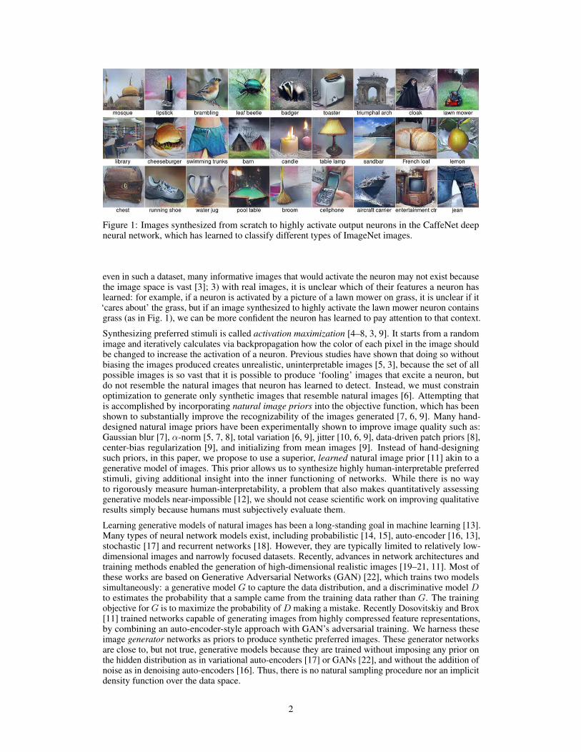
Figure 1: Images synthesized from scratch to highly activate output neurons in the CaffeNet deepneural network, which has learned to classify different types of ImageNet images.

even in such a dataset, many informative images that would activate the neuron may not exist becausethe image space is vast [3]; 3) with real images, it is unclear which of their features a neuron haslearned: for example, if a neuron is activated by a picture of a lawn mower on grass, it is unclear if it‘cares about’ the grass, but if an image synthesized to highly activate the lawn mower neuron containsgrass (as in Fig. 1), we can be more confident the neuron has learned to pay attention to that context.

Synthesizing preferred stimuli is called activation maximization [4–8, 3, 9]. It starts from a randomimage and iteratively calculates via backpropagation how the color of each pixel in the image shouldbe changed to increase the activation of a neuron. Previous studies have shown that doing so withoutbiasing the images produced creates unrealistic, uninterpretable images [5, 3], because the set of allpossible images is so vast that it is possible to produce ‘fooling’ images that excite a neuron, butdo not resemble the natural images that neuron has learned to detect. Instead, we must constrainoptimization to generate only synthetic images that resemble natural images [6]. Attempting thatis accomplished by incorporating natural image priors into the objective function, which has beenshown to substantially improve the recognizability of the images generated [7, 6, 9]. Many hand-designed natural image priors have been experimentally shown to improve image quality such as:Gaussian blur [7], α-norm [5, 7, 8], total variation [6, 9], jitter [10, 6, 9], data-driven patch priors [8],center-bias regularization [9], and initializing from mean images [9]. Instead of hand-designingsuch priors, in this paper, we propose to use a superior, learned natural image prior [11] akin to agenerative model of images. This prior allows us to synthesize highly human-interpretable preferredstimuli, giving additional insight into the inner functioning of networks. While there is no wayto rigorously measure human-interpretability, a problem that also makes quantitatively assessinggenerative models near-impossible [12], we should not cease scientific work on improving qualitativeresults simply because humans must subjectively evaluate them.

Learning generative models of natural images has been a long-standing goal in machine learning [13].Many types of neural network models exist, including probabilistic [14, 15], auto-encoder [16, 13],stochastic [17] and recurrent networks [18]. However, they are typically limited to relatively low-dimensional images and narrowly focused datasets. Recently, advances in network architectures andtraining methods enabled the generation of high-dimensional realistic images [19–21, 11]. Most ofthese works are based on Generative Adversarial Networks (GAN) [22], which trains two modelssimultaneously: a generative model G to capture the data distribution, and a discriminative model Dto estimates the probability that a sample came from the training data rather than G. The trainingobjective forG is to maximize the probability ofD making a mistake. Recently Dosovitskiy and Brox[11] trained networks capable of generating images from highly compressed feature representations,by combining an auto-encoder-style approach with GAN’s adversarial training. We harness theseimage generator networks as priors to produce synthetic preferred images. These generator networksare close to, but not true, generative models because they are trained without imposing any prior onthe hidden distribution as in variational auto-encoders [17] or GANs [22], and without the addition ofnoise as in denoising auto-encoders [16]. Thus, there is no natural sampling procedure nor an implicitdensity function over the data space.

2

...

I m age

banana

convertible..

...

Deep   generator  network(prior) DNN   being  visualized

candle

CodeForward  and  backward  passes

u9 u2u1 c1

c2

fc6 fc7fc8fc6

c3 c4 c5. . .

up c o n v o l u t i o n a l c o n v o l u t i o n a l

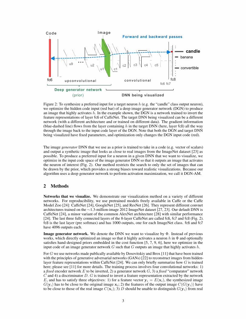
Figure 2: To synthesize a preferred input for a target neuron h (e.g. the “candle” class output neuron),we optimize the hidden code input (red bar) of a deep image generator network (DGN) to producean image that highly activates h. In the example shown, the DGN is a network trained to invert thefeature representations of layer fc6 of CaffeNet. The target DNN being visualized can be a differentnetwork (with a different architecture and or trained on different data). The gradient information(blue-dashed line) flows from the layer containing h in the target DNN (here, layer fc8) all the waythrough the image back to the input code layer of the DGN. Note that both the DGN and target DNNbeing visualized have fixed parameters, and optimization only changes the DGN input code (red).

The image generator DNN that we use as a prior is trained to take in a code (e.g. vector of scalars)and output a synthetic image that looks as close to real images from the ImageNet dataset [23] aspossible. To produce a preferred input for a neuron in a given DNN that we want to visualize, weoptimize in the input code space of the image generator DNN so that it outputs an image that activatesthe neuron of interest (Fig. 2). Our method restricts the search to only the set of images that canbe drawn by the prior, which provides a strong biases toward realistic visualizations. Because ouralgorithm uses a deep generator network to perform activation maximization, we call it DGN-AM.

2 Methods

Networks that we visualize. We demonstrate our visualization method on a variety of differentnetworks. For reproducibility, we use pretrained models freely available in Caffe or the CaffeModel Zoo [24]: CaffeNet [24], GoogleNet [25], and ResNet [26]. They represent different convnetarchitectures trained on the ∼1.3-million-image 2012 ImageNet dataset [27, 23]. Our default DNN isCaffeNet [24], a minor variant of the common AlexNet architecture [28] with similar performance[24]. The last three fully connected layers of the 8-layer CaffeNet are called fc6, fc7 and fc8 (Fig. 2).fc8 is the last layer (pre softmax) and has 1000 outputs, one for each ImageNet class. fc6 and fc7have 4096 outputs each.

Image generator network. We denote the DNN we want to visualize by Φ. Instead of previousworks, which directly optimized an image so that it highly activates a neuron h in Φ and optionallysatisfies hand-designed priors embedded in the cost function [5, 7, 9, 6], here we optimize in theinput code of an image generator network G such that G outputs an image that highly activates h.

ForG we use networks made publically available by Dosovitskiy and Brox [11] that have been trainedwith the principles of generative adversarial networks (GANs) [22] to reconstruct images from hidden-layer feature representations within CaffeNet [24]. We can only briefly summarize how G is trainedhere; please see [11] for more details. The training process involves four convolutional networks: 1)a fixed encoder network E to be inverted, 2) a generator network G, 3) a fixed “comparator” networkC and 4) a discriminator D. G is trained to invert a feature representation extracted by the networkE, and has to satisfy three objectives: 1) for a feature vector yi = E(xi), the synthesized imageG(yi) has to be close to the original image xi; 2) the features of the output image C(G(yi)) haveto be close to those of the real image C(xi); 3) D should be unable to distinguish G(yi) from real

3

images. The objective for D is to discriminate between synthetic images G(yi) and real images xi

as in the original GAN [22].

In this paper, the encoder E is CaffeNet truncated at different layers. We denote CaffeNet truncatedat layer l by El, and the network trained to invert El by Gl. The “comparator” C is CaffeNet up tolayer pool5. D is a convolutional network with 5 convolutional and 2 fully connected layers. G is anupconvolutional (aka deconvolutional) architecture [19] with 9 upconvolutional and 3 fully connectedlayers. Detailed architectures are provided in [11].

Synthesizing the preferred images for a neuron. Intuitively, we search in the input code spaceof the image generator model G to find a code y such that G(y) is an image that produces highactivation of the target neuron h in the DNN Φ that we want to visualize (i.e. optimization maximizesΦh(G(y))). Recall that Gl is a generator network trained to reconstruct images from the l-th layerfeatures of CaffeNet. Formally, and including a regularization term, we may pose the activationmaximization problem as finding a code yl such that:

yl = arg maxyl

(Φh(Gl(yl))− λ‖yl‖) (1)

Empirically, we found a small amount of L2 regularization (λ = 0.005) works best. We also computethe activation range for each neuron in the set of codes {yl

i} computed by running validation setimages through El. We then clip each neuron in yl to be within the activation range of [0, 3σ], whereσ is one standard deviation around the mean activation (the activation is lower bounded at 0 due tothe ReLU nonlinearities that exist at the layers whose codes we optimize). This clipping acts as aprimitive prior on the code space and substantially improves the image quality. In future work, weplan to learn this prior via a GAN or other generative model.

Because the true goal of activation maximization is to generate interpretable preferred stimuli foreach neuron, we performed random search in the hyperparameter space consisting of L2 weight λ,number of iterations, and learning rate. We chose the hyperparameter settings that produced thehighest quality images. We note that we found no correlation between the activation of a neuron andthe recognizability of its visualization.

3 Results

3.1 Comparison between priors trained to invert features from different layers

Since a generator model Gl could be trained to invert feature representations of an arbitrary layer l ofE, we sampled l = {3, 5, 6, 7} to explore the impact on this choice and identify qualitatively whichproduces the best images. Here, the DNN to visualize Φ is the same as the encoder E (CaffeNet), butthey can be different (as shown below). The Gl networks are from [11]. For each Gl network wechose the hyperparameter settings from a random sample that gave the best qualitative results.

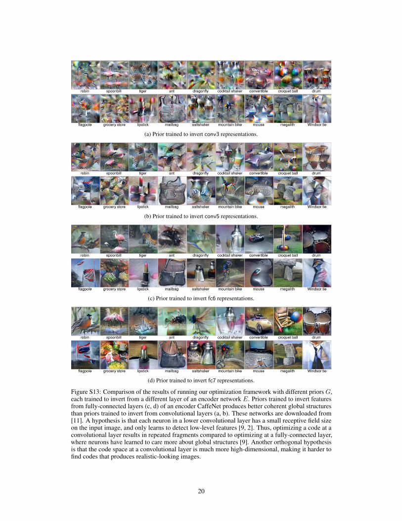
Optimizing codes from the convolutional layers (l = 3, 5) typically yields highly repeated fragments,whereas optimizing fully-connected layer codes produces much more coherent global structure(Fig. S13). Interestingly, previous studies have shown that G trained to invert lower-layer codes(smaller l) results in far better reconstructions than higher-layer codes [29, 6]. That can be explainedbecause those low-level codes come from natural images, and contain more information aboutimage details than more abstract, high-level codes. For activation maximization, however, we aresynthesizing an entire layer code from scratch. We hypothesize that this process works worse forGl priors with smaller l because each feature in low-level codes has a small, local receptive field.Optimization thus has to independently tune features throughout the image without knowing theglobal structure. For example, is it an image of one or four robins? Because fully-connected layershave information from all areas of the image, they represent information such as the number, location,size, etc. of an object, and thus all the pixels can be optimized toward this agreed upon structure. Anorthogonal, non-mutually-exclusive hypothesis is that the code space at a convolutional layer is muchmore high-dimensional, making it harder to optimize.

We found that optimizing in the fc6 code space produces the best visualizations (Figs. 1 & S13). Wethus use this G6 DGN as the default prior for the experiments in the rest of the paper. In addition,our images qualitatively appear to be the most realistic-looking compared to visualizations from all

4

previous methods (Fig. S17). Our result reveals that a great amount of fine detail and global structureare captured by the DNN even at the last output layer.

This finding is in contrast to a previous hypothesis that DNNs trained with supervised learning oftenignore an object’s global structure, and only learn discriminative features per class (e.g. color ortexture) [3]. Section 3.5 provides evidence that this global structure does not come from the prior.

To test whether our method memorizes the training set images, we retrieved the closest images fromthe training set for each of sample synthetic images. Specifically, for each synthetic image for anoutput neuron Y (e.g. lipstick), we find an image among the same class Y with the lowest Euclideandistance in pixel space, as done in previous works [22], but also in each of the 8 code spaces of theencoder DNN. While this is a much harder test than comparing to a nearest neighbor found among theentire dataset, we found no evidence that our method memorizes the training set images (Fig. S22).We believe evaluating similarity in the code spaces of deep representations, which better capturesemantic aspects of images, is a more informative approach compared to evaluating only in the pixelspace.

3.2 Does the learned prior trained on ImageNet generalize to other datasets?

We test whether the same DNN prior (G6) that was trained on inverting the feature representations ofImageNet images generalizes to enable visualizing DNNs trained on different datasets. Specifically,we target the output neurons of two DNNs downloaded from Caffe Model Zoo [24]): (1) An AlexNetDNN that was trained on the 2.5-million-image MIT Places dataset to classify 205 types of placeswith 50.1% accuracy [30]. (2) A hybrid architecture of CaffeNet and the network in [2] createdby [31] to classify actions in videos by processing each frame of the video separately. The datasetconsists of 13,320 videos categorized into 101 human action classes.

For DNN 1, the prior trained on ImageNet images generalizes well to the completely different MITPlaces dataset (Fig. 3). This result suggests the prior trained on ImageNet will generalize to othernatural image datasets, at least if the architecture of the DNN to be visualized Φ is the same asthe architecture of the encoder network E from which the generator model G was trained to invertfeature representations. For DNN 2: the prior generalizes to produce decent results; however, theimages are not qualitatively as sharp and clear as for DNN 1 (Fig. 4). We have two orthogonalhypotheses for why this happens: 1) Φ (the DNN from [31]) is a heavily modified version of E(CaffeNet); 2) the two types of images are too different: the primarily object-centric ImageNet datasetvs. the UCF-101 dataset, which focuses on humans performing actions. Sec. 3.3 returns to the firsthypothesis regarding how the similarity between Φ and E affects the image quality

Overall, the prior trained with a CaffeNet encoder generalizes well to visualizing other DNNs of thesame CaffeNet architecture trained on different datasets.

Figure 3: Preferred stimuli for output units of an AlexNet DNN trained on the MIT Places dataset [30],showing that the ImageNet-trained prior generalizes well to a dataset comprised of images of scenes.

5

Figure 4: Preferred images for output units of a heavily modified version of the AlexNet architecturetrained to classify videos into 101 classes of human activities [31]. Here, we optimize a singlepreferred image per neuron because the DNN only classifies single frames (whole video classificationis done by averaging scores across all video frames).

3.3 Does the learned prior generalize to visualizing different architectures?

We have shown that when the DNN to be visualized Φ is the same as the encoder E, the resultantvisualizations are quite realistic and recognizable (Sec. 3.1). To visualize a different networkarchitecture Φ, one could train a new G to invert Φ feature representations. However, training a newG DGN for every DNN we want to visualize is computationally costly. Here, we test whether thesame DGN prior trained on CaffeNet (G6) can be used to visualize two state-of-the-art DNNs that arearchitecturally different from CaffeNet, but were trained on the same ImageNet dataset. Both weredownloaded from Caffe Model Zoo and have similar accuracy scores: (a) GoogLeNet is a 22-layernetwork and has a top-5 accuracy of 88.9% [25]; (b) ResNet is a new type of very deep architecturewith skip connections [26]. We visualize a 50-layer ResNet that has a top-5 accuracy of 93.3%. [26].

DGN-AM produces the best image quality when Φ = E, and the visualization quality tends todegrade as the Φ architecture becomes more distant from E (Fig. 5, top row; GoogleLeNet is closerin architecture to CaffeNet than ResNet) . An alternative hypothesis is that the network depthimpairs gradient propagation during activation maximization. In any case, training a general prior foractivation maximization that generalizes well to different network architectures, which would enablecomparative analysis between networks, remains an important, open challenge.

Figure 5: DGN-AM produces the best image quality when the DNN being visualized Φ is the sameas the encoder E (here, CaffeNet), as in the top row, and degrades when Φ is different from E.

3.4 Does the learned prior generalize to visualizing hidden neurons?

Visualizing the hidden neurons in an ImageNet DNN. Previous visualization techniques haveshown that low-level neurons detect small, simple patterns such as corners and textures [2, 9, 7],

6

mid-level neurons detect single objects like faces and chairs [9, 2, 32, 7], but that visualizations ofhidden neurons in fully-connected layers are alien and difficult to interpret [9]. Since DGN wastrained to invert the feature representations of real, full-sized ImageNet images, one possibility is thatthis prior may not generalize to producing preferred images for such hidden neurons because they areoften smaller, different in theme, and or do not resemble real objects. To find out, we synthesizedpreferred images for the hidden neurons at all layers and compare them to images produced by themultifaceted feature visualization method from [9], which harnesses hand-designed priors of totalvariation and mean image initialization. The DNN being visualized is the same as in [9] (the CaffeNetarchitecture with weights from [7]).

The side-by-side comparison (Fig. S14) shows that both methods often agree on the features that aneuron has learned to detect. However, overall DGN-AM produces more realistic-looking color andtexture, despite not requiring optimization to be seeded with averages of real images, thus improvingour ability to learn what feature each hidden neuron has learned. An exception is for the faces ofhuman and other animals, which DGN-AM does not visualize well (Fig. S14, 3rd unit on layer 6; 1stunit on layer 5; and 6th unit on layer 4).

Visualizing the hidden neurons in a Deep Scene DNN. Recently, Zhou et al. [32] found that objectdetectors automatically emerge in the intermediate layers of a DNN as we train it to classify scenecategories. To identify what a hidden neuron cares about in a given image, they densely slide anoccluding patch across the image and record when activation drops. The activation changes arethen aggregated to segment out the exact region that leads to the high neural activation (Fig. 6, thehighlighted region in each image). To identify the semantics of these segmentations, humans arethen shown a collection of segmented images for a specific neuron and asked to label what types ofimage features activate that neuron [32]. Here, we compare our method to theirs on an AlexNet DNNtrained to classify 205 categories of scenes from the MIT Places dataset (described in Sec. 3.2).

The prior learned on ImageNet generalizes to visualizing the hidden neurons of a DNN trained on theMIT Places dataset (Fig. S15). Interestingly, our visualizations produce similar results to the methodin [32] that requires showing each neuron a large, external dataset of images to discover what featureeach neuron has learned to detect (Fig. 6). Sometimes, DGN-AM reveals additional information: aunit that fires for TV screens also fires for people on TV (Fig. 6, unit 106). Overall, DGN-AM thusnot only generalizes well to a different dataset, but also produces visualizations that qualitatively fallwithin the human-provided categories of what type of image features each neuron responds to [32].

Figure 6: Visualizations of example hidden neurons at layer 5 of an AlexNet DNN trained to classifycategories of scenes from [32]. For each unit: we compare the two visualizations produced by amethod from [32] (left) to two visualizations produced by our method (right). The left two imagesare real images, each highlighting a region that highly activates the neuron, and humans provide textlabels describing the common theme in the highlighted regions. Our synthetic images enable thesame conclusion regarding what feature a hidden neuron has learned. An extended version of thisfigure with more units is in Fig. S16. Best viewed electronically with zoom.

3.5 Do the synthesized images teach us what the neurons prefer or what the prior prefers?

Visualizing neurons trained on unseen, modified images. We have shown that DGN-AM cangenerate preferred image stimuli with realistic colors and coherent global structures by harnessing theDGN’s strong, learned, natural image prior (Fig. 1). To what extent do the global structure, naturalcolors, and sharp textures (e.g. of the brambling bird, Fig. 1) reflect the features learned by the“brambling” neuron vs. those preferred by the prior? To investigate that, we train 3 different DNNs:one on images that have less global structure, one on images of non-realistic colors, and one on blurryimages. We test whether DGN-AM with the same prior produces visualizations that reflect thesemodified, unrealistic features.

7

Specifically, we train 3 different DNNs following CaffeNet architecture to discriminate 2000 classes.The first 1000 classes contain regular ImageNet images, and the 2nd 1000 classes contain modifiedImageNet images. We perform 3 types of modifications: 1) we cut up each image into quartersand re-stitch them back in a random order (Fig. S19); 2) we convert regular RGB into BRG images(Fig. S20); 3) we blur out images with Gaussian blur with radius of 3 (Fig. S21).

We visualize both groups of output neurons (those trained on 1000 regular vs. 1000 modified classes)in each DNN (Figs. S19, S20, & S21). The visualizations for the neurons that are trained on regularimages often show coherent global structures, realistic-looking colors and sharpness. In contrast, thevisualizations for neurons that are trained on modified images indeed show cut-up objects (Fig. S19),images in BRG color space (Fig. S20), and objects with washed out details (Fig. S21). The resultsshow that DGN-AM visualizations do closely reflect the features learned by neurons from the dataand that these properties are not exclusively produced by the prior.

Why visualizations of some neurons do not show canonical images? While many DGN-AMvisualizations show global structure (e.g. a single, centered table lamp, Fig. 1); some others do not(e.g. blobs of textures instead of a dog with 4 legs, Fig. S18) or otherwise are non-canonical (e.g.a school bus off to the side of an image, Fig. S7). Sec. S5 describes our experiments investigatingwhether this is a shortcoming of our method or whether these non-canonical visualizations reflectsome property of the neurons. The results suggest that DGN-AM can accurately visualize a class ofimages if the images of that set are mostly canonical, and the reason why the visualizations for someneurons lack global structure or are not canonical is that the set of images that neuron has learned todetect are often diverse (multi-modal), instead of having canonical pose. More research is neededinto multifaceted feature visualization algorithms that separately visualize each type of image thatactivates a neuron [9].

3.6 Other applications of our proposed method

DGN-AM can also be useful for a variety of other important tasks. We briefly describe our experimentsfor these tasks, and refer the reader to the supplementary section for more information.

1. One advantage of synthesizing preferred images is that we can watch how features evolve duringtraining to better understand what occurs during deep learning. Doing so also tests whether thelearned prior (trained to invert features from a well-trained encoder) generalizes to visualizing underfitand overfit networks. The results suggest that the visualization quality is indicative of a DNN’svalidation accuracy to some extent, and the learned prior is not overly specialized to the well-trainedencoder DNN. See Sec. S6 for more details.

2. Our method for synthesizing preferred images could naturally be applied to synthesize preferredvideos for an activity recognition DNN to better understand how it works. For example, we foundthat a state-of-the-art DNN classifies videos without paying attention to temporal information acrossvideo frames (Sec. S7).

3. Our method can be extended to produce creative, original art by synthesizing images that activatetwo neurons at the same time (Sec. S8).

4 Discussion and Conclusion

We have shown that activation maximization—synthesizing the preferred inputs for neurons in neuralnetworks—via a learned prior in the form of a deep generator network is a fruitful approach. DGN-AM produces the most realistic-looking, and thus interpretable, preferred images to date, making itqualitatively the state of the art in activation maximization. The visualizations it synthesizes fromscratch improve our ability to understand which features a neuron has learned to detect. Not onlydo the images closely reflect the features learned by a neuron, but they are visually interesting. Wehave explored a variety of ways that DGN-AM can help us understand trained DNNs. In future work,DGN-AM or its learned prior could dramatically improve our ability to synthesize an image from atext description of it (e.g. by synthesizing the image that activates a certain caption) or create morerealistic “deep dream” [10] images. Additionally, that the prior used in this paper does not generalizeequally well to DNNs of different architectures motivates research into how to train such a generalprior. Successfully doing so could enable informative comparative analyses between the informationtransformations that occur within different types of DNNs.

8

Acknowledgments

The authors would like to thank Bolei Zhou for providing images for comparison. Jeff Clune wassupported by an NSF CAREER award (CAREER: 1453549) and a hardware donation from theNVIDIA Corporation and Jason Yosinski by the NASA Space Technology Research Fellowship andNSF grant 1527232.

References[1] R. Q. Quiroga, L. Reddy, G. Kreiman, C. Koch, and I. Fried. Invariant visual representation by single

neurons in the human brain. Nature, 435(7045):1102–1107, 2005.

[2] M. D. Zeiler and R. Fergus. Visualizing and understanding convolutional networks. In Computer Vision–ECCV 2014, pages 818–833. Springer, 2014.

[3] A. Nguyen, J. Yosinski, and J. Clune. Deep neural networks are easily fooled: High confidence predictionsfor unrecognizable images. In Computer Vision and Pattern Recognition (CVPR), 2015.

[4] D. Erhan, Y. Bengio, A. Courville, and P. Vincent. Visualizing higher-layer features of a deep network.Dept. IRO, Université de Montréal, Tech. Rep, 4323, 2009.

[5] K. Simonyan, A. Vedaldi, and A. Zisserman. Deep inside convolutional networks: Visualising imageclassification models and saliency maps. ICLR workshop, 2014.

[6] A. Mahendran and A. Vedaldi. Visualizing deep convolutional neural networks using natural pre-images.In Computer Vision and Pattern Recognition (CVPR), 2016.

[7] J. Yosinski, J. Clune, A. Nguyen, T. Fuchs, and H. Lipson. Understanding neural networks through deepvisualization. In Deep Learning Workshop, ICML conference, 2015.

[8] D. Wei, B. Zhou, A. Torrabla, and W. Freeman. Understanding intra-class knowledge inside cnn. arXivpreprint arXiv:1507.02379, 2015.

[9] A. Nguyen, J. Yosinski, and J. Clune. Multifaceted feature visualization: Uncovering the different types offeatures learned by each neuron in deep neural networks. arXiv preprint arXiv:1602.03616, 2016.

[10] A. Mordvintsev, C. Olah, and M. Tyka. Inceptionism: Going deeper into neural networks. Google ResearchBlog. Retrieved June, 20, 2015.

[11] A. Dosovitskiy and T. Brox. Generating images with perceptual similarity metrics based on deep networks.arXiv preprint arXiv:1602.02644, 2016.

[12] L. Theis, A. van den Oord, and M. Bethge. A note on the evaluation of generative models. In ICLR, 2016.

[13] Y. Bengio, I. J. Goodfellow, and A. Courville. Deep learning. Book in preparation for MIT Press, 2015.URL http://www.iro.umontreal.ca/~bengioy/dlbook.

[14] G. E. Hinton and T. J. Sejnowski. Learning and releaming in boltzmann machines. Parallel distributedprocessing: Explorations in the microstructure of cognition, 1:282–317, 1986.

[15] H. Lee, R. Grosse, R. Ranganath, and A. Y. Ng. Convolutional deep belief networks for scalableunsupervised learning of hierarchical representations. In ICML 2009 conference, 2009.

[16] G. Alain and Y. Bengio. What regularized auto-encoders learn from the data-generating distribution. TheJournal of Machine Learning Research, 15(1):3563–3593, 2014.

[17] D. P. Kingma and M. Welling. Auto-encoding variational bayes. In ICLR, 2014.

[18] L. Theis and M. Bethge. Generative Image Modeling Using Spatial LSTMs. In NIPS, 2015.

[19] A. Dosovitskiy, J. Tobias Springenberg, and T. Brox. Learning to generate chairs with convolutional neuralnetworks. In Computer Vision and Pattern Recognition (CVPR), 2015.

[20] A. Radford, L. Metz, and S. Chintala. Unsupervised representation learning with deep convolutionalgenerative adversarial networks. In ICLR, 2016.

[21] E. L. Denton, S. Chintala, R. Fergus, et al. Deep generative image models using a laplacian pyramid.Advances in Neural Information Processing Systems, 2015.

9

[22] I. Goodfellow, J. Pouget-Abadie, M. Mirza, B. Xu, D. Warde-Farley, S. Ozair, A. Courville, and Y. Bengio.Generative adversarial nets. In NIPS, 2014.

[23] O. Russakovsky, J. Deng, H. Su, J. Krause, S. Satheesh, S. Ma, Z. Huang, A. Karpathy, A. Khosla,M. Bernstein, et al. Imagenet large scale visual recognition challenge. IJCV, 115(3):211–252, 2015.

[24] Y. Jia, E. Shelhamer, J. Donahue, S. Karayev, J. Long, R. Girshick, S. Guadarrama, and T. Darrell. Caffe:Convolutional architecture for fast feature embedding. arXiv preprint arXiv:1408.5093, 2014.

[25] C. Szegedy, W. Liu, Y. Jia, P. Sermanet, S. Reed, D. Anguelov, D. Erhan, V. Vanhoucke, and A. Rabinovich.Going deeper with convolutions. In Computer Vision and Pattern Recognition (CVPR), 2015.

[26] K. He, X. Zhang, S. Ren, and J. Sun. Deep residual learning for image recognition. In IEEE Conferenceon Computer Vision and Pattern Recognition (CVPR), 2016.

[27] J. Deng, W. Dong, R. Socher, L.-J. Li, K. Li, and L. Fei-Fei. Imagenet: A large-scale hierarchical imagedatabase. In Computer Vision and Pattern Recognition, 2009. CVPR 2009 conference. IEEE, 2009.

[28] A. Krizhevsky, I. Sutskever, and G. E. Hinton. Imagenet classification with deep convolutional neuralnetworks. In Advances in neural information processing systems, pages 1097–1105, 2012.

[29] A. Dosovitskiy and T.Brox. Inverting visual representations with convolutional networks. In ComputerVision and Pattern Recognition. IEEE, 2016.

[30] B. Zhou, A. Lapedriza, J. Xiao, A. Torralba, and A. Oliva. Learning deep features for scene recognitionusing places database. In Advances in neural information processing systems, 2014.

[31] J. Donahue, L. A. Hendricks, S. Guadarrama, M. Rohrbach, et al. Long-term recurrent convolutionalnetworks for visual recognition and description. In Computer Vision and Pattern Recognition, 2015.

[32] B. Zhou, A. Khosla, A. Lapedriza, A. Oliva, and A. Torralba. Object detectors emerge in deep scene cnns.In International Conference on Learning Representations (ICLR), 2015.

10

Supplementary materials for:Synthesizing the preferred inputs for neurons in

neural networks via deep generator networks

S5 Why do visualizations of some neurons not show canonical images?

While the visualizations of many neurons appear to be great-looking, showing canonical images ofa class (e.g. a table lamp with shade and base, Fig. 1); many others do not (e.g. dog visualizationsoften show blobs of texture instead of a dog standing with 4 legs, Fig. S18). We investigate whetherthis is a shortcoming of our method or these non-canonical visualizations are actually reflecting someproperty of the neurons.

In this experiment, we aim to visualize a DNN trained on pairs of classes, in which one containcanonical images, and the other do not, and see if the visualizations reflect these classes. Specifically,we take 5 classes {Ci} for which we found the visualizations did not show canonical images: schoolbus, cup, irish terrier, tabby cat, and hartebeest, and move all canonical images in each class Ci intoa new class C ′

i. Data augmentation is perform for each pair of Ci and C ′i so they all have ∼1300

images as other classes. We add these resultant 10 classes back to the ImageNet training set, and traina DNN to classify between all 1005 classes.

Our method indeed generates canonical visualizations for neurons trained on canonical images(Fig. S7, entire school bus with wheels and windows, irish terrier standing on feet, tabby in frontstanding pose). This result shows evidence that our method reflects well the features learned by theneurons. The result for neurons that are trained on non-canonical images appear similar to manynon-canonical visualizations we found previously (Fig. S18). In fact, in the training set, each of these5 classes only contain a small percentage of images that are canonical: school bus (2%), tabby cat(3%), irish terrier (4%), hartebeest (6%), and cup (18%). These numbers for classes for which ourvisualizations often show canonical images are often much higher: table lamp (31%), brambling(49%), lipstick (29%), joystick (19%) and beacon (39%) (see Fig. 1 for example visualizations ofthese classes).

In overal, the evidence suggests that our method reflects well the features learned by the neurons. Itseems, the visualizations of some neurons do not show canonical images simply because the set offeatures these neuron have learned to detect are diverse, and not canonical.

S6 Visualizing under-trained, well-trained, and overfit networks

Here we test how do the visualizations for under-trained, well-trained, and overfit networks look, andif the image quality reflects the generalization ability (in terms of validation accuracy) of a DNN. Todo this, we train a CaffeNet DNN with the training hyperparameters provided by the Caffe framework.Then we run our method to visualize the preferred stimuli for output and hidden neurons of networksnapshots taken every 10,000 iterations. The resultant videos for this experiment are available forreview at: https://goo.gl/p9P2zE.

Our result shows that the accuracy of the DNN seems to correlate with the visualization quality duringthe first 200,000 iterations. The features appear blurry initially and evolve to be clearer and clearer asthe accuracy increases. Our method can be used to learn more about how features are being learned.For example, looking at the set of images that activate the “swimming trunks” neuron in the video, itseems that the concept of “swimming trunks” was associated with people in a blue ocean backgroundin early iterations and gradually changes to the actual clothing item at around 300,000 iterations.

11

We are also interested in finding out whether the image quality would appear better or worse if aDNN overfits to training data. To check this, we re-train two DNNs –one on only 10% and one on25% of the original ∼1.3M ImageNet images – so that they have a top-1 training accuracy of 100%,and validation accuracy of 20.2% and 31.5% respectively. The visualizations of these two DNNsappear recognizable, but worse than those of a well-trained DNN that has a validation accuracy of57.4% and a training accuracy of 79.5% (Fig. S9). All three DNNs are given the same number oftraining updates.

Overall, the evidence supports the hypothesis that the visualization quality does correlate with aDNN’s validation accuracy. Note that this is not true for class accuracy where the visualizationsof output neurons with lowest class accuracy scores are still beautiful and recognizable (Fig. S10),suggesting that low accuracy scores are the result of DNN being confused by pairs of very similarclasses in the dataset (e.g. sunglass vs. sunglasses). The result also shows that our learned prior doesnot overfit too much to a well-trained encoder DNN because the visualizations for under-trained andoverfit networks are still sensible.

S7 Visualizing an activity recognition network

Our method for synthesizing the preferred images could naturally be applied to synthesize preferredvideos (i.e. sequences of images) for an activity recognition DNN. Here, we synthesize videos forLRCN—an activity recognition model made available by Donahue et al. [31]. The model combines aconvolutional neural network (for feature extraction from each frame), and a LSTM recurrent network[31]. It was trained to classify videos into 101 classes of human activities in the UCF-101 dataset.

We synthesize a video of 160 frames (that is, the same length as videos in the training set) for eachof the output neurons. The resultant videos are available for review at: https://goo.gl/pCPIHA.The videos appear qualitatively sensible, but not as great as our best images in the main text. Anexplanation for this is that the convolutional network in the LRCN model is not CaffeNet, but insteada hybrid of two different popular convnet architectures [31].

An interesting finding about the inner working of this specific activity recognition model is that itdoes not care about the frame order, explaining the non-smooth transition between frames in syntheticvideos. In fact, as we tested, shuffling all the frames in a real video also does not substantially changethe classification decision of the DNN. Researchers could use our tool to discover such property of agiven DNN, and improve it if necessary. For example, one could re-train this LRCN DNN to make itlearn the correct temporal consistency across the frames in real videos (e.g. the smooth transitionbetween frames, the intro/ending styles, etc.).

S8 Synthesizing creative art by activating two neurons instead of one

A natural extension of our method is synthesizing images that activate multiple neurons at the sametime instead of one. We found that optimizing a code to activate two neurons at the same time bysimply adding an additional objective for the second neuron often leads to one neuron dominating thesearch. For example, say the “bell pepper” neuron happens to be easier to activate than the “candle”neuron, the final image will be purely an image of a bell pepper, and there will be no candles.

Here, to produce interesting results, we experiment with encouraging two neurons to be similarlyactivated. Specifically, we add an additional L2 penalty for the distance between the two activations.Formally, we may pose the activation maximization problem for activating two units h1 and h2 of anetwork Φ via an image generator model Gl as finding a code yl such that:

yl = arg maxyl

(Φh1(Gl(yl)) + Φh2(Gl(y

l))− λ‖yl‖ − γ‖Φh1(Gl(yl))− Φh2(Gl(y

l))‖) (2)

where γ is the weight of the additional penalty term.

We found that the resultant visualizations are very interesting and diverse, and vary depending onwhich pair of neurons is activated. The following cases are observed:

12

1. Two objects blending into one new sensible type of object as the color of one object ispainted on the global structure of the other (Fig. S11, goldfish + brambling = red brambling,spider monkey + brambling = yellow spider monkey)

2. Two objects blending into one new unrealistic, but artistically interesting type of object(Fig. S11, gazelle + brambling = a brambling with gazelle horns; scuba diver + brambling =a brambling underwater)

3. Two objects blending into one coherent picture that contains both (Fig. S11, dining table+ brambling = brambling sitting on a dining table; apron + brambling = an apron with abrambling image printed on).

4. Activating two neurons uncovering a visualization of a new, unique facet of either neuron.Examples from Fig. S12: combining “American lobster” and “candles” leads to an image ofpeople eating lobster that is on a plate (instead of a lobster on fire); combining “prison” and“candles” results in an outside scene of a prison at night.

Judging art is subjective, thus, we leave many images for the reader to make their own conclusion(Figs. S11,& S12). In overall, we found the result to be two-fold: this method of activating multipleneurons at the same time could be used to 1) generate creative art images for the image generationdomain; and 2) uncover new, unique facets that a neuron has learned to detect—a class of multifacetedfeature visualization introduced in [9] for better understanding DNNs.

13

Figure S7: In this experiment, we take 5 classes: school bus, cup, irish terrier, tabby cat, andhartebeest, and split each class into two classes: one containing all canonical images, and onecontaining all other images. We add these 10 classes back to the ImageNet training set, and train aDNN to classify between all 1005 classes. We show here the result of this experiment for 5 pairs ofclasses, one pair per row. Per row: the left two panels, each shows 9 random images from the trainingset of a class, and the right two panels, each shows 9 visualizations for an output neuron. Our methodindeed generates canonical visualizations for neurons trained on canonical images. This result showsevidence that our method reflects well the features learned by the neurons. Also, it suggests that ifthe visualizations of a neuron do not show canonical images, it’s likely that the set of features that theneuron has learned to detect are diverse, and not canonical (e.g. closed-up dog fur texture vs. dogwith four legs).

14

Figure S8: When looking at the visualizations for all output neurons, we found that many pairs ofimages appear to be very similar, sometimes indistinguishable to human eyes such as hartebeest vsimpala, or baboon vs macaque. We investigate whether this phenomenon is reflecting the training setimages or it is a shortcoming of our method. Here we show 4 pairs of similar classes. For each pair:the top row shows the top 4 training set images that activate the neuron the most, and the bottom rowshows synthetic images produced by our method. An activation score is provided below each image.The result shows that the preferred images closely reflect the training set images that the neurons aretrained to classify. For some cases, the difference between two classes can be noticed from both realand synthetic images: bullfrog often has a darker, rough skin compared to treefrog; impala has longerhorns and more yellow skin than hartebeest. For other cases, it is almost indistinguishable in bothreal and synthetic images: Indian vs. African elephant. We also attempted to produce visualizationsof more discriminative features by optimizing in the softmax probability output layer instead ofthe activation (i.e. layer fc8) to make sure that the visualizations of similar classes are different.Preliminary result shows that we indeed obtain distinctive patterns (e.g. between Indian vs Africanelephant); however, future work is still required to fully interpret them (data not shown).

15

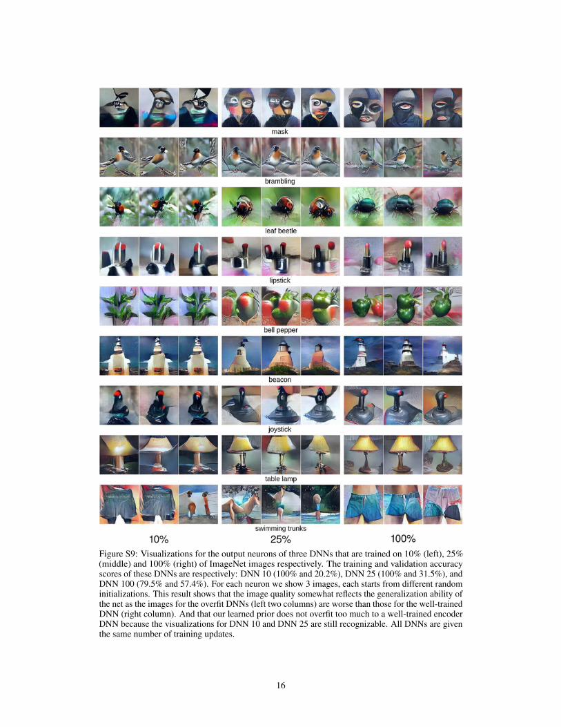
Figure S9: Visualizations for the output neurons of three DNNs that are trained on 10% (left), 25%(middle) and 100% (right) of ImageNet images respectively. The training and validation accuracyscores of these DNNs are respectively: DNN 10 (100% and 20.2%), DNN 25 (100% and 31.5%), andDNN 100 (79.5% and 57.4%). For each neuron we show 3 images, each starts from different randominitializations. This result shows that the image quality somewhat reflects the generalization ability ofthe net as the images for the overfit DNNs (left two columns) are worse than those for the well-trainedDNN (right column). And that our learned prior does not overfit too much to a well-trained encoderDNN because the visualizations for DNN 10 and DNN 25 are still recognizable. All DNNs are giventhe same number of training updates.

16

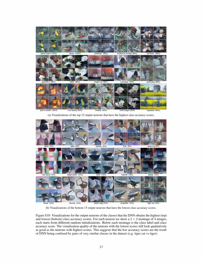
(a) Visualizations of the top 15 output neurons that have the highest class accuracy scores.

(b) Visualizations of the bottom 15 output neurons that have the lowest class accuracy scores.

Figure S10: Visualizations for the output neurons of the classes that the DNN obtains the highest (top)and lowest (bottom) class accuracy scores. For each neuron we show a 2× 2 montage of 4 images,each starts from different random initializations. Below each montage is the class label and classaccuracy score. The visualization quality of the neurons with the lowest scores still look qualitativelyas good as the neurons with highest scores. This suggests that the low accuracy scores are the resultof DNN being confused by pairs of very similar classes in the dataset (e.g. tiger cat vs tiger).

17

Figure S11: Visualizations of optimizing an image that activates two neurons at the same timewith. Top panel: the visualizations of activating single neurons. Bottom panel: the visualizations ofactivating “brambling neuron” and a corresponding neuron shown in the top panel. We found manycombinations that are interesting both artistically and scientifically. In other words, this method canbe a novel way for generating art images for the image generation domain, and also can be used touncover new types of preferred images for a neuron, shedding more light into what it does (here are∼30 images that activate the same “brambling” neuron).

18

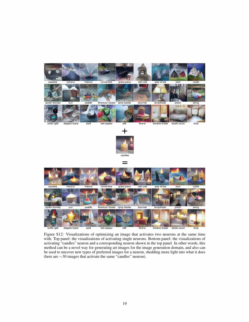
Figure S12: Visualizations of optimizing an image that activates two neurons at the same timewith. Top panel: the visualizations of activating single neurons. Bottom panel: the visualizations ofactivating “candles” neuron and a corresponding neuron shown in the top panel. In other words, thismethod can be a novel way for generating art images for the image generation domain, and also canbe used to uncover new types of preferred images for a neuron, shedding more light into what it does(here are ∼30 images that activate the same “candles” neuron).

19

(a) Prior trained to invert conv3 representations.

(b) Prior trained to invert conv5 representations.

(c) Prior trained to invert fc6 representations.

(d) Prior trained to invert fc7 representations.

Figure S13: Comparison of the results of running our optimization framework with different priors G,each trained to invert from a different layer of an encoder network E. Priors trained to invert featuresfrom fully-connected layers (c, d) of an encoder CaffeNet produces better coherent global structuresthan priors trained to invert from convolutional layers (a, b). These networks are downloaded from[11]. A hypothesis is that each neuron in a lower convolutional layer has a small receptive field sizeon the input image, and only learns to detect low-level features [9, 2]. Thus, optimizing a code at aconvolutional layer results in repeated fragments compared to optimizing at a fully-connected layer,where neurons have learned to care more about global structures [9]. Another orthogonal hypothesisis that the code space at a convolutional layer is much more high-dimensional, making it harder tofind codes that produces realistic-looking images.

20

Figure S14: Visualization of example neuron feature detectors from all eight layers of a CaffeNetDNN [24]. The images reflect the true sizes of the receptive fields at different layers. For eachneuron, we show 4 different visualizations: the top 2 images are from a previous work that harnessesa hand-designed prior called “mean image initialization” [9]; and the bottom 2 images are from ourmethod. This side-by-side comparison shows that both method often agree on the features that aneuron has learned to detect. In overall, our method produces more realistic-looking color and texture.However, the comparison also suggests that our method does not visualize well animal faces (the 3rd& 4th units on layer 6; 1st unit on layer 5; and 6th unit on layer 4). Best viewed electronically, incolor, with zoom.

21

Figure S15: Visualization of example neuron feature detectors from all eight layers of a AlexNetDNN trained to classify 205 categories of places from [32]. The images reflect the true sizes of thereceptive fields at different layers. For each neuron, we show 4 different visualizations. Similarly tothe results from [32], our method also reveals that hidden neurons from layer 3− 5 learn to detectobjects automatically as the result of training the DNN to classify images of scenes. For example, the3rd and 4th unit on layer 5 fires for water towers, and fountains respectively. Interesting, we alsofound that neurons in layer fc6 and fc7 appear to blend different objects together—a similar findingin a different DNN that is trained on ImageNet dataset [9], and also shown in Fig. S14. Best viewedelectronically, in color, with zoom.

22

Figure S16: Visualizations of hidden neurons (one per row) in layer 5 of a DNN trained to classify205 categories of places from [32]. Per row: each of the left 5 images (taken from [32]) highlightsthe region that causes the high neural activation from a real image. This highlighted region is alsogiven a semantic label (shown below each row) by humans from the study in [32]. The right 5 imagesare the visualizations from our method, each produced with a different random initialization. Ourmethod leads to the same conclusions on what a neuron has learned to detect as the method of Zhouet al. [32].

23

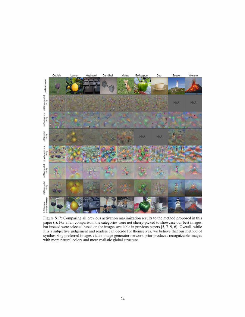
Figure S17: Comparing all previous activation maximization results to the method proposed in thispaper (i). For a fair comparison, the categories were not cherry-picked to showcase our best images,but instead were selected based on the images available in previous papers [5, 7–9, 6]. Overall, whileit is a subjective judgement and readers can decide for themselves, we believe that our method ofsynthesizing preferred images via an image generator network prior produces recognizable imageswith more natural colors and more realistic global structure.

24

Figure S18: For a better and fair evaluation of our method, we show here 120 randomly chosenvisualizations for the output neurons of CaffeNet DNN (the model that we use throughout this paper).

25

(a) Regular ImageNet training images

(b) Cut-up ImageNet training images

(c) Visualizations of neurons that are trained on regular ImageNet images

(d) Visualizations of neurons that are trained on cut-up ImageNet images

Figure S19: Comparison of the visualizations for neurons that are trained on regular ImageNet imagesvs. neurons trained on cut-up images. Our result shows evidence that the learned prior is not sostrong that it always generates beautiful images. Instead, the visualizations seem to reflect closely thefeatures learned by the neurons, here the features of cut-up objects.

26

(a) Regular ImageNet training images

(b) ImageNet training images converted into BRG color space

(c) Visualizations of the neurons that are trained on regular ImageNet images

(d) Visualizations of the neurons that are trained on BRG ImageNet images

Figure S20: Comparison of the visualizations for the neurons that are trained on regular ImageNetimages vs. neurons trained on BRG images. Our result shows evidence that the learned prior is notso strong that it always generates beautiful images. Instead, the visualizations seem to reflect closelythe features learned by the neurons, here the features of images in a completely different color space.

27

(a) Regular ImageNet training images

(b) ImageNet training images that are blurred via Gaussian blur (radius=3)

(c) Visualizations of the neurons that are trained on regular ImageNet images

(d) Visualizations of the neurons that are trained on blurred ImageNet images

Figure S21: Comparison of the visualizations for the neurons that are trained on regular ImageNetimages vs. neurons trained on blurred images. Our result shows evidence that the learned prior is notso strong that it always generates beautiful images. Instead, the visualizations seem to reflect closelythe features learned by the neurons, here the visualizations of the “blurred” neurons often do not havesharp textures, and the fine details are washed out (e.g. “cardoon” neuron). Best viewed with zoom.

28

Figure S22: To test whether our method memorizes the training set images, we retrieved the closestimages from the training set for each of sample synthetic images. Specifically, for each syntheticimage (leftmost column) for an output neuron Y (e.g. lipstick), we find an image among all images ofthe same class Y with the lowest Euclidean distance in pixel space (2nd leftmost), as done in previousworks [22], but also in each of the 8 code spaces of the encoder DNN (layer conv1 to fc8). Thesynthetic images are the result of optimizing the input fc6 code of the DGN prior. While comparingagainst a nearest neighbor among the same class is a much harder test than comparing against anearest neighbor among the entire dataset, we found no evidence that our method memorizes thetraining set images. We believe evaluating similarity in the code spaces of deep representations, whichbetter capture semantic aspects of images, is a more informative approach compared to evaluatingonly in the pixel space.

29