abstract algebra - ::mpbou:: · abstract algebra the word „algebra‟ is derived from the arabic...
TRANSCRIPT
Abstract Algebra
The word „Algebra‟ is derived from the Arabic word „al-jabr‟.
Classically, algebra involves the study of equations and a number of problems
that devoted out of the theory of equations. Then the term modern algebra is
used as a tool to describe the information based on detailed investigations.
Consequently a special branch of algebra namely abstract algebra, a
generalization of modern algebra is introduced in which the algebraic systems
(structures) are defined through axioms.
The present course is divided into three blocks. The first block containing
two units deal with the advanced study of group and ring theory. Then second
block containing two units, introduces the concepts of vector spaces and linearly
independence, basis and dimensions including the theory of linear
transformations in consecutive units 3 and 4. Finally in block III the interesting
properties of a special class of vector spaces called inner product spaces have
been established and it is unit 5.
After the study of this course the students will realize that abstract algebra
allow us to deal with several simple algebraic systems by dealing with one
representative system.

2
In previous classes the students have already studied elementary abstract
algebra in which they have grabbed the elementary knowledge of two algebraic
systems namely groups and rings including their properties. The main aim of
this block is to deal with the further studies of these two systems. Ideally the
goal is to achieve the information regarding groups and rings concerned with
the prescribed course.
Units – 1This unit provides the special case of isomorphism of groups called
automorphism and inner automorphism. Consequently automorphism group is
described. Thereafter we also introduced conjugacy relation, class equation and
counting of the conjugate elements corresponding to the elements of group. In
the end of this unit, we shall discuss that a finite group G has a subgroup of
every prime order dividing the order of group through Cauchy‟s & Sylow‟s
theorems.
Unit – 2This unit presents the study of ring homomorphism and ideal (analogue
of normal subgroup), quotient ring (analogue of quotient group), field of
quotient group of an integral domain and a special class of integral domain
called Euclidean ring. Then we introduced the polynomial rings over rational
field and commutative rings. In the end of the unit, unique factorization domain
has been discussed.
Some self study examples and proof of the theorems are left to the readers to
check their progress.
Block Introduction
3
BLOCK – 1
ABSTRACT ALGEBRA
UNIT – 1 GROUP THEORY
Structure :
1.1Automorphism
1.2Inner Automorphism
1.3Automorphism groups
1.4Conjugacy relation and Centralizer
1.5Normaliser
1.6Counting principle and the class equation of a finite group
1.7 Cauchy’s and Sylow’s Theorems for finite abelian and non abelian groups.
*Points for Discussion/ Clarification
**References
Before describing the main contents of unit, first we shall explain the fundaments concepts of
group theory which are essential to understand the entire unit for convenience. Students may
wish to review this quickly at first and then read the further required part of the prescribed
course.
1.Function : The Notation f : A B to denote a function (or map) from A to B and the value
of f at a is denoted by f(a). The set A is called the domain of f and B is called the codomain
of f.
The set f (A) = {bB| b = f(a),for some aA} is called the range or image of A under f. For
each subset C of B, the set f –1
(C) = { aA: f(a) C} Consisting of the elements of A
mapping into C under f is called the pre image or inverse image of C under f. Let f : AB.
Then
(a) f is injective (or injection or one one) if whenever

4
a1 a2, then f(a1) f(a2)
OR
f (a1) =f (a2), then a1 = a2
(b) f is surjective (or surjection or onto) if for each bB there is some aA such each
that f(a) = b.
(c) f is bijective (or bijection) if f is both injective and surjective
2. Permutation : A permutation on a set A is simply a bijection from A to it self.
3. Binary relation : A binary relation “” on a set A is a subset R of A A and we write
a b if (a, b) R . The relation “” on A is
a) reflexive if a a , for all a A
b) symmictric if a b b a , for all a, b A
c) transitive if a b and b c a c , for all a, b, c A
A relation is an equivalence if it is reflexive, symmetric and transitive.
4.Equivalence Class : If “ ” defines an equivalence relation on A, then equivalence
class of a A is defined to be {x A| x a}. It is denoted by the symbol [a].
i.e. [a] = {x A| x a}. Elements of [a] are said to be equivalent to a.
5.Binary operation or composition : Let G be a non empty set. Then a binary operation
on G is a mapping from G G in to G, defined by
(a, b) ab
i.e. a, b G ab G
Example : Let A = { 1, –1} & B = {1, 2}
Then the multiplication operation „.‟ is a binary operation on A but not B. Since for 2, 2
B 2.2 = 4 B.
6. Group: A non empty set G along with above binary operation is called a group if it
satisfies the following axioms :
G1 For a, b G a b G (Closure axiom)
G2 For a, b, c G (a b) c = a (b c) (associative axiom)
G3 There exists an element e G called an identity element of G such that for all
a G a e = a = e a
G4 For every a G , there exist a–1
G. Such that aa–1
= e = a–1
a .
a–1
is called the inverse of a in G. The axiom G1 is a super flous statement, i.e. It is a binary
composition. G with axiom G1 only is called a groupoid, with G1 andG2 is called semi group
and with G1, G2 and G3 only is called a monoid.

5
7.Commutative or abelian group : A group G is called an abelian or commutative
group if for all a, b G ab = ba
A group G is called finite if it is a finite set , other wise infinite.
8. Order of Group : The number of elements in a group G is called the order of G and
It is denoted by 0(G). The infinite group is said to be of infinite order. The smallest group is
denoted by {c} consisting only the identity element. It is clear that 0 ({e}) = 1.
Example : (i) The set Z (or I) of integers forms an abelian an group w.r.t usual addition of
integers but Z does not form a group w.r.t. multiplication since multiplicative inverse of
every element of Z does not belong to Z.
For example 2 Z but
2–1
= ½ Z /
(ii) The set Q of rationals , R the set of reals are abelian groups w.r.t addition.
(iii) Set of all 2 2 matrices over integers under matrix addition forms an abelian
group.
9. Properties of group : In a group G :
(i) The identity element is unique.
(ii) The inverse of each a G is unique.
(iii)(a–1
)–1
= a , for all a G
(iv) (ab)–1
= b–1
a–1
for all a, b G (Reversal law)
(v) Left cancellation law ab = ac b = c
(vi) Right cancellation law ba = ca b = c for all a, b, c G
10. Complex of a group : Every nonempty subset of a group G is called a Complex of G.
11. Sub Group : A non empty sub set H of a group G is a sub group of G if H is
closedunder products and inverses .
i.e. a, b H ab H and a–1
H
The sub groups H = G and {e} are called trivial or improper sub groups of G and the sub
groups H G and {e} are called nontrivial or proper sub groups of G. It can be easily seen
that the identity of a sub group H is the same as the identity of group and the inverse of a in
H is the same as the inverse of a in G.
Example : The set {1, –1} is a sub group of the multiplicative group {1, –1, i, –i}
(ii) The set of even integers {0, 2, 4, …} is a subgroup of the set of additive
group Z = { 0, 1, 2, ….} of integers.
Criterian for a sub group : A sub set H of a group G is a sub group if and only if (i) H
and (ii) For all a, b H a.b H and for all a H a–1
H

6
OR
For all a, b H ab–1
H
It can also be check that the intersection of two subgroups is a subgroup but
union of two subgroups is not necessarily a subgroup.
12 Order of an Element : The order of an element a G is the least positive integers n
such that
an = e , where e is the identity of G.
Example : Let G = {1, –1. i, –i}. Then G is a multiplicative group.
Now 11
= 1 0(1) = 1
(–1)1 = 1 , (–1)
2 = 1 0 (–1) = 2, i
1 = I, i
2 = –1, i
3 = –i, i
4 = 1 o(i) = 4
(–i)1 = –i, (–i)
2 = –1, (–i)
3 = i, (–i)
4 = 1 0(–i) = 4
13 Cyclic group : If in a group G there exist an element a G such that every element x
G is of the form am, where m is some integer. Then G is a cyclic group and a is called the
generator of G.
Example G = {1, –1, i, –i}
= {i4, i
2, i, i
3}= {i, i
2, i
3, i
4 }
Then G is a cyclic group generated by i.
Note : There may be more than one generators of any cyclic group.
Some useful result of cyclic group:
(i) Every cyclic group is abelian.
(ii) Every subgroup of a cyclic group is cyclic.
(iii) If a is a generator of a cyclic group G. Then 0(G) = 0(a)
(iv) Every group of prime order is cyclic.
14 Cosets: Let H be any sub group of a group G and a G. Then the set
Ha = {ha | h H } is called a right coset of H is G generated by a and
aH = {ah | h H} is called a left coset of H in G generated by a.
Prime No. : An integer p > 1 whose only divisors
are 1 and p other numbers are called composite
numbers. The first prime number is 2. Where 2 is the
only even prime All other prime are odd.
Composite No. : A number is said to be
composite if = r, while |B| > 1, |r| >1

7
Remark: (i) e G He = { he | h H}
= { h | h H}= H
Similarly, eH = H i.e. He = H = eh, means H it self is a right as well as left coset of H in
G.
15 Properties of cosets:
If H is a subgroup of G and
(a) h H , then Hh = H = hH
(b) If a, b are two distinct elements of G, Then
(i) Ha = Hb ab–1 H and aH = bH b
–1 a
H
(ii) a Hb Ha = Hb & a bH aH = bH
(c) Two right (or left) cosets are either disjoint or identical.
(d) If H is a subgroup of G. Then G is equal to the union of all right cosets (or left
cosets) of H in G. i.e. G = H Ha Hb ……, where a, b, c …… are elements of G.
i.e. cosets partition to G.
16 Lagrange’s theorem: The order of each sub group of a finite group divides the order
of group.
17. Index of Sub group: The number of distinct right (or left) cosets of subgroup H of a
group G is called index of H in G. It is denoted by
IG (H) or [G ; H]
By Lagrange‟s theorem
IG (H) = )H(
)G(
0
0
Corollary (i) If a be any element of a finite group G. Then 0(a) | 0(G).
(ii) If G is finite an a G then a 0(G)
= e
18 Normal Subgroup : A subgroup H of a group G is normal in G if
g G & h H ghg–1
H
If gH g–1
= {ghg–1
| G H} . Then H is normal in G if ghg–1
H
Results on normal subgroups:
(a) A subgroup H of G is normal in G iff g Hg–1
= H, g G
(b) A subroup H of G is normal in g iff each left coset of H in G is a right
coset of H in G.
(c) A subgroup H of G is normal in G iff the product of any two right
cosets of H in G is a right coset of H in G.

8
(d) Every subgroup of an abelian group is normal.
19 Quotient group : Let N be any normal subgroup of G. Then the collection G/N of all
right cosets of N in G forms a group under the product of two right cosets. This group is
called the quotient group or a factor group.
Some results on quotient group :
(a) If G is a finite group and N is a normal sub group of G. Then
0)N(
)G(
N
G
0
0
(b) Every quotient group of an abelian group is abelian
(c) Every quotient group of a cyclic group is cyclic.
20 Homomorphism of Groups : Let (G, *) and (G1, o) be any two groups . then a mapping
f : G G1 is called a homomorphism from G into (onto) G
1 if
(i) if is into (onto) (ii) f (a * b) = f (a) o f (b), a, b G.
When the group operations for G and H are not explicitly mentioned, then the
homomorphism condition becomes simply.
f (ab) = f (a) f (b) , for all a, b G
If homomorphism f is onto i.e. f (G) = G′. Then G′ is called homomorphic image G.
Example : Let R be the group of real numbers under addition and R be the multiplicative
group of non zero real numbers and
f : R R0 defined by f (x) = 2x, x R
Then f is a homomorphism .
(ii) If R be the additive group of real numbers and R+ the multiplicative group of positive real
numbers. Then the map f : R+ R defined by
f(x) = log10x is a homomorphism.
Properties of homomorphism : If f : G G′ be a homomorphism of groups and e, e′ be
respectively the identity of G and G′ then
(v) f (e) = e′ (ii) f (a–1) = [f (a)]
–1 for all a G.
Kermel of Homomorphism :
If f : G G′ be a homomorphism of a group G into G′. Then Kernel of f denoted by
k or kf or Kerf is the set of all those elements of G whose image under f is given by the
identites e1 of G
1.
i.e. k = {x G | f (x) = e1 }
9
21 Isomorphism of groups : Let G and G1 be two groups . Then a mapping f : G G
1 is
said to be an isomorphism from G into (onto) G1 if
(vi) f is into (onto).
(vii) f is one one.
(viii)f is a homomorphism.
i.e. the An isomorphism is a special case of homomorphism when it is also one one. If an
isomorphism is onto then G and G1 are said to be isomorphic groups symbolically it is
denoted by G G′.
Some result on homomorphism and isomorphism
(a) If f : G G′ is a homomorphism from a group G into G′ with Kernel K. They K is a
normal sub group of G.
(b) A homomorphism f of a group G into G′ is an isomorphism iff
ker f = {e}
(c) Fundamental theorem on homomorphism: If f is a homomorphism of a group G onto
G′ with kernel k, then G/k G′
OR
Every homomorphic image of a group G is isomorphic to some quotient group.
1.1Automorphism:
Definition 1.1.1. An Isomorphism from a group G onto itself is called an automorphism of
G. i.e. a mapping f : G G is an automorphism if (i) f is one one (ii) ) f is onto (iii)
f is a homomorphism.
The set of all automorphisms of group G is denoted by Aut (G).
Examples:
Example (1): An identity map I : G G defined by I(x) = x , x G is an
automorphism.
Solution: I is obviously a one one and onto map. Also for all x, y G
x. y G
I (x. y) = x. y
I (x. y) = I(x). I(y)
Example (2): Let f : Z Z, where Z is the group of integers with respect to addition, defined
by f(x) = –x, z Z is an automorphism.
Solution: Let f : Z Z is defined by
f (x) = –x, z Z …….(i)

10
f is one one : Let f(x1) = f (x2) , for x1, x2 Z
– x1 = – x2
x1 = x2
f is onto : For any x Z – x Z
f (– x) = – (–x) = x. Thus f is onto
f is a homomorphism : For Any x1 , x2 Z we have
f (x1 + x2) = – (x1 + x2), for x1 + x2 Z
= – x1 –x2
= (–x1) + (–x2)
= f(x1) + f(x2)
Hence f : Z Z is an automorphism.
Example (3) : For any group G, f : G G is defined by
f(x) = x–1
, x G is an automorphism if and only if G is abelian.
Solution : first assume that G is abelian. Let f (x) = f (y) for any x , y G
x–1
= y–1
1111 yx
x = y thus f is one one
Also
f (xy) = (xy)–1
= y–1
x–1
= f (y) f(x)
= f(x) f(y)
Since f is onto . Hence f is an automorphism.
Conversely assume that f : G G is an automorphism. To prove G is abelian , Let x and y be
any two elements of G, then x, y G
x. y G
f (x y) = (x. y)–1
G
= y–.
.1
x–1
(By reversal Law)
= f(y). f (x)
= f (y. x)
x. y = y. x ( f is 1 – 1)
Example 4 : Let G be a finite abelian group of order n (n = odd > 1). Show that G has a
nontrivial automorphism.
Solution : Step – I : Define f : G G by
f(x) = x–1
, x G and prove f is an automorphism as above
Step – II : To prove that f is a nontrivial automorphism
we shall prove that f I

11
Assume if possible f = I
f(x) = I(x) = x
x–1
= x
xx–1
= xx
e = x2 0 (x) = 2 0(x)|2, x G
0(x)= 1 or 0(x) = 2
If 0(x) = 1 , then x = e , which is not true and if 0(x) = 2
0(x) 0(G)
2|0(G)
0(G) is even
Which is again a contradiction, Hence our assumption that f = I is wrong.
f I
CHECK YOUR PROGRESS:
(i) If G is non abelian group then the mapping f : G G defined by
f(x) = x–1
is not an automorphism.
(ii) Let G be the multiplicative group of all positive real numbers. Then a mapping f :
G G defined by f(x) = x2 is an automorphism.
(iii) Let C be the multiplicative group of all non zero complex numbers. Then the
mapping f : C C defined by f(x+iy) = (x–iy) is an automorphism.
Theorem 1.1.2 : Let G be a group and an automorphism of G. If a G is of order o(a) >
0, then 0( (a)) = o(a).
Proof : Suppose that is an automorphism of a group G, and suppose that a G be such
that o(a) = n (i.e. an = e But no lower positive power) . Then
(a)n = (a) (a) (a)……..n times)
= (a, a …..n times)
= (an)
= (e)
= e
Suppose, if possible, (a)m = e for some 0 < m0 < n, then
(a m
) = (a, a …..m times
= (a) (a) (a)……..m times)
= (a) m
= (e)
= (e) ( is homomorphism)
am
= e ( is 1- 1)
This is a contradiction. Thus we conclude that o( (a)) = n.
Hence o( (a)) = o (a)
12
1.2Inner automorphism :
Definition 1.2.1. Let G be a group then for a fixed element g G,
the mapping
Tg : G G defined by
Tg(x) = gxg–1
, x G ………… (i)
is an automorphism of G and is called an inner automorphism of G.
Proof : Tg is one one : For x1 and x2 be any two elements of G such that
Tg (x1) = Tg (x2)
gx1g–1
= gx2g–1
, x G (by (i))
g–1
(gx1g–1
)g = g–1
(gx2g–1
)g
(g–1
g) x1 (g–1
g) = (g–1
g) x2 (g–1
g)
x1 = x2
Tg is one one
Tg is onto : For any y G, an element g–1
y G such that
Tg (g–1
yg) = g (g–1
yg) g–1
= (gg–1
) y (gg–1
)
= eye
= y
Thus Tg is a mapping of G onto G itself.
Tg is a homomorphism : Let x, y G . Then
Tg (xy) = g (xy)g–1
= g(xg–1
gy) g–1
= (g xg–1
) (gyg–1
)
= Tg (x) Tg(y)
Thus Tg is a homomorphism. But Tg is also one one and onto. Hence Tg is an automorphism
of G.
The set of all inner automorphisms of G is denoted by I (G) i.e.
I(G) = { Tg Aut (G) | g G }
= { g xg–1
/ x G}
Remark (i)Since Tg is an automorphism of G defined for a particular element of G.
Therefore Tg is a special kind of an automorphism called an inner automorphism.
Definition 1.2.2 : Self Conjugate element : Let G be a group. An element a G is said
to be self conjugate iff a = x–1
ax, x G
i.e. iff x a = ax, x G
Thus an element a of a group G is self conjugate iff a commutes with every element of G.

13
Definition 1.2.3 : Centre of a group : The set of all self conjugate elements of a group G is
called the centre of G and is denoted by Z (G) or simply by z. i.e.
Z = { z G | zx = xz, x G}
Lemma 1.2.4 The Centre of a group Z is a normal sub group of G.
Proof: We have centre of G i.e. z is given by
Z = { z G | zx = xz x G}
First we shall prove that Z is a sub group of G. Let z1, z2 G . They
z1x = xz1 & z2 x = x z2 x G ………. (i)
Now z2 x = x z2, x G
1
22
1
2
z)xz(z = 1
22
1
2
z)xz(z , x G
x xzz 1
2
1
2
, x G ……(ii)
1
2
z Z, z2 Z
To prove Z is a sub group we shall prove that z1 Zz 1
2 , z1, z2 Z
We have
)xz(zx)zz( 1
21
1
21
= )xz(z 1
21
….(by ii)
= 1
21
z)xz(
= 1
21 z)xz( (by i)
= x )zz( 1
21
, x Z
z1 1
1z Z, z1, z2 Z
Hence Z is a sub group of G.
To prove Z is a normal sub group. Let x be any element of G and z Z . Then
zx = xz x G.
Now
xzx–1
= (xz)x–1
= (zx)x–1
( z x = xz)
= z (xx–1
) = z
But z Z
x z x–1 Z , x G, z Z
Hence Z is a normal sub group of G.
1.3. Automorphism group:
Theorem 1.3.1 : The set of all automorphism of G i.e. Aut(G) forms a group under the usual
composition of mappings.

14
Proof : Let Aut (G) be the set of all automorphisms of G. Since I is a trivial automorphism
of G. therefore I Aut (G). Thus Aut(G) is a nonempty set.
Now we shall prove that Aut(G) forms a group under the composition of mapping first of all
note that Aut(G) is closed under the composition. Let T1, T2 Aut(G) we shall show that T1
T2 Aut(G). Since T1 & T2 are bijective only. Therefore
T1 T2 is also a bijective map.
Also for any x, y G , we have
(T1 T2) (xy) = T1 (T2 (xy))
= T1 (T2 (x) T2 (y))
= T1 (T2 (x)) T1 (T2 (y)
= (T1 T2) (x) (T1 T2) (y)
Thus T1T2 is an automorphism of G.
T1 T2 Aut (G) , for all T1, T2 Aut (G)
Since the composition of mapping is associative, therefore Aut(G) also holds associativity .
Again I, the identities mapping is an automorphism of G.
Therefore I Aut(G) is an identity of Aut(G).
We have only to show that if TAut (G) then T–1
Aut (G),
Now T(T–1
(x)T–1
(y) = (T(T–1
(x) (T (T–1
)(y))
= ((TT–1
)(x) (TT–1
)(y)
= I (x) . I (y)
= xy
This means that
T–1
(xy) = T–1
(x). T–1
(y)
Hence Aut(G) is a group w.r.t. the composition of mappings as composition.
Discussion :We have just established that Aut(G) , the set of all automorphisms of group G
forms a group. It is now a pertinent question whether Aut(G) is a nontrivial group or whether
it consists of trivial automorphism I only. In other words we want to confirm that do there
exist nontrivial automorphisms.
The confirmation is left to the student in the following exercise.
CHECK YOUR PROGRESS:
(I) If G is a group having only two elements, then Aut(G) consists only of I(trivial -
automorphism).
(II) If G has more than two elements than Aut(G) always has more than one elements i.e G
has a non trivial automorphism.
(Hint: See the self study example 2)

15
Definition 1.3.2Permutation: Let G be a finite group of order n. Then a one one mapping
of G onto itself is called a permutation of degree „n‟.
Theorem 1.3.3: Let G be a group . Let A(G) be the group of all permutations on G. Then
Aut(G) , the set of all automorphisms of G is a sub group of A(G).
Proof : Since every member of Aut(G) is a one one homomorphism mapping of a group G
auto G itself i.e. every number of Aut(G) is a permutation on G. Therefore
T Aut (G) T A (G) Aut(G) A(G)
The remaining proof is left to the students.
Hints :
Step (1) Take T1 T2 Aut (G) show that T1 T2 Aut (G) by proving T1T2 is also one
one, onto & homomorphism.
Step (2) Take T Aut (G) & show that T–1
Aut (G) . Hence Aut(G) is a sub group of
A(G).
1.4 Conjugacy relation and Centralizer :
Definitation 1.4.1 : Conjugate element : Let G be a group. An element a G is
called conjugate to an element bG if there exists an element xG such that
a = x–1
bx, for some xG
If a = x–1
bx, then some times we also say that a is transform of b by x.
Remark : Here the element x is not unique .
Definition 1.4.2 Conjugacy Relation: If a is conjugate to b then we write a b and this
relation is known as relation of conjugacy.
Lemma 1.4.3 : Conjugacy is an equivalence relation on G.
Proof To prove that the relation of conjugacy is an equivalence relation on G. We
shall prove that this relation is reflexive, symmetric and transitive.
(i) Reflexivity : Since a = e–1
ae, for each aG . Where e is the identity of G.
a a, for each a G
Thus the relation is reflexive.
(ii) Symmetry : Let a, ,bG be such that

16
a b a = x–1
b x, for some x G
x–1
G such that
xax–1
= x (x–1
bx) x–1
xax–1
= (xx–1
)bxx–1
xax
–1 =b
(x–1)
–1 ax
–1 = b
y–1
ay = b, for y = x–1 G
b a.
Thus the relation is symmetric.
(iii) Transitivity : Let a, b, c G be such that
a b and b c
x, y G such that
a = x–1
bx and b = y–1
cy
a = x–1
(y–1
cy)x
a = (x–1
y–1
) c (yx)
a = (yx)–1
c (yx) (by reversal law)
a = z–1
cz, for z = yx G
a c.
Thus the relation is transitive. Hence the relation is an equivalence relation on G.
Examples 1 Let S3 be a symmetric group on three symbols 1, 2, 3, then
(i) (1, 2, 3) is conjugate of (1, 3, 2)
(ii) (1, 3) is conjugate of (2, 3)
Solution : (2 3)–1
(1 32) (2 3) =
=
1
2
3
3
2
1
1
1
1
2
2
3
3
1
2
3
3
2
1
1
=
3
2
2
3
1
1
1
2
2
3
3
1
2
3
3
2
1
1
=
3
2
2
3
1
1
2
3
1
2
3
1
3
2
1
1
2
3
=
3
2
1
3
2
1=
1
3
3
2
2
1= (1 2 3)
Hence (1 2 3) = ( 2 3)–1
(1 3 2) (2 3)
17
(2) Solution is Left to the students .
Theorem 1.4.5 : Any two elements of an abelian group G are conjugate if and only if they
are equal.
Proof : Let G be an abelian group. First assume that a, b G are conjugate
i.e. a b
a = x–1
bx, for some x G
a = (x–1
b) x
a = (bx–1
)x ( G is abelian)
a = b (x–1
x ) = bc
a = b
Conversely assume that a = b , where a, b G
a = be a = b (x–1
x) a = (bx–1
) x a = (x–1
b) x, (G is abelian)
a = x–1
bx
a b
Hence a and b are conjugate.
Definition1.4.6 Conjugate class: Since an equivalence relation defined on a set decomposes
(partition) the set into mutually disjoint equivalence classes. Hence the relation of conjugacy
on a group G partitions G into mutually disjoint equivalence classes known as classes of
conjugate elements. For an element a G, the conjugate class of a is denoted by C(a) defined
as the set of all those elements of G which are conjugate to a. i.e. C(a) = set of all conjugates
of a
= { x–1
ax |x G}
i.e. C(a) consists of the set of all distinct elements of the form x–1
ax as x ranges over
G.
If G is finite , then the number of distinct elements in C(a) will be finite and denoted by ca
i.e. o C(a) = ca
Note : (i) For the identity e of G.
C(e) = {y G | ye }
= { y G | y = x–1
ex, for some x G}
= {x–1
ex | x G}
= {e}
(ii) If G is an abetian group, then
C(a) = { x–1
ax | x G}
= {ax–1
x | x G}
= {a} , a G
Theorem 1.4.7: Let the conjugacy relation “” defined on G, then for a, b G
18
(i) a C(a)
(ii) b C(a) C(a) = C(b)
(iii) Either C(a) C(b) = or C(a) = C(b)
i.e. two conjugate classes are either disjoint or identical.
Proof : (i) Since the conjugacy relation reflexive on G.
a a, for each a G a C(a) , for each a G.
(ii) Let b C(a) b a ……… (i)
Let x C(a) x a ………(ii)
From (i) and (ii) x a and b a
x a and a b ( is symmetric)
x b ( is transitive)
x C(b) , x C(a)
C(a) C(b) …….. (iii)
Now let y C(b)
y b ………. (iv)
From (i) and (iv) , y b and b a
y a ( is transitive)
y C(a) , C(b)
C(b) C(a) ……… (v)
From (iii) and (v)
C(a) = C(b)
Conversely assume that C(a) = C(b) Since every element belongs to its conjugate class,
therefore
b C(b)
b C(a) (since C(a) = C(b))
Proof (iii) Suppose C(a) C(b) = . Then the theorem is proved .
So let C(a) C(b)
an element say x such that
x C(a) C(b)
x C(a) & x C(b)
x a and x b
a x & x b ( is symmetric)
a b ( is transitive)
a C(b)
C(a) = C(b) (by part (ii) )
Definition 1.4.8: Self conjugate element : An element of a group G is called self
conjugate iff a is the only element conjugate to a.
19
i.e. C(a) = {a}
x–1
ax = a , x G
ax = xa , x G
i.e. a is self conjugate iff a commutes with every element of the group.
Definition 1.4.9 Centralizer : For any non empty subset A of a group G, the Centralizer
C(A) of A is defined as
C(A) = { x G | ax = xa,, a A }
Definition 1.4.10 : Centralizer of Sub group : The centralizer C(H) of a sub group H of a
group G is defined as
C(H) = {x G | hx = xh, h H }
Example: Let G = { 1, i, j, k}. Then G defines a group under usual multiplication
together with i2 = j
2 = k
2 = –1
and ij = –ji = k, jk = – kj= i & ki= –ki = j .G is called
quarterion group. If H = { 1, i} then H is a sub group of G and C(H) = { 1, i}
Theorem 1.4.11: C(H) is sub group of G.
Proof: We have C(H) the centralizer of a sub group H is defined as
C(H) = { x G | hx = xh h H }
Since eh = he, h H
e C(H) C(H)
Let x and y be any two elements of C(H) then
x C(H) hx = xh, h H and y C(H) hy = yh, h H …..(i)
First we shall prove that
y–1
C(H), for any y C(H)
hy = yh, h H
y–1
(hy) y–1
= y–1
(yh)y–1
y
–1h = hy
–1 , h H ………..(ii)
y–1 C(H)
Finally we shall prove that
xy–1
C(H) , x, y C(H)
Now for any h H
(xy–1
) h = x (y–1
h)
= x (hy–1
) by (ii)
= ((xh) y–1
)
= (hx) y–1
by (i)
= h (xy–1
)

20
x y–1 C(H) , x, y C(H)
Hence C(H) is a sub group of G.
1.5 Normalizer:
Definition 1.5.1 Normalizer of an element: The normalizer of an element a G is the set
of all those elements of G which commute with a and is denoted by N(a).
i.e. N(a) = {x G | ax = xa}
Note : (1) Since ex = xe , x G
x N(e) , x G
G N(e)
But N(e) G
N(e) = G
(ii) If G is abelian, then
ax = xa, x G G N(a) But N(a) G
N(a) = G
Theorem 1.5.2 : The normalizer N(a) of a G is a sub group of G.
Proof : We have N(a) = {x G | ax = xa}
Let x1, x2 be any two elements of N(a).
Then x1, x2 N(a)
ax1 = x1a ……….. (i)
and ax2 = x2a ………...(ii)
First we shall show that 1
2
x N(a)
We have ax2 = x2a 1
2
x (ax2) 1
2
x = 1
2
x ( ax2 ) 1
2
x
1
2
x a = a 1
2
x ……… (iii)
1
2
x N(a)
Now we shall prove that x1 1
2
x N(a).
We have a (x1 1
2
x ) = (ax1) 1
2
x
= (x1a) 1
2
x (by (i) )
= x1 (a1
2
x )
= x1 (1
2
x a) (by (iii))
= (x1 1
2
x ) a
x1 1
2
x N(a) , x1, x2 N(a)
Hence N(a) is a sub group of G.
Remark : N(a) is not necessarily a normal sub group of G.
21
Definition 1.5.3 Normalizer of a sub group: For any sub group H of a group g, the
normalizer N(H) of H is defined as
N(H) = { x G | xH = Hx }
Theorem 1.5.4 N(H) is a sub group of H.
The proof of this theorem is left to the students.
Theorem 1.5.5 C(H) N(H). But the converse is not true.
Proof : We have for any sub group H of a group G, the centralizer C(H) and the normalizer
N(H) of a sub group H are defined as
C(H) = { x G | hx = xh, h H }
& N(H) = { x H | xH = xh}
For any x C(H) hx = xh, h H
Hx = xH
x N(H)
C(H) N(H)
How ever C(H) need not be equal to N(H). As considered the quarterian group
G = { 1, i, j, k} and H = { 1, i}
Then N(H) = G and C(H) = { 1, i} showing that C(H) N(H)
Theorem 1.5.6: Let a be any element of G. Then two elements x, y G give rise to the same
conjugate to a if and only if they belong to the same right coset of the normalizer of a in G.
Proof : Let x, y G give rise to the same conjugate of a in G, then
x–1
ax = y–1
ay
x(x–1
ax) y–1
= x (y–1
ay) y–1
axy–1
= xy–1
a
xy–1
N(a)
But N(a) is a sub group of G.
xy –1
N(a) N(a) x = N(a) y ( a Hb Ha = Hb)
x N(a) x = N(a) y ( a Ha)
and y N(a) y = N(a) x
x,y N(a)x = N(a)y
Hence x, y belongs to the same right coset of the normalizer of a in G.
Conversely assume that x, y G belongs to the same right cosets of a in G, Let x, y N(a) z,
for some z G
N(a) z = N(a) x = N(a) y
N(a) x = N(a) y
xy–1
N(a) (Ha = Hb ab–1 H)

22
axy–1
= xy–1
a
x–1
(axy–1
)y = x
–1 (xy
–1 a)y
x–1
ax = y–1
ay
Hence x, y G give rise to the same conjugate of a in G.
1.6 Counting Principle and the class equation of group
Theorem 1.6.1 : Let G be a finite group and a G. Let N(a) denotes the normalizer of a
G and C(a), the conjugate class of a G. Then 0(C(a)) = ))a(N(
)G(
0
0 i.e., number of distinct
elements conjugate to a in G is the index of the normalizer of a in G.
Proof. Let G be a finite group and a G.
To show o(C(a)) = ))a(N(
)G(
0
0
By definition, we have N(a)= {x G: ax = xa}and C(a) = { x–1
ax : x G }
Let M be the set of right cosets of N(a) in G. i.e.
M = { N(a)x : x G}
Let us Define a map f : M C(a) such that f [N(a).x]=x–l
ax xG. Obviously, f is well
defined. To show f is one-one and unto.
(i) f is one-one : Consider
f [N(a) x]=f [N(a) y] , x, y G
x–1
ax = y_1
ay
x (x–1
a x)y–1
= x (y–1
ay) y–1
(xx–1
) (axy–1
) = (xy–1
a) (yy–1
)
e(axy–1
) = (xy–1
a)e
axy–1
=xy–1,
a
a(xy–1
) = (xy–1
)a
xy_1 N(a) a(xy
–1) = (xy
–1)a
xy–1 N(a)
N(a)x = N(a)y
f is one-one.
(ii) f is onto :
For given any x–1
axC(a), N(a) xM such that

23
f (N(a)x) = x–1
ax f is onto.
Hence o (C(a)) = o (M)
= number of distinct right cosets of N(a) in G.
= index of N(a) in G.
= ))a(N(
)G(
0
0, (by definition of index.)
Theorem 1.6.2 : If G is a finite group, then o(G)= ))a(N(
)G(
0
0where this sum runs over one
element a in each conjugate class.
Proof. Since, we know that, the relation of conjugacy is an equivalence relation on the set
G. There fore relation partitions the G into disjoint equivalence classes.
Let C(a),C(b), C(c)… etc. respectively denote the conjugate classes of elements a, b, c ……
G. Also let
0(C(a))=ca,O(C(b))=cb, 0(C(c)) = cc.
Then G = C(a)) C(b) C(c)....
o (G) = o(C(a))+o (C(b))+o (C(c))+...
( C(a) , C(b), C(c) are mutually disjoint)
= o(C(a)) where the sum runs over each elements of conjugate class.
But o(C(a)) = ))a(N(
)G(
0
0 [By theorem 1.6.1]
0(G) = ))a(N(
)G(
0
0 ……..(1)
Remark : The above equation (I) is known as class equation of G.
Theorem 1.6.3. Let Z denote the centre of a group G. Then show that a Z iff
N (a) = G. Also show that if G is finite, then a Z iff 0(N(a)) = 0(G)
Proof. Let Z denotes the centre of group G. Let us first suppose a Z. To show N(a) = G.
Since, we know that N(a) is a subgroup of G and
N(a)={x G : a x = xa}
and Z = {x G : z x = x z, xG.}
Let y G and a Z, then
ay = ya (by definition of Z)
y N{a) G N(a)
But N(a) G G = N(a).
Conversely, let G = N(a), where a G.
24
To show that a G.
N(a) = G G N (a)
y G y N(a) ay = ya
ay = ya, yG a Z.
Now, let G is finite.
To show that a Z 0(G) = 0(N(a))
We have, aZ N(a) = G.
Also, G is finite 0(N(a)) = 0(G)
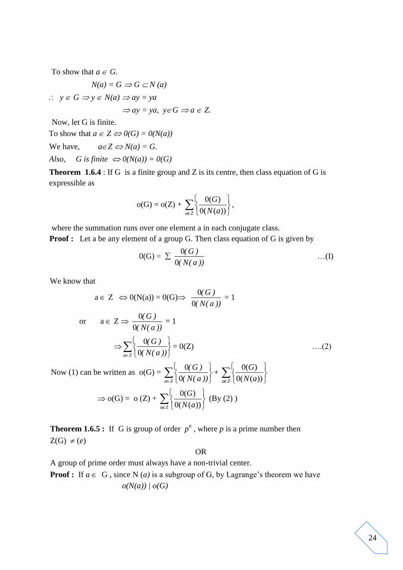
Theorem 1.6.4 : If G is a finite group and Z is its centre, then class equation of G is
expressible as
o(G) = o(Z) +
Za aN
G
))((0
)(0,
where the summation runs over one element a in each conjugate class.
Proof : Let a be any element of a group G. Then class equation of G is given by
0(G) = ))a(N(
)G(
0
0 …(I)
We know that
a Z 0(N(a)) = 0(G) ))a(N(
)G(
0
0 = 1
or a Z ))a(N(
)G(
0
0 = 1
Za ))a(N(
)G(
0
0= 0(Z) ….(2)
Now (1) can be written as o(G) =
Za ))a(N(
)G(
0
0+
Za aN
G
))((0
)(0
o(G) = o (Z) +
Za aN
G
))((0
)(0 (By (2) )
Theorem 1.6.5 : If G is group of order pn , where p is a prime number then
Z(G) (e)
OR
A group of prime order must always have a non-trivial center.
Proof : If a G , since N (a) is a subgroup of G, by Lagrange‟s theorem we have
o(N(a)) | o(G)

25
o (N(a)) | pn, p being prime
o (N(a)) = pn, where na n.
Let Z(G) denote the center of G. Then a Z(G) o(N(a)) = o(G)
pna = p
n
na = n
Let o(Z(G)) = z , writing the class equation of G, we have
pn = o(G) =
nna))a(N(o
)G(o
= nna
))a(N(o
)G(o+ =
nna))a(N(o
)G(o
= )G(Za ))a(N(o
)G(o+
nnn
n
aap
p
= o(Z(G) + nn
n
n
aap
p
= z + nn
n
n
aap
p …..(1)
Since p is a divisor of pn , since na < n for each term in the Σ of the right side, we must have
pan
n
p
p= ann
p
, na < n
p nn
n
n
a
ap
p
Now p | pn and p |
nnn
n
a
ap
p
p | (pn –
nnn
n
a
ap
p)
p | o(Z(G))
Since xe = ex x G e Z (G) and since z 0, it must be a positive integer divisible
by the prime p. But 2 is the least prime number, and so z > 1. This situation demands that
there must be an element, besides e, in Z (G).
Hence Z(G) (e)
Theorem 1.6.6. A group of order p2 is abelian, where p is prime number.

26
Proof. Let G be a group of order p2. Then we have to show that G is abelian. For this, we
shall show that Z = G. (Then G will be abelian, since the centre Z is abelian). Since p is
prime, then Z (e). Therefore, o(Z) > 1. Again since Z is a subgroup of G. Then, by
Lagrange's theorem o (Z) | o(G) i.e., o(Z ) | p2
either o(Z) = p or o(Z) - p2.
If o(Z) = p2
o(Z) = o(G)
Z = G, where Z is abelian
G is also abelian and the result follows.
Now, suppose o(Z). = p, so o(Z) < o(G). Then there must exist an element which is
in G but is not in Z. Let a G and aZ. Since a commutes with itself, a N(a).
Also, N(a) is a subgroup of G. Let xZ so xa = ax
x commutes with a
x N(a).
Thus x Z
x N(a)
Z N(a)
Now a Z a N(a), Z N(a)
o(N(a)) > 0 (Z)
o(N(a)) > p
But o(N(a)) | o(G) = p2 (By Lagrange‟s theorem)
o(N(a)) = p2 (o(N(a))/p
2)
N(a) = G a Z
which is a contradiction. Thus o(Z) = p is not possible
o(Z)=p2. Hence Z = G
G is abelian.
Remark : It can be seen that a group of order 9 is abelian.
For, p = 3 p2 = 3
2 = 9
i.e. o (G) = p2 , where p = 3 is a prime
o (G)=32 = 9 G is abelian. (By above theorem)
1.7 Cauchy’s Theorem and Sylow’s Theorems for finite abelian groups and
Non-Abelian Groups :
Thorem 1.7.1(Cauchy’s Theorem for abelian Groups) : Let G be a finite abelian
group, and let p be a prime. If p |o(G), then there is an element a e G such that ap
= e.

27
Proof. We shall prove this theorem by induction on o(G). In other words, we assume that the
theorem is true for all abelian groups of order less than that of o(G). From this we shall prove
that the result is also true for G. We note that the theorem is obiviously true for group G with
o(G) = 1; i.e., G = {e}.
If G has only improper subgroups; i.e., G has no subgroups H (e), G, then G must be of
prime order since every group of composite order possesses proper subgroups. Now p is a
prime number and p |o(G). So, o(G)= p. Further, we know that every group of prime order
is cyclic. Therefore, each element a e of G will be a generator of G. Hence excluding e, the
remaining p - 1 elements a ( e) of G are such that a0(G)
= e i.e., a p = e.
So suppose that G has proper subgroups N, then N (e), G. Now there arise two possibilities :
either p | o(N) or p o(N).
If p | o(N), by our induction hypothesis, since o(N) < o(G) and N is abelian,
b N, b e such that bp = e. Since b N G, So we have shown that an element b
G, b e"such that
bp = e
Now Let p o(N). Since G is abelian, N is a normal subgroup of G, so G / N is a group.
Moreover,
0 (G/ N) = )N(
)G(
0
0
o(G) = )N(
)G(
0
0 0(N) o(G) = 0 (G/ N) 0(N) (Since N is normal)
Since, p | o(G) and p o(N), it follows from (1) that
P | o(G\N) = )N(
)G(
0
0< 0 (G) [o(N) > 1]
Also, since G is abelian , G/N is abelian. Thus by our induction hypothesis,
an element Nb G/N satisfying (Nb)n
= N, the identity element of
G/N , Nb N; in the quotient group G/N we have o(Nb) = P. We also have
(Nb)p = N, Nb N
NbP =N, Nb N
bp N, b N , b e
Now using Lagrange's theorem, we have
(bp)0(N)
= e
b0(N)p
= e
(b0(N)
)p = e
Let b0{N)
= c. Then certainly cp = e.
28
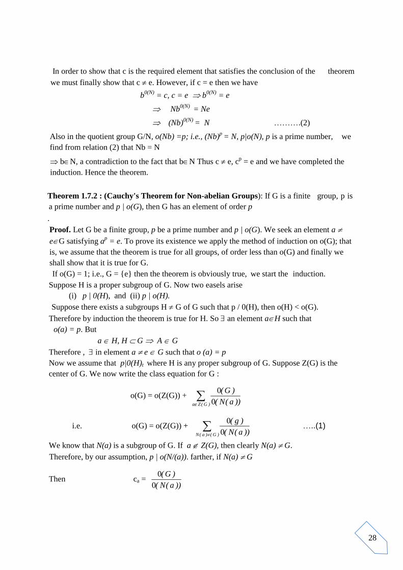
In order to show that c is the required element that satisfies the conclusion of the theorem
we must finally show that c e. However, if c = e then we have
b0(N)
= c, c = e b0(N)
= e
Nb0(N)
= Ne
(Nb)0(N)
= N ……….(2)
Also in the quotient group G/N, o(Nb) =p; i.e., (Nb)p
= N, p|o(N), p is a prime number, we
find from relation (2) that Nb = N
bN, a contradiction to the fact that bN Thus c e, cp = e and we have completed the
induction. Hence the theorem.
Theorem 1.7.2 : (Cauchy's Theorem for Non-abelian Groups): If G is a finite group, p is
a prime number and p | o(G), then G has an element of order p
.
Proof. Let G be a finite group, p be a prime number and p | o(G). We seek an element a
eG satisfying ap = e. To prove its existence we apply the method of induction on o(G); that
is, we assume that the theorem is true for all groups, of order less than o(G) and finally we
shall show that it is true for G.
If o(G) = 1; i.e., G = {e} then the theorem is obviously true, we start the induction.
Suppose H is a proper subgroup of G. Now two easels arise
(i) p | 0(H), and (ii) p | o(H).
Suppose there exists a subgroups H G of G such that p / 0(H), then o(H) < o(G).
Therefore by induction the theorem is true for H. So an element aH such that
o(a) = p. But
a H, H G A G
Therefore , in element a e G such that o (a) = p
Now we assume that p|0(H)t where H is any proper subgroup of G. Suppose Z(G) is the
center of G. We now write the class equation for G :
o(G) = o(Z(G)) + )G(Za ))a(N(
)G(
0
0
i.e. o(G) = o(Z(G)) + )G()a(N ))a(N(
)g(
0
0 …..(1)
We know that N(a) is a subgroup of G. If a Z(G), then clearly N(a) G.
Therefore, by our assumption, p | o(N/(a)). farther, if N(a) G
Then ca = ))a(N(
)G(
0
0

29
o(G) = cao(N(a)) ...(2)
Since p | o(G) and p | o(N(a)), it follows from (2) that
p | ca ; i.e. ))a(N(
)G(p
0
0; if N(a) G and so
G)a(N ))a(N((
)G(p
0
0
P |0(G), and G)a(N ))a(N((
)G(p
0
0
G)a(N ))a(N((
)G()G(p
0
00
p|o(Z(G)) [by(l)]
Thus, Z(G), is a proper subgroup of G such that p | o(Z(G)). But, by our assumption, p is not
a divisor of any proper subgroup of G, and so Z(G) cannot be a proper subgroup of G.
This situation forced us to accept the only possibility left us, namely, that Z(G) = G. But
then G is abelian. We now invoke the Cauchy's theorem for abelian groups which
ensures us. the existence of an element A e G such that ap = e. But p is a prime number
and so o(a) = p. this proves the theorem.
Definition 1.7.3 Sylow’s p-Sub Group :
Definition 1 (p-group) Let p be a fixed prime number. Then a group G is said to be p-group
if every element of G has a order, a power of p.
Definition 2 (p-sub group) Let p be a prime number. Then a subgroup H of a group G is
said to be p-sub group if every element of H is a power of p.
Definition Sylow p-Sub Group: Let G be a group and p be a prime number such that pn
divide order of G and pn+1
does not divide it. Then, a subgroup H of G such that o(H) = pn is
known a Sylow p-sub group of G or p-sylow subgroup of G.

30
Theorem 1.7.4. (Sylow's first Theorem) Let G be a group and p be any prime number and
m be a positive integer such that pm divides o(G). then, there exists a subgroup H of G such
that o(H) = pm.
Proof. We shall prove this theorem by induction. When o(G) = 1, then theorem is obvious.
Further, assume that result is true for all groups with order less than o(G) let pm|0(G). If K is a
subgroup of G such that K G and pm|o(K) , then, by induction H K such that o(H) = p
m.
H K H G.
Therefore, result holds in this case.
Now, assume pm does not divide order of any proper subgroup of G.
Consider class equation of G.
0(G) = 0 [Z(G)] + )G(Za ))a(N(
)G(
0
0
a Z (G) N(a) G
pm
/ o (N(a))
But we have
Pm / o (G) p
m
)a(N
)G(
0
0. 0 (N(a))
p )a(N
)G(
0
0, for all a Z(G) as p
m / o(N(a))
p )G(Za ))a(N(
)G(
0
0
p
)G(Za ))a(N(
)G()G(
0
00 = 0(Z(G))
x Z(G) such that o (x) = p
Let K = { x} Z(G)
K is normal in G
Now 0(G / K ) < 0(G) and pm / o(G) = 0 (G) / K) . 0 (K)
Pm / o(K) and therefore p
m–1 | p
m | o(G | K)
By induction hypothesis there exists a subgroup H / K of G / K such that
O (H / K) pm–1
Therefore o(H) = pm Also , H / K G / K H G. Thus , result is true in this case also
Hence , by mathematical induction theorem is proved.
Remark : If p is prime such that pn | 0(G) and p
n+1 | o(G) , then a p-Sylow subgroup
of G.

31
Theorem 1.7.5 (Sylow’s Second Theorem) : Any two sylow p-subgroup of a finite
group G are conjugate in G.
Proof : Let G be a group and P, Q be Sylow‟s p-sub groups of G such that
O(P) = pn
= o (Q), where pn+1
| O(G)
Let us suppose P and Q are not conjugate in G, i.e. P g Q g–1
for any g G.
It is known that
O (P Q) = )xQxP(o
)Q(o)P(o1
Now, since
P ( x Q x–1
)
O (P (x Q x –1
)) = p m , m n
If m = n, then we have
P (x Q x –1
)) = p
P (x Q x –1
)) P = (x Q x –1
)) [0 (xQx–1
) = 0(Q) = 0(P)]
Which is a contradiction
Therefore, we get m < n and hence 0(P Q) = p2n–m
, m < n , xG which implies
0(P Q) = pn+1
(Pn–m+1
) = multiple of pn+1
Therefore o(G) = x
QPo = multiple of pn+1
pn+1
| RHS pn+1
| o(G)
Which is a contradiction. Hence , P = g Qg–1
, for some g G
Remark : Let P be a Sylow p-subgroup of G. Then the number of Sylow p-subgroup of G
is equal to ))p(N(o
)G(o
Theorem 1.7.6 (Sylow’s third Theorem) : The number of Sylow p-sub groups
of G is of the form 1 + kp where (1+kp) |o(G), k being a non-negative integer.
Proof : Let G be a group and P be a Sylow p-subgroup G. Let o(P) = pn
Now
G = )P(Nx)P(Nxx
PPPPPP
x N(P) P x = xP
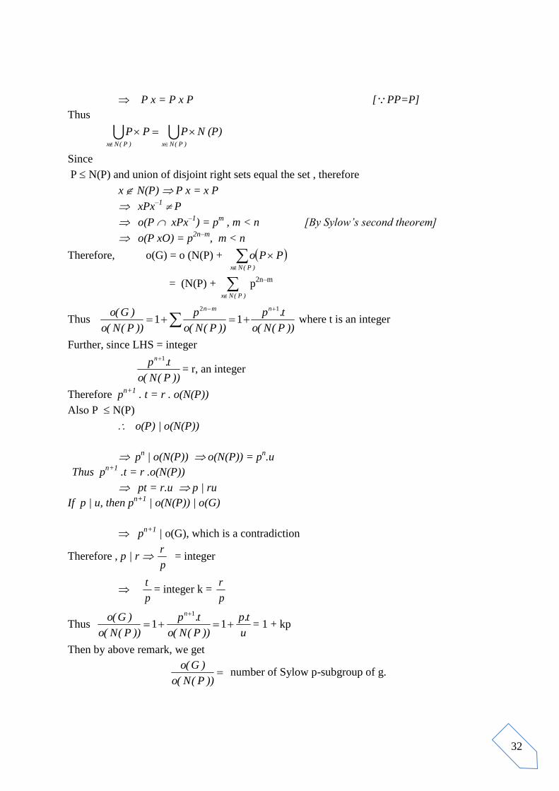
32
P x = P x P [PP=P]
Thus
)P(Nx)P(Nx
PPP
N (P)
Since
P N(P) and union of disjoint right sets equal the set , therefore
x N(P) P x = x P
xPx–1
P
o(P xPx–1
) = pm , m < n [By Sylow’s second theorem]
o(P xO) = p2n–m
, m < n
Therefore, o(G) = o (N(P) +
)P(Nx
PPo
= (N(P) + )P(Nx
p2n–m
Thus ))P(N(o
t.p
))P(N(o
p
))P(N(o
)G(o nmn 12
11
where t is an integer
Further, since LHS = integer
))P(N(o
t.pn 1
= r, an integer
Therefore pn+1
. t = r . o(N(P))
Also P N(P)
o(P) | o(N(P))
pn | o(N(P)) o(N(P)) = p
n.u
Thus pn+1
.t = r .o(N(P))
pt = r.u p | ru
If p | u, then pn+1
| o(N(P)) | o(G)
pn+1
| o(G), which is a contradiction
Therefore , p | r p
r = integer
p
t= integer k =
p
r
Thus u
t.p
))P(N(o
t.p
))P(N(o
)G(o n
111
= 1 + kp
Then by above remark, we get
))P(N(o
)G(o number of Sylow p-subgroup of g.
33
Thus the number of Sylow p-subgroup is of the from 1 + kp = ))P(N(o
)G(o
Hence , ( 1 + kp) | o(G)
Remarks : (i) If o(G) = pn .q. (p q) = 1 then the number of Sylow p-subgroup is 1+kp
where 1+kp | pn q which implies (1+kp|q as (1+kp, p
n) = 1
(ii) Every p-subgroup of a finite group G is contained in some Sylow‟s p- subgroup of G.
(iii)If G is a finite group and P is a p-subgroup of G, then P is Sylow p-subgroup of G if
and only if no p-subgroup of g properly contains P.
POINTS FOR DISCUSSION/ CLARIFICATION:
After going through the block you may like to seek discussion/ clarification on some points.
If so mention these points below:
(I) Points for Discussion:
(II) Points for Clarification:
34
REFERENCES:
1. Topics in Algebra, I.N.Herstien,
2. Algebra (Graduate Texts in Mathematics), Thomas W. Hungerfold, Springer Verlag.
3. Abstract Algebra, David S. Dummit and Richard M. Foote, John Wiley & Sons, Inc..
New York.
4. Basic Algebra Vol. I, N. Jacbson, Hindustan Publishing Corporation, New Delhi
5. A First Course in Algebra, John B. Fraleigh, Narosa Publishing House, New Delhi
BLOCK – 1
ABSTRACT ALGEBRA
UNIT – 2 RING THEORY
Structure :
2.1 Ring Homomorphism
2.2 Ideals and Quotients Rings
2.3 Field of Quotients of an Integral Domain
2.4 Euclidean Rings
2.5 Polynomial Rings
2.6 Polynomials Over the Rational Field
2.7 Polynomial Over the Commutative Rings
2.8 Unique Factorization Domain
Ring Theory:
In general Ring is an algebraic structure with two binary operations namely addition and
multiplication. In fact ring is an abelian group with some extra axioms i.e., it is a generalized
form of a group, therefore many of the concepts and results of group theory can be
generalized to ring. Thus Before describing the main contents of the unit, first we shall
explain the fundamental concepts and elementary results of Ring theory:
1. Ring : An algebraic structure (R, +, ) is said to be ring if (i) (R, +) is an abelian group
(ii) (R, ) is a semi group (iii) Both the distributive laws are satisfied in R.
2. Ring with unity: If there exists multiplicative identity in ring R then it is called ring
with unity.
3. Commutative Ring: R is said to be commutative ring if a b = b a, a, b R.
4. Ring with zero divisors: If there exists a, b R such that a 0, b 0, but ab = 0, then
R is said to be ring with zero divisors and a and b are called zero divisors of R.

35
5. Ring without zero divisors: If there exists a, b R such that ab = 0 either a = 0 or
b = 0, i.e., the product of no two non-zero elements of R is zero, then R is said to be
ring without zero divisors.
6. Elementary properties of ring: For all a, b, c R,
(i) a0 = 0a = 0 (ii) a(-b) = (-a) b = -(ab) (iii) (-a) (-b) = ab (iv) a(b - c) = ab - ac
(v) (b - c) a = ba - ca (vi) For a 0, ab = ac b = c and ba = ca b = c
(Cancellation law).
7. Integral Domain: A commutative ring with unit element and without zero divisors is
called an integral domain.
8. Skew field or division ring: A ring R with unit element is said to be skew field or
division ring if every non-zero element in R has its multiplicative inverse in R.
9. Field: A commutative ring F with unit element is said to be field if every non-zero
element in F has its multiplicative inverse in F.
"A field is necessarily is an Integral domain. However only a finite Integral domain is a
field".
10. Subring: A non-empty subset S of a ring R is called a subring of R if S itself is a ring
under the operations as defined in R.
"The necessary and sufficient conditions for S to be a subring are that (i) a b S,
a, b S and (ii) a b S, a, b S ".
"The intersection of two subrings is a subring. However the union of two subrings is a
subring only when one is contained in the other".
11. Subfield : A non-empty subset K of a field F is called a subfield of F if K itself is a
field under the operations as defined in F.
"The necessary and sufficient conditions for K to be a subfield are that (i) a - b K,
a, b K and (ii) a b-1
K, a, b K ".
2.1. Ring homomorphism.
Definition2.1.1: Homomorphism of Rings. Let R and R` be two rings with two binary
operations additions and multiplication, then a mapping from the ring R into the ring R` is
said to be a homomorphism if
(i) (a + b) = (a) + (b)
(ii) (ab) = (a)(b), for all a, b R.
Remark
Here both rings have same binary operations, in case if R and R” have respectively the
operations + , . and * , o then above conditions (i) and (ii) can be written as
(i) (a + b) = (a)*(b)
(ii) (ab) = (a)o(b)
THINGS TO REMEMBER:
(1) If is surjective, i.e., (R) = R`, then R` is said to be a homomorphism image of R.
(2) If is injective, it is known as isomorphism. If is bijective, then R and R` are
isomorphic and is denoted by the symbol of R R.

36
Definition 2.1.2 Isomorphism of rings:
A homomorphism from a ring R into a ring R is said to be isomorphism if
(i) is one to one
(ii) is onto
i.e, An isomorphism of rings is a special case of homomorphism if it is one-one also
2.1.3 Some useful Results on Homomorphism:
Theorem 1 If is a homomorphism of R into R`, then
(i) (0) = 0`, 0 R, 0` R`, where o and o` are respectively the zero elements of R and R`.
(ii) (-a) = (a), a R.
Proof: (i) Since 0 R and a be any arbitrary element of R, then
a R a + 0 = a
(a + 0) = (a)
(a) + (0) = (a) ( is homomorphism)
Also, 0 + a = a
(0 + a) = (a) (0) + (a) = (a).
(a) + (0) = (a) = (0) + (a), (a) R`.
This show that (0) is the zero element of R`, If 0` is the zero element of R`, then
(0) = 0`.
(ii) Let a be an arbitrary element of R, then –a R therefore,
a + (a) = 0 [a + (-a)] = (0)
(a) + (-a) = (0)
Also, (-a) + a = 0
(-a) + (a) = (0)
Thus (a) + (-a) = (0) = (-a) + (a) (a) R`. Hence (-a) = -(a).
Theorem 2 Every homomorphism image of a commutative ring is a commutative ring.
Proof: Let be a homomorphism from a commutative ring R onto a ring R`, then we shall
have to show that R` is a commutative ring. Let a`, b` be any elements of R`. Since is onto,
then there exists two elements a and b of R such that a` = (a) and b` = (b).
Now, a`b` = (a)(b)
= (ab) ( is homomorphism)
= (ba) ( R is commutative)
= (b)(a) ( is homomorphism)
= b`,a`.
Hence, R` is a commutative ring.
Theorem 3 If is a homomorphism of a ring R into a ring R`, then (R) is a subring of R`.
Proof: Let (a) and (b) be any arbitrary elements of (R) for some a, b R. Since the ring
R is itself a subring so that a – b R and a b R, therefore,
(a) - (b) = (a) + (-b) [ (-b) = -(b)]
= [a + (-b)] (R) ( is homomorphism and a – b R)

37
Now (a)(b) = (ab) (R) ( ab R)
Thus, (a) - (b) (R) and (a) (b) (R).
Hence, (R) is a subring of R`.
Definition 2.1.4 Kernel of a ring homomorphism: Let R and R` be two rings and be a
homomorphism from a ring R into a ring R` then the set of all those elements of R` which are
mapped onto the zero elements of R`, is said to be kernel of and is usually denoted by
ker() or K.
i.e., If 0` is the zero element of R`, then
K= {a R : (a) = 0`}
Since (0) = 0` 0 K
K
2.2 Ideals and Quotient Rings
2.2.1 Ideals
Definition (Left ideal). An additive subgroup S of a ring R is said to be a left ideal of R if
a S, r R r a S .
Definition (Right ideal) . An additive subgroup S of a ring R is said to be a right ideal of R if
a S, r R ar S.
Definition (Ideal). A non empty subset S of a ring R is said to be an ideal of R if it is both
left and right ideal. That is, an additive subgroup S of R is an ideal of R if
a S, r R ra S, ar S.
THINGS TO REMEMBER:
In particular, the subset {0} consisting of 0 alone and the ring R itself are ideals in R. These
two ideals {0} and R are called the improper ideals of R. All other ideals of R are called
proper.
2.2.2 Useful result on Ideals
Theorem 1 If S is an ideal of a ring R, then S is a subring of R
Proof: Since S is an ideal of a ring R, therefore S is an additive subgroup of R and hence
a S, b S a – b S
And
a S, r R ra S and ar S
Also,
a S, b S a S, bR [since S R]
ab S, S being ideal of R.
Theorem 2: The intersection of any two ideals of a ring R is again an ideal of R.
Proof: Let S1 and S2 be any two ideals of a ring R, then we have to show that S1 S2 is also
an ideal of R .
38
Since S1 and S2 are ideal of R so that S1 and S2 both are additive subgroups of R. But
intersection of two subgroups is also a subgroup of R . Thus S1 S2 is also an additive
subgroup of R.
Now, a S1 S2 a S1 and a S2
a S1, r R ra S1 and ar S1 ( S1 being an ideal)
and a S2, r R ra S2 and ar S2 ( S2 being an ideal)
Thus, a S1 S2,r R ra S1 S2 and ar S1 S2.
Hence, S1 S2 is an additive subgroup of R and ra S1 S2 and ar S1 S2 for all a
S1 S2 and r R. Hence, S1 S2 is an ideal of R .
Theorem 3: A field has no proper ideals.
Proof: If F be a field, then we shall prove that its only ideals are {0} and F itself
Let S be an ideal of F and if S = {0}, then in this case the theorem is obviously proved.
Therefore, let S {0} and a be an arbitrary non-zero element of S, then
a S a F ( S F)
a-1
F ( F is a field)
Since S is an ideal of F so that
a S, a-1
F aa-1
S 1 S ( aa-1
= 1)
Now, let x be any element of F, then
1 S, x F 1 . x S x S
F S.
But S F because S being an ideal of R. Hence, S = F and hence only ideals of F are {0} and
F itself.
Theorem 4: If R is a commutative ring and a R, then the set Ra = {ra : r R) is an ideal of
R i.e. Ra is the set of all multiple of a by some element of R.
Proof: In order to prove that R a is an ideal of R, we must show that it is an additive
subgroup of R and if u Ra and r R, then ru is also in Ra. (Here we only need to check
that ru Ra because R is commutative i.e., ru = ur).
Now if u, v Ra, then u = r1a and v = r2a, for some r1, r2 R. Thus
u – v = r1a – r2a = (r1- r2)a Ra ( r1 - r2 R)
Hence, Ra is an additive subgroup of R.
Moreover, if r is any arbitrary element of R and u Ra, then
ru = r(r1a) ( u = r1a)
= (rr1)a Ra ( rr1 R)
Hence, Ra is an ideal of R.
Theorem 5: Let R be a commutative ring with unit element whose only ideals are {0} and R
itself. Then R is a field.
Proof: In order to prove that R is a field we must show that every non-zero element of R has
its multiplicative inverse in R.

39
Let a R and a 0 and consider a set Ra = {ra: r R} then Ra is an ideal of R (By
Theorem 4). But R is a commutative ring with unit element having only ideals {0} and R
itself. Therefore, either Ra ={0} or Ra = R. Since 1 R so that 0 a = 1. a Ra, thus
Ra {0} and hence only possibility is that Ra = R. This implies that every element in R is a
multiple of 'a` by some element of R. But 1 R so that it is also a multiple of a. That is, there
exists an element b R such that ba = 1. But R is commutative and every non-zero element
in R has its multiplicative inverse in R. Hence R is a field.
Solved Examples:
Example 1 If S is an ideal of R and 1 S, prove that S = R.
Solution: Since S is an ideal of R so that S R.
Let a be any arbitrary element of R . S being an ideal of R and 1 S, then
1 S, a R a.1 S
a S.
Thus, R S. But S R. Hence, S = R.
Example 2 If S is an ideal of R, let r(S) = {x R: xa = 0, a S}. Prove that r(S) is
an ideal of R.
Solution: Since 0 R such that 0a = 0, it follows that 0 r(S). Thus r(S) is nonempty. Now
if u, v are any elements of r(S), then ua = 0 and va = 0 where a S, then
(u - v)a = ua - va = 0 - 0 , a S
Thus, u v r(S). Hence, r(S) is an additive subgroup of R.
Let r1 be any arbitrary element of R and u r(S), then ua = 0, a S. Since S being an
ideal of R, therefore,
a S, r1 R ar1 S and r1a S
Then, (r1u)a = r1(ua) = r10 = 0
i.e., r1u r(S)
Also (ur1)a = u(r1a) = 0 ( u r(S) and r1a S so u(r1a) = 0)
i.e., ur1 r(S).
Thus, r(S) is an additive subgroup of R and r1u r(S) and ur1a S
Hence, r(S) is an ideal of R .
Theorem 6 If is a homomorphism of a ring R into a ring R` with kernel K, then K is an
ideal of R.
Proof: By the definition of kernel of a homomorphism, we have
K = {a R : (a) = 0`, where 0` is the zero element of '}.
Now we shall show that K is an ideal.
Let x, y be any arbitrary element of K, then x, y R and (x) = 0`, (y) = 0`.
Now (x - y) = [x + (-y)]
= (x) + (-y) ( is homomorphism)
= 0` - 0` = 0`.
Thus, x – y K, therefore, K is an additive subgroup of R. Moreover, if r be any arbitrary
element of R and a K, then
(ra) = (r) (a) ( a is homomorphism)

40
= (r).0` ( (a) = 0`)
= 0`.
Thus, ra K. Similarly ar K. Hence, K is an additive subgroup of R and ra K and ar
K for all r R, a K. Consequently, K is an ideal of R.
2.2.3 Quotient Ring:
Definition: Let R be ring and S be ideal of R, then the algebraic structure
[R/S,‟+”.‟} where, R/S = {a + S : a R} and the operations „+‟ and „,‟, on R/S defined by
(a + S) + (b + S) = (a + b) + S
and (a + S) . (b + S) = a. b + S , a, b R
forms a ring. This ring is called the quotient ring of R with respect to the ideal S. the quotient
ring is also known as residue class ring or factor ring.
Remarks:
(1) Zero element of R/S is S.
(2) unit element of R/S is S + 1
(3) S + a = S + b a b S.
Theorem 1 Let R be a ring and S an ideal of R. Then the set of cosets of S in R
R/S = {S + a ; a R}
is a ring under the operations “+” and “,” which are defined as follow : for all
S + a, S + b R/S
(S + a) + (S + b) = S + (a + b) ……(1)
(S+ a) . (S + b) = S+ a. b. ……(2)
Proof: First we shall show that the operations of addition and multiplication in R/S
are well defined.
Addition is well defined. If S +a = S + a` and S + b = S + b`, then we shall prove
that
(S + a) + (S + b) = (S + a`) + (S + b‟)
Now S + a = S + a` a` S + a ( H + a = H + b a H = b)
s S such that a` = s + a
and S + b = S + b` b` S + b
t S such that b` = t + b.
a` + b` = (s + a) + (t + b) = (s + t) + (a + b)
(a + b`) (a + b) = s + t S
S + (a` + b`) = S + (a + b)
(S + a`) + (S + b`) = (S + a) (S + b).
Thus the addition in R/S is well defined.
Multiplication is well defined. With above notation, we shall prove that
(S + a) (S + b) = (S + a`) (S + b`).
We have a‟b‟ = (s + a) + (t + b)= st + sb + at+ ab
a` b` ab = st + sb + at. ……(1)
Since S is an ideal we have
41
a, b R and s, t S st S, sb S, at S
st + sb + at S
a`b` ab S [by 1]
s + a`b` = S + ab
(S + a`) (S + b`) = (S + a) (S + b)
Thus the multiplication in R/S is well defined.
(R1), (R/S,t) is an Abelian group :
R11. Closure property. Let S + a, S + b R/S. Then
S + a, S + b + R/S a, b R
a + b R
S + (a + b) R/S
(S + a) + (S + b) R/S.
R12. Addition is associative. Let S + a, S + b, S + c R/S. then
(S + a) + [(S + b) + (S + c)] = (S + a) + [S + (b + c)]
= S + [a + (b + c)] = S + [(a + b) + c]
= [S + (a + b)] + (S + c)
= [(S + a) + (S + b) + (S + c)].
R13. Addition is commutative. Let S + a, S + b R/S. Then
(S + a) + (S + b) = S + (a + b) = S + (b + a) = (S + b) + (S + a).
R14. Existence of additive identity. For each S + a R/S, S = S + 0 R/S such that
(S + a) + (S + 0) = S + (a + 0) = S + a = S + (0 + a)
= (S + 0) + (S + a).
S is the additive identity of R/S.
R15. Existence of additive inverse.. Let S + a R/S.
Then a R a R. Therefore, S + ( a) R/S.
Also, (S + a) + [S + ( a)] = S + (a + ( a)] = S + 0 = S.
S + ( a) is the additive inverse of S + a.
(R2). (R, ) is a semi-group :
R21. Closure property. Let S + a, S + b R/S. Then
S + a, S + b R/S a, b R
ab R
S + ab R/S
(S + a) (S + b) R/S.
R22. Multiplication is associative. Let S + a. S + b, S + c R/S. Then
(S + a) [(S + b) (S + c)] = (S + a) (S + bc)
= S + [a (bc)] = S + [(ab) c]
= (S + ab) (S + c)
= [(S + a) (S + b)] (S + c).
R3. Distributive laws :
R31. Left distributive law. We have
(S + a) [S + b) +(S + c)] = (S + a) [S + (b + c]
= S + [a (b + c)] = S + (ab + ac)
= (S + ab) + (S + ac)

42
= (S + a) (S + b) + (S + a) (S + c).
R32. Right distributive law. We have
[(S + a) + (S + b)] (S + c) = [S + (a + b)] (S + c)
= S + [(a + b) c] = S + [ac + bc]
= (S + ac) + (S + bc)
= (S + a) (S + c)+ (S + b) (S + c).
Therefore, R/S forms a ring under the two compositions “+” and “.” as defined in (1) and (2).
The ring R/S is called the quotient ring (or factor ring) of R with respect (relative) to S.
Theorem 2: Fundamental theorem on homomorphism of rings:
Every homomorphic image of a ring isomorphic to some residue class ring (quotient ring).
Or
If f is a homomorphism from a ring (R, +, .) onto a ring (R`, + „, .‟), then
(R/K, +, .) (R` , +‟, . „).
Proof: Let R` be a homomorphic image of ring R and f : R R‟ be the homomorphism of R
onto R‟ with kernel K. Then K is and ideal of R. Therefore, R/K is the ring of residue classes
of R with respect to K.
We now prove that
R/K R`.
If a R, then K + a R /K and f(a) R` . Now consider a mapping
: R/K R` such that
(K + a) = f(a) a R.
is well defined: If a, b R and K + a = K + b, then we shall prove
(K + a) = (K + b).
Now, K + a = K + b
a – b K
f(a – b) = 0` [zero element of R`]
f[a + (-b) = 0`
f(a) +‟ f(-b) = 0`
f(a) – f(b) = 0`
f(a) = f(b)
(K+ a) = (K + b).
is well defined.
is one-one: Here
(K + a) = (K + b)
f(a) = f(b)
f(a) – f(b) = 0`
a – b K
K + a = K + b.
is one-one
is onto: Ler y R` be arbitrary. Then y = f(a) for some a R because f is onto on R`.
Now K + a R/K and (K + a) = f(a) = y.
Hence is onto on R`

43
Finally, [(K + a) + (K + b)] = [K + (a + b)]
= f(a + b)
= f(a) + f(b)
= (K + a) +‟ (K + b).
Also [(K + a) .(K + b)] = (K + a .b)
= f(a . b)
= f(a) .‟ f(b)
= [(K + a)].‟ [(K + b)]
is an isomorphism of R/K onto R`.
Hence, R/K R.
Definition 2.2.4 Principal Ideal:
An ideal S of a ring R is said to be principal ideal if it is generated by element of S
i.e., if a S is such that every element of S is a multiple of a, then S = {a} is a principal ideal
generated by a .
If R is a ring with unity, then the ideal generated by 1 i.e., {1} is the ring R itself, because r .
1 = r, r R. Therefore, the ring R itself is called the unit ideal.
Also, the ideal generated by the zero element of R i.e., {0} is called null ideal, because {0}
consists of the zero element alone.
Remarks
(1) Every ring R has at least one principal ideal, namely (0).
(2) Every ring with unit element has at least two principal ideals, namely (0) and (1).
Theorem 3 If R commutative ring with unity aR, then the set S = {ra : r R} is a principal
ideal of R generated by the element a i.e., S = {a}.
Proof. Since a R and 1 R, then by definition of S, 1 . a = a S.
Now we shall prove that S is an additive subgroup of R.
Let u and v be any two element of S, then
u = r1a and v = r2a for some r1, r2 R
Consider u – v = r1a – r2a
= (r1 – r2)a (By right distribution law)
u – v S as = r1 – r2 R.
Thus S is an additive subgroup of R.
Now we shall show that for r R, u S ru S and ur S.
But R is a commutative ring so it is sufficient to prove that ru S.
Consider, ru = r(r1a) ( u = r1a)
= (rr1)a
ru S as rr1 R.
Hence, S is an ideal of R.
Now we shall prove that S = (a).
Let ra S and let T be an ideal of R containing a, then.
a T, r R ra T

44
S T.
Hence, S is a principal ideal of R generated by the element a.
Definition 2.2.5 Principal Ideal Ring:
A commutative ring R with unity having no zero divisor is called a principal ideal ring if
every ideal of R is a principal ideal. i.e., every element of R is generated by some element of
itself.
Remark:
An ideal generated by a single element is called principal ideal and the ring whose every ideal
is a principal ideal is called principal ideal ring.
Theorem 4 The ring of integers is a principal ideal ring.
Proof: Let {Z, +,.} be a ring of integers. Obviously Z is a commutative ring with unit
element having no zero divisors. We have to prove that Z is a principal ideal.
Let S be any ideal of Z and if S = {0} then obviously S is a principal ideal as it is
generated by single element 0. So assume that S {0},therefore, S contains at least one non-
zero integer, let it be „a`. Since S is an additive subgroup of z so a S - a S. This
implies that S contains at least on position integer as one of a and –a is positive.
Let S+ denote the set of all positive integers of S, obviously S+ , therefore, by well
ordering principal (Zorn‟s lemma), S+ must possess a lest positive integer.
Let n be any integer in S, then by division algorithm, there exist integers q and r such
that
n = mq + r, where 0 ≤ r< m.
Now m S, q Z mq S [ S is an ideal]
and n S, mq S n – mq S [ S is an additive subgroup of Z]
r S.
But 0 ≤ r < m and m is assumed to be least positive integers of S. Therefore, r = 0 so that
n = mq.
Thus, n S n = mq for some q Z.
Hence, S is a principal ideal of Z generated by the element m. Since S is an arbitrary ideal of
Z therefore, every ideal of Z is a principal ideal. Hence, Z is a principal ideal ring.
Theorem 5 Every field is a principal ideal ring.
Proof: Since a field has no proper ideals, therefore its only ideals are {0} and the field itself.
The ideal {0} is a principal ideal and the field itself is also principal ideal as it is generated by
1. Hence, both these ideals of field are principal. Therefore, every field is a principal ideal
ring.
Divisibility in an Integral Domain
Definition 2.2.6: Let a be a non-zero element of a commutative ring R. Then a divides b R,
if there exists an element c R such that b = ca.
We shall use the symbol a | b to represents the fact that “a divides b”.

45
In particular, if a 0 and a = a . 0, then a | 0 this implies that every non-zero element of R is
a divisor of its zero element.
Theorem 6 If R is a commutative ring, then
(i) a | b and b | c a | c i.e., relation of divisibility in R is transitive relation.
(ii) a| b and a | c a | (b + c)
(iii) a | b a | bx, x R.
Proof.: (i) a | b b = am, for some m R and b | c c = bn, for some n R
c = bm = (am)n = a(mn)
a | c as mn R
(ii) a | b b = am for some m R and a | c c = an for some n R
b + c = am + an = a(m + n)
a | (b + c) as m + n R.
(iii) a | b b = an, for some n R
bx = anx, for all n R a | bx, for all nx R.
Definition 2.2.7 Units:
Let R be a commutative ring with unity i.e., 1 R. Then an element a of R is said to be unit
in R if there exists an element b R such that ab = 1.
Maximal Ideals:
Definition 2.2.8 A proper ideal S of a ring R is said to be maximal ideal of R if it is not
strictly contained in any other proper ideal of R i.e. .A proper ideal S of a ring R is said to be
maximal ideal of R if T is any other proper ideal of R such that either S = T or T = R. i.e. A
proper ideal S of a ring R is said to be maximal ideal of R if there exists no proper ideal
between S and R.
Theorem 7 An ideal S of a commutative ring R with unity is maximal if and only if the
quotient ring R/S is a field.
Proof: Since R is a commutative ring with unity so that R/S is also commutative ring with
unity. In order to show that R/S is a field, we only need to show that every non-zero element
of R/S has its multiplicative inverse in R/S.
Let S be a maximal ideal of R and let S + a be any non-zero element of R/S, i.e.,
S + a a + S.
Let (a) be an ideal of R. Since the sum of two ideals is again an ideal of R so that
S + (a) and (a) + S are again ideals.
Since S is maximal, so that we must have S + (a) = R.
But I R, then for some b S such that b + a = 1 for some R
b = 1 = a
1 - a S ( b S)
S + a = S + 1
(S + ) (S + a) = S + 1
46
Similarly, (S + a)(S + ) = S + 1 ( R/S is
commutative)
Therefore, (S + a)-1
= (S + ) R/S.
Hence, every non-zero element of R/S has its multiplicative inverse and hence R/S is a field.
Conversely, let R/S be a field. Now we shall prove that S is maximal.
Let T be any ideal of R properly containing S and let a be any arbitrary element of R not in S,
then a S S + a S. Thus S + a is a non-zero element of R/S.
Now b be any element of T not in S, then S + b is again a non-zero element of R/S. Since R/S
is a field so that
S + b R/S (S + b)-1
R/S
Now (S + a) R/S, (S + b) R/S (S + a)(S + b)-1
R/S
(S + a)(S + b-1
) R/S
s + ab-1
R/S ab-1
R
Since T is an ideal of R, then b T, ab-1
R ab-1
b T a . 1 T a T.
a R a T.
Thus R T. But T R. Therefore, T = R. Hence, there is no ideal of R between S and R.
Hence S is a maximal ideal of R.
Remark: A ring R is a field if and only if its zero ideal is a maximal ideal, since a field has
no proper ideal.
2.3 Field of quotient of an integral domain:
Definition2.3.1 Quotient in a Field : Let (F, +,) be a field and a, b F. Then the solution
a-1
b or ba-1
of the equation ax = b in F is called quotient in F and is denoted by b
a.
Definition 2.3.2 The Field of Quotient:
Let (D, +, ) be a commutative ring without zero divisors, then we shall show that (D,+,) can
be imbedded into a field (F, +','), i.e., a field (F, +', ')in which contains a subset D'
isomorphic to D. We shall form a field (F, +',') with the elements of D and there will be
subset D' in this field F such that D' is isomorphic to D. This field (F, +',') is called field of
quotient of (D, +,) or quotient field of (D, +,).
Construction of the Quotient Field:
We know very well about the ring of integers (I, +,). By the set of rational number,
We mean the set of quotients of elements of I. Thus Q = : , 0p
p q I and qq
. If we
identify the rational numbers...., 3 2 1 0 1 2 3
, , , , , , ....1 1 1 1 1 1 1
by integers…-3,-2,-1, 0, 1, 2, 3,....,
then I Q. Also (Q, +,) is a field. If a/b and c/d Q, then we define the following :
(i) a c
b d if and only if a . d = b . c.

47
(ii) . .
.
a c a d b c
b d b d
(iii) .
..
a c a c
b d b d
Theorem 8 A commutative ring without zero divisors can be imbedded into a field.
Or
Every integral domain can be imbedded into a field.
Proof: Let (D, +, ) be a commutative ring without zero divisors and D0, be the set of non-
zero elements of D. If S = D × D0, i.e., if S be the set of all ordered pairs (a, b); where a, b
D and b 0. Then the relation ~ defined by (a, b) ~ (c, d) if and only if a . d = b . c
is an equivalence relation in S.
Reflexivity. since D is commutative ring, therefore
a.b = b.a a, b D.
Thus (a, b) ~ (c, d) (a, b) S.
Symmetric. Here, we have
(a, b) ~ (c, d) a . d = b . c
d . a – c . d [commutative law]
c . b = d . a
(c, d) ~ (a, b).
Transitivity. Let (a, b) ~ (c, d) and (c, d) ~ (e, f), then
(a, b) ~ (c, d) and (c, d) ~ (e, f)
a . d = b . c and c . f = d . e
(a . d) . f = (b . c) . f and b . (c .f) = b . (d. e)
(a . d) . f = b . (d . e) [ (b . c). f = b . (e. f)]
a . (d . f) = b.(d . e)
a . (f . d) = b . (e . d) . [commutative law]
(a . f) . d = (b . e) . d
(a. f). d (b . e). d = 0
(a . f b . e). d = 0
a . f b . e = 0 [ d 0 and D is without zero divisors]
a . f = b . e
(a, b) ~ (e, f).
Therefore, the relation ~ is an equivalence relation in S and it will partition S into disjoint
classes. Then
a
b= {(c, d) S : (c, d) ~ (a, b)}.
Obviouslya c
b d if and only if (a, b) ~ (c, d),
i.e., a . d = b . c.
Also .
.
a a x
b b x x D0, since

48
a . (b . x) = b . (a . x) (a, b) ~ (a . x, b . x).
These equivalence classes are our quotients. Let F be the set of all these quotients, i.e.,
: ( , )a
F a b Sb
.
Now we shall define the operations +' and ' in F as:
. . .' .'
. .
a c a d b c a c a cand
b d b d b d b d
.
Since D is without zero divisors, therefore
b 0, d 0 b . d 0.
. . .
. .
a d b c a cand
b d b d
both are the elements of F. The F is closed with respect to +' and .' and
now we shall show that +' and .' both are well defined. For this, if
'
'
a a
b b and
'
'
c c
d d then
' ' ' '' ' .' .'
' ' ' '
a c a c a c a cand
b d b d b d b d .
Thus '
'
a a
b b a .b` - b .a`
and '
'
c c
d d c .d' = d .c'.
Now, we shall show that
' '' '
' '
a c a c
d d b d .
For this we shall show that
. . '. ' '. '
. '. '
a d b c a d b c
b d b d
,
i.e., (a .b + b . c).(b` . d') = (b . d) . (a` . d' + b` . c').
Now (a . d + b . c).(b` . d')
= (a . d) . (b` . d') + (b . c).(b` . d')
= (a . b`) . (d . d') + (b . b`) . (c . d')
= (b . a`) . (d . d') + (b . b`) . (d . c') [ a . b ' = b . a` and c . d' = d . c']
= (b . d) . (a` . d') + (b . d) . (b` . c')
= (b . d) . (a` . d' + b` . c').
Again to show : ' '
.' .'' '
a c a c
b d b d . For this we shall show that
. '. '
. '. '
a c a c
b d b d ,
i.e., (a . c) . (b` . d') = (b . d) . (a` . c').
Therefore (a . c) . (b` . d') = (a . b`) . (c . d')
(b . a`) . (dc')
= (b . d) . (a` . c').

49
Thus +' and ' both are well defined. Now, we shall show that (F, +‟, ‟ ) is a field.
Associativity of addition: Here, we have
. .' ' '
.
a c e a d b c e
b d f b d f
( . . ). ( . ).
( . ).
a d b c f b d e
b d f
( . ). ( . ). ( . ).
( . ).
a d f b c f b d e
b d f
.( . ) ( . . )
.( . )
a d f b c f d e
b d f
. .'
.
a c f d e
b d f
' 'a c e
b d f
.
Commutativity of addition: Here, we have
. . . .
' '. .
a c a d b c a b b c c a
b d b d d b d b
.
Existence of additive identity: Here0
a F where a 0. If
c
dis any element of then
0 0. . 0 . .'
. . .
c d a c a c a c c
a d a d a d a d d
[ (a .c) .d (a .d).c]
0
a s additive identity and
0 0
a b a, b D0.
Also 0d
d a if and only if, c . 0 = d . 0, i.e., c = 0.
Existence of additive inverse: If a
b F, then
a
b
F.
Also, here 2
( ) . .'
a a a b b a
b b b
=2
0 0
b a [ 0 .a = b
2 .0]
a
b
is additive inverse of
a
b.
Associativity of multiplication: Here
..' .' .'
.
a c e a c e
b d f b d f
= ( . ). .( . )
( . ). .( . )
a c e a c e
b d f b d f

50
= .' .'a c e
b d f
.
Commutativity of multiplication: Here
. ..' .'
. .
a c a c c a c a
b d b d d b d b .
Existence of multiplicative identity: Here
a
b F where a 0. Also if
c
d F, then
..'
.
a c a c c
a d a d d [ (a .c, a .d)~ (c . d) because (a . c) .d= (a . d) . c]
a
a is the multiplicative identity
and a b
a b a, b D0.
Existence of multiplicative inverse of non-zero elements of F:
Let a
bbe any non-zero element of F, then a 0.
b
a F.
Also . .
.,. .
a b a b a b a
b a b a a b a = unit element.
b
ais the multiplicative inverse of
a
b.
Distributivity of multiplication over addition: Here
. . ( . . )
.' ' .'. .( . )
a c e a c f d f a c f d e
b d f b d f b d f
= ( . ) .( . )
.( . )
a c f a d e
b d f
= ( .( . ) .( . )).( .( . ))
( .( . )).( .( . ))
a c f a d e b d f
b d f b d f
= ( .( . )) ( .( . )) ( .( . )).( .( . ))
(( . ). ).( ( . ). )
a c f b d f a d e b d f
b d f b d f
= ( . ). ( . ).
'( . ). ( . ).
a c f a d e
b d f b d f
= . .
' .' ' .'. .
a c a e a c a e
b d b f b d b f
Similarly, we can prove other distributive law.
(F, +',') is a field, This field is called the field of quotients of D.

51
Now we shall show that field F contains a subset D' such that D is isomorphic
to D'.
Let D' = : , ( 0)ax
F a x Dx
, then D' F. If x 0, y 0 are the elements of
D, then ax ay
x y since axy xay.
Therefore if x is some fixed non-zero element of D, then we can write
D' = :ax
F a Dx
Now we shall show that the function : D D' defined by the rule
(a) = ax
x a D,
is isomorphic to D onto D'.
is one-one: Here
(a) = (b) ax bx
x x
axx = xbx
ax2 = bx
2
(a - b)x2 = 0
a b = 0 ( x2 0)
a = b.
is one-one.
is onto: D'. If ax
x D', then a D. Also
(a) = ax
x
Also, (a + b) = 2( )a b x
x
= 2 2
2
ax bx
x
= 2
axx xbx
x
= ax bx
x x
= (a) + (b)
and (ab) = 2
2
( ) ( )ab x ab x
x x
= 2
( )( )ax bx
x

52
= ax bx
x x= (a)(b)
D D‟.
If we identify D by D‟, i.e., if , , ,....,ax bx cx
x x x in place of a, b, c,…., in F, then we see that F
contains D. Thus the field F of the quotients of D is a field which contains D.
Theorem 9 If K is any field containing the integral domain D, then K contains a subfield
isomorphic to the quotient field F to D.
Proof: Since D is an integral domain, therefore D is a commutative ring without zero
divisors. Let K by any field containing D. If 0 b D, then
a K, 0 b K ab-1
K.
Consider a subset K‟ of K containing the elements of the type ab-1
where a, b D and b 0.
Hence K‟ = {ab-1
K : a,0 b D}.
We shall prove that K‟ is a subfield of K and K‟ F, where F is the quotient field of D.
Let ab-1
K‟, cd -1
K‟, then 0 b, 0 d D.
Now
ab-1
cd-1
= add-1
b-1
– cbb-1
d-1
= (ad – bc) d-1
b-1
= (ad bc)(bd)-1
K‟ [ ad – bc D and 0
bd D]
Again let 0 cd-1
K’, then c 0 and
(ab-1
) (cd-1
)-1
= ab-1
dc-1
= adb-1
c-1
= ad (cb)-1
K‟ [ ad D and 0 cb
D]
Thus K‟ is a subfield of K.
We now show that F the quotient field of D, is isomorphic to K‟. Here
: ,0a
F a D b Db
.
Now consider a mapping : F K' defined by
a
b
= ab-1
a
b F.
is one-one. Let ,a c
b d F. Then
a
b
= c
d
ab-1
= cd-1
ab-1
bd = cd-1
bd
ad = cb d-1
d
ad = bc
(a, b) ~ (c, d)

53
a c
b d .
is one-one.
is onto K'. If ab-1
K' be any element then an element a
b F such that
a
b
= ab-1
Thus is onto K'.
Also a c
b d
=
ad bc
bd
= (ab + bc)(bd)-1
= (ad + bc) d-1
b-l
= ad d-l
b-l + bc d
-l b
-l
= ab-1
+ cd-l
= a
b
+ c
d
And .a c
b d
= ac
bd
= (ac)(bd)-1
= (ac)d-l
b-1
= (ab-l)(cd
-1)
= a
b
c
d
F K'.
Thus if K' is identified by F, we say that D is contained in any field K, then F is also
contained in K.
Hence F is the smallest field containing D.
2.4 Euclidean Rings (or Euclidean Domain)
Definition 2.4.1 Euclidean rings: An integral domain R is said to be a Euclidean Ring if for
every non-zero element a R there exists a non-negative integer d(a) such that
(i) for all non-zero elements a, b R, d(a) ≤ d(ab) (or d(b) ≤, d (ab)).
(ii) for each a, b R with b 0, there exist q, r R such that a = bq + r, where either r = 0
or d(r) < d (b) This property is known as division algorithm.
Remarks
1. d is called the absolute value of a.
2. We do not assign a value to d(0).
Solved Example
Example 1 Show that the ring Z of all integers in an Euclidean ring.
54
Solution: Define a mapping d from a set of all integers Z into the set N of all nonnegative
integers as d : Z N given by d(a) = | a | ; a Z with a 0.
Since a 0 is any element of Z, then | a | is also a non-negative integer, thus the mapping d
assigns every non-zero integer to a non-negative integer of Z.
(i) If a and b are any two non-zero elements of I, then
d(ab)= | ab | = | a | | b | | a | [ | b | a for all non-zero b Z]
d(ab) d(a).
d(a) ≤ d(ab); a, b Z.
(ii) If a and b are any two non-zero elements of Z, then by division algorithm there exist q, r
Z such that a = bq + r where, 0 ≤ r | b |.
So that, 0 ≤ r < | b | either r = 0 or 0 < r < | b |
either, r = 0 or | r | < | b | ( 0 < r | r | = r)
either, r = 0 or d(r) < d(b).
Hence, the mapping d is a Euclidean valuation on Z and accordingly Z is a Euclidean ring.
Example 2 Show that every field is an Euclidean ring.
Solution: Let F be an arbitrary field. Then we shall show that F is an Euclidean ring. Define a
mapping d : F N [the set of ail non-negative integer] given by
d(a) = 0, 0 a F,
(i) If a and b are any two non-zero elements of F, then ab is also a non-zero element of F,
therefore
d(a) = 0 and d(ab) = 0
so d(a) ≤ d(ab)
(ii) If a and b are any elements of F with b 0, then we can write
a = a(b-1
b)
or a = a(b-1
b) + 0
or a = (ab-1
) b + r where, r = 0
or a = qb +r, where r = 0 and q = ab-1
Hence, F is an Euclidean ring.
Properties of Euclidean Ring:
Theorem 1 Every Euclidean ring is a principal ideal ring.
Proof: Let R be an Euclidean ring. Then we shall show that every ideal of R is a principal
ideal. Let S be an arbitrary ideal of R. If S just consists of the zero element i.e., S is a null
ideal or S = (0) so it is generated by 0, thus S is a principal ideal. Now we may assume that
S (0), therefore there exists a non-zero element in S.
Let b be a non-zero element in S such that d(b) is a minimal, this implies that there is
no element c in S such that d(c) < d(b). We shall show that S is generated by b, i.e., S = (b).
Let a be any element of S and S be an Euclidean ring, therefore, there exist q and r in R such
that a = bq + r, where, either r = 0 or d(r) < d(b).
Since S is an ideal so that,
q R and b S bq S.

55
Also a S and bq S a – bq S r S.
But we have either r = 0 or d(r) < d(b) If r 0 then d(r) < d(b) contradicts that d(b) is
minimal, therefore r=0
a = bq, a S.
This shows that every element of S can be expressed as the multiple of b. Thus S is generated
by b i.e., S = (b), so that S is a principal ideal and since S is art arbitrary ideal of R. Hence, R
is a principal ideal ring.
Theorem 2 An Euclidean ring possesses a unit element.
Proof: Let R be an Euclidean ring so it is a principal ideal ring. Since R itself is an ideal of R
so it is principal ideal. Let R = (u0) for u0 R. Thus every element in R is a multiple of u0 .In
particular, u0 = u0 c, for some c R.
Let a be any element of R, then a = xu0 , for some x R.
Now, ac = (xu0) c = x(u0c) [ R is associative]
= xu0 = a
Also R is a commutative ring.
ac = a = ca, a R .Hence c is unit element of R.
Remark
1. If p is a prime element in the Euclidean ring R and p | a1 a2... an, then p divides at least one
of a1 a2... an .
Theorem 3 Let R be an Euclidean ring and let d be the Euclidean evaluation of R. Let a and
b two non-zero elements in R, then
(i) if b is a unit in R, d (ab) = d(a).
(ii) if b is not a unit in R, d (ab) > d(a).
Proof: Since R is a Euclidean ring so by the definition of Euclidean ring we must have
d(a) ≤ d(ab) .....(1)
for any two non-zero elements a and b of R.
(ii) If b is a unit in R, then by definition it has multiplicative inverse. Therefore b-1
exists in
R, then
d(a) = d[a(bb-1
)] [ bb-1
= 1]
= d[(ab) b-1
] [By associative law]
Since d(ab) b-1
] d(ab).
d(a) d(ab) ....(2)
From equations (1) and (2), we have
d(ab) = d(a).
(iii) If b is not a unit in R, then we have 0 a R, 0 b R 0 ab R.
Since R is a Euclidean ring so that for two non-zero elements a and ab in R there exist q and r
in R such that a = q(ab) + r, where, either r = 0 or d(r) < d(ab).
Now, if r = 0, then
a = q(ab) a - q(ab) = 0
a(1 - qb) = 0

56
1 - qb = 0 [ a 0, 1 - qb R and R is without zero divisors]
qb = 1
b has a multiplicative inverse in R.
b is a unit in R.
But, by given hypothesis b is not a unit in R so we must have r 0.
Consequently, we must have
d(r) < d(ab) d[a - q(ab) ] < d(ab)
d[a(1 - qb) < d(ab) d(a) ≤ d[a(l - qb)] < d(ab) d(a)<d(ab).
Theorem 4 The necessary and sufficient condition that the non-zero element a in the
Euclidean ring R is a unit is that d(a) = d(1).
Proof: Suppose that a non-zero element a in a Euclidean ring R is a unit. They by the
definition of Euclidean ring, we have
d(a) = d(1 . a) d (1) or d(a) d(1) .....(1)
Since a is a unit in R so that it has a multiplicative inverse i.e., a-1
exists in R, we have
1 = aa-1
d(1) = d(aa-1
) d(a)
d(1) d(a) .....(2)
From equation (1) and (2), we get d(a) = d(1).
Conversely, suppose that d(a) = d(1), then we shall show that a is a unit in R. Assume that a
is not a unit in R, then by previous theorem, we have
d(1.a) >d(1) d(a) >d(1)
Which gives a contradiction, hence, a is a unit in R.
Theorem 5 (Unique Factorization Theorem):
Let R be a Euclidean ring and a 0 a non-unit in R. Suppose a = p1p2 ...pm =
q1q2....qm, where, each pi and qi are prime elements of R. Then m = n and each pi (1 ≤ i ≤ m) is
an associate of some qj (1 ≤j ≤ n) and each qj is an associative of some pi.
]
Proof: Since we have
a = p1p2...pm = q1q2...qn ......(1)
Also p1 | p1p2 ... pm => pr | q1q2...qn [From (1)]
p1 must divide at least one of q1, q2.....qn [ R is commutative]
Now by left cancellation law, we have
p2p2... pm = u1q2q3....qn .......(2)
Repeat the above argument on (2) with p2, p3 and so on.
In case m < n, after m steps, the left side becomes 1 and the right side reduces to a product of
some units in R and certain numbers of q'j s, but q'j s are not units in R, so that the product of
some units are some q'j s cannot be equal to 1, which shows that m < n. Therefore, we obtain
m n …...(3)
Now interchanging the roling qi‟s and qi‟s we get
57
n m ……(4)
From (3) and (4) we obtain
m = n
2.5 Polynomial rings:
Definition 2.5.1: The expressions of the type f(x) = a0 + a1x + a2x2 +…+ anx
n, an 0 is
called a polynomial of degree n and the variable x is called indeterminate.
Definition 2.5.2: Let R be a ring and x be an indeterminate which does not belong to R. Then
a polynomial of the form f(x) = a0 + a1x + a2x2 +…+ anx
n, an 0, where a0, a1, a2…an.. all
are in R with finite and non-zero is called a polynomial over a ring R.
2.5.3. Set of All Polynomials Over A Ring
Let R be a ring and x be an indeterminate, then the set of all polynomial of the form
f(x) = a0 + a1x + a2x2 +….., where a0,a1,a2….an… all are in R with finite number of non-zero
element is called the set of polynomials over R and it is denoted by R[X].
2.5.4. Zero Polynomial. A polynomial over a ring R of the type
a0 +a1x + a2x2 +……+ anx
n +…
is called a zero polynomial if an = 0, n.
2.5.5. Equality, Sum and Product of Polynomials
(i) Equality. Let R be a ring and let
f(x) = a0 + a1x + a2x2 +…. and g(x) = b0 + b1x + b2 x
2 +…..
be two polynomial over R Then they Ø
(ii) Sum of Polynomial. Let R be a ring and x be indeterminate and let
f(x)= a0 + a1x + a2x2 + ….. and g(x) = b0 + b1x + b2x
2 +…….
be two polynomial over R i.e., f(x), g(x) R[x].
Then f(x) + g(x) = c0 + c1x + c2x2 +…..
is said to be the sum of f(x) and g(x) if cn = an + bn , n.
(iii) Product of Polynomials. Let R be a ring and x be an indeterminate and let
f(x), g(x) R[x], where, f(x) = a0 + a1x + a2x2 + ….. and g(x) = b0+ b1x + b2x
2 +…..
Then the polynomial f(x). g(x) = c0 + c1x + c2x2 + …. is said to be the product of f(x)
and g(x) if cn = a0bn + a1bn1 + a2bn2 + ….+ anbn
= i i
i j n
a b
(iv) Degree of a polynomial. Let f(x) R[x] is of the form
f(x) = a0 + a1x + a2x2 + … + anx
n + ….
Then the degree of f(x) is n if and only if an 0,and am=0, m > n. In tri of the
degree of f(x) is denoted by deg f(x).
Definition 2.5.6. If a polynomial f(x) is of degree n, then the term anxn is called the leading
term an is called the leading coefficient and a0 is called the constant ternt.

58
Useful Results on Polynomials Ring:
Theorem 1 The set R[x] of all polynomial over an arbitrary ring R form a ring with respect to
addition and multiplication of polynomial.
Proof: Since By the definition of addition and multiplication of polynomial f(x),g(x) R[x]
we have that R[x] is closed under addition and multiplication.
(i) Associativity: Let f(x), g(x), h(x) R[x]. ie.,
f(x) = a0 +a1x + a2x2 + ….. =
0
k
k
k
a X
g(x) = b0 + b1x + b2x2 + ….. =
0
k
k
k
b X
and h(x) = c0 + c1x + c2x2 + ….. =
0
k
k
k
c X
we have f(x) + [g(x) + h(x)] = 0
k
k
k
a X
+[0
k
k
k
b X
+0
k
k
k
c X
]
= 0 0
[ ( )] [ ) ]k k
k k k k k k
k k
a b c x a b c x
= 0 0
( )] k k
k k k
k k
a b x c x
= [f(x) + g(x)] + h(x).
(ii) Existence of identity: Let 0(x) be the zero polynomial of R[x} that is, 0(x) = 0 + 0. x2 +..
Let f(x) = a0 + a1x + a2x2 + … R [x], we have
f(x) = f(x) + 0 (x) = (a0 + 0) + (a1 + 0)x + (a2 + 0) x2 + ….
= a0 + a1x + a2x2 + …. = f(x).
0(x) is the additive identity of R[x].
(iii) Existence of additive inverse: Let f(x) R[x] and let f(x) be a polynomial of
R[x] defined as f(x) = (a0) + (a1)x + (a2)x2 + …. Then we have
f(x) + f(x) = (a0 + a0) + ( a1 + a1)x + (a2 + a2) x2 + ….
= 0 + 0 . x + 0 . x2 + …..
f(x) is the additive inverse of f(x) and exists in R[x].
(iv) Commutativity for addition: Let f(x), g(x) R[x] i.e.,
f(x) = a0 + a1x + a2x2 + …. and g(x) = b0 + b1x + b2x
2 +…..
we have f(x) + g(x) = (a0 + b0) +(a1 + b1) x + (a2 + b2) x2 + ……
= (b0 + a0) + (b1 +a1) x + (b2 +a2)x2 +…
= g(x) + f(x).
Thus (R[x].+) is an abelian group.
(v) Associativity for multiplication: Let f(x), g(x), h(x) R[x] i.e.,
f(x) = a0 + a1x + a2x2 + ….. =
0
i
i
i
a x

59
g(x) = b0 + b1x + b2x2 = ….. =
0
j
j
i
b x
and h(x) = c0 = c1x + c2x2 + … =
0
k
k
k
c x
we have f(x)[g(x) h(x)] = 0 0 0
.i j k
i j k
i j k
a x b x c x
= 0 0
i l
i l
i l
a x b x
where d l = 0
j k
j k
b c
= 0m
emxm
, where em = i l
i l m
a d
em is the coefficient of xm
in f(x) [g(x)h(x)]
em = i l
i l m
a d
= .i i i j k
i l m j l m i j k m
a a a b c
Similarly, the coefficient of xm in [f(x)g(x)]h(x) is em which is equal to
= i j k
i j k m
a b c
Thus f(x)[g(x)h(x)] = [f(x)g(x)]h(x).
(vi) Distributivity of multiplication over addition :
Let f(x) = 0
i
i
i
a x
, g(x) = 0
j
j
j
b x
,
and h(x) = 0
k
k
k
c x
be the element of R[x]. we have
f(x)[g(x) + h(x)] = 0
i
i
i
a x
0 0 0
i j k
i j k
i j k
a x b x c x
= 0 0
i l
i l
i i
a x d x
, where d l = b l + c l
= 0
m
m
m
e x
where, em = ,i l
i l m
a d
em is the coefficient of xm
in f(x)[g(x) + h(x)]
i.e., em = i i
i l m
a d
= ( 0i l l
i l m
a b c
or em = i i
i l m
a b
+ i i
i l m
a c
= Coefficient of xm in [f(x) g(x)] + Coefficient of x
m in [f(x) h(x)]
= Coefficient of xm in [f(x) g(x) + f(x) h(x)]
f(x) [g(x) + h(x)] = f(x) g(x) + f(x) h(x)
Similarly, we can prove that [g(x) + h(x)] f(x) = g(x)f(x) + h(x)f(x).

60
Hence R[x] forms a ring. This ring is called polynomial ring.
2.5.8. Degree of the sum and the product of two polynomials :
Theorem 1 If f(x)and g(x) are two non-zero polynomials members of R[x], then
(i) deg[f(x) + g(x)] ≤ max [deg f(x), deg g(x)], if f(x) + g(x) 0.
(ii) deg[f(x) . g(x) ≤ deg f(x) + deg g(x)].
R[x] represent the set of polynomials over a ring R.
Proof. Let
f(x) = a0 + a1x + a2x2 + … + amx
m , am 0
and g[x] = b0 + b1x + b2x2 + … + bnx
n, bn 0
are the two polynomials of R[x], then
deg f(x) = m and deg g(x) = n.
(i) f(x) + g(x) = (a0 + a1x + a2x2 + … + amx
m)
Now if m= n and am + bm 0, then
f(x) + g(x) = (a0 + b0) +(a1 + b1) x + (a2 + b2)x2 +…..+ (am + bm) x
m.
Thus, in this condition:
deg [f(x) + g(x)] = m.
It is obvious that, if m = n and am = 0, then
deg [f(x) + g(x)] < m.
Now is m > n, then
f(x) + g(x) = (a0 + b0) +(a1 + b1) x + (a2 + b2) x2 + ….
+ (an +bn) xn + an + 1 x
n + 1
+ …. + amxm
.
In this conditions,
deg [f(x) + g(x)] = m.
Similarly if m < n, then
deg [f(x) + g(x)] = n.
Thus if m n then
deg [f(x) + g(x)] = max. (m, n)
or deg [f(x) + g(x)]
max.( , ) ,
0,
0
m m
m m
m n if m n
m if m n and a b
m if m n and a b
Thus it is clear from above, that
deg [f(x) + g(x)] ≤ max. ]deg f(x) deg g(x)].
(ii) f(x)g(x) = a0b0 + (a0b1 + a1b0)x + (a0b2 + a1b1 + a2b0)x2 +…+ ambnx
m+n.
Therefore deg [f(x) g(x)] 0,
0
m n
m n
m n when a b
m n when a b
If R has no zero divisors, then
ambn 0. ( am 0, bn 0)
Therefore, for this ring
deg [f(x) g(x)] = m + n = deg f(x) + deg g(x).
If R is with zero-divisors and the elements f(x) and g(x) of R[x] are non-zero polynomials
and ambn = 0, then

61
deg [f(x) g(x)] < m + n
i.e., deg [f(x) g(x)] ≤ deg f(x) + deg g(x).
Cor. 1 If D is an integral domain and two non-zero polynomials f(x) and g(x) D[x], then
deg [f(x) g(x)] = deg f(x) + deg g(x).
Proof: Since in the integral domain, the product of two non-zero elements cannot be zero,
therefore
ambn 0 [ am 0, bn 0]
Therefore deg [f(x) g(x)] = m + n = deg f(x) + deg g(x).
Cor. 2 If F is a field and two non-zero polynomials f(x), g(x) F[x], then
deg [f(x) g(x)] = deg f(x) + deg g(x)
Proof: Since field is without zero divisors, therefore
aman 0 when am 0 and bn 0.
Therefore deg [f(x) g(x)] = deg f(x) + deg g(x).
Example: If there are two polynomials over ring of integers following as
f(x) = 2x0 + 3x + 6x
2
g(x) = 3x0 – 2x + 7x
2 – 9x
3.
Then find (i) f(x) + g(x) and (ii) f(x) g(x).
Solution: Here f(x) = 2x0 + 3x + 6x
2 = a0x
0 + a1x + a2x
2 + ax
3,
and g(x) = 3x0 – 2x + x
2 – 9x
3
= b0x0 + b1x + b2x
2 + b3x
3,
where a0 = 0, a1 = 3, a2 = 6, a3 = 0
and b0 = 0, b1 = -2, b2 = 7, b3 = -9.
2.5.9 Value of Polynomial at x = c:
Let (R, +,) be a commutative ring with identity and c R arbitrarily and let
f(x) = a0 + a1x + a2x2 + … + anx
n,
is a polynomials in R[x], then we define f(c) R as
f(c) = a0 + a1c + a2c2 + … + anc
n,
where indicated sum and multiplication are the operations in R. Element f(x) is called value
of f(x) at x = c.
2.5.10. Zero of a Polynomial:
If f(x) is a polynomial in R[x], where R is any arbitrary ring and for some element a R.
f (a) = 0, then a is called zero of f(x).
Root of a Multiplicity:
Definition 2.5.11 If f(x) be a polynomial over the field F; i.e., f(x) F[x] is divisible by
(x – a)m but is not divisible by (x – a)
m+1, then the element a F is called zero of a
multiplicity or root of a multiplicity m.
2.5.12. Polynomial Equations and Their Roots:
Let f(x) for any arbitrary ring R be a polynomial of degree n in R[x]. Then we say that

62
f(x) = 0 is a equation of degree n over R and zeros of the polynomial f(x) are called roots of
the equation f(x) = 0.
Theorem 2 Remainder Theorem Let (R, +,) be a commutative ring with unity and f(x)
R[x], a R then, a unique polynomial q(x) in R[x] such that
f(x) = (x – a) q(x) + f(a)
or
“If the polynomial f(x) is divided by (x – a) the remainder is f(a)”.
Proof: By division algorithm,
f(x) = q(x) g(x) + r(x),
where r(x) = 0 or deg r(x) < deg (x)
In this case, g(x) = (x – a).
f(x) q(x) (x – a) + r(x)
where r(x) = 0 or deg r(x) < deg (x – a). ….(1)
Now deg r(x) < deg (x – a) deg r(x) < 1 ( deg (x – a) = 1)
deg r(x) = 0
r(x) is a constant polynomial
r(x) = r + 0 .x + 0 .x2 + … = r,
Where r is constant.
Now r(x) = 0 or r, but 0 is also a constant,
r(x) = r. Thus from (1),
f(x) = q(x) (x – a) + r
Putting x = a,
f(a) = q(a) (a – a) + r = q(a). 0 + r = r.
Therefore f(a) is remainder, when f(x) is divided by (x – a).
Theorem 3 (Factor theorem): A polynomial f(x) F[x] is divisible by a polynomial
(x – a) if and only if f(a) = 0 for arbitrary a F. F being a field.
Proof: By division algorithm, there exists corresponding polynomials q(x), r(x) and (x – a)
F[x], such that
f(x) = q(x) .(x – a) + r(x),
where deg r(x) < deg (x – a).
Therefore, by remainder theorem,
f(x) = q(x) .(x – a) + f(a). ….(1)
Now, if f(a) = 0, then
f(a) = 0 q(x) (x – a)
f(x) is divisible by (x – a).
Converse If (x – a) is a factor of f(x), then
f(x) = q(x) (x – a)
= q(a) .0 = 0
f(a) = 0
2.6 Polynomials Over the Rational Field:

63
Definition 2.6.1 Primitive Polynomial: The polynomial f(x) = a0 + a1x + ... + anxn, where
a0, a1,a,...an are integers is said to be primitive if the greatest common divisor of a0, a1,a2,
...,an is 1.
For Example, the polynomial x3 + 5x
2 - 7x + 3 is a primitive polynomial of I[x] since g.c.d.
of 1, 5, 7, 3 is 1.
2. The polynomial 3x2 - 15x + 6 is not a primitive polynomial of I[x] since g.c.d. of 3,15, 6 is
3 1.
Theorem 4 If f(x) and g(x) are primitive polynomials, then f(x)g(x) is a primitive polynomial.
i.e., The product of two primitive polynomials is a primitive polynomial.
Proof: Let f(x) = a0 + a1x + anxn and g(x) = b0 + b1x + ... +bmx
m be two primitive
polynomials. Suppose that the theorem is false, then all the coefficients of f(x) g(x) would be
divisible by some integer larger than 1, hence by some prime number p.
Since f(x) is primitive, p does not divide some coefficients ai Let aj be the first coefficient of
f(x) which p does not divide. Similarly let bk be the first coefficient of g(x) which p does not
divide. Let cj + k denote the coefficient of xj+k
in f(x)g(x). Then
cj + k = aj bk + (aj + 1bk -1 + aj + 2bk-2 + .... + aj + kb0)
+ (aj-1 bk +1 + aj-2 bk +2 +.... a0bj+k). ........(1)
Now by an choice of bk,
p | bk -1, bk-2, ..., b0
p | aj + 1 bk – 1, aj + 2 bk -2, …, aj + k b0
p | (aj + 1 bk – 1 + aj + 2 bk -2,+… + aj + k b0).
Similarly by our choice of a.,
p | aj – 1, aj – 2,…,a0
p | aj – 1 bk + 1, aj – 2 bk + 2,…., a0 bk + j
p | (aj – 1 bk + 1 + aj – 2 bk + 2 +…+ a0 bk + j).
Again p | (aj + 1 bk – 1 + aj + 2 bk – 2 +…+ aj + k b0)
p | (aj - 1 bk + 1 + aj - 2 bk + 2 +…+ a0 bk + j)
p | (aj + 1 bk – 1 + aj + 2 bk – 2 +…+ aj + k b0)
+ p | (aj - 1 bk + 1 + aj - 2 bk + 2 +…+ a0 bk +j).
By assumption p | cj +k. Thus, by (1), p. | ajbk which is absurd since p | aj and p | bk. Hence
f(x) g(x) must also be a primitive polynomial.
Definition 2.6.3 Content of e Polynomial: The content of the polynomial
f(x) = a0 + a1x + ... + anxn, where a`s are integer, denoted by c(f), is the greatest common
divisor of the integers a0, a1,...,an.
Let f(x) be any polynomial with integer coefficients. Then it can be written as f(x) = c(f) p(x)
where c(f) is the content f(x) and p(x) is a primitive polynomial.
Theorem 1(Gauss's Lemma) If the primitive polynomial f(x) can be factored as the product
of two polynomials having rational coefficients, it can be factored as the product of two
polynomials having integer coefficients.
Proof: Suppose that

64
f(x) = u(x)v(x)
where u(x) and v(x) have rational coefficients. By clearing denominators and taking out
common factors we can write
f(x)= a
b(x) (x)
where a and b are integers and where both (x) and (x) have integer coefficients and are
primitive. Thus
bf(x) = a(x) (x).
The content of L.H.S. is b, since f(x) is primitive. Again, since both (x) and (x) are
primitive, by Theorem 4, (x) and (x) is primitive, so that the contents of R.H.S. is
a. Therefore a = b, a
b= 1, and f(x) = (x) (x) where (x) and (x) have integer coefficients.
This completes the proof.
2.7 Polynomial Rings over Commutative Rings:
Polynomial ring in x over R:
Definition 2.7.1 Let R be a commutative ring with unit element. By the polynomial ring in x
over R, R[x], we shall mean the set of all polynomials a0 + a, x + a2x2 + ... + amx
m, where
a0, al, a2,..., am R, and where equality, addition and multiplication are mentioned earlier.
Ring of Polynomials in n-variables x1, x2,..., xn over R.
Definition 2.7.2 Let R be a commutative ring with unit element and x1,x2,...xn are n variables.
Let R1 = R[x1], R2 = R1[x2], the polynomial ring in x2 over R1, ...,Rn = Rn-l [xn]. Then Rn is
called the ring of polynomials in n-variables x1,x2,...,xn over R and is denoted by R[xl, x2,..xn].
It way be observe that
R1 = R[x1]
R2 = Rl[x2] = R[x1, x2]
R3 = R2[x3] = R[x1,x2,x3]
Rn = Rn - 1[xn] = R[x1,x2,....,xn].
Moreover, its elements are of the form
1 2
1 2 ... 1 2 .... n
n
ii i
i i i na x x x ,
where equality and addition arc defined coefficient wise and where multiplication is defined
by use of the distributive law and the rule of exponents 1 2
1 2( ... )nii i
nx x x 1 2
1 2( ... )nii i
nx x x + 1 1
1
i jx 2 2
2
i jx …. n ni j
nx
Theorem 1 If (R, +,) is an integral domain, then its polynomial ring (R[x], +,) is also an
integral domain.
Proof: Let (R, +,) be an integral domain so that R is a commutative ring with unity element
1 s.t. it is free from zero divisors.
To prove that R [x] is an integral domain. Let f(x), g(x), h(x) be arbitrary polynomial
members of D[x], while

65
And f(x) = i
j
j
a x
g(x) = k
k
k
b x
h(x) = m
m
m
c x
where aj, bk, cm R for j, k, m = 0,1,2,....
Step I To prove that R[x] is a ring. Write the proof of Theorem 1 of section 2.5
Step II Multiplication is commutative in R[x].
f(x) .g(x) = ( j
ja x )( k
kb x )
= i
j k
j k i
a b x
i
k j
k j i
b a x
[ R is commutative w.r.t. ',']
= i
k j
k j i
b a x
i
j k
j k i
a b x
= g(x)f(x).
Thus, f(x). g(x) = g(x) .f(x), f(x), g(x) R[x].
Step III Unity element in R[x]. If 1 D, then
I(x) = 1x0 + 0x + 0x
2 + ...
is identity element D[x], because if
f(x) = a0x0 + a1x +a2x
2 + ...
is an arbitrary polynomial in R[x].
f(x)I(x) = (a0x0 + a1x + a2x
2 + ... + anx
n + ...) (1x
0 + 0x + 0x
2 + ...)
= (a0.1)x0 + (al.1) x +... +(an.1)x
n + ...
= f(x)
i.e., f(x) I(x) = f(x).
Similarly, I(x)f(x) = f(x).
Step IV. D[x] is without zero divisors. Let
f(x) = a0x0 + a1x + ...+ amx
m + ... , am 0
and g(x) = b0x0 + b1x +.... + bnx
n +.... , bn 0
be any two non-zero polynomials in R[x]. Since R without zero divisors, therefore
0 + am R, 0 bn R 0 ambn R
no zero divisor in R[x].
Hence R[x] is an integral domain.
\Theorem 2 If R is an integral domain with unity element, then any unit in R[x] must
already be a unit in R
Proof: Let R be an integral domain with unity element 1, then R [x] is also an integral
domain with unity element. Also constant polynomial 1 is the identity element of R[x]. Let
f(x) be unity in R[x], i.e., f(x) is an invertible element of R[x]. Let g(x) be the inverse of f(x)
into R[x], then
f(x)g(x) = 1
deg [f(x) .g(x)] = 0 [ constant polynomial is of deg 0]
deg f(x) + deg g(x) = 0
66
deg f(x) = 0, deg g(x) = 0
both f(x) and g(x) are constant polynomials into R [x].
Let f(x) = a R and g(x) = b R, then
ab = 1 a is unit in R.
Thus any unit in R[x] is a unit in R.
Example: If I be a ring of integers, then there are only unit integers ± 1.
Remark:
If a R is a unit in R, then a R [x] is also unit in R[x]. If b is inverse of a R, then
constant polynomial b is the inverse of a in R[x].
Example: Find the unit element of I[x].
Solution: Since 1 is the unit element of I.
Therefore, the identity element of I[x] can be write as 1 . x0 = 1.
Polynomial Over a Field :
Theorem 3 If (F, +, ) is a field, then the set F[x], the set of all polynomials over F, is an
integral domain.
Proof: Let (F, +,) be a field. Since every field is an integral domain, therefore by Theorems,
it can be proved.
The set F[x] is called the polynomial domain over field F.
Theorem 4 The polynomial domain F[x] over a field (F, +,) is not a field.
Proof: Let (F, +, ) be a field. Now if F is a field, then it is necessarily an integral domain.
Now, we shall prove that the set of all polynomials F[x] is not a field. To prove F[x] is not a
field we shall show that a non-zero element f(x) F[x] whose multiplicative inverse does
not exists.
The inverse of f(x) cannot be a zero polynomial 0(x), since
f(x). 0(x) 1 = identity element of F[x].
If possible, then let g(x) 0(x) be the inverse of f(x), then
f(x) .g(x) = 1
deg [f(x) .g(x)] = deg 1 = 0
deg [f(x) .g(x)] = 0. …..(1)
Now, F is a field F has no zero divisors
deg[f(x) .g(x)] = deg f(x) + deg g(x),
but deg f(x) > 0 and deg g(x) 0 [by hypothesis]
`deg [f(x) . g(x)] > 0 contradicts( 1).
Multiplicative inverse of f(x) does not exist.
Hence F [x] is not a field.
CHECK YOUR PROGRESS:
1. Q[x] is not a field.
2. R[x] is not a field.

67
2.8 Unique Factorization Domain:
Definition 2.8.1 An integral domain, R, with unit element is said to be a unique factorization
domain (UFD) if
(i) any non-zero element in R is eiter a unit or can be written as the product of a finite number
of irreducible elements of R,
(ii) the decomposition in put (i) is unique upto the order and associates of irreducible
elements.
Examples 1 A Euclidean ring is unique factorization domain.
2. The ring of polynomials F[x] over a field F is a unique factorization domain.
Theorem 1(Gauss Lemma) Let R be a unique factorization domain, Then every
non-zero member f(x) of R[x] is expressible as a product af1( x) where a = c(f) and f1(x) it a
primitive member of R[x] and this expression is unique part from the differences in
associates.
Proof: Let f(x) = a0 + a1x + a2x2 + ...+ anx
n R[x]. Let a be the greatest common divisor of
a0, a1,...,an R, a exists in R because R is a unique factorization domain. Thus a = c(f). Let
ai = abi, 0 ≤ i ≤ n.
Then we can write, f(x) as
f(x) = ab0 + ab1x + ab2x2 + ... + abnx
n
= a (b0 + b1x + b2x2 + ... + bnx
n).
Here b0, b1, b2,...,bn can have no common factor other than the units of R because a is the
g.c.d. of a0, a1, a2,...,an. It follows that
b0 + b1x + b2x2 + ... + bnx
n = f1(x) (say)
is a primitive polynomial member of R [x], and so we have
f(x) = af1(x), where a = c(f).
Uniqueness. Suppose, if possible, f(x) has following two expressions:
f(x) = af1(x) and f(x) = gf2(x)
Where a, g R and f1(x) R[x] are primitives. We have
af1(x) = gf2(x). …..(1)
Since f1(x) and f2(x) arc primitive polynomials of R[x], therefore it follows that the content of
polynomial of left-hand side and right-hand side of (1) are a and g respectively.
Since the content of a polynomial is unique upto associates, therefore a and g must be
associates; i.e., a = ug, where u is a unit in R.
Then from (1), we have
ugf1 (x) = gf2(x)
uf1(x) = f2(x)
f1(x) and f2(x) are associates.
Hence the theorem is completely established.
Theorem 2 Let R be a unique factorization domain. Then the product of two primitive
polynomials in R[x] is a primitive polynomials in R[x].
Proof: The proof is left to the readers due to the proof is similar to Theorem 1,
Corollary: If R is a unique factorization domain and if f(x), g(x) are in R[x] then c(fg) = c(f)
c(g) .

68
Proof: Let f(x),g(x) R[x]. Then we can write f(x) = af1(x), g(x) = bg1(x) where a = c(f), b =
c(g) and where f1(x) and g1(x) are primitive. Thus
f(x)g(x) = abf1(x)g1(x).
Since f1(x) and g1(x) are primitive polynomials, their product f1(x)g1(x) is also primitive.
Therefore, the content of f(x)g(x) is either ab or some associate of ab. Hence
content of f(x)g(x) = ab (up to units)
i.e., c(fg) = c(f) c(g) (upto units).
2.8.2 Field of Quotients of a Unique Factorization Domain :
Let R be a unique factorization domain. Then R is an integral domain and therefore, R
necessarily has a field of quotients. We shall denote the field of quotients of R by F. Clearly
R[x] is a subring of F[x]. By definition of F, we have
, 0a
F a b R with bb
Let f(x) F[x] be any arbitrary polynomial, then
20 1 2
0 1 2
( ) ... nn
n
a aa af x x x
b b b b .....(1)
where a0, a1 ..., an R, 0 b0, 0 b1, ..., 0 bn R.
Since F is the field of quotients of R therefore the non-zero elements b0, b1,..., bn of R are also
the non-zero elements of F. It follows that each of them are invertible in F. Again
0 b0, 0 b1,…., 0 bn F 0 b0b1 …. bn F
(b0b1 … bn)-1
F.
Thus. (1) may be written as
f(x) = 0 1 1 0 2 0 1 1
0 1
( ... ) ( ... ) ... ( ... )
...
n
n n n n
n
a b b a b b b x a b b b x
b b b
....(2)
Evidently, the polynomial in the numerator of right hand side of (2) is an element of R[x], let
us denote it by f0(x). Also a0 a1 ... an = 0 (say) is a non-zero element of R.
Thus, we have
0 ( )( )
f xf x
a
where f0(x) R[x] and a R.
Theorem 3 If R is a unique factorization domain and if p(x) is a primitive polynomial in
R[x], then it can be factored in a unique way as the product of irreducible elements in R[x].
Proof: Let F be the field of quotient of R.
Since p(x) is a primitive polynomial in R[x], therefore p(x) is a polynomial member of F[x].
Since F[x] is a unique factorization domain (because F is a field), therefore the polynomial
p(x) in F[x] can be factored as
P(x) = p1(x) p2(x)...pk(x)
where pl(x), p2(x), ...,Pk(x) are irreducible polynomials in F[x]. Also we have
Pi(x)=( )i
i
f x
a i = 1, 2,...,k

69
where fi(t) R[x] and ai R. Moreover,
fi(x) = ciqi(x) i = 1,2,...,k
where ci = c(fi) and where qi(x) primitive in R[x]. Thus
pi(x) = i
i
c
qqi(x) I = 1, 2,….,k
where ai, ci R and where qi(x) R[x] is primitive. Since pi(x) is irreducible in F[x], qi(x)
must also be irreducible in F[x], hence by therein 3, it is irreducible in R[x].
Now,
p(x) = p1(x)... pk(x) = 1 2
1 2
...
...
k
k
c c c
q q qq1(x)... qk(x)
a1a2... akp(x) = c1c2... ckq1(x) ...qk(x) ...(1)
Now q(x)... qk(x) is a primitive member of R[x] because it is the product of
primitive members qi(x) R[x], i = 1,2, ...,k. Also p(x) is primitive member in R[x].
Therefore, the content of left hand side of (1) is a1a2 ... ak and that of right-hand side
of (1) is cl,c2, ... ck. But then
a1a2 … ak = c1c2 … ck
So from (1), we have
Thus we have factored p(x) as a product of irreducible elements in R[x].
Uniqueness. Now we shall prove that the factorization of p(x) in R[x] given by (2) is unique.
Suppose, if possible, p(x) can be factored as
p(x) = r1(x) … rk(x),
where ri(x), i = 1, 2, …., n are irreducible in R[x]. Also, by permittivity of p(x), each ri(x)
must be primitive, and hence irreducible in F[x].
Again since F[x] is a unique factorization domain, therefore p(x) F[x] can be uniquely
factored as the product of irreducible elements of F[x]. Thus if we const qi(x) and ri(x) as the
members of F[x] then they must be equal (up to associates)
order.
Since qi(x) and ri(x) are primitive polynomial members of R[x] and are associates in
F[x], a unit 0 ui in F such that
qi(x) = uiri(x)
qi(x) = i
i
b
d ri(x), where 0 di, bi R
diqi(x) = biri(x)
qi(x) and ri(x) are associates in R[x]
[ qi(x), ri(x) are primitive polynomial members of R [x] and bi di R]
Hence a primitive polynomial p(x) R[x] can be factored in a unique way as the product of
irreducible elements in R[x].
Cor. 1 If R is a unique factorization domain then so is R[x1,x2].
Proof. If R is a unique factorization domain then by Theorem 5 above R[x1] is also a unique
factorization domain. Let R1 = R[x1].
Since R1 is a unique factorization domain, therefore R1[x2] is a unique factorization domain.
But
70
R1[x2] = R[x1, x2].
Hence R [x1, x2] is a unique factorization domain.
Cor. 2 If R is a unique factorization domain then so is R [x1. x2 , ....xn]
Proof. Repeating the arguments of Cor. 1 above n-times, we find that F[x1,x2,....,xn] is a
unique factorization domain.
CHECK YOUR PROGRESS:
Q.1 If f : R onto R` is an isomorphism then :
(i) The image of zero of R is zero of R`, i.e., f(0) = 0`
(ii) The image of the negative of an elements of R is the negative of the image of that
element i.e., f(-a) = -f(a) a R.
(iii) If R is a commutative ring then R` is also a commutative ring.
(iv) If R is without zero divisor then R` is also without zero divisor.
(v) If R is with unit element then R` is also with unit element.
(vi) If R is field then R` is also a field.
(vii) If R is a division ring then R` is also a division ring.
Q.2 The intersection of all ideals of a ring R containing a non-empty subset M of R is the
smallest ideal of R containing M.
Q.3 Let S1 and S2 be two ideals of a ring R, then S1 S2 is an ideal of R if and only if either
S1 S2 or S2 S1.
Q.4 If is homomorphism of a ring R into a ring R` and let S be an ideal of
R, then (S) is an ideal of (R).
Q.5. The quotient field of a finite integer domain coincides with itself.
Q.6. Let R be an Euclidean ring and let a, b, c be three non-zero elements of R such that a
and b are relatively prime and a | bc, then a | c.
Q.7 Let p be a prime element of an Euclidean ring R and let a, b be non-zero elements of R
such that p | ab then either p | a or p | b.
Q.8 Let R be a Euclidean ring. Then every non-zero element in R is either a unit in R or it is
expressible as the product of a finite number of prime elements of R.
Q.9 Show that the polynomial x2 – 3 is irreducible over the field of rational numbers.
Q.10 If f(x) in R[x] is both primitive and irreducible as an element of [x], then it is
irreducible as an element of F[x], Conversely, if the primitive element f(x) in R[x] is
irreducible as an element of F[x], it is also irreducible as an element of R[x].

71
Q.11 If R is a unique factorization domain, then so is R[x].
Q.12 Let S be an ideal of a commutative ring R. Let a be an element of S such that x S
x = ya for some y R. Then S is a principal ideal of R generated by a.

72
POINTS FOR DISCUSSION/ CLARIFICATION:
After going through the block you may like to seek discussion/ clarification on some points.
If so mention these points below:
(I) Points for Discussion:
(II) Points for Clarification:
REFERENCES:
1. Topics in Algebra, I.N.Herstien,
2. Algebra (Graduate Texts in Mathematics), Thomas W. Hungerfold, Springer Verlag.
3. Abstract Algebra, David S. Dummit and Richard M. Foote, John Wiley & Sons, Inc..
New York.
4. Basic Algebra Vol. I, N. Jacbson, Hindustan Publishing Corporation, New Delhi
5. A First Course in Algebra, John B. Fraleigh, Narosa Publishing House, New Delhi
Unit III: Vector Space and Subspaces Unit IV: Linear Transformation
B.Sc.
IIIrd year
Paper II

73
BLOCK-II
LINEAR ALGEBRA
BLOCK INTRODUCTION
In the present block we explain the related concepts in easy manner to the
readers. Block contains two units with well defined theoretical background to
the subject, followed by solved examples. In the end of each concept a set of
unsolved problems as an exercise has been added.
UNIT III: Vector spaces play an important role in many branches of
Mathematics and its applications. In this unit we start with the study of Vector
spaces and their properties, because they form the core of the rest of the
prescribed course. We shall also introduce subspaces and their algebra, linearly
independence of vectors including basis, dimension, quotient spaces and some
related significant results.
UNIT IV: In this unit we deal with the study of certain functions between
vector spaces as well as matrix associated with them. Then we introduce the
linear functions whose domain and co-domains are the vector spaces including
their properties. In the end of this unit we will also pay the proper attention to
the theory of eigen vectors and the bilinear quadratic and hermitian forms on
finite dimensions vector spaces.
Object: At the end of this block a reader would be able to apply the ideas in
solving the related problems.
UNIT – III
VECTOR SPACES
Structure:
3.1 Definition and examples of Vector spaces.
3.2 Subspaces, Algebra of Subspaces.
3.3 Linearly dependent and independent vectors.
3.4 Bases, Dimension, Finite dimensional Vector space and Related Theorems.
3.5 Dimensions of Sums of Subspaces, Quotient Space and its Dimension
*Points for Discussion/ Clarification
BLOCK INTRODUCTION

74
**References
3.1.1 Binary operation : An operation * is called binary operation if it assigns to each
ordered pair of elements of the set some element of the set.
3.1.2 Internal and external binary operations : Let A and B are two non empty sets.
Then an operation which is after operating in between two elements of a set A, the obtained
result belongs to the same set A, is called internal operation. i.e. If a * b= c, where a, b, c ε A.
Then * is internal binary operation. On the other hand an operation * is called external if
after operating in between the two elements of different sets, obtained result belongs to one of
them i.e. a * b= c where a A, b B, c A . Symbolically
Internal operation represent as f : A × A→ A
External operation represent as f : A × B→ A
3.1.3 Definition of Vector space : Let F is a field and V is a non empty set. Then V is
called vector space over field F if :
(V1) (V, +) is an abelian group :
(i) Closure property :
(ii) Associative property :
(iii) Identity property : For every α ε V there exist such that ,
where 0 is called identity element of V.
(iv) Inverse property : For every α ε V there exist –α ε V such that ,
where –α V is called additive inverse .
(v) Commutative property : For every .
(V2) Scalar multiplication is closed in V .
(V3)
(V4)
(V5)
(V6)
Things to remember :
1. The elements of V is called vectors and usually denoted by α ,β , γ, …………. while
the elements of F is called scalars and denoted by small letters a , b , c , …………..
2. In brief vector space V over F is written as V(F).
3. Identity element of V is usually denoted by while the identity element off F is
denoted by 0 .
4. A field F can be considered as vector space over its sub field.
5. Throughout the chapter we use the following notations :
V2
V3 = ………..,

75
Vn =
6 Additive identity elements or zero vectors of vector spaces V2,V3, ……., Vn are
respectively taken as
SOLVED EXAMPLES
Example 1 : Show that V2( F) is a vector space .
Solution : To show that V2( F) is a vector space, we shall prove that all the properties of
vector space satisfied in V2( F).
( I) (V2 , +) is an abelian group : Let , V2 and
let a , b ε F.
( i) Closure property : α + β = = ( ) V2( F)
( ii) Associative property : (α + β)+ γ = { }+
= ( ) +
=
= + } = α + (β+ γ)
( iii) Identity property : V2( F) = V2( F) such that
= = ( ) = = α
( iv) Inverse property : V2( F) - V2( F) such that
α + α = ( ) = =
( v) Commutative property : α + β = = ( )
=( ) = β + α
(II) Scalar multiplication is closed in V2 : Let V2( F) and a ε F we have
. V2( F)
(III) (α + β) = a.[ ] = a. ( )
= ( )
=
= . .
= , α, β V2, a F
(IV) (
, α V2 a, b F
V) (
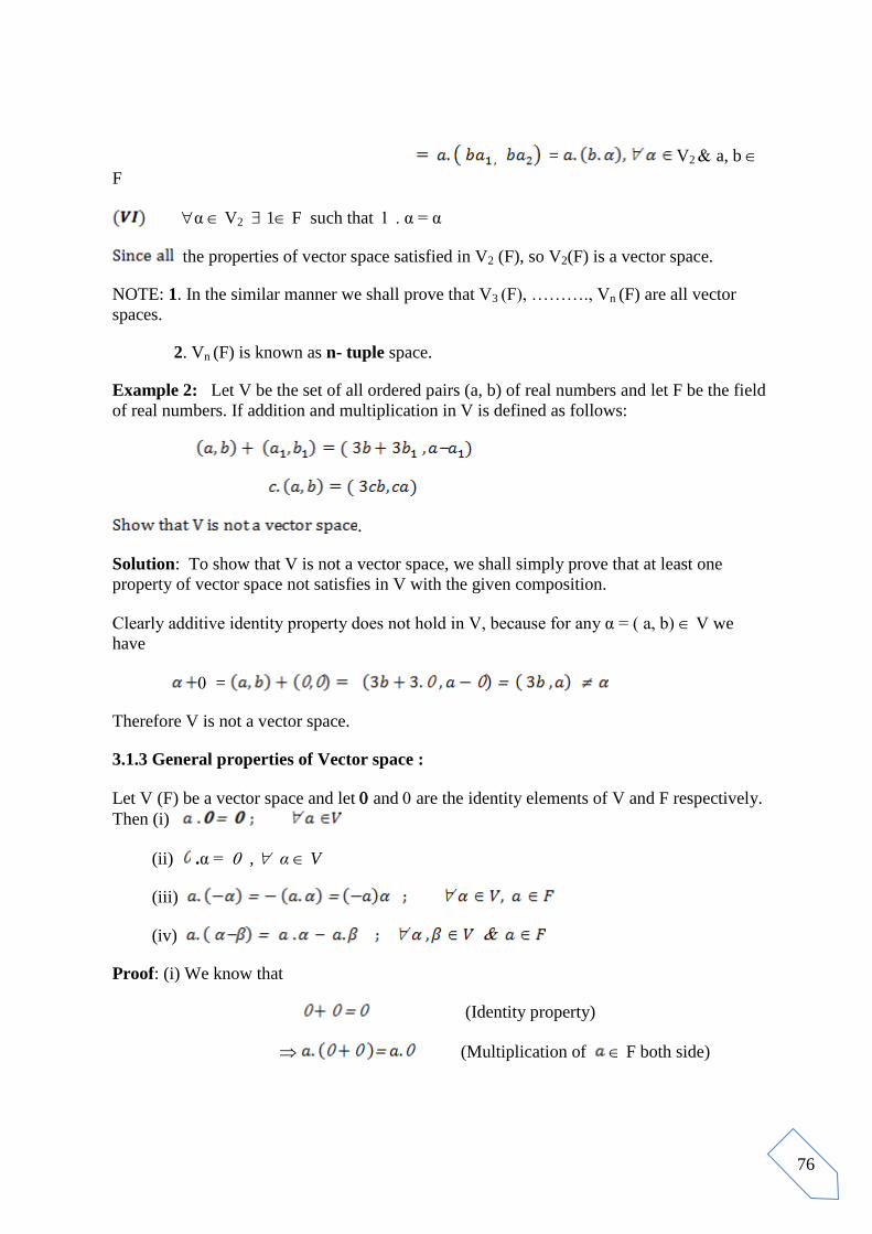
76
= V2 a, b
F
α V2 1 F such that . α = α
the properties of vector space satisfied in V2 (F), so V2(F) is a vector space.
NOTE: 1. In the similar manner we shall prove that V3 (F), ………., Vn (F) are all vector
spaces.
2. Vn (F) is known as n- tuple space.
Example 2: Let V be the set of all ordered pairs (a, b) of real numbers and let F be the field
of real numbers. If addition and multiplication in V is defined as follows:
.
Solution: To show that V is not a vector space, we shall simply prove that at least one
property of vector space not satisfies in V with the given composition.
Clearly additive identity property does not hold in V, because for any α = ( a, b) V we
have
=
Therefore V is not a vector space.
3.1.3 General properties of Vector space :
Let V (F) be a vector space and let and are the identity elements of V and F respectively.
Then (i)
(ii) .α = , α V
(iii)
(iv)
Proof: (i) We know that
(Identity property)
(Multiplication of F both side)

77
(By distributive law)
(Cancellation law)
(ii) We know that
(Identity property)
.α (Multiplication of α V both side)
(Distribution law)
(Cancellation law)
(iii) Let α V and a F , then
(Additive inverse property)
(Multiplication of a F both side)
(Distribution law)
(Additive inverse property)
Similarly we will show that .
(iv) We have
= (Distribution law)
= (By [iii])
3.2 Subspaces and algebra of subspaces :
3.2.1 Definition of Vector subspace : Let V(F) be a vector space and W be a nonempty
subset , then W is called vector subspace of V , if W is itself a vector space w. r. t. the
operation of V.
NOTE : If W V then to prove that W is a subspace of V , we simply prove that W
satisfies all the properties of vector space.
3.2.2 Some Important results on subspace :
Theorem 1 The necessary and sufficient condition for a nonempty subset W of a vector
space V (F) to be a subspace of V are
78
(i)
(ii) .
Theorem 2 The necessary and sufficient condition for a nonempty subset W of a vector
space V (F) to be a subspace of V are
(i)
(ii) .
Theorem 3 The necessary and sufficient condition for a nonempty subset W of a vector
space V(F) to be a subspace of V is .
(Note: Proof of the above theorems are very similar, so we are giving here the proof of
theorem 3 and proof of rest two will left to the reader as an exercise.)
Proof: The condition is necessary:
Let W be a subspace of V. Then we have to prove that the above
condition i.e. satisfies in W.
Now W be a subspace of V W it self a vector space ( by definition) and so vector
addition and scalar multiplication must be closed in W. Therefore
And . Hence condition is necessary.
The condition is sufficient : Let W be a non empty subset of V in which the condition
…………… (I)
is holds. We have to prove that W is sub space of V. For this we shall prove that W is itself a
vector space means all the properties of vector space satisfies in W.
Now since F is a field, unit element 1 F and so on taking a = b =1 in (I) we get
, closure property satisfied in W.
Again since F is field, ε F and for 1 F F, so on taking a= -1 and b= in (I) ,we
get α W. Hence inverse property satisfied in W.
On taking a = b = in (I) , we get .α + .β W. Thus identity element belongs to W.
Also all the elements of W belongs to V, satisfying associative and commutative -
properties in V. Hence (W, +) is abelian group.
Now on taking b= in (I) we get , indicates scalar multiplication closed in W and
remaining properties of vector space are based on scalar multiplication, thus satisfied in W.
79
Hence W is itself vector space and since W V , therefore W is subspace of V(F).
THINGS TO REMEMBER: In view of the above result to prove subspace simply prove
that the condition in W.
Theorem 4 Intersection of any two subspaces of a vector space V (F) is also a subspace of
V(F).
Proof: LetW1 and W2 are the two subspaces of vector space V (F). We shall prove that
(W1 W2) is a vector subspace of V (F). For this we shall prove that
Since W1 and W2 are the two subspaces of vector space V(F) , additive identity W1 and
W2 both and therefore W1 W2 . Hence (W1 W2) is non empty.
Now let
(Since W1 and W2 are
subspaces)
( By the definition of intersection of two sets) .
Hence (W1 W2) is a vector subspace of V(F).
Theorem 5 The union of two subspaces of a vector space is a subspace if and only if one is
contained in other.
Proof: Let W1 and W2 are the two subspaces of vector space V(F). Then theorem shall be
proved in two parts.
Part I : Let subspaces one is contained in another W1 W2 or W2 W1 . Then we
have to prove that is a subspace of V (F). Now by the definition of union of two
sets we have, if
W1 W2 W2 or W2 W1 W1.
In both the cases is either equal to W1 or W2. But W1 and W2 are subspaces of
vector space V (F), hence is subspace of V(F).
Part II: In this part we assume that is a subspace of V (F) and we shall prove
that W1 W2 or W2 W1 . On the contrary we assumed that W1 W2 or W2 W1. Then
by the definition of union of two sets we have, if

80
(i) W1 W2 α W1 but α W2
(ii) W2 W1 β W2 but β W1
From (i) and (ii) we have
[ as
]
Now by ( i ) α W1 α W1 [ as W1 is a subspace, by inverse
property ]
and by closure property W1 and α W1 α+ W1 W1 , which
contradicts (ii). Similarly by taking W2 and W2 ,we get the contradiction of (i).
Therefore our assumption that W1 W2 or W2 W1 is wrong. Hence W1 W2 or W2 W1 .
3.2.3 Examples based on subspace :
Example1. Show that the set is a subspace of V3(F) .
Solution: In view of the remark let be any two arbitrary
elements of W and let c, d ε F. Now to show that , we consider here
W ( because we get similar triad of
W)
Hence W is a subspace of V3 (F) .
Example2. Show that the set is a subspace of V2(F).
Solution: In view of the remark let be any
two arbitrary elements of W and let c, d F. Now to show that , we
consider here
]
= W (because we get similar ordered pair of
W)

81
Here . Hence W is a subspace of V2 (F).
CHECK YOUR PROGRESS:
Q.1 Show that the set of all ordered n- tuples
Vn=
is a vector space over the field F.
Q. 2 Let V be the set of all ordered pairs (a ,b) of real numbers and let field be the set of real
numbers R . Show that V is not a vector space over R with the operation addition and
multiplication defined as
Q. 3 Show that the set is a subspace of V3 (F).
Q. 4 Show that the set is a subspace of
V3(R).
Q. 5 Show that the set is a subspace of
V3(R).
3.3 Linearly dependent and independent vectors : 3.3.1 Linear sum of two vector spaces: Let W1 and W2 are the two subspaces of vector
space V(F). Then their linear sum symbolically denoted by (W1 + W2) is defined as
Linear sum of two subspaces is always a subspace. The proof is obvious and therefore
it is left to the reader as an exercise.
3.3.2 Linear combination of vectors : Let V(F) be a vector space , then a vector α V is
said to be a linear combination of the vectors if scalars
, F such that
α = +
Example: Write the vector α = ( 3, 4) as a linear combination of vectors
= ( 1, -2) in V2(R).
Solution: Let two scalars F such that
α = +
(3, 4) = +
+
=

82
On comparing the coordinates we get,
and
On solving the equations we get = . Therefore vector α can be written as
linear combination in terms of vectors as
α = Ans.
3.3.3 Linear span of a set : Let V(F) be a vector space and S be a non empty subset of V.
Then the collection of all linear combinations of finite numbers of elements of S is called set
of linear span of S. The set of linear span of S is symbolically denoted by L(S).
In brief L (S) = { + }
NOTE: (1) we write α L(S) means α definitely is in the form of linear combination of
some elements of S.
(2) The set L(S); S V is a subspace of vector space V (F). To prove it, we take
two elements α, β L(S) and two scalars a, b F and showing that
SOME THEOREMS ON LINEAR SPAN OF A SET :
Theorem 1. Let W1 and W2 are two subspaces of a vector space V(F) . Then show that
W1 + W2 = L (W1 W2).
Proof . To prove the theorem we shall prove the following two condition;
(i) W1 + W2 L (W1 W2) and (ii) L (W1 W2)W1 + W2
(i) Let α W1 + W2 α = where W1 and W2
( by the definition of linear sum of two subspaces)
also by the definition of union of two sets W1 and W2
[ being linear combination of elements
of ]
α =
Clearly every element of W1 + W2 belongs to , hence W1 + W2 L (W1 W2)
.

83
(ii)We Know that if W1 and W2 are two subspaces of V(F) , then W1 + W2 is also a subspace
of V(F). Then for every element W1 we can write
W2
every element of W1 is in W1 + W2 W1 W1 + W2
Similarly every element of W2 is in W1 + W2 W2 W1 + W2 .
Therefore (W1 W2) W1 + W2 . Also we have L (W1 W2) (W1 W2) , hence (ii).
Theorem 2. If S and T are subsets of V(F), then prove the following :
(i) S T L(S) L(T) ;
(ii) S L(T) L(S) L(T) ;
(iii) S is a subspace of V(F) L(S)= S;
(iv) L(ST) = L(S) + L(T) ;
(v) L{L(S)} = L(S) .
Proof : (i) Let α L(S) α = + L(S); where α‟s S
But S T , therefore α‟s T and so
α = + L(T).
hence L(S) L(T) .
(ii) Proof of (ii) is similar to (i), thus left to the reader as practice.
(iii) We shall prove this in two parts :
Part I : Let S is a subspace of V(F) vector addition and scalar multiplication is
closed in S and so for some vectors and scalars ,
F we have
+ S ………….(A)
On the other hand by the definition of linear span of a set we claim that
+ L(S) …………(B)
So in view of (A) and (B) we have L(S) S . Also we know that S L(S) is always true,
therefore L(S)= S.
Part II : Let L(S) = S , then we shall prove that S is a subspace of V(F). We know that L(S)
is a subspace of V(F) and L(S) = S , so S is a subspace of V(F).
(iv) Let α L(ST). Then α is a linear combination of finite elements of S and T. Let
α = + +
where S and T and a‟s and b‟s are scalars,
Now , + L(S)
and + L(T) [by the definition of linear span of a set]
Therefore

84
+ + L(S) + L(T);
[by the definition of linear sum of two subspaces]
Thus L(ST) L(S) + L(T) …..(1)
Converse part : Let = α + β L(S) + L(T) α L(S) and β L(T)
Now α L(S) α is a linear combination of finite elements of S .
Similarly β L(T) β is a linear combination of finite elements of T.
Also , S (ST) and T (ST) α + β is a linear combination of finite elements of
(ST).
Thus α + β L (ST) and consequently L(S) + L(T) L (ST) ……(2)
Hence from (1) and (2) we have L(S) + L(T) = L (ST) .
(v) We know that if S is a subspace of V (F) , then L(S)= S ; [ by (iii)]
Also L( S) is a subspace of V(F), then L{L( S)}= L( S) ; [ by (iii)] .
CHECK YOUR PROGRESS:
Q. 1 Is the vector α = (4, 2,-1) V3(R) is a linear combination of the vectors
= ( 1, -2,-1) and = ( 0, 1,-2).
Q. 2 Express the vector α = (1, 2, 5) as a linear combination of the vectors
= (1, -2,-1) and = (2,-1,1).
3.3.4 Linearly dependent vectors:
Let V (F) be a vector space and let S = { } is a subset of V(F).
Then the vectors are said to be linearly dependent if scalars
F not all zero ( some of them may be zero) such that
+ .
3.3.5 Linearly independent vectors:
Let V (F) be a vector space and let S = { } is a subset of V(F).
Then the vectors are said to be linearly independent if scalars
F, such that
+ .
.
3.3.6 Properties of Linearly dependent and independent vectors:
(I) If two vectors are linearly dependent then they are scalar multiple to each other.

85
Proof: Let α and β are two linearly dependent vectors of V(F), then two scalars a, b F (
not all zero) such that
β = ( ) α , b 0
β is a scalar multiple of α.
Similarly we shall prove that α is a scalar multiple of β.
(II) Every singleton set containing non- zero vector are linearly independent.
Proof: Let α is the only non zero vector in a singleton set S , α 0. Let scalar
aF such that
(α 0).
So here the scalar is zero , therefore set S is linearly independent.
(III) Every superset of a linearly dependent set is linearly dependent.
Proof: Let S = { } is a linearly dependent set of vectors and let
S‟ = { } be the superset of S. Now S is linearly
dependent set , then by the definition of linearly dependent set scalars
F not all zero( some of them may be zero) such that
+ ; (say 0)
+ ; (say 0)
Which clearly implies that S‟ is linearly dependent ( As all the scalars are not zero)
(IV) Every subset of a linearly independent set is linearly independent.
Proof: Let S = { } is a linearly independent set of vectors and let
S‟= { } is a subset of S. We have to prove that S‟ is linearly independent.
On the contrary let S‟ is linearly dependent. Then by the definition of linearly dependent set
scalars F ( not all zero say 0) such that
+ + = 0
+ + , which is a linear combination of the
elements of S , where all the scalars are not zero as 0.
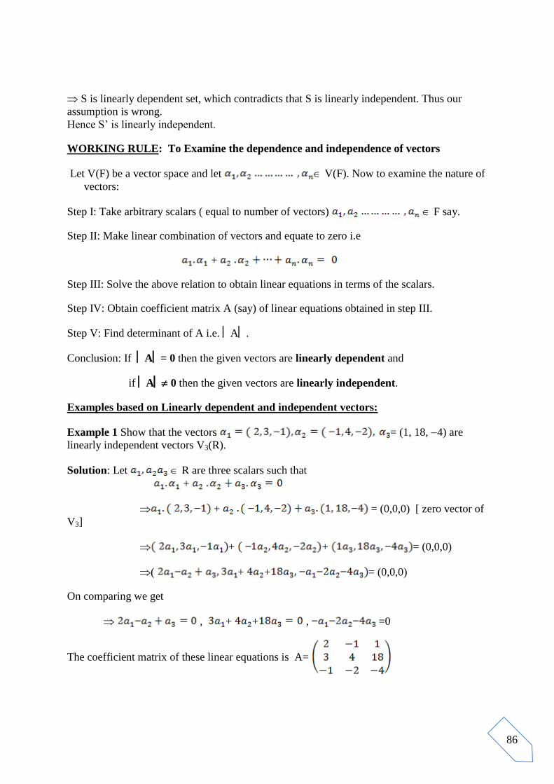
86
S is linearly dependent set, which contradicts that S is linearly independent. Thus our
assumption is wrong.
Hence S‟ is linearly independent.
WORKING RULE: To Examine the dependence and independence of vectors
Let V(F) be a vector space and let V(F). Now to examine the nature of
vectors:
Step I: Take arbitrary scalars ( equal to number of vectors) F say.
Step II: Make linear combination of vectors and equate to zero i.e
+
Step III: Solve the above relation to obtain linear equations in terms of the scalars.
Step IV: Obtain coefficient matrix A (say) of linear equations obtained in step III.
Step V: Find determinant of A i.e. A.
Conclusion: If A= 0 then the given vectors are linearly dependent and
if A 0 then the given vectors are linearly independent.
Examples based on Linearly dependent and independent vectors:
Example 1 Show that the vectors = (1, 18, 4) are
linearly independent vectors V3(R).
Solution: Let R are three scalars such that
+
+ = (0,0,0) [ zero vector of
V3]
+ + = (0,0,0)
( + + = (0,0,0)
On comparing we get
, + + , =0
The coefficient matrix of these linear equations is A=
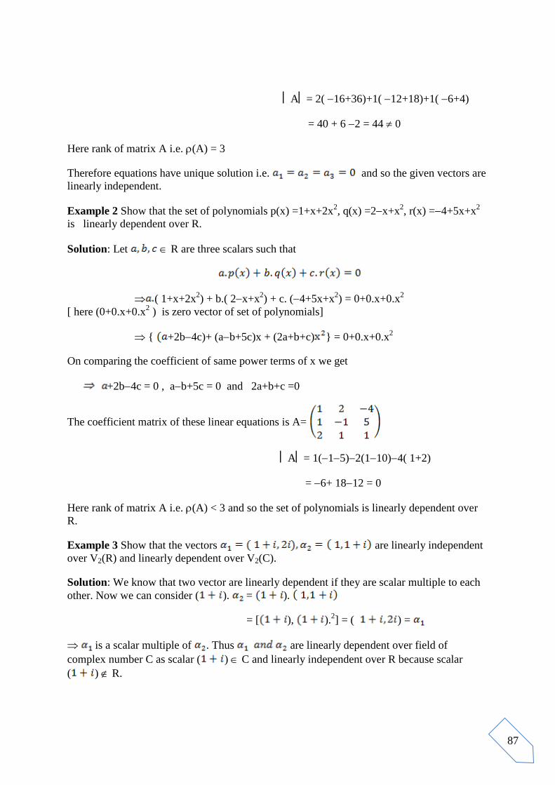
87
A= 2( 16+36)+1( 12+18)+1( 6+4)
= 40 + 6 2 = 44 0
Here rank of matrix A i.e. (A) = 3
Therefore equations have unique solution i.e. and so the given vectors are
linearly independent.
Example 2 Show that the set of polynomials p(x) =1+x+2x2, q(x) =2x+x
2, r(x) =4+5x+x
2
is linearly dependent over R.
Solution: Let R are three scalars such that
( 1+x+2x2) + b.( 2x+x
2) + c. (4+5x+x
2) = 0+0.x+0.x
2
[ here (0+0.x+0.x2 ) is zero vector of set of polynomials]
{ +2b4c)+ (ab+5c)x + (2a+b+c) } = 0+0.x+0.x2
On comparing the coefficient of same power terms of x we get
+2b4c = 0 , ab+5c = 0 and 2a+b+c =0
The coefficient matrix of these linear equations is A=
A= 1(15)2(110)4( 1+2)
= 6+ 1812 = 0
Here rank of matrix A i.e. (A) < 3 and so the set of polynomials is linearly dependent over
R.
Example 3 Show that the vectors are linearly independent
over V2(R) and linearly dependent over V2(C).
Solution: We know that two vector are linearly dependent if they are scalar multiple to each
other. Now we can consider ( ). = ).
= [ ), ).2] = ( ) =
is a scalar multiple of . Thus are linearly dependent over field of
complex number C as scalar ( ) C and linearly independent over R because scalar
( ) R.

88
Example 4 If vectors α , β , are linearly independent over V3(R), then show that vectors
α +β , β + and + α are also linearly independent over V3(R).
Solution: Let are three scalars such that
= 0
= 0 [ since α , β , are linearly
independent, all the scalars must be zero]
Thus vectors α +β , β + and + α are linearly independent over V3(R).
3.3.7 Theorems on Linearly dependent and independent vectors:
Theorem 1 Let S = { }is a subset of non zero vectors of vector space
V(F).Then set S will be linearly dependent if and only if some element of S can be expressed
as linear combination of the others.
Proof : We shall prove this theorem in two parts.
Part I: We assumed that some element of S which can be expressed as linear
combination of the others.
To prove: S will be linearly dependent. For this we shall show that at least one
scalar which is non zero in the linear combination of elements of S.
Now as per our assumption let a vector expressed as linear combination of the
others
=
+
at least one scalar
And so
Part II: We assumed that S .
To prove: some element of S can be expressed as linear combination of the others.
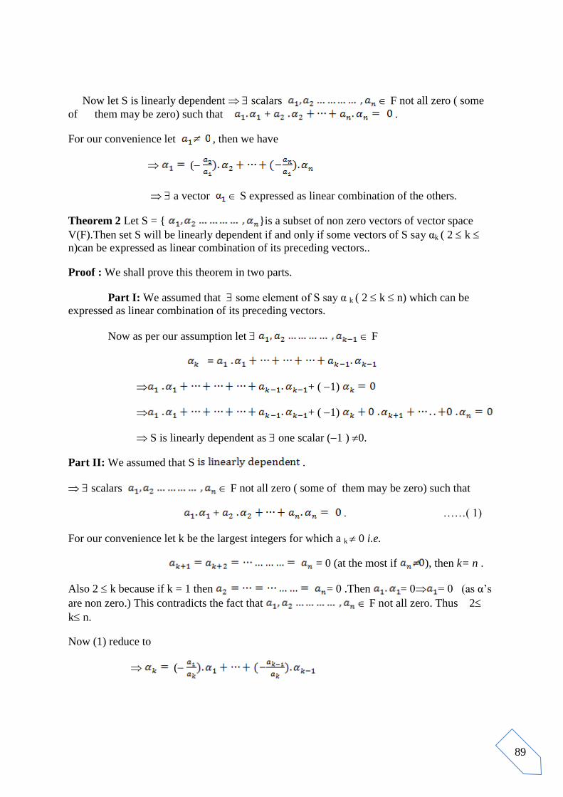
89
Now let S is linearly dependent scalars F not all zero ( some
of them may be zero) such that + .
For our convenience let , then we have
(
a vector S expressed as linear combination of the others.
Theorem 2 Let S = { }is a subset of non zero vectors of vector space
V(F).Then set S will be linearly dependent if and only if some vectors of S say αk ( 2 k
n)can be expressed as linear combination of its preceding vectors..
Proof : We shall prove this theorem in two parts.
Part I: We assumed that some element of S say α k ( 2 k n) which can be
expressed as linear combination of its preceding vectors.
Now as per our assumption let F
=
+ ( 1)
+ ( 1)
S is linearly dependent as one scalar (1 ) 0.
Part II: We assumed that S .
scalars F not all zero ( some of them may be zero) such that
+ . ……( 1)
For our convenience let k be the largest integers for which a k 0 i.e.
= 0 (at the most if ), then k= n .
Also 2 k because if k = 1 then = 0 .Then = 0 = 0 (as α‟s
are non zero.) This contradicts the fact that F not all zero. Thus 2
k n.
Now (1) reduce to
(

90
α k ( 2 k n) expressed as linear combination of its preceding vectors.
CHECK YOUR PROGRESS:
Q.1 Examine linearly dependence and independence of the following sets of vectors:
(i) = (3, 4, 7)
(ii) = (3, 1, 2)
Q.2 If vectors α , β , are linearly independent over V3(R), then show that vectors α +β , αβ
, and α2β + are also linearly independent over V3(R).
Q.3 If x, y, z are linearly independent vectors then show that the set of vectors
{x+3y-2z , 2x+2y+z, 3x- y + z}is also linearly independent.
3.4 Bases, Dimension, Finite dimensional Vector space and Related Theorems:
3.4.1 Basis of a vector space: Let V (F) be a vector space and S is a non empty subset of V.
Then S is called the basis of V (F), if:
(i) Set S is linearly independent,
(ii) S generates V (F) i.e. L(S) = V.
REMARK: (i) We know that the set of linear span i.e. L(S) is a subspace of V, therefore
L(S) V. So in order to show that L(S) = V, we simply show that V L(S).
(ii) S generates V (F) means every element of V (F) express as linear combination of the
elements of S.
3.4.2Dimension of a vector space: Let V (F) be a vector space and S = {
} is a basis of V (F), then dimension of a vector space V (F)
symbolically denoted by dimV is equal to the number of basis elements. Therefore dimV= n
(As basis S have n elements).
3.4.3 Finite Dimensional vector space: A vector space V(F) is said to be Finite Dimensional
vector space if it is generated by a finite subset of V. i.e. L(S) = V, then S must be finite.
WORKING RULE: To examine whether the given subset S of vectors of V (F) is basis or
not:
Step I: Check linear independence of set S as we discuss earlier.
Step II: Take one arbitrary element α V (F).

91
Step III: Take number of arbitrary scalars equal to the number of elements of set S.
Step IV: Put linear combination of elements of S to arbitrary element α V (F), and solve it
to find the values of the arbitrary scalars.
CONCLUSION: Set S is a basis, if set S is linearly independent and the values of the
scalars exists in the given field.
Examples based on Basis:
Example 1 Show that the set of vectors S= (1, 18, 4)}
form a basis of V3(R).
Solution: S is linearly independent: Let R are three scalars such that
+
+ = (0,0,0) [ zero vector of
V3]
+ + = (0,0,0)
( + + = (0,0,0)
On comparing we get
, + + , =0
The coefficient matrix of these linear equations is A=
A= 2( 16+36)+1( 12+18)+1( 6+4)
= 40 + 6 2 = 44 0
Here rank of matrix A i.e. (A) = 3
Therefore equations have unique solution i.e. and so the given vectors are
linearly independent.
V=L(S): For this we shall only prove that V L(S).
Let α =( a,b,c) V3 (R) be an arbitrary element and let R such that
+
+
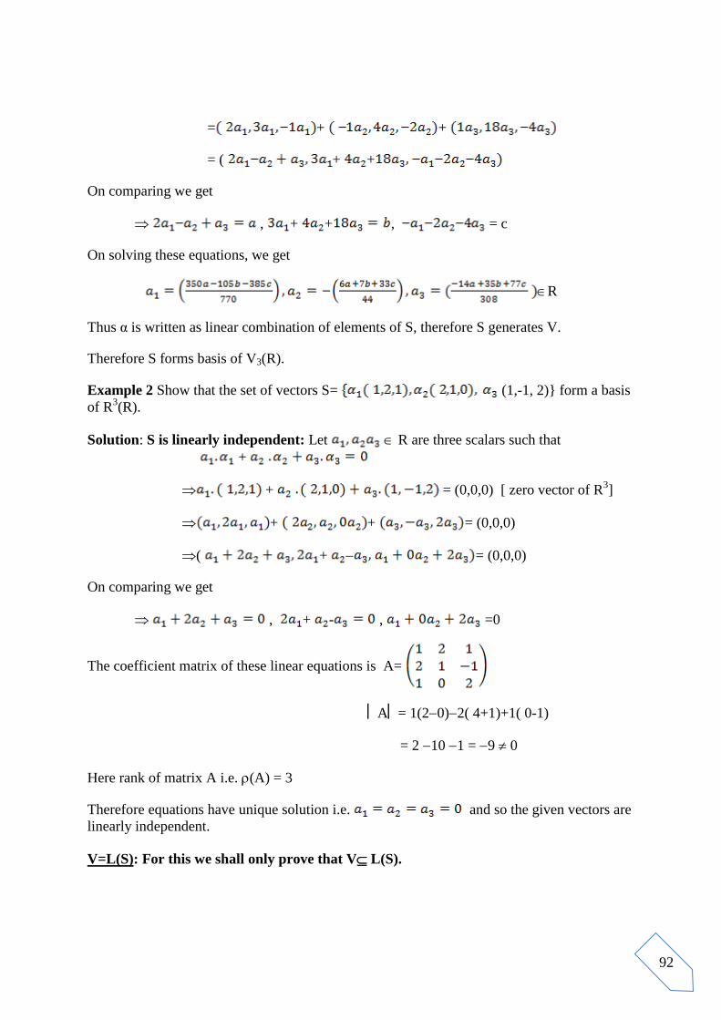
92
= + +
= ( + +
On comparing we get
, + + , = c
On solving these equations, we get
R
Thus α is written as linear combination of elements of S, therefore S generates V.
Therefore S forms basis of V3(R).
Example 2 Show that the set of vectors S= (1,-1, 2)} form a basis
of R3(R).
Solution: S is linearly independent: Let R are three scalars such that
+
+ = (0,0,0) [ zero vector of R3]
+ + = (0,0,0)
( + = (0,0,0)
On comparing we get
, + - , =0
The coefficient matrix of these linear equations is A=
A= 1(20)2( 4+1)+1( 0-1)
= 2 10 1 = 9 0
Here rank of matrix A i.e. (A) = 3
Therefore equations have unique solution i.e. and so the given vectors are
linearly independent.
V=L(S): For this we shall only prove that V L(S).
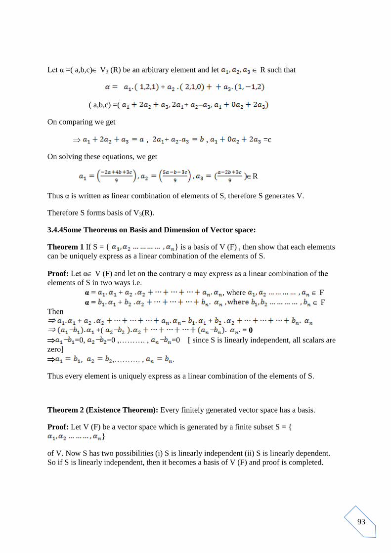
93
Let α =( a,b,c) V3 (R) be an arbitrary element and let R such that
+
( a,b,c) =( +
On comparing we get
, + - , =c
On solving these equations, we get
R
Thus α is written as linear combination of elements of S, therefore S generates V.
Therefore S forms basis of V3(R).
3.4.4Some Theorems on Basis and Dimension of Vector space:
Theorem 1 If S = { } is a basis of V (F) , then show that each elements
can be uniquely express as a linear combination of the elements of S.
Proof: Let α V (F) and let on the contrary α may express as a linear combination of the
elements of S in two ways i.e.
α = + , where F
α = + F
Then
+ = +
+( = 0
=0, =0 ,………. , =0 [ since S is linearly independent, all scalars are
zero]
, ,………. , .
Thus every element is uniquely express as a linear combination of the elements of S.
Theorem 2 (Existence Theorem): Every finitely generated vector space has a basis.
Proof: Let V (F) be a vector space which is generated by a finite subset S = {
}
of V. Now S has two possibilities (i) S is linearly independent (ii) S is linearly dependent.
So if S is linearly independent, then it becomes a basis of V (F) and proof is completed.
94
If S is linearly dependent, then some vectors of S say αk ( 2 k n)can be expressed as
linear combination of its preceding vectors [ By theorem 2 of 3.3.7]. Therefore we have
= F ….. (1)
Also as S generates V, then every element is uniquely express as a linear combination of the
elements of S. Then for any α V let
α = + , where F
……..
(2)
By (1) and (2) we have
α =
+
α is express as a linear combination of vectors .
Set S1={ } obtained by eliminating also generates V.
Again if S1 is linearly independent, it becomes basis of V and proof is completed.
On the other hand if S1 is linearly dependent, then proceeding in the same manner as above
we get a new set S2 of (n-2) elements which generates V. If S2 is linearly independent, it is
basis of V. Otherwise on continuing this process , after finite steps we get a linearly
independent set which generates V and therefore basis of V. At the most in the above process
we get a set having a single non-zero vector generating V, which is clearly linearly
independent and will become a basis.
Theorem 3 If V(F) is a finite dimensional vector space, then any two basis of V have the
same number of elements.
(This theorem is known as Invariance of the number of elements of a basis set)
Proof: Let V(F) is a finite dimensional vector space and let
S1= { }
S2={ }
be any two basis of V.
To Prove: m = n
95
Since S1 is a basis of V (F) , then each element of V can be uniquely express as a linear
combination of the elements of S1. Since V, let is uniquely express as a linear
combination of the elements of S1 as follows:
= + , where F
+ + (1) = 0
Set S3= { } is clearly linearly dependent as one scalar 1 0.
So [In view of theorem 2 of 3.3.7] a vector of Set S3 which can be express as linear
combination of its preceding vectors . If we omit from S3 then the
remaining set say
S4 = { }
generates V [as shown in the previous Theorem]. Again since V and S4 generates V, is
uniquely express as a linear combination of the elements of S4.Consequently the set
S4 = { }
is linearly dependent. Now on continuing in the same manner , each step consists in the
inclusion of a β‟s and the exclusion of a α‟s and the obtaining set generates V. Obviously the
set S1 of α‟s can not exhausted before the set S2of β‟s otherwise V(F) by a subset of S2 and S2
become linearly dependent contradicting the linear independence of S2. Hence n m.
Similarly by interchanging the role of α and β , we come to the conclusion that m n and
hence m = n.
Some useful result on basis:
1. Every set of (n+1) or more vectors in an n-dimensional vector space V(F) is linearly
dependent.
2. If V(F) is a finite dimensional vector space of dimension n, then any set of n linearly
independent vectors in V forms a basis of V.
3. If a sets S of n vectors of a finite n-dimensional vector space V(F) generates V(F),
then S is a basis of V(F).
4. If V(F) is a finitely generated vector space, then every linearly independent subset of
V is either a basis of V or extended to form a basis of V(F).( This result is known as
Extension theorem)
5. ( Dimension of a subspace) If V(F) is a finite n-dimensional vector space and if W be
a subspace of V(F), then dim W dim V. Also V= W iff dim V= dim W.

96
Proof 5: Since V(F) is a finite n-dimensional vector space and W be a subspace of V(F),
then W is also finite dimensional. Let dim W= m (say).
Now we know that (in view of result 1 above) every subset having (n+1) or more vectors
are linearly dependent, therefore W contains at most n linearly independent vectors. Let
W consists maximum m linearly independent vectors. Let S= { } be the
set consisting m linearly independent vectors where m n.
Now let α W is an arbitrary element, then as per our assumption set S1=
{ }
consisting (m+1) vectors is linearly dependent and can not be a basis of W . Therefore
dim W = m n = dim V i.e. dim W dim V
Also if subspace W has a basis set consisting n element, then this particular basis set of n
linearly independent vectors is a subset of V and hence form a basis of V.( In view os
above result 2) . And so V= W iff dim V= dim W.
CHECK YOUR PROGRESS:
Q.1 Show that the set of vectors S= (0,0,1)} form a basis of
R3(R).
Q.2 Examine whether the vectors (3,1,-2) form a basis of V3(R)
or not.
Q.3 If the set of vectors S= { α, β, }form a basis of V3(R) , then show that the set of vectors
S1={ α + β, β + , + α} also form a basis of V3(R).
Q.4 Prove that the set of vectors S = { } is a basis set of C(R) if
Hint: Let x ,y R such that
x.( )+y.( ) = 0
(a.x + y.c) + ( b.x + d.y) = 0+ [ zero vector of set of complex number
C]
a.x + y.c = 0 and b.x + d.y= 0 [ on comparing real & imaginary part]
We know that set is linearly independent if 0
Again let α = C is arbitrary element, then

97
( ) = x.( )+y.( )
On solving, we get x = , y = R, if
Q.5 Show that the set of vectors S= (0, 1, 0), (1, 1, 1)} is not a basis of
V3(R).
3.5 Dimensions of Sums of Subspaces, Quotient Space and its Dimension:
3.5.1 Quotient Space: Let V(F) be a vector space and W be a subspace of V. Then the
quotient space is the set of all right(or left) cosets of W in V i.e.
V/W = {W + α : α V}.
Vector addition and scalar multiplication in V/W is defined as below:
Vector addition (W+ α) + (W + β) = W + (α + β) ; (W+ α) , (W + β) V/W
Scalar multiplication a. (W+ α) = W+ a. α ; (W+ α) V/W and a F
NOTE: 1. Elements of Quotient space are always taken in the form of cosets (right or left).
2. Zero vector of quotient space V/W is taken as (W+0) or W.
3. Additive inverse of any element (W + α) is [W +(- α)].
4. By cosets property, we have W + α = W + β (αβ) W.
3.5.2 Theorem based on Dimension of Quotient Space and Sums of Subspaces:
Theorem 1 Let V (F) be a finite dimensional vector space and W be a subspace of V. Then
dim V/W = dim V dim W.
Proof: Let dim W= m, then basis of W consists m elements. Let S1= { } be
a basis of W. Now since W be a subspace of V, then S1 V is linearly independent set being
basis. So by extension theorem, we can obtain a basis of V by extending set S1. Let
S2= { }
be a basis of V. Then dim V = m+ n.
Now in order to prove the theorem, we shall prove that dim V/W = (m+ n) m = n.
It means we claim that basis of quotient space V/W consists n elements. For this let
98
S= { }
is a subset of V/W having m elements. To prove that S forms a basis of V/W, we shall first
show that :
(i) S is linearly independent: Let F such that
[W+0 is zero vector of
V/W]
W+ ( ) = W+ 0
W [Note 4]
Now since S1= { } be a basis of W, therefore every element of W can be
written as a linear combination of the element of S1, and so
W.
Thus such that
=
+ ( = 0
(Because are basis elements of V and so they are linearly
independent)
, hence S is linearly independent.
Now we shall prove that
(ii) V/W = L(S): Let (W+ α) V/W be an arbitrary element, where α V.
Since S2= { } is basis of V, we can express α as a linear
combination of the element of S2. Let
α = + ,
[where a‟s and b‟s are scalars]
W+ α = +
W+ α = +
Here as
W
[by cosets property W+ α = W α W]
Therefore W+ α =
(W+ α) written as a linear combination of the element of S, hence V/W = L(S).
S is a basis of V/W and dim V/W = n.
99
Therefore dim V/W = dim V dim W.
Theorem 2 Let V (F) be a finite dimensional vector space and let W1 and W2 are two
subspaces of V(F). Then prove that
dim ( W1 + W2) = dim W1 + dim W2 dim ( W1 ∩ W2) .
[ This theorem is known as Dimension of Linear Sums of Subspaces of a vector space.]
Proof: Let dim (W1 ∩ W2) = k , then basis of ( W1 ∩ W2) having k elements. So let
S1= { } be a basis of (W1 ∩ W2). Also we know that ( W1 ∩ W2) W1 and
(W1 ∩ W2) W2, therefore S1 W1 and S1 W2. Since S1 is linearly independent set , can be
extended to get the bases of W1 and W2.
Let S2 = { } and
S3={ } are the basis of W1 and W2 respectively.
Clearly dim W1 = k+ l and dim W2 = k+ m , therefore
dim W1 + dim W2 dim ( W1 ∩ W2)= (k+ l ) + (k+ m) k
= k + l + m .
In order to prove the theorem we shall prove that dim (W1 + W2) = k + l + m.
For this it is sufficient to show that the a set having (k + l + m) elements forms a basis of
(W1+ W2) . Let S = { } having (k + l + m)
elements.
Our claim: S is a basis of (W1+ W2). First we show that,
(I) S is linearly independent:
Let scalars F such that
………(1)
…….(2)
Since ‟s and α‟s are the basis elements of W1 therefore W1
And so W1
…….(3)
But are the part of basis of W2, then
W2 [being subspace]
….(4)
, we have

100
(W1 ∩ W2)
Now since { } be a basis of (W1 ∩ W2), we write
as linear combination of basis elements. So let F such that
( since β‟s and ‟s are linearly
independent vectors)
Then by (1) ,we have = 0
( since α‟s and ‟s are
linearly independent vectors)
Finally we get
Hence S = { } is linearly independent.
(II) S generates (W1+ W2) : Let α W1 and β W2 α + β (W1+ W2) [ By the definition
of linear sum of subspaces].
Now α W1, express as linear combination of basis of W1. Let scalars
F such that
α =
……..(5)
Similarly β W2, express as linear combination of basis of W2. Let scalars
F such that
β =
……..(6)
On adding (5) and (6) we get
α +β = +
( )

101
= +
Hence S generates W1+W2.
3.5.3 Co-ordinate representation of a vector: Let V (F) be a finite dimensional vector space
of dimension n. Let S = be a ordered basis of V (F). Then for each αV
a unique set of scalars F (say), by which we can express α as a linear
combination. This set of scalars { } is called the co-ordinate of vector α
related to the ordered basis S.
NOTE: Ordered basis means a basis in which the order of elements are fixed. The co-
ordinate of a vector may change with change in the order of elements of basis.
Example 1 Find the co-ordinate of vector α= (3, 1,4) relative to basis S={(1,1,1), (0,1,1),
(0,0,1)}of V3 (R).
Solution: To find the co-ordinate of a vector, we simply find the scalars by which we can
express the given vector, as linear combination. So let scalars are R such that
α =
(3, 1,4) = (0,0,1)
=
On comparing, we get
, ,
Therefore co-ordinate representation of vector α relative to the basis S is (3,-2,-5).
Symbolically we write as S = (3,-2,-5).
CHECK YOUR PROGRESS:
Q. 1 Find the co-ordinate of vector α relative to the basis S= = {(1, 1, 1), (0, 1, 1), (0, 0, 1)}
of V3 (R), where
(i) α = (4, -3, 2)
(ii) α = (a, b, c).
Q. 2 Find the co-ordinate of vector α = (2, -1, 6) relative to the basis S= {(1, 1, 2), (3, 1, 0),
102
(2, 0, -1)} of V3 (R).
POINTS FOR DISCUSSION/ CLARIFICATION:
After going through the unit you may like to seek discussion/ clarification on some points. If
so, mention these points below:
(I) Points for Discussion:
(II) Points for Clarification:
REFERENCES:
1. Linear Algebra, Kenneth Hoffman and Ray Kunz, Prentice-Hall Inc.
2. Algebra, M. Artin, Prentice-Hall of India Pvt. Ltd., New Delhi
3. Introduction to Modern Algebra, Neal H. Macoy, Bostan, Allay & Bacon, Inc.
4. Linear Algebra: Ideas and Application, Richard C. Penney, Wiley Inter-Science, A
John Wiley and Sons. Inc. Publication
103
UNIT – IV
LINEAR TRANSFORATION
Structure:
4.1 Linear Transformation and Their Matrix Representation
4.2 Algebra of Linear transformations
4.3 The Rank Nullity Theorem
4.4 Change of Basis, Dual and Bidual Space, Natural Isomorphism
4.5 Adjoint of a Linear transformation
4.6 Eigen values, Eigen vectors of a Linear transformation, Diagonalisation
4.7 Bilinear, Quadratic and Hermitian Forms.
*Points for Discussion/ Clarification
**References
4.1 Linear Transformation and Their Matrix Representation:
4.1.1 Definition of Linear Transformation: Let U (F) and V (F) be two vector spaces. Then
a mapping f defined from U (F) to V (F) (symbolically written as f :U V) is called Linear
Transformation or Linear Map or Homomorphism on vector space if the following
conditions are satisfied:
(I) f ( + ) = f ( ) + f (), , U
(II) f ( a.) = a. f ( ), U a F
Or
, U and a,b F
NOTE: To prove that the given mapping (in a question) is a linear map, we simply prove the
above stated conditions (I) and (II) or the combined condition holds.
For Example: (1) Show that the mapping defined by is
a linear map.
Solution: Let and a, b R, then we have
= and = ….
(1)
Now,
= , where
= , [by the definition of f]
= , [on putting the value of x and
y]
= [write the terms of a and b
together]
=
= [by (1)]
Therefore is a linear map.

104
Example (2): Show that the mapping defined by
is a linear map.
Solution: Let and a ,b R, then we have
= and = ….
(1)
Now,
=
=
= [( ) ) , ( )( )] …
(2)
(By the definition of
f )
Now
= , [by (1)]
=
=
= [( ) ) , ( )( )] …
(3)
So by (2) and (3), we have
Therefore mapping is a linear map.
4.1.2 Properties of Linear Map:
If f : U(F) V(F) is a linear map. Let 0 and 0’ are zero vectors of U and V
respectively, then we have:
(I)
(II) , U
(III) , , U
Proof: (I) We know that for any U and 0 U,
+ 0 =
,
+ = , [as f is a linear map]
+ = , [as 0’ is zero vector of V]
, [by left cancellation law]
(II) We know that for any U U such that
+() = 0
+ = , [as f is a linear map]
+ = , [as ]
105
= , [additive inverse property]
(III) We know that
= , [by (II)]
4.1.3 Definition of Kernel of a Homomorphism (Linear map): Let U (F) and V (F) be two
vector spaces. Let f : U(F) V(F) is a linear map (homomorphism), then the set K of all
those elements of U (F) whose image under f are zero element of V (F), is called Kernel of
a Homomorphism f (Linear map f). It is also denoted by Ker f or
THINGS TO REMEMBER:
(1) If .
(2) To prove that any element, say , we simply show that the image of under
mapping f are zero element of V (F) i.e. .
(3) Let f : U(F) V(F) is a linear map (vector space homomorphism), then Ker f or is a
subspace of U (F).
To prove this we take two elements (say) , and two scalars a, b F and show that
or in view of note (2) above, we shall prove that . Now
…. (1)
Therefore,
= [by (1)]
Ker f or is a subspace of U (F).
(4) A mapping f : U(F) V(F) is called one-one mapping if distinct elements of U have
distinct images in V. To prove that a given mapping is one-one, we simply consider the
images of two elements are equal and show that elements are also equal i.e. if , U are
such that
= .
(5) A mapping f : U(F) V(F) is called onto mapping if every element of V is engaged with
at least one element of U. To prove that a given mapping is onto, we simply consider one
arbitrary element V and for this we find one element U in such a way that relation
holds.
4.1.4 Isomorphism of Vector Spaces: Let U (F) and V (F) be two vector spaces. Then a
mapping f : U(F) V(F) is a called isomorphism, if
(I) Mapping f is one-one.
(II) Mapping f is onto.
(III) Mapping f is homomorphism
And in this case vector spaces U (F) is called isomorphic to V (F) and denoted symbolically
by
U(F) V(F). In other words V (F) is called isomorphic image of U (F).
Solved Examples on Isomorphism of Vector Spaces:
Example 1 Show that the mapping defined by is an
isomorphism.

106
Solution: Let and a, b R, then
(I) Mapping f is one-one: Let
,
, [by the definition of f ]
.
Mapping f is one-one
(II) Mapping f is onto: Let is an arbitrary element. Now
Such that .
Every element of is engaged with at least one element of .[since is
arbitrary]
Mapping f is onto.
(III) Mapping f is homomorphism: Let and a, b R,
then
= , where
= , [by the definition of f]
= , [on putting the value of x and y]
= [write the terms of a and b together]
=
= [by the definition of f]
= Mapping f is homomorphism.
In virtue of (I), (II) and (III) is an isomorphism.
Example 2 Find the kernel i.e. defined by
.
Solution: By the definition of kernel i.e. , we simply find those
elements of whose images are zero vector i.e. (0,0) in . For this, we assume that
there is an arbitrary element = such that
, [zero vector of ]
,
Elements of whose images is zero vector in are of the form = .
Therefore, Ker f i.e. = { : c R}.
CHECK YOUR PROGRESS:
Q. 1 Show that the mapping defined by is a linear
map.

107
Q. 2 Show that the mapping defined by is a
linear map.
Q. 3 Show that the mapping defined by
is an isomorphism.
Q. 4 Let C (R) be the vector space of all complex numbers over the field R. Then show that
the mapping T (a +i b) = (a, b) is an isomorphism.
4.1.5 Some Results on Isomorphism of Vector Spaces:
Theorem 1: Two finite dimensional vector spaces over the same field are isomorphic if and
only if their dimensions are same.
Proof: Part I: Let U (F) and V (F) be two finite dimensional vector spaces, then let
dim U = dim V= n (finite)
Let S = { } and S‟ = { } are the bases of U and V respectively.
To Prove: U V, we shall define a mapping f : U(F) V(F) as below:
Where = U (F), and show that f is one-one, onto and linear.
(Detailed proof is left to the reader as an exercise.)
Part II: Let U V a mapping f : U(F) V(F) which is isomorphic.
To Prove: dim U = dim V.
For this let dim U = n and let S = { } is the basis of U (F).
Then to prove the theorem, we claim that the set of images of the elements of S i.e.
S‟= { } forms a basis for V (F). For this show that S‟ is linearly
independent and it generates V.
(Detailed proof is left to the reader as an exercise.).
Theorem 2: Every n-dimensional vector space V (F) is isomorphic to Vn(F).
Proof: Given: V (F) is a n-dimensional vector space. Clearly basis of V (F) contains n
elements.
Let S = { } is the basis of V (F). Therefore S generates V, and so every
element of V expressed as linear combination of the elements of S. If V, then scalars
F such that
= ,
Again if F ) Vn(F).
Thus to prove that V(F) Vn(F) , we shall define a mapping (say) f : V(F) Vn(F) as
) , where = .
And show that f is one-one, onto and linear.
(I) f is one-one: Let , V and let = .
Now let,
) = ) [by the definition of f ]
[as
]
, hence f is one-one .
(II) f is onto: Let ) Vn(F).
an element = V(F) such that )
.
108
Therefore f is onto .
(III) f is linear: Let , V and let F. Now
=
f
= [ ], [by the definition of f ]
= ) + ) =
Mapping f is homomorphism.
Hence is an isomorphism.
4.1.6 Matrix Representation of a Linear Map:
Let U (F) and V (F) be two finite dimensional vector spaces and T: U(F) V(F) is a linear
map. Let S = { } and S‟ = { } are the bases of U and V
respectively. Then to obtain required matrix representation of T, we go through the following
steps:
Step I: Find the images of basis elements of U i.e. T( ), T( ),. . . , T( ).
Step II: Write each image T( ), k=1,2…,n as linear combination of the basis elements
of V(F), by taking arbitrary scalars i.e.
T( ) = }, k=1,2…,n
Step III: Find the values of the unknown scalars by solving the
system of equations.
Step IV: Obtained co-efficient matrix i.e.
Step V: Transpose of the above matrix is required matrix representation of T.
Symbolically it is written as [ T ; S ; S‟].
NOTE: (1) Notation [ T ; S ; S‟] indicates the matrix representation of linear map T
with respect to the bases S and S‟.
(2) If bases of vector spaces are not given, then we use natural bases of concerning
vector spaces.
(3) If a linear map is defined in the same spaces, then basis S and S‟ are same.
Solved Examples on Matrix Representation of a Linear Map:
Example 1 If T: R3 R
3 be a linear map defined by ,
T ( ) = ( ).
Determine the matrix relative to the ordered basis { }.
Solution: Here S ={ }= S‟ [ Note (3)]
Images of basis elements:
T ( ) = T = ( 1+1+1 , 114 , 21),
[Here By the definition of
T]
T ( ) = (3, 6, 1)
Similarly T ( ) = T = (2, 5, 1) and T ( ) = T = (2, 5, 1), [Step I]

109
Now let scalars F such that
T ( ) = , [Step II]
On substituting the values, we get
(3, 6, 1) =
= ( )
On comparing both sides, we get
On solving, we get
[Step
III]
Similarly, after expressing T ( ) and T ( ) as linear combination and solving we get
And
Here coefficient matrix is [Step
IV]
Now transpose of the above matrix, gives required result i.e.
Required matrix representation of T i.e. [T; S; S‟] = [Step
V]
Example 2 If T: R2 R
2 be a linear map defined by,
T ( ) = (2y, 3x y).
Determine the matrix relative to the ordered basis { }.
Solution: Here S= { }.= S‟ [ Note
(3)]
Images of basis elements:
T ( ) = T = [2(3), 3(1)3], [Step I]
[Here By the definition of T]
T ( ) = (6, 0)
Similarly T ( ) = T }= ( 2(5) , 3(2)3) = (10 , 1) [ Step I]
Now let scalars F such that
T ( ) = , [Step II]
On substituting the values, we get
(6, 0) =
= ( )
On comparing both sides, we get
On solving, we get
[Step III]

110
Similarly, after expressing T ( ) as linear combination and solving we get
Here coefficient matrix is [Step IV]
Now transpose of the above matrix, gives required result i.e.
Required matrix representation of T i.e. [T; S; S‟] = [Step V] Ans.
CHECK YOUR PROGRESS:
Q.1 If T: R3 R
2 be a linear map defined by ,
T ( ) = ( ).
Determine the matrix relative to the usual bases.
(Hint: Usual bases of R2 and R
3 are {(1,0), (0, 1)}and{(1,0,0), (0,1,0), (0,0,1)})
Ans.
.
Q. 2 If T: R2 R
2 be a linear map defined by, T ( ) = (4x2y, 2x + y).
Determine the matrix relative to the ordered basis { }.
Ans. .
Q. 3 Find the matrix representation of a linear map T : V3 (R) V3 (R), defined by
T (a, b, c) = (a b, b a, a c),
Relative to the basis S = { .
Ans.
.
4.2 Algebra of Linear Transformation:
4.2.1 Some useful Results on Linear Transformation:
(I) Let is a linear mapping. Then f is one-one if and only if Ker f = {0}.
Proof: Part I: Let Ker f = {0}, then we shall prove f is one-one. Let , U are such that
[Additive inverse property]
[By the properties of linear map]
Ker f [By the definition of Ker f]
[Since Ker f = {0}]
f is one-one.
Part II: Let f is one-one. We shall prove that Ker f = {0}.Means Ker f has only one element
i.e. 0.
Let us take an arbitrary element Ker f , then by the definition of Ker f , we have
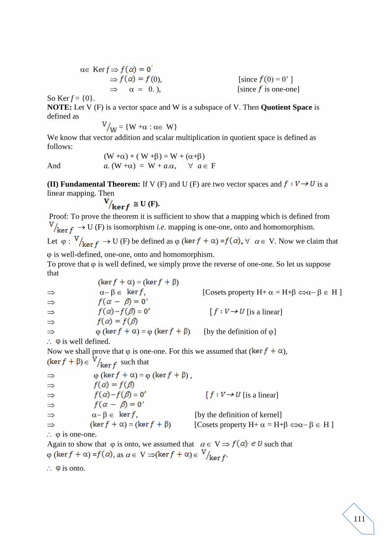
111
Ker f
0), [since 0) = 0‟ ]
0. ), [since is one-one]
So Ker f = {0}.
NOTE: Let V (F) is a vector space and W is a subspace of V. Then Quotient Space is
defined as
= {W + : W}
We know that vector addition and scalar multiplication in quotient space is defined as
follows:
(W +) + ( W +) = W + (+)
And a. (W +) = W + a., a F
(II) Fundamental Theorem: If V (F) and U (F) are two vector spaces and is a
linear mapping. Then
U (F).
Proof: To prove the theorem it is sufficient to show that a mapping which is defined from
U (F) is isomorphism i.e. mapping is one-one, onto and homomorphism.
Let : U (F) be defined as ( ) = , V. Now we claim that
is well-defined, one-one, onto and homomorphism.
To prove that is well defined, we simply prove the reverse of one-one. So let us suppose
that
( ) = ( )
, [Cosets property H+ = H+ H ]
= [is a linear]
( ) = ( ) [by the definition of ]
is well defined.
Now we shall prove that is one-one. For this we assumed that ( ),
( ) such that
( ) = ( ) ,
= [is a linear]
, [by the definition of kernel]
( ) = ( ) [Cosets property H+ = H+ H ]
is one-one.
Again to show that is onto, we assumed that V such that
( ) = , as V ( ) .
is onto.
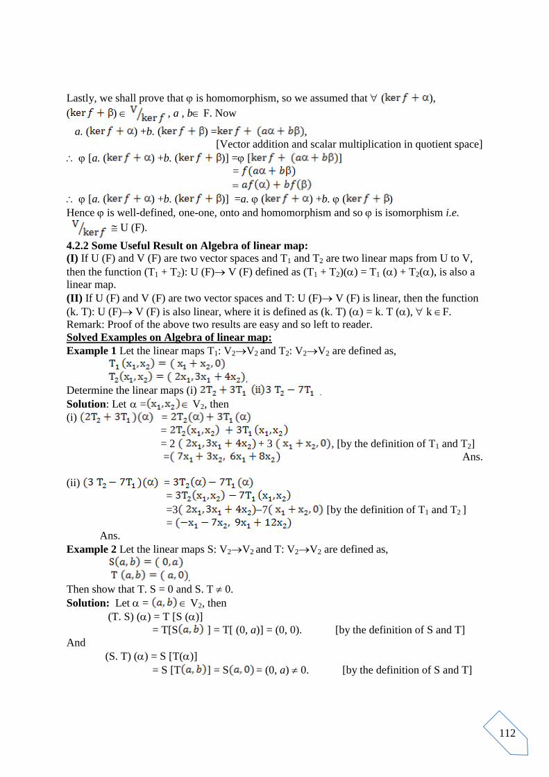
112
Lastly, we shall prove that is homomorphism, so we assumed that ( ),
( ) , a , b F. Now
a. ( ) +b. ( ) = ,
[Vector addition and scalar multiplication in quotient space]
[a. ( ) +b. ( )] = [ ]
=
[a. ( ) +b. ( )] =a. ( ) +b. ( )
Hence is well-defined, one-one, onto and homomorphism and so is isomorphism i.e.
U (F).
4.2.2 Some Useful Result on Algebra of linear map:
(I) If U (F) and V (F) are two vector spaces and T1 and T2 are two linear maps from U to V,
then the function (T1 + T2): U (F) V (F) defined as (T1 + T2)() = T1 () + T2(), is also a
linear map.
(II) If U (F) and V (F) are two vector spaces and T: U (F) V (F) is linear, then the function
(k. T): U (F) V (F) is also linear, where it is defined as (k. T) () = k. T (), k F.
Remark: Proof of the above two results are easy and so left to reader.
Solved Examples on Algebra of linear map:
Example 1 Let the linear maps T1: V2V2 and T2: V2V2 are defined as,
,
Determine the linear maps (i) .
Solution: Let = V2, then
(i) =
=
= 2 + 3 , [by the definition of T1 and T2]
= Ans.
(ii) =
=
=3 7 [by the definition of T1 and T2 ]
=
Ans.
Example 2 Let the linear maps S: V2V2 and T: V2V2 are defined as,
,
Then show that T. S = 0 and S. T 0.
Solution: Let = V2, then
(T. S) () = T [S ()]
= T[S ] = T[ (0, a)] = (0, 0). [by the definition of S and T]
And
(S. T) () = S [T()]
= S [T ] = S = (0, a) 0. [by the definition of S and T]

113
4.2.3 Invertible (Non Singular) Linear Map:
If U (F) and V (F) are two vector spaces and T: U (F) V (F) is linear map
(transformation) is called non singular or invertible if
T () = 0’ = 0, U.
WORKING RULE TO SHOW A GIVEN MAPPING IS INVERTIBLE:
Let T: U (F) V (F) is linear map, then
Step I: Take an arbitrary element U.
Step II: Put its image equal to zero vector of V i.e. T () = 0‟
Step III: Apply the definition of T and solve.
Conclusion: If = 0, then T is invertible.
Solved Example on Invertible (Non Singular) Linear Map:
Example 1 Let T: V2V2 be a linear maps over the field F and it is defined as
,
Show that T is invertible and find the formula for T 1
.
Solution: Let = V2 and let
T () = 0‟
[0‟ = (0, 0)is zero vector of V2]
= , [definition of T]
,
= , so T is invertible.
Formula for T 1
: Let = V2 such that
T 1
()
T 1
….. (1)
T =
=
We get here, and . So, by (1) we have
T 1
( ). Ans.
Example 2 Let T: V3V3 be a linear map over the field F and it is defined as
, + , + ,
Show that T is invertible and find the formula for T 1
.
Solution: We know that { = (0, 1, 0), } is natural basis of V3
and so we can express every element of V3 as a linear combination of basis elements.
Therefore for any = (x, y, z) V3, let scalars such that
=
(x, y, z) =
=
T () = )
= ), {T is linear}

114
= , {by the definition of T}
After putting the values of and on solving, we get
=
T (x, y, z) = .
Now let = (x, y, z) V3 and let
T () = 0‟
[0‟ = (0, 0, 0) is zero vector of V3]
= , [definition of T]
= so T is invertible.
Formula for T 1
: Let = V3 such that
T 1
()
T 1
(x, y, z)
T = (x, y, z)
= (x, y, z)
On solving, we get
Therefore required formula is
T 1
(x, y, z) .
CHECK YOUR PROGRESS:
Q. 1 Let the linear maps S: V2V2 and T: V2V2 are defined as, and
, Then find the maps (i) T. S (ii) S. T (iii) S + T (iv) 3S 2T.
[Ans. (i) (ii) (iii) (iv) .]
Q. 2 Let T be a linear transformation on R3 defined as
,
Then show that T is invertible and find T 1
.
[Ans. T 1
(a, b, c) =
( )]
Q. 3 Let T: V3V3 be a linear map over the field F and it is defined as
, 7 ,
Show that T is invertible and find the formula for T 1
.
[Ans. T 1
(a, b, c) =
( )]
4.3 Rank and Nullity of Linear Mapping:
4.3.1 Range of a Linear Mapping: Let U (F) and V (F) are two vector spaces and T: U V
is a linear mapping. Then range of T denoted by R (T) is the set of all images of the elements
of U (F). In brief
R (T) = {T () V: U}.
REMARK: It can be easily seen that R (T) is a subspace of V (F).

115
4.3.2 Null space of a Linear Mapping: Let U (F) and V (F) are two vector spaces and
T: U (F) V (F) is a linear mapping. Then the null space denoted by N (T) is the set of all
such elements of U whose image is zero vector in V. In brief
N (T): { U: T () = 0’}
REMARK: It can be easily seen that N (T) is a subspace of U (F). Null space is also known
as Kernel.
4.3.3 Rank of a Linear Mapping: Let U (F) and V (F) are two vector spaces and T: U V
is a linear mapping. Then rank of T denoted by ρ (T) is the dimension of the range set R (T).
Therefore Rank of T i.e.
ρ (T) = dim [R (T)].
4.3.4 Nullity of a Linear Mapping: Let U (F) and V (F) are two vector spaces and T: U V
is a linear mapping. Then nullity of T denoted by υ (T) is the dimension of the null space N
(T). Thus,
Nullity of T i.e. υ (T) = dim [N (T)].
WORKING RULE TO FIND RANK AND NULLITY:
Step I: Take the standard basis (natural basis) concerning to vector space U (F).
Step II: Find the images of basis elements which forms range space R (T).
Step III: If the obtained images are linearly independent, their number gives dim [R
(T)] . i.e ρ (T) = dim [R (T)], otherwise find number of linearly
independent images.
Step IV: Take one arbitrary element of U and put its image equal to zero vector of V.
Step V: By solving the above relation, find actual element of U (means value of
arbitrary
element).
Step VI: If the obtained element is other than zero element, gives us N (T) otherwise it
is
null.
Step VII: Number of elements in N (T) gives us dim [N (T)] i.e. υ (T) = dim [N (T)].
Solved Example on Rank and Nullity of Linear Map:
Example 1 Find the range, rank, null space and nullity of T for the given linear
transformation:
(I) T: R2 R
3 defined as
(II) T: R3 R
3 defined as
Solution (I): Consider the natural basis of i.e. { }.
Now,
T ( ) = T = T ( ) = T =
Range space is {T ( ) , T ( ) }= { }.
Since above vectors are not scalar multiple to each other, therefore they are linearly
independent. Hence, dim [R (T)] = 2.

116
Rank of T i.e ρ (T) = dim [R (T)] = 2.
Again let = be an arbitrary element such that,
T () = 0‟
[0‟ = (0, 0, 0) is zero vector for ]
= , [definition of T]
, ,
.
= , so null space N (T) = { : 0 R}.
Therefore dim [N (T)] i.e. υ (T) = dim [N (T)] = 0
Solution (II): Consider the natural basis of i.e. {
}.
Now,
T ( ) = T = T ( ) = T =
And T ( ) = T =
Range space is {T ( ), T ( ), T ( )} = {
Now to examining the linearly independence, let us assumed that scalars R such
that
( ) =
, ,
Here coefficient matrix is A = 1 (-2-1) +1(2+1) = 0
Vectors are linearly dependent. Also first two vectors are clearly linearly independent,
therefore dim [R (T)] = 2
Rank of T i.e. ρ (T) = dim [R (T)] = 2.
Now for null space, let = be an arbitrary element such that,
T () = 0‟
[0‟ = (0, 0, 0) is zero vector for ]
= , [definition of
T]
, ,
= , so null space N (T) = { }.
Therefore dim [N (T)] = 1, hence υ (T) = dim [N (T)] = 1.
4.3.5 Rank Nullity Theorem:
Let U (F) and V (F) are two vector spaces and T: U V is a linear mapping. If U (F) be
finite dimensional, then
Rank (T) + Nullity (T) = dim U.

117
Proof: We know that null space of T i.e. N (T) is subspace of U and U (F) be finite
dimensional, therefore N (T) is also finite dimensional. Let dim N (T) = k and let S‟ =
{ } be the basis of N (T).
Then by Extension theorem, we can obtain basis for U (F). So let S‟‟=
{ } be the basis of U (F). Then dim U= n.
To prove the theorem, we claim that
Rank (T) = dim U Nullity (T)
i.e. dim [R(T)] = dim U dim [N(T)]
i.e. dim [R(T)] = (n k)
For this we shall consider a subset of R (T), say S = { } and
prove that it forms a basis for R (T).
(I) S is Linearly Independent: Let scalars F such that
= 0‟
T ( ) = 0‟
N (T), [by the definition of null
space]
Since each element of N (T) can be express as a linear combination of its basis S‟, therefore
let scalars F such that
,
Because are the basis elements of S‟‟, thus they are linearly
independent.
scalars are all zero, hence S is linearly independent.
(II) S generates R (T): For this, let T () R (T) is an arbitrary element. Now we shall prove
that T () can be express as linear combination of the elements of S.
Now if T () R (T) U, [as T: U V is a linear mapping]
And if U, we write as linear combination of the basis of U. So let
= +
T () = +
= +
[As N (T) ]
S generates R (T).Thus S = { } forms a basis for R (T)
and theorem holds.
CHECK YOUR PROGRESS:
Find the range, rank, null space and nullity for the following linear transformation:
Q. 1 T: V2 V3 defined as 2.
[Ans. R (T) = {(1, 1, 0), (1, -1, 1)}, N (T)= {(0, 0), 0 R}, ρ (T) = 2 ,υ (T) =
0]
Q. 2 T: V2 V3 defined as 2

118
[Ans. R (T) = {(1, 1, 0), (0, 1, 1)}, N (T)= {(0, 0), 0 R}, ρ (T) = 2 ,υ (T) =
0]
Q. 3 Let T be a linear transformation on R3 defined as
,
[Ans. R (T) = {(1, 0, 1), (1, 1, 1)}, N (T)= {(3,-1, 1)}, ρ (T) = 2 ,υ (T) =
1]
4.4 Change of Basis, Dual and Bidual Space, Natural Isomorphism:
4.4.1 Change of Basis: Let V (F) be a finite dimensional vector space with dim V = n. Let
S= { } be an ordered basis for V. Again let V, then a unique n- tuple
( ) of scalars such that
= ,
Or []S = ( ).
The n- tuple ( ) is called the co-ordinates of relative to the ordered basis B.
The scalars is called kth
co-ordinates of relative to the ordered basis B. the co-ordinates
of relative to the same ordered basis B are same. The ordered basis B can be ordered in
several ways. It is clear that the co-ordinates of can be change with change in ordering of
basis B. Also the co-ordinates of can be change with change of basis B.
4.4.2 Dual Space: The set of all linear functionals on a vector space V (F) denoted by V*
is
again a vector space over the same field with the following vector addition and scalar
multiplication
(T+S)() = T () + S (), V and T , S V*
And (a T)() = a T (), V, a F
This Vector space V*
is called Dual space of V. It is also known as conjugate space of V. We
also denote Dual space by L (V, F).
REMARK: A linear mapping or transformation becomes linear functional if it is defined
from a vector space into its field.
V* or L (V, F) = {f : f : V F is linear}.
4.4.3 Bidual Space: Let V (F) be a vector space and V* is dual space of V. Then bidual space
of V which is denoted by (V*)
* is the set of all linear functional on V
*. In brief
(V*)* = {f : f : V
* F is linear}.
(V*)
* also known as second dual space.
4.4.4 Natural Isomorphism: Let V (F) be a finite dimensional vector space over the field F.
Then for each V, we define a mapping L : V*F as
L(f) = f (), f V*
It can be easily seen that this mapping is an isomorphism from V onto (V*)* and known as
natural isomorphism.
4.5 Adjoint of a Linear Transformation: Let U (F) and V (F) are two vector spaces over
the

119
field F and T: U V be a linear mapping. Then the transformation T* : U
* V
* defined by
[T*(f)]() = f [T ()], f U
* and U
is called adjoint or transpose of T.
Properties of Adjoint of a Linear Transformation:
(1) Adjoint of a Linear Transformation i.e. T* is linear.
(2) Let U (F) and V (F) are two vector spaces over the field F and T: U V be a linear
mapping from U into V, then rank(T) = rank(T*).
(3) Let T be a linear operator on a vector space V(F), then following properties holds:
(i)(T1+T2)* = T1
* + T2
* (ii) (a. T)
* = a. T
* (iii) (T*)
* = T
**. (iv) (T1T2)
* = T2
* T1
*
4.6 Eigen values, Eigen vectors of a Linear transformation, Diagonalisation:
4.6.1 Eigen values, Eigen vectors of a Linear transformation: Let V be an n-dimensional
vector space and let T: VV be a linear operator (transformation). Then a scalar F is
called eigen value of T if a non zero vector V such that
T () = .
In such case non zero vector V is called the eigen vector corresponding to eigen value .
4.6.2 Eigen values, Eigen vectors of a matrix: Let A= [aij ]n x n be a matrix of order n. Let
is scalar number.Then
(I) is called eigen matrix of matrix A. Here I is identity matrix of order n.
(II) is called eigen polynomial in .
(III) is called eigen equation in .
After solving eigen equation, we get the values of known as eigen values.
(V) For each eigen values a column vector X 0 such that
,
Then the vector X is called eigen vector corresponding to .
4.6.3 Some Useful Results on Eigen values, Eigen vectors of a Linear transformation:
(I) If be an eigen vector of T corresponding to the eigen value ,then k is also an
eigen vector of T corresponding to the same eigen value . Here k is any non zero scalar.
Proof: Since be an eigen vector of T corresponding to the eigen value , then we have
T () = .
Now for any non zero scalar k, we have
k.T () =k ( ).
T (k.) = (k). [T is linear]
k is also an eigen vector of T corresponding to the same eigen value .
(II) Let T be a linear operator on a finite dimensional vector space V and be a
corresponding value of T. Then the set W = { V: T () =.} is a subspace of V (F).
Proof: To prove that W = { V: T () =.} is a subspace of V (F), it is sufficient to show
that , W and a, b F a+ b W .
Now since W T () = …..
(1)
W T () = …..
(2)
For a, b F,
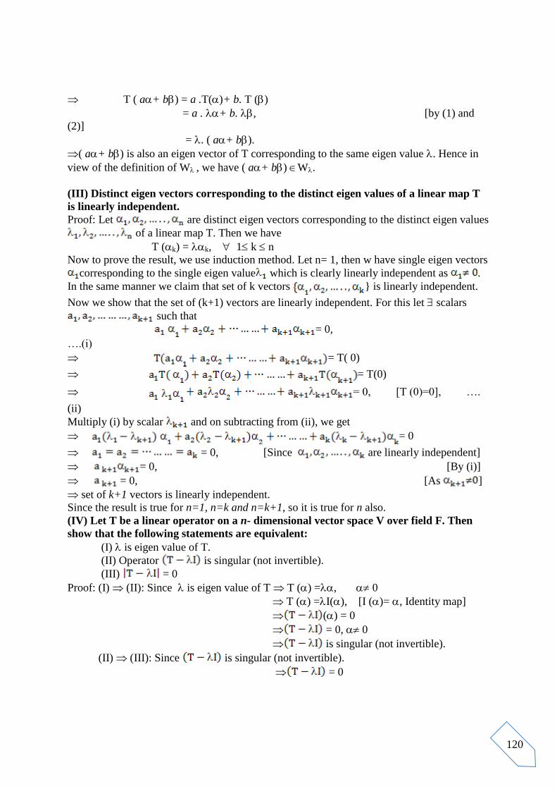
120
T ( a+ b) = a .T()+ b. T ()
= a . + b. , [by (1) and
(2)]
= . ( a+ b).
( a+ b) is also an eigen vector of T corresponding to the same eigen value . Hence in
view of the definition of W , we have ( a+ b) W.
(III) Distinct eigen vectors corresponding to the distinct eigen values of a linear map T
is linearly independent.
Proof: Let are distinct eigen vectors corresponding to the distinct eigen values
of a linear map T. Then we have
T (k) = k, 1 k n
Now to prove the result, we use induction method. Let n= 1, then w have single eigen vectors
corresponding to the single eigen value which is clearly linearly independent as .
In the same manner we claim that set of k vectors } is linearly independent.
Now we show that the set of (k+1) vectors are linearly independent. For this let scalars
such that
= 0,
….(i)
= T( 0)
= T(0)
= 0, [T (0)=0], ….
(ii)
Multiply (i) by scalar and on subtracting from (ii), we get
= 0
= 0, [Since are linearly independent]
= 0, [By (i)]
= 0, [As ]
set of k+1 vectors is linearly independent.
Since the result is true for n=1, n=k and n=k+1, so it is true for n also.
(IV) Let T be a linear operator on a n- dimensional vector space V over field F. Then
show that the following statements are equivalent:
(I) is eigen value of T.
(II) Operator is singular (not invertible).
(III) = 0
Proof: (I) (II): Since is eigen value of T T () =, 0
T () =I(), [I ()= , Identity map]
() = 0
= 0, 0
is singular (not invertible).
(II) (III): Since is singular (not invertible).
= 0

121
= 0.
(III) (I): Since = 0 = 0
() = 0, 0
T () =I()
T () =,[I ()= , Identity map]
is eigen value of T.
Solved Example on Eigen values, Eigen vectors of a matrix:
Example 1 Find the eigen values and eigen vectors of the matrix A= .
Solution: Eigen matrix of the given matrix A is
= =
Eigen equation is
=0 = 0
2 7 + 6 = 0
On solving we get = 1, 6.
Now let X= be the corresponding vector for = 1, then we have,
= 0
= 0
[Here rank of the matrix is 1, therefore Number of independent variable is 1.]
3x‟ +2x‟‟ =0,
x‟ = 2 if x‟‟= 3
Corresponding vector to = 1 is X= .
Similarly for = 6, corresponding vector is say X‟= , then
= 0
= 0
[Here rank of the matrix is 1, therefore Number of independent variable is 1.]
y‟ + y‟‟ =0,
y‟ = 1 if y‟‟= 1
Corresponding vector to = 6 is X‟= .
4.6.4 Diagonalization of linear transformation: Let T be a linear operator on a finite
dimensional vector space V. Then T is called diagonalizable if each vector of an ordered
basis
for V is an eigen vector of T. In other words T is diagonalizable if eigen vectors of T spans V.

122
4.6.5 Diagonalization of a Matrix: Let A= [aij ]n x n be a matrix of order n over a field F.
Then it
is said to be diagonalizable, if it is similar to a diagonal matrix over F. Thus to show that the
matrix A is diagonalizable, we find an invertible matrix P such that
P-1
AP = D.
Where D is diagonal matrix whose diagonal elements are the eigen values of matrix A.
WORKING RULE: To diagonalize the matrix A= [aij ]3 x 3 of order 3.
Step I: Find the eigen values i.e. (say).
Step II: Find corresponding vectors X 1, X2 and X3 to each ‟s.
Step III: Obtain invertible matrix P = [X 1, X2 , X3], by putting the values of vectors.
Step IV: Find P-1
[By any method].
Step V: Show P-1
AP = D, where D= Diag. [ ].
Solved Example on Diagonalization of a matrix:
Example 1 Show that the matrix A = is diagonalizable.
Solution: From page no. 29, corresponding vector to = 1 is X= and corresponding
vector to = 6 is X‟= . Therefore invertible matrix
P = [X, X‟] =
Now,
P-1
= = ,
Lastly
P-1
AP = . .
= =
= = Diag [1, 6 ]
Since P-1
AP = Diag [1, 6 ], hence matrix A is diagonalizable.
Example 2 Show that the matrix A = is diagonalizable
Solution: The eigen equation of matrix A is
=0
= 0
. ( 1). (2) = 0
= 0, = 1. =2

123
Let the corresponding eigen vector is X1 = [x1, x2, x3]‟ to eigen value = 0, then we have
on solving we get X1 = [4, -1, 0]‟. Similarly the corresponding eigen vector to eigen value
= 1 and = 2 is [4, 0, -1]‟ and [2, -1, 0]‟ respectively.
Therefore the invertible matrix is P = [X1, X2, X3]
P =
And so
P 1
= .
Thus
P-1
AP = = Diag [0, 1, 2].
CHECK YOUR PROGRESS:
Q. 1 Find matrix P, which will diagonalize the matrix A.
(i) A= (ii) A =
Ans. (i) P = , P-1
AP = Diag [0, 1, 2].
(ii) P= , P-1
AP = Diag[0, 3, 15]
Q. 2 Show that the following matrices are not diagonalizable:
(i) A = ( ii) A = (iii) A =
4.7 Bilinear, Quadratic and Hermitian Forms:
4.7.1 Bilinear Forms: A polynomial of sets of variables ( ) and
is called bilinear form and denoted by B(x, y). Symbolically we write
B (x, y) =

124
Here F and in each term the power of variables x and y is one-one and same. Also the
sum of powers of variables in each term is two .
REMARK: If and m= n, then bilinear form becomes quadratic form.
Example: Find the matrix B for the bilinear form B(x, y), where
B(x, y)=
Solution: We are given that
B(x, y)=
= +
Matrix form of the above expression is
B(x, y)= = X‟BY
Where X= , B= , Y=
4.7.2 Quadratic Forms: A polynomial of the form
q (x, x) = ,
Where F and in each term the total power of variables is two, is called quadratic form.
For example, q (x, x) = x12 + x1x2 + x2
2 and q(x, y) = x
2 + 5xy + y
2 etc.
WORKING RULE:
To obtain corresponding matrix of the quadratic given in terms of variables x, y, z. (say)
Step I: Write all the terms of x with x, y, z first i.e. x. x, x .y , x. z .
Step II: Then write all the terms of y with x, y, z i.e. y. x, y .y , y .z.
Step III: Lastly write all the terms of z with x, y, z i.e. z .x, z. y , z. z
Step IV: Write quadratic form in matrix equation form q= X‟ A X, A is coefficient
matrix and X is column vector of unknowns x, y ,z.
REMARK: (1) Since the terms containing x. y and y. x represent the same term, break such
terms into two equal parts. For example a term is say, 5xy. Then it can break into equal parts
viz.
5xy = x.y + y.x
Similarly, 2 y z = y z + z y etc.
(2) Matrix corresponding to a quadratic form is always a symmetric matrix.
Example 1: Find the symmetric matrix A for the quadratic form q, where
(i) q = x22y
23z
2 +4xy + 6xz 8yz
(ii) q = x12 + 4 x1x2 + 8 x2x3 + 10x3x1 12 x3
2.
Solution: (i) The given quadratic form q can be written as
q = xx + 2xy+ 3xz+2yx -2yy 4yz+ 3zx 4zy 3zz
[x y z]

125
q= X‟ A X, where X= , A =
Solution: (ii) The given quadratic form q = x12 + 4 x1x2 + 8 x2x3 + 10x3x1 12 x3
2 can be
written as
= x1x1 + 2 x1x2 + 5x1x3+2 x2 x1+0 x2 x2+4 x2x3 + 5x3x1 +4 x3x2 12 x3x3
= [x1 x2 x3]
q= X‟ A X, where X= , A =
Example 2: Find the quadratic forms corresponding to the matrix A= .
Solution: Let the required form is q = X‟AX, where X= , then
q = [x y z]
After matrix multiplications, we get
q = X‟AX = x2+z
2 +4xy + 6xz + 6yz.
4.7.3 Hermitian Form: An expression
h ( ) = X*HX = ,
is called Hermitian forms, where X=[ ]‟ Cn (unitary space) and H=[ ] n x m
be a hermitian matrix.
NOTE: (1) A matrix H is called Hermitian if H* = H. For example H= is
Hermitian.
(2) Hermitian forms h(x, y) = [x , y]
Example 1: Show that the following expression is a Hermitian form. Also obtain its
corresponding matrix:
x1x1 + x2x2 + (1+i) x1 x2 + (1i) x2 x1 +2 i x2 x3 2 i x3 x2 +4 x3 x1 + 4x1x3.
Solution: The given expression may be written as
h =x1x1 + (1+i) x1 x2 + 4x1x3+ (1i) x2 x1 + x2x2 +2 i x2 x3+4 x3 x1 2 i x3 x2 +0x3
x3
= ]
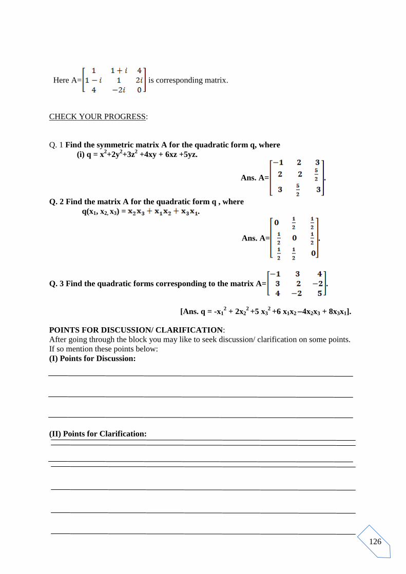
126
Here A= is corresponding matrix.
CHECK YOUR PROGRESS:
Q. 1 Find the symmetric matrix A for the quadratic form q, where
(i) q = x2+2y
2+3z
2 +4xy + 6xz +5yz.
Ans. A= .
Q. 2 Find the matrix A for the quadratic form q , where
q(x1, x2, x3) = .
Ans. A= .
Q. 3 Find the quadratic forms corresponding to the matrix A= .
[Ans. q = -x12 + 2x2
2 +5 x3
2 +6 x1x2 4x2x3 + 8x3x1].
POINTS FOR DISCUSSION/ CLARIFICATION:
After going through the block you may like to seek discussion/ clarification on some points.
If so mention these points below:
(I) Points for Discussion:
(II) Points for Clarification:

127
REFERENCES:
1. Linear Algebra, Kenneth Hoffman and Ray Kunz, Prentice-Hall Inc.
2. Algebra, M. Artin, Prentice-Hall of India Pvt. Ltd., New Delhi
3. Introduction to Modern Algebra, Neal H. Macoy, Bostan, Allay & Bacon, Inc.
4. Linear Algebra: Ideas and Application, Richard C. Penney, Wiley Inter-Science, A
John Wiley and Sons. Inc. Publication
B. Sc. III
LINEAR ALGEBRA BLOCK III : UNIT V- INNER PRODUCT SPACE
DR. SANJAY JAIN GOVT. HOLKAR SCIENCE COLLEGE, INDORE

128
BLOCK- III
LINEAR ALGEBRA
Our main object is to study vector spaces in which it makes sense to tell
the length of a vector and angle between two vectors. We shall do this by
studying a special type of scalar valued function namely inner product space on
the pair of vectors
This unit presents the basic concepts of inner product spaces along with
their elementary properties. This product also introduces the well known
geometrical notions of length of vectors and the angle between them. Further
we shall discuss the concept of orthogonality and the solutions of the problems
of the Existence of the orthonormal basis in a finite dimensional inner product
space through Gram-Schmidt process.
In the end of this unit the Bessel‟s inequality for finite dimensional vector
spaces has also been discussed. A set of unsolved problems as an exercise has
been given to the readers.
Object: At the end of this block a reader would be able to apply the ideas in
solving the related problems.
UNIT – V
INNER PRODUCT SPACES
Structure:
5.1 Brief Review
5.2 Definition and examples of Inner Product spaces
5.3 Properties of Inner Product Space
5.4 Orthogonal and Ortho-normal Set and Bases
5.5 Gram- Schmidt Orthogonalization Process
5.6 Bessel’s Inequality for Finite Dimensional Spaces
*Points for Discussion/ Clarification
BLOCK INTRODUCTION

129
**References
5.1 Brief Review:
5.1.1 A complex number Z = having real and imaginary part. Here x is called real part
and y is called imaginary part.
NOTE: (1) Coefficient of i always known as imaginary part in a complex number. If y =0
then number z = becomes real.
(2) Real part of a complex number z = is written as Re Z, while imaginary part as Im
Z.
5.1.2 Some Properties of Complex number:
(I) Conjugate of a complex number Z = is obtained by changing the sign of its
imaginary part with the complementary signs i.e. + with , or with + .
(II) Z + Z = ( ) + ( ) = 2x = 2 Re Z
(III) Z Z = ( ) ( ) = 2y = 2i Im Z
(IV) Z. Z = ( ). ( ) = x2 +y
2 = Z
2.
Here Z means modules or absolute value or magnitude of Z and defined Z= ( x2+y
2).
(V) Z= 0 if and only if x=0 , y=0
(VI) Z= Z
(VII) (Z) = Z
(VIII) Z1+ Z2 Z1+Z2
(IX) (Z1+ Z2 ) Z1+ Z2
(X) (Z1. Z2 ) = Z1.Z2 , where Z1 andZ2 are two complex numbers.
5.1.3 Row and Column vectors:
A matrix containing a single row is called Row- vector while a matrix
containing a single column is known as Column- vector. For example
X = is a row-vector and Y = is a column-vector .
5.1.4 Transpose and Tranjugate of a matrix:
Transpose of a matrix is obtained by inter-changing rows into columns while
tranjugate of a matrix is obtained by taking whole conjugate of transpose matrix.
Things to Remember: Tranjugate = Transpose + Conjugate
For example: If A= , then its transpose is A‟ =
And its tranjugate is =
5.1.5 Inner Product Space:
Let X=( ) and Y = ( ) are two row vectors. Then the
inner product of X and Y symbolically denoted by (X, Y) is defined as:
(X, Y) = X = X (Y)’ =
….(1)

130
Things to Remember: If vector Y is real then (1) becomes
(X, Y) = X =
For example: (1) Let X = and Y = , then the inner product of X and
Y is
(X, Y) = X = 1.3 + 2.4 +3.5 = 3 + 8 + 15 = 26 [since Y is real]
(2) If X= and Y = , then the inner product of X and Y is
(X, Y) = X = X (Y)’
=
= 1.( )+ ( )= 114i .
5.2 Definition and Examples of Inner Product Space:
5.2.1 Definition: Let V (F) be a vector space and F is field of real or complex numbers.
Inner
product V V F is defined on V. Then V (F) is called Inner product space, if the
following properties are satisfied:
(1) Non-negativity: α V, ( α, α) 0 and ( α, α)= 0 α = 0
(2)Conjugate Symmetry: (α, β)= ( β, α) , α, β V
(3) Linearity: (a α + b β , ) = a (α, ) + b (β, ), α, β, V and a, b F
Things to Remember:
(1) If F= R , then conjugate symmetry property known as symmetric property because
in this case inner product (α, β)= real quantity.
(2) Length of a vector α in inner product space is denoted by and defined as
= ( α, α)
For example: If α= (2, 3), then length of is = ( α, α),
Now ( α, α)= 2.2 + 3.3 = 13, therefore = 13.
(3) Unit Vector: Let V (F) is an inner product space and α V (F). Then vector α is
called of unit length if = 1.
For example: If α= (0, 1), then length of is = 1, therefore α is a unit vector.
( 4) To prove that any vector space V is an inner product space , we simply show that all
three properties of 5.2.1 satisfied in V.
5.2.2 Examples based on Inner Product Space:
Example 1 Show that V2 (R) is an inner product space w.r.t. the inner product
( , ) = ( ) , , V2 (R). …….(1)
Solution: Let = ( ), = ( ) V2 (R) are two arbitrary elements of V2 (R).
To prove that vector space V2 (R) is an inner product space , we simply show that all three
properties of 5.2.1 satisfied in V2 (R).
(I) Non-negativity:
α V, ( α, α) = [ by (1) ]
= 0 [square of any number is always positive.]
Also,

131
(α, α)
[sum of two positive number is zero, then both number must be zero.]
= 0
(II) Conjugate Symmetry: we have
( , ) = ( ) , , V2 (R)
Also ( , ) = ( ) = ( ),
On taking conjugate both side, we get
( , ) =( )= ( )= ( , ), [ since F = R
here]
(III) Linearity: Let = ( ), = ( ),= ( ) V2 (R) are three arbitrary
elements of V2 (R) and a, b R, then
(a α + b β) = a ( ) + b ( )
= ( ) + ( ) = ( + )
Therefore
(a α + b β , ) = 3( ) +2 ( + )
On solving, we get
= ( ) + ( )
= ( ) +b ( )
= a (α, ) + b (β, ),
Therefore, (a α + b β, ) = a (α, ) + b (β, ), Since all the properties of inner product satisfied in V2 (R) , hence V2 (R) is an inner product
space.
Example 2 Examine that V2 (R) is an inner product space w.r.t. the following inner
product
(i) ( , ) = , =( ), =( ) V2 (R).
(ii)( , ) = , =( ), =( ) V2 (R).
Solution: (i) α V, (α, α) =
= = 0, If
Here (α, α) 0. Clearly non-negativity property not holds true, hence V2 (R) is not an inner
product space.
Solution (ii): (1) Non-negativity: By the definition
( , ) =
=
= ( )2 + 0, [square of any number is always positive.]
(2) Conjugate Symmetry:
( , ) = , =( ), =( ) V2 (R).
=

132
= ( ), [In R, = ]
= ( , ) .
(3) Linearity: Let = ( ), = ( ),= ( ) V2 (R) are three arbitrary elements
of
V2 (R) and a, b R, then
(a α + b β) = a ( ) + b ( )
= ( + )
Therefore
(a.α + b β,) = ( ) ( + ) ( ) +2( +
)
On solving and then collecting the terms of a and b, we get
= ) +
= a (α, ) + b (β, ),
Therefore, (a α + b β, ) = a (α, ) + b (β, ), Hence in view of (1), (2) and (3),V2 (R) is an inner product space.
CHECK YOUR PROGRESS:
Q.1Which of the following in V2(R) defines an inner product space, where = ( ),
= ( )
(i) ( , ) =
(ii) )( , ) =2
(iii) ( , ) =
Q.2 Show that (, ) = , =( ), =( ) V2 (R) do not define
an inner product space in V2 (R).
5.3 Some Properties of Inner Product Space:
(I) 0 and = 0 = 0.
Proof: By the definition of inner product space,
α V, ( α, α) 0 and ( α, α)= 0 α = 0
= .
Proof: By the definition of norm or length of a vector , we have
= (
= ( ] [since Z = Z]
= ( ] = ( = . [since Z.Z = ]
Schwartz’s Inequality: In an inner product space V (F),
Proof: Case I Let = 0 , then = 0 and so we have = 0 ……..
(i)
(, ) = (0, ) = (0.0, ) =0 . (0, ) = 0 = 0 ……..
(ii)
Therefore in view of (i) and (ii), we have
=
Case II Let 0 , then 0, and so 0.
Now we can consider a vector = ,
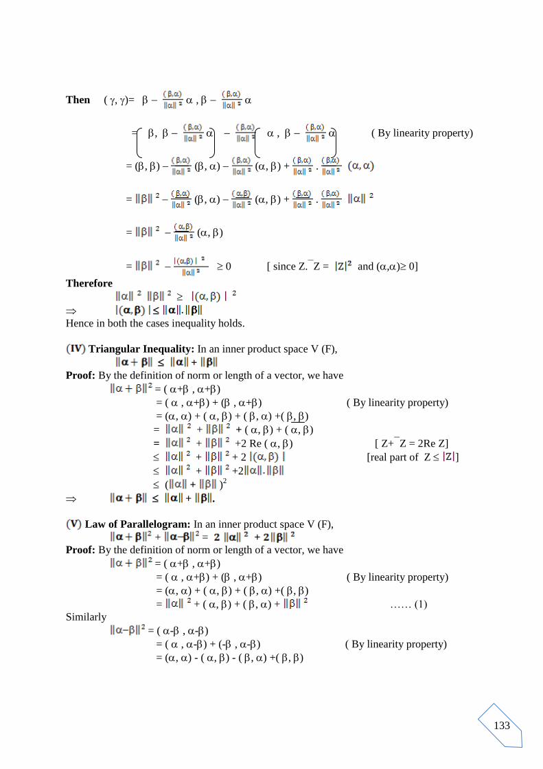
133
Then ( , )= ,
= , , ( By linearity property)
= (, ) (, ) (, ) + .
= (, ) (, ) + .
= (, )
= 0 [ since Z.Z = and (,) 0]
Therefore
Hence in both the cases inequality holds.
Triangular Inequality: In an inner product space V (F),
+
Proof: By the definition of norm or length of a vector, we have
= ( + , +)
= ( , +) + ( , +) ( By linearity property)
= (, ) + ( , ) + ( , ) +( , )
= + + ( , ) + ( , )
= + +2 Re ( , ) [ Z+Z = 2Re Z]
+ + 2 [real part of Z ]
+ +2
( + )2
+ .
Law of Parallelogram: In an inner product space V (F),
+ = +
Proof: By the definition of norm or length of a vector, we have
= ( + , +)
= ( , +) + ( , +) ( By linearity property)
= (, ) + ( , ) + ( , ) +( , )
= + ( , ) + ( , ) + …… (1)
Similarly
= ( - , -)
= ( , -) + (- , -) ( By linearity property)
= (, ) - ( , ) - ( , ) +( , )

134
= + ( , ) - ( , ) + …… (2)
On adding (1) and (2), we get the required result i.e.
+ = + .
THINGS TO REMEMBER: Two vectors and are said to be linearly dependent if they are
scalar multiple to each other. Means a F such that = a. or = a.. For example if
= (1, 1) and = (3, 3) are two vectors , then clearly they are linearly dependent as = 3. .
(VI) In an inner product space V (F), two vectors and are linearly dependent if and
only if =
Proof: Part I : Let Two vectors and are linearly dependent, then a F such that =
a..
We shall prove that = .
Now = = . …… (i)
Again = = . = . …….(ii)
So by (i) and (ii), we have
= .
Part II : Let = .
We shall prove that vectors and are linearly dependent. For this we shall prove that can
be express as scalar multiple of .
Case 1: Let one of the vector is zero, say = 0.
Then the result is obviously true as we know that set of vectors containing a zero vector is
always linearly dependent.
Case 2: If 0, then 0
Now we have, =
= = [since ]
= , where = , = 1 being unit vector. ….. (iii)
Again we consider 2 = ( )
= { }
= 2 { }
= { [By (iii)]
= 0
2 = 0 then = 0
[By (iii)]
( )
a. , where a= ( ) is a scalar quantity.
Vectors and are linearly dependent.

135
(VII) In an inner product space V (F), = + , then the vectors and
are linearly dependent but converse is not true necessarily.
Proof: Given: = +
Squaring both sides, we get
= + + 2 . …….. (1)
Also we know that,
= ( )
= (, ) + (, ) + (, ) + (, )
= + ( , ) + ( , ) +
= + +2 Re ( , ) [ Z+Z = 2Re Z] ……...(2)
From (1) and (2) we get
. = Re ( , ) ……..
(3)
Also we know that
Re ( , ) ……...
(4)
Therefore by (3) and (4) we get
. ……..
(5)
But by Schwartz‟s inequality, we have
……..
(6)
In virtue of (5) and (6), we have
=
Vectors and are linearly dependent. ( By property VI).
Converse Part: we shall prove this part with an example. Let = (1, 1) , = (2, 2) V2
(R), then clearly = 2 and hence they are linearly dependent. We shall now show that
+ .
Here + = (1, 1) + (2, 2) = (1, 1),
Therefore
= ( )
= 1.1 + (1).(1) = 2
= 2 . ……. (7)
Also
= (, ) = 1.1 + (1).(1) = 2 = 2
And
= ( , ) = 2.2 + (2).(2) = 8 = 8
Therefore
+ = 2 +8 = 32 ……..
(8)
From (7) and (8), we have
+ .

136
Converse part not true necessarily.
(VIII) Distance between two Vectors in an Inner Product Space: Let V (F) is an inner
product space and let and are two vectors. Then distance between two vectors and is
denoted by d (, ) and defined as
d (, ) = = ( )
For example let = (1, 1) , = (2, 2) V2 (R), then = (1, 1) (2, 2) = (3, 3) and
therefore
d (, ) = = ( )
= ( = 18= 32.
Therefore distance between two vectors and is 32.
CHECK YOUR PROGRESS:
Q.1 If and are vectors in an inner product space V (F) and a, b F, then show that the
following equalities hold:
( i) = 2
2 + a.b (, ) +a.b (, ) +
2
2+
(ii) Re (, ) =
(iii) 4 (, ) = + i i
(iv) (, ) = Re (, ) + i Re (, i).
Q.2 Let V (F) be a vector space of polynomials in x. Let the inner product in V (F) is
defined as: ( p, q) = ,Where p= p(x) and q =q(x) V. Then if p(x) = x +
2, q(x)= 2x3 , find
(i) ( p, q) (ii) (iii) (iv) angle between p and q .
Hint: We have p(x) = x + 2 and q(x) = 2x3, therefore
= (x + 2).( 2x3) = 7x 6
Therefore ( p, q) = = = = = ( ).
Similarly the value of = ( p, p) and = ( q, q) are left to the reader as exercise.
Now let be the angle between p and q , then we have

137
= =
On solving, we get = .
5.4 Orthogonal and Ortho-normal Set and Bases:
5.4.1 Definition of Orthogonal Vectors: Let and are vectors in an inner product space V
(F)
Then and are said to be orthogonal if ( , ) = 0 and written as .
In brief ( , ) = 0.
For example: Let = (1, 0, 1) and = (1, 0, 1) are two vectors in an inner product space V3
(F). Then , as the inner product of and be zero i.e.
( , ) = 1.1 + 0.0 + 1.(1) = 0
5.4.2 Definition of Orthogonal Vectors to a set: Let V (F) be an inner product space, and
V Then is said to be orthogonal to subset S of V (F), if it is orthogonal to each element
of S. In brief
S , S
5.4.3 Definition of Orthogonal set: Let V (F) is an inner product space, and S V (F), then
S is called orthogonal if any two elements of S are orthogonal to each other. In brief ,
V (F) and , we have i.e. ( , ) = 0.
5.4.4 Definition of Orthogonal sets: Let V (F) is an inner product space, S and T V (F).
Then S and T are called orthogonal to each other if every element of S is orthogonal to each
element of T.
In brief, S T , S and T
5.4.5 Definition of Orthonormal set: Let V (F) is an inner product space, and S V (F).
Then S is called orthonormal set, if
THINGS TO REMEMBER: (1) To show that the given set of vectors are orthonormal‟ we
simply show that the inner product of the same element is 1 and inner product of different
vectors is 0 i.e.

138
( ) =
(2) If be the angle between and , then we have = . If , then =
And so
= 0 =
5.4.6 Solved Problems on Orthogonal and Ortho-normal Vectors:
Example 1 Let V (F) is an inner product space and let , V (F) such that ,
= = 1. Then show that the distance between and i.e. d ( , ) = 2 .
Solution: Given: and = = 1.
Now by the definition of distance between two vectors, we have
d ( , ) =
= ( )
= [(, ) + (, ) + (, ) + (, )]
= ( , ) ( , ) + }
= (1 0 0 + 1) = 2. [as (, ) = 0 and = =
1]
d ( , ) = 2.
Example 2 Let V (R) is an inner product space and let , V (F). If = , then
show that ( + ) and ( ) are orthogonal.
Solution: To show that ( + ) and ( ) are orthogonal, we shall show that the inner
product of these two is zero i.e. ( + , ) = 0.
Now ( + , ) = (, ) + (, ) + (, ) + (, )
= ( , ) + ( , )
= ( , ) + (, ) [If F = R, then Z= Z]
= 0 [Since = ]
( + ) ( ).
Example 3 Show that an orthogonal set of non zero vectors in an inner product space V
(F) is linearly independent.
Solution: Let S = { , …………… , } be an orthogonal set of non zero vectors in an
inner product space V (F). Since S is orthogonal, by the definition of orthogonal set,
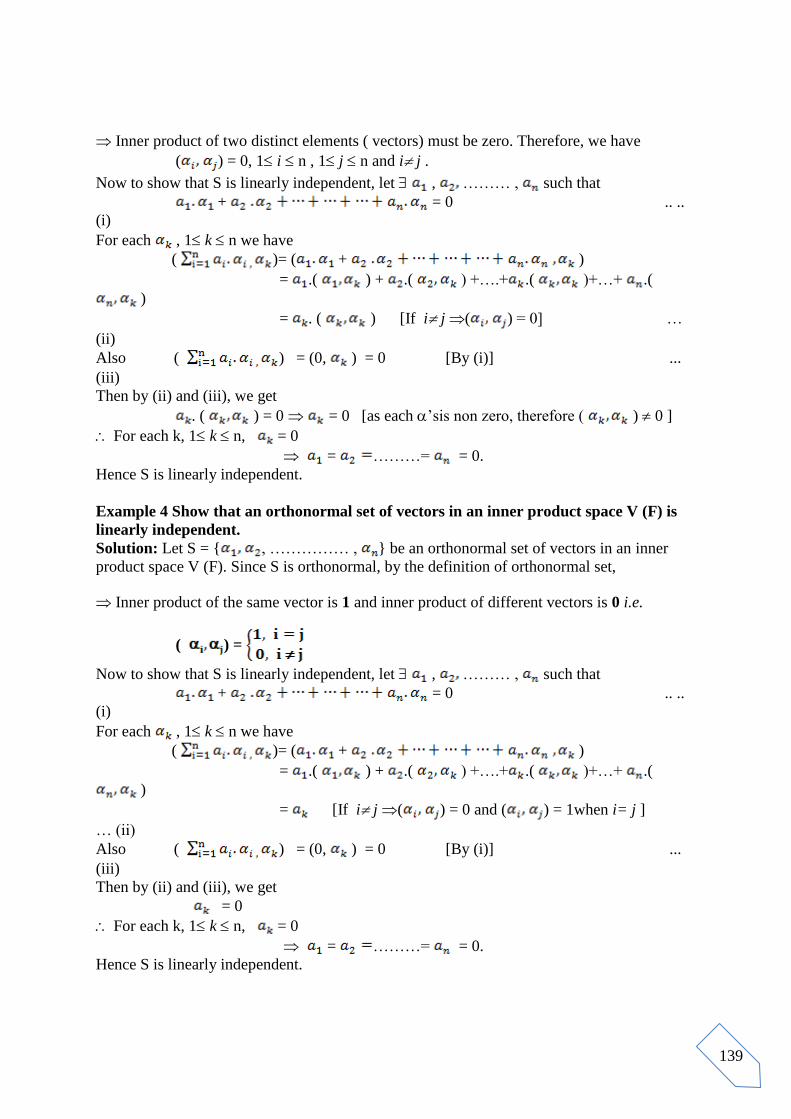
139
Inner product of two distinct elements ( vectors) must be zero. Therefore, we have
( ) = 0, 1 i n , 1 j n and i j .
Now to show that S is linearly independent, let , ……… , such that
+ = 0 .. ..
(i)
For each , 1 k n we have
( )= ( + )
= .( ) + .( ) +….+ .( )+…+ .(
)
= . ( ) [If i j ( ) = 0] …
(ii)
Also ( ) = (0, ) = 0 [By (i)] ...
(iii)
Then by (ii) and (iii), we get
. ( ) = 0 = 0 [as each ‟sis non zero, therefore ( ) 0 ]
For each k, 1 k n, = 0
= ………= = 0.
Hence S is linearly independent.
Example 4 Show that an orthonormal set of vectors in an inner product space V (F) is
linearly independent.
Solution: Let S = { , …………… , } be an orthonormal set of vectors in an inner
product space V (F). Since S is orthonormal, by the definition of orthonormal set,
Inner product of the same vector is 1 and inner product of different vectors is 0 i.e.
( ) =
Now to show that S is linearly independent, let , ……… , such that
+ = 0 .. ..
(i)
For each , 1 k n we have
( )= ( + )
= .( ) + .( ) +….+ .( )+…+ .(
)
= [If i j ( ) = 0 and ( ) = 1when i= j ]
… (ii)
Also ( ) = (0, ) = 0 [By (i)] ...
(iii)
Then by (ii) and (iii), we get
= 0
For each k, 1 k n, = 0
= ………= = 0.
Hence S is linearly independent.

140
THINGS TO REMEMBER:
(1) L (S) means linear span of set S i.e.set of all possible linear combinations of elements
of S.
(2) S can be express as a linear combination of elements of S.
Example 5 Let V (F) is an inner product space and let S = { , …………… , } be an
orthogonal set of non zero vectors in V. If V is in the linear span of S i.e. L (S) , then
show that
=
Solution: Since S = { , …………, } is orthogonal, by the definition of orthogonal
set,
Inner product of two distinct elements (vectors) must be zero. Therefore, we have
( ) = 0, 1 i n , 1 j n and i j .
Also L (S) can be express as a linear combination of elements of S. Let
, ……… , F such that
= + , …..
(i)
For each , 1 k n we have
( , ) =( )
= ( + )
= .( ) + .( ) +….+ .( )+…+ .( )
= . ( ) [If i j ( ) = 0]
= .
= , [for 1 k n] …
(ii)
On putting the values of , ……… , from (ii) to (i), we get
= .
5.4.6 Orthogonal Basis: Let V (F) is an inner product space and let S = { , …… , }
be
an orthogonal set in V. If S forms a basis of V (F), then S is called orthogonal basis.
5.4.6 Orthonormal Basis: Let V (F) is an inner product space and let S = { , ……
, } be
an orthonormal set in V. If S forms a basis of V (F), then S is called orthonormal basis.
5.4.7 Normalize Vector of a Vector : Let V (F) is an inner product space and let V.
Then
Normalize vector of is .
For example: Let = (1, 2, 3) V3, then by the definition of norm we have,
= (, ) = [ 1.1 + 2.2 + 3.3] = 14
Then Normalize vector of is
= (1, 2, 3) or ( ).

141
5.5 Gram- Schmidt Orthogonalization Process:
This process is used to find an orthonormal basis for a finite dimensional inner product space.
As per the Gram- Schmidt Orthogonalization theorem we say that every finite dimensional
inner
product space has a orthonormal basis. Proof of this theorem is easily understand with the
help of
the steps given below. Therefore proof of this theorem is left to the reader as an exercise.
5.5.1: Working rule of Gram- Schmidt Orthogonalization Process to numericals:
Given: Basis set S = { , …… , }of a n- dimensional inner product space V (F). Then,
Part I: To obtained Orthogonal Basis: Assume that S‟= { , …, }is Orthogonal Basis,
then
Step I: Take =
Step II: To find , use relation =
Step III: To find , use relation =
Step IV: The above procedure will continue till the value of last element of assumed
Orthogonal Basis not obtained. To find , we have
= …….
Finally we got the actual Orthogonal Basis.
Part II: To obtained Orthonormal Basis: Assume that S‟‟= { , …, }is Orthonormal
Basis.
Then normalize each element of orthogonal basis S‟ i.e. , , ……….. , .
Lastly assumed that , = , ……… , = to get the required
Orthonormal Basis.
5.5.2Solved Examples related to Gram- Schmidt Orthogonalization Process:
Example 1 Obtain orthonormal basis of the given basis { } for V3 (R) by using
Gram-
Schmidt process, where = (1, 1, 1).
Solution: First we assume that = =
Now to find , we have
=
= [since = ( )
=1.1+0.0+0.0]
= (
=

142
Again to find , we have
=
= (1, 1, 1) ,
= (1, 1, 1)
=
Therefore Orthogonal Basis is { = = = }.
To obtained Orthonormal Basis we assume that { , } is Orthonormal Basis, where
= ,
= = = ,
And
= = ,
Therefore required Orthonormal Basis is { = = }.
Example 2 Obtain orthonormal basis of the given basis { } for V3 (R) with
standard
inner product using Gram-Schmidt process, where = (1, 2, 1).
Solution: First we assume that = =
Now to find , we have
=
=
[since = ( ) =1.1+1.1+1.1]
= (
=
Again to find , we have
=
= (1, 2, 1) ,
= (1, 2, 1)
=
Therefore Orthogonal Basis is { = = = }.
To obtained Orthonormal Basis we assume that { , } is Orthonormal Basis, where
= ,
= = = ,
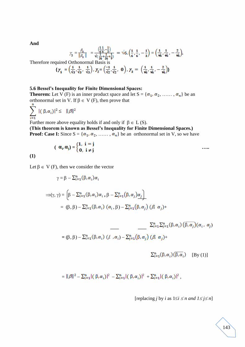
143
And
= = = .
Therefore required Orthonormal Basis is
{ = = }
5.6 Bessel’s Inequality for Finite Dimensional Spaces:
Theorem: Let V (F) is an inner product space and let S = { , …… , } be an
orthonormal set in V. If V (F), then prove that
Further more above equality holds if and only if L (S).
(This theorem is known as Bessel’s Inequality for Finite Dimensional Spaces.)
Proof: Case I: Since S = { , …… , } be an orthonormal set in V, so we have
( ) = …..
(1)
Let V (F), then we consider the vector
=
(, ) = ,
= (, ) , ) +
)
= (, ) ) +
[By (1)]
= 2
2 +
2 ,
[replacing j by i as 1i n and 1 j n]

144
= 2
…..
(2)
Now we know that
(, ) 0 2 0
2
Case II: Let the equality holds 2 = ,
Then, we have 2 = 0 ,
(, ) = 0, then = 0
= 0
=
is the linear combination of , …… , .
L (S).
Converse part: Let L (S),
can be express as a linear combination of , …… , .
So let = , then we have
= 0
(, ) = 0, then = 0
Then, we have 2 = 0 , [by (2)]
2 = ,
hence equality holds if and only if L (S).
CHECK YOUR PROGRESS:
Find the orthonormal basis using Gram-Schmidt process for V3 (R) with the standard
inner product relative to the basis given below:
Q.1 = (2, 1, 1).
[Ans. { = = }]
Q.2 = (0, 3, 4)
[Ans. { = = }]
Q.3 = (1, 2, 3)
[Ans. { = = }]
POINTS FOR DISCUSSION/ CLARIFICATION:
After going through the block you may like to seek discussion/ clarification on some points.
If so mention these points below:
(I) Points for Discussion:

145
(II) Points for Clarification:
REFERENCES:
1. Topics in Algebra, I.N.Herstien
2. Linear Algebra, Kenneth Hoffman and Ray Kunz, Prentice Hall Inc.
3. Algebra M. Artin, Prentice Hall of India Pvt. Ltd., New Delhi.