absorfrion heat pump for space applications final report …

ABSORFrION HEAT PUMP FOR SPACE APPLICATIONS

FINAL REPORT

NASA Grant # NAG 9-613

December, 1993

Lamar University

College of EngineeringBeaumont, Texas

Tuan Nguyen, Ph.D., P.E., Principal InvestigatorWilliam E. Simon, Ph.D., P.E., Research Associate

Gopinath R. Warrier, M.S., Graduate AssistantWoranun Woramontri, M.S., Graduate Assistant

•ABSTRACT

Absorption Heat Pumps for Space Applications

In the first part of this study, the performance ofthe Absorption Heat Pump (AFIP)

with water-sulfuric acid and water-magnesium chloride as two new refrigerant-absorbent

fluid pairs was investigated. A model was proposed for the analysis of the new working

pairs in a heat pump system, subject to different temperature lifts. Computer codes were

developed to calculate the Coefficient of Performance (COP) of the system with the

thermodynamic properties of the working fluids obtained from the literature. The study

shows the potential of water-sulfuric acid as a satisfactory replacement for water-lithium

bromide in the targeted temperature range. The performance of the AHP using water-

magnesium chloride as refrigerant-absorbent pair does not compare well with those

obtained using water-lithium bromide.

The second part of this study concentrated on the design and testing of a simple

ElectroHydrodynamic (EHD) Pump. A theoretical design model based on contitluum

electromechanics was analyzed to predict the performance characteristics of the

electrohydrodynamic (EHD) pump to circulate the fluid in the absorption heat pump. A

numerical method of solving the governing equations was established to predict the

velocity profile, pressure - flow rate relationship and efficiency of the pump. The

predicted operational characteristics of the EHD pump is comparable to that of

turbomachinery hardware; however, the overall efficiency of the electromagnetic pump is

much lower. An experimental investigation to verify the numerical results was conducted.

The pressure - flow rate performance characteristics and overall efficiency of the pump

obtained experimentally agree well with the theoretical model.

List of Tables

List of Figures

Section I

Introduction

TABLE OF CONTENTS

Page

.................................................. V

................................................ vii

..............................................

Conclusion

References

Section II

Introduction

Characteristics of Refrigerant-Absorbent Pairs ........................ 3

Desirable Properties of Refrigerant-Absorbent Pairs ................ 3

Thermodynamic Properties of Water-Sulfuric Acid Fluid Pair ......... 5

Thermodynamic Properties of Water-Magnesium Chloride FluidPair

..............................................

Absorption Heat Pump Analysis ................................. 9

Absorption Heat Pump Configuration .......................... 9

Governing Equations and Performance Calculation ............... 10

Results and Discussion ....................................... 14

Heat Pump Performance .................................. 14

AHP Performance with the Water-Sulfuric Acid Pair ......... 14

AHP Performance with the Water-Magnesium Chloride

Pair ........................................ 16

............................................... 7

.............................................. . 18

............................................... 4

Theoretical Modeling of an EHD Pump ........................... 46

iii

NumericalMethod.......................................... 50

Experimental Apparatus and Instrumentation ........................ 52

Experimental Procedure .................................. 54

Results and Discussion ....................................... 57

Numerical Results ...................................... 57

Numerical Results for the Velocity Profile ................ 57

Numerical Results for the Pressure-Flow Rate Performance

Characteristics ................................. 58

Numerical Results for Pump Efficiency .................. 59

Effects of Magnetic Flux Density and Voltage Across

the Electrodes on EHD Pump Efficiency .......... 59

Effect of Flow Rate of EHD Pump Efficiency ........ 61

Experimental Results ......................... . .......... 62

Experimental Results of Pressure-Flow Rate Relationship ...... 62

Experimental Results of Overall Efficiency ................. 63

Conclusion and Recommendations ............................... 65

References ............................................... 7

Appendix ............................................... 118

iv

Table

Section I

1.

LIST OF TABLES

Page

Total Pressure-Temperature-Concentration Correlation for Water-Sulfuric

Acid Solution .................................................................................................. 20

2. Relative Volatility Relationship for Water-Sulfuric Acid

Solution ........................................................................................................... 22

3. Enthalpy-Temperature-Concentration Correlation for Water-Sulfuric

Acid Solution ................................................................................................... 25

4. Maximum Solubility of Magnesium Chloride as a Function of Solution

Temperature ................................................................................................... 26

5. Vapor Pressure of Water-Magnesium Chloride Solution

[303K _<T _<343K, 0.5 < m _<8.6] .................................................................. 29

6. Vapor Pressure of Water-Magnesium Chloride Solution

[320K < T 400K, 1.051 < m _<4.104] ............................................................ 30

7. Enthalpy of Water-Magnesium Chloride Solution

[25°C _<T < 80oc, 0.1 < m < 2.0] .................................................................. 31

8. Enthalpy of Water-Magnesium Chloride Solution

[373.15K _<T < 472.95K, 0.0 < m < 5.6] ........................................................ 32

9. Water-Sulfuric Acid System ................................................................................ 34

10. Water-Lithium Bromide System (I) ..................................................................... 35

11. Water-Magnesium Chloride System .................................................................... 39

12. Water-Lithium Bromide System (II) ................................................................... 40

Section II

1. Experimental Conditions for the Magnetic Flux Density and Voltage

Across the Electrodes ...................................................................................... 73

.

.

Magnetic Flux Density and Voltage Across the Electrodes for

Figures 17 to 28 ............... :.............................................................................. 92

Magnetic Flux Density and Voltage Across the Electrodes for

Figures 29 to 40 ............................................................................................. 105

Properties of Copper Sulfate Solution ............................................................... 131

Properties of Standard Annealed Copper Wire ................................................. .135

vi

LIST OF FIGURES

Figure Page

;Section I

1. Freezing Points of Water-Sulfuric Acid Solution at Various Concentrations ....... :..21

2. Relative Volatility of Water-Sulfuric Acid Solution at P = Pg ................................. 23

3. Relative Volatility of Water-Sulfuric Acid Solution at Various Pressures ............ _..24

4. Maximum Solubility of Magnesium Chloride in Solution ........................................ 27

5. Relative volatility of Water-Magnesium Chloride Solution at Various

Pressures ............................................................................................................ 28

6. Absorption Heat Pump Configuration .................................................................... 33

7. Cooling Mode COP Comparison [Water-Sulfuric Acid Vs.

Water-Lithium Bromide] .................................................................................... 36

8. Variation in Specific Circulation Rates with Temperature [Water-Sulfuric

Acid Vs. Water-Lithium Bromide] ...................................................................... 37

9. Heating Mode COP Comparison [Water-Sulfuric Acid Vs.

Water-Lithium Bromide] ................................................................................. :..3 $

10. Cooling Mode COP Comparison [Water-Magnesium Chloride Vs.


11. Variation in Specific Circulation Rates with Temperature [Water-

Magnesium Chloride Vs. Water-Lithium Bromide] ............................................ 42

12. Heating Mode COP Comparison [Water-Magnesium Chloride Vs.


Section II

1. Configuration of an EHD Pump .......................................................................... 68

2. Grid Point Layout used in the Finite Difference Method ...................................... 69

3. Experimental Apparatus ...................................................................................... 70

vii

.

5.

6.

7.

8.

9.

10.

11.

12.

13.

14.

15.

16.

17.

18.

19.

20.

21.

Pump Layout used in the Exl_eriments ................................................................ 71

Details of the Electromagnet ............................................................................... 72

An Example of the Velocity Profile Obtained Numerically ................................... 74

The Velocity Profile for V = 10 V (B = 0.2 T, P = 30 Pa) ................................... 75

The Velocity Profile for V = 15 V (B = 0.2 T, P = 30 Pa) ................................... 76

The Velocity Profile for V = 20 V (B = 0.2 T, P = 30 Pa) ................................ _..77

The Velocity Profile for B = 0.2 T (V = 15 V, P = 30 Pa) ................................... 78

The Velocity Profile for B = 0.3 T (V = 15 V, P = 30 Pa) .............. . .................... 79

The Velocity Profile for B = 0.4 T (V = 15 V, P = 30 Pa) ................................... 80

The Pressure - Flow Rate Relationship at Constant Voltage (V = 15 V) .............. 81

The Pressure - Flow Rate Relationship at Constant Magnetic Flux

Density ( B = 0.2 T) ........................................................................................ 82

Contour Plot of the Internal Efficiency at Constant Volumetric Flow Rate

(Q = 1 x 10 4 m3/s) .......................................................................................... 83

Contour Plot of the Electrical Efficiency at Constant Volumetric Flow Rate

(Q = 1 x 10 -4 m3/s) .......................................................................................... 84

Contour Plot of the Overall Efficiency at Constant Volumetric Flow Rate

(Q = 1 x 10 -4 m3/s) ........................................................................................... 85

Internal Efficiency as a Function of Applied Voltage at Constant MagneticFlux Density (B = 0.2 T) .................................................................................. 86

Internal Efficiency as a Function of Magnetic Flux Density at ConstantVoltage (V = 15 V) ......................................................................................... 87

Electrical Efficiency as a Function of Magnetic Flux Density at Constant

Voltage (V = 15 V) ......................................................................................... 88

Electrical Efficiency as a Function of Applied Voltage at Constant Magnetic

Flux Density (B = 0.2 T) ............................................................................. . .... 89

viii

22.

23.

24.

25.

26.

27.

28.

29.

30.

31

32.

33.

34.

35.

Overall Efficiency as a Function of Magnetic Flux Density at Constant

Voltage (V = 15 V) ......................................................................................... 90

Overall Efficiency as a Function of Applied Voltage at Constant Magnetic

Flux Density (B = 0.2 T) .................................................................................. 91

Pressure - Flow Rate Relationship Obtained Numerically and

Experimentally for V = 10 V and B = 0. I T ...................................................... 93


Experimentally for V -- 10 V and B = 0.2 T ..................................................... 94


Experimentally for V = 10 V and B = 0.3 T ..................................................... 95


Experimentally for V = 10 V and B = 0.4 T .................................................. :..96


Experimentally for V = 15 V and B = 0.1 T .................................................. _..97






Experimentally for V = 15 V and B = 0.4 T .................................................... 100


Experimentally for V = 20 V and B = 0.1 T ................................................... 101


Experimentally for V -- 20 V and B = 0.2 T .................................................. !102


Experimentally for V = 20 V and B = 0.3 T .................................................. ,103


Experimentally for V = 20 V and B = 0.4 T ..... i104

ix

36.

37.

38.

39.

40.

41.

42.

43.

44.

45.

46.

47.

C.1.

C.2.

C.3.

D.1.

Overall Efficiency Obtained Numerically and Experimentally for

V=10VandB=0.1T ..... "............................................................................ 106


V = 10 VandB =0.2 T ....................................................................... .107


V= 10 Vand B = 0.3 T ................................................................................ .108


V = 10 V and B -- 0.4 T ................................................................................. 109

Overall EffÉciency Obtained Numerically and Experimentally for

V= 15VandB=0.1T .................................................... 110

Overall EfficiencyV = 15 V and B

Obtained Numerically and Experimentally for

=0.2T .................................................................................. 111


V= 15 V and B = 0.3 T ................................................................................. 112


V= 15 VandB = 0.4 T ................................................................................ .113


V=20VandB =0.1T ................................................................................. 114


V= 20 V and B =0.2 T ................................................................................. 115

Overall Efficiency Obtained Numerically and Expenmentally for

V= 20 V andB = 0.3 T ................................................................................. 116


V = 20 V and B = 0.4 T ................................................................................. 117

Geometry of the Electromagnet ........................................................................ 134

Required Voltage as a Function of Wire Size .................................................... 136

Required Current as a Function of Wire Size ...................................................... 137

Comparison of the Calculated and Measured Magnetic Flux Density ................. 138

X

E.2. Calibration Curve for the Rotameter .................................................................. 139

xi

Section I

Refrigerant -Absorbent Pair Selection for the Absorption Heat Pump

Refrigerant-Absorbent Pair Selection for the Absorption Heat Pump

Introduction

The absorption heat pump (AHP) has come a long way since its invention by

Ferdinand Cart6 in 1860. Due to the inherent absence of moving parts, the AHP has the

advantage of relative simplicity and potential reliability. On the other hand, it requires

large heat exchangers for acceptable coefficient of performance (COP). It also exhibits

relatively lower cooling-mode COP as compared to that of Rankine cycle refrigeration

machinery. The COP of the AHP depends on the following parameters:

System Configuration. The system configuration refers to the various

components that make up the heat pump. The components of the system are usually

dependent on the particular application, refrigerant-absorbent pair, and other factors like

space, weight, etc. The final layout of the heat pump is generally determined by the

economics of the system.

ODeratins, Temperature Range. The operating temperature range decides the

selection and performance of the refrigerant-absorbent fluid pair. An optimal temperature

range cannot be specified for all applications. The temperature range for an AHP is

decided by the type of heat source and heat sink.

Properties of Refrigerant-Absorbent Pair. The thermodynamic properties of

the refrigerant-absorbent pair are the deciding factor in its selection as a feasible working

pair. The properties needed to calculate the COP of an AHP have been discussed in detail

by Alefeld (1987). The desirable properties of the working pairs are described in later

sections.

Various system configurations used to improve the COP of the AHP have been

reported (Serpente, Perez-Blanco, & Seewald, 1992; Gafimella, Chfistensen, & Petty,

1992). These modifications have resulted in an improvement in system COP. The

operating temperatures in almost all practical heat pumps depend on the particular

application. A temperature range cannot be prescribed for all cases; however, a suitable

choice of refrigerant-absorbent pair will allow an optimum COP. The most commonly

used refrigerant-absorbent fluid pairs are ammonia-water (NH3-H20) and water-lithium

bromide (H20-LiBr). The properties and working parameters of these fluid pairs have

been thoroughly investigated (ASHRAE Handbook, 1985). A few other working pairs

have been suggested (Bhatt, Krishna Murthy, & Seetharamu, 1992; Kaushik, Gadhi,

Agarwal, & Kumari, 1988). The basis for the selection of a refrigerant-absorbent pair has

been described in the literature (Mansoori & Pate, 1979; ASHRAE Handbook, 1985).

The AHP analysis based on the first and second laws of thermodynamics has also been

well documented (ASHRAE Handbook, 1985; Stoecker & Jones, 1982).

In the present effort, an attempt was made to understand the thermodynamics of

new refrigerant-absorbent pairs. The objectives of this study were twofold:

1. To investigate the feasibility of using water-sulfuric acid and water-magnesium

chloride as new refrigerant-absorbent fluid pairs for the absorption heat pump.

2. To design an EHD pump for space applications.

The first part of the study deals with the determination of thermodynamic

properties of aqueous sulfuric acid and aqueous magnesium chloride solutions. The

thermodynamic properties of interest in AHP simulation are vapor pressure, solubility,

relative volatility, latent heat and enthalpy of the fluid pairs. A computer program was

written to calculate the performance of both working fluid pairs in the system.

The design and development of an EI-ID pump has been detailed in the second part

of this study. The results obtained testing the pump are also presented.

2

Characteristics of Refrigerant-Absorbent Fluid Pair

The efficiency of the absorption heat pump depends on the selection of a proper

refrigerant-absorbent fluid pair. The operating pressures, heat transfer rates and hence the

COP of the system are decided by the physical, transport, and thermal properties of the

refrigerant-absorbent pair. The following section discuss the desirable properties of the

working pairs. The thermodynamic properties of sulfuric acid solution and aqueous

magnesium chloride are also described.

Desirable Properties of Refrigerant-Absorbent Pairs

Certain chemical and physical properties of the refrigerant-absorbent pair must be

satisfied before it can be selected for use in the absorption heat pump. The properties of

interest specified by the American Society of Heating, Refrigerating and Air-Conditioning

Engineers (ASHRAE) are:

Absence of Solid Phase. The refrigerant-absorbent pair should not form a solid

phase over the operating concentration and temperature ranges. The freezing-point

temperature and crystallization-point temperature of the pair over the operating

concentration range should be well below the corresponding operating temperature. The

presence of solid phase depends on the maximum solubility of the refrigerant in the

absorbent at a given temperature.

Hi2h Volatility Ratio. The volatility ratio is the ratio of the refrigerant volatility

to that of the absorbent at any given pressure. The volatility ratio directly affects the heat

transfer rate in the generator. As the volatility ratio increases, the ease of separation

improves. The volatility of the refrigerant must be higher than that of the absorbent (i.e.,

relative volatility >> 1).

_. The absorbent must possess strong affinity for the refrigerant

under normal operating conditions, greater the affinity between the refrigerant-absorbent

pair the lesser the amount of absorbent to be circulated.

Moderate Operatin2 Pressure The operating pressures of the heat pump

depend on the physical properties of the refrigerant-absorbent pair. High pressures

necessitate the use of thick-walled equipment while low pressures necessitate the use of

large volume equipment. Moderate pressures are therefore preferred.

Chemical Stability. The refrigerant-absorbent pair needs to be chemically stable

under normal operating conditions. Chemical instability can lead to the formation of

unwanted substances such as solids, gases or corrosives that can damage the equipment.

Low Corrosiveness. Almost all the commonly used refrigerant-absorbent pairs

are corrosive to some extent. Care should be taken to minimize corrosion of mechanical

parts.

Saf_._g_. As far as possible the fluid pairs used in the absorption heat pump should

be nontoxic and nonflammable. Fluids that are not safe are limited to outdoor use.

,Transport Properties. The refrigerant-absorbent pair should possess such

properties as low viscosity, moderate density, low surface tension, high thermal diffusivity

and high mass diffusivity. These transport properties have an effect on the overall

performance of the system.

High Latent Heat. The latent heat of the refrigerant has a large impact on the

refrigerating effect. The greater the latent heat, the lesser is the circulation rate of both

refrigerant and absorbent.

Detailed characteristics of commonly used refrigerant-absorbent pairs have been

reported at length in the literature (ASHRAE Handbook, 1985). The properties

considered in the present study are solubility, pressure, enthalpy, relative volatility and

4

freezingpoint. All the concentrations referred to in this study are with respect to the

absorbent (H2SO 4 or MgCI2).

Thermodynamic Properties of Water-Sulfuric Acid Fluid Pair

The thermodynamic properties of interest in the determination of the COP are

temperature, pressure and concentration. Knowledge of any two of the three implies the

third. The physical properties of the fluid pair establish the operating pressures of the

cycle. The properties of water-sulfuric acid solution have been documented in the

literature (Warrier, Annamalai, Nguyen, & Lin, 1993). The total pressure of the fluid pair

as a function of temperature and concentration was regressed from data available in the

literature (Chemical Engineers' Handbook, 1973; CRC Handbook of Chemistry and

Physics, 1980). The total pressure of the solution as a function of temperature and

concentration is given in Table 1. The equation in Table 1 is an Antoine-type equation

with 50 data points utilized for the regression. The percentage error for the regressed

equation was +_3%. The computed mean square error was 18.5 and the absolute standard

deviation was 4.3.

Sulfuric acid is completely soluble in water at all temperatures (infinite solubility).

In cold water, heat is evolved during mixing (heat of dilution), while in hot water no heat

is evolved. Since sulfuric acid theoretically has infinite solubility, sulfuric acid solution of

any concentration may be used. The concentrations used in practice are limited by the

corrosiveness of the sulfuric acid solution.

It is essential that the solution does not freeze within the operating temperatures

and concentrations. The freezing point of water-sulfuric acid solution as a function of the

solution concentration can be obtained from Chemical Engineers' Handbook (1950). The

data obtained are plotted in Figure 1. As the solution freezing points are well below the

normal operating temperature limits over most concentrations, the chances for the solution

freezing and causing equipment shutdown are minimal.

The ease of separation of the refrigerant from the solution depends upon the

relative volatility of the refrigerant in the solution at the given temperature and pressure.

The greater the relative volatility, the easier is the separation. The relative volatility of

water in an aqueous sulfuric acid solution is determined using the equation outlined in

Table 2. The relative volatility of the aqueous sulfuric acid solution for various

temperatures and at the generator pressure is illustrated in Figure 2, where Yi and x i are

obtained from equilibrium vapor pressure data. Figure 3 shows the variation in relative

volatility with pressure. From Figure 3, it can be seen that as the operating pressure

increases, the relative volatility increases and the separation becomes easier. This property

helps provide an initial estimate of the feasible operating pressure range.

The vapor pressure equilibrium diagram for a mixture is also important during the

preliminary design stages, since the formation of azeotropes should be avoided. An

azeotrope is formed when the mole fraction of a substance in a mixture is equal in both the

liquid and vapor phases (i.e., Yi = xi). An azeotrope forms a constant boiling point

mixture and hence separation becomes impossible.

The COP of the absorption heat pump depends on the enthalpy of the solution at

various temperatures and concentrations. The enthalpy for various temperatures and

concentrations was regressed from enthalpy-concentration diagrams available in the

literature (Smith & Van Ness, 1979). The enthalpy as a function of temperature and

concentration is given in Table 3. The effect of pressure on the enthalpy of the solution is

negligible. The regression was performed using a total of 50 data points. The computed

mean squared error was 33.14 and the absolute standard deviation was 5.76. The

percentage error was found to be 4.36%.

6

Thermodynamic Properties of Water-Magnesium Chloride Fluid Pair

The thermodynamic properties of aqueous magnesium chloride solution are

described in this section. Like all salts, magnesium chloride has limited solubility at a

given temperature. The operating concentration at any given temperature should be less

than the maximum solubility at that temperature to prevent crystallization. Crystallization

of the salt leads to blockage of equipment and shutdown

of the unit. The maximum solubility of magnesium chloride is given by the correlation

shown in Table 4. The solubility data was obtained from the literature 0VIel'nik &

Mel'nikov, 1970). The maximum solubility at various temperatures is plotted in Figure 4.

As seen from the figure, the solubility limits the operating concentration range at any

temperature.

The vapor pressure of water-magnesium chloride solution was obtained from the

literature (Sako, Hakuta, & Yoshitome, 1985; Patil, Tripathi, Pathak, & Katti, 1991). The

equations used to calculate vapor pressures of the solution are shown in Tables 5 and 6.

These correlations in Table 5 and 6 are Antoine-type equations. Available experimental

data are very limited. No data are available for vapor pressure in the temperature range of

273K to 303K. Similarly, no vapor pressure data are available for higher molalities.

Hence, the equations available in the literature were extrapolated to determine the vapor

pressure.

The relative volatility of the water (refrigerant) in a water-magnesium chloride

solution was Calculated using the equation described earlier in Table 2. The relative

volatility is shown in Figure 5 as a function of pressure. The relative volatility of water is

very high as seen in Figure 5, and hence separation will not be a problem.

The enthalpy of aqueous magnesium chloride was determined from data available

in the literature (Snipes, Manly, & Ensor, 1975). Table 7 shows the equation used to fit

the data points determined experimentally. A total of 43 data points were used for the

7

regression analysis. The mean square error was 0.069 and the absolute standard deviation

was 0.263. The mean percentage error was calculated to be 5:0.04%. Enthalpy at higher

temperatures were obtained from experimental data (Mayrath & Wood, 1983). The

regression analysis was done using a total of 46 data points. The mean square error was

0.002 and the absolute standard deviation was 0.052. The mean percentage error was 5:

0.15%. The correlation equation is shown in Table 8. As seen from Tables 7 and 8, the

enthalpy correlations do not cover all temperature and molality ranges. The correlation

equations obtained have been extrapolated to obtain vapor pressure and enthalpy data for

those ranges for which no experimental data were available.

L J

Absorption Heat Pump Cycle Analysis

The properties of the refrigerant-absorbent pairs were discussed in the previous

sections. This section discusses the analysis of the performance of water-sulfuric acid and

water-magnesium chloride as new refrigerant-absorbent pairs. The AHP configuration,

basic governing equations and performance calculation procedure are described in the

following sections.

.Absorption Heat Pump Configuration

A simple AHP configuration was chosen for this study. The system consists of a

generator(G), condenser(C), evaporator(E), absorber(A), and a solution-side heat

exchanger (HE) as shown in Figure 6 (Stoecker & Jones, 1982). The function of a

compressor in a vapor-compression system is accomplished in a vapor-absorption system

by the combination of the absorber, solution pump and generator. Heat is supplied at the

generator to boil off the refrigerant from the strong solution. The generator is a

separation device where the fluids are separated by distillation. The differences in the

boiling points between the fluids and the relative volatility of the refrigerant are the factors

deciding the ease of separation. The temperature and pressure of the refrigerant leaving

'the generator are in equilibrium. The high-pressure refrigerant vapor is condensed at the

condenser, where heat is released. An expansion device then expands the liquid

refrigerant to a lower pressure state prior to the evaporator.

The liquid refrigerant absorbs the heat of vaporization and evaporates in the

evaporator. The temperature and pressure of the low-pressure vapor leaving the

evaporator are in equilibrium. This vapor is absorbed at the absorber by the weak solution

returning from the generator. The heat of dilution is removed in the absorber. The strong

solution is pumped to the high-pressure generator by a pump. The refrigerant is then

9

[ I

regenerated in the generator and the cycle continues. A heat exchanger is provided prior

to the generator to transfer the heat from the hot, weak solution exiting the generator to

the cool, strong solution being pumped from the absorber. This heat exchanger has a

positive impact on the COP of the system as it reduces the supplied heat to the generator

required to free the absorbate.

Governin2 Equations and Performance Calculation

The following three equations form the basis for the thermodynamic analysis of the

absorption heat pump cycle.

Mass Balance. The mass balance equation is given by:

_"m i =0 (1)i

where, m is the mass flow rate.

Partial Mass Balance (Material Balance). The conservation of individual mass

balance is given by:

n

_-"_mi _:i : 0 (2)i

where, m is the mass flow rate and { the solution concentration.

Energy_ Balance. The conservation of energy is given by:

n n

EQ i+Emihi=0 (3)i i

where, Q is the heat transfer and m the mass flow rate. The above equations can be

applied to any state point of the heat pump system.

The performance calculations are based on the following assumptions:

1. The load is constant at 1 ton.

2. Selected evaporator, condenser and absorber temperatures are maintained

constant. (Ta= 303K, T e = 283K, T c = 313K)

10

3. Equilibriumconditionsexistat thegeneratorandabsorberoutlets.

4. Theexpansionprocessesareisenthalpic.

5. Theheatexchangereffectiveness(e) is 0.8.

With a 1-ton load and constanttemperaturesat the evaporator,condenserand

absorber,the COP of the systemwas calculatedfor various temperaturelifts (i.e.,

temperaturedifferencebetweenthe hot and cold plates). The condenser/generator

pressurewas the saturationpressureof the refrigerant vapor correspondingto the

condensertemperature(Tc = 303K). Saturation pressuresand enthalpiesof the

refrigerantat differentstatepointswere obtainedfrom the literature(Raznjevic,1976).

The saturationpressurecorrespondingto the evaporator temperature(Te = 283K)

dictatesthe pressureof the evaporator/absorberthat forms the low pressureside of the

system. As the load is maintainedconstant,the refrigerantmassflow rate is constant.

The refrigerant mass flow rate corresponding to state point 6 in Figure 6 is given by:

load Qc

m6 - hT_h6 - h7 .h6 (4)

where, h 6 and h 7 are the enthalpies corresponding to saturated water at (T c and Pc) and

(T e and Pe), respectively, Qe being the heat transfer at the evaporator.

The following mass flow rate relations are applicable to the system: m 1 = m2,

m 3 = m4, and m 5 = m 6 = m 7. The total mass flow rate of the system is obtained from:

ml = m3 + m5 (5)

The H2SO 4 mass flow rate is calculated from:

m_ _, = m 3 _:3 (6)

where, _1 = concentration based on T a and Pa and _3 = concentration of solution based

on Tg and Pg.

The heat rejected at the condenser and absorber is given by:

11

Qc -- me(he-h6)

Q. -- m7h7+ m 4 h 4 - m_ h I (7)

where, m and h are the mass flow rate and enthalpy of corresponding state points. The

heat supplied at the generator is obtained from the energy balance around the generator:

Q* = m3h3+mehs'msh2 (8)

At the heat exchanger:

6 = 0.8 -- m,(h 2-hI)

m 3 (h 3 - h]) (9)

where, h; = enthalpy of solution for $:3 and T,. The above relation for e is given by Soo

(1958).

The specific circulation flow rate is defined as the ratio of the weak solution flow

rate (ml) to the refrigerant vapor flow rate (m5) , as given by:

since _5 -= 0 (relative volatility >> 1). In Equation 10, F is the specific circulation flow

rate and $ is the concentration of the aqueous solution.

Once all state points (1 through 7) are determined, the COP of the system is easily

calculated. The coefficient of performance (COP) of the system is defined as:

Heating mode " COPh_,t = Q'+QcQg (11)

Cooling mode" COP_, = Q__._z_ (12)Qg

where, Qe, Qg, Qo and Qa are the heats at the evaporator, generator, condenser and

absorber, respectively.

The COP of the AHP system depends upon many factors, such as system

configuration, operating temperature range and fluid properties. The results obtained

12

werecomparedwith thoseobtainedfrom aheatpumpsystemusingwater-lithiumbromide

astherefrigerant-absorbentpair. Data for the aqueousLiBr solution were obtained from

the literature (ASHRAE Handbook, 1985). The above equations were solved for a range

of temperatures at the generator. Computer codes were developed and the system

performance analysis was carried out on a microcomputer. The results obtained were

compared with the vapor equilibrium data for assessment of accuracy. The pump work,

being negligible, was not included in the calculations for the system performance.

13

Results and Discussion

The physical and thermodynamic properties of the two new working pairs, a

description of the heat pump system and the calculation procedures have been covered to

this point. The results of the absorption heat pump modeling with the newly developed

working pairs are presented in the following sections.

Heat Pump Performance

The coefficient of performance of the heat pump was calculated for both the

heating and cooling modes. The results obtained for water-sulfuric acid and water-

magnesium chloride pairs are presented below.

AHP Performance using the Water-Sulfuric Acid Pair

The results obtained with water-sulfuric acid as the working fluid pair are shown in

Table 9. For comparison purposes, results of the water-lithium bromide system are shown

in Table 10. For the water-sulfuric acid system, the minimum temperature litt is 70K.

Below this range, the concentration of the strong solution (_3) is less than that of the

weak solution (_1). As a result, the refrigerant mass flow rate (m5) according to Equation

5 would become negative, which is an impossibility. The material balance around the

generator thus determines the minimum possible temperature lift . The water-lithium

bromide heat pump system is also considered for the same temperature lift.

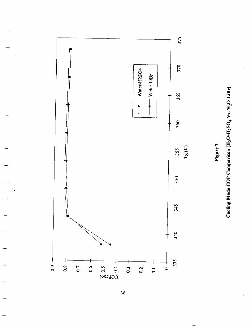
The cooling-mode COP of the water-sulfuric acid system as shown in Figure 7,

increases from 0.788 at Tg = 373K, to a maximum of 0.805 at Tg = 353K, and then

decreases rapidly. For the same range, the COP of the water-lithium bromide system

increases from 0.801 at Tg = 373K to 0.817 at Tg = 353K, and then decreases.

14

For constantTg,To,Te,andTa,asthe specific circulation rate (F) increases or the

difference between concentrations _3 and _ 1 decreases, the COP of the system decreases.

In the present study, the increase or decrease in F does not provide any information about

the COP of the system. This is because Tg is not constant. For the water-sulfuric acid

pair the specific circulation rate increases rapidly from 4.341 kg/kg of vapor at Tg -- 373K

to a maximum of 110.6 kg/kg of vapor at Tg = 338K. The increase in F is due to the

difference between _3 and _1 as a function of Tg. The change in specific circulation rate

as a function of temperature for both systems is plotted in Figure 8.

The maximum cooling mode COP is obtained when Tg is around 353K. The

cooling mode COP is the ratio of the heat absorbed at the evaporator to that supplied at

the generator. With an assumed constant load, the heat absorbed at the evaporator (Qe)

does not change and, therefore the only variable is the heat supplied to the generator (Qg).

Qg depends on several factors. As seen from Equation 8, h2, h3, m3, and m 2 are the key

parameters that affect Qg. Qg decreases as h3 decreases and h 2 increases. As Tg

decreases from 373K to 338K, both h3 and h 2 decrease. The ratio ofh 2 to h3 is largest at

a generator temperature of about 353K; hence the COP is maximum.

A plot of the heating-mode COP as a function of the generator temperature is

shown in Figure 9. For the case of water-sulfuric acid, the COP increases from 1.788 at

Tg = 373K to 1.805 at Tg = 353K, and then decreases. Similarly, the COP of the water-

lithium bromide system increases steadily from 1.801 to 1.817 for the same temperature

range. The increase in COP in the former case can be explained by the continuous

increase in heat of dilution evolved at the absorber, Qa- This heat is largely affected by the

enthalpy of the weak solution entering the absorber. On the other hand, as the

temperature lift decreases, Qa increases, and hence, overall COP increases.

15

AHP Performance using the Water-Magnesium Chloride Pair

The performance of water-magnesium chloride as an alternative refrigerant-

absorbent pair is summarized in Tables 11 and 12. The temperatures for the performance

calculation are Ta=298K , Te=283K ' and Tc=298K. The generator temperature varies

from 321K to 315K. The concentration of the strong solution leaving the generator (_3) is

greater than that leaving the absorber (_1)- This limits the range over which Tg can be

varied. The maximum temperature of the generator is limited to 321K, since the generator

and condenser pressures must be equal.

Table 11 shows the results obtained using water-magnesium chloride as the

working pair. The performance of this pair is compared with those obtained using water-

lithium bromide for the same heat pump conditions. The results of the water-lithium

bromide pair are shown in Table 12. The cooling COP of both pairs are compared in

Figure 10. In the cooling mode, the COP of the water-magnesium chloride pair remains

steady at 0.76 over the entire range. The COP using water-lithium bromide decreases

slightly from 0.904 to 0.794 for the same range.

Figure 11 shows the comparison of the specific circulation rates. As can be seen,

the specific circulation rates increase with decreasing temperature lifts. The sudden

increase in F for water-magnesium chloride is due to the appreciable change in mass flow

rate at the absorber outlet (ml). The only disadvantage with higher specific circulation

rates is that more solution must be circulated per unit mass of the refrigerant.

The heating mode COP of both pairs are shown in Figure 12. The COP for water-

magnesium chloride remains nearly steady at 1.76, while that for water-lithium bromide

decreases from 1.904 to 1.794. The water-magnesium chloride COP remains constant

because Qc, Qa and Qg do not change appreciably.

16

Conclusion

The AHP analysis has resulted in the discovery of some interesting features of

water-sulfuric acid and water-magnesium chloride as refrigerant-absorbent pairs, as

compared to the water-lithium bromide system. These are summarized as follows:

1. The water-sulfuric acid pair can be used as a satisfactory replacement for water-

lithium bromide pair in the targeted temperature range.

2. Unlike the water-magnesium chloride and water-lithium bromide pairs, the water-

sulfuric acid pair does not undergo crystallization.

3. The corrosiveness and toxicity of sulfuric acid must be taken into consideration in

the design of a practical heat pump.

4. At lower temperatures, the performance of the AHP using water-magnesium

chloride does not compare well with those obtained using water-lithium bromide.

5. The operating temperature and concentration ranges for the water-magnesium

chloride pair are limited by its solubility.

6. The computer codes developed can be used to analyze the performance of an AHP

with any refrigerant-absorbent working fluid pair with only slight modifications.

The results of this study should help future researchers to design more efficient

absorption heat pumps.

17

References

Alefeld, G. (1987). What needs to be known about working fluids to calculate

coefficients of performance. Heat Pumps: Prospects in Heat Pump Technology_ and

Marketing (Proceedings of the 1987 IEA Heat Pump Conference). Michigan: LewisPublishers, Inc.

ASt-IRAE Handbook: 1985 Fundamentals. (1985). Atlanta: American Society ofHeating, Refrigerating and Air-Conditioning Engineers, Inc.

Bhatt, M. S., Krishna Murthy, M. V., & Seetharamu, S. (1992). An absorption-

compression heat pump with the new working pair R22-NMP. Recent Research in

Heat Pump Design. Analysis, and Application, ASME, AES-28, 27-42.

Garimella, S., Christensen, R. N., & Petty, S. E. (1992). Cycle description and

performance simulation of a gas-fired hydronically coupled double-effect absorption

heat pump system. Recent Research in Heat Pump Design, Analysis, and Application,ASME, AES-28, 7-14.

Kaushik, S. C., Gadhi, S. M. B., Agarwal, R. S., & Kumari, R. (1988). Modeling and

simulation studies on single/double-effect absorption cycle using water-multicomponent

salt (MCS) mixtures. Solar Energy, 40(5), 431-441.

Lu, D. C., & Lee, C. C. (1991). Heat transfer correlation for condenser design in heat

pump. Recent Research in Heat Pump Design, Analysis, and Application, ASME,AES-28, 89-95.

Mansoori, G. A., & Pate, V. (1979). Thermodynamic basis for the choice of working

fluids for solar absorption cooling systems. Solar Energy, 22, 483-491.

Mayrath, J. E., & Wood, R. H. (1983). Enthalpy of dilution of aqueous solutions of

Na2SO 4, K2SO4, and MgSO 4 at 373.15 and 423.65 K and of MgCI 2 at 375.15,

423.65, and 472.95 K. Journal of Chemical and Engineering Data, 28, 56-59.

Mernik, B. D., & Mel'nikov, E. B. (1970). Technology of inorganic compounds.

(Kondor, R., Trans.). Jerusalem: Keter Press. (Original work published in 1968)

Patil, K. R., Tripathi, A. D., Pathak, G., and Katti, S. S. (1991). Thermodynamic

properties of aqueous electrolyte solutions. 2. Vapor pressure of aqueous solutions of

Na.Br, NaI, KCI, KI, RbC1, CsCI, CsI, MgCI2, CaCI2, CaBr2, CaI2, SrCI2, SrBr2,

SrI 2, BaCI 2, and BaBr 2. Journal of Chemical and Engineering Data, 36(2), 225-230.

18

Perry, J.H. (Ed.). (1950)...Chemicalengineers' handbook (3rd ed.). NY: McGraw-HillBook Company.

Perry, R. H., & Chilton, C.H. (Eds.). (1973). Chemical engineers' handbook (5th ed.).NY: McGraw-Hill Book Company.

Sako, T., Hakuta, T., & Yoshitome, H. (1985). Vapor pressure of binary (H20-HCI ,-

MgCI2, and -CaCI2) and ternary (H20-MgCI2-CaCI2) aqueous solutions. Journal of

Chemical and Engineering Data, 30(2), 224-228.

Serpente, C. P., Perez-Blanco, H., & Seewald, J. S. (1992). A single effect absorption

cooling machine with solution cooled absorber. Recent Research in Heat PumpDesign, Analysis. and Application, ASME, AES-28, 1-5.

Smith, J. M., & Van Ness, H. C. (1975). Intoduction to Chemical Engineering

Thermodynamics. Tokyo: McGraw-Hill Kogakusha, Ltd.

Snipes, H. P., Manly, C., & Ensor, D. D. (1975). Heats of dilution of aqueous

electrolytes: Temperature dependence. Journal of Chemical and Engineering Data,20(3), 287-291.

Soo, S.L. (1958). Thermodynamics of Engineering Science. NJ: Prentice-Hall.

Stoecker, W. F., & Jones, J. W. (1982). Refrigeration and Air Conditioning. NewYork: McGraw-Hill Book Company.

Warder, G. R., Annamalai, S., Nguyen, T., & Lin, C.H. (1993). Water/sulfuric acid as

refrigerant/absorbent fluid pair for the absorption heat pump. ASME Winter AnnualMeeting.

19

_Um

I...

0o_

I_I_@

@

!_

rJ_

m

0

i

<II

0

II

Jl [I _'_ _

_ _-.g

_+_,_ __

_-_" _ _._

20

©

O

Oo_

_q

r_

oa,u

Oom

O

O

.o

No

ra¢_

O

!

O

O

oN

O

!

lU!Od Su!zo_ad

21

e_

oom

m

o

om

i-

N

L

t-

oM

0

m

°_N°m

o

oM

II

>

0 "" _ ""

.__ .o ._= o

O O

N _ _ N

E EII II II II

22

o

0o

I I I I I

0O0

o o o0 0 O

o _ o

gl!l!lrl0A o^!J,rl0_I

00o

0

oO_

0o

oo

t'_

g_E

o

0

o

O

0m

II

o0_

o

0

I

0

0

0

.._el

23

rq

II II

iI

I

Iu

rq

li

I I I I i

0 0 0 0 0 00 0 0 0 0 00 0 0 0 0 0

•_l!I!lrl0A a^[lrl0"8

O

O

tt'300

o

t_.

g.*

o

E

O

a_

om

O-I

g_O

o_

or_

O

I

O¢'4

O

.m

m

O

24

.0

I_

o =oJ m

o

L.

L

E

!

2S

0°_

o

o

oo_

ell

0

J

J

o

E

E°_

o

vl

--, t'_

° ff•-_ _

o EE _

o_ _

I

+ _,iJ _

I ,-4

en II

%_._

_al _ t

II II II

26

00

0o_

0

om

0

0

Jm,!Nam

mo

0mM

27

00o

I I I I I l

0 0 0 0 0 00 0 0 0 0 00 0 0 0 0 0

Xl!l!l_IOA 0^p,el0_/

OOo

Ot._

O

t_

o

[-.,

O

O

t"q

oc'q

I...

0m

t...

t_

OomI-

OIm

No

O

!

O

o

_mNom

mO

*ml

m

28

N

=o

=No

r._

oN

r,.joII

_E

O

I_.OI=.

v3 00,q-

00O ,--,O

C50_ I

II OO II

-G

m _

,o _m Ed _ "-' _ Vl

I r,j" vl d

_ O

+ + + _-m _ ,_ _ _

+ _ _ _,o _ ,,, _ _ o+ + + c__

"_ II II II . ,-_ 0", _ _ 0II _0 I I

_0 Jl

29

N

0-,=

O

L_

eq

o

I

_0oo

(',,10

I

II

t-- VI("-1

_ _ Vl

d

Vl 0

m _ _ E+ + _

I '_ ,_, o

E + II fl

_ I-_ _1 0

E o .=

< II u_ o _o. ,__ 0

"Z

3O

[_

@,m

@

IIE_

_.. II0

("4

I Vl

o = II ,-_ Vl

+ _" _ _ o :_o _ _ _ _ vi _+ [_ • _ _ [_ ,_

o-j, a, _ o o

+ E _o_ _:; °° a_ o _ o

o_ + o _ _ o+ o c_ o_ it o _ _

o- o_r..T..l_ I ..:::_ o_ _,.,+ + ,-., ,-.,

o_ _ _ _ o o ._

+___ "_-o_ o_ o _ _. _ _ EII II li II _I .-_ II II li

31

m

oom

o

_S

÷

F_

U_÷

÷

E

F_

!

_o U_ _

oo0 . O0

II II II II _ oo

_ 0 e_l _'_ _0 _

II ,_,_ ,_-_ II II II II II II ,_ II II II

kid

VI

_ VI

I_ v_ o_. [_

VI _(_

32

I!

I

II

ol

I_Jnss_J d

L.

om

o

_tt=

o

t_

=

@

t..o

.<

33

_0

o...

_.,II

0J

oo on oo cq v'_ c.,I e_ _--oo _'_ o% 0 0 0, oo ,-,_.. _- L'-- oo oo oo t'-- _'_

I

_00 C_ 0% 0 0 0 O0 ,-'_t'- _- t"- O0 O0 O0 P'- _

_l_'_ _ +°_

_" _°I_ _° _° _° __d'o'c_'c_o o:o o

O0 O0 O0 O0 O0 O0 O0 O0

c_ d o d!c_ o o o

!cq 0 c_ o_ cq c,_ v_..!_.._. _._._ _ _o_- ,_-,_-,_- ,_- _- _-,o

_- P'- _0 q:) %0 %0

34

[..) ..=0 00:.-q ,'-q ,-q Ox L."_O0 O0 O01C_O O0 O0 L'_ ,_"

• • o, .....

°_

r._ _ _

oE

00'00 O0 _0 O0 O0 _".. '_-• . ., ....

0 0 0 0 0 0 0 0

_"_ ('q ',,0 O00_ ,-', O_:)i on

....... d

, ,-, C_!'_" 0 0 0

o0 0 Cxl 0 u'_,O ,..--_

E_ o o d'd o o d d

O 0 O 0 O_O O O

o o cS!c_ c_ c_ d c_

C_ _ cq eq cq ('xl eq eq'c,,i cq_ _. _.._ _. _ _. '_

,_i,_ _ _ _ ,_ _ r--,

3S

c5 c5 c5 c5 c5

1003dOD

c5t'qc5 0

t_

0

0

0t_

0

0

em

!

0

0

!

0

0o_

,_m t_

o

0

No0

36

000

I

0_0

0

_0

0_0

0

o'1

0

t I I I I I I

0 0 0 0 0 0 0 0

Oode^ jo _IN_t) :I

[...

o_

0i- r_

I_ eqD

oIm

"t-

37

0

0

0

oN

"C

=

0

!

0

0

S0_J

0¢J

tm

38

"0• -, II

o

0

_,_ _ > 0 0o %0 0% 0 "_- °°

o o c_ o o c_ c_

o c_ o c_ c_ c_ c_

(_ _ Cq_C',l Cq Cq C-_ Cq Cq

I •

39

eq

N

[-.ol, U •

°" II

o

oo °

o'%

o

E

O _ OO I" %0 0'

O_ C5._ 00 OO ¢_ t-

'_1" en t',l I'-- O_ _" _'

O_ O% O% _,oo oo,t'-

O O O O O O O

•"_ _ O O on O

v._ .--, _O ¢',1 i--- en O

.-'..-_ .-_ C',l o'1%O

_ O %O I'- O .--.

oo O _"'O _,%'O e,I

O _D O_ oo I'-- t',- _

O O O O O O '_-

ooooooo

(_ _ ¢',1 ¢',1 ¢'q ¢',1C',l t'4 ¢-,I

O_ O ,'-* P"- .'-_ OO v',P'- OO_OO OO'O% 0% on

O"1 r'_ O'1 0"% ¢_ 0%

0_,0_ _ e41_ _ ,-4

oo O_ O %o O _- en

¢_ o'1 ¢,1 t_ o"1 t_

40

6 d

0_ a.)

I I I f

c5 c5 o c5 o

10o_do3

I

,"" 0

0

¢xl

0¢'4

!

m

!

¢)

L. 0

,m

S0

0

0

oo

41

0

[...,

I_

ml

8

am

_60_

elm

0Q_

42

I

' I

4

¢

I i

l("4 oO _.0

¢q

I

o o

I I I I I

.- .- c5

l_0qdOD

¢xl

0eq

t_ _0

I t .-

.mI

¢q

I

¢)¢q

0

o

0

43

Section II

Design of an ElectroHydrodynamic Pump for the Absorption

Heat Pump

Design of an ElectroHydrodynamic Pump for the Absorption

Heat Pump

Introduction

Several thermal control techniques have been developed for thermal transport and

heat rejection in space applications (Kerrebrock, 1986). One method is the absorption-

cycle heat pump system. It is generally understood that the absorption heat pump offers

significant benefits in terms of mass and complexity reduction of the radiator area, tighter

thermal control, and relatively high efficiency. One essential component of the absorption

heat pump is a highly reliable pump which is needed to circulate the working fluids.

However, major problems limiting the reliability of currently used pumps include wear in

the bearings, seals, and in moving parts of the pump. The electrohydrodynamic (EI-ID)

pump is an innovative technology which, through proper development, can provide a

solution to this problem.

As early as 1937, J. Hartman and F. Lazarus investigated the EHD flow of

mercury between two flat plates assumed infinite in two dimensions (Samaras, 1962).

This fluid flow arrangement, known as Hartman-Poiseuille flow, was used in the

theoretical development of C. Beal (1967) and J. Melcher (1981). Since the work of

Hartman and Lazarus, several types of EHD pumps have been studied (Baker, 1987), but

the most appropriate type of EHD pump for aqueous fluids to date is a conduction, or

direct-current Faraday type. Also called simply an electromagnetic, or "EM" pump, this

type works on the principle of current flow across the fluid perpendicular to an external

magnetic field. A resultant body force is exerted on the fluid in a direction mutually

perpendicular to the current and to the magnetic field in the sense of a left-handed

coordinate system.

44

Liquid metal EM pumps based on this principle have been available since the early

1950's and are used primarily in nuclear reactor cooling facilities. Pumps of this type have

been built for volumetric capacities as high as 3500 m3/hour and for heads approaching

2.4 X 105 Pa (Andrev, 1981).

Investigations are currently being conducted by others on the use of

electrohydrodynamic pump for sea water thrusters (Doss, 1992). Also, this unique pump

is under investigation by the U.S. Navy for the development of a silent submarine

propulsion system (Swallom, Sadovnik, Gibbs, Gurol, Nguyen, van den Bergh & Hugo,

1991).

The EHD pump is considered to be a reliable means of circulating the working

fluid in a heat pump system because it has no moving parts, seals, or bearings. In a pump

of this type, the pumping force for moving the fluid does not originate from a piston,

diaphragm, or impeller. Instead, the force is exerted directly on the fluid. The EI-tD

pump, therefore, offers great promise for application in an absorption heat pump system.

Furthermore, the added feature of being able to repair or service these devices without

breaking the fluid circuit makes this pump more attractive than conventional pumps.

45

Theoretical Modeling of an EHD Pump

A continuum model is used to describe the characteristics of the END pump,

according to the following assumptions:

1. Incompressible, viscous, steady, and fully developed flow.

2. Uniform electromagnetic field applied in a direction perpendicular to the flow.

The physical configuration is illustrated in Figure 1. The governing equations for

the fluid, in normalized form (Melcher, 1981) are as follows:

V.fi=0(1)

at (2)

V x_ = 5__-a(_.x9 x_) (3)

-- + 9 • VV + VP = ----(_. + 9 x _) x fi +--V29 (4)at xM_ zM_ Xv

V.9=O, (5)

where, H, E, V, P, and t are electric field intensity, magnetic field intensity, fluid velocity,

fluid pressure, and time, respectively. The characteristic times:

1 rl 2

u' % = -- (6)rl

: Oo ol', : 'x- (7)

are, respectively, the transport time, viscous diffusion time, magnetic diffusion time, and

the magneto-inertial time. 1 is the characteristic length, U is the typical material velocity,

p is the fluid density, and rl is the fluid viscosity. It is assumed that the fluid is an ohmic

conductor with characteristic conductivity of Oo and essentially the permeability of free

space, po.

46

In typical laboratoryexperimentationinvolving the EHD flow of electrolytes,

liquid metals,or plasmas,themagneticdiffusiontimesareshort comparedto the time of

interest (e.g., xm<<x ). Hence, the magnetic Reynolds number (R% = x,/x) plays

almost no role in most parts of the flow regime. It is, therefore, appropriate to assume

that the induced currents on the right-hand side of Equation 3 are negligible. The

magnetic field is imposed by means of currents in the external windings. With the above

assumptions, the governing equations are reduced to:

Vx_. = o3_c3t (8)

V • 3 = 0; J = o(_, + _" x laoH) (9)

P(_tt + (9 • V)9) + VP = 3 x lao_ + rlV29 (I0)

Locally, the axial variations of electric field and current density are assumed to be

negligible in comparison with their variations perpendicular to the flow. This assumption

may not be accurate when strong variations exist in the magnetic and/or velocity flow

field, or when abrupt changes in the boundary conditions occur, as may happen near the

pump entrance and exit. However, this analysis is limited to the steady and fully

developed section of the flow.

For the task of finding a two-dimensional, steady-flow solution, Equation 10 reduces

to

_Vy c_Vy o (_toH o )2 Vy _ l-tooH o Ez + 1 dP (I ])C3x2 + D z2 11 11 11 dy"

The boundary conditions of this flow require that the velocity of the fluid be zero

at the fluid/wall interface. The volumetric flow rate Q is calculated from:

Q- j"vy oAe

(12)

47

whereAt; is thecross-sectionalareaof thepump.

Theelectricalpowerappliedto thepump(Pelec)is obtainedfrom

v._, c = J" (3 • _,)dV, (13)V

where V is the active volume of the pump. Since some part of the electrical power is

consumed in Joule heating, the mechanical power delivered to the fluid is, thus lower than

the electrical power applied to the pump. The power imparted on the fluid (Pfluid) can be

determined from

Pfluld = ; (F " "_y)dV, (14)V

where _ is the Lorentz force defined as _ = (3 x §). The actual power produced by the

pump (Pout) is calculated from:

yout = Q. Ap, (15)

where AP is the differential pressure across the pump. The actual power produced by the

pump is lower than the power imparted on the fluid due to the fact that some of this

power is dissipated as internal viscous loss.

Three different types of efficiency can be defined to provide an insight into the

behavior of the pump. They are:

1. Electrical efficiency, defined as:

(P • 9)dV

1]el,c = Pnuld _ v

v._,c ; (3 • P.)dV (16)V

2. Internal efficiency, defined as:

Pout Q. AP_]int --

Vt_id f (F. _)dV (17)V

48

3. Overall efficiency, defined as:

Pout Q- AP

P'"_ S (J " _.)dVV

-- _int • T]ele c

These three efficiencies are discussed in detail in later sections.

(18)

49

Numerical Method

m

Referring to Equation 11,

+__:_ Oz'

4- m

1 dP

rl dy'(11)

with Dirichlet boundary

face.). This equation can

(12)

technique is developed in

1/2, and z = -w/2 to w/2,

,d, the finite difference

h2k2), (13)

t is then utilized with this

iterations required to

ly reduced. The algebraic

i,j = (1 - to, i,j + i,j. (14)

and v _k,= 1 ,v ,k-l,v _k" _, _-I" ,_i,j 4 + h2kx ' i+1,j + i-l,j + "l,j+l -1" Vl,j_ 1 -- h2k2), (15)

where:

Vi, j is the velocity calculated from Gauss-Seidel iteration at node i, j

Vt, j is the approximation of Vy by the SOR method at node i, j.

to is a relaxation parameter.

<k> is the component of the k th iteration.

The optimal value of the relaxation parameter, co, is found empirically by

performing calculations with different values of co for coarse grids until the optimal value

of to is obtained. With the optimal co, the corresponding optimal value of co for finer

grids can then be found by applying the following formula (Strikwerda, 1989) •

2O --

1 + ch (16)

where C is a constant obtained experimentally, and h is a distance between iterative nodes.

A computer program (Appendix B) was written to implement the iterative scheme.

Numerical results from this program are then transferred to a graphics software package

for graphical presentation.

51

Experimental Apparatus and Instrumentation

Experiments Were performed to verify the theoretical results obtained from

modeling the electromagnetic flow. A copper sulfate solution was used as the working

fluid for model verification, with properties as shown in Appendix B.

.Experimental Apparatus

The experimental apparatus, illustrated in Figure 3, consists of a reservoir,

rectangular conduit, EHD pump, manometer, rotameter, and secondary centrifugal pump.

As can be seen from Figure 3, the rectangular conduit carries the fluid from the

reservoir to the EHD pump, and is connected by the return conduit (7.875 mm ID). The

flow rate was monitored by a rotameter connected to the end of the return conduit. A

valve at the rotameter was used to control the flow rate of the system. The secondary

centrifugal pump was connected from the reservoir to the rectangular conduit in parallel to

the direct connection between the reservoir and the rectangular duct. This secondary

pump was used to drain air bubbles from the system during the startup process. Startup

and operational procedures are discussed later in this chapter.

The rectangular conduit, with internal dimensions of 6.35 mm by 25.4 mm, was

made of Plexiglas. Plexiglas was chosen because, in addition to being a good electrical

insulator, it also allows visual observation of the pumping process. The various Plexiglas

parts were assembled using dichloroethane solvent.

Two 6.35 mm by 101.60 mm slots were provided on each side of the conduit at

the pump section to accommodate the copper electrodes, which were affixed to the

Plexiglas conduit with epoxy.

Figure 4 illustrates the EHD pump used for the experiments. The EHD pump

envelope is by definition the volume between the electrodes and the magnetic poles. Some

52

considerationwas given to the fact that the theoretical modeling was based on the

electromagnetic flow in the fully developed region. The pump section, thus, should be as

long as possible to comply with the theoretical model. The length of the pump section

was chosen to be 101.6 mm (four times greater than the width of the channel).

The copper electrodes, shown in Figure 4, were connected to the power supply via

three #18 AWG insulated wires to ensure even distribution of the electric field across the

pump section. The surfaces of the electrodes were sanded and polished before installation

in the conduit. A 15 ampere, 0-50 volt DC power supply (Accurate Electronics Co.,

model PP-1725) was used with the electrodes.

The magnetic circuit was designed to provide a maximum of 0.4 teslar magnetic

flux density in the vertical direction across the pump section. The geometry of the steel

core and the arrangement of the coil winding were configured to minimize magnetic

fringing outside the pump. Figure 5 illustrates the details of the electromagnet used in the

test setup.

Since a larger wire requires higher current at lower voltage and vice versa, an

analysis (Appendix C) was performed to select the proper wire size for operation at the

voltage and current rating of the available power supply. According to the analysis, #18

AWG wire with 840 turns is sufficient for this application.

A 10 ampere, 0-55 volt DC power supply (Epsco Incorporated., model PS-5) was

used for the electromagnet power supply. The actual magnetic flux density was measured

using a gaussmeter (General Electric, model 416X37). This reading was then used as a

standard for the entire set of experiments. Comparison of the calculated and measured

magnetic flux density is given in Appendix D.

A manometry system was used to measured the difference between the suction and

discharge heads. Two static pressure taps of 2.23 mm diameter at the entrance and exit of

53

the EHD pump were connected to the manometer tubes (glass tubes of 4.5 mm internal

diameter) by 3.175 mm internal diameter flexible plastic tubing.

The flow measurements at high flow rate were acquired using a Dyna VFB-141-

BV, 0.5-5 gpm (31.5.10-6-315.4.10-6 m3/s) rotameter. The rotameter was calibrated for

the test fluid (Appendix E). To obtain accurate readings at flow rates lower than 31.5.10-

6 m3/s, the flow measurements were made by measuring the total volume collected in a

given time interval.

Initially, a pitot tube was installed at the end of the pump to measure the local

velocity of the fluid. However, this method was abandoned due to unsatisfactory

differential pressure measurement.

Two multimeters (Micronta Electronics Inc., model 22-185A) were used to

measure the voltage and current applied to the electromagnet and electrodes before each

experiment was performed. Once the experiments were started, the voltage and current

readings were then monitored using the voltmeters and ammeters provided with the power

supplies.

Exoerimental Procedure

Atter apparatus assembly, leak-checking, and instrumentation verification, the

experimental system was certified "test-ready," and all was in order to begin the test runs.

Before beginning, however, some precautions were taken to assure the integrity of the test

data. These are summarized as follows:

1. The valve at the rotameter must be fully opened when the centrifugal pump is

turned on in order to prevent hydraulic pressure from building up and rupturing the

conduit.

2. Prolonged use of the electromagnet may cause a damage to the magnetic circuit

due to high temperatures generated in the interior coils. Thus, coil temperature was

54

gaugedby noting the rising resistance of the magnetic circuit. In this way the resistance of

the magnetic circuit was monitored continuously and maintained lower than 6 ohm during

the experiments.

3. The resistance across the electrodes must be regularly monitored. If the

resistance is higher than the initial value (8.8 ohm), the electrodes must be cleaned. This

increase in resistance cross the electrodes is due to the uneven deposition of copper and

impurities on the cathode.

After having incorporated the above precautions into the test operation, the

following experimental procedure was implemented:

1. The test loop was filled with the test solution. This was done by pouring the

test solution into the reservoir until the level of the test solution was approximately 10 cm

above the conduit level. The valve at the rotameter was then slowly opened to allow the

solution to flow into the conduit. Trapped air inside the conduit was drained by closing

the ball valve located near the reservoir and turning on the centrifugal pump to help

circulation and to force air to exit the system at the reservoir.

2. The magnetic circuit was energized. Multimeters were used to monitor the

current and voltage applied to the electromagnet. The supply source was adjusted until

the power necessary to provide the desired flux density was obtained. The power supply

was then turned off.

3. The power supply to the electrodes was turned on. The power supply was

adjusted until the desired voltage across the electrodes was obtained. Two multimeters

were used to monitor the voltage and current supplied to the electrodes during this

process. The power supplied was then turned off after the desired power was set.

4. For each position of the valve settings at the manometer (from fully-closed to

fully-opened), the magnetic field and the electric field were simultaneously energized. The

ball valve at the reservoir was then opened. The differential pressure head across the EHD

55

pumpwasmeasuredby themanometer..Thelower surfacesof the suctionpressureand

the dischargepressuremeniscusesformed in the manometertubeswere marked. The

height differencewas then recorded. The flow rate was also observeddirectly at the

rotameterfor high flow rates. For lower flow rates,wherethe rotameterreadingwas

inaccurate,the time intervalrequiredto fill a calibratedcontainerwas recorded,andthe

flow rate was calculated from this data.

5. The experiment was performed for various magnetic flux densities and voltages

applied across the electrodes. Table 1 summarizes the various conditions of magnetic flux

density and voltage across the electrodes used in the test runs.

56

Results and Discussion

Numerical results

The following sections discuss the numerical results obtained for the velocity

profile, pressure-flow rate relationship, and efficiency of the EHD pump as a function of

magnetic flux density and conduction current.

1. Numerical Results for the Velocity Profile

The numerical methods developed earlier have been used to determine the flow

characteristics of the EHD pump. The numbers of nodes in the x and z directions were

initially chosen to be 11 and 41, respectively. The dependence of the accuracy of the

results on the number of nodes chosen was then investigated. It was found that the results

varied by less than 1% when a 21 X 81-node configuration was used, and more than 3%

for a 5 X 17-node configuration. Hence, the 11 X 41-node configuration was retained for

this analysis.

The relaxation factor (co) is an empirically determined quantity of the calculational

process. Since the solution converges rapidly, the relaxation factor can be found directly

without using the scaled-down configuration (lesser number of nodes). It was found that

the most suitable value of the relaxation factor for the nodal configuration used (11 X 41)

was 1.7.

Since the mathematical model has no closed-form solution, verification of the

results was accomplished by modifying the two-dimensional finite-difference scheme

developed earlier to a one-dimensional model, and then comparing the results obtained

with the analytical closed-form solution. Comparison of the numerical and closed-form

solutions indicated an error of less than I%.

57

An exampleof thenumericalresultsobtainedfor theaxial,fully-developedvelocity

profile is shownin Figure 6. The vertical plane indicatesthe axial componentof the

velocity(Vy).

TheLorentz force in the axialdirection(JzX B) actsasthe driving forcefor the

pump. This force,however,is notuniformover the entire cross-section of the pump flow

area, due to the non-uniform distribution of the current density. It can be seen from

Equation 7 that the local current density depends upon the local fluid velocity. For an

EHD pump, a higher fluid velocity corresponds to a lower current density. The force

acting on the fluid near the walls, where the local velocity is lower, is higher than that at

the core of the duct. This increase in the force causes a rapid change in the velocity

profile near the walls.

From the above discussion, it appears that two factors, namely, the voltage across

the electrodes and the magnetic flux density, are the parameters controlling the

characterization of EI-ff) pump performance. Figure 7 (a,b and c) illustrates the resultant

velocity profiles for various applied voltages with constant magnetic flux density and

pressure. The voltage across the electrodes exhibits a synergistic effect on the velocity

profiles as indicated in the figures for voltage variations from 10 V to 20 V. In Figure 8

(a, b and c) , the effect of varying the magnetic flux density is shown. As with the

previous case, the velocity profiles intensify as the flux density increases from 0.2 T to 0.4

T.

2. Numerical Results for Pressure-Flow Rate Performance Characteristics

The pressure-flow rate relationship is also of primary interest in characterizing the

performance of the pump. A parametric study was performed by varying the differential

pressure while the pump power input was held constant. The analysis indicates that the

theoretical pressure-flow rate relationship for an EHD pump is similar to that of a

conventional centrifugal pump.

58

Figures 9 illustrates the pressure-flow rate performance characteristic for various

magnetic flux densities with constant voltage maintained across the electrodes. As

indicated in the figure, an increase in the flux density increases the pump output.

The effect of the voltage applied across the electrodes on the pressure-flow rate

performance characteristic is illustrated in Figure 10. As can be seen from this figure, the

pump output increases with an increase in the applied voltage. However, it should be

noted that the physical properties of the fluid limit the voltage across the electrodes. This

limitation is discussed later in this chapter.

3. Numerical Results for Pump Efficiency

Since efficiency is a parameter of primary importance in characterizing the

performance of an EHD pump, the efficiency was determined using two different

methods.

In the first approach, the effect of magnetic flux density and voltage applied to the

electrodes on pump efficiency was investigated while maintaining a constant flow rate.

This method is useful in determining the optimal input condition for a given flow rate.

In the second method, the effects of flow rate on pump efficiency were studied for

a given voltage and magnetic flux input. This method provides a convenient way of

comparing the numerical results with the experimental results. The comparison of the

numerical and experimental results are discussed later in this chapter.

i. Effects of Magnetic Flux Density and Voltage Across the Electrodes on EHD

Pump Efficiency.

Three different types of efficiencies have been previously discussed. Figure 11

illustrates the effects of the magnetic flux density and the voltage across the electrodes on

the internal efficiency of the EHD pump for a constant volumetric flow rate. As can be

seen from Figure 11, an increase in either the magnetic flux density or the voltage across

the electrodes increases the internal efficiency of the pump. This is because, at constant

59

flow rate, the viscousloss in the fluid .is almostconstant. For a higher magneticflux

densityor anincreasein thevoltageacrosstheelectrodes,thepumppowerinput increases

while the lossesremainnearlyconstant.This improvestheinternalefficiencyof theEHD

pump.

Theeffectsof varyingmagneticflux densityandvoltageacrossthe electrodeson

theelectricalefficiencyareshownin Figure 12. As indicatedin theFigure,highelectrical

efficiencycanbeobtainedusinghighermagneticflux densityandlower voltageacrossthe

electrodes.This phenomenoncanbe explainedby consideringlocal electricalefficiency

givenas:

[rl,l,C]1oc,I _ B.Vy _ B.Vy (17)E v/w

where B is the magnetic flux density; Vy the local velocity of the fluid and E the electric

field strength. E is again defined as the ratio of the voltage across the electrodes to the

width of the pump (E = v/w). For a given flow rate, the local fluid velocity is almost

constant. The local electrical efficiency thus depends on the ratio of the flux density to the

voltage across the electrodes.

It should be noted that the local electrical efficiency is not uniform over the entire

cross-sectional area of the pump. Equation 17 indicates that the local electrical efficiency

depends on the local fluid velocity. The local electrical efficiency of the fluid at the core

is, therefore, higher than that near the walls. Figure 13 illustrates the overall efficiency of

the pump. The overall efficiency of the pump is the product of the integrated electrical

and internal efficiencies. An increase in the magnetic flux density will increase both the

electrical and internal efficiencies, therefore increasing the overall efficiency of the EHD

pump. An increase in the voltage across the electrodes will increase the internal efficiency

but decrease the electrical efficiency. The maximum overall efficiency of the pump is

6O

therefore dependent on the particular pump configuration, namely, flow rate, voltage

across the electrodes, and magnetic flux density.

ii. Effect of Flow Rate on EItD Pump Efficiency

The effect of volumetric flow rate on the efficiency of the pump is another

important characteristic which must be understood to properly characterize pump

performance. A parametric study was conducted by varying both the volumetric flow rate

and the pump power input. Figures 14 (a and b) illustrate the relationship between

internal effÉciency and volumetric flow rate for various input conditions. As can be seen

from the figure, the internal efficiency decreases linearly from its maximum (no-flow

condition) to zero (maximum flow rate). This is due to the fact that the viscous loss of the

fluid is directly proportional to the volumetric flow rate. For the maximum flow rate, all

of the mechanical power delivered to the fluid is used to overcome the viscous loss.

Therefore, no useful output is produced. The internal efficiency of the pump is thus zero

for the maximum delivery condition. Since the viscous loss converges to zero as the flow

rate approaches the no-flow condition, the internal efficiency is at its maximum.

Figure 15 (a and b) shows the electrical efficiency-volumetric flow rate relationship

for the EHD pump. Increasing the flow rate results in an increase in the mechanical power

delivered to the fluid but does not change the input power to the system. Therefore, the

electrical efficiency increases as the flow rate increases.

In Figure 15a, it is important to note that as the magnetic flux density increases,

the slopes of the electrical efficiency-flow rate curves (each at a constant B) increase. But

as seen from Figure 15b, the slopes of the electrical efficiency-flow rate curves (each at a

constant v) decrease as the applied voltage across the electrodes increases.

Overall efficiency curves for the EHD pump are shown in Figures 16 (a and b).

The overall efficiency as defined earlier is the product of the internal and electrical

efficiencies. Figures 16a shows that for a given voltage across the electrodes, the overall

61

efficiencyincreases from zero to a maximum and then decreases to zero as flow rate

increases from the no-flow condition to the maximum-flow condition. As the flux density

increases, the maximum value of overall efficiency also increases. It should be noted that

the maximum values of the overall efficiency occur at higher flow rates when the flux

density increases.

Figure 16b shows the theoretical relationship between overall efficiency and flow

rate for constant magnetic flux density and varying voltage. For a given value of voltage

applied across the electrodes, the overal! efficiency increases form zero to its maximum

and then decreases to zero as the flow rate increases. As the voltage increases, the

maximum value of the overall efficiency obtained remains approximately the same but

occurs at higher flow rate values.

Experimental Results

Since repeated attempts to measure the velocity profile yielded unsatisfactory

results, the following sections will focus only on the experimental results obtained for the

pressure-flow rate relationship and efficiency determinations for the EHD pump.

1. Experimental Results of Pressure-Flow Rate Relationship

The effects of the magnetic flux density and voltage across the electrodes have

been discussed in previous sections. Figures 17 to 28 show the comparison between the

experimental and theoretical pressure-flow rate relationship for various input conditions.

The various input Conditions are summarized in Table 2.

As seen from Figures 17 to 28, the experimental values agree well with the

predictions for low flow rates. At higher flow rates, the experimentally measured values

were lower than the predicted values. The aberrations observed are due to the assumption

that the flow is fully developed. Since the fluid at low flow rate tends to become fully

62

developedfaster than the fluid at high .flow rate, the theoretically predicted values are

more accurate at the low flow rates than at the high flow rates.

The difference in the measured and predicted pressure at high flow rates may also

be due to the non-linear losses in the system. These non-linear losses are the those caused

by local turbulence.

For higher values of applied voltage across the electrodes, the efficiencies obtained

experimentally were lower than the predicted values. The variations observed were due

to increasing current fringing at higher voltages. This resulted in the decrease of the

useful conduction current in the system.

Physical properties of the working fluid also limit the applied voltage. High

voltage applied across the electrodes caused an uneven deposition of copper on the

cathode, thus increasing the electrode surface resistance. This effect degraded the pump

power output rapidly. Since this phenomenon is pronounced for applied voltages higher

than 20 V, no experiments were performed in this voltage range.

As the magnetic flux density increased, it was expected that the fringing effect

would cause variations in the experimental results, in the same manner that current

fringing did. However, comparison of experimental and theoretical data does not

conclusively substantiate this theory.

2. Experimental Results for Overall Efficiency

Since internal and electrical efficiency could not be directly measured, the overall

efficiency was the most important parameter of interest. The theoretical effects that the

magnetic flux density, the voltage across the electrodes, and the volumetric flow rate have

on the overall efficiency have been discussed previously.

The experimental and theoretical values of overall efficiency are shown in Figures

29 to 40 for the various input conditions. The input conditions are listed in Table 3.

63

As can be seen from Figures 29 to 40, the experimentally obtained efficiencies

agree well with the predicted values at low flow rates. However, the experimental results

were lower than the numerical results for higher flow rates. This is due to the fact that the

actual differential pressure across the pump is lower than the theoretical value, when the

flow rates become higher.

The current fringing effect could also cause the actual overall efficiency to be

lower than the theoretically predicted value. As discussed earlier, higher voltage across

the electrodes increases the current fringing, thus reducing the power output of the pump.

Although theoretically, the magnetic fringing should decrease the pump performance,

experimental data does not substantiate this fact.

64

Conclusions and Recommendations

An investigation of the operational characteristics of an electrohydrodynamic pump

was performed in this study. The numerical and experimental results obtained provide an

insight into the electrohydrodynamic characteristics of the fluid inside the pump. The

results obtained are summarized as follows:

1. The numerical mathematical model developed based on continuum

electromechanics provides reasonable results within the limitations of the assumptions

made.

2. The operational characteristics of the EHD pump as predicted by the model

were found to be similar to those of a conventional centrifugal pump.

3. The predicted overall behavior of the EHD pump is comparable to that of

turbomachinery hardware; however, the overall efficiency of the electromagnetic pump is,

as predicted, much lower.

4. The pressure-flow rate performance characteristics and overall efficiency of the

pump obtained experimentally agree well with the theoretical results.

Although the model developed during this study yielded satisfactory results, better

results could be obtained with a more sophisticated model based on a three-dimensional

mathematical model.

The small size of the experimental apparatus used in this study caused some

inherent limitations in the accuracy of the measured quantities. In the future, these

limitations could be eliminated by utilizing a pump of larger capacity.

The electrohydrodynamic pump is very sensitive to fluid properties. Because of

this, care must be exercised in selecting the feasible range of operational parameters and

appropriate electrode types for a given application. As a recommendation for future

65

research,it is proposedthat additionaleffort beexpendedto explorethe varietyof fluids

available,with appropriateelectrodecombinations,for usein anEI-IDpump.

Also, as the overall efficiency of the pump is largely dependent on the magnetic

flux density, superconductors could be used to improve pump performance.

The development of the EHD pump for circulating the working fluid in the

absorption heat pump system can be considered a high-risk, high-payoff application of

advanced technology to provide revolutionary improvement in reliability and

maintainability of the heat pump system. The results of the present effort should help

researchers understand the fundamental performance characteristics of this type of pump

in order to develop an improved electrohydrodynamic pump for future applications.

66

References

Ames, W.F. (1977). Numerical Methods for Partial Differential Equations. NY:Academic Press.

Adreev, A.M. (1981). The TsLIN - 3/3500 electromagnetic pump.

Magnetohydrodynamics, 24(1), 55-61.

Baker, R. S. (1987). Electromagnetic Pump Technology. NY: Elsevier Press.

Beal, C. C. (1967). A Study of the Macroscopic Performance Characteristics of a

Stesdy-State Electromagnetic Pump for an Electrolyte. Unpublished master's thesis,

Texas A&M University, College Station.

Guna, S. K., Alfred, W. R. & Benjamin, R. (1966). Pulsatile Electromagnetic Pump

Without Moving Parts. Medical and Biological Engineering_ 24(1), 53-67.

Kerrebrock, J. L. (1986). Optimization of Heat Rejection in Space. ,lournal of

Propulsion,2, 562-563.

Melcher, J. R. (1981). Continuum Electromechamics. Cambridge: MIT Press.

Samaras, D. G. (1962). Theory of Ion Flow Dynamics. NJ: Prentice-Hall.

Strikwerda, J. C. (1989). Finite Difference Schemes and Partial Differential Equations.NY: Wadsworth & Brooks/Cole Advancs Books & Software.

Swallom, D. W. (1991). Magnetohydrodynamic Submarine Propulsion Systems. Naval

Engineering Journal, 103(3), 141-157.

Warrier, G. R., Annamalai, S., Nguyen, T. & Lin, C. H. (1993). Water-Sulfuric Acid as

Refrigerant-Absorbent Fluid Pair for the Absorption Heat Pump. ASME WinterAnnual Meeting, New Orleans.

Woramontri, W. & Nguyen, T. (1993). A Novel Electrohydrodynamic Pump for the

Absorption Heat Pump. ASME Winter Annual Meeting, New Orleans.

67

\\

0

U

I

68

II

1

I ,m

G,m

°"

0

=,m

O

69

)

E

00 U

w

.J

m

_u_J

|

u

!

70

W

W

m_r_

w

k

om

_U

"C

M

0

71

_b

I

II

! !

|

Q_L

_Douu

_D

,o

q_mm

qbJ

0

72

eiI

el

0

L)m

r_I,)

Et_

q_

mo

r_

.m

r_

II

m

o.N

.mm

o

m

4_E

m_l,q

_p CO

•IJ .I-)

.M .M

I-I

J.)

)4

:#: :#: :_i[_.I-) ._

•,4-,_ E

"

c

o E E!-r.I .M

r_ u_ c

• r-I -r_ -i

X X

II II

?3

Q

,ml

mNml

Z

o_

0

o

omm

om

_m

o

m

mlM

74

a

l

cqJ_o

II

C_

II

o

_0

L

_om

,o

oN

0N

q_

75

q_(uIm

at

0

II

c_II

Q

II

Ii

_omu

0lu

om

0mu

q_

76

4

r

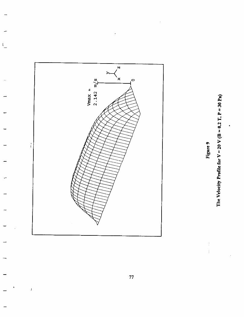
0

II

II

C_

H

am_omu

oLI

om

Omuq_

??

C_

II

fl

L

om J_

q_era1

0L

o

78

omm

c_

0

II

tt_lmq

II

II

L

_oG_

N

@L,

J_

@imf

[-

79

oN

0q_

N

vl

II

c_II

LI

L_N

oIi

oml

0m

$0

t-I

I I I

/s

/Lo,-4

/t

/r

/i

/

!s

/i

f/

e

'o

t

/

CD t

/

/s

/

ii

o

A

v

I, I /'

/ /' /

/ //

!/

!!

/!

/

rn !!

II i1 E-q

_ iI c_

i o

nI

I Io

M

-- r_ E

k,O

_0

i--I

r-r-- c_

0

tt

v-4

o

o

o

0

I

I.=

u

81

I i I I I

I 1 I

II

II

II

II

II

II

II

i I /

I ,'

e4 I

I _ /li / r'-t ,,

1/ II / 0,_1

/ _ /

/ /

! ,

/ /

// /

/ II/ ,

/ ,I i

I I

//

E

IDI

O

e-t

i t

/ OL

/ !

_N

8

N

o

@

i

L_

82

6

t

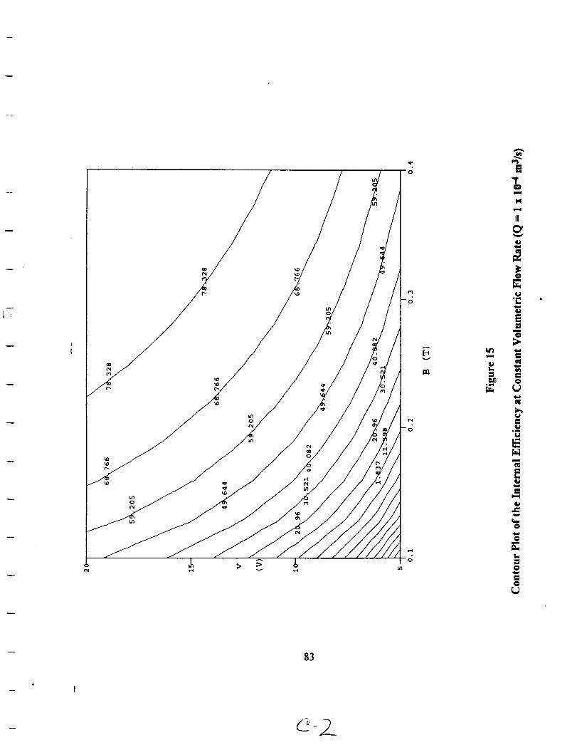
A

v

lm

1,4

_=

I:o

im

E

E

,,,1=

O

o

L.

o

or_

83

q*

v

m

o

L.

f?¢D

M

II

t:

Emm0

r_

o

.I

N

.11L.

M

.G

0

0N

o

[]o

84

t

v

_q

II

o

or"Q_

mo

Q_ cqr_

al

q_

E

qmUmc_Ii

q_P

rm0

0m

I.

o

o

85

I I I I

/

/

/

/

>

o ._'/

II

/

/i

,-I

/;II

7J

/

/ _ -• / I_

/ _ 0

/ // II

,/ //

/ // • _

.///

I I I I0 0 0 13

,-4 _j

opI

00qiq

Ou3

-- M

¢n

N m_v

_0

00

o r-Io

C_

o0

L

Qm

¢N

dII

om

Vq

om

O_J

N

_0¢q

O

om

O=O=

O

oom

e=

m

E

86

i

1

I I ' I /

I, /

o I

/ / -II '

_Im /t

i

/ o /' II ' /

/ _/ //

/ / _ /• /

/ / _ / /i

I , ///J

d / _" _• /

/ /

' / / • /

- 1 , // o /-, I / ,

,I i'. ///

- ,/ /' /// _ -

.'1,////

,I/ // _

g/ •I I I I0 0 O 0

0 _ _,O .lJ _1' 1",1

00

OO

M

o

IO

o

oLN

OO

v')

II

mo

o

M

o

o

<

G.m

E

87

B

I

\ I

\

\

\ \ 1(_

o \ II

o _ II

• \,

\ \

\ '\

\,\ '\

I I I I

oo _ A o o

A

_Ev

_D

no

C_om

II

JO

e_O

r_

o_

O

OQm

88

¢

0

II

::>

'\ I

\

',\

\\

\\

\

o

U

v

\

O

, II

\>

\

\

\

\

\ \\

\

\\ \

II

ol

1,4

tm

@

N@

Ol

OII

@

@oN

Ol

N

89

I

l

I V I I

i

/

o

;I

\

\

\

\

\

\

\

• f

°lII,

i

!r

/t

/

\

\

\

\

\

I I I I I

o

>

__o

/

/i

I •

/

//

I

II

I

I

o

o o o

o

Tl

\ o

' II\

\ \ \• \

\ \ \

"..%\

l

o o

o o o

l

o

'Oo°

C_

oi-I

e,l

i¢)

o

_Q

IB

O

0_N

_B

ol

l

>

9O

Q

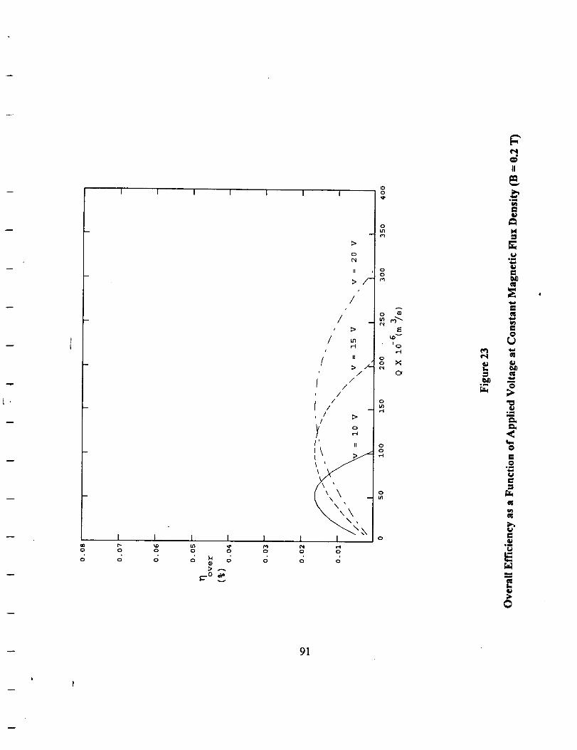
I I i i i I i

I

o

I 1 I i_D U3 _, M0 0 0 0

o o _ o o:> .-,

I

o

o

C'I

II 0

>/-

/

/ _

i

/ II

, /

I /, /

/f / _, /

/

y °e-.i

I' II

'X,. \\\

"-<.<.,,IrtQ

d

00_P

mrn_E

I 0

rl

o xCx

oLn,-4

O

Or'4

O

e_

L

Qm

O

II

e_

M

0_

G,)

eq

O

a

m

O

omm

O

Oom

om

N

O

91

I

I_ 0_

4

I_ _o,-I o,-I -,-i

m,.O

i_

OI_.

Oi_

Iu

MO

al

I,#om

Iu

r,'l ['_ _-I

IN I_D O

_-I 1.1"1 1.1_ I._

,,'ggg

O i.n o!-I ,-I

II II II

92

I I I I i I

?,

s,_

o

!

U_

s,_.

93

Q

1..,.,.

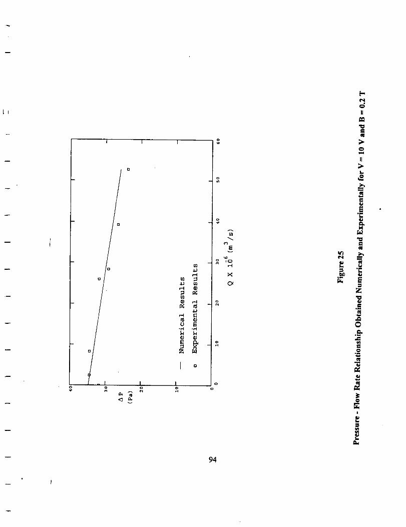
rd _LJ E

°,-q °,_

J Q

A

r_

Ev

_D

M° ,o

C_

o

94

om

c_II

at

0v_q

IJ

IN

_omm

°_

J_

mm

o_r_J

°_q_

lnu

c_

oN

0tIN

mu

0

!

r_r_

Tu

4

I I I I I

f

1 I I

.IJi-I

r-4

_J

Wu E

-H -r'l14 14

E _

I 0

1 I

_ °rt

-

_ ._

tn

, o

o

A

uJ

Ev

_)iC:)

I--I

C_

II

_Q

L.

•_ .

i

0

!

95

I I

O

-- O O

O

I

O

v

u)

r-_

4J m

m

_J

Wu E

or,t

I Q

_o

-

_o

o

o

A

M

E

iO

r_

C_

7,

t.

o

!

L

97

II,-, I n_, A_ °

I I c

Z _

I °

I I

II

i

i

III

° _O

I

98

I i I

0

i

I °I Io o_ _r

_ n5

II

c_

I..

,..o

o _.

_E c_

0.

oj:o

!

r_

99

I

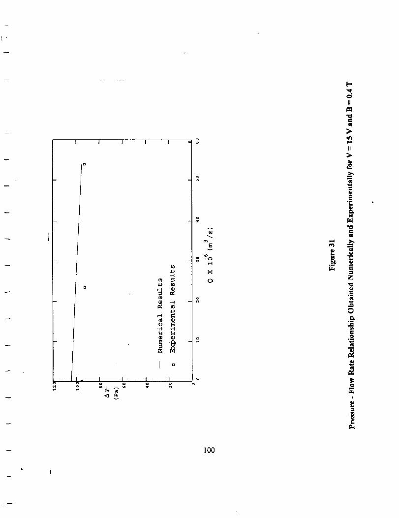
on

II

N

V')

II

N

E

mm

Iu

G,m

,M

0

0

!

lO0

I

0

0 0

u)

u)

U E•H -H

I D

o

M

E

X

C_

f_

.m

II

ell

O

II

I-

M

C

M

mm

E

0

oN

Ot_

m

0

!

L

101

Q

o

l O

O

m

.IA --

u-H -_

I O

o¢,1

A

o t_" E

v

00

or_

Ot

o

o

102

gi,

eq

I!

I:I

oeq

o

!

qh_a_

I_

II

L.

m

"r"

mM

"r'

im

om

.m

oom

m

I o I I i I

D °

_-_ _

u E-el -_

J D

1_ I' I I I

v

, o

o

If

"_ °

tD

@

!

103

II

' i iL

Z _a

I o

oo

!

104

t

e_

la

F,

0

O

om

r,r,wI,,,

la

0I=,

i

r*T*1

._e

m

0

INI

I=

r"-it-I u'l

,_ _ Lr) l.r)

r_ r_ _

i_ .,-i.,..i._r_ _ _

:E, c,lr,irn

. &&l&_ _ r_

,,_ c0 o

r_ r_ _

p, p,':>

0 un 0_-I ('_

II II II

105

o

o

w

0

0

I

o

o

I ] l

_J

m

m mE

E

f/l

tOIQr-t

M

0

L°o

[,,.

II

U

II

n.-

mm

0,

m

"=

S

Z

=IN

E

106

\ r-4 (19

_o _ _ -

u E-,-t .,-_

G) •

o

ul

o _

IO

X

0

o

o _0 o o° >0; °

oII

m

o

II

k,

m,u

S"C

t_ I,(

(I,)

: =

N

e_

o__J

E

0

107

i

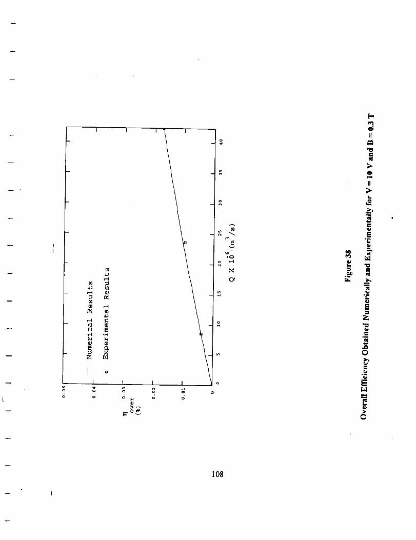
b"J4..3

co4.3 r,,/'J,--I _)

4-)

u E_-r4 -,Ht..i

I

I D

Io o

o o

o_

®

_..o_

0

II

0

II

L.

mm¢q

m"c

M

mm

r,a"E:

om

Im

mm

108

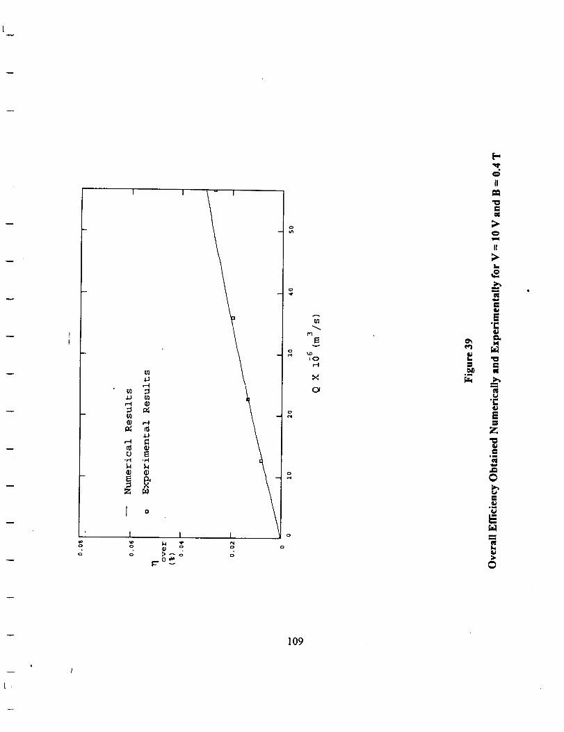
m

ou E

• •

J D

I

o

0_t_- _

o

o

A

ul

E

IOr-t

X

o

INIom

"t.0

IIm

0

II

mm

1,4

al

mN

.M

0

.N

mN

I._

0

109

o

(::)

I

o

- I I _ --

o _ _I

.I-}o _

I I I

0 0 0

A

m

E

IO

II

"O

N

II

L

Mm

'CD.

o

,m

mm

.N

o

°m

Em

110

I D

I- I

I I

oo Q) o

_..0 "pv

o

o

A

E

uO

X

ol

IIm

II

E

e_

E

Z

o_

Q

o_

E

q_

111

I I I

4-)r-q

_J

r-_

_J

u E-rl -r-I

E

I {3

I I I

0 0 _I 0

Q)

0

0

ul

ME

v

iOr-I

[-

0

II

ml

II

t..

Mm

tu

E

_ M

em

mm

-=

Z

em

0

4,)om

EI

0

112

t/l

r-.4m

O)

a_ m

t_ E-r4 -r4

E

f O

I I I

1,4

>AO_

o_o o

/

A

0)

o ME

v

IOr-4

t2_

ca

o

L.

II

g:

II

mM

g_

E.r"

M

mme_

om

E

mm

113

L

-H -H

0

I

o o

o o

I I

II

II

k

-r

M

I

°_

Z

O

E

k

0

114

I

o Eo_1 -_1,-I

0

Ir_o

I Io o

o

o

__0_

o

ME

v

o _o,0,..q

o

o

,q.

r_

.il

II

illu

O

II

k

-re_

Z

N

0

E

k

0

1154

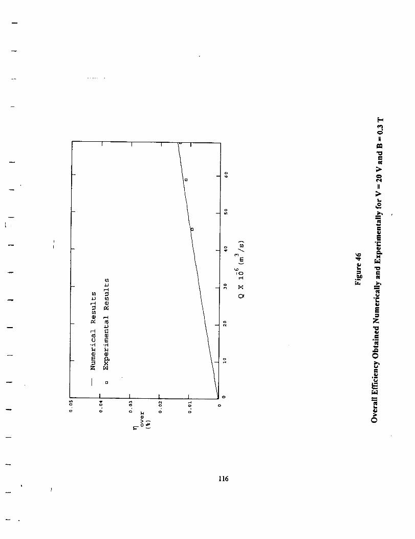
I I i I I

/°

ul

r-t

•I..) _/)r-_ _

"_ "M14 _4(D IlJ

I D

I I I I

®

__o_

o0 0

o

E

_D

iO

C>

m.0

u

01

H

I_

Nm

I;

"I::

M

II

mm

"i::

o_II

mN

I...

116

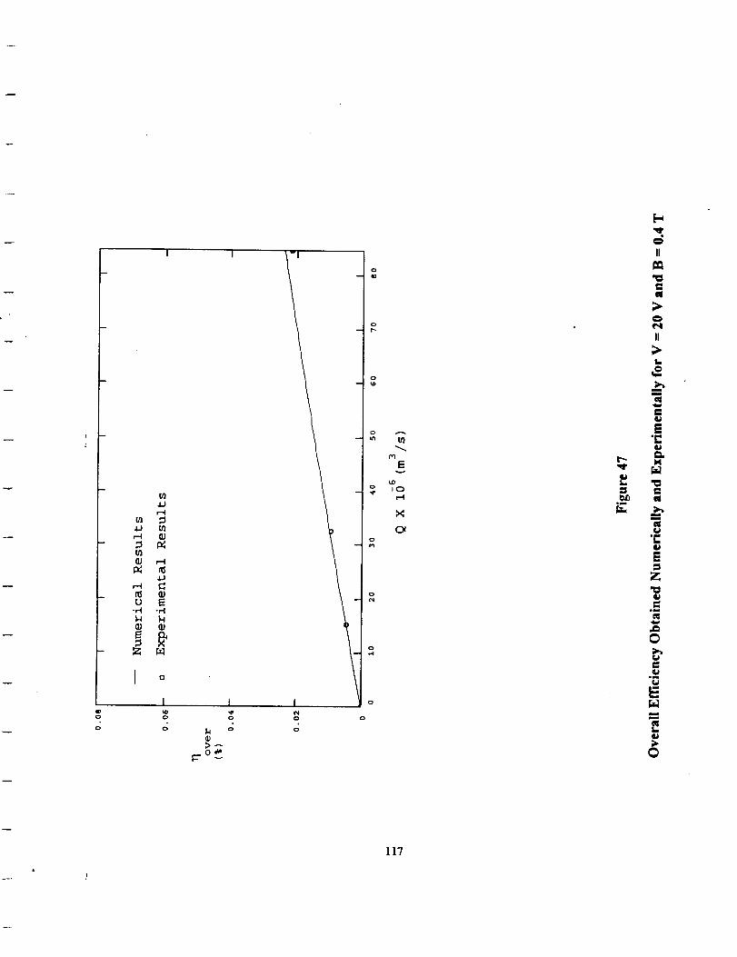
I

u)

U E

E

I 0

I

I t I

o®_A

I_.-o _

o

o o

E

IO

X

L,

om

II

i

0

II

Ii

m

"r

E

0

EN

0

117

APPENDICES

L

118

Appendix A

Computer Prozram

'FINITE DIFFERENCE FOR EHD PUMP

'WRITTEN BY WORANUN WORAMONTRI

CLEAR

SCREEN 0

COLOR 4, 7

CLS

LOCATE 3, 20

PRINT "Finite difference for EHD Conduction Pump"

LOCATE 5, 37

PRINT "By"

LOCATE 7, 30

PRINT "Woranun Woramontri"

'MENU

COLOR I, 7

LOCATE ii, 20

PRINT "i. Find Velocity Profile Only"

LOCATE 13, 20

PRINT "2. Find P-Q Relationship Only"

LOCATE 15, 20

PRINT "3. Find Velocity Profile and P-Q Relationship"

i0 LOCATE 20, 20

119

LCOLOR 6, 7

INPUT "Please select (1-3) "

COLOR i, 7

, menu

SELECT CASE menu

CASE 1

CASE 2

CASE 3

CLS

LOCATE 5, 24

COLOR 3, 8

PRINT ,, VELOCITY PROFILE CALCULATION ,,

CLS

LOCATE 5, 24

COLOR 12, 1

PRINT ,, PRESSURE-FLOW RATE CALCULATION

CLS

COLOR 14, 3

LOCATE 5, 29

PRINT " VELOCITY PROFILE ,,

LOCATE 7, 37

PRINT ,,AND ,,

LOCATE 9, 24

PRINT " PRESSURE-FLOW RATE CALCULATION

CASE ELSE

120,I

GOT0 i0

END SELECT

COLOR I, 7

I,

'INPUT DATA

LOCATE 12, 20

INPUT "Number of Vertical Nodes"; nv

IF nv = 0 THEN nv = ii

LOCATE 13, 20

INPUT "Number of Horizontal Nodes"; nh

IF nh = 0 THEN nh = 41

LOCATE 14, 20

INPUT "Distance Between Nodes"; h

IF h = 0 THEN h = 0.00006392

LOCATE 15, 20

INPUT "Length of the Pump"; length

IF lenth = 0 THEN length = 0.1016

LOCATE 16, 20

INPUT "Magnetic Flux Density"; b

LOCATE 17, 20

INPUT "Voltage apply Across the Electrodes"; volt

SELECT CASE menu

CASE 1

121

LOCATE 18, 20

INPUT "Pressure Rise Across the Pump"; dp

LOCATE 19, 20

INPUT "File to Write Velocity Profile"; vel$

vel$ = vel$ + ".DTA"

OPEN vel$ FOR OUTPUT AS #I

dta = 1

CASE 2

LOCATE 18, 20

INPUT "Maximum Pressure Rise Across the

Pump"; maxdp

LOCATE 19, 20

INPUT "Data Points Required (for P-Q)"; dta

LOCATE 20, 20

INPUT "File to Write Pressure-Flow Rate";

Pq$

pq$ = pq$ + ".DTA"

OPEN pq$ FOR OUTPUT AS #2

CASE 3

LOCATE 18, 20

INPUT "Maximum Pressure Rise Across the

Pump"; maxdp

LOCATE 19, 20

INPUT "Data Points Required (for P-Q)"; dta

122

L_

LOCATE 20, 20

INPUT "File to Write Pressure-Flow Rate";pq$

OPEN pq$ FOR OUTPUT AS #2

LOCATE 21, 20

INPUT "File to Write Velocity Profile"; vel$

CASE ELSE

CLS : PRINT "There is no such a mode!"

END SELECT

'INITIALIZE CONSTANTS

'S .O. R CONSTANTS

w = 1.7

ww = 1 - w

'ELECTROMAGNETIC�FLUIDIC CONSTANTS

sig = 4.44

mu = .000935

E = volt / ((nh - i) * h)

'OPTIMAL S.O.R VALUE

'FLUID CONDUCTIVITY

'FLUID DYNAMIC VISCOSITY

'ELECTRIC FIELD

'FINITE DIFFERENCE CONSTANTS

disv = (nv - I) / i0

dish = (nh - I) / I0

'FOR DISPLAY PURPOSE

'SYSTEM CONSTANTS

123

itr = 1'BEGIN WITH ITERATION = 1

'VELOCITY PROFILE ARRAY

DIM u(nh, nv)

[,

'BOUNDARY CONDIT-IONS

FOR i = 0 TO nh - 1

u (i, 0) = o

u(i, nv - I) = 0

NEXT i

FOR j = 0 TO nv - 1

u(0, j) = 0

u(nh - i, j) = 0

NEXT j

'********** PHASE I STARTS HERE **********

'BEGIN ITERATION

30 'CONTINUE

'PRESSURE CONSTANT

IF menu = I THEN

p = dp / length

ELSE

pincre = maxdp / (length * (dta -

I))

p = pincre * k

124

END IF

kl = (b ^ 2 * sig) / mu 'kl

k2 = (p / mu) - ((sig * E * b) / mu) 'k2

cl = 4 + kl * h * h 'cl

c2 = k2 * h * h 'c2

'FILE NAME FOR VELOCITY PROFILE CASE 3

IF menu = 3 THEN

END IF

decl = INT(k / i0)

dec2 = i0 * ((k / I0)

FOR i = 0 TO 9

NEXT i

- INT(k / i0))

IF decl = i THEN LET decl$ = CHR$(48

+ i)

IF dec2 = i THEN LET dec2$ = CHR$(48

+ i)

yes = vel$ + decl$ + dec2$ + ".DTA"

OPEN ve$ FOR OUTPUT AS #i

CLS

LOCATE 2, I0

COLOR 4, 7

PRINT "Phase I on progress"

COLOR 0, 7

]25

LOCATE 3, i0

PRINT "Pressure Rise ="; p * length

IF menu <> 1 THEN

LOCATE 3, 30

PRINT "( Max ="; maxdp; "

• length; ") "

END IF

LOCATE 4, I0

PRINT "Calculating Velocity Profile"

COLOR 6, 7

LOCATE 22, 10

PRINT "Press <s> to stop the iteration"

COLOR I, 7

DIFF = 1

Step = "., pincre

WHILE INKEY$ <> "s" AND DIFF >= .0000001 AND itr <

300

FOR j = 1 TO nv - 2

FOR i = 1 TO nh - 2

'Check Convergence

IF INT(itr / i0) = itr / i0 AND i = (nh - I) / 2 AND

j = (nv - I) / 2 THEN

DIFF = ABS(uref - u(i, j))

uref = u(i, j)

END IF

UU(i, j) = u(i,j)

126

u(i, j) = 1 / cl * (u(i + I, j) + u(i - I, j) +

u(i, j + i) + u(i, j i) - c2)

u(i, j) = ww * UU + w * u(i, j)

NEXT i

N XT j

LOCATE 6, I0

COLOR 6, 7

PRINT "This is the "; itr; "th Iteration,,

COLOR i, 7

itr = itr + 1

FOR j = 0 TO I0

LOCATE 8 + j, i0

PRINT "value of u("; (nh - i) / 2; ","-, j * disv; ,,)

is equal to"

COLOR 4, 7

LOCATE 8 + j, 45

PRINT USING "##.####### .... ,,., u((nh - i) / 2, j *

disv)

COLOR I, 7

NEXT j

WEND

'PHASE I COMPLETE

BEEP

LOCATE 2, 10

PRINT "Phase I completed ,,

]27

It

IF menu = 2 THEN GOTO 20 'SKIP THIS PROCESS

LOCATE 4, i0

PRINT "

LOCATE 22, i0

PRINT "Writing file to disk

LOCATE 23, i0

PRINT "Please wait..."

'WRITING FILE FOR VELOCITY PROFILE

FOR j = 0 TO nv - 1

FOR i = 0 TO nh - 1

PRINT #i, USING ,,##.#######^AA^,,; u(i, j)

NEXT i

NEXT j

CLOSE #i

'********** PHASE II STARTS HERE **********

20 'CONTINUE

CLS

LOCATE 2, i0

PRINT "Phase II on progress"

LOCATE 4, i0

PRINT "Calculating Volume Flow Rate"

128

sigma = 0

FOR j = 1 TO nv - 2

FOR i = 1 TO nh - 2

sigma = sigma + u(i, j)

NEXT i

NEXT j

q = sigma * h * h

area = h * h * (nh - i) * (nv - i)

vavg = q / area

CLS

COLOR 4, 7

LOCATE 2, 10

PRINT "Phase II completed"

LOCATE 9, 12

COLOR I, 7

PRINT "Volume flow rate equal to

LOCATE II, 12

PRINT "Cross-sectional Area equal to

LOCATE 13, 12

PRINT "Avg. Vel. equal to

IF menu <> 1 THEN

END IF

itr = 1

k = k + 1

"., vavg; "M/S"

length; q

129

1, , ,l, q; MA3/S ''

"; area; "MA2"

PRINT #2, USING ,,##.#######^^^A,,; p

IF k < dta THEN GOTO 30

IF menu = I THEN END

CLOSE #2

END

L

t

130

t

Appendix B

Fluid Properties i

A copper sulfate solution was used as the working fluid for the model verification.

Its concentration was 133.4 g (CuSO4. 5H20) per liter of water at STP conditions. Its

other properties, also at STP, are shown in Table B. 1.

Table B. 1

Properties of Copper Sulfate Solution

Density kg(m--y)

Dynamic Viscosity ( k_a )

m • s

C 2 " SConductivity ( )

kg" m 3

1073

9.35xi0 -4

4 .44

131

• Avvendix C

Wire Size Calculation for the Electromagnet

An analysis was performed to determine the appropriate wire size required for the

electromagnet. The magnetomotive force required to produce the magnetic flux density

of 0.4 T was initially calculated from which the appropriate wire size was determined.

Figure C.1 illustrates the geometry of the electromagnet. Table C. 1 summarizes the

electrical properties of the solid copper wire considered for this application.

The magnetomotive force, expressed in terms of ampere-turns, is determined from:

NI = B A_,,_ Rtot (C.1)

where N is the total number of turns, I is the current, B is the magnetic flux density, Acorc

is the core cross-sectional area and Rtot is the total reluctance of the magnetic circuit.

From the geometry of the electromagnet shown in Figure C.1, Rtot can be

expressed as,

Riot Rl=--+2R 2 +R 32 (c.2)

where:

RI -- Ii

g core/ds

R 2 -- 12

Acor© _Us

132

The values of lengths 11, !2 and 13 are shown in Figure C. 1.

steel core Ps is approximated as:

#, = 250 #o (c.3)

where P-o is the permeability of free space.

According to this analysis, 4206 ampere-turns of the magnetomotive force is

required to produce 0.4 T of magnetic flux density at the air gap.

In order to obtain the required current for each wire size, the number of winding

turns for each wire size (N) was calculated. The approximation of the winding turns can

be determined from:

The permeability of the

N -- Ac°il

A,aro (C.4)

where Acoil is the total cross-sectional area of the coil and Awire is the cross-sectional area

of the wire. The currents required for each wire size were then calculated from:

NI 4206

N N (C.5)

An approximation for the length of the

calculated by:

Looil = C,oll N

where Ccoil is the mean circumference of the coil.

wire used for each case (].,coil) was

(C.6)

The total resistance of the coil (Rcoil)

was then calculated from the total length and the wire property given in Table C. 1. From

the current and resistance of each wire size, the required voltage is calculated from:

V.,,il = I**il r (C.7)

Figure C.2 shows the required voltages for various wire sizes. The required

currents for various wire sizes are shown in Figure C.3. From Figures C.2 and C.3, #18

AWG was considered to be the appropriate wire size for this particular application.

133

NE

IW _D

_ U <E£

CJ

<E

i

I

II '

E E E IW

eO U")o (:7_('Do I",,o•" C_ CU r--cD"_N_dddmII II II I1_

0

0

0

0I--

ej

_Jlai_.

_o.u

la

01 .

cata

N

laJ_

s.=.o

qa

o

134

L

Jm

I,,,

m_o

r_"O

m

I=

O

,nl

,',,.0L

i:::

,m0• U

o_

0

v

0

rj

_o_o_ .......... _ $_...... 0 _ 0 _ _ _ _ _ _

r,D

r..O

-.-I

135

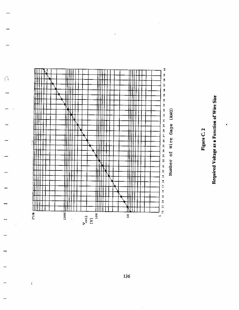
0

tn

0

@

@.m

tli

.m

@

,m

136

om

o

oom

om

t...t...

t...o_

137

At3Dendix D

,Calculated and Measured Magnetic Flux Density

l

0.6

B(T)

0.4

0.2

1 _ 1 I J I I I I I I

L0.8/7

Predicted Value

o Measured Value _ -

i ° iD 0

0 D 0 0

0 "t/ J I I I I I I I I0 1 2 3 4 5 6 _ 8 9 lO

Icoii (Ampere)

Figure D. 1

Comparison of the Calculated and Measured Magnetic Flux Density

138

A_pendix E

=Calibration Curve for the Rotameter

In order to obtain accurate readings, the rotameter used in the experiments was

calibrated for the test fluid as shown in Figure E. I.

300I i I I I i I I I

250

200

QXl O" 6

m 3 /8

150

ioo

5o

0 0.5 1I I I I I I I

1.5 2 2.5 3 3.5 4 4.5

Rotameter Reading (gpm)

Figure E. 1

Calibration Curve for the Rotameter

139

absorfrion heat pump for space applications final report …

Documents