absolute stability of wavetrains can explain ...jas/paperpdfs/smithrademachersherratt2009.pdf ·...

Copyright © by SIAM. Unauthorized reproduction of this article is prohibited.

SIAM J. APPLIED DYNAMICAL SYSTEMS c© 2009 Society for Industrial and Applied MathematicsVol. 8, No. 3, pp. 1136–1159

Absolute Stability of Wavetrains Can Explain Spatiotemporal Dynamics inReaction-Diffusion Systems of Lambda-Omega Type∗

Matthew J. Smith†, Jens D. M. Rademacher‡, and Jonathan A. Sherratt§

Abstract. The lambda-omega class of reaction-diffusion equations has received considerable attention becausethey are more amenable to mathematical investigation than other oscillatory reaction-diffusion sys-tems and include the normal form of any reaction-diffusion system with scalar diffusion close to astandard supercritical Hopf bifurcation. Despite this, detailed studies of the dynamics predictedby numerical simulations have mostly been restricted to regions of parameter space in which stablewavetrains (periodic traveling waves) are selected by the initial or boundary conditions; we use theterm “stability” to denote spectral stability on the real line. Here we consider the emergent spa-tiotemporal dynamics on large bounded domains, with Dirichlet conditions at one boundary andNeumann conditions at the other. Previous studies have established a parameter threshold belowwhich stable wavetrains are generated by the Dirichlet boundary condition. We use numerical con-tinuation techniques to analyze the spectral stability of wavetrain solutions, and we identify a secondstability threshold, above which the selected wavetrain is absolutely unstable. In addition, we provethat the onset of absolute stability always occurs through a complex conjugate pair of branch pointsin the absolute spectrum, which greatly simplifies the detection of this threshold. In the parame-ter region in which the spectra of the selected waves indicate instability but absolute stability, ournumerical simulations predict so-called “source-sink” dynamics: bands of visibly regular periodictraveling waves that are separated by localized defects. Beyond the absolute stability threshold oursimulations predict irregular spatiotemporal behavior.

Key words. AUTO, parabolic partial differential equations, complex Ginzburg–Landau equation, absolutespectrum, plane waves

AMS subject classifications. 35K57, 35B35, 35P05

DOI. 10.1137/090747865

1. Introduction. A wide range of physical and natural systems exhibit dynamics thatare the result of local interactions between their components and of diffusive dispersal. Thedynamics of such systems are often studied mathematically using reaction-diffusion equations.An important subset of such equations are those in which the local interactions between thecomponents of the system lead to cyclic dynamics, so that the reaction kinetics have a stablelimit cycle. Such oscillatory reaction-diffusion systems have been used effectively as models

∗Received by the editors January 26, 2009; accepted for publication (in revised form) by D. Barkley June 19,2009; published electronically August 26, 2009.

http://www.siam.org/journals/siads/8-3/74786.html†Computational Ecology and Environmental Science Group, Microsoft Research, Cambridge CB3 0FB, UK

([email protected]). This author was supported in part by an Environmental Mathematics and Statis-tics (EMS) studentship from the Natural Environment Research Council (NERC) and the Engineering and PhysicalSciences Research Council (EPSRC), and by Microsoft Research.

‡Centre for Mathematics and Computer Science (CWI), Kruislaan 413, 1098 SJ Amsterdam, The Netherlands([email protected]). The work of this author was supported by the NWO cluster NDNS+.

§Department of Mathematics and Maxwell Institute for Mathematical Sciences, Heriot-Watt University, EdinburghEH14 4AS, UK ([email protected]). This author was supported in part by a Leverhulme Trust Research Fellowship.

1136

http://www.siam.org/journals/siads/8-3/74786.html

mailto:[email protected]




ABSOLUTE STABILITY OF WAVETRAINS 1137

for many phenomena (see [26] for a review). Oscillatory reaction-diffusion equations cangenerate a wide range of spatiotemporal dynamics, including target patterns, spiral and scrollwaves, localized breathers, and spatiotemporal irregularities (see [14, 58, 35] for reviews ofthese phenomena). From an applied perspective, studies of such equations center aroundunderstanding the predicted dynamics and interpreting their implications for the physical,chemical, or biological systems concerned. A key issue for this is the stability of spatiotemporalsolutions. The building block for all such solutions is one-dimensional wavetrains, and theirspectral stability on unbounded and large bounded domains (see [35] for a review) is the focusof this paper.

Over the last decade, significant new mathematical insights have been gained into thestability of solutions of reaction-diffusion equations. In particular, it is now clear that theunderstanding of spatiotemporal behavior is helped by considering various different types of(in)stability and by distinguishing stability on the real line and on large periodic domainsfrom stability on large bounded domains with separated boundary conditions (see [38] for amore detailed discussion than that given here). These distinctions are made on the level of thespectrum of the equations when linearized about a solution, and we call a solution (spectrally)stable if, on the whole real line, all modes (except the neutral translation mode) decay on thereal line. Classifications of instability distinguish between different spatiotemporal dynamicsof the growing perturbations. On the real line, for “convectively unstable” solutions, pertur-bations grow while traveling away from the site of the perturbation but decay at the site ofperturbation itself; by contrast, for “absolutely unstable” solutions, perturbations grow at allpoints in space, including the site of perturbation. The most widespread application of thesedifferent types of stability has been to problems in fluid dynamics (reviewed by [21, 13]) andspiral wave break-up (e.g., [2, 39, 59]).

In this paper we study the stability of wavetrain solutions for a particular system ofoscillatory reaction-diffusion equations in one space dimension:

ut = uxx + (1 − r2)u − (ω0 − ω1r2)v,(1a)

vt = vxx + (1 − r2)v + (ω0 − ω1r2)u.(1b)

Here u and v are the variables of the system, subscripts t and x denote partial derivatives withrespect to time and space, r = (u2 + v2)1/2, and ω0 and ω1 are constants. For mathematicalsimplicity, we will assume that ω0 > ω1 > 0, which ensures that ω0−ω1r

2 �= 0 for any r ∈ [0, 1],which is an invariant region [6]. Equations (1) are a special case of the complex Ginzburg–Landau equation (see [1] for a review) and have a wide relevance for oscillatory systems, beingthe normal form of an oscillatory reaction-diffusion system with equal diffusivities, when thekinetics are close to a standard supercritical Hopf bifurcation. They belong to the “lambda-omega” class of reaction-diffusion equations, introduced by Kopell and Howard [22]. Theseauthors showed that such equations are much more amenable to mathematical analysis thanmost oscillatory reaction-diffusion equations. In particular, they showed that (1) has a one-parameter family of wavetrain solutions, of the form

u = R cos[θ0 ± x

√1 − R2 +

(ω0 − ω1R

2)t],(2a)

v = R sin[θ0 ± x

√1 − R2 +

(ω0 − ω1R

2)t],(2b)


1138 MATTHEW SMITH, JENS RADEMACHER, AND JONATHAN SHERRATT

where amplitude R (0 ≤ R ≤ 1) parameterizes the family and θ0 is an arbitrary constant.Moreover, they calculated an exact condition for the stability of the waves, namely,

(3) R > ress ={

2 + 2ω21

3 + 2ω21

}1/2

.

Simulation-based studies of oscillatory reaction-diffusion equations have shown that wave-trains often arise when initial or boundary conditions are inconsistent with spatially uniformoscillations. Further, the relative simplicity of (1) has enabled such “wave selection” prob-lems to be studied analytically [44, 42, 18, 41, 50]. One important conclusion in these papersis that for some parameters, the selected wave is in fact unstable. In such cases, numeri-cal simulations often show spatiotemporal irregularity as the long-term behavior. However,no detailed characterization of this behavior has previously been undertaken. Our objectivein this paper is to obtain a deeper understanding of the spatiotemporal behavior arising insimulations of (1) in the regions of parameter space in which unstable waves are selected.We will principally focus on wave selection in (1) by Dirichlet boundary conditions at oneedge of a large bounded domain. We have used this wave selection scenario in the past toinvestigate the occurrence of wavetrains in ecological systems, where the Dirichlet boundarycondition is analogous to an inhospitable environment at the edge of a habitat (see [47] fora recent review), and it has also been used to investigate the generation of traveling wavesin oscillatory chemical reactions [3]. Our study here is intended to benefit future research inthese areas by illustrating how the variety of dynamics observed in numerical simulations canbe explained by analyzing the spectral stability of the selected wavetrains. In the discussion(section 6) we also briefly consider the generation of wavetrains when the spatially uniform(unstable) steady state u = v = 0 receives a small localized perturbation. This “invasion” sce-nario has been studied extensively in the context of physical, chemical, and ecological systems[31, 57, 19, 47, 48].

In our study here we will determine which of the unstable waves are absolutely unstable,using the numerical continuation approach developed by [33]. We will show that this spectralinformation alone gives valuable insights into the spatiotemporal dynamics resulting from so-lutions of the partial differential equations. We begin (section 2) by describing the results ofnumerical simulations of wavetrain generation. We then (section 3) outline the general theoryof absolute stability and prove a new result on the relationship between the original “pinch-ing condition” for absolute stability [12] and the more recent approach using the absolutespectrum [38]. We also prove that for the particular case of the lambda-omega system (1),absolute stability is determined by specific points in the absolute spectrum, known as “branchpoints” [38]. In section 4 we develop a systematic approach for the numerical calculationof the absolute spectrum. This provides an efficient way of identifying parameter thresholdsfor absolute stability, and the supplementary online material [49] contains a detailed tutorialguide and sample code to facilitate the implementation and adaptation of this approach byothers. In section 5 we discuss details of the “source-sink” dynamics that we observe for pa-rameters such that the boundary condition selects a convectively unstable wavetrain. Finally,in section 6 we draw conclusions and briefly discuss the dynamics that arise from wavetraingeneration behind invasion fronts.



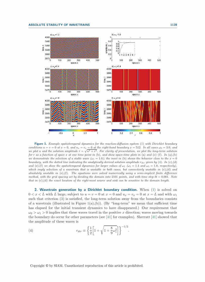
Figure 1. Example spatiotemporal dynamics for the reaction-diffusion system (1) with Dirichlet boundaryconditions u = v = 0 at x = 0, and ux = vx = 0 at the right-hand boundary x = 512. In all cases ω0 = 3.0, andwe plot u and the solution amplitude r =

√u2 + v2. For clarity of presentation, we plot the long-term solution

for r as a function of space x at one time point in (b), and show space-time plots in (a) and (c)–(f). In (a),(b)we demonstrate the selection of a stable wave (ω1 = 1.0); the inset in (b) shows the behavior close to the x = 0boundary, with the dotted line indicating the analytically derived solution amplitude rdir given by (4). In (c),(d)and (e),(f) we show the spatiotemporal dynamics for larger values of ω1 (ω1 = 1.4 and ω1 = 1.8, respectively),which imply selection of a wavetrain that is unstable in both cases, but convectively unstable in (c),(d) andabsolutely unstable in (e),(f). The equations were solved numerically using a semi-implicit finite differencemethod, with the grid spacing set by dividing the domain into 2101 points, and with time step δt = 0.001. Notethat in (c),(d) the exact location of the right-most source and sink can be sensitive to the domain length.

2. Wavetrain generation by a Dirichlet boundary condition. When (1) is solved on0 < x < L with L large, subject to u = v = 0 at x = 0 and ux = vx = 0 at x = L and with ω1

such that criterion (3) is satisfied, the long-term solution away from the boundaries consistsof a wavetrain (illustrated in Figure 1(a),(b)). (By “long-term” we mean that sufficient timehas elapsed for the initial transient dynamics to have disappeared.) Our requirement thatω0 > ω1 > 0 implies that these waves travel in the positive x direction; waves moving towardsthe boundary do occur for other parameters (see [41] for examples). Sherratt [41] showed thatthe amplitude of these waves is

(4) rdir ≡{

12

[1 +

√1 +

89ω2

1

]}−1/2

.



Close to the x = 0 boundary, the solution amplitude drops from this value to zero; specificallythe long-term solution away from x = L is (see [41])

(5) r = rdir tanh(x/

√2)

.

In the language of the complex Ginzburg–Landau equation, this solution form is a stationaryNozaki–Bekki hole [27, 29, 4]. One simple application of (4) is to assess the accuracy ofnumerical solutions, and throughout this study we will use a numerical discretization thatgives a wave amplitude differing (in stable cases) from (4) by about 0.1%. Note that the spaceand (especially) time step required for this depend strongly on ω0 (see Appendix C of [50] fordetails).

The criterion (3) of Kopell and Howard [22] implies that the wavetrain with amplituderdir is stable (on the real line or in the limit of large L for periodic boundary conditions) if andonly if ω1 < 1.110468. A key focus of our work is to calculate the corresponding condition forabsolute stability, which we will show to be ω1 < 1.576465. In Figure 1(c)–(f), we show typicalnumerical simulations for one value of ω1 below this threshold (but above 1.110468) and oneabove it. Corresponding movies, which are very helpful in understanding the dynamics, canbe viewed at http://research.microsoft.com/en-us/projects/loptw/, or can be generated byrunning the “Lambda-Omega Equations Solver” (which is freely available from the same Webpage).

When a convectively unstable wave is selected, the long-term behavior consists of bands ofperiodic waves traveling in opposite directions and separated by apparently stationary defects(Figure 1(c),(d)). We will discuss this solution form in detail in section 5, showing that thedefects do in fact move over very long time scales. In contrast, for ω1 > 1.576465, so thatan absolutely unstable wave is selected, the solution is irregular in space and time (Figure1(e),(f)).

3. Absolute stability of wavetrains. To calculate spectral stability of a wavetrain solutionof a reaction-diffusion system we linearize the equations about this solution. In general,the coefficients of the resulting linear equations are periodic functions of the traveling wavecoordinate. However, lambda-omega equations such as (1) can be converted into amplitude-phase form, and linearizing about a wavetrain then gives a system with constant coefficients.From the viewpoint of numerical continuation methods for determining stability, this is amajor simplification (see [33] for a detailed discussion). Substituting u = r cos θ and v = r sin θinto (1) gives

rt = rxx + r(1 − r2) − rθ2x,(6a)

θt = θxx + (ω0 − ω1r2) +

2rxθx

r,(6b)

with the wavetrain solution (2) being r = R and θ = (ω0 − ω1R2)t ± x

√1 − R2 (0 ≤ R ≤ 1).

To leading order, small perturbations r(x, t) and θ(x, t) of this solution satisfy

rt = rxx − 2R2r − 2Rθx

√1 − R2,(7a)

θt = θxx − 2ω1Rr +2rx

√1 − R2

R.(7b)

http://research.microsoft.com/en-us/projects/loptw/



In the standard way, we look for solutions of the form (r, θ) = (r, θ)eλt+νx, where r and θ areconstants, giving

λr = ν2r − 2R2r − 2νRθ√

1 − R2,(8a)

λθ = ν2θ − 2ω1Rr +2νr

√1 − R2

R.(8b)

This implies the dispersion relation

0 = A(λ, ν) ≡ λ2 − 2λ(ν2 − R2) + ν2(ν2 + 4 − 6R2) − 4ω1νR2√

1 − R2(9)

= ν4 + 2ν2(2 − 3R2 − λ) − 4ω1νR2√

1 − R2 + λ(λ + 2R2)

as the condition for nontrivial solutions. Note that A(0, 0) = 0 for all R, reflecting the neutralstability of the waves to translation. Note also there is no cubic term for ν in this equation,which is a simplifying feature for the analysis below.

For stability (on the whole real line) we must consider values of λ satisfying A(λ, ν) = 0,with ν pure imaginary; the set of such λ’s is known as the “essential spectrum,” denoted byΣess. The condition for stability is that Re(λ) < 0 for all λ in the essential spectrum, exceptλ = 0. Kopell and Howard [22] showed that this condition reduces to R > ress (defined in (3)).

To address the distinction between absolute and convective instability, we introduce theso-called absolute spectrum. To describe this, we return to the dispersion relation A(λ, ν) = 0.For each λ, this has four roots for ν, which we denote by νi(λ) (i = 1, 2, 3, 4), labeled so that

Re(ν1) ≥ Re(ν2) ≥ Re(ν3) ≥ Re(ν4).

We refer to the label i of νi(λ) in this ordering as the index of the root. The “generalizedabsolute spectrum” is the set of λ such that Re(νi) = Re(νi+1) for some i = 1, 2, or 3. The“absolute spectrum” Σabs is a subset of the generalized absolute spectrum, and for a systemof two coupled reaction-diffusion equations it is the set of λ for which Re(ν2) = Re(ν3) (fordetails, see [38] and Corollary 3 below). The complement of the absolute spectrum in thegeneralized absolute spectrum, where the index of the repeated roots for ν in our equationsis either 1 or 3, has no direct relevance for the stability of selected wavetrains in numericalsimulations or for the spectrum of the operator. We refer to the proofs in [38] for furtherdetails on this part of the generalized absolute spectrum. We calculate the full generalizedabsolute spectrum in this paper because it allows us to systematically compute the absolutespectrum.

Despite its name, the absolute spectrum is not a spectrum in the sense of solutions to aneigenvalue problem. However, its relevance for the spectrum on large bounded domains is asfollows. Consider the spectrum ΣL of the linearization of (1) in a (near) wavetrain solutionposed on the domain (−L,L). Then for generic separated linear boundary conditions, Σabs

is the set of accumulation points of ΣL as L → ∞. In particular, instability of the abso-lute spectrum implies an instability on all sufficiently large domains. Note that for periodicboundary conditions, the set of accumulation points of ΣL as L → ∞ is the essential spectrum.Sandstede and Scheel [38] give a full discussion of these ideas.



Im(λ)

Gabs

Re(λ)

Gess

Re(λ)

Im(λ)

Λ

λ0

(a) (b)

Figure 2. (a) A fictional set Gabs ⊂ C (shaded region). The solid curves are the absolute spectrum Σabs,the bullets are branch points in ∂Gabs, and the square a branch point in Gabs \∂Gabs. (b) A fictional set Gess ⊂ C

(shaded region) consistent with Gabs in (a). The thick solid curves are the essential spectrum Σess, the thinsolid lines Σabs, and the bullets and square are as in (a). We plot in addition a possible point λ0 and curve Λ(dotted) for the proof of Lemma 1.

The notions of absolute and convective instabilities were first developed for the wholereal line [12], and in this case only simultaneous roots of A and ∂νA, referred to as branchpoints, are meaningful; trivially, these are contained in the generalized absolute spectrum. Asmentioned, an absolute instability means that perturbations lead to pointwise growth, andthis occurs when a branch point of the dispersion relation, with positive real part, satisfiesthe so-called pinching condition [12, 11, 9, 8], which is explained below.

We now prove a lemma that makes a connection between the pinching condition and theabsolute spectrum; the result may be well known, but we are not aware of a reference. Wedo not attempt to explore the connection in full generality here. Rather, we focus on thelambda-omega system (1), for which the combination of the lemma and Corollary 3 belowimplies that absolute stability is determined by branch points in the absolute spectrum thatsatisfy the pinching condition. Let (λ∗, ν∗) be a branch point, with ν±(λ) continuous curvesof solutions to A = 0 with ν±(λ∗) = ν∗. The “pinching” or “collision” condition is satisfied at(λ∗, ν∗) if, for suitable choices of ν±, it holds that sgn(Re ν±(λ)) = ±1 as Re(λ) → +∞. Thisis satisfied if the sign condition holds for values of λ with sufficiently large real part along anycurve of λ values emanating from λ∗. In fact, the real parts of all ν are unbounded, as the realpart of λ tends to infinity (see, for example, Lemma 3.3 in [32]). As defined above, we referto solutions with unstable essential spectrum, but stable absolute spectrum, as convectivelyunstable; we use the term “absolutely unstable” if the absolute spectrum is unstable.

In preparation, denote by Gabs the connected component of C \ Σabs that contains anunbounded part of the real axis, and by Gess the connected component of C\Σess that containsan unbounded part of the real axis (illustrated schematically in Figure 2); these sets are welldefined [38, 39].

Lemma 1.1. All branch points (λ∗, ν∗) for which λ∗ lies on the boundary ∂Gabs satisfy the pinching



condition.2. At all branch points (λ∗, ν∗) satisfying the pinching condition, λ∗ lies in C \ Gabs, so

that Re(λ∗) ≤ maxRe Σabs.Proof. It is well known that for a system of two coupled reaction-diffusion equations such

as (1) the Morse index i(λ) := #{ν(λ) : Re(ν(λ)) ≥ 0} of any λ ∈ Gess is i(λ) = 2, and thatGess∩Σabs = ∅ (see, for example, [37]). The idea underlying our proof is to look for changes inthe ordering of the real parts of ν(λ) along a curve Λ in the complex λ plane connecting thebranch point λ∗ to a point λ0 ∈ Gess; see Figure 2(b) for an illustration. From the definitionof Gess, the Morse index i(λ0) is the same for all λ0 in this region. In the following we labelcurves with indices denoting the ordering at λ∗: we denote by νj(λ) the continuation of νj(λ∗)along Λ; i.e., νj is continuous and νj(λ∗) = νj(λ∗). Note that since λ∗ ∈ Σabs and is a branchpoint, ν2(λ∗) = ν3(λ∗).

Item 1. Since λ∗ ∈ ∂Gabs we can choose Λ so that Λ∩Σabs = {λ∗}. The pinching conditionfails if and only if sgn(Re(ν2(λ0))) = sgn(Re(ν3(λ0))), and we suppose this to be the case.Since i(λ0) = 2 it follows that either Re(ν1(λ)) or Re(ν4(λ)) has to change sign along Λ, andwe next show that this implies the contradiction Λ ∩ Σabs �= {λ∗}.

Suppose that sgn(Re(ν2,3(λ0))) = sgn(Re(ν∗)) = −1. Since i(λ0) = 2 and ν∗ = ν2(λ∗), itfollows that Re(ν1(λ0)) > 0. Therefore the νj’s reorder along Λ in a way that gives ν1(λ0) =νj(λ0) for j = 2 or j = 3. Hence there are points λ� ∈ Λ (� = 2, 3) different from λ∗ at whichRe(ν1(λ�)) = Re(ν�). Since the ordering changes in increments of one (or simultaneously), oneof these points lies in Σabs, which contradicts Λ ∩ Σabs = {λ∗}. Hence, sgn(Re(ν2,3(λ0))) =sgn(Re(ν∗)) = −1 cannot hold true.

The same argument, now applied to ν3(λ), shows that sgn(Re(ν2,3(λ0))) = sgn(Re(ν∗)) =+1 also contradicts the assumption. In the cases sgn(Re(ν2,3(λ0))) = − sgn(Re(ν∗)) the sameargument applies again, with ν1(λ) if sgn(Re(ν∗)) = +1 and ν3(λ) otherwise.

In conclusion, Re(ν2,3(λ0)) must have opposite signs, which is the pinching condition.Note that λ0 can be chosen so that Re(ν2,3(λ0)) �= 0.

Item 2. Note that λ∗ /∈ Gess since all points in Gess have the same Morse index, whereasthe pinching condition requires a change. We choose a curve Λ connecting λ∗ to an arbitrarypoint λ0 ∈ Gess and will show that Λ ∩ Σabs �= ∅.

We assume the nontrivial case λ∗ /∈ Σabs so that ν∗ = ν�(λ∗) = ν�+1(λ∗) for � = 1 or � = 3.The pinching condition implies Re(ν�(λ0)) < 0 < Re(ν�+1(λ0)) so that either Re(ν�(λ)) orRe(ν�+1(λ)) changes sign along Λ. Since i(λ0) = 2 another sign change must also occur; i.e.,sgn(Re(νk(λ∗))) �= sgn(Re(νk(λ0))) for either k ≡ � + 2 mod 4 or k ≡ � + 3 mod 4. The realparts of the sign-changing solutions must be the same at least once along Λ. As in item 1, ifthere is one crossing, then there is (also) one in Σabs.

3.1. The most unstable points of the absolute spectrum. The dynamics after the onsetof instability of the absolute spectrum depend on the way in which it becomes unstable.Concerning the distinction between the absolute spectrum and the pinching condition, thequestion is whether the absolute spectrum becomes unstable via a branch point. If not, onehas a so-called remnant instability. In such a case, all linear modes decay in a stationaryframe of reference, but there are unstable modes that grow while traveling to either the leftor the right, enabling a perturbation to grow at its original site via repeated reflections off



the boundaries. We are aware of only one example in which this has been demonstratednumerically (see Figure 10 of [33]). On the other hand, there do not seem to be any rigorousresults showing that the onset of absolute instability occurs via branch points, except intrivial cases. The main difficulty lies in the algebraic complications that arise even for rathersimple dispersion relations. In the following we overcome these difficulties for a certain classof dispersion relations and deduce that the most unstable points in the absolute spectrum forA are branch points. Specifically, we consider a generalization of A given by d : C

2 → C ofthe form

(10) d(λ, ν) = λ2 − 2λ(ν2 − A) + ν4 + Bν2 + Cν

with constants A,B,C ∈ R. The roots λ(ν) of d(λ, ν) = 0 come in the two functions

λ± = ν2 − A ±√

−ν2(2A + B) − Cν + A2.

Theorem 2. If the absolute spectrum Σabs of d(λ, ν) as in (10) with 2A + B > 0 containsa branch point (λ∗, ν∗), where Im(λ∗) �= 0, then the following hold:

1. λ∗ is one of the two unique complex conjugate points that have maximal real part withinΣabs.

2. λ∗ ∈ ∂Gabs, and (λ∗, ν∗) satisfies the pinching condition.3. If additionally C �= 0, then a branch point at the origin cannot lie in the absolute

spectrum but instead has to be in the generalized absolute spectrum with index 1 or 3.Before proving this result, we point out its significance for our purposes.Corollary 3. If the absolute spectrum Σabs of a wavetrain (2) of the lambda-omega sys-

tem (1) for 0 < R < 1 and ω1 > 0 contains a branch point (λ∗, ν∗) with Im(λ∗) �= 0, then λ∗is one of the two unique complex conjugate points that have maximal real part within Σabs.Such a branch point lies in ∂Gabs and satisfies the pinching condition. Moreover, a branchpoint at the origin cannot lie in the absolute spectrum.

Proof. For the dispersion relation of wavetrains in the lambda-omega system (1) we haveA = R2 > 0, B = 4−6R2 so that 2A+B = 4(1−R2) > 0, and C = −4ω1R

2√

1 − R2 < 0.The proof of Theorem 2 is based on the following observation.Lemma 4. For any fixed η ∈ R the real parts of λ±(η + ik) are even functions of k, and

the imaginary parts are odd functions. If 2A + B > 0, then the following hold:1. Re(λ−(η +ik))+Re(λ+(η +ik)) and Re(λ−(η +ik))−Re(λ+(η +ik)) are both strictly

decreasing in k ≥ 0.2. For k > 0 it holds that Re(λ−(η+ik)) is strictly decreasing in k, and that Re(λ+(η+ik))

either is strictly decreasing or is strictly increasing on 0 < k < k∗ and strictly decreas-ing on k > k∗, for some k∗ > 0.

Proof. Since the coefficients of d are real, the real and imaginary parts are respectivelyeven and odd functions of k. To facilitate a more detailed study, we write D = 2A + B,z = −ν2D − Cν + A2, and ν = η + ik, giving

L±(k) := Re(λ±(η + ik)) = η2 − k2 − A ±√

|z| + Re(z)2

.



We readily compute

Re(z) = Dk2 − Dη2 − ηC + A2,

Im(z) = −(2ηD + C)k,

and with F = 2η2D2 + 2ηDC + 2DA2 + C2, G = −Dη2 − ηC + A2, we obtain

(11) |z|2 = Re(z)2 + Im(z)2 = D2k4 + Fk2 + G2.

Item 1. F = 2(ηD + C/2)2 + 2DA2 + C2/2 ≥ 0. Hence, for all η we have that |z|2 isan even function of k and monotone increasing in k ≥ 0, so that |z| has the same properties.Since Re(z) also has these properties, so does |z| + Re(z) ≥ 0. Finally, since |z| + Re(z) ≥ 0,√

|z| + Re(z) also has these properties.Item 2. It follows that Re(λ−(η+ik)) is the sum of two even functions of k that are mono-

tone decreasing in k ≥ 0, and therefore it has these properties itself. However, Re(λ+(η +ik))is the sum of an increasing and a decreasing function, and therefore it requires more carefulinvestigation. Writing K = k2,

(12)∂

∂kL+(k) = 2k

(−1 +

12√

2∂|z|/∂K + ∂ Re(z)/∂K√

|z| + Re(z)

).

Differentiating again shows that if ∂L+(k)/∂k = 0 at k = k∗ > 0, then

∂2

∂k2L+(k)

∣∣∣∣k=k∗

=k√

2(|z| + Re(z))

[∂2|z|∂K2

− 4]

,

and differentiation of (11) shows that

∂2|z|∂K2

=4D2G2 − F 2

4(D4K2 + FK + G2)3/2.

Moreover, 4D2G2 − F 2 = −(2Dη + C)2(4DA2 + C2) ≤ 0. Therefore at any point k∗ > 0at which ∂L+/∂k = 0, ∂2L+/∂k2 is strictly negative. Finally, we note that L+ → −∞ ask → ∞. Therefore L+(k) must have one of the two forms given in item 2.

Proof of Theorem 2. In the following we use the notation of the proof of Lemma 4.Item 1. We begin by applying Lemma 4 with η = Re(ν∗); due to complex conjugation sym-

metry, we can assume without loss of generality that k ≥ 0. Since the branch point is a doubleroot of d with respect to ν, either λ∗ = λ+(ν∗) and ∂λ+/∂ν(ν∗) = 0 (⇒ ∂λ+/∂k(ν∗) = 0) orλ∗ = λ−(ν∗) and ∂λ−/∂ν(ν∗) = 0 (⇒ ∂λ−/∂k(ν∗) = 0). Referring to item 2 of Lemma 4, theonly case that is consistent with this is λ∗ = λ+(ν∗), with λ∗ being nonmonotonic in k, andwith Im(ν∗) = k∗. Since L− − L+ is negative at k = 0 and decays monotonically for k ≥ 0(item 1 of Lemma 4), we have that Re(λ∗) > max{L−(k) : k ∈ R}.

In conclusion, the branch point lies at the maximal real part of the roots of d(λ, η + ik)(k ∈ R). We now note that these roots define the essential spectrum in an exponentiallyweighted space with weight η. Lemma 3.3, Lemma 4.1, and Remark 1 of [32] together showthat for a wavetrain solution of any reaction-diffusion system in one space dimension, the most



unstable point of a weighted essential spectrum is at least as unstable as the most unstablepoint of the absolute spectrum. Therefore in the present case, the weighted essential spectrumand the absolute spectrum must coincide at (λ∗, ν∗), which is the most unstable point of eachspectrum.

Item 2. λ∗ ∈ ∂Gabs follows immediately from the proof of item 1. Lemma 1 then impliesthat the branch point satisfies the pinching condition.

Item 3. If the origin is a branch point, then

d(0, ν) = ν(ν3 + Bν + C) = 0,

whose solutions are ν = 0 and the three roots of a cubic polynomial. Since this cubic doesnot have a quadratic term, the sum of its roots vanishes. Therefore if C �= 0, so that noneof these three roots is zero, the roots must be ν0, ν0, and −2ν0 for some ν0 �= 0. Therefore abranch point must have index equal to either 1 (ν0 > 0) or 3 (ν0 < 0): its index cannot be 2,and thus it cannot be part of the absolute spectrum.

4. Numerical calculation of the absolute spectrum.

4.1. Numerical methodology. Rademacher, Sandstede, and Scheel [33] give a detailedaccount of the use of numerical continuation to calculate the absolute spectrum; here wegive a summary for the specific case of the lambda-omega equations (1), with further detailsprovided in the supplementary online material [49]. Alternative approaches to the numericalcalculation of absolute stability (on the real line) are given in [11, 10, 7, 54, 52, 51, 53]. Forany given λ, (8) can be written in matrix form as

D(λ, νk)Uk = 0,(13a)

where D(λ, ν) = Idν2 + Cν + F − λ, Uk =(

rk

θk

),(13b)

C =(

0 −2R√

1 − R2

2√

1 − R2/R 0

), F =

(−2R2 0−2ω1R 0

),(13c)

and Id is the 2 × 2 identity matrix. Here ν1, . . . , ν4 are the four roots of the dispersionrelation (9). Taking real and imaginary parts of (13) gives 16 equations to be solved simul-taneously. Following [33], we perform numerical continuations of solutions of these equationsusing the software package auto [16, 15, 17]. Specifically, we continue in λ from known solu-tion values and monitor the resulting changes in νk. We ensure that the continuations remainon the generalized absolute spectrum by adding the constraint that two of the values of νk

must have the same real part. Thus, instead of representing the real parts of the two ν valuesseparately, we use a single auto parameter for their common real part.

Starting solutions are necessary to begin the continuations. To obtain these we utilizeCorollary 3 and the general finding of [33] that for constant coefficient problems all curves ofthe generalized absolute spectrum emanate from branch points, with the absolute spectrumbeing a connected subset.

Concerning branch points of A, note that ∂νA = 0 means that

(14) λ = ν2 + 2 − 3R2 − ω1R2√

1 − R2

ν.



To calculate the position of the branch points, we first substitute (14) into the dispersionrelation (9). This gives a fourth order polynomial in ν (which we omit for brevity), zeros ofwhich give four ν values that are double roots of A.

We then calculate the four λ values associated with these double roots by substituting theν values back into (14). (In the supplementary online material [49] we give MATLAB [25]code that calculates these values numerically.) We can also substitute the λ values associatedwith each branch point into (9) and solve for ν to give the other two ν values at any givenbranch point. This allows us to classify the nature of the branch points in terms of the indexof the repeated root for ν.

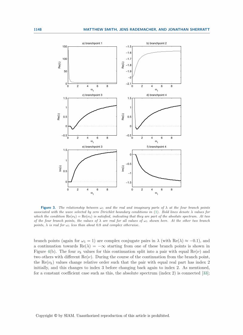
This procedure reveals that for wavetrain solutions of the lambda-omega equations (1),the branch points are either four real λ values or two real λ’s plus a complex conjugate pair.Note that Theorem 2 excludes the possibility of two complex conjugate pairs of branch points.Figure 3 shows these λ’s for the wavetrain selected by the zero Dirichlet boundary condition,as a function of ω1. As ω1 is increased from zero there are initially four real λ values at thebranch points, and at ω1 ≈ 0.8 two of these become a complex conjugate pair.

Using branch points as starting solutions for the continuations raises a technical difficulty:auto cannot distinguish the two equal values of νk when performing the first continuationstep from the branch point. Rademacher, Sandstede, and Scheel [33] developed a “desingu-larization” procedure to overcome this complication. For a branch point at which νj = νj+1,this involves replacing (13) for k = j + 1 with

(15) [Id(2νj + iη) + C](Uj + iηV) + D(λ, νj)V = 0,

where V is an appropriate vector such that (15) is satisfied, i is the imaginary unit, andinitially η = 0. Continuation can then proceed by starting at the branch point and solving (13)for the three νk with k �= j + 1 (12 equations) together with (15) (4 equations). We obtainnontrivial initial values for Uk (k �= j+1) by substituting the appropriate values of νk, λ, ω1, R

into (8a) to give an equation of the form akrk + bkθk = 0; we take rk = −bk/√

a2k + b2

k andθk = ak/

√a2

k + b2k. We do not initially define nontrivial solutions for V; rather, we choose

this vector arbitrarily and leave auto to find appropriate values in the initial continuationsteps. Continuation in λ from initial values at the branch points therefore involves threestages. The first stage is to perform a continuation in a dummy parameter for a low numberof iterations, while tracking all the other solution parameters, to identify appropriate valuesfor V. The second stage involves a continuation in η, from η = 0, using the desingularizedequations (15), to obtain the four separate values of νk, two of which will have equal realparts. This continuation stage can be run for as long as is desired or possible; however, it isgenerally more convenient to switch to (13) for longer continuations and continue in Re(λ). Inthe supplementary online material [49] we give more details of all these continuation stages,plus example code and output; we refer the reader to those for more details.

Example output from this procedure is shown in Figure 4. For the case ω1 = 1 used inFigure 4 (corresponding to the simulations shown in Figure 1(a),(b)), two of the four branchpoints are on the real line. Continuations starting from the branch point at Re(λ) ≈ 6 towardsRe(λ) = +∞ show two pairs of νk values with equal real parts (index = 1). This is also truefor continuations from the branch point at Re(λ) ≈ −2 towards Re(λ) = −∞. The other two



0 2 4 6 80

50

100

150

ω1

Re(

λ)

a) branchpoint 1

0 2 4 6 8−2.1

−2

−1.9

−1.8

−1.7

−1.6

−1.5

ω1

Re(

λ)

b) branchpoint 2

0 2 4 6 8−0.5

0

0.5

1

1.5

ω1

Re(

λ)

c) branchpoint 3

0 2 4 6 8−0.5

0

0.5

1

1.5

ω1

Re(

λ)

d) branchpoint 4

0 2 4 6 8

0

0.5

1

1.5

ω1

Im(λ

)

e) branchpoint 3

0 2 4 6 8

−1.5

−1

−0.5

0

ω1

Im(λ

)

f) branchpoint 4

Figure 3. The relationship between ω1 and the real and imaginary parts of λ at the four branch pointsassociated with the wave selected by zero Dirichlet boundary conditions in (1). Bold lines denote λ values forwhich the condition Re(ν2) = Re(ν3) is satisfied, indicating that they are part of the absolute spectrum. At twoof the four branch points, the values of λ are real for all values of ω1 shown here. At the other two branchpoints, λ is real for ω1 less than about 0.8 and complex otherwise.

branch points (again for ω1 = 1) are complex conjugate pairs in λ (with Re(λ) ≈ −0.1), anda continuation towards Re(λ) = −∞ starting from one of these branch points is shown inFigure 4(b). The four νk values for this continuation split into a pair with equal Re(ν) andtwo others with different Re(ν). During the course of the continuation from the branch point,the Re(νk) values change relative order such that the pair with equal real part has index 2initially, and this changes to index 3 before changing back again to index 2. As mentioned,for a constant coefficient case such as this, the absolute spectrum (index 2) is connected [33];



−4 −2 0 2 4 6−3

−2

−1

0

1

2

3

Re(λ)

Re(

ν)

a) ω1=1.0

−8 −6 −4 −2 0−1.5

−1

−0.5

0

0.5

1

1.5

Re(λ)

Re(

ν)

b) ω1=1.0

−4 −2 0 2 4 6−3

−2

−1

0

1

2

3

Re(λ)

Re(

ν)

c) ω1=1.4

−8 −6 −4 −2 0−1.5

−1

−0.5

0

0.5

1

1.5

Re(λ)

Re(

ν)

d) ω1=1.4

−4 −2 0 2 4 6−3

−2

−1

0

1

2

3

Re(λ)

Re(

ν)

e) ω1=1.8

−8 −6 −4 −2 0−1.5

−1

−0.5

0

0.5

1

1.5

Re(λ)

Re(

ν)

f) ω1=1.8

Figure 4. Example continuation results for three values of ω1. In each graph we plot the real parts of thefour ν values for varying λ. Thick lines indicate two ν values with the same real part, and thin lines are ν valueswhose real part is not repeated. The vertical dashed lines indicate the branch points at which continuations werestarted; “branch points” are the λ values at which there is a repeated root for ν, and are given by (9) and (14).Parts (a), (c), and (e) show continuations starting from either of the real λ values at the branch points (λ isreal throughout these continuations), while (b), (d), and (f) show one continuation starting from one of thecomplex λ branch points (the imaginary part of λ varies in these continuations).

therefore there must be another part of the spectrum with index 2 associated with the Re(λ)values in Figure 4(b) that have index 3.

The term “triple point” denotes a point at which three of the values of Re(νk) are equal;thus the points at which the lines in Figures 4(a) and 4(b) cross are triple points. Rademacher,Sandstede, and Scheel [33] show that such points are the location of bifurcations of the gen-eralized absolute spectrum. In the region between the triple points shown in both Figures4(a) and 4(b), there are three lines of generalized absolute spectrum in the complex λ plane,one with index 2 for the pair of νk values with equal real part, which lies on the real line



−3 −2.5 −2 −1.5 −1 −0.5 0

−1

0

1

Im(λ

)

a) ω1=1.0

5.7 5.8 5.9

−3 −2.5 −2 −1.5 −1 −0.5 0

−1

0

1

Im(λ

)

b) ω1=1.4

4.9 5 5.1

−3 −2.5 −2 −1.5 −1 −0.5 0

−1

0

1

Re(λ)

Im(λ

)

c) ω1=1.8

4.6 4.7 4.8Re(λ)

Ess Abs BP index=1 index=3

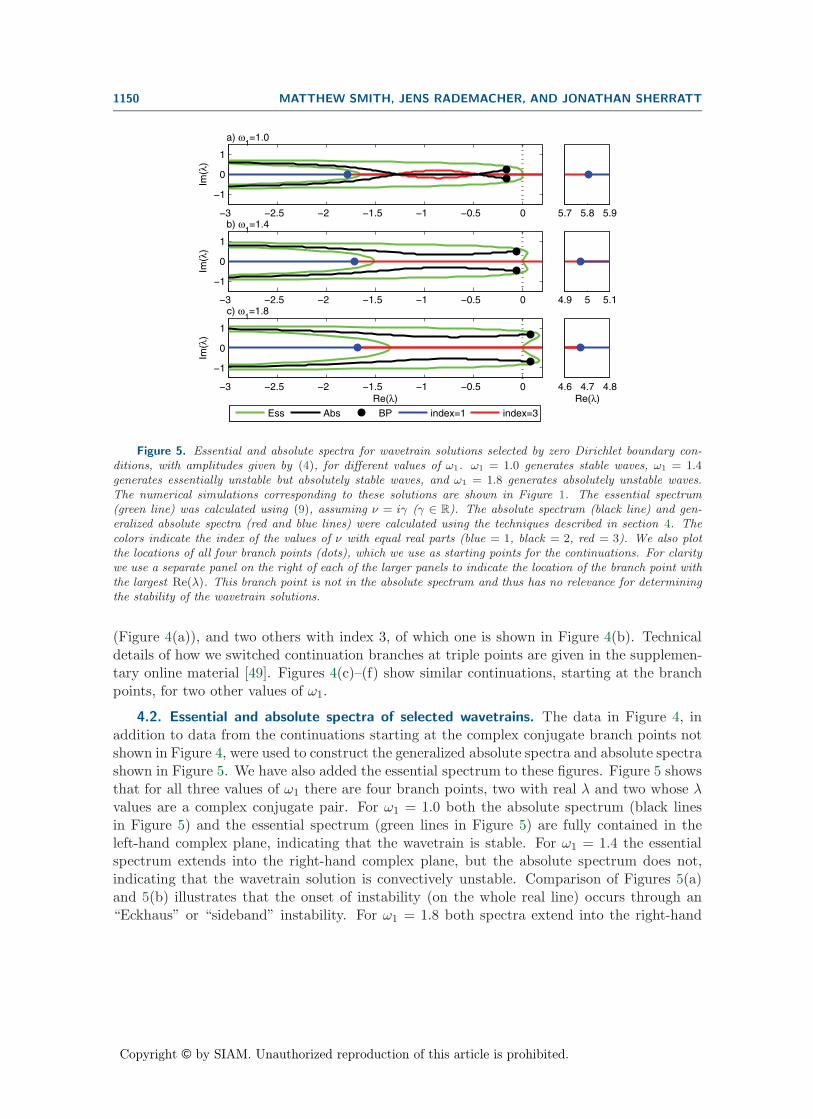
Figure 5. Essential and absolute spectra for wavetrain solutions selected by zero Dirichlet boundary con-ditions, with amplitudes given by (4), for different values of ω1. ω1 = 1.0 generates stable waves, ω1 = 1.4generates essentially unstable but absolutely stable waves, and ω1 = 1.8 generates absolutely unstable waves.The numerical simulations corresponding to these solutions are shown in Figure 1. The essential spectrum(green line) was calculated using (9), assuming ν = iγ (γ ∈ R). The absolute spectrum (black line) and gen-eralized absolute spectra (red and blue lines) were calculated using the techniques described in section 4. Thecolors indicate the index of the values of ν with equal real parts (blue = 1, black = 2, red = 3). We also plotthe locations of all four branch points (dots), which we use as starting points for the continuations. For claritywe use a separate panel on the right of each of the larger panels to indicate the location of the branch point withthe largest Re(λ). This branch point is not in the absolute spectrum and thus has no relevance for determiningthe stability of the wavetrain solutions.

(Figure 4(a)), and two others with index 3, of which one is shown in Figure 4(b). Technicaldetails of how we switched continuation branches at triple points are given in the supplemen-tary online material [49]. Figures 4(c)–(f) show similar continuations, starting at the branchpoints, for two other values of ω1.

4.2. Essential and absolute spectra of selected wavetrains. The data in Figure 4, inaddition to data from the continuations starting at the complex conjugate branch points notshown in Figure 4, were used to construct the generalized absolute spectra and absolute spectrashown in Figure 5. We have also added the essential spectrum to these figures. Figure 5 showsthat for all three values of ω1 there are four branch points, two with real λ and two whose λvalues are a complex conjugate pair. For ω1 = 1.0 both the absolute spectrum (black linesin Figure 5) and the essential spectrum (green lines in Figure 5) are fully contained in theleft-hand complex plane, indicating that the wavetrain is stable. For ω1 = 1.4 the essentialspectrum extends into the right-hand complex plane, but the absolute spectrum does not,indicating that the wavetrain solution is convectively unstable. Comparison of Figures 5(a)and 5(b) illustrates that the onset of instability (on the whole real line) occurs through an“Eckhaus” or “sideband” instability. For ω1 = 1.8 both spectra extend into the right-hand



half of the complex plane, indicating that the wavetrain is absolutely unstable and that theonset of absolute instability (again on the whole real line) occurs through a complex conjugatepair of branch points, as predicted by Corollary 3. We remark that this suggests that on largedomains with separated boundary conditions the onset of instability is of Hopf type, providedthat the boundary conditions give stable “boundary spectrum” [38].

The results shown in Figure 5 are typical for all combinations of ω1 and R that we havelooked at, except that all four λ values associated with the four different branch points arereal in some cases (see Figure 3). Trivially, the absolute spectrum has a maximum realpart for λ and extends to infinity in the left-hand half of the complex plane. Moreover,as mentioned above, in a constant coefficient case such as this, the absolute spectrum isconnected, and “isolas” cannot exist. It is possible, in general, that part of the absolutespectrum that is connected to a branch point with Re(λ) < 0 nevertheless crosses into theright-hand half of the complex plane before curving back across the imaginary axis, leadingto a “remnant” instability on large bounded domains with separated boundary conditions(see [38] for details and Figure 10 of [33] for an example). Corollary 3 shows that this cannotoccur for (1).

Crucially, the presence of the absolute spectrum in the right-hand half of the complexplane is always associated with a branch point with Re(λ) > 0. Hence as parameter values arevaried so that the selected wavetrain changes its absolute stability, this occurs via a branchpoint crossing the imaginary axis in λ. One simple consequence of this is that numericalcalculation of the full absolute spectrum is not necessary to determine whether or not a givenwavetrain is absolutely stable. Instead, one can simply calculate the positions of the fourbranch points in the complex λ plane, and the associated values of ν.

4.3. Thresholds for absolute stability. We calculated the wavetrain amplitude, R, asso-ciated with a complex conjugate pair of branch points lying on the imaginary axis, for varyingω1, using continuation in auto. This method gives the general wavetrain amplitude threshold(R) for the absolute stability of wavetrain solutions to (1) as a function of ω1. To do this weimplemented the numerical methodology described in section 4.1. We used a solution to equa-tions (13) from a known complex conjugate branch point as a starting point, and performeda continuation in R (with ω1 constant), labeling the solution at which Re(λ) = 0. We thenperformed a second continuation from this labeled solution, fixing Re(λ) = 0 and varying ω1

while tracking R. The resulting absolute stability line is plotted in Figure 6 (the thick solidline). As ω1 is increased from zero, the critical amplitude at which absolute stability changesdeclines initially before then increasing monotonically. This contrasts with the convective sta-bility threshold (derived from (3)), which increases monotonically as ω1 increases from zero(the dotted line in Figure 6).

The two general stability thresholds (“Abs” and “Ess”) in Figure 6 allow us to determinethe absolute stability and stability, respectively, for all wavetrain solutions (2) to the lambda-omega equations. In Figure 6 we overlay plots for the amplitude selected by zero Dirichletboundary conditions (“Dirichlet”) using (4) and another wave selection scenario that will bedescribed in the discussion (“Invasion”). This shows that the stability of wavetrain solutionsselected by each boundary condition changes at critical values of ω1, although the criticalvalues are different for the two different wave selection scenarios (other than when ω1 = 0).



0 1 2 3 4 5 6 7 8 9 100.4

0.5

0.6

0.7

0.8

0.9

1

ω1

wav

e am

plitu

de, r

AbsEssDirichletInvasionFig.1

Figure 6. The relationship between ω1 and the critical amplitudes of wavetrain solutions to (1), above whichwaves are essentially or absolutely unstable (dotted and thick solid lines labeled “Ess” and “Abs,” respectively).The critical amplitude for essential stability was determined using (9), and that for absolute stability was deter-mined using numerical continuation, as described in section 4. We also overlay the amplitudes of wavetrainsselected by zero Dirichlet boundary conditions (given by (4) and indicated by a thin solid line labeled “Dirichlet”)and invasion (the dashed line labeled “Invasion”); the latter is simply a different wavetrain selection scenario(with selected wavetrain amplitude given by (16)) and is discussed in section 6. The crosses indicate the valuesof ω1 used in Figure 1.

Figure 6 also shows that at ω1 = 0 wavetrains cannot be convectively unstable; rather, aninstability is always absolute (due to the additional symmetry).

We used continuation in auto to obtain an accurate estimate for the absolute stabilityparameter threshold for waves selected by zero Dirichlet boundary conditions, i.e., R = rdir,where rdir is given by (4). This is the point at which the thick solid line labeled “Abs” crossesthe thin solid line labeled “Dirichlet” in Figure 6. To obtain our estimate we performed thesame continuations as before but restricting the wavetrain amplitude, R, to be a solutionto (4). We again used one of the complex conjugate branch points as a starting point, butthis time we performed the continuation in ω1, getting auto to indicate the precise value ofω1 at which Re(λ) = 0. This gave the absolute stability threshold as ω1 < 1.576465, whichcorresponds to rdir = 0.846456.

5. Source-sink solutions. When the value of the parameter ω1 implies that zero Dirichletboundary conditions select a convectively unstable wave, the solution has the form of bandsof wavetrains with alternating directions of propagation (Figure 1(c),(d)). These bands areseparated by localized defects known as sources and sinks, with the asymptotic wavetrains



propagating away from sources and towards sinks.1 Sources and sinks have been studiedextensively in the complex Ginzburg–Landau equation; for reviews, see [56, 1, 55]. For adiscussion in the context of general oscillatory reaction-diffusion systems, see [37].

The occurrence of the alternating direction wavetrain bands for values of ω1 for which theunderlying wavetrain is convectively unstable (and thus absolutely stable) provides a clearillustration of the difference between convective and absolute stability. When the wavetrain isconvectively unstable, perturbations of an appropriate form grow with time, moving throughspace as they grow. For the lambda-omega system (1), the perturbations are moving in thesame direction as wave propagation (when ω0 > ω1 > 0). For an infinite (or sufficiently largefinite) expanse of the wavetrain, the perturbation can move and grow without constraint,destabilizing the solution. However, in the context of a source-sink pattern, the perturbationis convected as far as the nearest downstream sink, where it is completely absorbed (illustratedin Figure 7). In contrast, if the wavetrain were absolutely unstable, the perturbation wouldgrow at the site of initial application, unchecked by any surrounding sources and sinks. Thestability of solution structures composed of finite segments of convectively unstable solutionshas been established in a number of other contexts; see, for example, the work of [40, 28, 34]on pulses in reaction-diffusion systems. Very recently, Sandstede and Scheel [36] have provedthat, for the type of solution we are describing, stability depends precisely on the absolutestability of the underlying wavetrain.

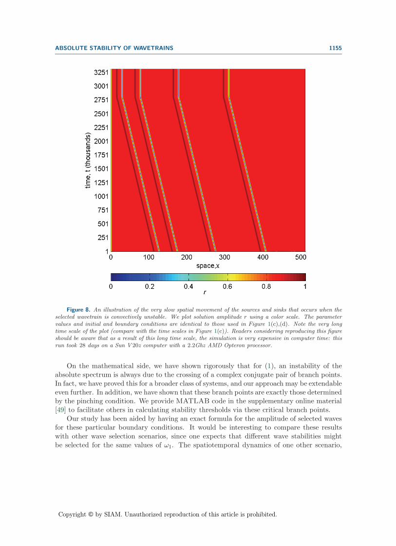
Results of Sandstede and Scheel [37, section 6.8] enable a detailed characterization ofthe repeating source-sink pattern seen in Figure 1(c),(d). Provided that the width of eachwavetrain band is large (relative to the half life of the decay of the sources and sinks to theirasymptotic wavetrains), the solution form differs only slightly from a repeating pattern ofstationary sources and sinks. Specifically, the difference is O(e−δL) for some δ > 0 as thesource-sink separation L → ∞. The exponentially small differences between the solutionsin simulations such as Figure 1(c),(d) and stationary sources/sinks have one particularlyimportant implication: the sources and sinks in our solutions move, though at an extremelyslow speed (illustrated in Figure 8).

6. Discussion. Our main focus in this study has been to derive the spectra of wavetrainsin a reaction-diffusion system of “lambda-omega” type, and to assess their utility in predictingthe dynamics emerging in partial differential equation simulations on large bounded domainswith a zero Dirichlet condition at one boundary. Our results indicate that it is possible topredict the dynamics that emerge in numerical simulations, using the wave selection formulaof [41] in combination with numerical calculation of the stability spectra of the selected wave-train. This leads us to identify three regions of parameter space with qualitatively differentdynamics: stable wave selection, which has been explained in detail elsewhere; convectively

1The distinction between sources and sinks is actually based on group velocity rather than phase velocity.These are usually defined in terms of the wavenumber k and temporal frequency Ω(k) of a wavetrain family,so that the solution is a function of kx − Ω(k)t. Then the phase velocity is Ω(k)/k, while the group velocityis dΩ(k)/dk. For the lambda-omega system (1), the wavetrain solution (u, v) = R(sin θ, cos θ) with θ ={(ω0 − ω1R

2)t ± (1 − R2)1/2x}

therefore has phase velocity ∓(ω0 − ω1R2)/(1 − R2)1/2 and group velocity

∓2ω1(1−R2)1/2. Hence our assumptions ω0 > ω1 > 0 imply that the phase and group velocities have the samesign, since R2 ≤ 1. Note, however, that if one were to take ω0 negative with −ω0 > ω1 > 0, the signs would beopposite, so that waves would propagate towards sinks and away from sources.



Figure 7. An illustration of the spatiotemporal evolution of a localized perturbation in the case of source-sink dynamics. We solved (1) on 0 < x < 512 subject to u = v = 0 at x = 0 and ux = vx = 0 at x = 512, up totime t = 3900. The parameter ω1 = 1.4, so that the resulting wavetrain is convectively unstable, and a patternof sources and sinks develops (see Figure 1(c),(d), which use the same parameter values). We then made aperturbation at one space point, increasing u and v by 0.1 at x = 194.82, and then resumed the simulation upto t = 4300. The perturbation is convected in the positive x direction as far as the nearest sink, where it iscompletely absorbed.

unstable wave selection, in which we obtain bands of wavetrains separated by localized sourcesand sinks; and absolutely unstable wave selection, in which we observe irregular spatiotem-poral dynamics.

Our subdivision of parameter space has important potential applications for predicting thespatiotemporal dynamics that will be observed in numerical simulations of other oscillatoryreaction-diffusion systems, and in nature. For instance, a topical question for oscillatoryecological systems is whether or not they exhibit periodic traveling waves [5, 47]. Our resultshere suggest that the absolute stability threshold, rather than the stability threshold, maybe more useful in predicting whether periodic traveling waves will be observed in the field.This is because the relevant ecological data is rarely, if ever, collected at sufficient spatial andtemporal resolution to identify fine details of spatiotemporal dynamics such as source/sinkdefects. Furthermore, the usual size of habitats from which data is collected is far smallerthan the domains considered here—a few spatial periods of the wavetrain would be typical.Our numerical simulations suggest that for such short domains there may be no qualitativedifference between stable and convectively unstable wavetrains.



Figure 8. An illustration of the very slow spatial movement of the sources and sinks that occurs when theselected wavetrain is convectively unstable. We plot solution amplitude r using a color scale. The parametervalues and initial and boundary conditions are identical to those used in Figure 1(c),(d). Note the very longtime scale of the plot (compare with the time scales in Figure 1(c)). Readers considering reproducing this figureshould be aware that as a result of this long time scale, the simulation is very expensive in computer time: thisrun took 28 days on a Sun V 20z computer with a 2.2Ghz AMD Opteron processor.

On the mathematical side, we have shown rigorously that for (1), an instability of theabsolute spectrum is always due to the crossing of a complex conjugate pair of branch points.In fact, we have proved this for a broader class of systems, and our approach may be extendableeven further. In addition, we have shown that these branch points are exactly those determinedby the pinching condition. We provide MATLAB code in the supplementary online material[49] to facilitate others in calculating stability thresholds via these critical branch points.

Our study has been aided by having an exact formula for the amplitude of selected wavesfor these particular boundary conditions. It would be interesting to compare these resultswith other wave selection scenarios, since one expects that different wave stabilities mightbe selected for the same values of ω1. The spatiotemporal dynamics of one other scenario,



invasion, has been studied in detail [29, 57, 42]. In this case, the boundary conditions arezero Neumann (ux = vx = 0) at both boundaries, with initial conditions consisting of a smalllocalized perturbation to the unstable steady state u = v = 0, adjacent to one boundary.Sherratt [44, 42, 43] showed that such a perturbation induces a propagating invasion front,which for (1) always has a speed of 2 [57]. A fixed invasion speed is convenient for the purposeof simulations, as it makes it straightforward to calculate the solution time and domain sizerequired to generate a given number of wavelengths.

The propagating invasion front selects the member of the periodic traveling wave family (2)with amplitude

(16) rinv ={

2ω2

1

[√1 + ω2

1 − 1]}1/2

(see [29, 57, 42]); this is slightly smaller than that selected by a zero Dirichlet boundarycondition. The properties of the spatiotemporal dynamics that emerge behind the invasionfront again depend on the stability of this wavetrain, which can be determined from Figure 6.The wave is stable for ω1 < 1.0714 and absolutely stable for ω1 < 1.5127.

In Figure 9 we show the spatiotemporal dynamics arising from invasion for three differentvalues of ω1. In all of our invasion simulations we assume that ux = vx = 0 at both boundariesof the simulated domain and make an initial perturbation of u = v = 0.1 on 0 ≤ x < 10, withu = v = 0 elsewhere.

As shown in [42], a wavetrain emerges behind the invasion front when ω1 is such that astable member of the wavetrain family is selected by invasion (Figure 9(a),(b)). In this casethe wavetrain travels in the opposite direction from the invasion front. When an unstablewavetrain is selected, we again see the wavetrain in a band behind the invasion front. However,this breaks up at a certain distance from the invasion front (Figure 9(c)–(f)). The existence of apropagating band of unstable waves behind an invasion front has been documented previouslyin numerical simulations of models for cyclic predator-prey systems [45, 46, 31, 30, 23, 19, 20,24]. The wavetrain band becomes narrower as ω1 is increased, and persists as one crosses thethreshold for absolute instability of the wavetrain; the behavior behind the band then changesfrom source-sink type (Figure 9(c),(d)) to more disordered dynamics (Figure 9(e),(f)). In arecent publication we present a method for calculating the dependence of the width of thewavetrain band on ω1 [48]. However, a more detailed investigation of the way in which theoverall solution changes with ω1 is a natural area for future work.

Acknowledgments. The work in this paper has been greatly facilitated by very helpfuldiscussions with Bjorn Sandstede (Brown University) and Leonid Brevdo (Louis Pasteur Uni-versity). We thank the Microsoft Research Cambridge Tools and Technology Group (Compu-tational Science) for technical assistance with the Lambda-Omega Equations Simulator, andtwo anonymous referees for helpful comments.



Figure 9. Example spatiotemporal dynamics for the lambda-omega equations (1) under an invasion sce-nario. Simulations started with u = v = 0 throughout the domain except u = v = 0.1 at 0 < x < 10.We fix ux = vx = 0 at both domain edges throughout the simulations. In all cases we show space-time plotsfor u and the solution amplitude r = (u2 + v2)1/2. In (a),(b) we demonstrate the selection of a stable wave(ω1 = 1.0). Parts (c)–(f) show the spatiotemporal dynamics when the selected wave is convectively unstable( (c),(d): ω1 = 1.4) and absolutely unstable ( (e),(f): ω1 = 1.8), respectively. In all cases ω0 = 3.0, and we plotu and the solution amplitude r =

√u2 + v2. For clarity, we plot the long-term solution for r as a function of

space x at one time point in (b), and show space-time plots in (a) and (c)–(f). We plot the solution across thewhole domain in (a), (b), (d), and (f), but for only part of the domain in (c),(e).

REFERENCES

[1] I. S. Aranson and L. Kramer, The world of the complex Ginzburg-Landau equation, Rev. ModernPhys., 74 (2002), pp. 99–143.

[2] I. S. Aranson, L. Aranson, L. Kramer, and A. Weber, Stability limits of spirals and traveling wavesin nonequilibrium media, Phys. Rev. A, 46 (1992), pp. R2992–R2995.

[3] J. F. G. Auchmuty and G. Nicoli, Bifurcation analysis of reaction-diffusion equations III. Chemicaloscillations, Bull. Math. Biol., 38 (1976), pp. 325–350.

[4] N. Bekki and K. Nozaki, Formations of spatial patterns and holes in the generalised Ginzburg-Landauequation, Phys. Lett., 110A (1985), pp. 133–135.

[5] O. N. Bjørnstad, R. A. Ims, and X. Lambin, Spatial population dynamics: Analyzing patterns andprocesses of population synchrony, Trends Ecol. Evol., 14 (1999), pp. 427–432.

[6] J. F. Blowey and M. R. Garvie, A reaction-diffusion system of lambda-omega type. Part I: Mathe-matical analysis, European J. Appl. Math., 16 (2005), pp. 1–19.



[7] L. Brevdo, P. Laure, F. Dias, and T. J. Bridges, Linear pulse structure and signalling in a filmflow on an inclined plane, J. Fluid Mech., 396 (1999), pp. 37–71.

[8] L. Brevdo and T. J. Bridges, Absolute and convective instabilities of temporally oscillating flows, Z.Angew. Math. Phys., 48 (1997), pp. 290–309.

[9] L. Brevdo and T. J. Bridges, Absolute and convective instabilities of spatially periodic flows, Phil.Trans. R. Soc. Lond. A, 354 (1996), pp. 1027–1064.

[10] L. Brevdo, Convectively unstable wave packets in the Blasius boundary layer, Z. Angew. Math. Mech.,75 (1995), pp. 423–436.

[11] L. Brevdo, A study of absolute and convective instabilities with an application to the Eady model, Geo-phys. Astrophys. Fluid Dynam., 40 (1988), pp. 1–92.

[12] R. J. Briggs, Electron-Stream Interaction with Plasmas, MIT Press, Cambridge, MA, 1964.[13] J. M. Chomaz, Global instabilities in spatially developing flows: Non-normality and nonlinearity, in

Annu. Rev. Fluid Mech. 37, Annual Reviews, Palo Alto, CA, 2005, pp. 357–392.[14] M. Cross and P. C. Hohenberg, Pattern formation outside of equilibrium, Rev. Modern Phys., 65

(1993), pp. 851–1112.[15] E. J. Doedel, Nonlinear numerics, J. Franklin Inst., 334 (1997), pp. 1049–1073.[16] E. J. Doedel, AUTO, A program for the automatic bifurcation analysis of autonomous systems, Congr.

Numer., 30 (1981), pp. 265–384.[17] E. J. Doedel, W. Govaerts, Y. A. Kuznetsov, and A. Dhooge, Numerical continuation of branch

points of equilibria and periodic orbits, in Modelling and Computations in Dynamical Systems, E.J. Doedel, E. J. Domokos, and I. G. Keverkidis, eds., World Scientific, River Edge, NJ, 2006, pp.145–164.

[18] G. B. Ermentrout, X. Chen, and Z. Chen, Transition fronts and localized structures in bistablereaction-diffusion equations, Phys. D, 108 (1997), pp. 147–167.

[19] M. R. Garvie, Finite-difference schemes for reaction-diffusion equations modeling predator-prey inter-actions in matlab, Bull. Math. Biol., 69 (2007), pp. 931–956.

[20] M. R. Garvie and C. Trenchea, Finite element approximation of spatially extended predator-preyinteractions with the Holling type II functional response, Numer. Math., 107 (2007), pp. 641–667.

[21] P. Huerre and P. A. Monkewitz, Local and global instabilities in spatially developing flows, in Annu.Rev. Fluid Mech. 22, Annual Reviews, Palo Alto, CA, 1990, pp. 473–537.

[22] N. Kopell and L. N. Howard, Plane wave solutions to reaction-diffusion equations, Stud. Appl. Math.,52 (1973), pp. 291–328.

[23] H. Malchow and S. V. Petrovskii, Dynamical stabilization of an unstable equilibrium in chemical andbiological systems, Math. Comput. Modelling, 36 (2002), pp. 307–319.

[24] H. Malchow, S. V. Petrovskii, and E. Venturino, Spatiotemporal Patterns in Ecology and Epidemi-ology: Theory, Models and Simulation, Chapman & Hall/CRC Press, Boca Raton, FL, 2008.

[25] The Mathworks, Version 7.6.0.324, R2008a.[26] J. D. Murray, Mathematical Biology II: Spatial Models and Biomedical Applications, Springer, New

York, 2003.[27] A. C. Newell, Envelope equations, in Nonlinear Wave Motion, Lectures in Appl. Math. 15, A. C. Newell,

ed., American Mathematical Society, Providence, RI, 1974, pp. 157–163.[28] S. Nii, The accumulation of eigenvalues in a stability problem, Phys. D, 142 (2000), pp. 70–86.[29] K. Nozaki and N. Bekki, Exact solutions of the generalised Ginzburg-Landau equation, J. Phys. Soc.

Japan, 53 (1984), pp. 1581–1582.[30] S. V. Petrovskii, K. Kawasaki, F. Takasu, and N. Shigesada, Diffusive waves, dynamical stabi-

lization and spatio-temporal chaos in a community of three competitive species, Japan J. Ind. Appl.Math., 18 (2001), pp. 459–481.

[31] S. V. Petrovskii and H. Malchow, Critical phenomena in plankton communities: kiss model revisited,Nonlinear Anal. Real World Appl., 1 (2000), pp. 37–51.

[32] J. D. M. Rademacher, Geometric relations of absolute and essential spectra of wave trains, SIAM J.Appl. Dyn. Syst., 5 (2006), pp. 634–649.

[33] J. D. M. Rademacher, B. Sandstede, and A. Scheel, Computing absolute and essential spectra usingcontinuation, Phys. D, 229 (2007), pp. 166–183.

[34] M. M. Romeo and C. K. R. T. Jones, Stability of neuronal pulses composed of concatenated unstablekinks, Phys. Rev. E, 63 (2001), paper 011904.



[35] B. Sandstede, Stability of travelling waves, in Handbook of Dynamical Systems II, B. Fielder, ed.,North-Holland, Amsterdam, 2002, pp. 983–1055.

[36] B. Sandstede and A. Scheel, Interaction of Defects, manuscript, in preparation.[37] B. Sandstede and A. Scheel, Defects in oscillatory media: Toward a classification, SIAM J. Appl.

Dyn. Syst., 3 (2004), pp. 1–68.[38] B. Sandstede and A. Scheel, Absolute and convective instabilities of waves on unbounded and large

bounded domains, Phys. D, 145 (2000), pp. 233–277.[39] B. Sandstede and A. Scheel, Absolute versus convective instability of spiral waves, Phys. Rev. E, 62

(2000), pp. 7708–7714.[40] B. Sandstede and A. Scheel, Gluing unstable fronts and backs together can produce stable pulses,

Nonlinearity, 13 (2000), pp. 1465–1482.[41] J. A. Sherratt, Periodic travelling wave selection by Dirichlet boundary conditions in oscillatory

reaction-diffusion systems, SIAM J. Appl. Math., 63 (2003), pp. 1520–1538.[42] J. A. Sherratt, On the evolution of periodic plane waves in reaction-diffusion equations of λ–ω type,

SIAM J. Appl. Math., 54 (1994), pp. 1374–1385.[43] J. A. Sherratt, On the speed of amplitude transition waves in reaction diffusion equations of λ–ω type,

IMA J. Appl. Math., 52 (1994), pp. 79–92.[44] J. A. Sherratt, The amplitude of periodic plane waves depends on initial conditions in a variety of λ–ω

systems, Nonlinearity, 6 (1993), pp. 703–716.[45] J. A. Sherratt, M. A. Lewis, and A. C. Fowler, Ecological chaos in the wake of invasion, Proc.

Natl. Acad. Sci. USA, 92 (1995), pp. 2524–2528.[46] J. A. Sherratt, B. T. Eagan, and M. A. Lewis, Oscillations and chaos behind predator-prey invasion:

Mathematical artifact or ecological reality?, Phil. Trans. R. Soc. B, 352 (1997), pp. 21–38.[47] J. A. Sherratt and M. J. Smith, Periodic travelling waves in cyclic populations: Field studies and

reaction-diffusion models, J. R. Soc. Interface, 5 (2008), pp. 483–505.[48] J. A. Sherratt, M. J. Smith, and J. D. M. Rademacher, Locating the transition from periodic

oscillations to spatiotemporal chaos in the wake of invasion, Proc. Natl. Acad. Sci. USA, 106 (2009),pp. 10890–10895.

[49] M. J. Smith, J. D. M. Rademacher, and J. A. Sherratt, Details on the computation of absolutespectra for periodic travelling waves in the Lambda-Omega equations using MATLAB and AUTO,online at http://research.microsoft.com/en-us/projects/loptw/tutorial.aspx.

[50] M. J. Smith, J. A. Sherratt, and N. J. Armstrong, The effects of obstacle size on periodic travellingwaves in oscillatory reaction-diffusion equations, Proc. R. Soc. Lond. A, 464 (2008), pp. 365–390.

[51] S. A. Suslov, Convective and absolute instabilities in non-Boussinesq mixed convection, Theoret. Comp.Fluid Dynam., 21 (2007), pp. 271–290.

[52] S. A. Suslov, Numerical aspects of searching convective/absolute instability transition, J. Comput. Phys.,212 (2006), pp. 188–217.

[53] S. A. Suslov and S. Paolucci, Stability of non-Boussinesq convection via the complex Ginzburg-Landaumodel, Fluid Dyn. Res., 35 (2004), pp. 159–203.

[54] S. A. Suslov, Searching convective/absolute instability boundary for flows with fully numerical dispersionrelation, Comput. Phys. Comm., 142 (2001), pp. 322–325.

[55] M. van Hecke, Coherent and incoherent structures in systems described by the 1D CGLE: Experimentsand identification, Phys. D, 174 (2003), pp. 134–151.

[56] W. van Saarloos, Fronts, pulses, sources and sinks in generalized complex Ginzburg-Landau equations,Phys. D, 56 (1992), pp. 303–367.

[57] W. van Saarloos, Front propagation into unstable states, Phys. Rep., 386 (2003), pp. 29–222.[58] V. K. Vanag and I. R. Epstein, Localized patterns in reaction-diffusion systems, Chaos, 17 (2007),

paper 037110.[59] P. Wheeler and D. Barkley, Computation of spiral spectra, SIAM J. Appl. Dyn. Syst., 5 (2006), pp.

157–177.

http://research.microsoft.com/en-us/projects/loptw/tutorial.aspx

absolute stability of wavetrains can explain ...jas/paperpdfs/smithrademachersherratt2009.pdf ·...

Documents