absolute stability analysis of lure’s systems and some
TRANSCRIPT
Introduction of Lure systemsStability establishment
Explore more properties using quadratic programmeConclusion
Bibliography
Absolute stability analysis of Lure’s systemsand some extensions
Guang LiSchool of Engineering, Computing and Mathematics, Exeter
6th January 2011
1 / 67

Introduction of Lure systemsStability establishment
Explore more properties using quadratic programmeConclusion
Bibliography
Outline
1 Introduction of Lure systems
2 Stability establishment
3 Explore more properties using quadratic programme
4 Conclusion
2 / 67

Introduction of Lure systemsStability establishment
Explore more properties using quadratic programmeConclusion
Bibliography
Lure’s systems
u yr = 0
+−
x = Ax + Buy = Cx
φ(·)
Figure: Lure System
Definition – Lure system
A linear time invariant (LTI) plant is connected with a nonlinearity:
The plant G(s) := (A, B, C, 0) is a minimal realization.
The nonlinearity φ(·) is memoryless, locally Lipschitz in y andsatisfies a sector (bound) condition.
3 / 67

Introduction of Lure systemsStability establishment
Explore more properties using quadratic programmeConclusion
Bibliography
Sector bound condition – SISO case
Let φ : R 7→ R with φ(0) = 0. We denote φ ∈ [k1, k2] if φ(·)satisfies
[φ(y) − k1y ][φ(y) − k2y ] ≤ 0 ∀y ∈ R (1)
-
6
y
φ(y)
φ(y) = k1y
φ(y) = k2y
Figure: Sector bound condition (SISO case)4 / 67

Introduction of Lure systemsStability establishment
Explore more properties using quadratic programmeConclusion
Bibliography
Sector bound condition – SISO case
Let φ : R 7→ R with φ(0) = 0. We denote φ ∈ [k1, k2] if φ(·)satisfies
[φ(y) − k1y ][φ(y) − k2y ] ≤ 0 ∀y ∈ R (1)
-
6
y
φ(y)
φ(y) = k1y
φ(y) = k2y
Figure: Sector bound condition (SISO case)5 / 67

Introduction of Lure systemsStability establishment
Explore more properties using quadratic programmeConclusion
Bibliography
Common nonlinearites
Saturation
-6
- -y φ(y)
Figure: Saturation
Saturation nonlinearity satisfies:
φ(y)(φ(y) − y) ≤ 0
which corresponds to the general case when k1 = 0 andk2 = 1. Denote φ ∈ [0, 1].
6 / 67

Introduction of Lure systemsStability establishment
Explore more properties using quadratic programmeConclusion
Bibliography
Common nonlinearites
Deadzone
-6
- -y φ(y)
Figure: Deadzone
Deadzone nonlinearity satisfies:
φ(y)(φ(y) − y) ≤ 0
which corresponds to the general case when k1 = 0 andk2 = 1. Denote φ ∈ [0, 1].
7 / 67

Introduction of Lure systemsStability establishment
Explore more properties using quadratic programmeConclusion
Bibliography
Sector bound condition – Multivariable Case
Diagonal case:
[φ(y) − K1y ]T [φ(y) − K2y ] ≤ 0
where K1 and K2 are diagonal matrices with K1 − K2 < 0and
y =
y1
y2...
ym
φ(y) =
φ1(y1)φ2(y2)
...φm(ym)
Coupled case:
[φ(y) − K1y ]T [φ(y) − K2y ] ≤ 0
where K1 and K2 are positive definite matrices withK1 − K2 < 0, and φi(y) can depend on yj .
8 / 67

Introduction of Lure systemsStability establishment
Explore more properties using quadratic programmeConclusion
Bibliography
A Lure’s system
u yr = 0
+−
x = Ax + Buy = Cx
φ(·)
Figure: A Lure System
Definition – Absolute stability [Khalil(2000)]
Suppose φ satisfies a sector condition. The system isabsolutely stable if the equilibrium point at the origin is globallyuniformly asymptotically stable for any nonlinearity in the givensector.
9 / 67

Introduction of Lure systemsStability establishment
Explore more properties using quadratic programmeConclusion
Bibliography
Outline
1 Introduction of Lure systems
2 Stability establishment
3 Explore more properties using quadratic programme
4 Conclusion
10 / 67

Introduction of Lure systemsStability establishment
Explore more properties using quadratic programmeConclusion
Bibliography
Some Classical Stability Criteria
There are a number of classical criteria for the absolute stabilityanalysis of the Lure system:
Circle criterion;
Popov criterion;
Zames-Falb multiplier theory [Zames and Falb(1968)];
Small gain;
Passivity theory;
· · ·
These criteria are related to each other.Two key problems to investigate:
Less conservative?
Easier to use?11 / 67

Introduction of Lure systemsStability establishment
Explore more properties using quadratic programmeConclusion
Bibliography
the S-procedure
the S-procedure [Yakubovich(1971)]
Suppose there are two statements as:
S1: σ1 ≥ 0, σ2 ≥ 0, . . . , σn ≥ 0 ⇒ σ0 ≤ 0
S2: σ0 +
N∑
i=1
τiσi ≤ 0
with τi ≥ 0, i = 1, . . . , N. It is obvious that S2 ⇒ S1. But it isnot always true that S1 ⇒ S2. It is called lossless if S1 ⇔ S2.
We are concerned about the case when σk take the quadraticforms as
σk (f ) = 〈Φk f , f 〉, k = 0, 1, . . . , N. (2)
with Φ∗k = Φk . 12 / 67

Introduction of Lure systemsStability establishment
Explore more properties using quadratic programmeConclusion
Bibliography
Using the S-procedure to establish stability
Suppose we have chosen a Lyapunov function candidateV > 0.If we denote σ0 := V (x) < 0 and use σi ≥ 0 with i = 1, . . . , N todescribe the N quadratic constraints derived from thenonlinearity in the Lure system. Then a sufficient condition forthe system to be stable is the satisfaction of the inequality:
σ0 +N∑
i=1
τiσi < 0 (3)
with τi ≥ 0 and i = 1, . . . , N.
13 / 67

Introduction of Lure systemsStability establishment
Explore more properties using quadratic programmeConclusion
Bibliography
Using the S-procedure to establish stability
We are interested in the question: how to reduce theconservatism of the stability criterion.
We have two options in this direction:
Choose different Lyapunov function candidates;
Use more constraints describing the nonlinearity.
14 / 67

Introduction of Lure systemsStability establishment
Explore more properties using quadratic programmeConclusion
Bibliography
Circle Criterion
Suppose φ ∈ [0, K ]. Then the sector condition is[xu
]T
Πc
[xu
]
≥ 0
with
Πc =
[0 −CT K T
−KC −2I
]
Choose a Lyapunov function V (x) = xT Px , with P > 0. Thesystem is g.a.s., if under the sector condition, we have
V (x) =
[xu
]T
Πv
[xu
]
< 0
with
Πv =
[AT P + PA PB
BT P 0
]
15 / 67

Introduction of Lure systemsStability establishment
Explore more properties using quadratic programmeConclusion
Bibliography
Circle Criterion
Then the Circle criterion can be derived by the S-procedure:
Πv + Πc =
[AT P + PA PB − CT K T
BT P − KC −2I
]
< 0 (4)
This is a linear matrix inequality (LMI).The feasibility of an LMI can be tested easily using some exiting LMIsolvers, such as LMILAB (a toolbox of MATLAB), SEDUMI, etc.
16 / 67

Introduction of Lure systemsStability establishment
Explore more properties using quadratic programmeConclusion
Bibliography
Popov Criterion – with positive multiplier
Choose the candidate Lyapunov function (Lure and Postnikovtype) as
V (x) = xT Px + 2r∫ y
0φ(τ)dτ (5)
with r > 0 and P > 0. The derivative of V (x) is
V (x) =
[xu
]T
(Πv + rΠp)
[xu
]
< 0 (6)
with
Πp = −
[0 AT CT
CA CB + BT CT
]
(7)
17 / 67

Introduction of Lure systemsStability establishment
Explore more properties using quadratic programmeConclusion
Bibliography
Popov Criterion – with positive multiplier
Then the Popov criterion can be derived by the S-procedure:
Πv +Πc+rΠp =
[AT P + PA PB − CT K T − rAT CT
BT P − KC − rCA −2I − r(CB + BT CT )
]
< 0
(8)
18 / 67

Introduction of Lure systemsStability establishment
Explore more properties using quadratic programmeConclusion
Bibliography
Popov Criterion – with indefinite multiplier (SISO)
Choose the candidate Lyapunov function as
V (x) = xT Px + 2r+
∫ y
0φ(τ)dτ + 2r−
∫ y
0[K τ − φ(τ)]dτ (9)
with r+ > 0, r− > 0 and P > 0. The derivative of V (x) is
V (x) =
[xu
]T
(Πv + r+Πp+ + r−Πp−)
[xu
]
< 0 (10)
with
Πp+ = −
[0 AT CT
CA CB + BT CT
]
(11)
Πp− = −
[(KC)T CA + (CA)T KC (KC)T CB
(CB)T KC 0
]
(12)
19 / 67

Introduction of Lure systemsStability establishment
Explore more properties using quadratic programmeConclusion
Bibliography
Popov Criterion – with indefinite multiplier (SISO)
Then the Popov criterion can be derived by the S-procedure:
Πv + Πc + r+Πp+ + r−Πp− < 0 with r+, r− ≥ 0 (13)
which can be (in some cases) shown equivalent to
Πv + Πc + rΠp+ < 0 (14)
with r ∈ R.
For SISO case, the equivalence can be shown by looptransformation [Yakubovich(1967)];
Diagonal MIMO case is shown in[Yakubovich(1967), Park(1997)];
Coupled MIMO case is shown in [Heath and Li(2009)].
20 / 67

Introduction of Lure systemsStability establishment
Explore more properties using quadratic programmeConclusion
Bibliography
Choice of Lyapunov Function candidates
To summarize, we have used the same sector bound conditionand chosen three different Lyapunov functions for three cases:
CircleV (x) = xT Px
Popov (positive multiplier)
V (x) = xT Px + 2r∫ y
0φ(τ)dτ
Popov (indefinite multiplier)
V (x) = xT Px + 2r+
∫ y
0φ(τ)dτ + 2r−
∫ y
0[K τ − φ(τ)]T dτ
21 / 67

Introduction of Lure systemsStability establishment
Explore more properties using quadratic programmeConclusion
Bibliography
The Criteria in Frequency Domain
Using the Kalman- Yakubovich-Popov (KYP) Lemma, thesecriteria in the LMI forms can be transformed into frequencydomain:
CircleRe{KG(jω) + I} ≥ 0 ∀ω ∈ R
Popov (positive multiplier)
Re{(K + rjωI)G(jω) + I} ≥ 0 ∀ω ∈ R
with r ≥ 0.Popov (indefinite multiplier)
Re{(K + rjωI)G(jω) + I} ≥ 0 ∀ω ∈ R
with r ∈ R.22 / 67

Introduction of Lure systemsStability establishment
Explore more properties using quadratic programmeConclusion
Bibliography
Example 1
x = Ax + Buy = Cx
r = 0+−
u y
k
Figure: Absolute stability example
A =
−2 −2 −11 0 00 1 0
B =
100
C =[1 0 0
]
23 / 67

Introduction of Lure systemsStability establishment
Explore more properties using quadratic programmeConclusion
Bibliography
Example 1
x = Ax + Buy = Cx
r = 0+−
u y
k
Figure: Absolute stability example
The rang of k > 0 that guarantees the stability of the system:
Circle: k ≤ 8.12;
Popov – positive multiplier: k ≤ 8.12;
Popov – indefinite multiplier: k ≤ 8.9.24 / 67

Introduction of Lure systemsStability establishment
Explore more properties using quadratic programmeConclusion
Bibliography
Using the S-procedure to establish stability
We are interested in the question: how to reduce theconservatism of the stability criterion.
We have two options in this direction:
Choose different Lyapunov function candidates;
Use more constraints describing the nonlinearity.
25 / 67

Introduction of Lure systemsStability establishment
Explore more properties using quadratic programmeConclusion
Bibliography
The constraints of the nonlinearity
D – The nonlinearity.
D
26 / 67

Introduction of Lure systemsStability establishment
Explore more properties using quadratic programmeConclusion
Bibliography
The constraints of the nonlinearity
D – The nonlinearity.C1 – The constraint σ1 ≥ 0.
D
27 / 67

Introduction of Lure systemsStability establishment
Explore more properties using quadratic programmeConclusion
Bibliography
The constraints of the nonlinearity
D – The nonlinearity.C1, C2 – The constraints σi ≥ 0 with i = 1, 2 respectively.
C2 D
28 / 67

Introduction of Lure systemsStability establishment
Explore more properties using quadratic programmeConclusion
Bibliography
The constraints of the nonlinearity
D – The nonlinearity.C1, C2, C3 – The constraints σi ≥ 0 with i = 1, 2, 3respectively.
C2
C3
D
29 / 67

Introduction of Lure systemsStability establishment
Explore more properties using quadratic programmeConclusion
Bibliography
The constraints of the nonlinearity
D – The nonlinearity.C1, C2, C3, C4 – The constraints σi ≥ 0 with i = 1, 2, 3, 4respectively.
C2
C3
C4
D
30 / 67

Introduction of Lure systemsStability establishment
Explore more properties using quadratic programmeConclusion
Bibliography
The constraints of the nonlinearity
D – The nonlinearity.C1, C2, C3, C4, C5 – The constraints σi ≥ 0 withi = 1, 2, 3, 4, 5 respectively.
C2
C3
C4C5
D
31 / 67

Introduction of Lure systemsStability establishment
Explore more properties using quadratic programmeConclusion
Bibliography
Outline
1 Introduction of Lure systems
2 Stability establishment
3 Explore more properties using quadratic programme
4 Conclusion
32 / 67

Introduction of Lure systemsStability establishment
Explore more properties using quadratic programmeConclusion
Bibliography
Using quadratic programme to express nonlinearities
x = Ax + Buy = Cx
r = 0++
u y
QuadraticProgram
The nonlinearity φ(·) can be expressed by a quadratic program(QP) [Primbs(2001)]:
u(t) = φ(y(t)) = arg minu
12
uT Hu + uT y(t)
subject to Lu + My � b(15)
33 / 67

Introduction of Lure systemsStability establishment
Explore more properties using quadratic programmeConclusion
Bibliography
Common nonlinearities
Saturation
-6
- -y φ(y)
Figure: Saturation
Saturation nonlinearity can be described by
u = arg minu
12
(u − y)2
s.t.|u| ≤ 1(16)
which corresponds to the QP with H = 1, F = −1, L = 1, N = 0and b = 1.
34 / 67

Introduction of Lure systemsStability establishment
Explore more properties using quadratic programmeConclusion
Bibliography
Common nonlinearities
Deadzone
-6
- -y φ(y)
Figure: Saturation
Saturation nonlinearity can be described by
u = arg minu
12
u2
s.t.|u − y | ≤ 1(17)
which corresponds to the QP with H = 1, F = 0, L = 1, N = −1and b = 1.
35 / 67

Introduction of Lure systemsStability establishment
Explore more properties using quadratic programmeConclusion
Bibliography
Using quadratic programme to express nonlinearities
x = Ax + Buy = Cx
r = 0++
u y
QuadraticProgram
The nonlinearity φ(·) can be expressed by a quadratic program(QP) [Primbs(2001)]:
u(t) = φ(y(t)) = arg minu
12
uT Hu + uT y(t)
subject to Lu + My � b(18)
36 / 67

Introduction of Lure systemsStability establishment
Explore more properties using quadratic programmeConclusion
Bibliography
Using quadratic programme to express nonlinearities
We can derive its KKT (Karush-Kuhn-Tucker) conditions:
Hu + Fy + LT λ = 0 (19a)
Lu + My + s = b (19b)
λT s = 0 (19c)
λ � 0 (19d)
s � 0 (19e)
where λ is the Lagrangian multiplier and s is the slack variable.The KKT conditions are the necessary and sufficient conditionsfor the solution of the QP to be optimal.
37 / 67

Introduction of Lure systemsStability establishment
Explore more properties using quadratic programmeConclusion
Bibliography
Using quadratic programme to express nonlinearities
From these KKT conditions and there first derivatives, we canderive three quadratic conditions[Li et al.(2007)Li, Heath, and Lennox][Li et al.(2008)Li, Heath, and Lennox]:
(u + L†My)T (Hu + Fy) − ((I − LL†)My)T λ ≤ 0 (20a)
(u + L†My)T (Hu + Fy) − ((I − LL†)My)T λ = 0 (20b)
(u + L†My)T (Hu + Fy) − ((I − LL†)My)T λ = 0 (20c)
where L† := (LT L)−1LT . The columns of L are linearlyindependent.
38 / 67

Introduction of Lure systemsStability establishment
Explore more properties using quadratic programmeConclusion
Bibliography
Using quadratic programme to express nonlinearities
From these KKT conditions and there first derivatives, we canderive three quadratic conditions[Li et al.(2007)Li, Heath, and Lennox][Li et al.(2008)Li, Heath, and Lennox]:
(u + L†My)T (Hu + Fy)−((I − LL†)My)T λ ≤ 0 (20a)
(u + L†My)T (Hu + Fy)−((I − LL†)My)T λ = 0 (20b)
(u + L†My)T (Hu + Fy)−((I − LL†)My)T λ = 0 (20c)
where L† := (LT L)−1LT . The columns of L are linearlyindependent.
39 / 67

Introduction of Lure systemsStability establishment
Explore more properties using quadratic programmeConclusion
Bibliography
Using quadratic programme to express nonlinearities
Assuming M = LN, three quadratic conditions can be furthersimplified:
(u + Ny)T (Hu + Fy) ≤ 0 (21a)
(u + Ny)T (Hu + Fy) = 0 (21b)
(u + Ny)T (Hu + Fy) = 0 (21c)
where y = Cx and y = Cx = CAx + CBu.
40 / 67

Introduction of Lure systemsStability establishment
Explore more properties using quadratic programmeConclusion
Bibliography
Common nonlinearities
Saturation
-6
- -y φ(y)
Figure: Saturation
Its quadratic constraints are:
u(u − y) ≤ 0 (22)
u(u − y) = 0 (23)
u(u − y) = 0 (24)
41 / 67

Introduction of Lure systemsStability establishment
Explore more properties using quadratic programmeConclusion
Bibliography
Common nonlinearities
Deadzone
-6
- -y φ(y)
Figure: Saturation
Its quadratic constraints are:
u(u − y) ≤ 0 (25)
u(u − y) = 0 (26)
u(u − y) = 0 (27)
42 / 67

Introduction of Lure systemsStability establishment
Explore more properties using quadratic programmeConclusion
Bibliography
Using quadratic programme to express nonlinearities
Assuming M = LN, three quadratic conditions can be furthersimplified:
(u + Ny)T (Hu + Fy) ≤ 0 (28a)
(u + Ny)T (Hu + Fy) = 0 (28b)
(u + Ny)T (Hu + Fy) = 0 (28c)
where y = Cx and y = Cx = CAx + CBu.
43 / 67

Introduction of Lure systemsStability establishment
Explore more properties using quadratic programmeConclusion
Bibliography
Using quadratic programme to express nonlinearities
Denote v := [xT , uT , uT ]T , then the three quadratic conditionscan be expressed as
vT Π1v ≥ 0 (29a)
vT Π2v = 0 (29b)
vT Π3v = 0 (29c)
with
Π1 = −He([
NC I 0] [
FC H 0])
(30a)
Π2 = He([
NCA NCB I] [
FC H 0])
(30b)
Π3 = He([
NCA NCB I] [
FCA FCB H])
(30c)
Here He(M) = M∗ + M.44 / 67

Introduction of Lure systemsStability establishment
Explore more properties using quadratic programmeConclusion
Bibliography
Using quadratic programme to express nonlinearities
Choose a candidate Lyapunov function
V (x , u) = [xT , uT ]P[xT , uT ]T (31)
with P > 0. The first derivative of V is
V (x , u) =
xuu
T
AT P11 + P11A AT P12 + P11B P12
PT12A + BT P11 PT
12B + BT P12 P22
PT12 P22 0
︸ ︷︷ ︸
Πv
xuu
(32)that is
V (x , u) = vT Πv v (33)
45 / 67
Introduction of Lure systemsStability establishment
Explore more properties using quadratic programmeConclusion
Bibliography
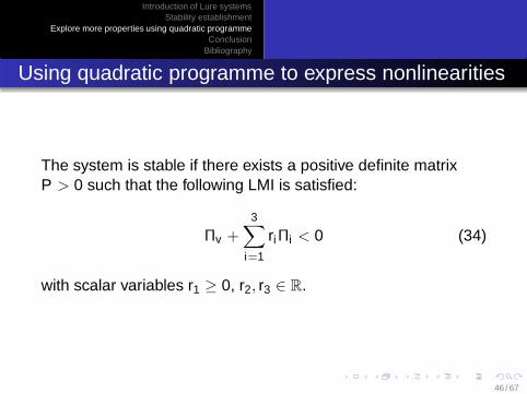
Using quadratic programme to express nonlinearities
The system is stable if there exists a positive definite matrixP > 0 such that the following LMI is satisfied:
Πv +3∑
i=1
riΠi < 0 (34)
with scalar variables r1 ≥ 0, r2, r3 ∈ R.
46 / 67

Introduction of Lure systemsStability establishment
Explore more properties using quadratic programmeConclusion
Bibliography
Example 1 – continued
x = Ax + Buy = Cx
r = 0+−
u y
k
Figure: Absolute stability example
A =
−2 −2 −11 0 00 1 0
B =
100
C =[1 0 0
]
47 / 67

Introduction of Lure systemsStability establishment
Explore more properties using quadratic programmeConclusion
Bibliography
Example 1 – continued
x = Ax + Buy = Cx
r = 0+−
u y
k
Figure: Absolute stability example
The rang of k > 0 that guarantees the stability of the system:Circle: k ≤ 8.12;Popov (indefinite multiplier): k ≤ 8.9;QP method: k < +∞.Zames-Falb multiplier: k < +∞;
48 / 67

Introduction of Lure systemsStability establishment
Explore more properties using quadratic programmeConclusion
Bibliography
Example 2
Two cases for the nonlinearity φ: saturation or deadzone;Two cases for the plant
G1(s) =1
s4 + s3 + 8s2 + 2s + 1
G2(s) =1
s4 + s3 + 8s2 + 3s + 1
Two Lyapunov function candidates:
V1(x , u) = [xT , uT ]P[xT , uT ]
V2(x , u) = [xT , uT ]P[xT , uT ] + r∫ y
0φ(τ)dτ with r ≥ 0
Note: V2 is inspired by the Lyapunov function corresponding to the Popov
criterion.
49 / 67

Introduction of Lure systemsStability establishment
Explore more properties using quadratic programmeConclusion
Bibliography
Example 2
Table: A comparison of the existing approaches and the newapproach: continuous case. In each case the maximum value of K forwhich the system is guaranteed stable is shown.
φ Plant Circle Popov QP (V1) QP (V2)sat G1 1.69 4.03 3.98 9.63dz G2 2.94 5.41 6.93 11.56dz G1 1.69 1.69 10.16 10.16
50 / 67

Introduction of Lure systemsStability establishment
Explore more properties using quadratic programmeConclusion
Bibliography
Extension to stability analysis of model predictivecontrol (MPC)
Discrete version
The stability analysis based on quadratic programme has adiscrete time version.
Extension to MPC analysis
MPC resolves a constrained optimization problem at eachsampling instant. The optimization can be expressed as a QP.Hence we can extend this method to MPC analysis.
51 / 67

Introduction of Lure systemsStability establishment
Explore more properties using quadratic programmeConclusion
Bibliography
Extension to stability analysis of model predictivecontrol (MPC)
MPC controller – minimization of cost function
An optimization problem is resolved at each sampling instant k
U∗k = arg min
Uk
xk+NpSxk+Np +
Np−1∑
i=0
[
xTk+iQxk+i + uT
k+iRuk+i
]
s.t.Lkuk � bk with bk � 0(35)
where Uk = [uTk , uT
k+1, . . . , uTk+Np−1] is the optimizer. Only the
first element of U∗k , i.e. u∗
k , is used as the control input.
52 / 67

Introduction of Lure systemsStability establishment
Explore more properties using quadratic programmeConclusion
Bibliography
Extension to robustness analysis of model predictivecontrol (MPC)
MPC controller – quadratic programme
If only input constraints are considered, the MPC optimizationproblem can be written as a quadratic programme
U∗k = arg min
Uk
UTk HUk + F T
k Uk
s.t.LUk � b with b � 0(36)
where H is a positive definite Hessian matrix, and Fk containsthe estimated or measured state xk .
53 / 67
Introduction of Lure systemsStability establishment
Explore more properties using quadratic programmeConclusion
Bibliography
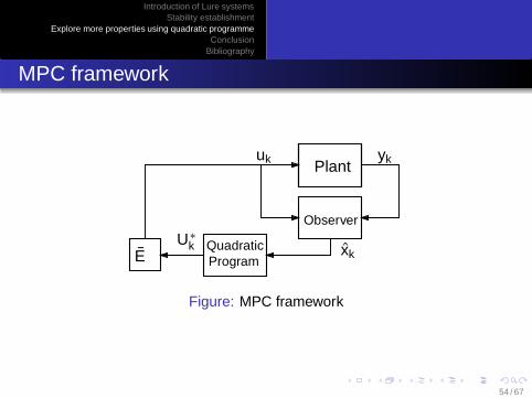
MPC framework
Plant
Observer
EQuadraticProgram
uk yk
U∗k xk
Figure: MPC framework
54 / 67

Introduction of Lure systemsStability establishment
Explore more properties using quadratic programmeConclusion
Bibliography
Example 3 – Robustness analysis of MPC
Plant
EQuadraticProgram
uk xk
U∗k
∆k
qk pk
Figure: MPC framework
55 / 67

Introduction of Lure systemsStability establishment
Explore more properties using quadratic programmeConclusion
Bibliography
Example 3 – Robustness analysis of MPC
An MPC example with uncertainties
Suppose a plant with unstructured uncertainties is
xk+1 = Axk + Buuk + Bwwk
pk = Cxk + Duuk + Dwwk
wk = ∆kpk
where ∆k satisfies‖∆k‖2 ≤ 1
with
A =
[4/3 −2/31 0
]
Bu =[1 0
]Bw =
[θ 0
]
C =[1 0
]Du = 0 Dw = 0
56 / 67

Introduction of Lure systemsStability establishment
Explore more properties using quadratic programmeConclusion
Bibliography
Example 3 – Robustness analysis of MPC
The plant is subject to input constraints |u| ≤ 1.The cost function is chosen as
U∗k = arg min
Uk
xk+NpSxk+Np +
Np−1∑
i=0
[
xTk+iQxk+i + uT
k+iRuk+i
]
s.t.Lkuk � bk with bk � 0(37)
with
Q =
[1 −2/3
−2/3 3/2
]
R = 1 S = Q Np = 3
57 / 67

Introduction of Lure systemsStability establishment
Explore more properties using quadratic programmeConclusion
Bibliography
Example 3 – Robustness analysis of MPC
The Lyapunov function is chosen to be
V = [xTk , UT
k ]T P[xTk , UT
k ]
We use the three constraints derived from the QP and thequadratic constraints from the uncertainty ‖∆k‖ ≤ 1 toestablish stability by the S-procedure.The range of θ for the system to be stable is 0 ≤ θ ≤ 0.19.
58 / 67

Introduction of Lure systemsStability establishment
Explore more properties using quadratic programmeConclusion
Bibliography
Outline
1 Introduction of Lure systems
2 Stability establishment
3 Explore more properties using quadratic programme
4 Conclusion
59 / 67
Introduction of Lure systemsStability establishment
Explore more properties using quadratic programmeConclusion
Bibliography
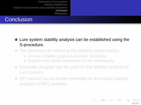
Conclusion
Lure system stability analysis can be established using theS-procedure.Two directions for reducing the stability conservatism:
Choose suitable Lyapunov function candidate;Exploit more useful constraints for the nonlinearity.
Quadratic program can be used for the stability analysis ofLure system.
QP method can be further extended for the robust stabilityanalysis of MPC systems.
60 / 67

Introduction of Lure systemsStability establishment
Explore more properties using quadratic programmeConclusion
Bibliography
Conclusion
Lure system stability analysis can be established using theS-procedure.Two directions for reducing the stability conservatism:
Choose suitable Lyapunov function candidate;Exploit more useful constraints for the nonlinearity.
Quadratic program can be used for the stability analysis ofLure system.
QP method can be further extended for the robust stabilityanalysis of MPC systems.
61 / 67

Introduction of Lure systemsStability establishment
Explore more properties using quadratic programmeConclusion
Bibliography
Conclusion
Lure system stability analysis can be established using theS-procedure.Two directions for reducing the stability conservatism:
Choose suitable Lyapunov function candidate;Exploit more useful constraints for the nonlinearity.
Quadratic program can be used for the stability analysis ofLure system.
QP method can be further extended for the robust stabilityanalysis of MPC systems.
62 / 67

Introduction of Lure systemsStability establishment
Explore more properties using quadratic programmeConclusion
Bibliography
Conclusion
Lure system stability analysis can be established using theS-procedure.Two directions for reducing the stability conservatism:
Choose suitable Lyapunov function candidate;Exploit more useful constraints for the nonlinearity.
Quadratic program can be used for the stability analysis ofLure system.
QP method can be further extended for the robust stabilityanalysis of MPC systems.
63 / 67

Introduction of Lure systemsStability establishment
Explore more properties using quadratic programmeConclusion
Bibliography
Conclusion
Lure system stability analysis can be established using theS-procedure.Two directions for reducing the stability conservatism:
Choose suitable Lyapunov function candidate;Exploit more useful constraints for the nonlinearity.
Quadratic program can be used for the stability analysis ofLure system.
QP method can be further extended for the robust stabilityanalysis of MPC systems.
64 / 67

Introduction of Lure systemsStability establishment
Explore more properties using quadratic programmeConclusion
Bibliography
Conclusion
Lure system stability analysis can be established using theS-procedure.Two directions for reducing the stability conservatism:
Choose suitable Lyapunov function candidate;Exploit more useful constraints for the nonlinearity.
Quadratic program can be used for the stability analysis ofLure system.
QP method can be further extended for the robust stabilityanalysis of MPC systems.
65 / 67

Introduction of Lure systemsStability establishment
Explore more properties using quadratic programmeConclusion
Bibliography
W.P. Heath and Guang Li.Lyapunov functions for the multivariable popov criterionwith indefinite multipliers.Automatica, 45(12):2977 – 2981, 2009.
H. K. Khalil.Nonlinear systems (3rd ed).Pearson Prentice-Hall, Upper Saddle River, 2000.
G. Li, W. P. Heath, and B. Lennox.Concise stability conditions for systems with staticnonlinear feedback expressed by a quadratic program.IET Control Theory Appl., 2(7):554–563, 2008.
Guang Li, W.P. Heath, and B. Lennox.An improved stability criterion for a class of lure systems.
66 / 67

Introduction of Lure systemsStability establishment
Explore more properties using quadratic programmeConclusion
Bibliography
In Decision and Control, 46th IEEE Conference on, pages4483 –4488, 2007.
Poogyeon Park.A revisited popov criterion for nonlinear lur’e systems withsector-restrictions.International Journal of Control, 68(3):461–470, 1997.
J. A. Primbs.The analysis of optimization based controllers.Automatica, 37:933–938, 2001.
V. A. Yakubovich.Frequency conditions for the absolute stability of controlsystems with several nonlinear or lienar nonstationaryblocks.Automation and Remote Control, 28:857–880, 1967.
67 / 67

Introduction of Lure systemsStability establishment
Explore more properties using quadratic programmeConclusion
Bibliography
V. A. Yakubovich.S-procedure in nonlinear control theory.Vestnik Leningrad University, 28:62–77, 1971.English translation in Vestnik Lenintrad University vol. 4, pp73-93.
G. Zames and P. L. Falb.Stability conditions for systems with monotone andslope-restricted nonlinearities.SIAM J. Control, 6:89–108, 1968.
68 / 67