abdul-hamid ai-ta}'>'ib may
TRANSCRIPT

NSF/RA-800219
Geometrically Nonlinear Analysis of RectangularGlass Plates by the Finite Element Method
Abdul-Hamid J. AI-Ta}'>'ib
May.1980
Institute for Disaster Research
TEXAS TECH UNIVERSITYLubbocl~, Texas 79409
REPRODUCED BYNATIONAL TECHNiCALINfORMATION SERVICE
U S DEPARTMENT OF COMMERCE•• SPIUNGF.\ElD, VA. 22151
EAS INFORMATION RESOURCESNATIONAL SCIENCE FoUNDATION


GEOMETRICALLY NONLINEAR ANALYSIS OFRECTANGULAR GLASS PLATES BY THE
FINITE ELEMENT METHOD
by
Abdul-Hamid J. Al-Tayyib
Institute for Disaster ResearchTexas Tech UniversityLubbock, Texas 79409
May, 1980
Any opinions, findings, conclusionsor recommendations expressed in thispublication are those of the author(s)and do not necessarily reflect the viewsof the National Science Foundation.


FOREWORD
The work reported herein was conducted as a part of a continuing
program of research involving engineered window glass at Texas Tech
University. The program is administered/through the Institute for Disaster
Research in the College of Engineering.
The specific project on the analysis of rectangular glass plates was
directed by Or. C. V. G. Vallabhan. The principal investigator was
Or. Abdul-Hamid J. Al-Tayyib. The project was supported by the National
Science Foundation under Award No. PFR 77-24063, the Institute for Disaster
Research, and the Department of Civil Engineering at Texas Tech University.
This report was adapted for publication by Or. J. E. Minor and W. L. Beason
from Or. Al-Tayyib's dissertation entitled, "Geometrically Nonlinear Analysis
of Rectangular Glass Panels by the Finite Element Method. II This editing was
performed so that terminology used in this publication will be consistent
with other lOR publications in the glass area. Any opinions, findings, and
conclusions or recommendations expressed in this pUblication are those of
the author and editors, and do not necessarily reflect the views of the
National Science Foundation.
i i

ACKNOWLEDGMENTS
The author is deeply indebted to Dr. C. ~. Girija Vallabhan for
his valuable assistance, guidance, and constructive criticism given
during the course of this investigation. Appreciation is also
expressed to Drs. M. M. Ayoub, K. C. Mehta, J. H. Smith, J. E. Minor,
and W. P. Vann for their helpful suggestions.
In addition, deep gratitude is expressed by the author to the
Saudi Arabian government for supporting his wish to broaden his know
ledge in the field of Civil Engineering. Finally, the author wishes
to make special mention of the generous amount of computer time pro
vided by the Department of Civil Engineering at Texas Tech University
during the development of the computer program which is a part of
this work.
iii

ABSTRACT
The primary objective of this study is to develop a finite element
model for the stress analysis of geometrically nonlinear, simply supported,
uniformly loaded, rectangular plates. Actual framing configurations for
glass plates a110wthec boundary edges to move in the plane of the plate with
little restrain. In such a situation, when the loads become large, membrane
behavior plays a significant role in changing the overall behavior of the
glass plate. In this investigation, the geometric nonlinearity treated is
that associated with large lateral elastic displacements which induce
stretching of the middle surface of the plate. The formulation is not
restricted by the magnitude of the displacements, as is linear plate theory,
provided that engineering strains do not exceed the proportional limit and
structural instability does not occur.
A finite element program which includes a nonlinear thin plate formu
lation is developed. The formulation uses a rectangular finite element with
displacement fields depicted by shape functions which are products of one
dimensional Hermitian polynomials of order one. These functions are used to
represent both membrane and bending behaviors. A 48 degree of freedom
element results, with linear and nonlinear stiffness matrices which are
derived from a purely geometric standpoint. Thirty-two of the 48 degrees
of freedom are allowed to represent the membrane behavior of the plate. This
representation of membrane behavior is important in studying stress distri
butions in glass plates, particularly at the glass plate perimeter. The
system equilibrium equations are then formulated and solved using a
Langrangian type linear incremental approach.
iv
Example problems, for which pUblished experimental and theoretical
results are available in the literature, are solved to demonstrate the
validity and versatility of the finite element formulation. In these
example problems, theoretical bending and membrane stresses are compared
separately to better assess membrane behavior in plates with large displace
ments. The glass plate problem with boundary edges that are simply supported
and free to move in the plane of the plate are analyzed and force-displacement
results are compared with independent experimental data. Computer displace
ments agree well with the experimental data.
Numerical studies conducted on the glass plate problem reveal that con
vergence differs between bending and membrane stresses, and depends upon the
fineness of the finite element discretization, the location within the plate,
and the relative magnitude of the loading increment.. This observation, in
the author1s opinion, is valuable for anyone involved in analyzing geometri
cally nonlinear thin plate problems.
v

TABLE OF CONTENTS
Page
LIST OF ILLUSTRATIONS...................................... ix
LIST OF TABLES............................................. xi
LIST OF SyMBOLS •..•••.•..•••..••.••..••.....••..••• e........ xii
1. INTRO-DUCTION. . . . . . • . . • • . . • . • . • . . • . • . . . . . . . . . . . .. • .. .. • .. .. .. .. 1
1.1 Initiation of the Problem......................... 1
1.2 Definition of the Problem •.••••.•••••.••.•.•.••••• 1
1. 3 Previous and Current Work......................... 3
1.4 Approach . . .. .. . . . .. . . . .. .. . .. .. .. . . .. . . .. .. .. . . 5
1.5 Objective and Scope of Research ..•••...••.•••••••• 5
2. lARGE DEFLECTION THEORY OF THIN PLATES .•....•.•........ 8
2.1 Nonl inear Plate Probl ems. .• • . . . . . ••.. . . .•• .. • .• • . . 8
2.2 Assumptions of the Linear Theory of Thin Plates •.. 10
2.3 Nonl inear Thin Plate Equations.................... 11
2.4 Brief Review of Previous Work on Solutionof Nonlinear Plate Equations .................•..•. 24
3. THE FINITE ELEMENT METHOD.............................. 27
3. 1 Concept. . . . . . . . . . . . . . . . . . . . . . . . . . . . . . . . . . . . . . . . . . . 27
3.2 Rectangular Fi ni te El ement . . . . . . . . . . . . . . . . . . . . . . . . 30
3.3 Hermitian Polynomials .....•...................... 31
3.4 Nonlinear Element Stiffness Matrix 37
3.4-A Evaluation of [BOJ ...•..................... 45
3.4-B Evaluation of [B l ] 47
3.4-C "Initial Stress" Stiffness Matrix [Kcr ] ••••• 49
vi

Page3.5 Equivalent Load Vectors ..••.••...••••.•••...•...•• 51
3.6 Combined Bending and Membrane Stresses .••..•.••.•. 54
3.7 A Brief Review of the Development of theFinite Element Method in Nonlinear Problems ..•.... 57
4. SOLUTION OF NONLINEAR SYSTEM EQUATIONS .••...•....••.•.• 60
4. 1 Incrementa1 Approach .•.•.•.•.••...••.••...••.•...• . 60
4.2 Algorithm of the Incremental Approach •..•..••••••• 61
5. NUMERI CAL EXAMPLES •.•••..•••...•.•.••••..••••...•..•... 65
5.1 Simply Supported Rectangular Plates:Edge Displacement = 0 ••••••.••..•.•••.•..•••••.••. 66
5.1-A Example I. Simply Supported UniformlyLoaded Square Plate: Edge Displace-ment = 0 . .. . . . .. . . . . . . . . .. .. .. . .. .. . . . . . .. .. .. . . . . .. .. 56
5.1-B Example II. Simply Supported UniformlyLoaded Rectangular Plate: EdgeDi sp1acement :: 0 . . . . . . .. .. . .. . . .. . . . . . . . .. .. . .. . .. 72
5.2 Simply Supported Rectangular Plates:Edge Displacement" 0 . . .. . . . . . . .• . .. . . . . .. . . . .. . .• 75
5.2-A Exampie I. Simply Supported UniformlyLoaded Square Plate: EdgeDisplacement" 0............................ 77
5.2-8 Example II. Simply Supported UnformlyLoaded Rectangular Plate: EdgeDisplacement;. 0 · ,-38:
5.3 General Remarks and Discussion of Results 90
6. CONCLUSIONS AND RECOMMENDATIONS 94
LI ST OF REfERENCES 97
APPEND ICES 103
Appendix A. The [BOJ, [G], [B l ], and {a} Matrices 105
A. 1 Hermitian Polynomiais and TheirDerivatives .
vii
105

Paae---"'-"-
A.2 Formulation of the [80], [G], [Sl]'and {~} Matrices for the ComputerProg ram 106
Appendix B. The [KO] and [KL] Stiffness Matrices ...•••. 119
8.1 Formulation of the [[Ke] + [KLJJStiffness Matrices for the ComputerProgram 0 e 119
S.2 Expressions for the Elements ofPortion of the Stiffness Matrix [Ko] .•.•.•. 120
B.3 Expressions for the Elements ofPortion of the Stiffness Matrix [K
L] ••••••• 129
Appendix C. The [KaJ Stiffness Matrix •.••........•..••. 143
C.l Formulation of the [Kg] StiffnessMatrix for the Comput~r Program ..•......... 143
C.2 Expressions of the Elements ofthe Stiffness Matrix [KaJ •••.••••...•...... 144
viii

LIST OF ILLUSTRATIONSFigure
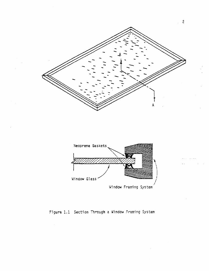
1.1 Section Through a Window Framing System •.••.•.•.•..... 2
1.2 Schematic Representation of Assumed In-PlaneDefonnati ons Along the Edges of the Pl ate •.•..•.••••.. 4:
2.1 Coordinates of Flat Rectangular Plate andNotations of Displacement Components ••.•••••.•..•••... 13
2.2 Section of a Plate Before and After Defonnation •..•.•. 14
2.3 Angular Distortion 15
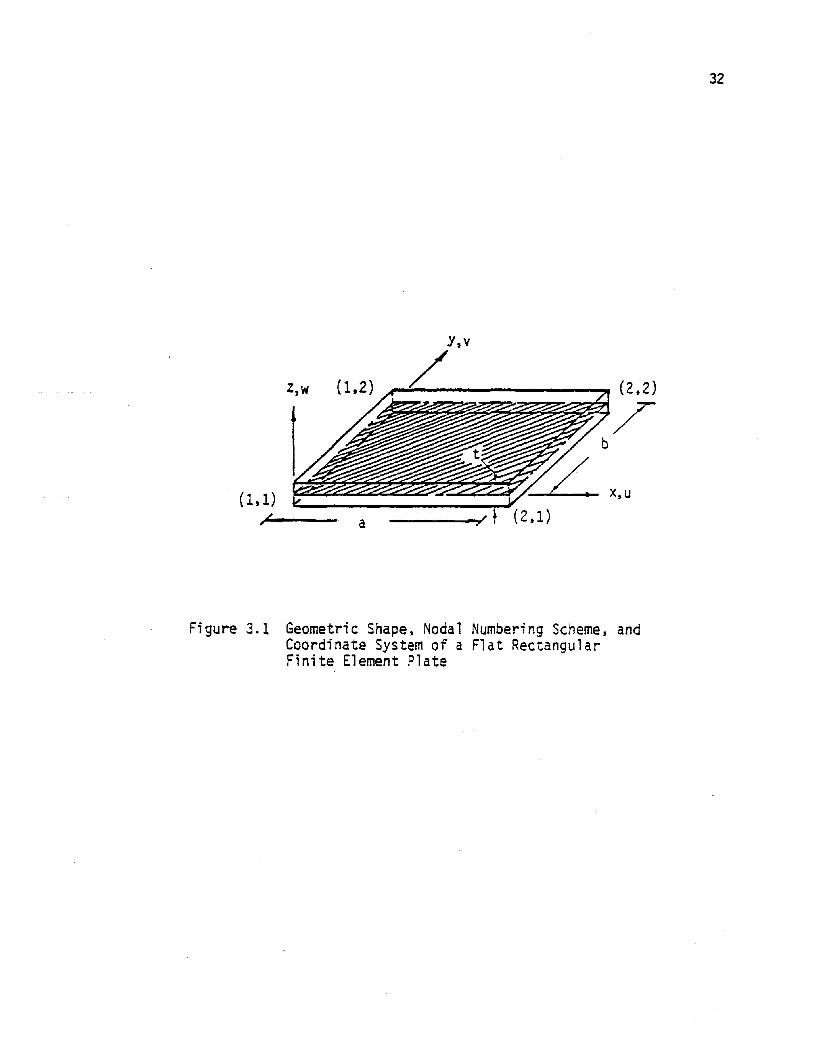
3.1 Geometric Shape, Nodal Numbering Scheme, andCoordinate System of a Flat Rectangular FiniteEl ement Pl ate ..••.•.••..•..•...•.•...•......••.......• 32
3.2 Hermitian Polynomials of Order One.................... 34
3.3 Combined Bending and Membrane Stresses ....•••......... 55
4.1 Incremental Approach.................................. 64
5.1 Load-Deflection of Simply Supported Square Plate:Edge Displacement = 0 68
5.2 Bending Stresses at Center and Corner of SimplySupported Square Plate: Edge Displacement =0........ 69
5.3 Membrane Stresses at Center, Center Edge, and Cornerof Simply Supported Square Pl ate: "EdgeDi splacement = a . . . . . . . . . . . . . . . . . . . . . . . . . . .. . . . . . . . . . . 71
5.4 Load-Deflection of Simply Supported RectangularPlate: "Edge Displacement = a 73
5.5 Bending Stresses at Center and Corner of SimplySupported Rectangular Plate: Edge Displacement =a 74
5.6 Membrane Stresses at Center, Center Edge and Cornerof Simply Supported Square Plate: EdgeDisplacement = a • .•••••.•••..••.•.. .• .••. ••••••.•••••. 76
5.7 Effect of Boundary Edge Condition on Center Deflec-tion of Simply Supported Square Plate..... 78
ix

-Figure
5.8 Load-Deflection of Simply Supported Square Plate:Edge Displacement:; 0 e· •••••••
5.9 Bending and Membrane Stresses at Center of SimplySupported Square Plate: Edge Displacement; a .
79
81
5.10 Effect of Increment Size on Center Deflection ofSimp1y Suppo rted Square P1 ate: EdgeDisplacement; 0....................................... 82
5.11 Effect of Increment Size on Bending Stresses atCenter and Corner of Simply Supported SquarePlate: Edge Displacement; a 84
5.12 Effect of Increment Size on Membrane Stressesat Center and Center Edge of Simply SupoortedSquare Plate: Edge Displacement; 0·'.................. 8S
5.13 Effect of Discretization on Bending Stresses atCenter of Simply Supported Square Plate:rage Displacement, a 86
5.14 Effect of Discretization on Membrane Stresses atCenter and Center Edge of Simply Supported Plate:Edge Di sp1ac ement , 0 87
5.15 Load-Deflection of Simply Supported RectangularPlate: Edge Displacement, 0... 89
5.16 Bending and Membrane Stresses at Center of SimplySupported Rectangular Plate: Edge Displacement, a . .. 91
x

Table
3.1
A.l
A.2
A.3
A.4
A.S
A.6
A.7
A.8
A.9
A.IO
A.ll
A.12
LIST OF TABLES
Equivalent Loads of Uniformly Distributed Lateral Load for aRectangul ar Pl ate. . ... . . . .. . . . . . .. . . . . . . .. . . . . . . . . . . . . . . . . . .. 53
Portion of the [6x48] Matrix [Bo] Represented by the [6x12jMatrix [B011J and Associated Noaal Displacement Parameters ... 108
Portion of the [6x48] Matrix [B ] Represented by the [6x12]Matrix (8012] and Associated Noaal Displacement Parameters ... 109
Portion of the [6x48] Matrix [8 ] Represented by the [6x12]Matrix [8022J and Associated Noaal Displacement Parameters ... 110
Portion of the [6x48] Matrix [eQ] Represented by the [6x12]Matrix [8021J and Associated Noaal Displacement Parameters ... 111
Portionrof ~he [2x48] Matrix [G] Represented by the [2xI2]Matri x I.GIIJ .••....•.•.....•.•.• . .......•...•.......•...•.. 112
Porti on of the [2x48] Matri x [G] Represented by the [2xI2]Matrix [G12] ........•••..................................... 112
Portion of the [2x48] Matrix [G] Represented by the [2x12]Matri x [GZ2J .......•..•..................................... 113
Portion of the [2x48] Matrix [G] Represented by the [2x12]Matrix [GZ1] 11-3
Portion of the [6x48] Matrix [B J Represented by the [6x12]Matrix [BlII] and Associated Noaal Displacement Parameters ... 114
Portion ~of the [6x48] Matrix [BJ Represented by the [6x12]Matrix LBl12J and Associated Noaal Displacement Parameters ... 115
Portion of the [6x48] Matrix [B J Represented by the [6x12]Matrix [Bl22] and Associated Nobal Displacement Parameters ... 116
Portion of the [6x48] Matrix [B ] Represented by the [6x12]Matrix [Bl21] and Associated Nobal Displacement Parameters ... 117
xi

A
a
[B JL
[ BJ
b
[ c JD = [Db]
[ Om ]
*[D ]
E
{ f }
G
[ G]
nHmi(X)
[ Ka ][ KLJ[K ~
cr J
[ KT ]
Mx' My' MxyN , Ny' Nx xy
LI ST OF SYMBOLS
Area of element
Plate dimension in the x-direction
A matrix containing the derivatives of the shapefunctions
A matrix which ;s a function of the slopes Wx andwy ' and contains the derivatives of the shape functions
The sum of [ BO ] and [ BL
]
Plate dimension in the y-direction
A [3x2] matrix which contains the slopes Wx and wy
Flexural rigidity of the plate
A [3x3] matrix containing the plate properties usedfor plane stress analysis
A [6xS] matrix containing [Om J and [Db JYoung1s modulus of elasticity
Force vector
Shear modulus
Amatrix that contains the derivatives of the shapefunctions associated with the slopes Wx and wy
A Hermitian polynomial of order n in the x-direction
The linear stiffness matrix
The "displacmentU stiffness matrix
The lIinitial stress ll stiffness matrix
The total or "tangential" stiffness matrix
Stress moments in plate theory
Stress resultan~s in plate theoryxii

N
{ q }
{ Aq }
t
U
UbUm
u
V
v
w
x,y,z
[ Ct }•
{ ACt }
Yxy
c· .1J
€ij
{ E: }
{ e:L
}
{ e:NL
}
=-m e:m-x' Y'
e:b e: bx' Y'{ 6 }
Assumed shape functions
Load vector
Incrmental load vector
Plate thickness
Strain energy functional
Bending strain energy functional
Membrane strain energy functional
Displacement component in the x-direction
An energy functional
Displacement component in the y-direction
Displacement component in the z-direction
Coordinates of a point within the plate
A vector matrix containing the nodal displacementparameters
A vector matrix containing incremental nodaldisplacement parameters
Shear strain
Kronecker Delta
Strain tensor
Vector of components of the strain tensor
Vector of the linear components of the strain
Vector of the non-linear components of the strain
Components of the membrane strain
Components of the bending strain
A vector matrix containing the slopes Wx and wy
Lame~ parameterxiii
'J
°ij
{ ° }
m m mOX' 0y' °xyb b b
OX' 0y' °xy~(Cl)
Poisson's ratio
Stress tensor
Vector of components of the stress tensor
Components of the membrane stress
Components of the bending stress
Potential energy functional
xiv

CHAPTER 1
INTRODUCTl ON
1.1 Initiation of the Problem
The Institute for Disaster Research at Texas Tech University, acting
in cooperation with other organized research institutes and researchers in
the glass industry, has called attention to the need for a reevaluation of
the window glass design process. Included as a part of this reevaluation
is a study of the response of window glass to wind loads. Structural
modeling of the response of glass plates subjected to lateral loads repre
sentative of wind pressures is a principal concern (6)*.
When glass plates are used in windows and exterior walls of modern
high rise buildings, they are often secured in the framing system by neoprene
gaskets as shown in Fig. 1.1 (2). The response of such glass plates when
subjected to moderately high wind loads (which can be assumed for stress
analysis purposes to be uniformly distributed static loads) is such that
large deflections are experienced. The effects of relatively high loads
combined with uncertainties regarding degrees of fixity of the plate edges
on the response of the glass plate present to the designer a unique large
deflection plate problem.
1.2 Definition of the Problem
The glass plate problem investigated in this research can be modeled
structurally as a simply supported rectangular plate** subjected to moderately
*References used in this report are listed alphabetically by author.
**The terms "glass plate" and II plate ll are used interchangeably to refer tothe glass panel problem investigated in this research.
-...... ............... .....- -'- ---.-
2
---l--- -.-- - -'""~ --... " ---- - "
-- -- -- -- -... -- -- -- --
-
A
Neoprene Gaskets
Window Framing System
Figure 1.1 Section Through a Window Framing System
3
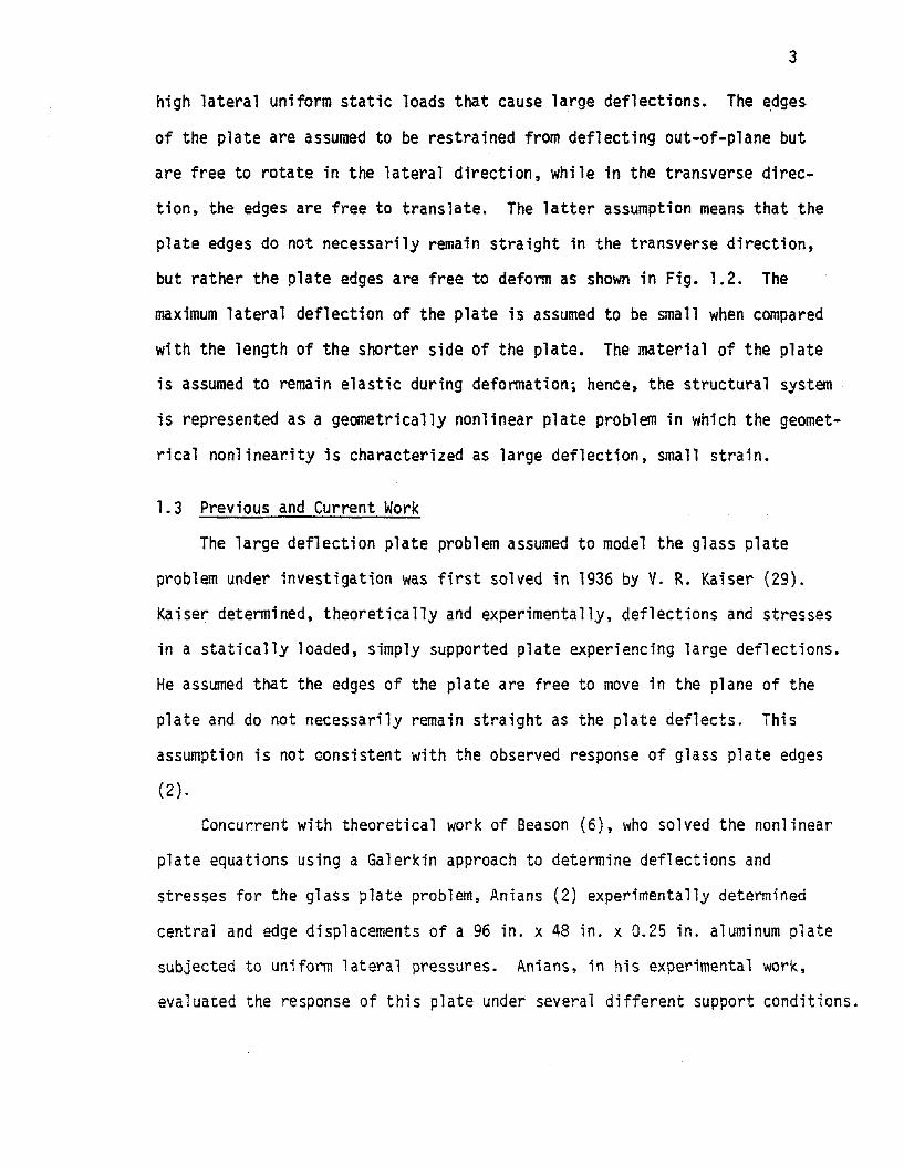
high lateral uniform static loads that cause large deflections. The edges
of the plate are assumed to be restrained from deflecting out-of-p1ane but
are free to rotate in the lateral direction, while in the transverse direc
tion, the edges are free to translate. The latter assumption means that the
plate edges do not necessarily remain straight in the transverse direction,
but rather the plate edges are free to deform as shown in Fig. 1.2. The
maximum lateral deflection of the plate is assumed to be small when compared
with the length of the shorter side of the plate. The material of the plate
is assumed to remain elastic during deformation; hence, the structural system
is represented as a geometrically nonlinear plate problem in which the geomet
rical nonlinearity is characterized as large deflection, small strain.
1.3 Previous and Current Work
The large deflection plate problem assumed to model the glass plate
problem under investigation was first solved in 1936 by V. R. Kaiser (29).
Kaiser determined, theoretically and experimentally, deflections and stresses
in a statically loaded, simply supported plate experiencing large deflections.
He assumed that the edges of the plate are free to move in the plane of the
plate and do not necessarily remain straight as the plate deflects. This
assumption is not consistent with the observed response of glass plate edges
(2) .
Concurrent with theoretical work of Beason (6), who solved the nonlinear
plate equations using a Galerkin approach to determine deflections and
stresses for the glass plate problem, Anians (2) experimentally determined
central and edge displacements of a 96 in. x 48 in. x 0.25 in. aluminum plate
subjected to uniform lateral pressures. Anians, in his experimental work,
evaluated the response of this plate under several different support conditions.

b
T r-'" "'--.- ~ - ....1 ... ......-r~ .... -- ...- tI II I! J, 1\ I\ J\ 1\ I\ I\ I\ lI rI (I 'I I II II 1I ,J I
I '1 l
A I ' A
t I \UY---+-i-' - - - - 1oil \
I ,
r \L ... .-'- ...... --- -- - -- - ~ ....--.. ........-...l_..... -- - ------ -- ---
x
4
I · a -I
~<_ _=M----------- ~Section A-A
Figure 1.2 Schematic Representation of Assumed In-plane Deformations Along the Edges of the Plate
5
This work was conducted in the Civil Engineering Laboratories at Texas Tech
University, Lubbock, Texas, under the supervision of the Institute for
Disaster Reserach, also at Texas Tech University.
Research on the glass plate problem is being continued by researchers
at the Institute for Disaster Research to determine experimentally the
distribution of stresses in uniformly loaded rectangular plates which
experience large displacements.
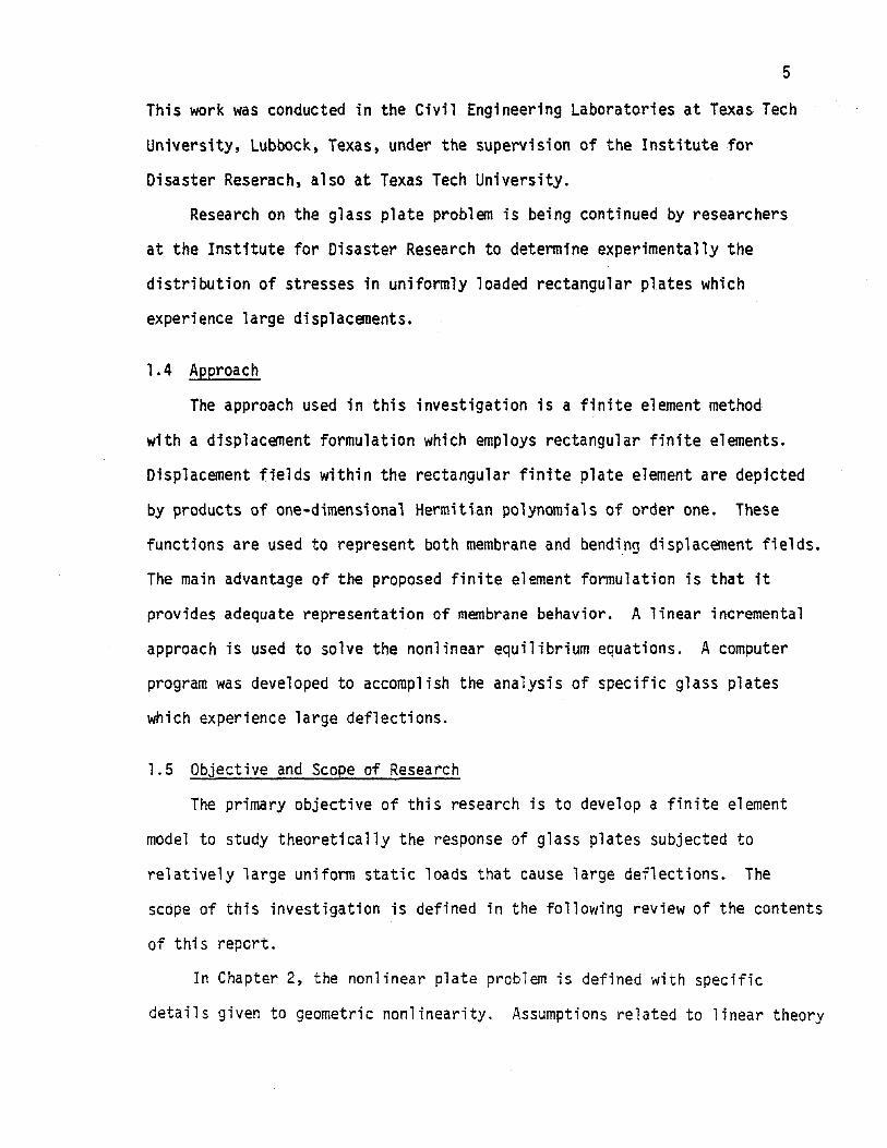
1. 4 Approach
The approach used in this investigation is a finite element method
with a displacement formulation which employs rectangular finite elements.
Displacement fields within the rectangular finite plate element are depicted
by products of one-dimensional Hermitian polynomials of order one. These
functions are used to represent both membrane and bending displacement fields.
The main advantage of the proposed finite element formulation is that it
provides adequate representation of membrane behavior. A linear incremental
approach is used to solve the nonlinear equilibrium equations. A computer
program was developed to accomplish the analysis of specific glass plates
which experience large deflections.
1.5 Objective and Scope of Research
The primary objective of this research is to develop a finite element
model to study theoretically the response of glass plates subjected to
relatively large uniform static loads that cause large deflections. The
scope of this investigation is defined in the following review of the contents
of this report.
In Chapter 2, the nonlinear plate problem is defined with specific
details given to geometric nonlinearity. Assumptions related to linear theory

6
of plates are outlined to introduce the concept of nonlinear plate formu
lation. The nonlinear equilibrium equations are derived in terms of the
displacement components of the plate using an energy approach. Equilibrium
equations thus obtained are converted to the commonly known von Karman
plate equations. Chapter 2 concludes with a brief account of previous
attempts made to solve the nonlinear plate equations.
The first section in Chapter 3 describes the concept of the finite
element method and the second section introduces the rectangular finite
element used to discretize the glass plate. Next, the shape functions
assumed to depict the element displacement fields are defined. This step
is followed by a section in which procedures for deriving the element
linear and nonlinear stiffness matrices are given. Subsequent to the proce
dure for evaluating the equivalent load vector, a-section describing the
calculation of bending and membrane stresses and their combined effects
closes the chapter.
The solution procedure for solving the system of nonlinear equilibrium
equations is presented in Chapter 4 in an incremental form. Also, the
algorithm of the incremental approach adopted in the proposed finite element
formulation ;s given.
Chapter 5 is divided into three sections. In sections 5.1 and 5.2,
examples of uniformly loaded simply supported plates with different in-plane
boundary conditions are solved and results of displacements and stressed are
compared with theoretical and experimental results. The bending and the
membrane stresses are compared separately so that the membrane behavior in
the glass plate can be better assessed. These results are then discussed
in section 5.3. In this chapter, numerical studies conducted on the glass
plate problem reveal that the convergence of stresses differs between

7
bending and membrane stresses, and depends upon the fineness of the finite
element discretization, the location within the plate and the relative
magnitude of the loading increment. This observation, in the author's
opinion, is valuable for anyone involved in analyzing geometrically nonlinear
plate problems.
In Chapter 6, conclusions are offered and recommendations for further
investigation are advanced.

CHAPTER 2
LARGE DEFLECTION THEORY OF THIN PLATES
2.1 Nonlinear Plate Problems
In linear analysis of thin plates by the classical theory,
it is assumed that the middle surface of the plate is free from
deformation. This assumption is valid only if the plate is bent
into a developable surface (63); a developable surface is one
that can be made from a flat sheet without causing any in-plane
strain of the middle surface: i.e., a cone or an open ended cy
linder. However, application of the classical theory to problems
in which the middle surface of the plate experiences some straining
will still be valid depending upon the kind of restraints imposed at
the edges and the magnitude of maximum lateral displacement of the
plate. For example, if the lateral displacement of a uniformly
loaded clamped plate is small in comparison with its thickness, itI
is found that the calculated stresses of the middle surface, which
in pl ate theory are call ed the membrane stresses, are sma 11 and of
negligible value when compared with the bending stresses (61). The
membrane stresses are also found to be small in the case of cylindri-
cal bending of uniformly loaded long rectangular plates with edges
that are free to move in the plane of the plate even though maximum
displacements in such plates are of the order of the plate thickness.
However, if the edges of these plates are restrained from moving,
the membrane stresses become significant and, hence, stress distri-
butions obtained by the classical theory will be in error (65).
Therefore, wnen the membrane stresses become large and the deflec-
8
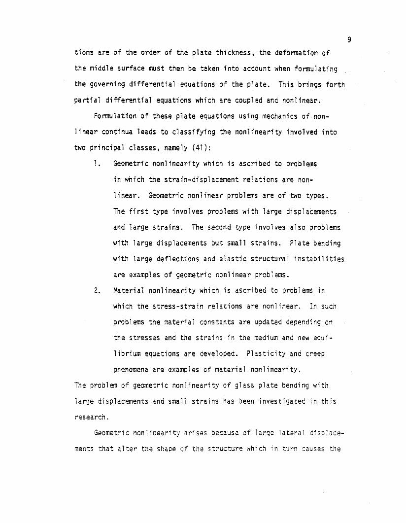
tions are of the order of the plate thickness, the deformation of
the middle surface must then be taken into account when formulating
the governing differential equations of the plate. This brings forth
partial differential equations which are coupled and nonlinear.
Formulation of these plate equations using mechanics of non
linear continua leads to classifying the nonlinearity involved into
two principal classes, namely (41):
1. Geometric nonlinearity which is ascribed to problems
in which the strain-displacement relations are non-
linear. Geometric nonlinear problems are of two types.
The first type involves problems with large displacements
and large strains. The second type involves also problems
with large displacements but small strains. Plate bending
with large deflections and elastic structural instabilities
are examples of geometric nonlinear problems.
2. Material nonlinearity which is ascribed to problems in
which the stress-strain relations are nonlinear. In such
problems the material constants are updated depending on
the stresses and the strains in the medium and new equi
librium equations are developed. Plasticity and creep
phenomena are examples of material nonlinearity.
The problem of geometric nonlinearity of glass plate bending with
large displacements and small strains has been investigated in this
research.
Geometric nonlinearity arises because of large lateral displace
ments that alter the shape of the structure which in turn causes the
9

10
applied loads to change their distribution (41). This nonlinearity
can be introduced into the formulation of the system equations either
by inclusion of high powers of the derivatives of the displacements
or their products in the strain-displacement relations or by coordi
nate transformations in which the coordinates of the system account
for all nonlinear geometric effects (69).
In order to derive the nonlinear thin plate equations, it is
worthwhile to examine the assumptions limiting the linear theory of
thin plates.
2.2 Assumptions of the Linear Theory of Thin Plates
The classical theory of thin plates assumes that (21, 61):
1. The plate is initially flat and free from stresses,
2. Tractions on planes parallel to the middle surface are
small and can be neglected, and strains vary linearly
within the plate thickness,
3. The thickness, t, is much smaller than the typical plate
dimension, a, where a is the shorter side in the case of
a rectangular plate,
4. The maximum deflection of the middle surface of the plate
in the lateral direction is small in comparison with the
thi ckness,
S. The middle surface of the plate is free from deformation
duri ng bendi ng,
6. The slopes of the deflected middle surface are small com
pared to unity, and

7. The vertical deflection of a point on the middle surface
of the plate is measured on a normal to its initial plane.
These are generally known as Kirchoff's assumptions in plate theory.
If these assumptions are considered, all stress components can be
calculated in terms of the normal deflection of the middle surface
of the plate, w, which is a function of two coordinates in the plane
~f the plate (68).
2.3 Nonlinear Thin Plate Equations
If assumptions 4 and 5 above are violated, the middle surface
of the plate will experience some deformation which must be taken into
consideration when deriving the differential plate equations. The
equations thus obtained are nonlinear and the solution becomes much
more complicated (61). In 1910, Theodore von Karman derived the non-
linear plate equations and suggested that the quadratic terms in Wxand wy* which are the derivatives of the lateral displacement w, with
respect to the x and y directions, respectively, be retained in the
strain tensor but that other quadratic terms involving higher powers
of the derivatives of the in-plane displacement components u and v be
dropped because they have about the same magnitude as the square of
the-strain components. With this suggestion and in addition to the
assumptions used in the classical theory of thin plates, excluding
assumption 4~ von Karman assumed that (21):
1. The magnitude of the lateral deflection w is of the
same order as the plate thickness, but small when compared
*Subscripts on symbols denote derivatives with respect to that subscript unless stated differently.
11,

12
with the typical plate dimension a, where a is the shorter
side in the case of a rectangular plate, i.e., Iwl =Q(t)*,
w«a.
2. The in-plane displacement components u and v are small and
hence higher powers of their derivatives and their products
are negligible.
For rectangular plates, the use of a Cartesian coordinate system
is the most convenient (Fig. 2.l). Consider a flat rectangular thin
plate;n a right-handed rectangular Cartesian frame of reference with
the x-y plane coinciding with the middle surface of the plate in its
initial undeformed state, and the z-axis perpendicular to it as shown
in Fig. 2.1. Let the displacement components of an arbitrary point
(x, y, z) be denoted by (u, Y, w) and those of the corresponding
point (x, y, O) of the middle surface be denoted by (u, Y, w).
Using assumptions 5 and 6 introduced in the'previous section, and
considering the geometry of a section of the plate at y = constant,
as shown in Fig. 2.2, and by comparing the section before and after
it is deflected, the displacement component u can be written as
similarly,
-u = -z VIX
(2. 1)
-v = -z '1-'y (2.2)
By comparing the rectangular parallelogram abcd shown in Fig. 2.3
which is located at a distance z from the middle surface, with its
*O(t) stands for a function of the order of t.

Tt
1.
z y
13
Middle Surface
Figure 2.1 Coordinates of Flat Rectangular Plate and Notationsof Displacement Components

14
z,w
II 1 2
I y=constant
X,u•
Undeformed Section
2
1 '
1 '
I
I
Ll-~ x---""",-dx
1
Figure 2.2 Section of a Plate Before and After Deformation

15
y,v
x, u·
u
d l
C I _---"7~ / /ay /c d r--// b l
t I_-r --t dy
a Idx ail .
tv
~ z=constant+ .:l dx b I
II
Q
- + au ~
_ ailv + ax
Figure 2.3 Angular Distortion
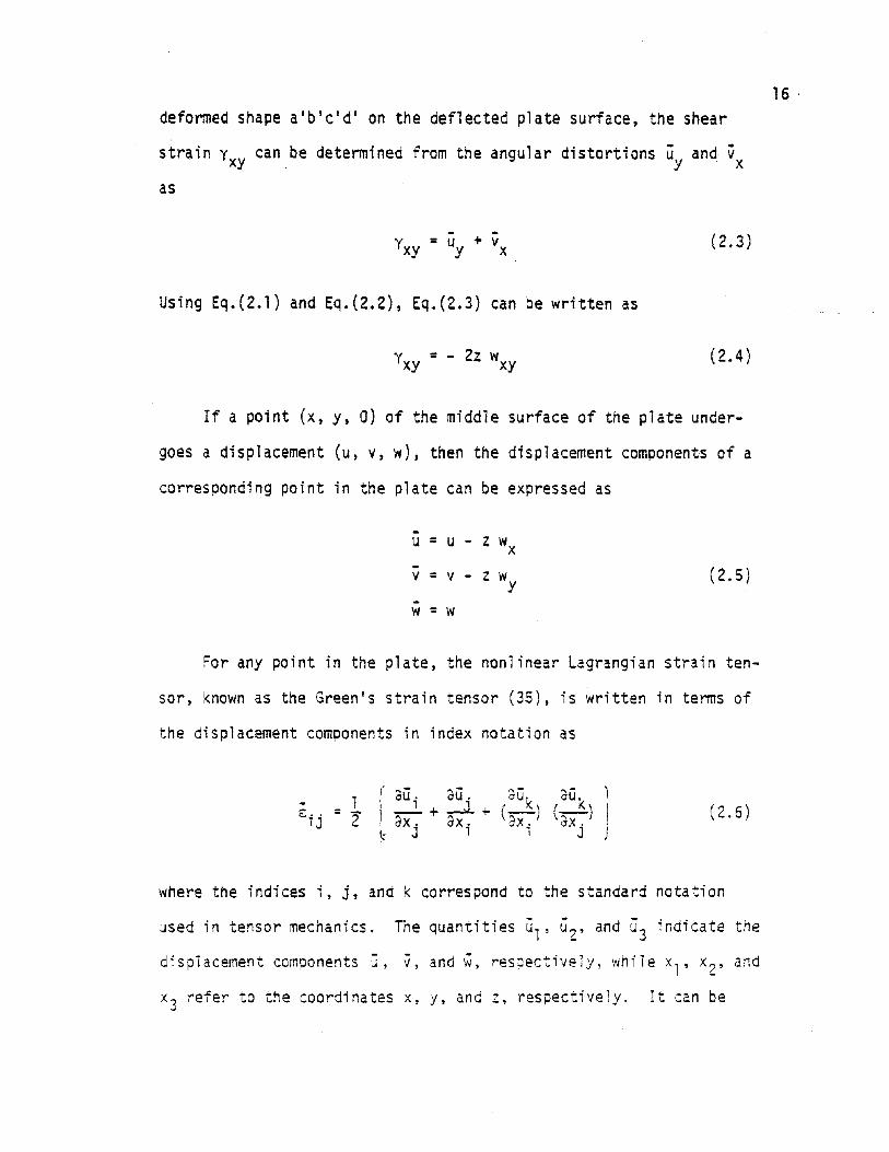
deformed shape a1b'c'd ' on the deflected plate surface, the shear
strain Yxy can be determined from the angular distortions Uy and Vxas
16 .
- + vYxy = uy x
Using Eq.(2.1) and Eq.(2.2), Eq.(2.3) can be written as
y = - 2z wxy xy
(2.3)
(2.4)
If a point (x, y, 0) of the middle surface of the plate under
goes a displacement (u, v, w), then the displacement components of a
corresponding point in the plate can be expressed as
-u = u - z Wx- (2.5)v = v z wy-w = w
For any point in the plate, the nonlinear Lagrangian strain ten
sor, known as the Green's strain tensor (35), is written in terms of
the displacement components in index notation as
(2.6)
where the indices i, j, and k correspond to the standard notation
used in tensor mechanics. The quantities u" u2' and u3 indicate the
displacement components u, ii, and w, respectively, whi1e xl' x2' and
x3 refer to the coordinates x, y, and z, respectively. It can be

17
shown that Eq. (2.6) can be reduced to a simpler form, if assumption 2
introduced in section 2.2 and von Karman's assumption are considered.
Assumption 2 implies that szx =Syz =Sz =O. These relations signify
the fact that points on the plate which are initially on a normal to
the middle surface before deformation remain on the normal to the mid-
d1e surface after deformation; this is known as the IIKirchhoff assump-
tion ll in the theory of plates. And von Karman's assumption suggests
discarding all quadratic terms in Eq.(2.6) except w~, w~, and wxwy.
Hence, Eq.(2.6) can be written as
- - + 1 WZSx = Ux 2 x
- - 1 20 (2.7)Sy = v + - wy 2 y
- u + v + w wYxy =Y x x Y
Using Eq.(2.5), Eq.(2.7) can be expressed in terms of the middle sur-
face strains EX' Sy' and Yxy as
-ex = .- - zw-x xx
- (2.3)Ey = Sy - ZINyy
- 2zwxyYxy = Yxy -
where
1EX = U + - 'liZ
X 2 x
Sy = v + 1 V'I 2 ( 2.9 )y 2 y
Yxy = u + v + W INY X X Y
Corresponding to Green's strain tensor, the Kirchhoff's stress
tensor in the Lagrangian description is expressed in index notation
for an isotropic homogeneous material as (21)
18
(2.10)
where
2GvA = (l-2v)
and
EG = 2(l+v)
where A and G are the well-known Lame parameters. The indices i, j,
and k in Eq.(2.10) correspond to the conventional mechanics notation,
and Qij denotes the Kronecker delta. The Young's modulus of elasti
city and the Poisson's ratio of the material are indicated by E and
v, respectively. Based on the Kirchhoff's assumption of plate theory
the Kirchhoff's stress tensor can be reduced to
- _ E (~ + \) Ey )O'x - r:vz- <:Ox
- E - + v : ) (2. 11 )O'y = 1-v2 (s.y <:Ox
- E -O'xy = 2( l+v) Yxy
where cr x' cry' and crXy are the stress components at any point in the
plate. Inversion of Eq.(2.11) yields

crxy
- 1 (- - )c; =- cr -vcrx E x y
€ = 1 (0 - v 0 )y E y x
2(1+v)YXy = E
(2.12)
19
Eq.(2.11) expresses a state of plane stress for which the strain
energy density is written as
(2.13)
The strain energy of the entire plate is the volume integral of Eq.
(2.13) which can be written as
or
(f (+t/2
U = J {I Uo dz }dx dy) -t/2
(2.14)
(2.15)
Substituting Eq.(2.8) into Eq.(2.13) and then substituting the
resulting expression in Eq.(2.15), the strain energy U, when inte-
grated over the thicKness t of the plate, separates into a sum U =
Um + Ub, where Um is the membrane strain energy which is linear in
t, and Ub is the bending strain energy which is cubic in t. If the
material properties E and \) are considered constant, U and Ub canm
be written as

and
20
(2.16)
+ W2 + 2v w w + -21 (1-v) W
X2yJ dx dyyy xx yy
(2.17)
The potential energy function of a uniformly distributed load
q (x, y) applied to the plate is defined as
v =- ff w q(x,y) dx dy (2.18)
The total potential energy ~ of the plate is the sum of the
strain energy U and the potential energy function V, that is
(2.19)
Using Eu1er l s equation of the calculus of variations (32), it can be
demonstrated that the differential equations of equilibrium in terms
of the middle surface displacement components (u, v, w) in the x, y,
and z directions are obtained from the total energy expression of Eq.
(2.19) and they are written as
" 1 0 V 2 1-v Q [ 1o [+ • w. l' + v + W 1," = 0- u v v '-2 wx ' - 'II - - - u •~x x y 2 y.' 2 ;y y x x y~(2.20 )
3 [ ,1 2 \) 2" 1-I) or,v + v u ,. -2 wy + - w J + - - U ,.ay y x 2 x 2 oX ~ y v +W\'IJ=ox x y(2.21 )
w + 2w + w =S. + 12xxxx xxyy yyyy 0 tT
r-
{( U + -21 w2.) +x X
L
21
w +l-v (u + v + w w ) w ]yy y x x y xy
where
The quantity 0 is calied the "flexural r;gidityll of the plate.
(2.22)
Eq.(2.20) through (2.22) are the basic equilibrium equations for
the geometric nonlinear problem in a displacement formulation. Alter
natively, these equations can be converted to the well-known von Karman
plate equations if the membrane stress resultants defined in plate
theory by the statical relations (21)
=ft
/2o
x.
N dzx-t/2
(+t/2N - J Oy
dz (2.23)Y
-t/2
r+ t / 2N = ! ':Jxy dz,
xy II
I-' -t/2
are expressed in terms of a stress function F(x, y) such that
Using Eqs.(2.9) and (2."), it can be demonstrated that
N = ,·Etz (s + v E: )X -v x y
(2.24)
22
From Eqs.(2.24) and (2.25),we can write
aZF(x,y) = Fxx =~ (E: + V € )ax z -v y x
a2F(x,y) = F = l:~Z (E:x + v Sy)ayz yy
aZF(x,y) F Et= xy = - 2(1+v) ~xyaxay
From Eqs.(2.20), (2.21), (2.22), and (2.25), we get
3N aN_.2. + --Ei.. = 0ax ay
(2.25)
(2.26)
(2.27)

23
(2.28)
o [w + 2w + w ] = q + N wxx + 2N w + rJ wxxxx xxyy yyyy x xy xy y yy
(2.29)
Substituting Eq.(2.2S) in Eq.(2.29), we get
o [w + 2w + w ] = q + F w - 2F w + F wxxxx xxyy yyyy yy xx xy xy xx yy
(2.30)
A second relation between the functions F(x, y) and w(x, y) can
be obtained by deriving the strain compatibility equation. If Eq. (2.25)
is inverted, it yields
_ 1 (Fxx)E:x - IT Fyy - v
=-' (F - v Fyy) (2.31 )E:y Et xx
y =- 2( l+v) Fxy Et xy
Using Eq.(2.9), it can be shown that the compatibility condition
can be obtained as
Substituting Eq.(2.31) in Eq.(2.32), we get
F + 2F ~ F = Et rw 2 - w w 1xxxx xxyy yyyy - xy xx yy~
(2.32)
(2.33 )

24
Eq.(2.30) and Eq.(2.33) are the well-known von Karman equations. This
form of the nonlinear plate equations is most known to investigators
dealing with nonlinear plate equations. The von Karman equations are
mixed equations which involve a stress function and a displacement•
function. Such equations are not treated by the displacement approach
in the finite element method which is used in this report.
For more understanding of the formulation of the nonlinear plate
equations, the interested reader is advi·sed to consult the following
references (21,32, 35, 50, 60,61, 62,63, 64, 65).
2.4 Brief Review of Previous Wor~
on Solution of Nonlinear PlateEquations
To the best of the writer's knowledge, there is only one original
closed form solution of the von Karman nonlinear thin plate equations.
This solution is attributed to Samuel Levy (33, 34) who repre-
sented the nonlinear differential equations in terms of trigonometric
series and solved for the deflections and the stresses in clamped and
simply supported uniformly loaded rectangular plates. Levy solved two
types of simply supported uniformly loaded rectangular plates: one,
the boundaries of which remained straight and were immovable (he
called that type of boundaries "Edge Displacement = a"), and two,
the boundaries of which are assumed to remain straight and free to
move in the in-plane direction of the plate (he called that type of
boundari es "Edge Compress ion = 0") (33, 34).
Because of the difficulties involved in solving the von Karman
nonlinear thin plate equations, researchers directed their efforts
to the development of alternative approaches to the problem which
are based on either simplified physical theories or approximate

25
numerical methods such as the variational methods, the finite differ
ence method, and the finite element method (60).
Marguerre, K., Bengston, H. W., Timoshenko, 5., Cox, H. L., and
von Karman are some of the early pioneers who formulated approximate
solutions based on simplified physical theories to solve the nonlinear
thin plate equations. According to Timoshenko, numerical results ob
tained by these approximate methods give satisfactory accuracy for
technical purposes. However, he cautioned that a good understanding
of the hypothesis providing the basis of the method is essential in
the application of these approximate methods (7, 8, 13, 63, 65).
In 1936, Kaiser, R., solved the nonlinear thin plate equations
using finite difference formulations. In his solution, Kaiser as
sumed that the boundaries of the plate were free to move in the in
plane direction of the plate and that the edges did not necessarily
remain straight. Kaiser supported his theoretical work with experi
mental results that he obtained from a 60cm x 60cm x O.3l5cm uniformly
loaded simply supported square plate and showed very good agreement
of his theoretical and experimental works (29). Also, in 1948,
Wang, C. T., used the finite difference method to solve nonlinear
problems of uniformly loaded simply supported rectangular plates with
boundary conditions that approximate plates with riveted edges. Wang
used the successive approximation and the relaxation methods to solve
his finite difference equations. The numerical results Wang obtained
by his formulation do not agree with those obtained by Levy (70, 71).
With the fast and advanced development of computers the finite
element method placed in the hands of researchers an alternative ver-

satile tool for tackling the large deflection plate problem. The
finite element method does not directly de~l with p~rtial differ
ential equations of equilibrium or compatibility; rather, it con
verts the problem into one requiring the solution of simultaneous
equations. Advancement of this field in solving the nonlinear
plate equations is briefly outlined in the next chapter.
26

CHAPTER 3
THE FINITE ELEMENT METHOD
3. 1 Concept
Very often, the structural engineer is confronted with the prob
lem of determining stresses and displacements in continuous structural
systems which have complicated configurations and which cannot be
handled by available classical methods of stress analysis. A numeri
cal discretization technique, so called "finite element method,1I
enabled the structural engineer to tackle such problems using elec
tronic computers. The concept of this method is simple: if the be
havior of a subregion or a finite part, which is known as IIfinite
element,1I of the whole structural system can be modeled, then the be
havior of the entire structural system can be modeled as well. In
this case, the entire structural system is considered to be made-up
of an assemblage of finite elem~nts which are interconnected at
joints called llnodes" or II nodal points. II Based on this concept,
users of the finite element method are able to divide a structure
into several substructures which are made of rather simple geome
tric shapes such as bars, beams, triangles, rectangles, tetrahedra,
and prisms. These different shape elements or a combination of
them make it possible to model any structure of any arbitrary shape.
Since 1960, the finite element method has gained increasing popu
larity among structural engineers. This is attr~buted to the fact
that the method handles easily not only problems having complex
geometry and mixed boundary conditions, but also problems having
nonlinear characteristics.
27

28
Formulation of the equations of the finite element model is
based upon energy. principles. Either of the two well-known methods
of structural analysis, namely the force or displacement method,
can be used to derive the equations necessary for the finite element
analysis. In finite element applications, the displacement model
has been employed most commonly. This is because a displacement
model can be expressed in various simple forms such as polynomials
and trigonometric functions, whereas such functions in the force
model are relatively difficult to formulate. Also, the displace
ment model has better computational schemes for most problems in
solid mechanics (19).
The finite element method can be viewed as an extension of
the Ritz method, in which the displacement of a continuum are ap
proximated by a set of assumed functions. The unknown constants in
these functions are detennined using the well-known minimum poten-
tial energy theorem which states that (17):
llAAlong all displacement configurations that satisfy internalcompatibility and kinematic boundary conditions, those thatalso satisfy the equations of equilibrium make the potentialenergy a stationary value. If the stationary value is aminimum, the equilibrium is stable. 1I
While in the classical Ritz method, the assumed displacement func
tion describes the total displacement field of the entire continuum;
in the finite element, displacement functions are assumed for each
element and the entire displacement field of the continuum is approxi
mately expressed in terms of their nodal point values. The total po-
tential energy of individual elements has a stationary value when the
whole system is in equilibrium. This condition leads to the minimi-

29
zation of the total potential energy function of the whole assemblage
of elements, which in turn yields the necessary equations correspond
ing to its equilibrium state (17). The resulting set of equations ;s
called the "stiffness matrix" equation.
The basis for the formulation of the stiffness matrix equations
is fully explained in numerous publications by authors such as Argy
ris (3), Martin (40, 41), Gallagher (22), Zienkiewicz (73)t Cook (17},
Desai (19), and many others. Hence, only the essential features of
the displacement approach of the finite element method pertinent to
the problem under investigation are described in this report.
For accomplishing a finite element displacement analysis, the
following steps must be considered:
1. Discretization of the structure into some convenient geo
metrical shapes to model t~e overall geometry of an actual
structure.
2. Selection of a displacement field that belongs to a finite
class or space of functions continuous in the domain of
the selected element and satisfies requirements of rigid
body motion, constant strain, and a minimum number of
conditions of displacement continuity along its boundaries.
3. Derivation of the element stiffness matrix which ;s a
function of the geometric and constitutive properties of
the element by relating generalized displacements and
their associated generalized forces.
4. Formation of the global stiffness matrix by assembl ing the in
dividual element stiffness matrices to a common system of

reference called the global system. The resulting global
matrix equation expresses the equilibrium state of the
entire structure.
5. Solution for nodal displacements after prescribing the
boundary conditions on the structure.
6. Determination of the strains which are related to the
displacements. The stresses are then calculated using
Hooke1s law.
3.2 Rectangular Finite Element·
To represent the complex geometric nonlinear behavior of the
glass plate problem under investigation, it was decided to provide
adequate representation of the membrane behavior of the structure
that is comparable to the bending. This is accomplished by using
displacement shape functions suggested by Bogner, Fox, and Schmit
(9) which are limited to elements with boundaries parallel to an
orthogonal coordinate system. A rectangular plate element due to
SChmit, Bogner, and Fox (56) is used in this work as a discretizing
unit. The action of the four corner nodes of this geometrically
nonlinear bending membrane rectangular plate element is represented
by twe Ive degrees of freedom: four degrees of freedom w, \~Jx' Wy'
and wxy to represent the bending action and eight degrees of freedom
u, ux' uy ' u ,v, v , v , and v to represent the membrane action.xy x y xyThese degrees of freedom will be defined in a later section of this
chapter. Twelve degrees of freedom per node result in a 48 degrees
of freedom rectangular finite element. The geometry, the nodal
30

numbering scheme, and local coordinate system for this element are
shown in Fig. 3.1.
The displacement shape functions assumed to represent the dis-
placement components u, v, and w of the middle surface of the plate
element are formulated using products of one-dimensional Hermitian
polynomials of order one. It is noted by Schmit, Bogner, and Fox
(56) that although the use of these interpolation polynomials to
represent the membrane behavior increases the number of degrees of
freedom, it adequately represents the six-rigid body modes and des-
cribes the membrane stress state more accurately.
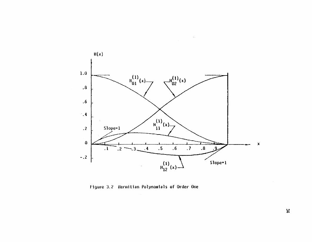
3.3 Hermitian Polynomials
AHermitian polynomial of order n is a polynomial of degree
2n+l and can be written as
31
which gives, when x = x.,
and
k =m
k ~ m
for m= 0 to n
or when x = x.J
(3. 1)
<(1,1)
,
Figure 3.1 Geometric Shape, Nodal Numbering Scheme. andCoordinate System of a Flat RectangularFinite Element Plate
32

33'
By setting n =1 and m=0 and 1, a set of Hermitian polynomials of
order one is obtained. The set is a set of cubics giving shape func
tions for a line element ij at the ends of which slopes and values
of the function are used as variables. Such a set of polynomials
can be written for the rectangular finite element as
For all xO<x<a (3.2)
These are known as the "osculatory polynomials" and are plotted in
Fig. 3.2. Similar expressions for the y-direction are obtained by
replacing x by y and a by b.
Using these Hermitian interpolation formulas, the middle surface
displacement components u, Y, and w of a typical discrete element can
be approximated by a sum of their products and undetermined parameters.
For example, the displacement component u, in a rectangular plate e1e-
ment can be expressed as
u(x ,y)2 2 1(1) (1) (1) (1)
:: i: L: HO' (x)HO' (y)u;. + H" (x)HO' (y)u i' +;=1 j::1 i 1 J J 1 J x J
'-
(1)( ) (1)/ )Ho ' x H,. \y U ..1 J yl J
(3.3)
H(l)( )H(l )(\) ]+ '1' x ,. y u ..1 J XY1J
1.0
.8
.6
.4
.2
o
-.2
H(x)
H(l) (Xl)01 ~)(Xl
(1)H12 (x)
Slope=1
x
Figure 3.2 Hermitian Polynomials of Order One
~

where the indicies (i, j) refer to a node of the element as shown in
Fig.3.1, and the displacement parameters are defined as
35
u· .lJ
= U displacement at node (i) j)
=
=
(~) at node (i, j)
(~) at node (i, j)3y
(~~~y) at node (i, j)
Expressions for the displacement components v and w can be written in
s1milar form as in Eq.(3.3) in which the displacement parameters for
each component are interpreted as shown above.
The displacement components can be written more conveniently in
matrix form as
{~l = {-:} = [N] {al (3.4)
where {~} is a vector matrix representing the displacement compo
nents, [N] is a matrix containing the assumed shape functions which
are dependent on the Cartesian coordinates x and y, and {a} is a
vector containing the nodal displacement parameters.
There are certain requirements and limitations imposed on the
assumed shape functions to guarantee a successful finite element
formulation. Basically, a shape function assumed over the region
of an element is supposed to represent the pattern of displacements
in that element. Therefore, a primary consideration in choosing a

36
shape function is that the function must maintain some minimum con
tinuity requirements between adjacent elements as they deform. The
function must also satisfy certain other requirements to minimize the
discretization errors in the analysis. These requirements, outlined
below, are satisfied for both bending and membrane behavior in this
study. The requirements are (16):
1. The functions must include all rigid body displacement states.
That is, they must be independent of the external reference
system so that the solution to a problem will be invariant
with respect to the position of that external reference sys
tem and hence prevent self-straining of the elements.
2. The functions must include uniform strain states to assure
the convergence of the finite element analysis to the ac
tual strain field as the element size is reduced.
3. The functions and their normal slopes are uniquely specified
along any element interface by nodal values selected on that
interface. In other words, the displacements and their nor
mal derivatives on an interface of an element are dependent
only upon the nodal values occurring at the nodes associated
with that interface. This requirement assures compatibility
and continuity of the assumed shape function.
4. The shape functions must be linear functions of the nodal
parameters so that the resulting system equations are a set
of simultaneous, linear algebraic equations in terms of
these parameters (44).
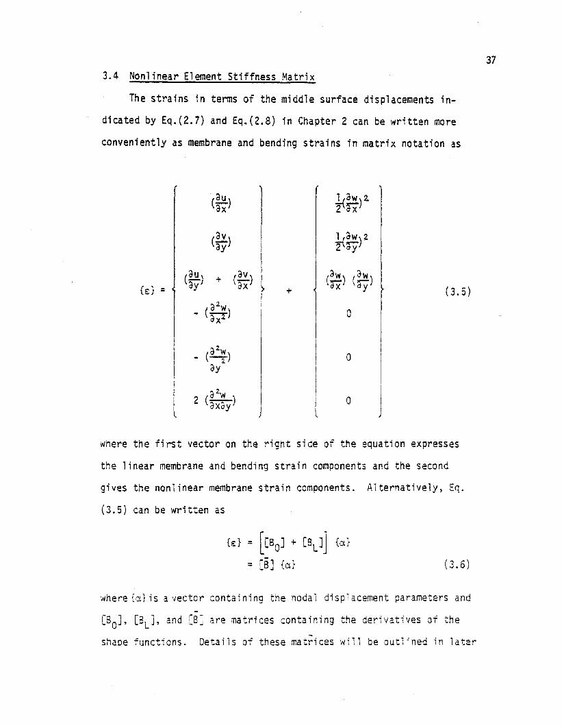
3.4 Nonlinear Element Stiffness Matrix
The strains in terms of the middle surface displacements in
dicated by Eq.(2.7) and Eq.(2.8) in Chapter 2 can be written more
conveniently as membrane and bending strains in matrix notation as
37
(~)ax
(~)ay
(au \ + (~){e:} = ayl ax +
a2w- (-)ax2
_ (a2~)
ay
2 a2w(hay)
(3.5)
o
o
o J
where the first vector on the right side of the equation expresses
the linear membrane and bending strain components and the second
gives the nonlinear membrane strain components. Alternatively. E~.
(3.5) can be written as
{e:} = [[80J + [BLJ] {cd
= [B] {a} (3.6)
where {cd is a vector containing the nodal displacement parameters and-
[80J. [BLJ. and [BJ are matrices containing the derivatives of the
shape functions. Details of these matrices will be outlined in later

sections of this chapter.
The corresponding "stresses" are in fact the membrane tractions
per unit length in the x and y directions as defined in Eq.(2.23) in
Chapter 2, and the bending and twisting moments per unit length in
the x and y directions as defined in plate theory.
N Ix
Ny
Nxy{cr } = (3.7) .
M"x
M
J
y
Mxy
Because the membrane strains and stresses are assumed to have
constant variations across the thickness of the plate, the membrane
stresses are obtained from the following expressions
Nm xOx = t
Nm -'i.. (3.8)0y = tNm = ...&
°xy t
where om and om refer to the membrane stresses in the x and y direc-x y
tion, respectively, O~y indicates the membrane shear stress, and t
is the thickness of the plate.
The bending strains and stresses are assumed to vary linearly
across the thickness of the plate and they can be found anywhere
38

along the thickness from the following expressions
39
crb 12= f3 Mxzx
crb = 11 M zY t3 Y
b 12crxy = tT MXYZ
(3.9)
where cr~ and cr~ are the true bending stresses in the x and y direc
tions, cr~y is the true bending shear stress, and z is the vertical
distance measured from the middle surface of the plate.
Assuming linear, isotropic, homogeneous material within the
element, the stress-strain relations are expressed as
{cr} = [0*] {e:} (3.10)
where [O*J is a matrix defined in terms of the elastic constants of
the ma teri a1 as
r 1 v 0 0 a a
v 1 0 a 0 0
0 a l-v 0 a 0E -2-[O*J =- t 3 vt 3 (3.11)l-v2-
0 0 0 12 IT 0
0 a a vt 3 t 30IT 12
I
t 3 (1-v)l 0 0 0 a 0 24j
where E is Young1s modulus of elasticity, v is the Poisson1s ratio,
and t is the thickness of the plate.
Using the virtual displacement principle and Eq.(3.4), a virtual
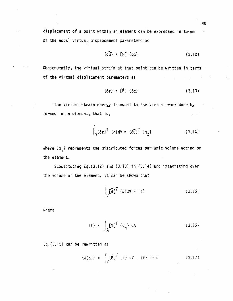
displacement of a point within an element can be expressed in terms
of the nodal virtual displacement parameters as
40
{o7n = [N] {oa.} (3.12)
Consequently, the virtual strain at that point can be written in terms
of the virtual displacement parameters as
{cd = [8] {ca.} (3.13)
The virtual strain energy is equal to the virtual work done by
forces in an element, that is,
(3.14)
where {qz} represents the distributed forces per unit volume acting on
the element.
Substituting Eq.(3.12) and (3.13) in (3.14) and integrating over
the volume of the element, it can be shown that
where
{f}
J{ [B]T {o}dV = {f}
"
= f [N]T {q } dAA n
(3.15)
(3.16)
Eq.(3.15) can be rewritten as
{~(a.)} =( - ~
I [B] I {a} dV - U} = 0J V
(3.17)

41·
where {~(a)} is a function of the nodal displacement parameters a.
Taking the appropriate variations of the function {~(a)} in
Eq.(3.l7) with respect to a, we get
r T J - T{o~(a)} = [SJ {ocr} dV + v[oS] {cr} dV"V
Taking the appropriate variations of Eq.(3.10) yields
{ocr} = [D*J {O€}
Substituting Eq.(3.13) into Eq.(3.19), we get
{ocr} = [O*J [B] {c€}
(3.18)
(3.19)
(3.20)
In Eq.(3.6), [8] = [BOJ + [BlJ, where [Bl ] is a function of the
displacement parameters a, hence by taking the variations of [BJ, we
obtain
[08] = [eEL]
Substituting Eq.(3.20) and (3.21) into Eq.(3. 18), one gets
(3.21)
(3.22)
Expanding the first term in Eq.(3.22) by substituting the value of
[B] given in Eq.(3.6) we get
fVCB]TCO*J[8J dV {cal = [fvCBO]T[O*][BOJ dV +
_ r _ (-
[BOJ1[O*][BL] dV + )1 [BLJ1[O*][BLJ dV + I [8LJ1[O*][BOJ
V V )v
(3 ?"\.4..))
dV] {car

42
The first term on the right side of Eq.(3.23) is the usual linear
stiffness matrix which can be expressed as
(3.24)
The rest of the terms in Eq.(3.23) signify the effects of large dis
placements on the stiffness of the structural system. This may be
expressed as
[~J = Jv[BOJT[O*][BLJ dV + fv[BL]T[O*J[BL] dV +
(3.25)
where [KLJ is called the 1I1 arge displacement ll stiffness matrix (73).
In Eq.(3.22), the second term can be written as equal to [kaJtimes
{Oo.}, where [K ] is called the lI;nitial stress ll or the,lIgeometriclla
stiffness matrix (73) which depends on the stress level in the ele-
ment and which can be shown to be symmetric. That is
(3.26)
Alternatively, Eq.(3.18) is written as
(3.27)
The stiffness matrices [KOJ and [KlJ are calculated by integra
ting the expressions given by (3.24) and (3.25) over the volume of
the element after the matrices [SOJ and C8L] are evaluated. Evalua-

tion of these matrices is outlined in the following two sections
which are followed by a section outlining the procedures involved
in calculating the stiffness matrix [KcrJ.
For convenience and clarity in evaluating these matrices, let
the following equations previously stated be rewritten in such a
manner that the membrane and the bending quantities are separated
as
43
[0]
r 0 J]~~h
(3.4.1 )
where [NmJ.and [NbJ are matrices containing the shape functions of
membrane and bending, respectively. Similari1y, {am} and {ab} repre
sent the displacement parameters for membrane and bending, respec-
tively.
Also, Eq.(3.5), can be redefined as
{e:} = {sL} + {sNL}
I r{sm }I{sm}L NL
= + (3.5.1 ){sb} {O }
LJl
where {s~} and {s~} indicate the linear membrane and bending strain
components, while {E~L} and to} represent the nonlinear strain compo
nents of membrane and bending, respectively.
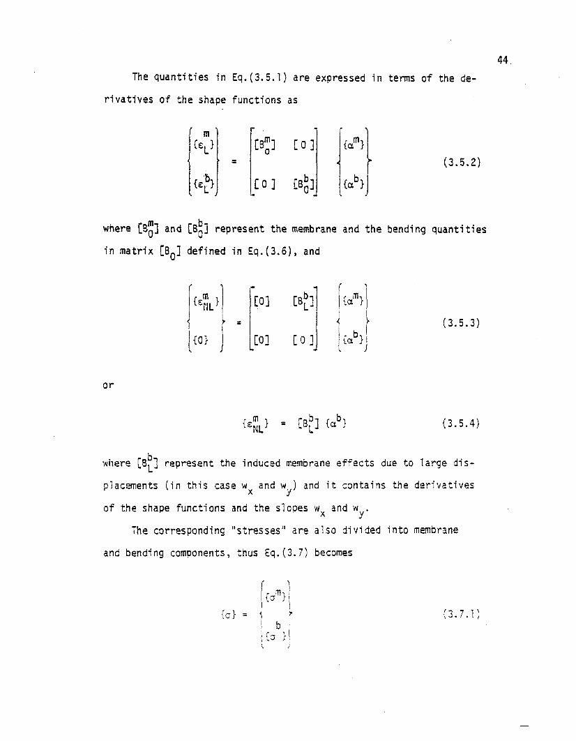
The quantities in Eq.(3.5. 1) are expressed in terms of the de-
rivatives of the shape functions as
m(6m] {am}1{E
L} [0 ]
0=
{ab}J
(3.5.2)b [0 ] [B~J{EL
}
where [B~] and (B~j represent the membrane and the bending quantities
in matrix [80] defined in Eq.(3.6), and
44.
or
={a} [oJ [0 J
(3.5.3)
(3.5.4)
where [8~J represent the induced membrane effects due to large dis
placements (in this case wand w ) and it contains the derivativesx y
of the shape functions and the slopes Wx and wy '
The corresponding II stresses ll are also divided into membrane
and bending components, thus Eq.(3.7) becomes
(3.7.1)

45
The matrix [O*J defined by Eq.(3.11) is written as
[Om][0 ]1
[0*] = (3.11.1)
[0] [Ob] .
where
,- 1 v 0
[Om] = E 1 a (3.11.2)1-v2 v
0 0 l-v2 1
and
v 0
COb] = Et 3v 0 (3.11.3)12(1-v2. )
a 0 l-vT
These definitions enable us to proceed with evaluating the
matrices [BOJ, [B l ], and [KcrJ as illustrated in the following sec
tions.
3.4-A Evaluation of [BOJ
If the nodal numbering scheme for the fiat rectangular bending
membrane element shown in Fig. 3.1 is followed. the displacement
component u(x, y) given by Eq.(3.3) can be written as

u(x,y ) = [H (1)(x) H(1)(y), H(1)(x) H(1)(y), H(1)(x) H(1)(y) ,01 01 11 01 01 11
H(l ) (x) H(1) (y), H(1) (x) H(1) (y), H(1)(x) H(1) (y ) ,11 11 01 02 11 02
H(l)(X)H(l)(y), H(l)(X)H(l)(y), H(l)(X)H(l)(y),01 12 11 12 02 02
H(l) (X)H(l) (y), H(') (x)H(l) (y), H(l) (x)H(1) (y),12 02 02 12 12 12
Ha~)(X)Ha~)(y), Hi~)(X)Hai)(y), H~~)(X)H{i)(y),(1) (1) 1 .
H12 (x)H11 (y)'J { u11 ' ux11 ' uy11 ' uxy11 ' u12 ,
ux12 ' uy12 ' uxy12 ' u22 , ux22 ' uy22 ' uxy22 ' u21 '
ux21 , Uy21,Uxy21 } (3.28)
46
Similar expressions can be written for the displacement components
v and w. This makes it possible to write the linear strain compo
nents in terms of the derivatives of the shape functions and the
nodal displacement parameters as
(3.29)
where [BOJ is a [6 x 48] matrix which has the general partitioned form
............................ 41 ••••••••[BOJ =
[B~ ( 3x32)] [0]1
(3.30)
L
[0 ]. .: [B~ ( 3x16) J:, J
Forms of the matrix [SOJ evaluated for the computer program are
shown in Appendix A.

3.4-B Evaluation of [Bl ]
From Eqs.(3.5) and (3.5.4), we can write
47
{ch .1l
.L 3w) 2
2'3x
1 dW 2
'2(3Y)
(OW) (aw, ia~ ayl !
)
(3.31 )
the right side of Eq.(3.31) can be conveniently written as
1(aw)' I (~) 0'2 ax ax
r(;~)1¥dW)2 =1 ( ~;) =t [C]{8}a
l(~)1(3.32). ay 2
I,aw)( aw, i (ow) (aw)\ax a'll 1 3y 'ax
l Y J
where
(aw) a 1'ax
[e] = 0 (ow) (3.33)ay
l(~;) (aw)ax
and
((aW l1{8} =
ax f(3.34)
I (ow \ I"yll
\ 0 i, )

The quantity {e} is defined by expressing the slopes wand w inx y
terms of the derivatives of the shape functions as
48
(3.35)
or
(3.36)
where [G] is a[2 x 16] matrix which is a pure function of the element
coordinates.
From Eqs.(3.31) and (3.32), we can write
(3.37)
Taking the variations on both sides of Eq.(3.37)
But, it can be shown that
[acHe} = [c]{oe}
(3.38)
(3.39)
Because of a special property* of the matrices [C] and {e} using Eqs.
(3.36) and (3.39), Eq.(3.38) can be written as
where
[8~J :: [C][G]
(3.40)
(3.41 )
*See Ref. (73) page 510 for the special property of the matrices[C] and {G}.
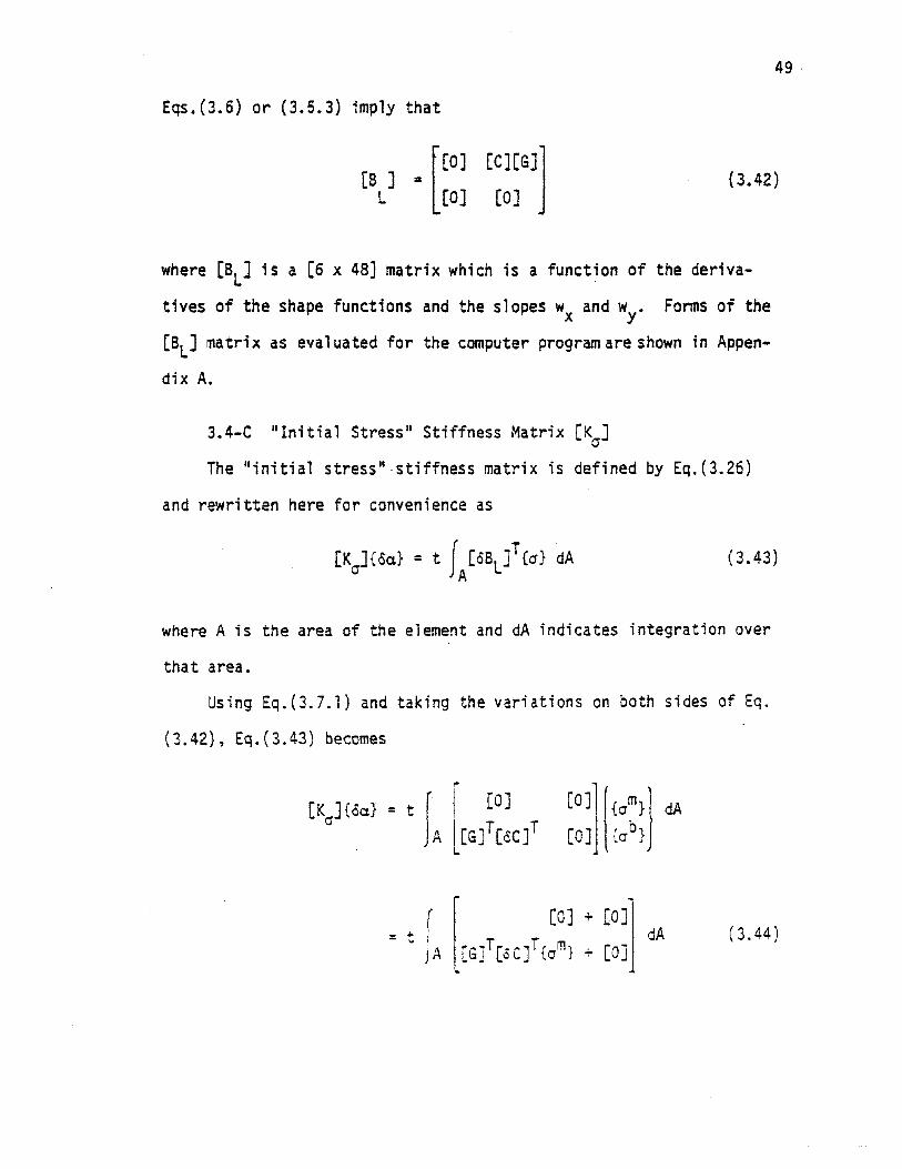
49 .
Eqs.{3.6) or (3.5.3) imply that
[[OJ [CJ(GJ]
[6] =L [0] [OJ
(3.42)
where [BL] is a [6 x 48] matrix which is a function of the deriva
tives of the shape functions and the slopes wand w. Forms of thex y
[6l ] matrix as evaluated for the computer program are shown in Appen-
dix A.
3.4-C "Initial Stress" Stiffness Matrix [K JcrThe "initial stress"·stiffness matrix is defined by Eq.(3.26)
and rewritten here for convenience as
(3.43)
where A is the area of the element and dA indicates integration over
that area.
Using Eq.(3.7.l) and taking the variations on both sides of Eq.
(3.42), Eq.(3.43) becomes
(3.44)
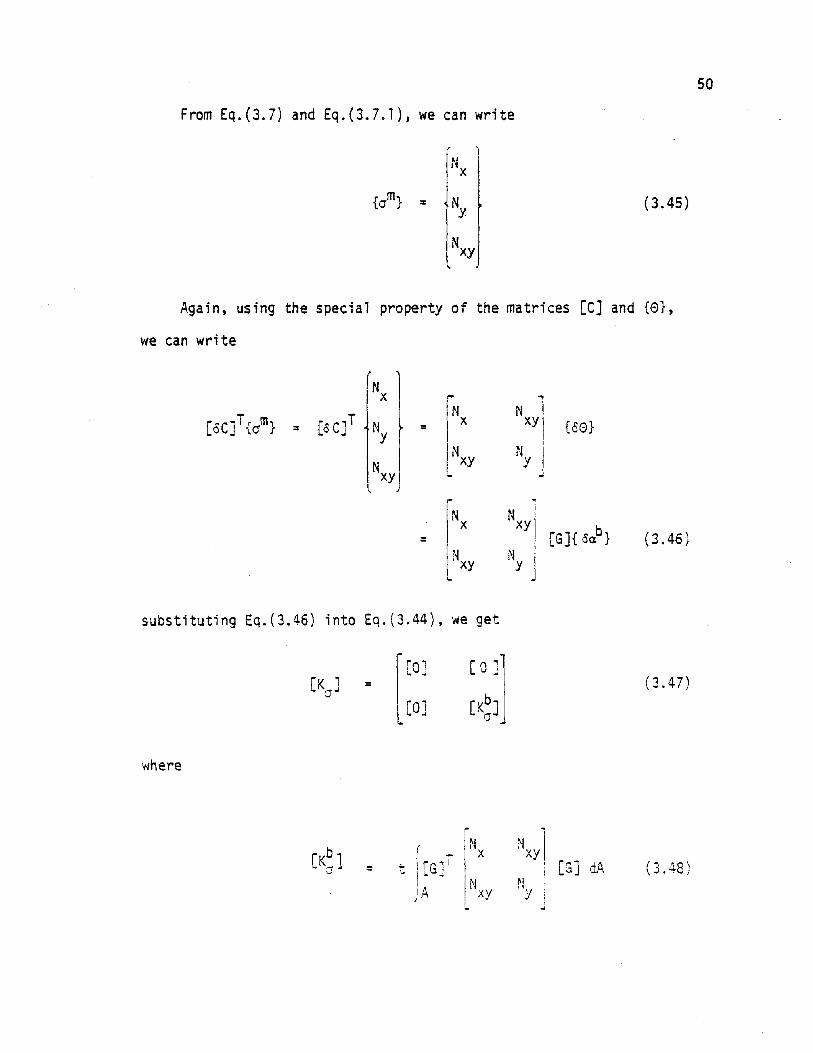
From Eq.(3.7) and Eq.(3.7. 1), we can write
Nx
{om} = Ny
Nxy
(3.45)
50
Again, using the special property of the matrices [C] and {0},
we can write
Nx 1N II l[oC]T{crm} [0 C]T
:yI= x xy {c0}=Nxy Ny J
xy\.
fN NXY]= l~X [GJ{ oab} (3.46)
Ny jI xy
substituting Eq.(3.46) into Eq.(3.44), we get
where
[K Jo =[
rOI.. ..l
[OJ
[ 0 1][K~J
(3.47)
[Kb1 rNx ~l
rG1 T xy= .. [GJ dA (3.48);; I.. I
L. oJ
IN ~I
A "I xy y1..
51
Adding the linear stiffness matrix [KO]' the "displacement" stiff
ness matrix [KL], and the lIinitial stress" stiffness matrix [Ka], the
total element stiffness matrix is obtained as
(3.49)
where [Kr] is the total or IItangential ll stiffness matrix. Expressions
for portions of the matrices [KO]' (KLJ, and, [Ka] , as calculated ;n
the computer program, are shown in Appendices B, C, and D, respectively.
It should be noted that the approach used to derive the stiffness
matrices just shown is attributed to Zienkiewicz (73).
3.5 Equivalent Load Vectors
The concept used in determining the load vector for a structural
system subjected to some loading is that the total work done by the
equivalent loads must be equal to the work done by the actual loads.
In the computer program prepared for this investigation, membrane load
vectors qm for concentrated nodal loads, distributed edge shear loads,
and uniformly distributed in-plane loadings on each of the four edges
of the element are formulated. Similar expressions are also formu-
lated for the bending load vectors due to concentrated nodal loads,
distributed edge moments, distributed edge shears, and uniformly dis
tributed lateral loads.
As an illustration, the calculation of the bending load vector
qb due to a uniformly distributed lateral load q will be demonstrated
here. A displacement, say w in this case, may be expressed in terms
of products of one-dimensional Hermitian interpolation polynomials
as

_ 4 2 [(1) (1) (1) (1)w(x,y) -; ; HOi (x)HOJ' (y)w;i + H'i (X)HOJ· (y)w ..,=1 J=l ~ X1J
(1) (l) (1) (1) J+ HOi (X)H,j (y)Wyij + H'i (X)H,j (y)WXyij (3.50)
52:
For a rectangular flat plate element with dimensions a and b.
along the x and y axes, respectively, the components of the bending
load vector are calculated from
V : of: f: q w(x,y) dx dy (3.51 )
For example, the component of the bending load vector corresponding
to the nodal parameter wx1l at node (1,1) is obtained as '
(3.52)
Substituting the expressions for H~~)(x)l*and Ha~)(y) and carrying
out the indicated integration, we obtain
= ga 2b
24 (3.53)
All components of the membrane and the bending load vectors are
obtained in exactly the same manner (9). Table 3.1 shows the bending
load vector components for a rectangular element due to a uniformly
distributed lateral load.
With all components necessary for computing the large deflection
*The prime on H~~)(X) indicates derivatives.
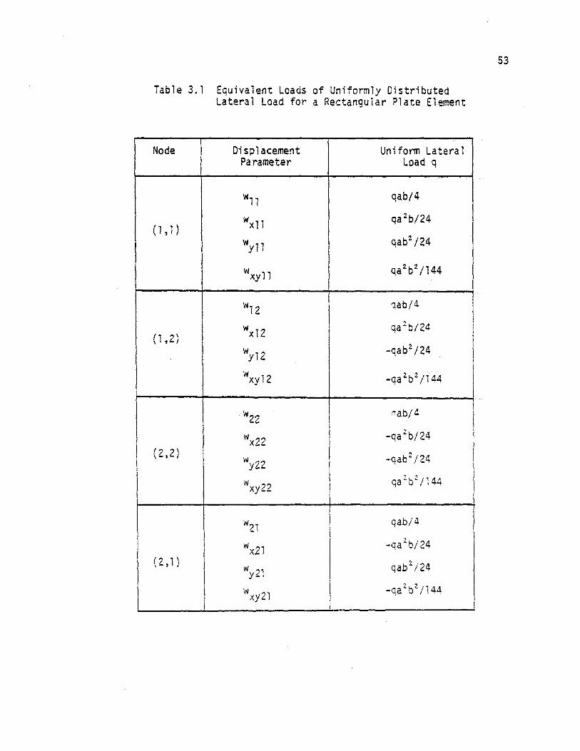
Table 3.1 Equivalent Loads of Uniformly DistributedLateral Load for a Rectangular Plate Element
Node Displacement Uniform LateralParameter Load q
wll qab/4
wxll qa 2 b/24(1,1)
wyn qab2 /24
wxy11 qa 2 b2 /144
wi2 1ab/4
'Nx12 qa 2 b/24(1 ,2)
wy12 -qab2 /24
wxy12 -qa 2 b2 /144
w22"lab/4
wx22 -qa 2 b/24
(2,2) wy22 -qab 2/24
Wxy22qa 2. b2 /144
wZ1qab/4
wx21-qa2. b/ 24
(2,1)w "'1 qab 2 /24y,-
Wxy21\
-qa 2 b2./1 44
53

problem available, the solution of the assembly of all the elements
is accomplished in the usual manner as if the stiffness of each ele
ment were simply the sum of [KO] , [KLJ, [Kcr
] stiffness matrices.
Thus the solution of the nonlinear problem becomes a sequence of
solutions of linear problems in which calculated displacements and
stresses are added to the previous values to give an up-to-date
account of the geometric state of the structure as the applied load
is increased. An outline of the solution technique used in this
work is presented in the next chapter.
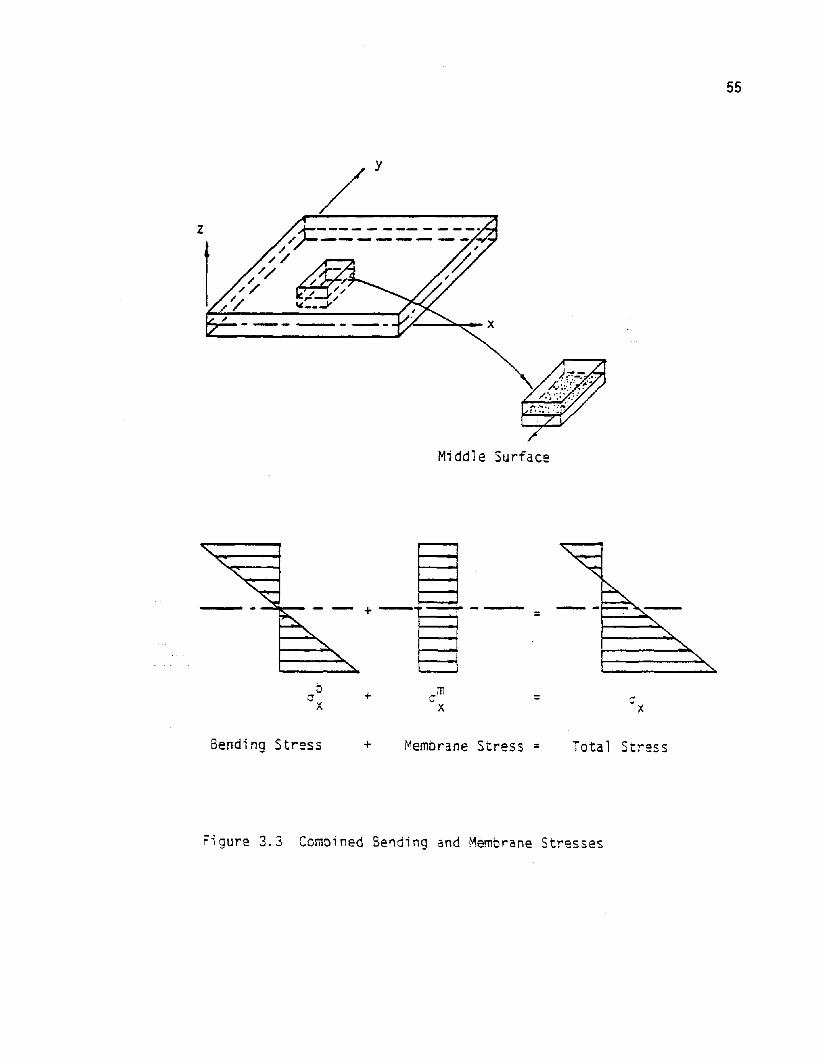
3.6 Combined Bending and Membrane Stresses
The stresses at the middle and outer planes of a plate element
due to the applied external loads are the ones of interest in this
investigation. Figure 3.3 shows that in the x-direction a bending
stress attains its extreme levels at the outer surfaces of the ele-
ment and it is zero at the middle surface, while the membrane stress
is uniform throughout the plate thickness. If this is assumed to
hold true for all stress components, the bending and membrane stresses
can be superimposed to obtain the total stresses acting on the
plate.
For each of the four nodes of the rectangular element the mem
brane and the bending "stresses ll are obtained from the stress-strain
relations indicated by Eq.(3. 10) which may be written in matrix form
as
54
55
z
----------
Middle Surface
=,",-......;::~--- +-
bax + = =x
Bending Stress + Membrane Stress = Total Stress
Figure 3.3 Combined Sending and Membrane Stresses

\1N vy
N axy
= EM (l-v2. ) ax
M ay
M 0xy
'Ii
a
a
a
a
56
0 a 0 0 r€~ 10 0 a a I:m
~x
l-v a 0 0 m-2- Exy
0 t 3 vt 3 0 bEi2 12 x
0 vt 3 t 3 0 b12 i2
Ey
a 0 0 t 3 (l-v) bExy24
h m m d m .were € , E ,an ~ denotex y xyb b db. d' t thEX' 2y ' an Sxy 1n lea e e
calculated from Eq.(3.6).
(3.54)
the membrane strain components while
bending components, all of which can be
The true membrane and bending stresses can then be calculated
using Eq.(3.8) and (3.9). The combined stress components due to
membrane and bending action are obtained at the extreme surfaces of
the plate by simply adding the respective components as
°xy
( - 5""\j. ':I I
The stress components ox' 0y' and crxy calculated at each of the
four nodes of the rectangular element are then used to calculate the
principal stresses at the olate surfaces. The princioal stress equa-
tions being the standard ones for two-dimensional stress will not be
shown here.

These stresses are averaged at nodes that are common to more
than one element. This averaging tends to reduce the error inher-
ent in the displacement approach in which equilibrium condition of
the forces is not completely satisfied.
3.7 A Brief Review of the Development of the Finite Element Methodin Nonlinear Problems
In 1960, Turner, Dill, Martin, and Melosh (68) introduced the
57
finite element method to geometrically nonlinear problems in a paper
in which they analyzed the effects of initial in-plane stress on the
stiffness of stringers (i.e., beam-columns with zero bending stiff
ness) and of plane stress triangle elements. The approach was to
develop the initial stiffness matrices for use in the in~remental
force-displacement relation. Gallagher, et al. (22), substituted
a complete cubic function into the strain energy expression to de
rive the stiffness matrices. Martin (39) reviewed several papers
on the derivation of nonlinear stiffness matrices and concluded
that the same functions need not be used to represent both linear
and nonlinear effects. Kapur and Hartz (30) derived ~stability-
coefficient" matrices for nine independent states of in-plane
stress which represented an extension beyond previous derivations
that were based on only three stress states. Clough and Fe1ippa
(16) made comparison studies of several finite element formula-
tions in plate buckling in which both consistent and inconsistent
approaches were used and found that the inconsistent approach gave
good results. Murray and Wilson (43) used constant stiffness ma-
trices and accounted for all geometric nonlinearities by coordinate

rotations. They noted that their approach was equivalent to using
the Kirchhoff's assumptions for each individual element, rather than
the nonlinear von Karman theory. Mallett and Marcal (36) presented
a unifying basis for formulating the large deflection problems. They
derived the total strain energy as a function of nodal displacements,
using functions and including strain energy terms which previously
had been neglected. Stricklin, et al. (59) applied the matrix dis
placement method in which they employed linear and nonlinear equili
brium equations by separating the linear and nonlinear portions of
the strain energy and then applying the nonlinear terms as additional
generalized forces.
Recent papers on finite element methods in nonlinear plate
analysis have focused on the method of solution. Kawi and Yoshi
mura (31) gave an iterative procedure for solving large deflection
plate problems. Their approach was similar to the unbalanced-force
iteration, but their formulation included all stiffness terms.
Schmit, Bogner, and Fox (56) used a direct minimization technique
for solving large deflection problems of plates and cylindrical
shells. To compute strain energy, rectangular coefficient matrices
were summed with linear and quadratic displacement vectors. Hais
ler and Stricklin (23) developed and evaluated several solution
procedures for geometrically nonlinear problems and concluded that
the selection of solution procedure depends highly on the degree
of nonlinearity the oroblem possesses.
The interested reader is advised to consult the following
references for more understanding of the various finite eiement
58.,

fonnulations of geometrically nonlinear problems (1, -3, i, 11 ,14,
17, 40, 42, 43, 44, 45, 49, 51, and 62).
At this point, it should be noted that the present finite ele
ment formulation is not the only attempt to solve the geometrically
nonlinear rectangular glass plate problem. Tsai and Stewart (67)
used a finite element program developed by Melliere (43) to study
the stress distributions in glass plates. Moore (46) used the
ARGUS nonlinear finite element structural analysis program to
analyze rectangular glass solar panels subjected to uniform normal
pressure loads. The formulation of both above mentioned computer
programs include only constant strains to represent the membrane
behavior of the plate whereas, the present finite element program
includes not only constant strains but also linear strains to
represent the membrane behavior of the plate. Representation of
the membrane behavior as such is important in better assessing the
overall stress distribution within the glass plate, particularly
at the perimeters of the plate.
59
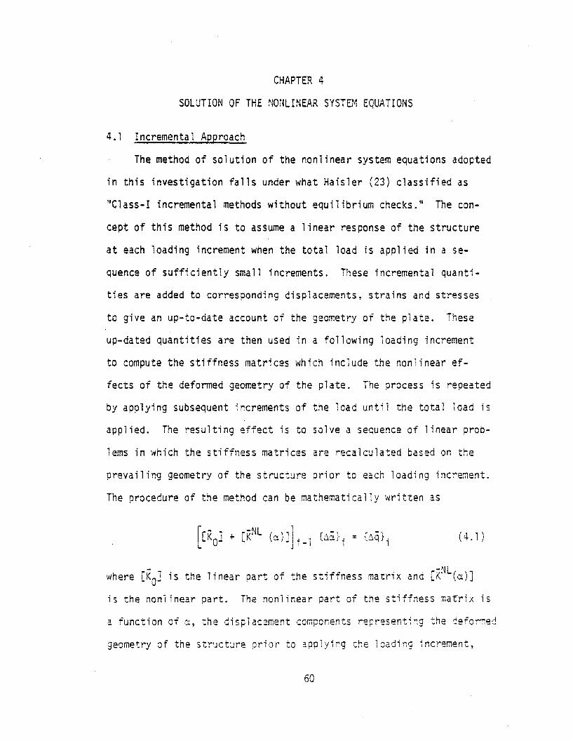
CHAPTER 4
SOLUTION OF THE NONLINEAR SYSTEr1 EQUATIONS
4. 1 Incrementa 1 Approach
The method of solution of the nonlinear system equations adopted
in this investigation falls under what Haisler (23) classified as
"Class-I incremental methods without equilibrium checks. 11 The con-
cept of this method is to assume a linear response of the structure
at each loading increment when the total load is applied in a se-
quence of sufficiently small increments. These incremental quanti-
ties are added to corresponding displacements, strains and stresses
to give an up-to-date account of the geometry of the plate. These
up-dated quantities are then used in a following loading increment
to compute the stiffness matrices which include the nonlinear ef-
fects of the deformed geometry of the plate. The process is repeated
by applying subsequent increments of the load until the total load is
applied. The resulting effect is to solve a sequence of linear prob-
lems in which the stiffness matrices are recalculated based on the
prevailing geometry of the structure prior to each loading increment.
The procedure of the method can be mathematically written as
( d. 1)
h [K- ~. h l' fl.' ~f . and L" -KNL(('.J ) ]w ere oj 1S t e 1near part a tile stlT ness matr1x -
is the nonlinear part. The nonlinear part of the stiffness matrix is
a function of a, the displacement components representing the deformed
geometry of the structure prior to applying the loading ~ncrement,
60

and {~&} is the increment of displacements resulting from applying
the ith loading increment {~q}. After applying the ith loading in
crement the total displacements are obtained by
61
(4.2)
Incremental solution procedures for geometrically nonlinear
problems are presented in the literature in several different forms.
Incorporation of a particular form of an incremental procedure in the
formulation of a geometrically nonlinear problem depends on several
factors such as the degree of accuracy desired, the degree of non-
linearity in the problem, the complexity of the probla~ formulation,
the availability of computer dollars, etc. Haisler (23) and Strick
lin, Haisler, and von Rieseman (58, 59) have made intensive studies
of several solution procedures for geometrically nonlinear problems
and the interested reader is referred to their work.
4.2 Algorithm of the Incremental Apcroach
To solve the geometric nonlinear problem under investigation
using the proposed finite element formulation, the following algor-
ithm is used for the incremental approach.
During the ith step, an incremental load vector {6q}i is applied
to the assembled elements of the plate to yield an incremental dis-
placement vector {~a}i' For each element of the structure at the
end of the ith step:
l. Determine current deformed geometry of the element by
adding the resulting incremental displacement vector to
the total displacement vector

{a}. = {a}. , + {6a}.1 , - I 1
(4.3)
62
2. Calculate corresponding strain components by formulating
the [8J matrix which is a function of the derivatives of
the shape functions and only Wx and wy of the displace
ment vector {a}i
{S}. = [S]. {a} .1 1 1
(4.4)
3. Calculate corresponding stress components using the re
lation
to}. = [O*]{s}.1 1
4. Ca 1culate [KO] and [KLJ using
[KO] + [KLJ =J [B]T[O*][B] dV\'I
5. Calculate [KbJ usingcr
r N1
fv[GJT ~l 1
[KbJ = lNxI xy I[G] dVcrNy jxy
(4.5)
(4.6)
(4.7)
6. Repeat algorithm 1 through 5 for all elements and assemble
the global stiffness matrix for the e~tire structure.
7. Apply the next loading increment {6q}i+l to the assembled
structure and calculate {6a}i+l by solving the simultaneous
equations of equilibrium.

(4.8)
&3
8. Repeat algorithm 1 through 7 until the entire load is ap
pl i ed.
The incremental approach outlined above is schematically outlined
in Fig. 4.1.

64 -
a
{D. a} ii -1 ,....+----...,..~
;
;+1
q{~q} i
i-I
r A \t",q, ;+1
;+1
Figure 4.1 Incremental Approach

CHAPTER 5
NUMERICAL EXAMPLES
Four examples of simply supported unifvrmly loaded large de
flection rectangular thin plates are analyzed in this chapter to
demonstrate the validity and versatility of the finite element form
ulation presented in this t.nvestigation. Results are then compared
with theoretical solutions and experimental data available in the
literature. Although the program formulation is capable of analy
zing various types of boundary conditions such as clamped or free
edges, and different combinations of loading such as concentrated
and uniformly distributed' static loads, only problems pertinent
to this investigation are presented here.
In the example problems treated, results of two classes of
simply supported rectangular thin plates with uniform static loads
are shown. These results show the difference which is mainly due
to the prescribed boundary conditions in the plane of the plate.
This difference is described in more detail in appropriate sections
of this chapter. The uniform static loads are replaced by equiva
lent concentrated loads at the nodes as described in Chapter 3.
Uniform and non-uniform discretization schemes of the plate struc
ture are employed in this dissertation to assess the effects of the
boundary conditions.
Due to limited research funds and the lengthy CPU time consumed
by each run of tne computer program, the discretization of one quarter
of the plate is iimited to a grid size of 16 elements. AlSO, the
65

number of loading increments is limited to 100 when the grid size
of one quarter of the plate is 9 elements.
5.1 Simply SupDorted RectangularPlates: Edge Displacement =0
Levy (34) called the boundary conditions of this class of prob
lems flEdge Displacement = 0,11 while Timoshenko (65) named them lIim_
movable ll edges. In this class of problems, the boundary edges of
the plate are assumed to be laterally supported and free to rotate
along the edges in the lateral direction. In the transverse direc-
tion, they remain completely restrained from having any displacement
along these edges in the plane of the plate. These boundary condi
tions were mathematically formulated and shown in Chapter 2. Two
examples of this class of problems are shown in the following sec
tions. The first example problem exhibits results of a simply sup-
ported square thin plate with a uniform static lead and the second
illustrates results of a simply supported rectangular olate with
an aspect ratio of 1.6 and a uniform static load.
5.l-A Example I. Simply Supported Uniformly Loaded SquarePlate: Edge Displacement = 0
In this example, a 10-inch simply supported square plate which
has a constant thickness of 0.04 inch is subjected to a monotoni-
cally increasing static lateral load of 1.837 psi. The elastic
constants of the material of the plate are assumed to be 27.6 x
106 psi for the Young's modulus of elasticity and 0.316* for the
~The value of 0.316 is used to agree with that in Levyls (34) solution.
66

Poisson's ratio. Because of the double symmetry, the problem is
modeled by discretizing only one quarter of the plate. In this
example, a grid size of 2 x 2 elements of equal areas ~s used.
The total load is applied in 40 equal increments and the results
agree reasonably well with Levy's solution (34).
Fig. 5.1 shows a non-dimensional plct* of the deflection of
the center of the plate vs. the applied load. A maximum deflection
of nearly twice the thickness of the plate is attained dS shown in
the curve of Fig. 5.1. The curve clearly indicates the nonlinear
load-displacement relationship involved in this problem, where the
displacement does not increase proportionally as the ioad is in-
creased. This effect is due to the increased stiffness of the
plate whicn in turn is a result of the membrane effect induced by
large lateral displacements.
Membrane and bending stresses are also plotted against the
load and are shown separately. Stresses at different points on
the plate are drawn so that direct comparison with Levy's sOlution
is possible. In Fig. 5.2, Curve A shows the bending stresses v~ or
cr~ of the extreme fibers at the center of the plate while Curve 8
ind~cates the shearing stress due to bending cr~y of the extreme
fibers of the upper right corner of the p1ate. It should be noted
that the difference in the two solutions as revealed in Curve 8,
is believed to be due in part to the coarse discretization since
"'t.;l"less otherwise stated, non-dimensional plots a"'e used throughouttnis investigation so ':hat arbitrary dimensions of square and rectangular plates with arbitrary material constants may be used forcomparison.
67

..-
~ :::!!ne~-:s
:.oJ !:!c~e~e~ts
I___--'-_.....:1 _ :~
68
jO . .: :;C . : 1 • ~ ~
-;\,,; .'~ Z-:G. : 2;0. ]CC.c
Figure 5.1 Load-Deflection of Simply Supported SquarePlate; cdge Displacement = a
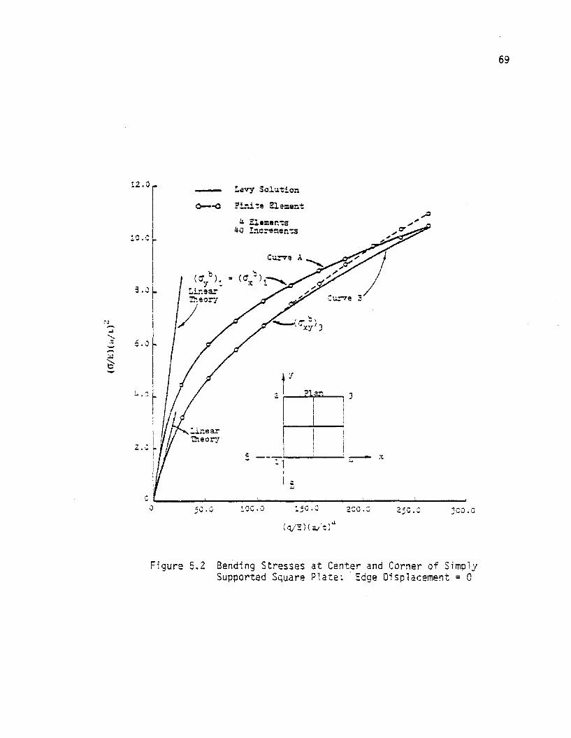
69
12.0tevy Solu,1:ion
?i.-u ':e Elelllen"t
Jco.a2CC.:J
~ :r
21i--<;.a'='1IF1
?+'----'1 J
, I 1
I I! II Ii ,
;"1..-------- =--- ;<:
1.0e .. 0
4 Elemen-ts40 !:tc:rel:len,:s
50.a"L.- ...... ...... ....;, ___
III
3.0 ~
!I
Il
6.0 ~
I:':'.J I
,I
II
~ . I'.v f-.
!II!
lOtC
Figure 5.2 Bending Stresses at Center and Corner of SimplySupported Square Plate~ Edge Oisplacement = 0
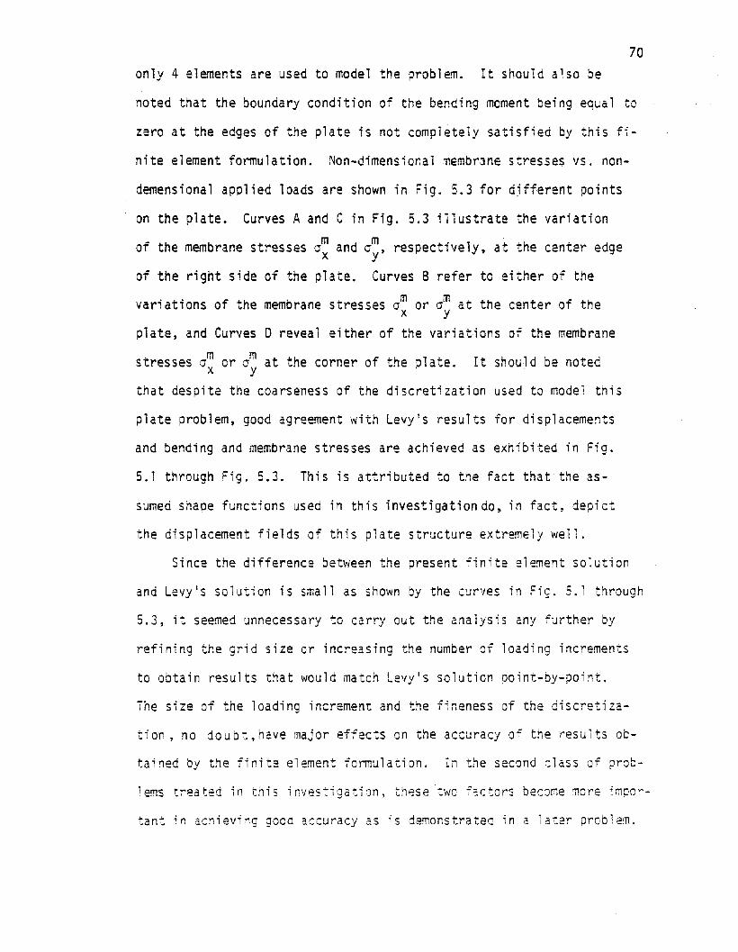
70
only 4 elements are used to model the problem. It should a~so be
noted that the boundary condition of the bending moment being equal to
zero at the edges of the plate is not completely satisfied by this fi-
nite element formulation. Non-dimensional membrane stresses vs. non-
demensional applied loads are shown in Fig. 5.3 for different points
on the plate. Curves A and C in Fig. 5.3 illustrate the variation
of the membrane stresses a~ and a~, respectively, at the center edge
of the right side of the plate. Curves B refer to either of the
variations of the membrane stresses am or am at the center of thex y
p1 ate, and Curves 0 reveal ei ther of the vari ati ons of the membrane
stresses am or om at the corner of the plate. It should be notedx y
that despite the coarseness of the discretization used to model this
plate problem, good agreement with Levy·s results for displacements
and bending and membrane stresses are achieved as exhibited in Fig.
5.1 through Fig. 5.3. This is attributed to the fact that the as-
sumed shape functions used in this investigation do, in fact, depict
the displacement fields of this plate structure extremely well.
Since the difference between the present finite element solution
and Levy's solution is small as shown by the curves in Fig. 5.1 through
5.3, it seemed unnecessary to carry out the analysis any further by
refining the grid size or increasing the number of loading increments
to obtain results that would match Levy1s solution point-by-point.
The size of the loading increment and the fineness of the discretiza-
tion, no doubt,have major effects on the accuracy of tne results ob-
tained by the finite element formulation. In the second class of prob-
lems treated in t,r,is investigation, these t'I'JC factors bec:)I'Tie ~ore impor-
tant in achieving good accuracy as is demonstrated in a later problem.

71
_ !..aV"'J Solu;ticn
0---0 ?ini te Elemen't
(_:II, = f~ :n)\.Ix I!, ''J':
~ nemen'ts(;.0 Increments
J
~ Curie J_~--Q---<J-T .-<J
A- _-:>-_ ... ,Q-t--
?lan
Q~_~+-_--l~_'" _ :t11 ..
I
I Q....
0.0
1I
..;..0 l..
I2. CL
iII
Ii
3.0
10.0
12.0 i
Figure 5.3 Membrane Stresses at Center, Center Edge,and Corner of Simply Supported Square Plate;
Edge Displacement = a

72
5.1-8 Example II. Simply Supported Uniformly Loaded RectangularPlate: Edge Displacement =0
A 96.0-inch long, 60.0-inch wide and 0.25-inch thick aluminum
plate subjected to static lateral uniform load of 0.70 psi is used in
this example. The Young's modulus of elasticity and Poisson's ratio
for aluminum are 10.6 x 10⁶ psi and 0.33, respectively. One quarter of
the plate is discretized into nine rectangular elements of different
areas. The elements with smaller areas are placed along the edges of
the plate as shown in Fig. 5.4. The total load is applied in 50 equal
increments in order to obtain the load-deflection relationship exhibited
by the dashed curve in Fig. 5.4. The sol id 1ine shown in the figure
represents an approximate solution attributed to Timoshenko (65); calcu
lations for this curve are reported by Anians (2).
As was demonstrated in the example of the previous section, bending
and membrane stresses are plotted separately for different points on the
plate. Variations in bending stresses are shown in Fig. 5.5 at theb bcenter and at the corner of the plate. Bending stresses ax and cry are
indicated by Curve B and Curve C, respectively. As expected, the bending
stress parallel to the shorter side of the plate, in this case a~, is
larger than the bending stress parallel to the other side. However, the
general behavior of the center bending stresses, particularly parallel to
the shorter side of the plate, is similar to that of a square plate. It
can be noted by examining Fig. 5.5 that cr~ varies almost linearly after
the load (q/E) (b/t)4 reaches a magnitude of about 48.0. The shear stress
due to bending a~y at the corner of the plate is indicated by Curve A. It
should be noted that this shear stress has a comparable or larger magnitude
than the center stress in this plate. The opposite was the case for the

73
______ Timcshenko's ~pproxi~ate Solu~ion
0---0 ?inita Element
250 . .:200.0
?:an
l50.C
!I
~_._~:__....... ~...' _ :t
I
IE
100.0
9 Elements50 !nC:'9ments
;0.0
"'"Linear'~eory
2.0
.....t.5~
... I" I;: I
I-- il.°rI
0.; ~iIi
0Q
Figure 5.4 Load-Deflection of Simply SupportedRectangular Plate~ Edge Displacement = 0'

74
?bite necent
9 Elements50 !nerements
I
iIII
6.0 lti
Iii
:., 0 ~
01:-' -....~---:'_!L-..--........J'-----l------Jo 50.0 ~oo,c ~5C.: 2CC.C 250,0
Figure 5.5 Bending Stresses at Center and Cornerof Simply Supported Rectangular Plate:
Edge Displacement = 0

75
corresponding stresses in the square plate (see Fig. 5.2). In Fig. 5.6,
membrane stress variations in the x and y directions are shown for the
center, the center of the short edge, and the corner of the plate, and
are indicated by Curves A, B, C, D, and E. It should be noted that the
magnitudes of o~ and o~ at the corner of the plate differ slightly but
the difference is so small that it cannot be shown in the figure.
5.2 Simply Supported Rectangular Plates: Edge Displacement 1 0
In this class of problems, the boundaries are also assumed to be
laterally supported and free to rotate in the lateral direction. But, it
is also assumed that the plate edges can move in the plane of the plate.
Levy (34) presented a plate solution of this type in which he assumed that
the plate edges could move in-plane, but were constrained to remain straight.
Levy termed this set of boundary conditions "Edge Compression = 0." These
boundary conditions assumed by Levy do not define the actual edge conditions
of the thin glass plates under investigation. The edges of typically
installed glass plates can translate in the plane of the plate, and do not
necessarily remain straight. This fact was confirmed experimentally by
Anians (2) who measured the in-plane edge displacements of a laterally
loaded window glass plate installed in an actual framing system. Kaiser (29)
presented a solution for a uniformly loaded, simply supported square plate
with edges that are both free to move and distort in-plane. He used a
finite difference formulation to solve the nonlinear plate equations and
compared his results with data obtained from an experiment which he conducted
on a square plate. Results obtained from the present finite element
formulation are compared with Kaiser's solution.
Differences in the in-plane boundary condi~ions of simply supported
plates, as defined by Levy and Kaiser, result in a substantial difference

76
F:'nite ::lement
9 ::laments50 !nc=-emen'ts
4.0
a.CL
lZ.J[ I I
£ I I1,0.0 :-' ...... _U ~ X
( q,/! ) (0/ :: ) i.;.
Figure 5.6 Membrane Stresses at Center, CenterEdge, and Corner of Simply SupportedRectangular Plate; Edge Displacement = 0

77
in the center deflection results obtained in each case as shown in Fig. 5.7.
For example, when Levy (34) compared his results for IIEdge Compression = 0"
with Kaiser1s sOlution he found that a load of (q/E)(a/t)4 = 118.8, the
center deflection obtained by his method was about 25 percent lower than
the center deflection obtained by Kaiser.
Two examples in this class of simply supported rectangular plate problems
are demonstrated using the same plate dimensions used in Example I and
Example II in Section 5.2. In the first example, center deflections and
bending and membrane stresses are plotted against applied loads. Effects of
the size of the loading increment and the fineness of the discretization on
the stresses are illustrated. Center deflections of a rectangular plate
calculated 'in the second example are compared with experimental results
obtained by Anians (2). Finally, membrane and bending stresses at the center
of the plate are plotted against the applied loads.
5.2-A Example I. Simply Supported Uniformly Loaded Square Plate:Edge Displacement ~ 0
The square plate problem analyzed in Example I of Section 5.l-A is
analyzed again in this section. In this analysis, it is assumed that the
edges of the plate are free to move in the plane of the plate and do not
necessarily remain straight. In order to compare results with Kaiser1s
solution (29), the lateral load is changed to 0.83 psi and is applied to
the plate structure in 100 equal increments. Also, one quarter of the
plate is idealized by nine rectangular elements of different dimensions.
This scheme is adopted for this problem so that discretization errors at
the edges of the plate are minimized.
The center deflection obtained by the finite element solution is
compared with Kaiser's solution in Fig. 5.8. A center deflection larger

78
ljC.C
I2.Cr
I
II
I
I~ "I-'T
I
IIIIi
J~I ~~ """" ---'jC.O :~:.:
Figure 5.7 Effect of Boundary Edge Conditionon Center Deflection of SimplySupported Square Plate
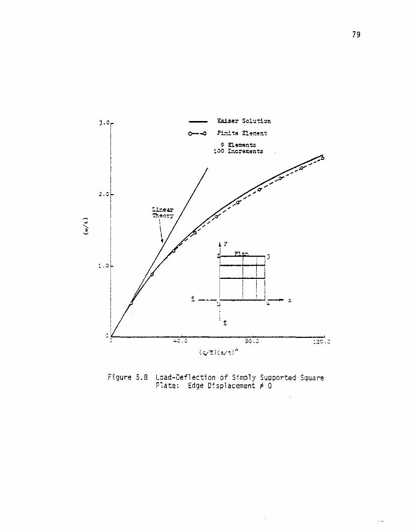
J.O0--0
Kaiser Solution
Fi:ti. te Elo!::ent
9 Elemen"ts1,00 Increments
79
JIII
:.0
c '- ~,,~~.....~, -:-....... -"~v.~ 30.0 12C.J
( ;IE )(a/-: )..:.
Figure 5.8 Load-Deflection of Simply Supported SquarePlate: Edge Displacement f 0

80
than twice the thickness of the plate was attained. Obviously, this is well
within the nonlinear range. The stiffening of the plate with increasing
deflection is again indicated by the decreasing slope of the curve. It
should be noticed that the center deflections obtained by the finite element
method are slightly lower than those obtained by Kaiser, but uniformly so
throughout the application of the load. This difference is partially attri
buted to the coarse finite element discretization, particularly at the
center of the plate (see diagram in Fig. 5.8).
Membrane, bending, and total stresses are plotted against the load in
Fig. 5.9. Agreement of bending stresses with Kaiser's solution ]s not as
good as the agreement between membrane stresses. However, both the finite
element solution and Kaiser's solution are subject to numerical errors.
Differences are also apparent in comparisons of total stresses which are
simply the sum of the bending and membrane stresses. It should be noted
that, for clarity, results of only every 10th loading increment are indicated
on the curves of Fig. 5.8 and Fig. 5.9.
The effects of the size of the loading increment on the accuracy of the
center deflection, bending, and membrane stresses are studied in this example.
The above plate problem is solved using the same dimensions, elastic constants,
and discretization scheme with the loading applied in 20, 50, and 100 equal
increments. The effect of the size of the loading increment on the center
deflection is revealed in Fig. 5.10. The convergence of the deflection
improves as the number of loading increments is increased. The center
deflections obtained when applying the load in 20, 50 and 100 increments are
slightly lower than those obtained by Kaiser1s solution, but uniformly so
throughout the load. These comparisons indicate that the deflections of

81
~iser Solution
0---0 Fir.i te !lemen1;
9 !lements100 Increments
iS
i 11 I i
7~
2 ;.-1__Q..'..."..n......,~ JI I I
~--
IlZ.O r
IIiI
.3.0 i..i
i
II!
:':'.J ~
"-C.O
Figure 5.9 Bending, Membrane, and Total Stresses atCent~r of Simply Supported Square Plate:Edge Displacement f 0
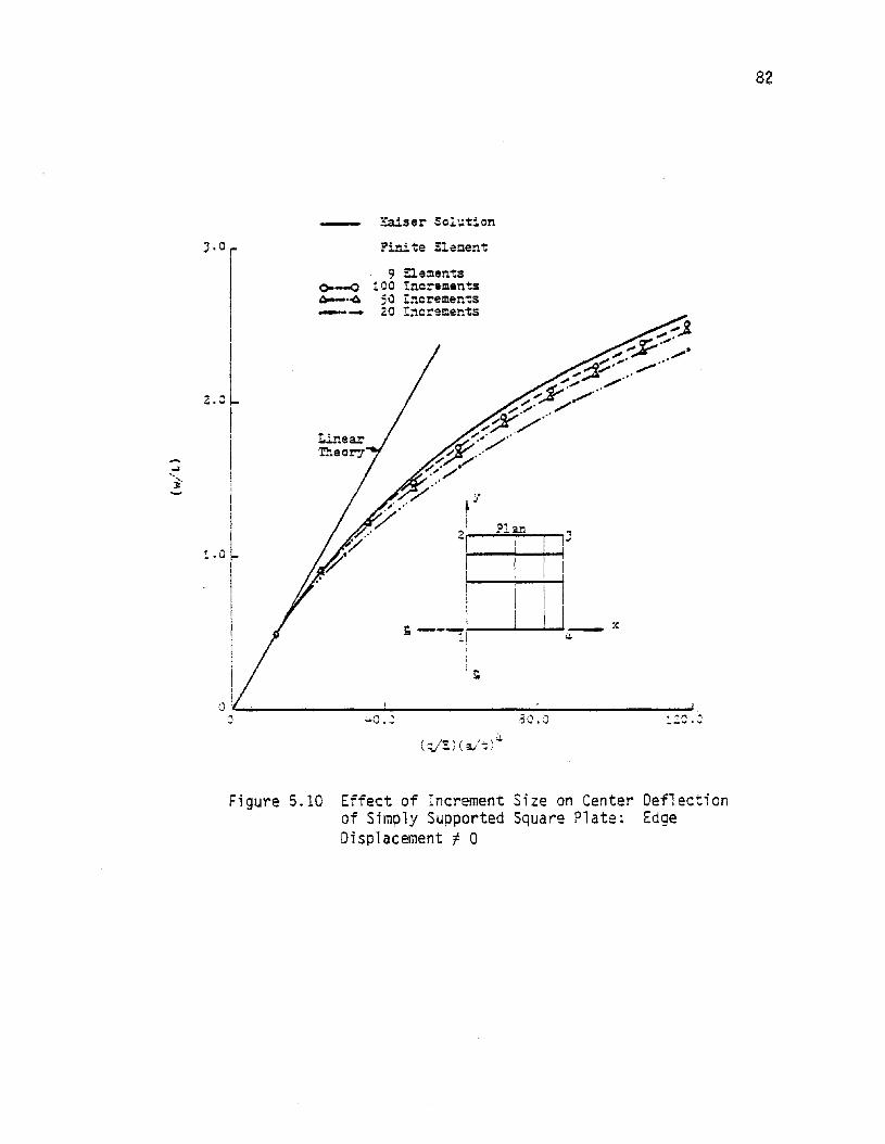
82
Kaiser Sol·.1~ion
Fini1:e ::leClent
::c.:
J
t
3C.J
21 'lAiJ! I I I .s---' I. __ .t11 !.;.I
II~
w.O.J
9 Elements<>--0 100 !nc:-ements6--..0. ;0 !ncremen'ts-- ,0 !;lcrements
J.er
II
z.eltI
..... I..... I'i- 1
I
II
Ii
1..0 ~IIIIIIII
IIII
i0;J
Figure 5.10 Effect of Increment Size on Center Deflectionof Simply Supported Square Plate~ EdgeDisplacement! 0
83
the plate are well represented by the finite element formulation when 100
load increments are used.
Parallel to the comparison of results made in Section S.l-A, the
bending stresses at the center and the corner of the plate are shown in
Fig. 5.11. Central stresses are a1 so compared with those obtained by
Kaiser (29). In Fig. 5.11, it is indicated that as the number of loading
increments is increased, the magnitude of the bending stress at the center
of the plate decreases while the corner shear stress increases.
Figure 5.12 illustrates effects of the number of loading increments
on the membrane stresses at the center and the corner of the plate. The
stresses at both locations appear to converge as the number of loading
increments increases. Confidence is further increased by the reasonably
good agreement of the center membrane stress with that obtained from Kaiser's
solution. It should also be noted that the stress at the edge center of
the plate is a compressive stress, indicating distortion of the edges of
the plate.
When studying the effect of discretization on the accuracy of the
finite element plate model one quarter of the square plate used above is
idealized with 1, ~ and 9 elements and the load is applied in 50 equal
increments. (Fifty increments are used to solve the problem; once for
one element discretization and again for four element discretization.
Results of displacements and stresses are already available for the 9
element discretization.)
The effect of the discretization on the bending stresses at the
center and the corner of the plate is shown in Fig. 5.13. These
stresses converge as the discretization is refined. Convergence also
occurs for membrane stresses at the center and the edge center of the
plate, as indicated in Fig. 5.14.

84.
I !I I$---: ~I_--i---'-.-..-:;:--:c
~ser Solution
I
IE
Fini':e ::lement
9 ElementslOa Increments
.50 Increments20 Inere:ents
-
O~ -:--"'- ~~ ~~
o ~O.J 80.J 120.0
4.0 rI
!Z.O I
IIiI
5.0 ~I
16.0 rII
Figure 5.11 Effect of Increment Size on Bending Stresses atCenter and Corner of Simply Supported SquarePlate~ Edge Displacement 1 a

85
16.~ !.aiser Solution
Finite Element
9 !laments00--<) 100 Increments~ SO Increments
20 Increments
120.0
t:l, "..
I
I I Ie __~ It
J~=:::::;;" ~.l..- ~
C 40.0 80.0
12.0
,.... I-- ,~
d i- o.:;~-- i:.:!
i /~
(q/!) (a!t)J.
Figur~ 5.12 Effect of Increment Si ze on Membrane Stresses atCenter and Center Edge of Simply Supported SquareP1ate; Edge Displacement 1 0

86
./
uiser Sol·..::':i~n
;0 !:lc::'~!:le~-:s
1. ne::en~
~--4 ~ El:~en~3
o--~ 9 !lsmen-:s
l y
2i-'---""'"TJ
~ ---,I-
*
o ,'(,. ~~------~...:....---------"o ~O.J ao.o
I e I:Z.O !
r ...1.1
I I
I I
I:~
IfI
i
-. /::- .
! /-- a ,!~ i--.(:J
~I
Ii
II
I,I
-.= Ir;
Figure 5.13 Effect of Discretization on Bending Stresses atCenter and Corner of Simply Supported SquarePlate: Edge Displacement ~ 0

37
:6.0
• '.I2 ....1 ~J
e.... -,l..lo'------':r- x
I's
Finite Elelr.ent
9 nemer.ts
Kaiser Solu'tion
SO Increments1 ::le~ent!.:. Elaments
_......
o,:--==-- ~~~-----__::~_:_-----~~c ~o.o ao.C :20.8
I
Ii
:...cL
!
iIII
I
!
12.0rII\
II
a.JL
I
Figure 5.14 Effect of Discretization on Membrane Stresses atCenter and Center Edge of Simply Supported SquarePlate~ Edge Displacement 1 0
88
Effects of the number of loading increments and the discretization on
the accuracy of the finite element solution are discussed later in more
detail.
5.2-B Example II. Simply Supported Uniformly Loaded RectangularPlate: Edge Displacement; a
The aluminum rectangular plate problem analyzed in Example II of
Section 5.l-B is solved in this example assuming simply supported edges
that are free to move in the plane of the plate and are not constrained to
remain straight. The load is applied in 100 equal increments to obtain
the variation of the center deflection of the plate shown in Fig. 5.15.
It should be observed that the axes of the load-deflection curve are
expressed in terms of loads and deflections expressed in units of psi and
in. t respectively. The curve is plotted in this manner in order that a
point-by-point comparison of the finite element solution can be made with
experimental data presented by Anians (2).
Anians (2) studied the center displacements of an aluminum plate
mounted in an actual window glass framing system similar to that presented
in Fig. 1.1. To assure that the aluminum plate was free to slip in-plane,
the interface between the aluminum plate and the neoprene gaskets was
lubricated prior to testing. To further assure that the plate edges were
free to slip in-planet the outer neoprene gaskets were installed only near
the plate corners to resist localized corner uplift. Center deflection
results measured by Anians are compared to theoretical results generated
with the finite element analysis in Fig. 5.15.
As is the case in all deflection curves presented preyious1y in this
investigation. the deflection curve obtained by the present finite element
formulation reveals the stiffening of the plate with increasing deflection.
This effect is indicated by the decreasing slope of the curve. It should

89
Fir.i.te Element
1.)0---0
9 Elements100 Increments
?lan
:J1
I
LinearTheot"J
V
21 rJ
. I--+-~l_ ,11 ~
I
le;J ':- ~'_'"" ---'
J 0.2 ,J.'" 0.6 0.3
:'.0
\'l.l;
--= :...
I~
O.Sr
'.. in psi
Figure 5.15 Load-Deflection of Simply Supported RectangularPlate~ Edge Displacement ~ 0

90
be noticed that there is an excellent agreement between the displacement
results obtained by Anians and theoretical results up to a central deflec
tion of three times the plate thickness as illustrated in Fig. 5.15; At
that point, the theortical deflections tend to be less than the measured
deflections. This condition is attributed to the fact that the lateral
displacement along the perimeter of the plate is assumed to be zero in
the present finite element formulation, while in Anian's experimental work
the neoprene gaskets along the plate perimeter allowed the edges to move a
small amount in the lateral direction.
In Fig. 5.16, bending and membrane stresses at the center of the
plate are shown. The effect of the boundary edge conditions is clearly
evident if the value of the membrane stress in the y-direction is compared
with that presented previously in Fig. 5.6.
5.3 General Remarks and Discussion of Results
The preceding sections of this chapter included example problems
involving large displacement-small strain, simply supported, uniformly
loaded, square and rectangular plates with two different in-plane boundary
conditions: Edge Displacement = 0 (Examples I and II in Sections 5.1-A
and 5.1-B), and Edge Displacement r 0 , where the edges do not necessarily
remain straight as the plate is deflected (Examples I and II in Sections
5.2-A and 5.2-8, respectively). The validity of the proposed finite ele
ment formulation has been demonstrated for specific large displacement
square ann rectangular plate problems by comparison with closed form solu
tions. The finite element technique also can be applied to plates of
rectangular shape with boundary edge conditions for which no closed-form
solution exists.

91
9 Elemer.'tslaO !ncr~ments
?~~ ,-;'....' .\,.,zeo.;:00.0
I I
Figure 5.16 Bending and Membrane Stresses at Centerof Simply Supported Rectangular Plate:Edge Displacement f 0

It was noted from the numerical studies conducted on the prob
lem in Example I of section 5.2-A that the convergence of stresses
to exact values differs between bending and membrane stresses, and
depends on the fineness of the finite element discretization, the
location within the plate, and the relative magnitude of the load
ing increment. This difference can be outlined as follows:
1. As the number of loading increments is increased the con
vergence of the bending
a) Stress at the center of the plate approaches
the exact value from an upper bound,
b) Stress at the corner of the plate approaches
the exact value from a lower bound,
and the convergence of the membrane
a) Stress at the center of the plate approaches
the exact value from a lower bound,
b) Stress at the center edge of the olate approaches
the exact solution from a lower bound.
2. As the size of the discretized ele~ent is reduced the con
vergence of the bending
a) Stress at the center of the plate approaches
the exact solution from an upper bound,
b) Stress at the corner of the plate approaches
the exact value from an upper bound,
and the convergence of the membrane
a) Stress at the center of the plate approaches
the exact value from an upper bound,
92

b) Stress at the center edge of the plate approaches
the exact value from an upper bound.
93

CHAPTER 6
CONCLUSIONS AND RECOMMENDATIONS
In this investigation, a finite element displacement approach
formulation has been presented for obtaining numerical solutions to
geometrically nonlinear large displacement-small strain problems of
rectangular thin elastic plates. It has been demonstrated that the
method is capable of solving rectangular plate problems in which
membrane and bending behaviors are coupled and that displacements
and stresses, particularly membrane stresses, are sufficiently ac
curate for engineering purposes.
It should be noted that in most finite element research dealing
with geometrically nonlinear plate problems, the membrane behavior
of the plate is represented by simple shape functions which include
only constant strains. In this research, the membrane behavior is
modeled by products of one-dimensional Hermitian polynomials of order
one. Thus, the resulting shape functions are polynomials capable of
representing not only constant strains but also strains which vary
linearly within the element. Representation of the membrane be
hdvior as such is important in studying the stress distributions in
the glass plate, particularly at the perimeters of that plate. This
approach furnished results that are in very good agreement with avail
able ~heoretical and experimental data. Based on the resul~s obtained
from this research, the following ~onclusions have been made.
94

95
1. The proposed finite element formulation fulfills the ob
jective of the investigation.
2. The glass plate which has edges that are free to move in
plane experiences larger central stresses and displacement
than plates with lIilTl1'lovable ll edges.
3. Appreciable compressive membrane stresses which have
maximum values at the center edges develop along the peri
meters of the plate.
4. Convergence of stresses differs between bendinq and
membraDe stresses and deoends upon the fineness of
the finite element discretization, the location within
the plate, and the relative magnitude of the loading incre
ment.
The present research has given a means by which the stress dis
tribution in rectangular plates can be studied. However, as with any
research, this investigation must be continued. Therefore, it is
recommended that certain improvements be made on the computational
scheme of the proposed approach and that certain topics be pursued
1. Improve the computational scheme by checking the equili
brium at each loading increment and using a geometric
progression type incremental approach.
2. Conduct more studies of edge stresses of the glass plate
problem by using a finer mesh size along the boundaries and
plotting separately the variations of bending and membrane
stresses at critical points in the plate.

3. Compare stresses at critical points of the plate that
develop when the edges are free to move in the plane of
the plate with those developed when the edges are re
strained.
4. Conduct corner stress studies when the corners of the
glass plate are allowed to lift.
S. Model the perimeters of the glass plate as plates on
elastic foundations and impose rotational elastic
springs along those perimeters to include the effects
of the partial res~raint placed by the window framing
system on the plate.
6. Compare total stresses with available experimental data
on glass.
96

LIST OF REFERENCES
1. Allman, D. J., "Some Fundamental Aspects of the Finite ElementAnalysis of Nonlinear Elastic Plates," Finite Element Analysis in Nonlinear Mechanics, 1st Conf. on Finite Element inNonlinear Solid and Structural Mechanics held at Geilo,Norway, in August, 1977, pp. 345-371.
2. Anians, D. C., "Experimental Study of Edge Displacements ofLaterally Loaded Window Glass Plates," Master Thesis, TexasTech University, 1979.
3. Argyris, J. H., Recent Advances in Matrix Methods of StructuralAnalysis, Pergamon Press, London, 1964.
4. Bauer, F., Bauer, L., Becker, W., and Reiss, E. L., "Bendingof Rectangular Plates with Finite Deflections," Journal ofApplied Mechanics, Trans. of the ASCE, December, 1965, pp.821-825.
5. Bazeley, G. P., Cheung, Y. K., Irons, B. M., and Zienkiewicz,O. C., "Triangular Elements in Plate Bending--Conformingand Non-Conform; ng Sol ut ions," Conf. on r~a tri x Methods inStruc. Mech., Wright-Patterson Air Force Base, Dayton,Ohio, 1965.
6. Beason, ~.J. L., "A Failure Prediction ~·1odel for ~'Jindow Glass,"Ph.D. Dissertation, Texas Tech University, 1980.
7. Bergan, P. G., and Clough, R. W., "Large Deflection Analysis ofPlates and Shallow Shells Using the Finite Element Method,"Int. Journal for Numerical Methods in Engineering, Vol. 5,1973, pp. 543-556.
8. Berger. H. M., "A New Approach to the Ana 1ys i s of La rge Defl ections of Plates," Journal of Applied Mechanics, Trans. ofthe ASCE, December, 1955, pp. 465-472.
9. Bogner, H. 1\1., Fox, R. L., and Schmit, L. A., "The Generation ofInterelement, Compatible Stiffness for Mass Matrices by theUse of Interpolation Formulas," Proc. 1st ConT. Matrix Meth.Struct. Mech., AFFDL-TR-66-80, 1905, pp. 397-4d4.
10. Bogner, F. K., Fox, R. L., and Schmit, L. A., ",Ll.. CylindricalShe 11 Di screte El ement," AIAA Journa 1, Va 1. 5, Apri 1, 1967.
11. Bowes W. H., and Tussell, L. T., Stress Analysis by the Finitelement Method for PracticinG ~ngineers, Lexington SOOk, J .. Heatn Company, Lexington, Massachusetts, 1975.
97

98
12. Brebbia, C., and Conner, J., "Geometrically Nonlinear Fin1teElement Analysis,II Journal of the Enqr. Mech. Div., Proc.of the ASCE, Vol. 95, No. EM 2, April, 1969. . --
13. Chang, C. C., and Conway, H. D., "The Marcus Method Appliedto Solution of Uniformly Loaded and Clamped RectangularPlate Subjected to Forces in Its Plane," Journal of AppliedMechanics, Trans. of the ASCE, June, 1952, pp. 179-184.
14. Cheung, S. T., "Analysis of Geometrically Nonlinear StructuresUsing a Lagrangian Strain Representation and a ConvectedCoordinate System," r4aster Thesis, Texas A&M University,College Station, Texas, 1974.
15. Conway, H. D., "Bending of Rectangular Plates Subjected to aUniform Distributed Lateral Load and Tensile or CompressiveForces in the Plane of the Plate," Journal of Applied Mechanics, Trans. of the ASCE, September, 1949, pp. 301-309.
16. Clough, R. W., and Felippa, C. A., "A Refined QuadrilateralElement for the Analysis of Plate Sending," Proc. 2ndConf. Matrix Meth. Struct. Mech., AFFOL-TR-68-150, pp.399-440, 1969.
17. Cook, R. D., Conceots and Applications of Finite Element Analysis, John ~iiley & Sons, Inc., 1974.
18. Crandall, S. H., Engineering Analysis--A Survey of NumericalProcedures, McGraw-Hill Book Company, New York, 1956.
19. Desai, C. S., and Abel, J. F., Introduction to the Finite Element Method--A Numerical Method for Engineerino Analysis,Van Nostrand-Reinhold Company, New York, NY, 1972.
20. Dunne, P. C., "Complete Polynomial Displacement Fields forFi nHe El ement Method, II The Aeronauti ca 1 Journa 1 of theRoyal Aeronautic Society, Vol. 72, pp. 245-246.
21. Fung, Y. C., Foundations of Solid Mechanics, Prentice-Hall, Inc.Englewood Cliffs, New Jersey, 19n5, pp. 456-470.
22. Gallagher, R. H., Gellatly, R. A., Padlog, J., and Mallett,R. H., "A Discrete Element Procedure for Thin Shell Instability Analysis," PdAA Journal, Vol. 5., January, 1967.
23. Haisler, W. E., "Development and Evaluation of Solution Procedures for Nonlinear Structural Analysis," Ph.D. Dissertation, Texas A&M University, College Station, Texas, 1970.
24. Hibbit, H. D., Marcal, P. 'I., and Rice, J. R., ",ll. Finite ElementFormulation for Problems of Large Strain and Large Displacement," Int. Journal Solids and Struc., Vol. 6, 1970, pp. 10691086.

9925. Jennings, A., IIFrame Analysis Including Change of Geometry,"
Journal Struc. Div., Proc. of Geometry, Journal Struc.Div., Proc. of ASCE, Vol. 94, No. 5T 3, March, 1968,pp. 627-644.
26. Jennings, A., "The Elastic Stability of the Rigidly JointedFrames,lI Int. Journal Mech. Sci., Vol. 5, 1962, pp. 99-113.
27. Jobson, D. A., liThe Determination of Stresses at Nodal Pointsfrom Finite Element Solutions to Elastic Problems," TheAeronautical Journal of the Royal Aeronautic Societ/;-Vol.75, 1971, pp.194-l96.
28. Jones, R., lIShe11 and Plate Analysis by Finite Elements," JournalStruc. Div., Proc. of ASCE, Vol. 99, No. ST 5, May, 1973, PP.889-902.
29. Kaiser, R., IIRechnerische und Experimentelle Ennittlung der Durchbiegungen und Spannungen von Quadratischen Platten beifreier Auflagerung an den Randern, Gleichmassig VerteilterLast und Grossen Ausbiegungen,lI Z.F.A.M.M., Bd. 16, Heft 2,April, 1936, pp. 73-92.
30. Kapur, K. K., and Hartz, B. J., lIStability of Plates Using theFinite Element Method,1I Journal Engr. Mech. Div., Proc.of the ASCE, Vol. 92, No. EM 2, April, 1966, PP. 175-195.
31. Kawai, T., and Yoshimura, N., "Analysis of Large Deflection ofPlates by the Finite Element Method," Int. Journal forNumerical Methods in Engineering, Vol. 1, i969, pp. 123133.
32. Langhaa r, H. L., Energy Methods in App 1i ed Mechan i cs, john ~~i 1ey& Sons, Inc., l\lew York, NY, 1962.
33. Levy, S., lISquare Plate with Clamped Edges Under Normal PressureProducing Large Deflections,'1 NACA, Report No. 740, 1942.
34. Levy, S., "Bending of Rectangular Plates \Nith Large DeflectionS,"NACA, TN No. 846, 1942.
35. Malvern, L. E., Introduction to the Mechanics of a Continuum,Prentice-Hall, Inc., Englewood Cliffs, New Jersey, 1969.
36. Mallett, R. H., and Marca1, P. V., lIFinite Element Analysis ofNonlinear Structures," Journal of the Struc. Div., Proc.of the ASCE, Vol. 96, No. ST 9, September, 1963. pp. 879893.
37. Mansfield, E. H., The Bending and Stretchina of Plates, The Macmillan Company, New Yor~, ~Y, 1964.
100
38. Mansfield, E. H., and Kleeman, P. ~~., "A Large Deflection Theoryfor Thin Plates," Aircraft Engineering XXVII, April, 1955,pp. 102-108.
39. Martin, H. C., 'IFinite Elements and the Analysis of Geometrically Nonlinear Problems," Recent Advances in MatrixMethods of Structural Analysis and Design, The Universityof Alabama Press, Alabama, 1971, pp. 343-381.
40. Martin, H. C., and Carey, G. F., Introduction to Finite ElementAnalysis Theory and Application, McGraw-Hill Book Company,New York, NY, 1973, pp. 151-183.
41. Martin, H. C., "On the Derivation of Stiffness Matrices forthe Analysis of Large Deflection and Stability Problems,"Proc. 1st Conf. Matrix Meth. Struc. Mech., AFFOL-TR-66-80,1965, pp. 697-715.
42. Meek, J. L., Matrix Structural Analysis, McGraw-Hill Book Company, New York, NY, 1971.
43. Melliere, q. A., "A Finite Element Method for Geometrically ~lon
linear Large Displacement Problems in Thin, Elastic Platesand Shells," Ph.D. Dissertation, University of Missouri,Ro 11 a, 1969.
44. (~elosh, R. J., "Basis for the Derivation of Matrices for theDirect Stiffness Method," ALIl..A Journal, Vol. 1, July,1963.
45. li1elosh, R. J., and Bamford, R. J., 'IEfficient Solution of LoadDeflection Equations," Journal of the Struc. Div., Proc.of the A.SCE, Vol. 95, No. ST 4, ,",pri1, 1969, pp. 661-676.
46. Moore, D., "Design Curves for Non-Linear Analysis of SimplySupported, Uniformly-Loaded Rectangular Plates," Preprintof Paper Presented at AIAA/ASME/ASCE/AHS 20th StructureS~ructu\al Dynamics and Materials Conference, St. Louis'Mlssourl, Apr. 4-6, 1979. '
47. Morse, R. F., and Conway, H. D., liThe Rectangular Plate Subjected to Hydrostatic Tension and to Uniformly DistributeeLateral Load," J. App1. Mech., June, 1967, pp. 209-210.
48. r~urray, D. W., and Wilson, E. L., "Finite-Element Large Deflection Analysis of P1ates," Journal of the Enqr. Mech. Div.,Proc. of the ASCE, Vol. 95, No. EM 1, February, 1969, pp.P·3-165.
:1.9. Murray, O. It!', and 1,.Ji1son, E. L., "An ,tl.pproximate NonlinearP,nalysis of Thin Plates," Prac. 2nd Conf. ~~atr'ix MethoasStruc. Mech., AFFDL-TR-68-1S0, 1969, pp. 1207-1230.
50.
51.
52.
53.
54.
55.
56.
57.
58.
101 ~
Novozhilov, V. V., Foundations of Nonlinear iheor~ of Elasticity, Graylock Press, Rochester, New York, 1 53.
Oden, J. T., Finite Element of Nonlinear Continua, McGraw-HillBook Company, Inc., 1972.
Oliveira, A. R., IITheoretical Foundations of the Finite ElementMethod,1I Int. Journal Solids and Struc., Vol. 4, 1968, pp.929-952.
Powell, G. H., IITheory of Nonlinear Elastic StrlJctures," Journalof the Struc. Div., Proc. of the ASCE, Vol. 95, No. ST 12,December, 1969, pp. 198-216.
Reissner, E., liThe Effect of Transverse Shear Deformation on theBending of Elastic Plates," Journal of Applied Mechanics,Trans. of the ASCE, June, 1945, pp. 69-77.
Saafan, A., IINonlinear Behavior of Structural Plane Frames,"Journal of the Struc. Oiv., Proc. of the ASCE, Vol. 89,No. ST 4, August, 1963.
Schmit, L. A., Bogner, F. K., and Fox, R. L., "Finite DeflectionStructural Analysis Using Plate and Shell Discrete E1ements,1IAIAA Journal, Vol. 6, No.5, May, 1968.
Smith, I. M., and Duncan, W., "The Effectiveness of ExcessiveNodal Continuities in the Finite Element Analysis of ThinRectangular and Skew Plates in Bending,1I Int. Journal i'lum.Mech. Engr., Vol. 2, 1979, pp. 253-257.
Stricklin, J. A., Haisler, ~J. E., and Riesemann, W. V., IIFormulatian, Computation, and Solution Procedures for Materialand/or Geometric Nonlinear Structural Analysis by theFinite Element Method,1I Sandia Lab SC-CR-72 3102, 1972.
59. Stricklin, J. A., Haisler, W. E., and Riesemann, \~. V., IIGeometrically Nonlinear Structural Analysis by Oirect Stiffness r~ethod," Journal of the Struc. Div., Proc. of the ASCE,Vol. 97, No. 25 9, Septemoer, 1971, pp. 2299-2314.
60. Stoker, J. J., Nonlinear Elasticity, Gordon and Breach, SciencePublisher, Inc., New York, NY, 1978.
61 Szilard, R., Theory and Analysis of Plates - Classical and Numeri-cal Methods, Prentice-Hall, Inc., Englewood Cliffs, New Jersey,1974.
62. Thomas, G. R., and Galiagher, R. H., "A Triangular Thin She1iFinite Element: Nonlinear Analysis,1I NACA, CR 2483, July,1975.

102
63. Timoshenko? 5., Theory of Plates and Shells, McGraw-Hill BookCompany, Inc., New York, NY, 1940.
64. Timoshenko, S., Theory of Elasticity, McGraw-Hill Book Company,Inc., New York, NY, 1934.
65. Timoshenko, S., and Woinowsky-Krieger, 5., Theory of Plates andShells, McGraw-Hill Book Company, Inc., New York, NY, 1965.
66. Tong, P., and Rossetos, J. N., Finite Element Method--8asic Technique and Implementation, The MIT Press, Cambridge, Mass.,1977 •
67. Tsa i, C. R., and Stewart, R. A., "Stress Ana lysi s of LargeDeflection of Glass Plates by the Finite-Element Method,"Journal of American Ceramic Society, Vol. 59, No. 9-10.May 11, 1976.
68. Turner. M. J., Dill, E. H., Martin, H. C., and Melosh, R. J.,"Large Deflections of Structures Subjected to Heating andExternal Loads," Journal of Aero/Space Sciences, Vol. 27,February, 1969, pp. 97-107.
69. Vos, R. G., "Finite-Element Analysis of Plate Buckling and Postbuckling," Ph.D. Dissertation, Rice University, 1970.
70. Wang, C. T., "Bending of Rectangular Plates with Large Deflect ions," NACA, TN, No.' 1462, 1948.
71. INang, C. T., "Nonlinear Large-Deflection Boundary-Value Problemsof Rectangular Plates," NACA, TN, No. 1425, 1948.
72. Yang, T. Y., "A Finite Element Procedure for Large DeflectionAnalysis of Plates with Initial Deflections," AIAA Journal,Vol. 9, 1971, pp. 1468-1471.
73. Zienkiewicz, O. C., The Finite Element Method - Third Edition,McGraw-Hill Book Company, London, 1977.
APPENDICES
,A. • The [80J, [G], and [8l J, and {a} Matrices
B. The [KOJ and [Kl ] Stiffness Matrices
C. The [K 1 Stiffness ~1atrix(J"
103

Appendix A. The [SOJ, [G], and [BL], and {a} Matrices
1M
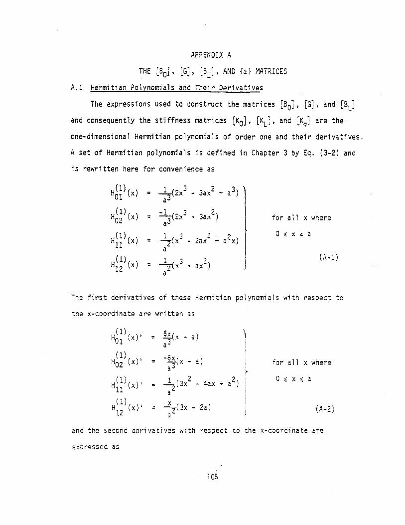
APPENDIX ,A.
THE [So], [G], [BLJ, AND {a} MATRICES
A.I Hermitian Polynomials and Their Derivatives
The expressions used to construct the matrices [80J, [G], and [BLJ
and consequently the stiffness matrices [KO] , [KLJ, and [KcrJ are the
one-dimensional Hermitian polynomials of order one and their derivatives.
A set of Hermitian polynomials is defined in Chapter 3 by Eq. (3-2) and
is rewritten here for convenience as
1 3 2 2-=z<x - 2ax + a x)
a132
Z(x - ax )a
(1)HOI (x) =
H~~)(X) =
H(l)(x) =11
Hg)(X) =
1 3-(2x -a3
-1 3-(2x -a3
3.X: + .3) 13ax ) i for all x where
o ~ x ~ a
(A-I)
The first de~ivatives of these Hermitian polynomials with respect to
the x-coordinate are written as
Hg) (x) I = ~(x - a),
a3 iI
(1) !-6x(x - a) IH
02(x) I = Ia3 I
~
Hii)(x)'1 2 a2)
II
= ~(3x - 4ax + Ia- I
H(l)( )1 = ~(3x - 2a) I12 x a )
for all x where
o ~ x ~ a
(A-2)
and the second derivatives with respect to the x-coordinate are
expressed as
105

106
H(l) ( )" = L(2x - a)01 x a3
H(l)(x)" = -L(2x - a)02 a3
H~~)(X)IIfor all x where
1 4a)= :-r(6x -a o ~ x ~ a
Hg) (x) II1= -=z<6x - 2a) (A-3)a
A.2 Formulation of the [Bo]~[G]__, [BL] and {a} Matrices for the ComputerProgram
To formulate the stiffness matrices of the flat rectangular bend
ing membrane plate element shown in Fig. 3.1 for coding in the computer
program, the nodal displacements at each node of the element are arranged
in the sequence u, ux' uy ' uxY ' v, vx' vy ' vxy ' w, wx' wy ' and wxy ' This
1eads to rearrangi ng the elements of the [BoJ, [GJ, [BLJ, and {cd matri ces
such that the membrane and bending components are separated at each
node. Thus those matrices are written in a partitioned form for each
element as follows:
Eq. (3-29) is written in a partitioned form as
(A-4)
where rB 1 IS 1 rS l and is 1 are r,6x121 submatri ces eXDress-L OllJ' - 012 j
' - 022~' L 021 j- - .
ing the derivatives of the shape functions associated with nodes (1,1),
(1,2), (2,2), and (2,1) respectively. ~atural iy,

107
and {~21} are the vector matrices expressing the corresponding displace
ment parameters. Forms of these matrices are shown in Tables A.I
through A.4.
Simi larly, the [ G ] and [ SL ] matrices are partitioned as
[ G ] = [ [GU ] [G1Z
] [GZZJ [G21
] ] (A-S)
and
[B ] = [ [BLlI
] [B~12J [BL22] [B L21J 1 (A-6)L ..
respectively. Forms of the matrices [Gll] , [G1ZJ, [G22
J, and [G 21J are
shown in Tables A.S through A.8 while forms of the matrices [Slll]'
[BL12
] , [BL22], and [BL21
J are shown in Tables A.9 through A.12.

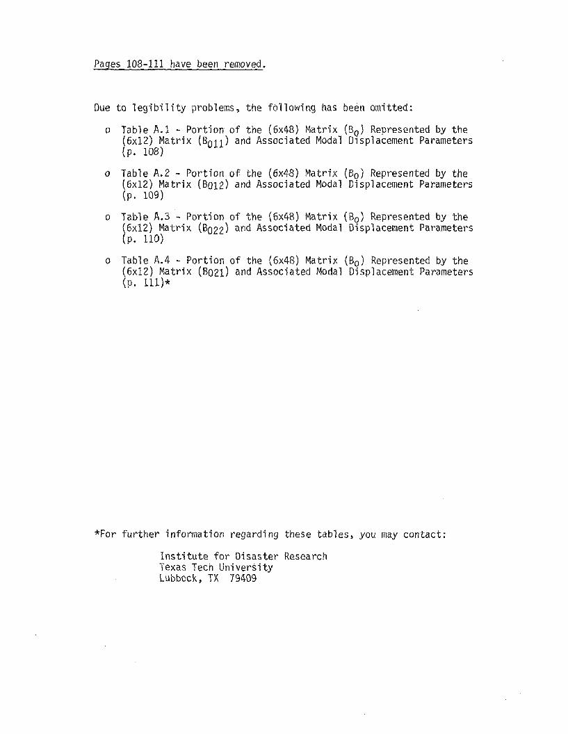
Pages 108-111 have been removed.
Due to legibility problems, the following has been omitted:
o Table A.I - Portion of the (6x48) Matrix (Bo) Represented by the(6x12) Matrix (BOll) and Associated Modal Displacement Parameters(p. 108)
o Table A.2 - Portion of the (6x48) Matrix (Bo) Represented by the(6x12) Matrix (8012) and Associated Modal Displacement Parameters(p. 109)
o Table A.3 - Portion of the (6x48) Matrix (Bo) Represented by the(6x12) Matrix (B022) and Associated Modal Displacement Parameters(p. 110)
o Table A.4 - Portion of the (6x48) Matrix (Bo) Represented by the(6x12) Matrix (B021) and Associated Modal Displacement Parameters(p. 111)*
*For further information regarding these tables, you may contact:
Institute for Disaster ResearchTexas Tech UniversityLUbbock, TX 79409

Table A.5 Portion of the (2x48J Matrix [G] Represented by the (2x12] Matrix [G11
]._.--._-_..._._~- ..--~ --.-1------- - -.-o JO 10 10 10 0 0 0 1I(1)(x)'J1(l)(y) lI(l)(x)'II(1)(y) u(l)(x)'H(t)(y)
01 01 11· 01 01 11-- ._---.~ _ .. __._- '----- -~ ----_. -.- --- -_._-------- ------------(1) (1) '(1) (1) , (1). (1) . '
010 I () 10 10 0 0 0 Jl Ol (x)1I 01 (y) 1111
(x)HOl
(y) HOI (x)lIi1
(y)____.• .. -'__..L---...I • • •
(1) '(1)11 11 (x) JIll (y)
II ( 1 ) ( x )11 ( 1 ) (y ) ,11. 1.1'
Table A.6 Portion of the [2x48J Matrix (G] Represented by the [2x12] Matrix [GI2]
-_.__._-..------.-" . ..---
() 10 10 10 10 10 10 10--·--····-1--+--1--
010 10 10 10 10 10 10
11(1 )(x) 'JIU ley) II ~ ~ ) ( x ) 'II~~ ) ( .Y ) 11(1 lex) 'H(l ley) u(I)(x) '11(1 ley)01 02 01 12 11 12
- -J1(l)(x)II(t)(y) , J1(l)(x)II(1.)(y)' II (1 ) (x)1I ( 1 ) (y) • (1) (l) ,
01 02 11 02 01 12 11 11 (x)1l12
(y)-- --------- -_._._--_.. --
........N
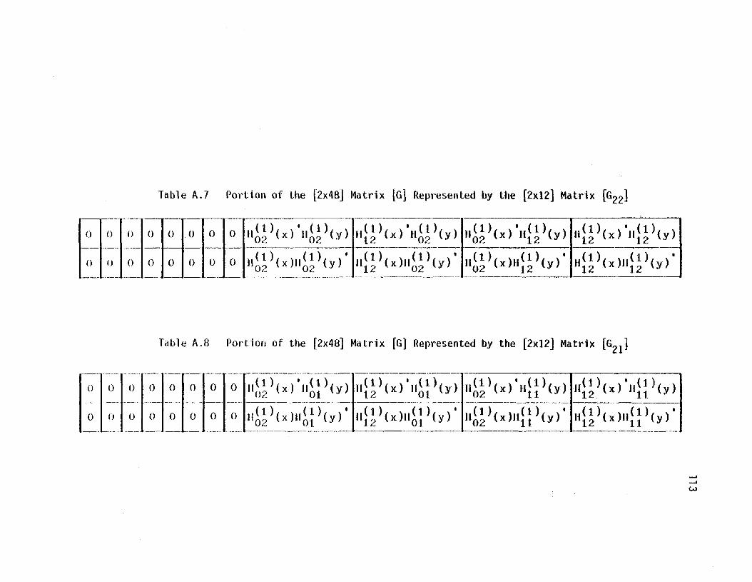
Table A.7 Portion of the [2x48] Matrix [G] Represented by the [2x12] Matrix [G22]
o 10 I (
010
0 0 0 0 0 1I(1)(x) '1I(l)(y) 1l(1)(x) \,(1)(y) JI( 1 )(x) 'II( 1 )(y) H(1 )(x) 'JI(1 )(y)02 02 12 02 02 12 12 12
- - - - -- --------- ----------- -- --0 0 0 0 0 JI{t )(x)JI{t )(y)' Il}~) (x )1I~~) (y) , JI(1 )(x)lI(l )(y)' u(1)(x)Il(1)(y)'
02 02 02 12 12 12·- --- -- --_. ------------------_._- - -
Table A.B Portion of the [2x4B] Matrix [G] Represented by the [2x12] Matrix (G21 ]
010101010101010
010101010101010
. _._...._-------------_. _.---------_._------ ----(1) '(1» lI(l)(x)'H(l)(y) 1l(1 )(x) 'H(1)(y) H(1 )(x) '11(1 )(y)" 02 (x) H01 (y 12 01 02 11 12 11
------------_.. --------- -----II ( 1 ) (x )11 ( 1 ) (y) , II (t ) (x )11 (t ) ( y ) , 1I(l )(x)lI(l )(y)' u(1)(x)JI(1)(y)'
02 01 12 01 02 11 12 11---
--'--'w

Table A.9 Portion of the [6x48] Matrix [Bl ] Represented by the [6x1,2]Matrix (Blli ] and Associated Nodal Displacement Parameters
._-_._----------._--------- ~
(l>W/Z>X) (ow/z,x)
JI(t)(x)'u(1)(y) u(l)(x)'u(l )(y)01· 11 11 11
. --------------(vw/oy) (i)w/c>y)'
11(1 )(x)II(1 )(y)' H(l )(x)Il(1 )(y)'01 11 . 11 11--_._..._-------" -'--
(;:,w/lJY) (c:>w/C>.Y)
Il(l )(x) ')1(1 )(y) H(1 )(x) '11(1 )(y)01 11 11 11
-I- +(e> w/e>x) (i:) w/~ K)
1I(1)(x)H(l)(y)' lI(l)(x)ll(l)(y)'01 . 11 11 11
0101010101010
0101010101010
o 10 10 10 10 10 10
-oro 1(l---lo- r6-ro-ro·-·-~o-T6-·-1-6--1 {)-To·-I 0 10
o 10 10 10 10 10 10
------_.-----_._--_. -----(l)w/()x) (ZJw/ox)
11 0 )(x) ',,(1 )(y) 1I(1 )(x) '11(1 )(y)01 01 11 . 01 .
..._--------_.. --------------(c>W/DY) (Z>w/lJY)
II (l ) ( x )11 ( 1 ) (y ) , 1I(1)(x)H(1 )<.y) ,01 01.' 11 01
• -_· __• ___0._____._- _ ••________•_.~-_.. _._-~._.__._---
(lJ w/lJ.Y ) (aw/z,y)
nO )(x) '11(1 )(y) 1I(t)(x)'II(l)(y)01 01' 11 01'
-I- +(DW/Z,X) (1)w/o x)
u(l)(x)JJ(t)(y)' H( 1 ) (x )]( (1 ) ( y) ,01 01' 11 01'
- ..----------- ...-._-_.__.---- - ._-_._--_.__.~. __ .•._._~
0 0- --------------.._-. ._-------
0 0
0 0'---
oo
oI
o
o --I
__·_·4 __.•..•_~ ~----••_.-f-~-----.---------.-- --------~-- ---]--.------- --'I -I ,- ; ~- • 1
." ::1 :-11 1o~1"-'1:-:: ~: :,. d ~~:' :--~ 1~]'d ~': :-, :xl .-I N :» }-..-I N ~ ~
;1 ;~ ; i:1 :> :> v- v-;:: ~ ~ ~.~---- ~--- -- --- -- -- _.--- -------------------- ------------ ------- -----: :::
.po
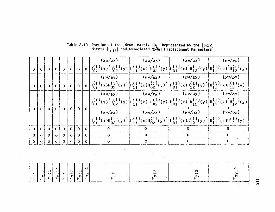
Table A.lO Portion _of the [6x48] Matrix [Bd Represented by the [6x12]Matrix [BL12 ) and Associated Nodal Displacement Parameters
----"- ---------'----.------------- ----_._._-.--- ----(~w/zl)d (bW/3X) «()w/ox) (ow/ax)
o 10 1 () 10101 0 1 0 ) 0111(1 lex) '11(1 ley) 11(_1 lex) '11(1 ley) 11(1 lex) 'H(t ley) 11(1 lex) '11(1 ley)01 02 11 02 01 12 11 12
----- _._-- -- ----- --_. ----------------------------- --------------- ------(l1W/aY) (bW/l>Y) (aw/oy) (?;)w/lJY)
0101°10) 01 0 1 0 ) 011l(l)(x)J1(l)(y)' lI(l)(X)H(1)(y)' lI(l)(x)lI(l)(y)' lI(l)(x)lI(l)(y)'01 - 02' 11 02 01 12 11 12________ . . .. ._.. __M_______ _
(ow/oY) (aw/c>y) (1)w/l)y) (~w/i}Y)
(1) '(1) (1) '(1) (1)' (1) (1)' (1)11
01(x) H
02(y) 11
11(x) 11
02(y) 11
01(x) H
12(y) 11
11(x) "
12(y)
0101010101010101 I- -I- -t- +(ow/ox) <-ow/ax) (aw/ox) (c>w/Z>x)
H~~)(X)II~~)(Y)' lIi~)(X)J1~~)(Y)' 1I~~)(X)lIi~)(y)' Jl11)(X)Jli~)(y)'
~E .. -~;:~~~- -~- .. ~r~~~~~~::~--~ -~-- --::--r-------- ---. ~ -. ~ 1
-_.._..."_.._-.~.-.'--_ ..---.---...---.--------------- --------1:
{\J
T-t~~1
~,J,I~~:f ~.~J ~"J--~j. ; i----·-·_~ ··-·f--------~----I---~1 ~1 ;1 ;:.1 l> l> l> l> ~ ~_________ --- ---- - . -._~ --------------1------
-~Dl-~~ -
;i: .. ~
~
U1
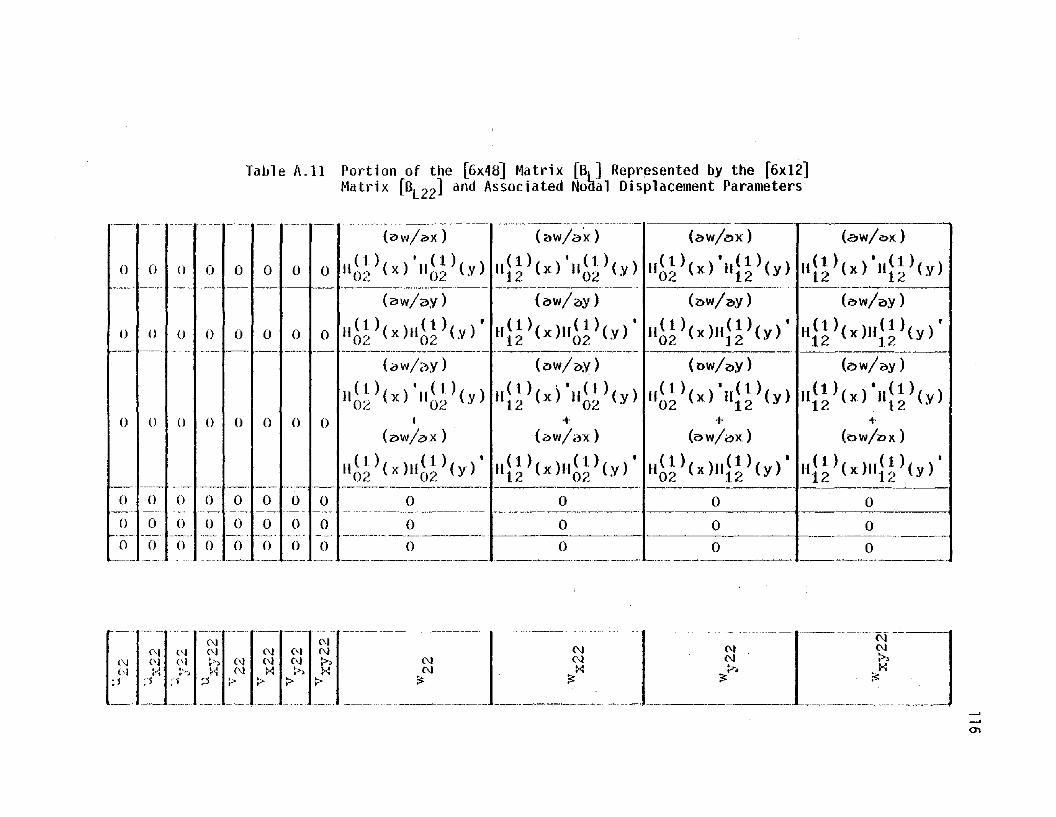
Table A.ll Portion of the [6x48] Matrix [Btl Repr~sented by the [6x12]Matrix [BL22] and Associated Noaal Displacement Parameters
_A . _
o
__ .1--__0
°
o
°o
(21W/C:»X) (aw/ox)
,(l)(x)'I1(l)(y) u(l)(x)'II(t)(y)02 . 12 12 12--_.__._--_.... _----_.__._- ..
('<}w/aY) (bW/oY)
1( 1 ) (x )H ( 1 ) (y )' H( 1 ) (x »)1 (1 ) (y ) ,02 12 12 12
----- -+-- '---- -~--
(l>w/~y) (ow/oy)
,(I )(x) ')(1 )(y) 11(1 )(x) '11(1 )(y)02 12 12· 12
+ +(c>w/2)x) (OW/l> X )
(1) (1) '.(1) (1) •'02 (x)J112 (y) )(12 (x)H12 (y)
." -----_._----------------- ----------_..----_._-_. __...-(<?W/bX) (ow/oid
(1) I (1) 11(1 )(x) '11(1 )(;y)1l0~~ (x) 11 02 (y) 12 02'. ..__._---_._.__._.._-._--
----~_.__._--_.._._._, ..(21w/oY) (.::>w/z,y)
11(1 )(x)II(1 )(y)' H(1)(x)H(1)(y)'02 02' 12 02'
.- ---_.----,----"--_.- -" - ---~,---------,- -
(aw/oy) (~W/bY )
11(1 )(x) '11(1 )(y) (1) ., (1)02 02'
1112
(x) 1102
(y)
I +(z,w/ox) (aw/ax)
11(1 )(x)1I(1 )(y)' II (1 ) (x)1I ( 1) (y) ,02 02 12 02'
- --_._--------- --------_.-_._~-0 0
.__ .... - --._.. ---....---- ->._--------. ,--- -_..._--_._--- ----_._-------_.-- -0 0
-_.".-.--.-._-_._.-------_._------."- . ---------------, _.() 0
----------_.---- ._----.--_•..._.---_..-.
010101010101010
010101010101010
010101010101010
~1% .• ~ ..0 0 0 0 0
0 0 0 0 0
0 0 () 0 0
k;~l~~ ~:~ ?:} ?~ ~~~~_~~~~~I_~~~ __}~~~ _ <'1<'1~.~
--_.. N---.-j<'1:>.l{
;?;
..._---_._---_.~-.............Ol

Table A.12 Portion of the [6x48] Matrix [all Represented by the [6xI2]Matrix [Bl21 ] and Associated Noijal Displacement Parameters
010101010101010
010101010101010
010101010101010
010101010101010
--0-1 () ril- ro' ror-o-rofo010101010101010
- ••••_____ 0 ___ • _ ~_., .•_., _________'.__• ___• .._---,--.._-,---"-_..-._ ..,.- ..-.---(ZJw/c>x) (-cW/ZlX)
11(1 )(x) '}(l )(y) Jj(l)(x)'}(l)(y)02 01' 12 01
..._---_. --_.__._-----_._--_.-.. ---.- .._--- ..". --'-'---'--.'-- .',.
(ow/?JY) (~W/3'y )
II ( ~ ) ( x )11 ( 1 ) (y ) , 1I(1)(x)Jl(t)(y)'Ot:. 01 12 01
. '-- .. _.. " . ----_._.__ ._-_.__...
(lJw/i'Jy) (ow/oY)
11(1 )(x) 'J1<t )(y) lI(l)(x) 'l1(l)(y)02· 01 12 01
+ ..-(ow/ox) (c?>w/"x)
II(!, )(x)H(l )(y) ~ 11(1. )(x)J1(l )(y)'Oc 01 12 01'
. -. ---_._------------- --------_._- -
0 0--_. ------.-. _.•..----------_.__ .__... -. .---,,-- -------~_._.-
0 0-_._--------'-_._------.--. --_._-'--- ..._------------ -'---.
0 0.. . ,._----- ~_._. _...-.. ---- ..__ .._----~_.- _._._---_._-~-_. ~ ..--_._--,-
-------------.-------_.(ow/ax) (aw/3x)
II(~ )(x) ')(1 )(y) H(l )(x) '1\(1 >(y)02 11 12 11
.---------- -'--'~--'.'--_.. -_ .. -_.-- ~-*._--
(ow/~y) (aw/ay)
II ( 1 ) ( x)1I ( 1 ) (y)' II ( 1 ) (x )11 ( i )(y) ,02 . 11 12 11
_..__._._~-- -. ----------_.(ow/oy) (OW/bY)
11(1 )(x) '1I(1 ley) 11(1 )(x) 'n(l )(y)02 11 12 11
+ ..-(aw/?>x) (bIN/oX)
1I(1)(x)H(l)(y)' U(1)(x)lI(l)(y)'02 11 12 11-_.
o 0-- - -----_.._-
o 0~--------
o 0
r----'-- ---- ----1-----~-- 1-' l -----1 [-------J..-1 ..-1 . ,-i
,I ,I (\) , I ..- I (\) , I ..-1 (\) ,
_:}.~: :~~ ~~:_ :.1~__:_!!_ ~:__:: ){ ~~ ~~';1____ __ f<~ _. _ }' __ . ~
~
......

Appendix 8. The [KO] and [KLJ Stiffness Matrices
118

(8-1)
APPENDIX B
iHE [KO] AND [KLJ SiIFFNESS MATRICES
8_.1 Formul ati on of the l[KOL...=...JKLJJ Sti ffness Matri ces for the ComputerProgram
The first term on the right side of Eq. (3-22) in Chapter 3 defines
the sum of the matrices [KO] and [KL] as
r[KO] + [K
L] = I [8] T[0*] [8 ] dV
Jv
Following the nodal numbering scheme atlopted in Appendix A, Eq. (B-1)
can be written as
= JV
(B-2)
The right side of Eq. (B-2) yields a [48x48] matrix which is partitioned
into 16 r12x121 submatrices; for example, the first submatrix is~ ..
r [811JT[O*J [811J dVJ
V
(B-3)
'.vhere [BllJ is a [6x12] matrix \vhich is the sum of [8011J and [BUll'
119

120
For clarity, separate expressions for the elements of portions of
the stiffness matrices [Ko] and [~J as defined by Eq. (8-3) are shown
in sections 8.2 and B.3, respectively.
8.2 Expressions for the Elements of Portion of the Stiffness Matrix [KO]
The following are expressions for the elements of portion of the
stiffness matrix [Ka]. It should be noted that the numbers in parenthesis
indicate the position of that element in the stiffness matrix; for
example, KO(Ol,Ol) is the first stiffness element in the first row and
first column of the stiffness matrix [KoJ.
I-v (1) (1) I
--2-- HOI (x)HOI (Y)

Et J' (1) I (1) (1) (1) I
1-\12 lv HOI (x) HOI (Y)Hn
(X)HOI (y) +
A H(l)( )'H(l)( )' H(l)( )] dA01 Y 11 x 01 \Y
Et ( (1) I (1) (1) (1) I
1-\12 JA
[v HOI (x) HOI (Y)H ll (x)Hll (y) +
H(1 ) ( ) I H(1 ) ( ) I H(I) ( )1 dA01 Y 11 x 11 Y j
I-v (1)T HOI (x)
I-v (1) I
-2- HOI (x-}
I-v (1)-2- HOI (x)
121
Et' f' (1) I (1) 2 1-\) (1) (1) 1 2.I-v2 A[(H ll (x) HOI (y)) + -2-(H ll (x)HOI (y) ) J dA
Et r r (1) I (1) (1) I (1) I-v (1)1-\12 LH 11 (x) HOI (y)HOl (x) Hl1 (y) + --2-- H1l (x)
JA
I (1) I (1) (1) '1HOI (y) HOI (x)H 11 (y) J dA
Et r (1) I 2 (1) (1) . l-\)(H(1)( ))2H
(I)(,)1KO(02,04) = 1-v2 J [(H~l (x) ) HOI (y)Hll (y) 1" 2 11 x 01 Y
A (1) I
Hl1
(y) ] dA
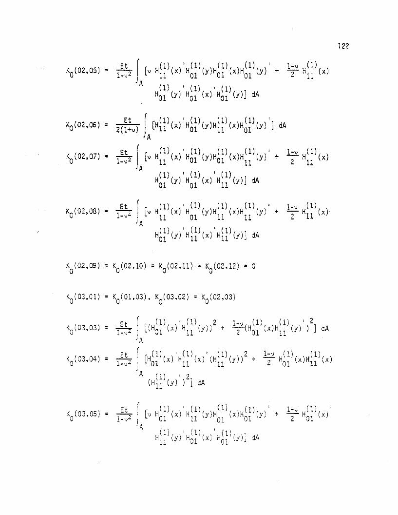
122
KO
(02,OS) =Et r I (1) I (1) (1) (1) I I-v H(1) ( )
1-v2 J [v Hn (x) HOI (y)HOl (X)HOI (y) + 2 11 x
'A (1) I (1) 1(1)Hal (y) HOI (x) Hal (y)J dA
KO(02,06) = Et J (1) '(1) (1) (1) "dA2(l+v) A[H U (x) HOI (y)H n (X)H01 (y) J
KO
(02,07) = ..ll... J [v H(1) (x) ,H(1) ( )H(1) (x1H(1) (y)' • I-v H(l) (x)I-v2 11 01 Y 01 11 2 11
A(1) I (1) I (1) 1
HOI (Y) Hal (x) HI1 (Y)J dA
KO
(02,08) = ..ll,. J [v H(l)(X)'H(1)(')H(1)(X)H(1l( )' • I-v H(l) ( )I-v~ 11 01 Y 11 11 Y 2 11 x
A(1) I (1) J (1) ,
Hal (Y) H11 (x) HU (Y)J dA
C't f r ( 1) I (l) 2 I-v (l) ( 1) I 2KO(03,03) = 1:,)2 ~ L(H01 (x) H
ll(y)) + -2-(H
01(x)H
ll(y) ) ] dA
r\
KO(03,04) = 1~~2 f [Hb~)(X)'Hi~l(X)'(Hi~l(y))2. 1;" Hbil(X)H;i)(x)
A (1) I 2,(HU (y) ) J dA
I-v H(l)( )'2 01 x

I-v (1)2"" HOI (x)
123
K (04,05) =a
K (03 07) Et J [H(l)( )'H(l)( )H(l)( )H(l)( )'1 dAa ' = 2(I+v) 01 x 11 y 01 x 11 Y J
A
K (03 08) -It.. Jr [v H(l)(X)'H(l)( )H(l)(X)H(l)( )' + I-v H(l)(x)a • = I-\)2 01 11 Y 11 11 Y 2 01
A H(l)()'H(l)( )'H(l)( )J dA11 Y 11 x 11 Y
KO
(04,01) = KO
(OI,04), KO
(04,02) = KO
(02,04), KO
(04,03) = KO
(03,04)
Et~ J [(H(l) (x) 'H O) ( ))2 + I-V(H(l) (x\H(l) (\ \ I )2J dAl-v 4 11 11 Y 2 11 IllY/
A
~ r 1- H(l)( )'H(l)( )H(1)( )H(I)( )' + I-v H(l)( )I-v2 LV 11 x 11 Y 01 x 01 Y 2 11 x
'A (1) I (1) 1(1)H11 (y) HOI (x) HOI (y)] dA
I-v (1)()-H x2 11
',KO
(04,07) = Et, r r H(l)(x)IH(l)(Y)H(l)( )H(l)(y)' + 1-') H(l)(X)'l-\)L , LV 11 11 01 x 11 2 11
'A( I' I (1) I (11
H ) f y ' H (x' ~ \ -/ (y. )' dA1 1 , \ ) 1 01 ) "li ~-~ _.

KO
(05,04) = KO
(04,05)
KO(OS,OS) = -S.L J -L(H(1)(X)H(1)(y) 1)2 + 1-v(H(l)(x) ' H(l)(y))21 dAI-v 2 01 01 2 01 01 J
A
(05 06) ...lL r rH ( I) ( )H( I) ( ) (H (1) (1 ) I ) 2... 1·\) H(1) ( ) I (l) I ) I
KO ' = l-v 2 L 01 x 11 x I 01 Y '"2 01 x Hll \x·)A
(H (l ) (y) )21dA01
124
(-\1-\) 1) I
-2- Hal (x)

125
.-S.L J [(H (l ) ( )) 2H( 1) ( ) I H(1) ( ) I +1-~2 11 X 01 Y 11 Y
AH(1) (y )H( 1) (y )J dA
01 11
Et r (1) (1) I 2 I-v (1) I (1) 2.,KO(O? ,07) = 1-\12 [(HOI (x)Hll (y) ) + -2-(H01 (x) H
ll(y)) J cA
I'A
KO
(0?,08) = Et I .'H(l) ( )H(l)( )(H(l)(, )1)2 + l-'J H(l)( )' H(l)( )'1-\12 L 01 x '11 x 11 y 2 '01 x 11 x
A( 1) 2.
(H ll (y)) j dA
K~(08,04) = KO
(04,08), K (08,05) = Kn (05,08), KO(08,06) = KO
(06,08),u 0 u

KO(08,07) = KO
(07,08)
K (08,08) = ..lL Jr [(H(l)(X)H(l)(y) 1)2 + l-\)(H(l)( ) ,H(l)( ))2, dAa 1-\)2 11 11 2 11 x 11 Y JA
126
r ( 1) 11 2, (1) \ (1) j 1) II, (l ) \i (H
O• (x) ) HO•
1(y;H-11 (y) + ') i1
01(x) H (y i
• 1 'J... 01

127
(l ) (l) II (1 ) (l) II (l) II
HOI (X)Hll
(y) + v HOI (X)HOI
(y) HOI (x)
(1) (1) 2 (1) II (1) "Hll (y) + (HOI (x)) HOI (y) Hll (y) + 2(1-v)
H;~)(X)IH~~)(X)I(H~~)(y))2] dA
KO
(09,12) = Et4 J [H(l)(X)I H(l)(Y)H(1)(x)" H(l)(y) + \J H(l)(X)lI
12(I-v2 ) 01 01 11 11 01A
H~~)(Y)H~~)(X)H~~)(y)1I + V H~~)(X)H~~)(Y)"
H(I)(x)"H(I)(y) + H(I)(X)H(l)(y)" H(l)(X)H(l)(y)"11 11 01 01 11 11
(1) I (1) 1 (1) I (1) I
+ 2(1- \J ) HOI (x ) HOI (y) H11 (x) H11 (y) J dA

128
(1) II (1) (1) (1) II (1) (1) II
HOI (x) HI1 (y) + H11 (x)HOl (y) HOI (x)H11 (y)
+ 2(1- )H(l)( )'H(1)( )'H(l)( )'H(1)( )', dAv 11 x 01 Y 01 Y 11 Y J
,
)1 [ (H(1) ( )" H( 1) (\ ) )2 + 2 H(l ) ( ) I' H(1) (1 )H(1) ( )
01 x 11 Y J v 01 x 01 YJ 1 01 xA
(1) II + (1) (1) 1 II 2.. _ (1)/ I
HU
(y) (HOI (x)HU
(y)) ,2(1 ,J)(H01
\x)
Hi~) (y) I ) 2] dA
( (I) "(I'" () 2 (1) 11(1)I [Hal (x) H1/ (x) (H 1i (y)) .. 'J HO~ (x) H~i (y)
JA( 1 ) ( i ) 'I ( i ) ( • \ II ('1' II
H - ()H - (\1' "-, H'" ()H 1)( ) H'·)()'11 x 11 jJ J 01 x"n \Y '11 x
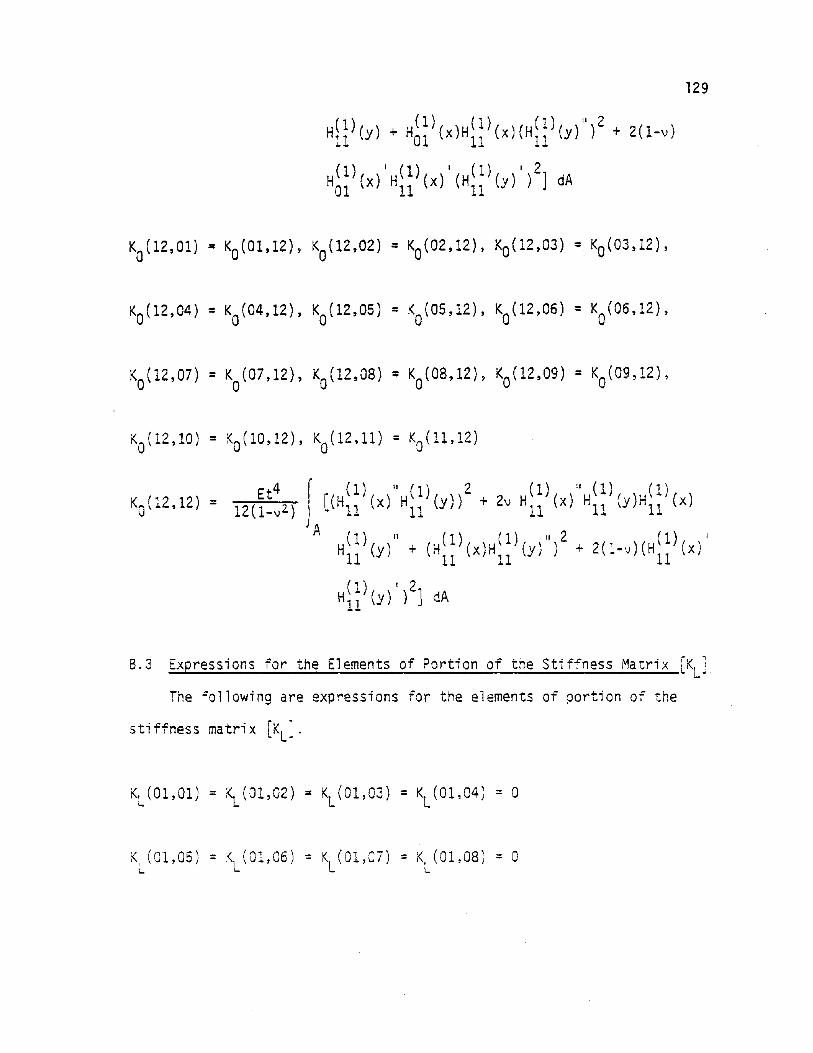
129
Hg)(Y) + Hg)(X)Hg)(X)(Hg)(y)")2 + 2(l-v)
H(l) (x) I H(l) (x) I (H (l ) (y) I )2] dA
01 11 11
B.3 Expressions for the Elements of Portion of the Stiffness Matrix rK 1.. L"
The following are expressions for the elements of portion of the
stiffness matrix [KL].

(01 09) ..n.. ( [ aW1H(1)( )' H(1)( ))2 + (h) oW H(l)( )H(1) (_I )'Kl ' = I-v2 ) ~ 01 x 01 y 2 3y 01 x 01 y
'AH(l) ( ) I H(l) ( ) + (h) ali~ (H(l) ( )H(1)( ) I )2] dA
01 x 01 y 2 ax 01 x 01 y
K (01,10) = .J..L If [~H(l)( )'H(l)( )'(H(l)( ))2 + aw H(l)( )1L I-v2 ax 01 x 11 x 01 y v 3y 01 x
'AH(1)(Y)H(1)(X)H(1)(y)' + (l-v)(~ H(I)(X)H(I)(y) 1
01 11 01 2 ay 01 01
H(l) (x) I H(l) (y) + aw H(l) (x) H(l) (x)( H(l) (y) I )2) ] dA
11 01 ax 01 11 01

131
KL
(02,10) = ...!.L f [~H(l)(X)'H(l)( ))2 + (l+'J) ~ H(l)(X)'H(l)(..)I-v2 ax' 11 01 Y 2 ay 11 01 Y
A H(1) ( )H(l) ( ) I + (1- v) (H ( 1) ( )H(1) ( ) I ) 2 3w 1 dA11 x 01 y 2 11 x 01 Y ax J
KL(03,01) = KL(03,02) = KL
(03,03) = KL
(03,04) = 0
KL(03,05) = KL
(03,06) = KL
(03,07) = KL
(03,08) =°
'K (n3 09) - EtI L 'oJ, - 1-\)2
.~ oW , (l) I 2 (1) (l) , 3W"( 1) f ,,(l )L :-(H (x)) HI' (y)H01 (Y) .,.. 'J "\ H01 \x) H'1 (y).x 01 .'J. ....l.
A (1) (1' I (1) (1' (')H ( \H .. ) (\ .;., (1- \)) (,w ... r,), ) (, ' " :.. ( \ II X;I 'I), ~ "HOI ,,< H.
1,y) H \x)
01 01 oJ '::::;1 1- 01

132
KL
(04,01) = KL
(04,02) = KL(04,03) = KL
(04,04) = 0
\ (04,09) = ~ r r oW (l) ( ) I (l) (\) (1) ( ) I I (l) ( ) + oW I (l) ( ) I
2 , l - H X H Y H X H Y v -~ H1I
XI-v ax 11 11 01 01 ~y
JAH(l)( )H(l)(X)H(l)(I)' + (l-v\( jW H(l)(X)H(l)(I)'
1, y 01 i"'l Y '? 1 '1· 11 Y~ u _?y 1 __
( '\ I (.) '(" (I' I 11\1 J () 1 I) ~W ... ) ( )' J ( ) U\ 1 { \
HOI x HOI ,Y ... - H1 X H Y "J1 \Xl·,x _1 11 ; -
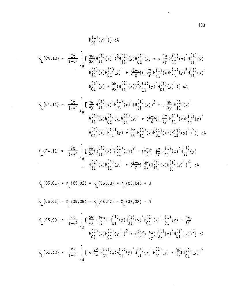
KL
(04, 10) =
K (04,11) =L
K (04,12) =L
133
H6~) (y) I) ] -dA
..lL f [~H(l) (x) I )2H(l) ( )H(l) (, ) + v oW H(l) (x) I H(l) ( )1-v2. J ax 11 11 Y 01 Y ay 11 11 Y
AH(l) (X)H(l) (y) I + (1-v)( aw H(l) (X)H(l) (y) I H(l) (x) I
11 01 2 ay 11 11 11
H(l)(y) + ~(H(1)(x))2H(1)( ) 'H(l)( ) I)] dA01 ax 11 11 Y 01 Y
K1
(05,01) = K (05,02) = KL
(05,03) = K (05,04) = a- L L
KL
(05,05) = KL
(05,06) = KL
(05,07) = KL
(05,08) = 0
K (05,09) =L
:< (05,10) =L
Et-,.,1-')"'"
'W (1) (1\ I (1) I (1) '(11 ?~ 'J ~ H ( x) H\ ) (y) H - (x) H • (y) -:- ~w (H / (y. \ \ -
;x 01 \ 01 11 01 ~y\ 01 \ IJ

1341
KL(06,01) = KL
(06,02) = KL
(06,03) = KL
(06,04) = a
K (06,05) = K (06,06) = K (06,07) = KL
(06,08) = aL L L
Et I ,-3 W( 1+') ) (l ) ( \ (l). ) I (1 ) ( ) I (l) (\ :; WI (l) (K, (86,10) = -1-, i -, - H x)HUH x HO
y) + -,\ H xL _\)L i ~ -:ox 2 11 01 11 1 dy 11
j A
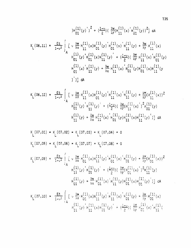
135
I
) )J dA
K (07,01) : K (07,02) : K (07,03) = K (07,04) = 0L L L L
KL(07,05) = KL
(07,06) : KL(07,07) = KL(07,08) : °
(07 09) Et I( [" oW H(l) ( )H(l) (. ) I H(l) ( ) I H(l) ( ) + 3W(H(l) ( ))2KL ' : I-v2 l v ax 01 x 11 Y 01 x '01 Y 3y 01 x
JAH(l)(Y)'H(l)(y)' + (1-\))( aW(H(I)(x)')2H(l)(y\
11 01 2 3Y 01 11 I
H(l ) ( ) + oW H( 1) (x) I H(l) (y) H(l ) (x) H( 1) (y) I )' dA01 y ax 01 11 01 01 J

136
I
y) )J dA
KL(08,01) = KL
(08,02) = KL
(08,03) = KL
(08,04) = 0
KL
(08,05) = KL(08,06) = KL(08,07) = KL
(08,08) =°
\ (08,09) =Et r ~ oW (1) (1) I (1) 1(1) dW (1)
1-\J2 I L v oX H11 (x)H ll (y) HOI (x) HOI (y) +;y Hll (x)J
A H(1) ( ) I H(l ) (x) H(l ) ( ) I + ( l-'J ) ( ;W H( 1) ( I I H( 1) ( )I 11 Y 01 01 Y 2,Y 11 x I 11 \y
(1) I (1\ 3w (1) I (1) (1) (1) I
H (x) H • J (y) + - H (x) H (y) H (x) H - (y \01 \ 01 ax 11 11 01 01 I
)] dA
K (08,10) =L
Et1-\)2

H(1) ( ) + aw H(1) ( ) I H(l ) ( )H(1) ( )H(1) ( ) I ) 1 dA01 y ax 11 x 11 y 11 x. 01 Y j
137
K (09,01) = K (01,09), K (09,02) =K (02,09), KL
(09,03) =KL
(03,09),L L L L
KL
(09,04) = KL
(04,09), KL
(09,05) = KL
(05,09), KL
(09,06) = KL
(06,09),
K (09,07) = K (07,09), K (09,08) = KL
(08,09)l L L
\ (09,09) =

KL(09,lO) =
K (09,11) =L
138
K (10,01) = K (01,10), K (10,02) = KL
(02,10), :< (10,03) = K, (03,10),L l l L L
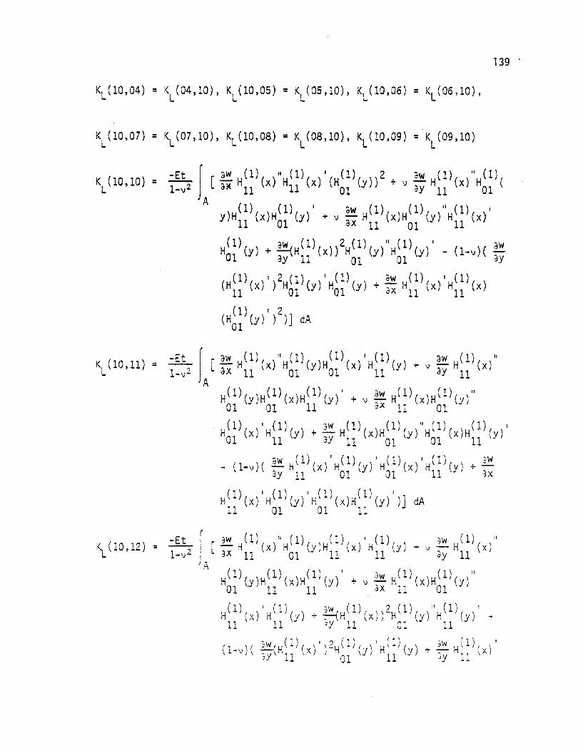
K (10,10) =L
139 .
KL(10,07) = KL(07,10), KL(10,08) = K
L(08,10), K
L(10,09) = K
L(09,10)
:ILJ [~w H(1)(X)II H(l)(X)I(H(l)( ))2 + \) dW H(l)(X)"H(l\1-v2 a* 11 11 01 Y ay 11 01
A)H(1) (x) H(l ) ( ) I + V aw H(l) (x) H(l) (\ )II H(l) (x) I
Y 11 01 y ax 11 01 y 11
H(l)( ) + ~H(I)(x))2H(l)( )II H(l)( )' _ 'l-v)( aw01 y ay 11 01 y 01 y \ ay
(H(l)( )')2H(1)( )' H(l)( ) + aw H(I)( )' H(I)( )11 x 01 Y 01 y 3X '11 x 11 x
(H~ ~) (y) I )
2) j dA
\ (10,12) = -Et r r aw H(l) ( )"H(l) ( )H(l) ( ) I ,J1) ( ) jW H( 1) ( )"- I ' - I X Y X i1 Y + \) - X1-\)2 I L ax 11 01 11 11 ay 11
JAH( 1) ( )H(l) (x) H(l) (\ ) I + \) 3w H( 1) (x) H( 1) (y) "
01 y 11 11 y ax 11 01
H( 1) ( ) I H(l ) (.) , jW (u (l ) ( \) 2H( 1) ( )"., (l ) ( ) I
I X I y'" -," XI Y H Y -11 11 Jy 11 01· 11 \
, ( 1 ) I 2 (, \ I (1) 'W,' i ) I('_,)f JW'H .. ( ) \ H\.l.) (, \ H - (\ \ + .::.- H\- fv\\J.) \ ;y"ll ,X) '01 )/ '11 YJ 3y 11 ,Ai
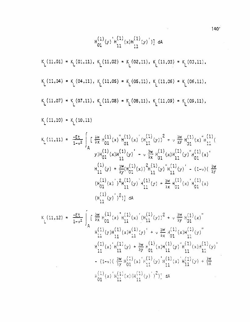
K (11,01) = KL(Ol,ll), K (11,02) = K (02,11), K (11,03) = K (03,11),L L L L L
KL(11,04) =K (04,11), K (11,05) =KL
(05,11), K (11,06) = K (06,11),L L L L
140'
K (11,12) =L

141
K (12,01) = K (01,12), K (12,02) = KL
(02,12), K (12,03) = K (03,12),L L L L L
K (12,04) = KL
(04,12), K (12,05) = K (05,12), K (12,06) = K (06,12),L L L L L
KL{12,10) = KL
(10,12), ~(12,11) = KL
(11,12)
K (12 12) -Et j( r ~w H(1){x)Il H(1)(x)' (H{l){ ))2 + \) oW H(1)(x,"H(I)(I L ' = I-\)2 I. oX 11 11 11 y ?Jy 11 I. 11
A)H(1) (x) H(1) (' ) I + 'J :w H(l) (x) H(l) ( ) 11 H(1) (x) I
Y 11 11 y oX 11 11 Y 11
(l) 3w (1) 2 (1) 11 (1)' 3wH
11(y) + ~Hl1 (x)) H
ll(y) H
11(y) - (1-\1)( ay
(H(l)(X)')2H(l)( )'H(l)( ) + aw H(I)(X)'H{l)(x)11 11 y 11 Y ax 11 11
(H~~)(y)')2)J dA

Appendix C. The rK 1 Stiffness Matrix- c~
142
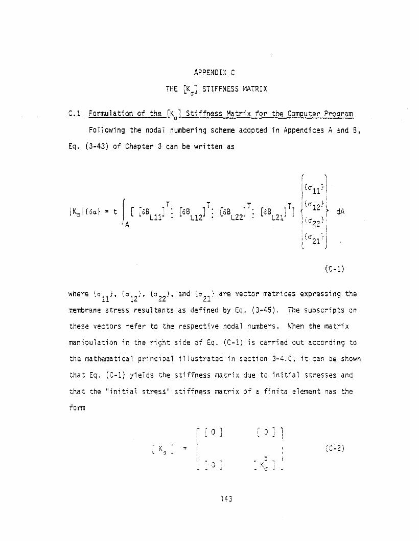
APPENDIX C
THE [K~J STIFFNESS MATRIX~
e.l Formulation of the [Kcr
] Stiffness Matrix for the Comouter Program
Following the nodal numbering scheme adopted in Appendices A and B,
Eq. (3-43) of Chapter 3 can be written as
I K I {' 1 = r [ r·B 1T. Ll'"o' BL12'J T'. [.8 ] T. 1'". B ~ T1I' (11 OCLr t LO LlIJ . 0 LZ2 : LO L21J J
JA
(C-1)
where {all}' {alZ}' {cr22
}, and {a2l
} are vector matrices expressing the
membrane stress resultants as defined by Eq. (3-45). ihe subscripts on
these vectors refer to the respective nodal numbers. When the matrix
manipulation in the right side of Eq. (C-1) is carried out according to
the mathematical principal illustrated in section 3-4.C, it can be shown
that Eq. (C-1) yields the stiffness matrix due to initial stresses and
that the Ilinitial stress" stiffness matrix of a finite element has the
form
K "1 :::
.. ''1''
i 0 J
,i _
o'- '- ~
143
o IJ
b,- K .,- 'iJ ..I

144 .
where
r N N.,I
~ Kb ,(
r G ' TI x xy
I= t i [G ~ dAL cr j
JAL 11J
I U J
N NL
xy y I.J
(C-3)
C.2 Expressions for the Elements of Portion of the Stiffness Matrix [KcrJ
The following are expressions for the elements of portion of the
"initial stress ll stiffness matrix [KcrJ.
K (01,01) = K (01,02) = K (01,03) = K,..,(01,04) = K (01,05) = K (01.06) = 0~ ~ ~ ~ ~ ~
K (02,07) = K (02,08) = K (02,09) = K (02,10) = K (02,11) = K (02,12) = 0cr J a ~ cr v
K (03,01) = K (03,02) = K (03,03) = K (03,04) = K (03,05) = K (03,06) = 0cr cr cr cr cr cr
= K ! ('14 10')-:;'-..1 ,. = 0
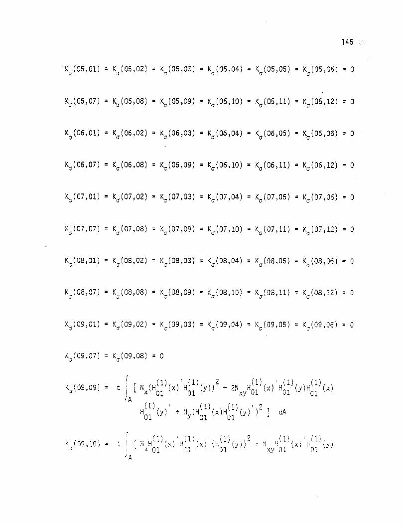
145
K (05,01) = K (05,02) = K (05,03) = K (05,04) = K (05,05) = K (05,06) = 0cr cr cr cr cr cr
K (07,07) = K (07,08) = K (07,09) = K~(07,10) = K~(07,11) = K (07,12) =0cr cr cr v U cr
K (08,01) = K (08,02) = K (08,03) = K~(08,04) = K~(08,05) = K (08,06) =°cr cr cr v U cr
KJ
( 09 ,09) =
K (09,10) = .f.J
A

146
K (10,01) = K (10,02) = K (10,03) = K (10,04) = K (10,05) = K (10,06) = 0cr cr cr v v cr
1/ '10 10') ="J \ - ,-
Kj 10,11) =:..J
( 1) (,\ 1/,\ '1\ Iw - I 'H'-J( , ,,\1'( ,,,I I, \ ' ',~+ N n \ X) , \y):'i " X)H \.Y , ' Of.,
Y 11 01 01 11 -

K (10,12) = • r [N fH(l)(X)')2H(1)( )H(l)( ) + N H(l)(X)'HO(ll)(Y)J l.. I x\ 11 01 Y 11 Y xy 11
JAH( 1) (x \H( 1) (y) I + N H( 1) (x) H( 1) (y) I H( 1) (x) I H( 1) (y)
11 J 11 xy 11 01 11 11
+ N (H(l) Ix) )2H(l) (y)' H(l) (y)' ] dAy 11 \ 01 11
147
K (11,11) =(J
K (11,12) =J
" (120 0 ) - < (1'"'1912) K f,? 10) :< ("0 '2\l"~ \_ ,.., -'.,. u, " ~ \ .1._ , .. = . .,. J. ,.1. ),.... ~ ~ -'
K ( '2 11\ K roo 12)I .,. .I. , ..... ) = ;':J \ ll, ..

148