abap tutorial session 5 internal tablestutor.nmmu.ac.za/norma/wrer302/abap tutorial session 5.pdf1...

1

ABAP Tutorial Session 5

Internal Tables

Chapter Objectives After you complete this chapter, you should be able to:

Define an internal table with or without a header line using the data and include structure

statements.

Fill an internal table by using append via a header line or an explicit work area.

Use loop at and loop at...where to read the contents of an internal table, and use sy-tabix to

determine the current row index.

Locate a single row in an internal table by using read table and its variations.

Sort internal tables and use the as text addition.

Internal Table Basics An internal table is a temporary table stored in RAM on the application server. It is created and filled by a

program during execution and is discarded when the program ends. Like a database table, an internal table

consists of one or more rows with an identical structure, but unlike a database table, it cannot hold data

after the program ends. Use it as temporary storage for manipulating data or as a temporary private buffer.

Definition of an Internal Table

An internal table consists of a body and an optional header line .

The body holds the rows of the internal table. All rows within it have the same structure. The term "internal

table" itself usually refers to the body of the internal table.

The header line is a field string with the same structure as a row of the body, but it can only hold a single

row. It is a buffer used to hold each record before it is added or each record as it is retrieved from the

internal table.

NOTE

In this tutorial, a naming convention is used for internal tables. For simple programs

with only a single internal table, the internal table name will usually be itab (for

internal table). If multiple internal tables exist, the name of each will usually begin

with itab.

To define an internal table body, use occurs n on the definition of any field string except tables. occurs

creates the body of the internal table. The memory for the body is not allocated until the first row is added

to it. Without occurs, you only have a field string.

To define an internal table with a header line, you must include either begin of or with header line in

the definition. A header line is automatically created if begin of appears in the definition. If you use like

instead of begin of, the internal table will not have a header line unless you add with header line after

the occurs clause. This is illustrated in lines 2 through 10 of Listing 7.1.

The only time you would create an internal table without a header line is in the case of a nested internal

table. A nested internal table cannot have a header line.

2

Listing 7.1 Basic Ways of Defining Internal Tables with and Without a Header Line 1 report z##0701.

2 data: begin of itab1 occurs 10, "has a header line

3 f1,

4 f2,

5 f3,

6 end of itab1.

7

8 data itab2 like lfa1 occurs 100. "doesn't have a header line

9

10 data itab3 like lfa1 occurs 100 with header line. "it does now

The code in Listing 7.1 does not produce any output.

Line 2 begins the definition of an internal table named itab1. Itab1 is an internal table because of

the presence of the occurs clause. It has three components: f1, f2, and f3. Each is type c, length 1.

This internal table has a header line because the definition contains the words begin of.

Line 8 defines internal table itab2. It has the same components as the DDIC structure lfa1. It does

not have a header because neither begin of nor with header line appear in the definition.

The definition of itab3 on line 10 is almost the same as the one for itab2 on line 8. The only

difference is the addition with header line. This, of course, causes itab3 to have a header line.

Clearing Up the Main Source of Confusion Surrounding Internal Tables

Figure 7.1 contains a typical internal table definition. It defines two things: the body of an internal table

and a header line. Confusion arises because both the body and the header line are named itab. itab is the

name of the body, and itab is also the name of the header line. Where you place the name itab in your code

determines to what you are referring.

When used in an assignment statement, it always refers to the header line. For example, itab-f1 = 'A'

refers to component f1 of the header line named itab. Or in f3 = itab-f1, the header line itab is also

referred to.

Examples of Internal Table Definitions

To define internal tables with and without header lines, use the forms recommended in Listing 7.2.

Listing 7.2 These Definitions Create Internal Tables with and Without a Header Line 1 report z##0702.

2 data: begin of itab1 occurs 10, "has a header line

3 f1,

4 f2,

5 f3,

6 end of itab1.

7

8 data itab2 like lfa1 occurs 100. "doesn't have a header line

9

10 data itab3 like lfa1 occurs 100 with header line. "it does now

11

12 data itab4 like itab3 occurs 100. "doesn't have a header line

13

14 data begin of itab5 occurs 100. "has a header line

15 include structure lfa1.

16 data end of itab5.

17

18 data begin of itab6 occurs 100. "this is why you might use

19 include structure lfa1. "the include statement

20 data: delflag,

21 rowtotal,

22 end of itab6.

3

23

24 data: begin of itab7 occurs 100, "don't do itab this way

25 s like lfa1, "component names will be

26 end of itab7. "prefixed with itab7-s-

27

28 data itab8 like sy-index occurs 10

29 with header line.

30

31 data: begin of itab9 occurs 10,

32 f1 like sy-index,

33 end of itab9.

The code in Listing 7.2 does not produce any output.

Lines 2 through 10 are the same as those in Listing 7.1; they are included here for your review.

On line 12, itab4 is defined like the field string named itab3, not like the internal table itab3. Thus,

an occurs addition is required to make itab an internal table; this one does not have a header line

because there is no begin of or with header line.

Lines 14 through 16 show the old way of defining an internal table. itab5 is the same as itab3

defined on line 10. The like addition was only introduced in release 3.0; prior programs use

definitions like this one. Include structure is not used now except for cases such as the

following definition of itab6.

This is the only practical reason you would use the include statement now (after release 3). It

enables you to create a field string having all components from a DDIC structure plus some

additional ones. The definition of itab6 contains the components of lfa1 and two additional fields

delflag and rowtotal. This internal table has a header line because you see begin of in the

definition.

Lines 24 through 26 show the wrong way to use like. The components of this internal table all

begin with itab7-s, for example, itab7-s-lifnr and itab7-s-land1. Although it is workable, it is

probably not what was intended, and introduces an unnecessary level into the component names.

When defining an internal table that has a single component, you can use either the declaration on

line 28 or on line 31.

Adding Data to an Internal Table Using the append Statement

To add a single row to an internal table, you can use the append statement. append copies a single row

from any work area and places it in the body at the end of the existing rows. The work area can be the

header line, or it can be any other field string having the same structure as a row in the body.

Syntax for the append Statement

The following is the syntax for the append statement. append [wa to] [initial line to] itab.

where:

wa is the name of a work area.

itab is the name of a previously defined internal table.

The following points apply:

wa must have the same structure as a row of the body.

wa can be the header line or it can be any field string having the same structure as a row in the

body.

If you do not specify a work area, by default the system uses the header line. In effect, the header

line is the default work area.

After append, sy-tabix is set to the relative row number of the row just appended. For example,

after appending the first row, sy-tabix will be set to 1. After appending the second row, sy-tabix

will be 2, and so on.

4

The statement append itab to itab appends the header line named itab to the body named itab. The

statement append itab does the same thing, because the default work area is the header line. Being more

succinct, the latter is usually used.

A work area mentioned explicitly in the append statement is known as an explicit work area. Any field

string having the same structure as a row of the internal table can be used as an explicit work area. If a

work area is not mentioned, the implicit work area (the header line) is used.

The statement append initial line to itab appends a row containing initial values (blanks and zeros)

to the internal table. It is the same as executing the following two statements in succession: clear itab

and append itab.

Listing 7.3 shows a sample program that appends three rows to an internal table.

Listing 7.3 This Program Adds Three Rows to Internal Table itab from the Header Line 1 report z##0703.

2 data: begin of itab occurs 3,

3 f1(1),

4 f2(2),

5 end of itab.

6 itab-f1 = 'A'.

7 itab-f2 = 'XX'.

8 append itab to itab. "appends header line itab to body itab

9 write: / 'sy-tabix =', sy-tabix.

10 itab-f1 = 'B'.

11 itab-f2 = 'YY'.

12 append itab. "same as line 8


14 itab-f1 = 'C'.

15 append itab. "the internal table now contains three rows.


The code in Listing 7.3 produces this output: sy-tabix = 1

sy-tabix = 2

sy-tabix = 3

Line 2 defines an internal table named itab and a header line named itab. Both have two

components: f1 and f2.

Lines 6 and 7 set the contents of header line fields f1 and f2.

Line 8 copies the contents of the header line named itab to the body named itab.

Lines 10 and 11 assign new contents to the components of the header line, overwriting the existing

contents .

Line 12 appends the new contents of the header line to the This statement is functionally equivalent

to the one on line 8. Because a work area is not named, the default work area-the header line-is

used.

Line 14 changes the value of itab-f1 and leaves the in itab-f2 alone .

Line 15 appends a third row from the header line itab to the body itab.

Using the occurs Addition

occurs does not limit the number of rows that can be added to the internal table. For example, if you

specify occurs 10, you can put more than 10 rows into the internal table. The number of rows you can put

into an internal table is theoretically only limited by the amount of virtual memory available on the

application server.

5

The system uses the occurs clause only as a guideline to determine how much memory to allocate. The

first time a row is added to the internal table, enough memory is allocated to hold the number of rows

specified on the occurs clause. If you use that memory up, more is allocated as needed.

Alternatively, you can specify occurs 0. If you do this, the system allocates 8KB pages of memory at a

time. However, there are no advantages to using occurs 0 other than the fact it is only a little easier to

code occurs 0 than it is to estimate the size of the internal table. For peak performance and minimum

wasted memory, choose an occurs value equal to the average maximum number of rows in the table. For

example, if most of the time the internal table is filled with a maximum of 100 rows, but every once in a

while it is filled with a maximum of 1,000 rows, set the occurs value to 100.

Reading Data from an Internal Table

Two statements are commonly used to read the data from an internal table:

loop at

read table

Use loop at to read multiple rows from the internal table. Use read table to read a single row.

Reading Multiple Rows Using the loop at Statement

To read some or all rows from an internal table, you can use the loop at statement. Loop at reads the

contents of the internal table, placing them one at a time into a work area.

Syntax for the loop at Statement

The following is the syntax for the loop at statement.

loop at itab [into wa] [from m] [to n] [where exp].

---

endloop.

where:

itab is the name of an internal table.


m and n are integer literals, constants, or variables representing a relative row number. For

example, 1 means the first row in the table, 2 means the second, and so on.

exp is a logical expression restricting the rows that are read.

--- represents any number of lines of code. These lines are executed once for each row

retrieved from the internal table.

The rows are read from the internal table one at a time and placed in succession into the work area.

The lines of code between the loop at and endloop are executed for each row retrieved. The loop

finishes automatically when the last row has been read, and the statement following the endloop is

then executed.



wa can be the header line or it can be any field string having the same structure as a row in

the body.

If you do not specify a work area, by default the system uses the header line. For example,

loop at itab into itab reads rows from the internal table itab, placing them one at a

time into the header line itab. An equivalent statement is loop at itab.

If from is not specified, the default is to begin reading from the first row.

If to is not specified, the default is to read to the last row.

6

Components of itab specified in the logical expression should not be preceded by the

internal table name. For example, where f1 = 'X' is correct, but where itab-f1 = 'X'

will cause a syntax error.

exp can be any logical expression. However, the first operand of each comparison must be a

component of the internal table. For example, if itab contains a component f1, then where

f1 = 'X' would be correct; where 'X' = f1 would be incorrect and causes a syntax error.

The from, to, and where additions can be mixed at will.

Within the loop, sy-tabix contains the relative row number of the current record. For example,

while processing the first record in the internal table, the value of sy-tabix will be 1. While

processing the second, sy-tabix will be 2. Upon exiting the loop, the value of sy-tabix is reset to

the value it had when the loop began. If loops are nested, the value in sy-tabix relates to the

current loop.

After endloop, sy-subrc will be zero if any rows were read. it will be non-zero if no rows were

read from the internal table.

Listing 7.4 expands on Listing 7.3, looping at and writing out the rows of the internal table.

Listing 7.4 This Program Adds 3 Rows to Internal Table itab from the Header Line, and Then

Writes Them Back out Again 1 report z##0704.


3 f1(1),

4 f2(2),

5 end of itab.

6 itab-f1 = 'A'.

7 itab-f2 = 'XX'.

8 append itab to itab. "appends header line itab to body itab

9 itab-f1 = 'B'.

10 itab-f2 = 'YY'.

11 append itab. "same as line 8

12 itab-f1 = 'C'.

13 append itab. "the internal table now contains three rows.

14 sy-tabix = sy-subrc = 99.

15 loop at itab. "same as: loop at itab into itab

16 write: / sy-tabix, itab-f1, itab-f2.

17 endloop.

18 write: / 'done. sy-tabix =', sy-tabix,

19 / ' sy-subrc =', sy-subrc.

The code in Listing 7.4 produces this output: 1 A XX

2 B YY

3 C YY

done. sy-tabix = 99

sy-subrc = 0

Lines 2 through 13 are the same as those in Listing 7.3. They add three rows to the internal table.

Line 14 sets sy-tabix and sy-subrc to an arbitrary value.

Line 15 begins a loop that reads the first row from the internal table named itab, placing itab into

the header line itab.

Line 16 writes out the value of sy-tabix and values in the components of the header line.

Line 17 marks the end of the loop. itab returns to line 15.

Line 15 is re-executed. This time, the second row from the internal table is placed into the header

line, overwriting the previous contents.

7

Line 16 is executed, again writing out values from the header line.

On line 17, the loop repeats until all rows have been retrieved from the internal table. When the last

row has been read, it stops looping.

On line 18, sy-tabix has been restored to the value it had before the loop was executed. Sy-subrc

contains zero, indicating that rows were retrieved from the internal table by the loop at statement.

Restricting the Rows Read from the Internal Table

Using the from, to, and where additions, you can restrict the number of rows read from the internal

table. Listing 7.5 expands on Listing 7.4, looping at the internal table four times. Each time it writes

out only certain rows.

Listing 7.5 This Program Is Like Listing 7.4, but Only Some of the Rows Are Read 1 report z##0705.


3 f1(1),

4 f2(2),

5 end of itab.

6 itab-f1 = 'A'.

7 itab-f2 = 'XX'.

8 append itab.

9 itab-f1 = 'B'.

10 itab-f2 = 'YY'.

11 append itab.

12 itab-f1 = 'C'.

13 append itab. "it now contains three rows

14

15 loop at itab where f2 = 'YY'. "f2 is right, itab-f2 would be wrong

here


17 endloop.

18 skip.

19

20 loop at itab to 2. "same as: loop at itab from 1 to 2.


22 endloop.

23 skip.

24

25 loop at itab from 2. "same as: loop at itab from 2 to 3.


27 endloop.

28 skip.

29

30 loop at itab from 2 where f1 = 'C'.


32 endloop.

The code in Listing 7.5 produces this output: 2 B YY

3 C YY

1 A XX

2 B YY

2 B YY

3 C YY

3 C YY

Lines 2 through 13 add three rows to the internal table.

8

Lines 15 through 17 read only those rows from the internal table where f2 has a value equal to

'YY'. Only rows 2 and 3 satisfy the criteria.

Line 18 skips a line in the output, in effect writing a blank line.

Lines 20 through 22 read only rows 1 and 2 from the internal table.

Lines 25 through 27 read only rows 2 and 3 from the internal table.

Line 30 reads beginning from row 2, looking for all rows having an f1 value of 'C'. Row 3 is the

only matching row in this range.

CAUTION

Although the where returns a subset of the table contents, a full table scan is always

performed. Caution.

If you make sure the data type and length of the field in exp matches the internal table field exactly, no

conversions will be performed. This causes your loop to run more quickly. If conversion is required, it is

performed on every loop pass and this can slow processing down considerably. Use like or constants to

avoid conversion.

Using exit, continue, stop, and check

Table 7.1 illustrates the effects of exit, continue, and check when used within a loop

at/endloop construct.

Table 7.1 Statements that Can Alter Loop Processing for Internal Tables

Statement Effect

exit Terminates the loop immediately. Processing continues at the statement

immediately following endloop.

Continue

Goes immediately to the endloop statement, bypassing all following

statements within the loop. The next row is returned from the internal

table and processing continues from the top of the loop. If there are no

more rows to retrieve, processing continues at the first statement

following endloop.

Check exp If exp is true, processing continues as if this statement had not been

executed. If exp is false, its effect is the same as continue.

Reading a Single Row Using the read table Statement

To locate and read a single row from an internal table, use read table. It reads a single row that matches

specific criteria and places itab in a work area.

Syntax for the read table Statement

The following is the syntax for the read table statement.

read table itab [into wa] [index i | with key keyexp [binary search] ]

[comparing cmpexp] [transporting texp].

where:



i is an integer literal, constant, or variable representing a relative row number. For example,

1 means the first row in the table, 2 means the second, and so on.

keyexp is an expression representing a value to be found.

cmpexp is a comparison expression representing a test to be performed on the found row.

9

texp is an expression representing the fields to be transported to the work area after a row

has been found.

If both comparing and transporting are specified, comparing must come first.



wa can be the header line, or it can be any field string having the same structure as a row in

the body.

If you do not specify a work area, by default the system uses the header line. For example,

read table itab into itab reads one row from the internal table itab, placing it into the

header line itab. An equivalent statement is read table itab.

Using the index Addition

An internal table row's index is its relative row number. For example, the first row in the table is

index 1, the second is index 2, and so on. On the read table statement, if index i is specified,

the system retrieves the ith row from the internal table and places it into the work area. For

example, read table itab index 7 reads the seventh row from the internal table and places it in

the header line. If the read was successful (that is, if the ith row exists), sy-subrc is set to zero

and sy-tabix is set to i (see Listing 7.6).

Listing 7.6 The index Addition on the read table Statement Locates a Single Row by Its Relative Row

Number 1 report z##0706.


3 f1(2) type n,

4 f2 type i,

5 f3(2) type c,

6 f4 type p,

7 end of itab,

8 wa like itab.

9

10 itab-f1 = '10'. itab-f3 = 'AA'. itab-f2 = itab-f4 = 1. append itab.

11 itab-f1 = '20'. itab-f3 = 'BB'. itab-f2 = itab-f4 = 2. append itab.

12 itab-f1 = '30'. itab-f3 = 'CC'. itab-f2 = itab-f4 = 3. append itab.

13

14 read table itab index 2.

15 write: / 'sy-subrc =', sy-subrc,

16 / 'sy-tabix =', sy-tabix,

17 / itab-f1, itab-f2, itab-f3, itab-f4.

18

19 read table itab into wa index 1.

20 write: /,

21 / 'sy-subrc =', sy-subrc,


23 / itab-f1, itab-f2, itab-f3, itab-f4,

24 / wa-f1, wa-f2, wa-f3, wa-f4.

25

26 read table itab index 4.

27 write: /,




31 / wa-f1, wa-f2, wa-f3, wa-f4.

The code in Listing 7.6 produces this output: sy-subrc = 0

sy-tabix = 2

20 2 BB 2

10

sy-subrc = 0

sy-tabix = 1

20 2 BB 2

10 1 AA 1

sy-subrc = 4

sy-tabix = 0

20 2 BB 2

10 1 AA 1

Lines 2 through 7 define an internal table with a header line.

Line 8 defines a work area wa like the header line of itab.

Lines 10 through 12 append three rows to the internal table.

Line 14 reads the second row. Because no work area is specified, the contents are placed in the

header line. After the read, sy-subrc is set to zero. This indicates the row existed and that sy-

tabix is set to the row number.

Line 19 reads row 1 into the work area wa. The contents of the header line are unchanged after the

read.

Line 26 attempts to read row 4 into the header line. There is no row 4, so sy-subrc is set to 4, sy-

tabix is 0, and the header line and work area wa are unchanged.

Using the with key Addition

If with key keyexp is specified, the system finds a row that matches the key expression and

places it in the header line. Table 7.2 describes key expressions and their effects. Using a key

expression, you can specify a single row to be retrieved. If more than one row matches the

expression, the first one found (the one with the lowest index) is returned.

Table 7.2 Key Expressions and Their Effects

Key Expression Effect

c1 = v1 c2 = v2 ...

Locates the first row in the internal table where component

c1 has the value v1 and component c2 has the value v2,

and so on. v1 is a literal, constant, or variable.

(f1) = v1 (f2) = v2 ... Same as above, but f1 is a variable that contains the name

of the component to be compared. The value in f1 must be

in uppercase. If f1 is blank, the comparison is ignored.

= wa

wa is a work area identical in structure to an internal table

row. This key expression locates the first row in the

internal table that is exactly equal to the contents of wa.

Blanks are treated as values to be found; they do not match

any value other than blanks.

Wa

wa is a work area identical to or shorter than the structure

of the internal table. If wa has n fields, the fields of wa

match the first n fields of an internal table row. This key

expression locates the first row in the internal table whose

first n fields match the contents of wa. Blanks are treated as

values to be found; they do not match any value other than

blanks.

Table 7.3 describes the values of sy-subrc and sy-tabix after a read table itab with key... has

executed.

Table 7.3 Values Assigned to SY-SUBRC and SY-TABIX

Result sy-subrc sy-tabix

11

Read was successful (a matching row was

found) 0 index of matching row

Read unsuccessful, but a row with a key

greater than the one requested exists 4

index of row with next

higher key

Read unsuccessful, and no rows found

having a higher key 8 number of rows in itab + 1

Listing 7.7 illustrates the use of key expressions.

Listing 7.7 Using a Key Expression, You Can Search for a Row by Specifying a Value Instead of an

Index 1 report z##0707.


3 f1(2) type n,

4 f2 type i,

5 f3(2) type c,

6 f4 type p,

7 end of itab,

8 begin of w1,

9 f1 like itab-f1,

10 f2 like itab-f2,

11 end of w1,

12 w2 like itab,

13 f(8).

14




18

19 read table itab with key f1 = '30' f2 = 3.




23

24 f = 'F2'. "must be in uppercase

25 read table itab into w2 with key (f) = 2.

26 write: /,




30 / w2-f1, w2-f2, w2-f3, w2-f4.

31

32 clear w2.

33 w2-f1 = '10'. w2-f3 = 'AA'. w2-f2 = w2-f4 = 1.

34 read table itab with key = w2.

35 write: /,




39

40 w1-f1 = '20'. w1-f2 = 2.

41 read table itab into w2 with key w1.

42 write: /,




The code in Listing 7.7 produces this output: sy-subrc = 0

sy-tabix = 3

30 3 CC 3

12

sy-subrc = 0

sy-tabix = 2

30 3 CC 3

20 2 BB 2

sy-subrc = 0

sy-tabix = 1

10 1 AA 1

sy-subrc = 0

sy-tabix = 2

10 1 AA 1

Lines 2 through 7 define an internal table with a header line.

Line 8 defines a work area w1 like the first two fields of header line itab.

Line 9 defines a work area w2 like the entire length of header line itab.


Line 19 reads a row that has value '30' in f1 and 3 in f2. Sy-subrc is set to zero to indicate a

matching row was found and sy-tabix is set to the row number. Because no work area is

specified, the contents are placed in the header line.

Line 25 searches for a row having a value of 2 in the f2 column. It is found and placed into work

area w2. The contents of the header line are unchanged after the read.

Line 34 searches for a row having the values specified in all fields of w2. With this syntax, w2 must

match the entire structure of itab. The contents of the matching row are placed in the header line.

Fields containing blanks are searched for in the table; they do not match all values as they do when

searching using the default key (see the next section).

Line 41 searches for a row having the values specified in all fields of w1. With this syntax, w1 can

be shorter than itab. The contents of the matching row are placed in the header line. As before,

blank values are treated as values to be found and match only themselves.

Using the binary search Addition

Whenever you use the with key addition, you should also use the binary search addition, which

causes the row to be located using a binary search algorithm instead of a linear table scan. This

results in the same performance gains as those achieved when searching a database table via an

index. Beforehand, the table must be sorted in ascending order by the components specified in the

key expression (see the following section on sorting).

CAUTION

Only blanks in a default key field will match all values. This means that you cannot

clear types d, t, n, and x and obtain a match-clearing will set them to zeros, not

blanks. You must force blanks into these fields for them to match. You can do this

using a field string (see the following example), using a subfield, or using a field

symbol (see the previous section on field symbols for more information).

No Additions

If neither an index nor a key expression are specified, the table is scanned from the beginning for a

row that matches the default key contained in the header line. The default key is an imaginary key

composed of all character fields in the header line (types c, d, t, n, and x). A blank value in a

default key column causes all values in that column to match. Afterward, the values of sy-subrc

and sy-tabix are set they same way as they are after a read table using a key expression.

Listing 7.8 provides an example.

13

Listing 7.8 This Program Finds a Row Having the Same Values as the Default Key Fields in the

Header Line. Blanks in a Default Key Field Cause a Column to be Ignored. 1 report z##0708.


3 f1(2) type n, "character field - part of default key

4 f2 type i, "numeric field - not part of default key

5 f3(2) type c, "character field - part of default key

6 f4 type p, "numeric field - not part of default key

7 end of itab.

8




12

13 sort itab by f1 f3.

14 clear itab.

15 itab(2) = ' '. itab-f3 = 'BB'.

16 read table itab binary search.



19 / 'f1=', itab-f1, 'f2=', itab-f2, 'f3=', itab-f3, 'f4=', itab-f4.

20

21 clear itab.

22 itab-f1 = '30'. itab-f3 = 'AA'.

23 read table itab binary search.



26 / 'f1=', itab-f1, 'f2=', itab-f2, 'f3=', itab-f3, 'f4=', itab-f4.

The code in Listing 7.8 produces this output:

sy-subrc = 0

sy-tabix = 2

f1= 20 f2= 2 f3= BB f4= 2

sy-subrc = 4

sy-tabix = 3

f1= 30 f2= 0 f3= AA f4= 0

Lines 2 through 7 define an internal table with a header line. F1 and f3 are the character data types

and thus form the default key.


Line 13 sorts itab by f1 and f3 in ascending order.

Line 14 clears the contents of the header line, setting all components to blanks and zeros. f1 is type

n, and so is set to zeros.

Using a subfield, line 15 forces blanks into the f1 field so that it will match all values. The other

default key field (f3) is set to 'BB'.

Line 16 performs a binary search for a row containing 'BB' in component f3.

After the search, the output shows that sy-subrc is set to zero, indicating that a row was found

matching the criteria. Sy-tabix contains 2, the relative row number of the matching row. The

header line has been populated with the contents of the matching row and is written out.

Line 21 clears the header line.

Line 22 places a '30' and 'AA' in the default key fields f1 and f3.

Line 23 performs a binary search for f1 = '30' and f3 = 'AA'. The return value of sy-subrc is

4. This indicates that a matching row did not exist, and sy-tabix contains 3-the number of rows in

the table. The contents of the header line are unchanged from what it was on line 22.

In this example, the internal table only contains a few rows, so binary search would not produce

a measurable improvement in performance. it is only included to illustrate how it should be used.

14

Using the comparing Addition

comparing detects differences between the contents of the work area and a row that was found

before it is placed in the work area. Use it in conjunction with index or with key. If, after a row

has been found, the work area contents are the same as the found row, sy-subrc will be 0. If the

contents are different, sy-subrc will be 2 and the contents will be overwritten by the found row. If

the row is not found, sy-subrc will be > 2 and the contents will remain unchanged.

Table 7.4 describes the values for the comparison expression (cmpexp in the syntax for read

table).

Table 7.4 Forms for the Comparison Expression in the Read Table Statement

Cmpexp Description

f1 f2 ...

After a row is found, the value of f1 in the found row is

compared with the value of f1 in the work area. Then the

value of f2 is compared with the value of f2 in the work

area, and so on. If they are all equal, sy-subrc is set to 0.

If any are different, sy-subrc is set to 2.

all fields All fields are compared, as described for f1 f2....

no fields No fields are compared. This is the default.

Listing 7.9 provides examples.

Listing 7.9 The comparing Addition Sets the Value of sy-subrc to 2 Whenever Fields Differ 1 report z##0709.


3 f1(2) type n,

4 f2 type i,

5 f3(2) type c,

6 f4 type p,

7 end of itab,

8 wa like itab.

9




13

14 read table itab index 2 comparing f1.




18

19 read table itab into wa index 1 comparing f2 f4.

20 write: /,




24 / wa-f1, wa-f2, wa-f3, wa-f4.

25

26 itab = wa.

27 read table itab with key f3 = 'AA' comparing all fields.

28 write: /,




32 / wa-f1, wa-f2, wa-f3, wa-f4.


sy-subrc = 2

sy-tabix = 2

15

20 2 BB 2

sy-subrc = 2

sy-tabix = 1

20 2 BB 2

10 1 AA 1

sy-subrc = 0

sy-tabix = 1

10 1 AA 1

10 1 AA 1

On line 14, index 2 locates row 2 in itab. Before the row is copied to the header line, the value of

f1 in the body is compared with the value of f1 in the header line. In this case, the header line still

contains 30 (unchanged after appending the last row) and the found row contains a 20. They are

different, so sy-subrc is set to 2. The contents of the internal table row are then copied into the

header line and it overlays the existing contents.

On line 19, row 1 is located. The values of f2 and f4 in row 1 of the body are compared with

header line components of the same name. The header line contains row 2 (retrieved by statement

14), and so they are different. As a result, sy-subrc is set to 2.

Line 26 transfers the contents of wa to the header line.

On line 27, a row having f3 = 'AA' is searched for. Row 1 matches, as shown by the values of sy-

subrc and sy-tabix in the output. Row 1 is already in the header line, therefore all fields match in

value and sy-subrc to be set to 0.

NOTE

The read table statement can only be used to read internal tables. It doesn't work with

database tables. Use select single instead.

Using the transporting Addition

transporting affects how fields are moved from the found row to the work area. If it is specified,

only the values of the specified components are moved to the work area. If a row is not found,

transporting does nothing.

Table 7.5 describes the values for the transporting expression (texp in the syntax for read table).

Table 7.5 Forms for the Transporting Expression in the READ TABLE Statement

Cmpexp Description

f1 f2 ...

After a row is found, the value of f1 in the found row

overlays the value of f1 in the work area. Then the value

of f2 overlays the value of f2 in the work area, and so on.

Only the components named after transporting are

moved. All other components remain unchanged.

All fields All fields are transported. This is the default, and has the

same effect as leaving off the transporting addition.

no fields No fields are transported. None of the fields in the work

area are changed.

This addition is useful if you only want to test for the existence of a row in an internal table without

disturbing the contents of the header line. For example, before appending a row, you might want to

determine whether the row already exists in the internal table. Listing 7.10 provides an example.

Listing 7.10 The Most Efficient Way to Insert Rows into a Sorted Internal Table While Maintaining

the Sort Order. 1 report z##0710.

16


3 f1(2) type n,

4 f2 type i,

5 f3(2) type c,

6 f4 type p,

7 end of itab.

8

9 itab-f1 = '40'. itab-f3 = 'DD'. itab-f2 = itab-f4 = 4. append itab.


11

12 sort itab by f1.

13 do 5 times.

14 itab-f1 = sy-index * 10.

15 itab-f3 = 'XX'.

16 itab-f2 = itab-f4 = sy-index.

17 read table itab

18 with key f1 = itab-f1

19 binary search

20 transporting no fields.

21 if sy-subrc <> 0.

22 insert itab index sy-tabix.

23 endif.

24 enddo.

25

26 loop at itab.

27 write: / itab-f1, itab-f2, itab-f3, itab-f4.

28 endloop.


10 1 XX 1

20 2 BB 2

30 3 XX 3

40 4 DD 4

50 5 XX 5

Lines 9 and 10 add two rows to itab. (They are purposely out of order for sake of example.)

Line 12 sorts itab by f1 ascending so that the following read table can use the binary search

addition.

Line 13 loops five times. Each time through the loop it creates a new row for itab and places it in

the header line (lines 14, 15, and 16).

Lines 17 and 21 determine whether a row already exists that has the same f1 value as that in the

header line. If that row is not found, sy-subrc is set to non-zero and sy-tabix is set to the index

of the row with the next higher value, or to the number of rows in the internal table plus 1.

Line 22 inserts the new row before the row pointed to by sy-tabix. This maintains the current sort

order.

Sorting the Contents of an Internal Table

To sort the contents of an internal table, use the sort statement. Rows can be sorted by one or more

columns in ascending or descending order. The sort sequence itself can also be modified.

Syntax for the sort Statement

The following is the syntax for the sort statement. sort itab [descending] [as text] [by f1 [ascending|descending] [as text]

f2 ...].

where:


f1 and f2 are components of itab.

17

... represents any number of field names optionally followed by ascending, descending, and/or

as text.


ascending is the default sort order.

If descending appears after sort and before any component names, it becomes the default and

applies to all components. This default can be overridden on an individual component by specifying

ascending after the component name.

If no additions are specified, the internal table is sorted by the default key fields (all fields of type c,

n, p, d, and t) in ascending order.

The sort order for rows that have the same value is not predictable. Rows having the same value in a sorted

column can appear in any order after the sort. Listing 7.11 shows examples of the sort statement and also

illustrates this point.

Listing 7.11 Use the sort Statement to Reorder the Rows of an Internal Table 1 report z##0711.


3 i like sy-index,

4 t,

5 end of itab,

6 alpha(5) value 'CBABB'.

7

8 do 5 times varying itab-t from alpha+0(1) next alpha+1(1) range alpha.

9 itab-i = sy-index.

10 append itab.

11 enddo.

12

13 loop at itab.

14 write: / itab-i, itab-t.

15 endloop.

16

17 skip.

18 sort itab by t.

19 loop at itab.


21 endloop.

22

23 skip.

24 sort itab by t.

25 loop at itab.


27 endloop.

28

29 skip.

30 sort itab by t i.

31 loop at itab.


33 endloop.

34

35 skip.

36 sort itab by t descending i.

37 *same as: sort itab descending by t i ascending.

38 loop at itab.


40 endloop.

41

42 skip.

43 sort itab.

44 *same as: sort itab by t.

45 loop at itab.

46 write: / itab-t.

47 endloop.

18

The code in Listing 7.11 produces this output: 1 C

2 B

3 A

4 B

5 B

3 A

2 B

4 B

5 B

1 C

3 A

5 B

4 B

2 B

1 C

3 A

2 B

4 B

5 B

1 C

1 C

2 B

4 B

5 B

3 A

A

B

B

B

C

Lines 2 through 5 define an internal table having two components: i and t. The occurs clause is 5

because the internal table will be filled with five rows.

Line 6 defines alpha as a type c variable length 5 and gives it a default value.

Lines 8 through 11 append five rows to the internal table. Each one contains a letter from alpha

and the value of sy-index when the row is appended.

Lines 13 through 15 write out the contents of the internal table. The row number from sy-tabix

appears on the left of the output. The internal table rows are in their original order, so the values of

sy-index and sy-tabix match.

Line 18 reorders the rows so that the values of t are in ascending order.

On line 24, the internal table is sorted again using the same statement. Notice that the relative order

of the rows having a value of 'B' is not maintained. If you want the values in a column to be in a

particular order, you must specify that on the sort statement. The order of rows containing

identical values is not preserved during a sort.

On line 30, the internal table is sorted by t in ascending order and then by i in ascending order.

On line 36, the internal table is sorted by t in descending order and then by i in ascending order.

Line 37 shows an alternate syntax that achieves the same effect as line 36. In this statement, placing

descending after itab causes it to become the default. Component t is therefore sorted descending,

and on component i, the default is overridden with the ascending addition.

19

Line 43 sorts the internal table by the default key fields (types c, n, d, t, and x). In this case, there is

only one field in the default key, t, so the internal table sorts in ascending order by t only.

Sort Order and the as text Addition

Internally within the operating system, each character you see on the screen is represented by a numeric

value. During a sort, the character's numeric value determines the resulting order. For example, when an

ABAP/4 program runs on an ASCII platform, the letter o has an ASCII decimal value of 111, and p is 112.

Therefore, p comes after o in the sort sequence. This sort sequence is called the binary sort sequence.

When a language contains accented characters, there is a numeric value assigned to represent each

accented form of a character. For example, o and ö (o with an umlaut) are distinct and separate characters,

each with an individual numeric value. (In ASCII, the value of ö is decimal 246.) When you sort data

containing accented characters, the accented forms should be with the non-accented forms. For example, o

and ö should be together, and then p. However, the binary values of the accented and non-accented

characters do not follow each other in numeric sequence. Therefore, a way is needed to change the sort

order so that accented characters are sorted correctly.

The as text addition modifies the sort order so that accented characters are sorted correctly. With as

text, the binary sort sequence is not used. Instead, the text environment determines the sort sequence.

The text environment is a set of characteristics associated with the user's logon language. It is determined

by the language code you enter when you log on, and consists primarily of the language's character set and

collating sequence. You can also change the text environment at runtime using the set locale statement.

This statement sets the value of sy-langu, the current character set and collating sequence to the language

specified.

The following points apply to the as text addition:

It can only be used with type c fields.

It can be specified after sort and before any component names. In this case, it applies to all type c

components used by the sort.

It can be specified after an individual component name. In this case it applies only to that

component.

Listing 7.12 provides an example.

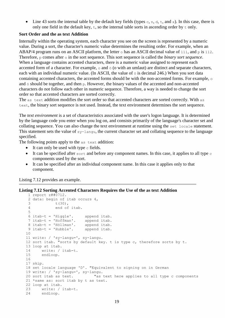
Listing 7.12 Sorting Accented Characters Requires the Use of the as text Addition 1 report z##0712.


3 t(30),

4 end of itab.

5

6 itab-t = 'Higgle'. append itab.

7 itab-t = 'Hoffman'. append itab.

8 itab-t = 'Höllman'. append itab.

9 itab-t = 'Hubble'. append itab.

10

11 write: / 'sy-langu=', sy-langu.

12 sort itab. "sorts by default key. t is type c, therefore sorts by t.

13 loop at itab.

14 write: / itab-t.

15 endloop.

16

17 skip.

18 set locale language 'D'. "Equivalent to signing on in German

19 write: / 'sy-langu=', sy-langu.

20 sort itab as text. "as text here applies to all type c components

21 *same as: sort itab by t as text.

22 loop at itab.

23 write: / itab-t.

24 endloop.

20

The code in Listing 7.12 produces this output: sy-langu= E

Higgle

Hoffman

Hubble

Höllman

sy-langu= D

Higgle

Hoffman

Höllman

Hubble

Lines 6 through 9 add four rows to the internal table. The one on line 8 contains an ö (o umlaut.)

Line 11 writes out the current logon language.

Line 12 sorts itab by the default key in binary sort sequence according to the current logon

language. The output shows that ö comes last in the sort sequence.

Set locale on line 18 changes the program's environment; it produces an effect similar to signing

on in German. Sy-langu is set to D, and the German character set and collating sequences are used

from that point forward in the program.

Line 20 uses sort with the as text addition after the internal table name. This causes as text to

apply to all type c components. In the output, o and ö appear together.

Sort sequences vary with platforms. When transporting from one operating system to another, the only

guaranteed sort sequences are A-Z, a-z, and 0-9, but not necessarily in that order.

TIP

After sorting, you can delete duplicates from an internal table using the delete

adjacent duplicates statement, described in the ABAP/4 keyword documentation.

Summary

An internal table is a collection of rows stored in RAM on the application server. It consists of a

header line and a body. The header line is optional. The header line is the implicit work area for the

internal table.

The existence of the occurs clause creates an internal table. It is used as a guideline for the system

to allocate memory. It does not limit the number of rows you can add to an internal table.

Use the loop at statement to retrieve multiple rows from an internal table. Each row is placed into

the header line or an explicit work area one at a time. Use from, to, and where to specify the rows

to be returned. Inside of the loop, sy-tabix contains the relative row number. After endloop, sy-

subrc will be zero if any rows were processed in the loop.

Inside of a loop, the flow of processing can be altered by an exit, continue, or check statement.

Exit terminates the loop and continues with the statement following the endloop. Continue

bypasses the remaining statements of the loop and immediately begins the next iteration. Check,

like continue, also begins a new iteration, but only does so when its logical expression is false.

Use the read table statement to locate a single row in the internal table. Using the index

addition, you can locate a single row by relative row number. This is the most efficient way to

locate a row. Using the with key addition, you can locate a row by specifying a value to be found.

comparing determines whether values in the work area differ from values in the found row.

transporting avoids unnecessary or undesired assignments from the found row to the work area.

The sort statement sorts an internal table by named components. If no components are named, the

table is sorted by its default key fields (types c, n, d, t, and x).

21

DO DON'T

DO use the binary search addition on the

read table statement. It will increase the

performance of the search tremendously.

DON'T use occurs 0 for internal tables

smaller than 8KB. This results in over-

allocation of memory and slower

performance.

DO use the index addition on the read table

statement whenever possible. It is the fastest

way to locate a single row.

22

Quiz Questions

1. Who sets a limit on the maximum amount of extended memory an internal table can allocate?

2. Why shouldn't you use occurs 0 if you expect to store less than 8KB in an internal table?

3. Can you use the read table statement to read database tables?

abap tutorial session 5 internal tablestutor.nmmu.ac.za/norma/wrer302/abap tutorial session 5.pdf1...

Documents