Ab initio STUDY OF THE EFFECT OF SOLUTEATOMS ON VACANCY DIFFUSION IN NI-BASEDSUPERALLOYS

by

KAMAL NAYAN GOSWAMI

A thesis submitted toThe University of Birminghamfor the degree ofDOCTOR OF PHILOSOPHY

School of Metallurgy and MaterialsCollege of Engineering and Physical SciencesThe University of BirminghamDecember 2016

University of Birmingham Research Archive

e-theses repository This unpublished thesis/dissertation is copyright of the author and/or third parties. The intellectual property rights of the author or third parties in respect of this work are as defined by The Copyright Designs and Patents Act 1988 or as modified by any successor legislation. Any use made of information contained in this thesis/dissertation must be in accordance with that legislation and must be properly acknowledged. Further distribution or reproduction in any format is prohibited without the permission of the copyright holder.

Dedicated to my late grandfather, who was the first teacher in my life

ACKNOWLEDGEMENTS

First and foremost, I would like to thank my PhD supervisor, Dr. Alessandro Mottura

for providing me the opportunity to work with him at the University of Birmingham and

for arranging for the School of Metallurgy and Materials scholarship that fully funded my

studies. His support and guidance was available throughout this work and his friendly

nature gave me the freedom to interact with him as much as I wanted to.

I would like to acknowledge the use of BlueBEAR High Performance Computing fa-

cility at the University of Birmingham as well as the MidPlus regional High Performance

Computing facility for the calculations presented in this thesis. I would also like to thank

the IT Services at the University of Birmingham for their help whenever required.

I express my gratitude to Dr. Hector Basoalto, who was my co-supervisor. I also

had the opportunity to work with him on the Ni-Al-Cr alloys as a side project. I thank

my colleagues- Lucia, Magnus, Gavin, Mohammad, Sebastian, Dimitra, Yogesh, Richard,

Chinnapat, Abed, Joshua and all the members of the CASIM research group for their

support and for providing a cheerful atmosphere in the IRC Netshape Lab.

I thank Anmol, Yasir, Sahara, Tania, Sabarinath, Kanika, Archontissa, Beate and all

the other friends for sharing their experiences and for their constant help during my PhD.

I had a great time with them over these years and they have given me loads of memories

to cherish for a long time.

Finally, I would like to thank my parents who were very supportive of my decision

to take up further studies. My brother, Ashish, motivated me through the tough times

and gave me the strength to keep going on. My family has been my source of inspiration

behind the completion of this thesis.

PUBLICATIONS

• K. N. Goswami and A. Mottura. Can slow-diffusing solute atoms reduce vacancy

diffusion in advanced high-temperature alloys?. Materials Science and Engineering:

A, 617:194-199, November 2014.

• K. N. Goswami and A. Mottura. A kinetic Monte Carlo study of vacancy diffusion

in non-dilute Ni-Re alloys (under preparation).

Abstract

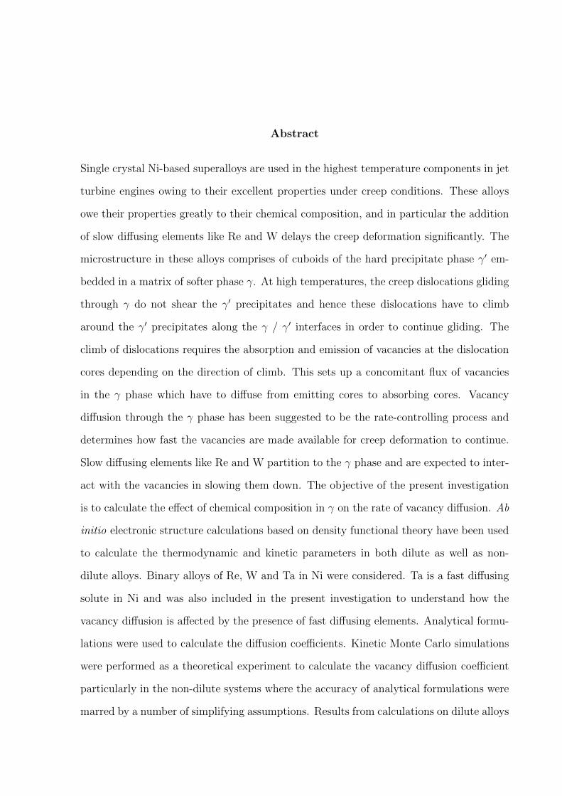
Single crystal Ni-based superalloys are used in the highest temperature components in jet

turbine engines owing to their excellent properties under creep conditions. These alloys

owe their properties greatly to their chemical composition, and in particular the addition

of slow diffusing elements like Re and W delays the creep deformation significantly. The

microstructure in these alloys comprises of cuboids of the hard precipitate phase γ′ em-

bedded in a matrix of softer phase γ. At high temperatures, the creep dislocations gliding

through γ do not shear the γ′ precipitates and hence these dislocations have to climb

around the γ′ precipitates along the γ / γ′ interfaces in order to continue gliding. The

climb of dislocations requires the absorption and emission of vacancies at the dislocation

cores depending on the direction of climb. This sets up a concomitant flux of vacancies

in the γ phase which have to diffuse from emitting cores to absorbing cores. Vacancy

diffusion through the γ phase has been suggested to be the rate-controlling process and

determines how fast the vacancies are made available for creep deformation to continue.

Slow diffusing elements like Re and W partition to the γ phase and are expected to inter-

act with the vacancies in slowing them down. The objective of the present investigation

is to calculate the effect of chemical composition in γ on the rate of vacancy diffusion. Ab

initio electronic structure calculations based on density functional theory have been used

to calculate the thermodynamic and kinetic parameters in both dilute as well as non-

dilute alloys. Binary alloys of Re, W and Ta in Ni were considered. Ta is a fast diffusing

solute in Ni and was also included in the present investigation to understand how the

vacancy diffusion is affected by the presence of fast diffusing elements. Analytical formu-

lations were used to calculate the diffusion coefficients. Kinetic Monte Carlo simulations

were performed as a theoretical experiment to calculate the vacancy diffusion coefficient

particularly in the non-dilute systems where the accuracy of analytical formulations were

marred by a number of simplifying assumptions. Results from calculations on dilute alloys

using analytical formulations based on Manning’s random alloy model suggested that the

role of both slow as well as fast diffusers on the vacancy diffusion coefficients was minimal.

However, results from kinetic Monte Carlo simulations on dilute as well as non-dilute al-

loys suggested appreciable modifications of the vacancy diffusion coefficients, suggesting

that the beneficial role of slow-diffusing atoms in Ni-based superalloys could be partly

explained by their effect on vacancy diffusion.

TABLE OF CONTENTS

1 Introduction 1

1.1 Physical metallurgy of Ni-based superalloys . . . . . . . . . . . . . . . . . 2

1.2 High temperature creep . . . . . . . . . . . . . . . . . . . . . . . . . . . . . 5

1.3 The Rhenium effect . . . . . . . . . . . . . . . . . . . . . . . . . . . . . . . 6

1.3.1 Solid solution strengthening . . . . . . . . . . . . . . . . . . . . . . 9

1.3.2 Stacking fault energy . . . . . . . . . . . . . . . . . . . . . . . . . . 10

1.3.3 Cluster formation and short range ordering . . . . . . . . . . . . . . 12

1.3.4 Enrichment at the γ/γ′ interface . . . . . . . . . . . . . . . . . . . 14

1.4 Dislocation mechanisms and the role of vacancy diffusion . . . . . . . . . . 17

1.5 Macroscopic diffusion theory . . . . . . . . . . . . . . . . . . . . . . . . . . 18

1.5.1 Fick’s laws of diffusion . . . . . . . . . . . . . . . . . . . . . . . . . 18

1.5.2 Kirkendall experiment and Darken’s equations . . . . . . . . . . . . 19

1.5.3 Tracer diffusion coefficients and thermodynamic factor . . . . . . . 21

1.6 Diffusion data in Ni-based superalloys . . . . . . . . . . . . . . . . . . . . . 22

2 Modelling diffusion 27

2.1 Modelling diffusion in dilute alloys . . . . . . . . . . . . . . . . . . . . . . 28

2.1.1 Calculation of self-diffusion and solute diffusion coefficients . . . . . 28

2.1.2 Calculation of vacancy diffusion coefficients . . . . . . . . . . . . . . 33

2.2 Kinetic Monte Carlo simulations . . . . . . . . . . . . . . . . . . . . . . . . 36

2.3 Modelling diffusion in non-dilute alloys . . . . . . . . . . . . . . . . . . . . 40

2.3.1 Cluster expansion method . . . . . . . . . . . . . . . . . . . . . . . 41

3 Computing Energies 45

3.1 Density functional theory . . . . . . . . . . . . . . . . . . . . . . . . . . . . 45

3.2 Nudged elastic band method . . . . . . . . . . . . . . . . . . . . . . . . . . 49

3.3 Settings for calculations . . . . . . . . . . . . . . . . . . . . . . . . . . . . 51

3.4 Convergence tests . . . . . . . . . . . . . . . . . . . . . . . . . . . . . . . . 52

4 Diffusion in dilute alloys 58

4.1 Results from analytical expressions . . . . . . . . . . . . . . . . . . . . . . 58

4.1.1 Lattice parameters and local relaxation around defects . . . . . . . 58

4.1.2 Vacancy formation energy . . . . . . . . . . . . . . . . . . . . . . . 60

4.1.3 Effective frequencies . . . . . . . . . . . . . . . . . . . . . . . . . . 61

4.1.4 Migration energy barriers . . . . . . . . . . . . . . . . . . . . . . . 62

4.1.5 Solute correlation factors . . . . . . . . . . . . . . . . . . . . . . . . 66

4.1.6 Ni-self diffusion coefficient and solute diffusion coefficients in Ni . . 70

4.1.7 Vacancy diffusion coefficients in Ni . . . . . . . . . . . . . . . . . . 74

4.2 Results from kinetic Monte Carlo Simulations in dilute alloys . . . . . . . . 76

4.2.1 Migration energy barriers for extended vacancy jumps . . . . . . . . 77

4.2.2 Ni-self diffusion coefficient and solute diffusion coefficients in Ni . . 80

4.2.3 Vacancy diffusion coefficients in Ni . . . . . . . . . . . . . . . . . . 83

4.2.4 Discussion . . . . . . . . . . . . . . . . . . . . . . . . . . . . . . . . 83

5 Binary cluster expansion in Nickel-Rhenium 86

5.1 Effective cluster interaction coefficients . . . . . . . . . . . . . . . . . . . . 89

5.2 Effective vacancy formation energy . . . . . . . . . . . . . . . . . . . . . . 96

5.3 Kinetically resolved activation energy barriers . . . . . . . . . . . . . . . . 98

6 Diffusion in non-dilute Nickel-Rhenium alloys 106

6.1 Error propagation in the calculated diffusivities . . . . . . . . . . . . . . . 107

6.2 Results in pure Ni . . . . . . . . . . . . . . . . . . . . . . . . . . . . . . . . 109

6.3 Results in non-dilute Ni-Re alloys . . . . . . . . . . . . . . . . . . . . . . . 113

6.3.1 Monte Carlo simulations . . . . . . . . . . . . . . . . . . . . . . . . 114

6.3.2 Vacancy diffusion coefficients . . . . . . . . . . . . . . . . . . . . . 117

6.3.3 Ni and Re diffusion coefficients . . . . . . . . . . . . . . . . . . . . 121

6.3.4 Correlation factors . . . . . . . . . . . . . . . . . . . . . . . . . . . 127

6.3.5 Variation of D0 and Q as a function of composition . . . . . . . . . 128

6.3.6 Comparison with the kMC results on dilute alloys . . . . . . . . . . 132

6.3.7 Discussion . . . . . . . . . . . . . . . . . . . . . . . . . . . . . . . . 133

7 Conclusions and Scope for Future Work 137

List of References 140

LIST OF FIGURES

1.1 A schematic of the longitudinal section of a jet engine showing the mate-

rials used. Ni-based superalloys (in yellow) are used in the combuster and

turbine sections . . . . . . . . . . . . . . . . . . . . . . . . . . . . . . . . . 2

1.2 Ni representing the γ phase and Ni3Al the ordered γ′ phase. In a superalloy,

various alloying additions are made which substitute for Ni or Al in one or

both the phases . . . . . . . . . . . . . . . . . . . . . . . . . . . . . . . . 2

1.3 The γ-γ′ microstructure of a commercial superalloy CMSX-4 . . . . . . . . 3

1.4 The turbine blades in equiaxed, columnar and single crystal forms . . . . . 4

1.5 Trends in the Ni-based superalloy chemistry over the years . . . . . . . . . 4

1.6 Applied stress and temperature conditions for the different creep regimes

to operate . . . . . . . . . . . . . . . . . . . . . . . . . . . . . . . . . . . . 6

1.7 Constant load creep data for CMSX-4 in different regimes . . . . . . . . . 7

1.8 Effect of Re addition on a model alloy 444 (Temperature =1172 K, applied

stress =380 MPa) . . . . . . . . . . . . . . . . . . . . . . . . . . . . . . . . 8

1.9 Solid solution hardening potency for the different solutes in binary Ni alloys 10

1.10 Two Shockley partials and a stacking fault on a {111} plane in the γ phase 11

1.11 Calculated binding energies for Re-Re, W-W and Ta-Ta pairs . . . . . . . 13

1.12 Combined glide-plus-climb mechanism in the tertiary regime . . . . . . . . 16

1.13 A schematic of the Kirkendall’s diffusion experiment on α-brass (source -

Wikipedia) . . . . . . . . . . . . . . . . . . . . . . . . . . . . . . . . . . . . 19

1.14 Arrhenius plot of self diffusion coefficient of Ni in single crystals from low

to high temperatures . . . . . . . . . . . . . . . . . . . . . . . . . . . . . . 23

1.15 Interdiffusion coefficients in the γ phases of Ni-Ta, Ni-W and Ni-Re systems 23

1.16 Results from ab initio calculations of Janotti et al . . . . . . . . . . . . . . 25

1.17 Vacancy diffusion coefficients for different concentrations of Re and Ta in

Ni as calculated by Schuwalow et al . . . . . . . . . . . . . . . . . . . . . . 26

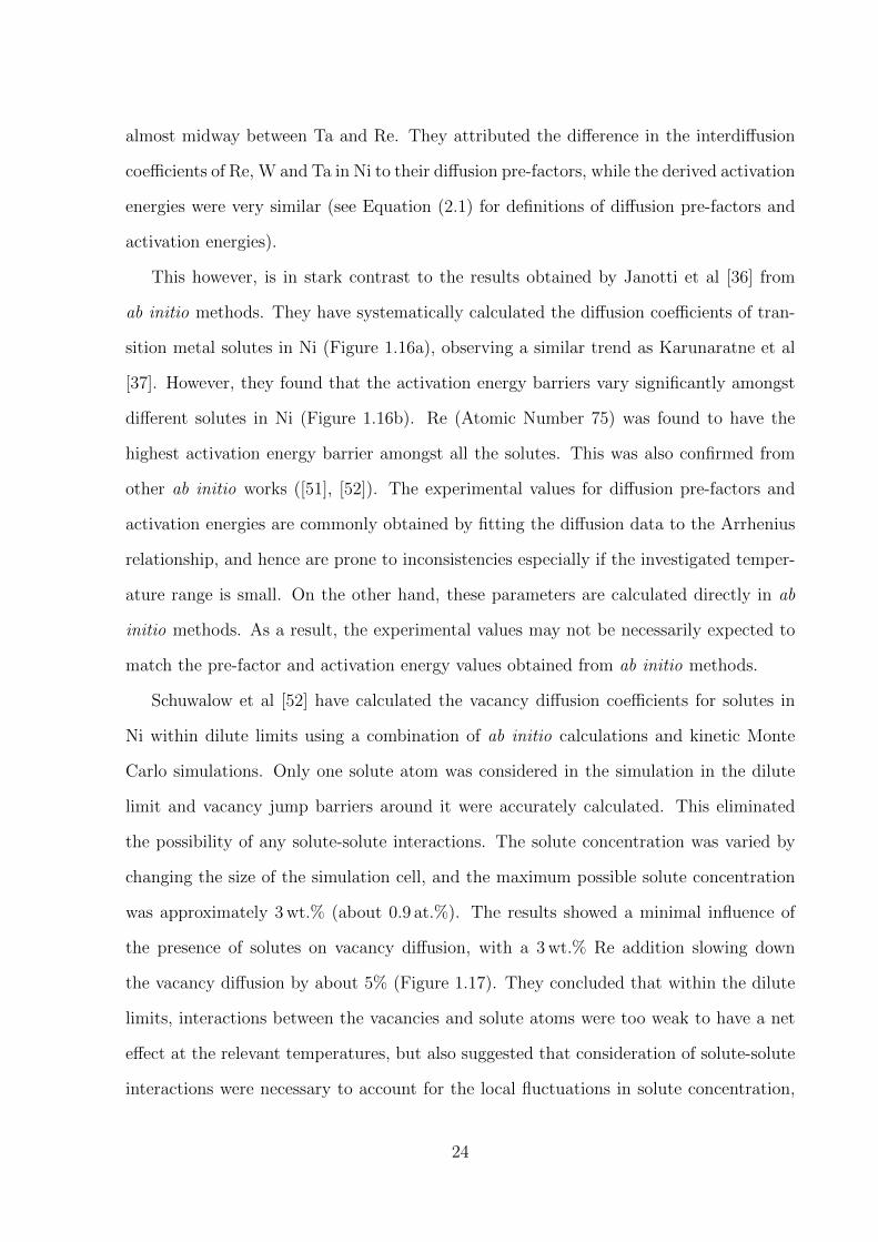
2.1 Vacancy assisted diffusion in a dilute fcc alloy . . . . . . . . . . . . . . . . 29

2.2 The atom-vacancy exchange showing an migration energy barrier . . . . . 31

2.3 Various diffusion jumps in a dilute fcc alloy causing a vacancy-solute ex-

change, rotation and dissociation/association . . . . . . . . . . . . . . . . . 32

2.4 Contour plot showing an atom vibrating at its equilibrium position, and a

rare diffusive jump by surmounting of the energy barrier . . . . . . . . . . 38

2.5 A 2D lattice showing some possible clusters . . . . . . . . . . . . . . . . . 41

2.6 The physical representation of the effective vacancy formation energy . . . 42

2.7 A schematic diagram illustrating the meaning of the kinetically resolved

activation energy barriers . . . . . . . . . . . . . . . . . . . . . . . . . . . . 44

3.1 The initial and final configurations in a 2-D energy landscape using NEB

method with 16 images. The initial linearly interpolated configuration

finally converges to the MEP . . . . . . . . . . . . . . . . . . . . . . . . . . 50

3.2 The plain elastic band results for a case with a curved path near the saddle

point (a) k=1.0, and (b) k=0.1. The result for a NEB is shown by a solid

line which goes through the saddle point . . . . . . . . . . . . . . . . . . . 51

3.3 The convergence of energy per atom in Ni at different values of energy cutoffs 53

3.4 The convergence of energy per atom in Ni with different k-point densities . 54

3.5 Results for convergence tests in Re . . . . . . . . . . . . . . . . . . . . . . 55

3.6 Results for convergence tests in W . . . . . . . . . . . . . . . . . . . . . . . 56

3.7 Results for convergence tests in Ta . . . . . . . . . . . . . . . . . . . . . . 57

4.1 The binding energies of solute-� pairs at various distances in the Ni lattice 60

4.2 The minimum energy path connecting the initial and final end states for

various solute-� jumps . . . . . . . . . . . . . . . . . . . . . . . . . . . . . 65

4.3 An fcc cell showing a solute atom (black), a vacancy (empty square), the Ni

atoms (green) and their nearest neighbour relationship to the solute atom

and the various vacancy jumps corresponding to the calculated migration

barriers. There are more than one symmetrically equivalent atoms, but only

one case of solute-� pair rotation and solute-� pair dissociation/association

has been shown for clarity. . . . . . . . . . . . . . . . . . . . . . . . . . . 67

4.4 The solute correlation factors fi calculated in the temperature range of

1173 K to 1573 K. . . . . . . . . . . . . . . . . . . . . . . . . . . . . . . . 68

4.5 The self-diffusion coefficient of Ni calculated from first principles compared

to experimental values . . . . . . . . . . . . . . . . . . . . . . . . . . . . . 71

4.6 (a)The solute diffusion coefficients in Ni as a function of temperature. Ni-

self diffusion coefficient has been included as well for comparison. (b)-(d)

Comparison of the solute diffusion coefficients to previous works in the

literature . . . . . . . . . . . . . . . . . . . . . . . . . . . . . . . . . . . . . 72

4.7 Vacancy correlation factors in Ni at 1373 K . . . . . . . . . . . . . . . . . 75

4.8 Vacancy diffusion coefficients in Ni as a function of solute concentration at

1373 K . . . . . . . . . . . . . . . . . . . . . . . . . . . . . . . . . . . . . . 76

4.9 Possible jumps within 4th nearest neighbour distance of the solute atom

(Image recreated from Schuwalow et al ). The green atoms are Ni atoms,

the black atom is the solute atom and the square box represents the va-

cancy. The numbers on the atoms/vacancy represent their nearest neigh-

bour distance with respect to the solute atom. Symmetrically equivalent

jumps have not been shown. . . . . . . . . . . . . . . . . . . . . . . . . . . 78

4.10 The self-diffusion coefficient in Ni and solute diffusion coefficients in Ni as

a function of temperature. The symbols represent the results from kMC

simulations, while the lines represent the results calculated from Lidiard’s

model . . . . . . . . . . . . . . . . . . . . . . . . . . . . . . . . . . . . . . 82

4.11 Vacancy diffusion coefficients in Ni as a function of solute concentration at

1373 K as calculated from the kMC simulations in dilute alloys . . . . . . . 84

5.1 The formation energy calculated for the 144 Ni-Re configurations. 101 of

these configurations were used in the cluster expansion to get the ECIs. . 89

5.2 ECI/multiplicity for pair and triplet clusters . . . . . . . . . . . . . . . . . 90

5.3 The pair and triplet clusters used in the ECI fitting . . . . . . . . . . . . . 92

5.4 Comparison of the Re-Re binding energies from first principles, predictions

from cluster expansion and non-spin polarized results from Mottura et al . 95

5.5 The clusters used for expansion of the effective vacancy formation energy

(adopted from Van der Ven et al . . . . . . . . . . . . . . . . . . . . . . . . 96

5.6 The calculated local effective cluster expansion coefficients for cluster num-

bers 1 - 6. The corresponding clusters have been shown in Figure 5.5. Red,

green and blue symbols represent point, pair and triplet clusters around a

vacancy . . . . . . . . . . . . . . . . . . . . . . . . . . . . . . . . . . . . . 97

5.7 Comparison of the Re-� binding energies from first principles with predic-

tions from local cluster expansion. The scale is kept similar to Figure 5.4. . 99

5.8 Configurations used for Re jumps . . . . . . . . . . . . . . . . . . . . . . . 100

5.9 Configurations used for Ni jumps when the Re atoms are paired . . . . . . 101

5.10 Configurations used for Ni jumps when the Re atoms are unpaired . . . . . 102

5.11 The fcc {111} plane showing an atom in black next to a vacancy surrounded

by other atoms in the 1st nearest neighbour shell. The colour of these atoms

represent their relationship to the black atom and the vacancy. Atoms out

of the plane have been shown smaller in size. . . . . . . . . . . . . . . . . 105

6.1 The self-diffusion coefficient in Ni and Re diffusion coefficient in Ni as a

function of temperature. The open symbols represent the results from the

kMC simulations using our code for non-dilute alloys, the filled symbols

represent the results from the kMC simulations using the code provided by

Dr. Sergej Schuwalow for dilute alloys and the lines represent the results

calculated from Lidiard’s model . . . . . . . . . . . . . . . . . . . . . . . . 113

6.2 Changes in the configuration of Re atoms for a binary Ni alloy containing

5 at.% Re during the course of the Monte Carlo simulation at 1373 K. The

size of the fcc simulation cell is 15 × 15 × 15 and the Ni atoms have been

deleted for clarity. a, b and c represent the three orthogonal directions. . . 116

6.3 Energy of a simulation cell of 5 at.% Re at 1373 K during the course of a

Monte Carlo simulation . . . . . . . . . . . . . . . . . . . . . . . . . . . . . 117

6.4 Energy of a simulation cell of 5 at.% Re at 1373 K as a function of kMC

simulation time (the energy scale has been kept the same as in Figure 6.3

for comparison) . . . . . . . . . . . . . . . . . . . . . . . . . . . . . . . . . 118

6.5 The running average of the vacancy diffusion coefficient for an alloy with

5 at.% Re at 1373 K as a function of simulation time . . . . . . . . . . . . 119

6.6 Calculated Dv in the non-dilute regime in Ni-Re at 1373 K . . . . . . . . . 119

6.7 Calculated Dv in the non-dilute regime in Ni-Re at different temperatures . 120

6.8 Calculated DNi in the non-dilute regime in Ni-Re at 1373 K . . . . . . . . 122

6.9 Calculated DRe in the non-dilute regime in Ni-Re at 1373 K . . . . . . . . 123

6.10 Calculated DNi in the non-dilute regime in Ni-Re at different temperatures 125

6.11 Calculated DRe in the non-dilute regime in Ni-Re at different temperatures 126

6.12 Calculated correlation factors in the non-dilute regime in Ni-Re at 1373 K 128

6.13 Calculated diffusion pre-factors as a function of Re composition in Ni . . . 130

6.14 Calculated activation energies as a function of Re composition in Ni . . . . 131

6.15 Comparison of the calculated Dv in the dilute and the non-dilute regime

in Ni-Re at 1373 K . . . . . . . . . . . . . . . . . . . . . . . . . . . . . . . 132

LIST OF TABLES

4.1 The calculated change in the macroscopic lattice parameter (∆a) and the

percentage local relaxation for a vacancy and for Re, W and Ta in Ni . . . 59

4.2 The calculated effective frequencies for Ni, Re, W and Ta . . . . . . . . . . 62

4.3 The calculated terms for self-diffusion and solute diffusion in Ni . . . . . . 69

4.4 The migration barriers for solute-� exchange and solute-� extended rota-

tion, dissociation and association used in the kinetic Monte Carlo simula-

tions for dilute alloys . . . . . . . . . . . . . . . . . . . . . . . . . . . . . . 79

4.5 The Di0 and Qi terms extracted from the kMC data for self-diffusion and

solute diffusion in Ni compared to the previously calculated results from

Lidiard’s model (LM) in the present work . . . . . . . . . . . . . . . . . . 81

5.1 The calculated effective cluster interaction coefficients (ECIs) . . . . . . . . 91

5.2 The first principles energy and energy predicted from cluster expansion of

Ni-Re by the CASM code for pure Ni and pure Re . . . . . . . . . . . . . . 94

5.3 Comparison of the binding energies for different Re clusters from first prin-

ciples, predictions from cluster expansion and non-spin polarized results

from Mottura et al . . . . . . . . . . . . . . . . . . . . . . . . . . . . . . . 95

5.4 The calculated local effective cluster expansion coefficients (LECIs) . . . . 98

5.5 KRAs calculated for the various Re jumps . . . . . . . . . . . . . . . . . . 100

5.6 KRAs calculated for the various Ni jumps . . . . . . . . . . . . . . . . . . 103

6.1 The calculated total energies and vacancy formation energies in pure Ni,

∆Ef,Ni for different simulation cell sizes (see Equation (2.9)) . . . . . . . . 110

6.2 The calculated Dv in pure Ni for various kMC segment lengths (total num-

ber of jumps is 1 billion in each case) compared to the Dv calculated from

analytical formulation with ∆Em,i of 1.08 eV (see Equation (2.6)) . . . . . 112

6.3 The vacancy diffusion coefficient in pure Ni and the calculated slope for Dv

as a function of temperature . . . . . . . . . . . . . . . . . . . . . . . . . . 121

6.4 The self-diffusion coefficient in pure Ni and the calculated solvent enhance-

ment factors for DNi as a function of temperature . . . . . . . . . . . . . . 123

6.5 The Re diffusion coefficient in the dilute case and the calculated solute

enhancement factors for DRe as a function of temperature . . . . . . . . . . 124

6.6 Re composition in γ phase (xRe) and time to rupture (tr) for some super-

alloys studied by Blavette et al at 1123 K and 500 MPa . . . . . . . . . . . 136

6.7 Dv corresponding to Re composition in binary Ni-Re alloys at 1173 K

calculated in the present work . . . . . . . . . . . . . . . . . . . . . . . . . 136

CHAPTER 1

INTRODUCTION

Ni-based superalloys represent a class of materials designed to withstand extreme condi-

tions [1]. Their excellent performance under high temperature creep conditions, amongst

others, make them suitable for applications such as turbine blades in gas turbine engines

used for jet propulsion in civil and military aircrafts (see Figure 1.1). From thermody-

namic considerations, high engine efficiencies are achieved at high operating temperatures

and over the past few decades, the improvements in superalloy technology have raised the

temperature capability of the gas turbine engines beyond 1273 K [1]. This has mostly

been achieved by altering the chemical composition of these superalloys considerably. The

addition of Re, a rare and expensive metal, in particular was seen to have a strong creep

strengthening effect. But even as the improvement in strength is clearly seen, an un-

derstanding of the fundamental mechanism leading to the observed strengthening is still

lacking [2]. High temperature creep is dependent on the rate of vacancy diffusion and an

accepted argument within the superalloys community is that slow diffusing atoms, like

Re, slow down the vacancy diffusion, leading to the lowering of creep deformation rate

[2]. Other important elements like Ta, W and Mo are also potent strengtheners, albeit to

a lesser degree. The present work aims at investigating the effect of various alloying ad-

ditions on the vacancy diffusion in Ni based superalloys from a variety of computational

techniques in an attempt to explain the observed strengthening as well as to generate

meaningful diffusion data for future alloy design programmes.

1

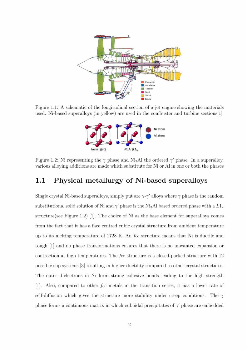
Figure 1.1: A schematic of the longitudinal section of a jet engine showing the materialsused. Ni-based superalloys (in yellow) are used in the combuster and turbine sections[1]

Figure 1.2: Ni representing the γ phase and Ni3Al the ordered γ′ phase. In a superalloy,various alloying additions are made which substitute for Ni or Al in one or both the phases

1.1 Physical metallurgy of Ni-based superalloys

Single crystal Ni-based superalloys, simply put are γ-γ′ alloys where γ phase is the random

substitutional solid solution of Ni and γ′ phase is the Ni3Al based ordered phase with a L12

structure(see Figure 1.2) [1]. The choice of Ni as the base element for superalloys comes

from the fact that it has a face centred cubic crystal structure from ambient temperature

up to its melting temperature of 1728 K. An fcc structure means that Ni is ductile and

tough [1] and no phase transformations ensures that there is no unwanted expansion or

contraction at high temperatures. The fcc structure is a closed-packed structure with 12

possible slip systems [3] resulting in higher ductility compared to other crystal structures.

The outer d-electrons in Ni form strong cohesive bonds leading to the high strength

[1]. Also, compared to other fcc metals in the transition series, it has a lower rate of

self-diffusion which gives the structure more stability under creep conditions. The γ

phase forms a continuous matrix in which cuboidal precipitates of γ′ phase are embedded

2

Figure 1.3: The γ-γ′ microstructure of a commercial superalloy CMSX-4 [1]

in a coherent manner with its <001> crystallographic direction aligned to the <001>

crystallographic direction of the γ phase. The γ′ phase gives order strengthening and

exhibits anomalous yielding phenomena, a characteristic unique to some L12 phases where

the strength of the γ′ phase increases with temperature [4]. For this reason, their volume

fraction is kept as high as 70 %. Figure 1.3 shows a typical microstructure for a commercial

Ni-based superalloy CMSX-4. One can clearly see the high volume fraction of the γ′ phase

embedded in thin γ matrix. There are other phases known as Topologically Closed Packed

(TCP) phases [5] which sometimes form during processing or service conditions, however

they are detrimental to the creep performance and are hence undesirable.

From a historical point of view, the superalloys have been in use since the 1940s.

Advancements in the casting technologies led to a shift from wrought to cast alloys with

equiaxed structure, and then from equiaxed structure to columnar structure using direc-

tional solidification methods (see Figure 1.4) [1]. Modern day turbine blades are made

of single crystal superalloys using the investment casting methods [6]. These alloys show

drastic improvements in creep performance when compared to the previous versions. As

grain boundaries are completely removed, grain boundary sliding/migration which are

3

Figure 1.4: The turbine blades in equiaxed, columnar and single crystal forms [1].

common at high temperatures are taken out of the equation [1]. Also, elements like B

and C previously added to the polycrystalline Ni-based superalloys, which promoted the

formation of eutectic mixtures during casting, are no longer needed. Absence of grain

boundaries also reduces the occurrence of incipient melting during further heat treat-

ments. The as-cast dendritic structure is homogenised by a solutioning treatment to

remove the micro-segregation in the composition and to dissolve eutectic mixtures rich in

γ′. Further ageing treatment leads to the formation of γ′ precipitates with optimum size

and uniform distribution [1].

Figure 1.5: Trends in the Ni-based superalloy chemistry over the years [1].

Superalloys are highly alloyed systems with over 10 alloying additions (see Figure 1.5).

Each added element has a specific role and a preference for a particular phase. The most

common elements include Al, Ta, Ti, W, Re, Mo, Cr, Co and Ru. Grain boundary

strengthening elements like B and C which were added earlier are no longer needed since

modern blades used in the hottest parts of jet engines are now single-crystal blades. Al and

4

Ta are strong γ′ formers and are present in appreciable amounts in modern superalloys.

W, which otherwise partitions to the γ′ phase is rejected towards γ in the presence of

Ta [7] where it acts as a solid solution strengthener. Re, the main subject of the current

study, on the other hand strongly partitions to the γ phase and has a dramatic effect

on improving the creep lives of superalloys [8]. Infact, second and third generation of

superalloys are marked by the addition of 3 wt. % and 6 wt. % of Re respectively

[1]. Fourth generation superalloys are marked by the addition of Ru which reduces the

propensity of the formation of TCP phases on the addition of Re [9].

1.2 High temperature creep

Creep is a manifestation of inelastic behaviour which becomes significant in metals only

at high temperatures, where the strain in the material increases with time under constant

stress. This occurs even at stresses substantially lower than the yield strength of the ma-

terial. Ni-based superalloys are used in high temperature applications where deformation

due to creep becomes significant. As an example, in CMSX-4, which is a second genera-

tion superalloy, the yield strength at 1223 K is about 600 MPa, however even a stress of

200 MPa can cause a creep strain of 5 % after 1800 h [1]. Consequently, with time, strain

will be accumulated and excessive creep deformation will cause failure of the component.

The jet engine components such as the turbine blades are machined to fit tight tolerances

and hence creep strains greater than a few percent render them unfit for service[1].

In the case of Ni-based superalloys, a number of regimes for the different mechanisms

of creep deformation have been identified based on the applied stress and temperature

as shown in Figure 1.6 [1]. Figure 1.7 shows the creep curves in different regimes for a

second-generation superalloy CMSX-4. At low temperatures (<1023 K), the superalloys

undergo primary creep deformation with a decrease in strain rate with strain. Shear-

ing of the γ′ precipitates is possible at sufficiently high stresses (>500 MPa) by complex

dislocation reactions. Creep at very high temperatures (>1323 K) is characterised by di-

5

Figure 1.6: Applied stress and temperature conditions for the different creep regimes tooperate [1].

rectional coarsening of the γ′ precipitates to form rafts and by the formation of equilibrium

dislocation networks at the γ/γ′ interfaces [10].

However, across wide ranges of temperatures and applied stresses, in the intermediate

tertiary regime, creep dislocations do not penetrate the γ′ precipitates [1]. The slip is of

the a/2<110>{111} type and is limited to the γ channels. The dislocations dissociate into

two Shockley partials of the a/6<112> type separated by an intrinsic stacking fault. No

shearing of the γ′ precipitates occur, and hence, substantial cross-slip or climb is required

for the dislocations to avoid the precipitates. The creep therefore occurs by a glide-plus-

climb mechanism. The glide step produces almost all of the strain, but the climb controls

the velocity. And since dislocation climb relies on diffusional processes, it can be assumed

that the rate controlling step is diffusion [2].

1.3 The Rhenium effect

The first generation of single crystal Re-free superalloys were followed by the second

generation superalloys in the 1990s and third generation superalloys in the 2000s marked

by the addition of 3 wt.% and 6 wt.% Re respectively. The pioneering studies on the

Re addition to single crystal Ni-based superalloys was conducted by Giamei et al [8, 11].

6

Figure 1.7: Constant load creep data for CMSX-4 in different regimes [1].

7

Figure 1.8: Effect of Re addition on a model alloy 444 (Temperature =1172 K, appliedstress =380 MPa)[11].

In this study, Re was added to a modified MAR-M200 alloy to replace W, keeping the

W+Re wt.% constant. Four alloys with 0, 2 , 4 and 6 wt.% Re were tested in creep at

1172 K and 380 MPa. Figure 1.8 shows the tertiary creep curves from the study of Giamei

et al [11] clearly demonstrating how Re addition helps delay the accumulation of creep

strain. Since then several other investigtions have been carried out, which confirmed the

beneficial role of Re addition under tertiary creep [12, 13, 14, 15]. However, Re is one of

the most expensive transition metals, so much so that it could be responsible for up to

half the cost of the raw material needed to make the turbine blades [2] .The high price and

limited availability of Re makes it important to understand the underlying mechanisms

for the observed creep strengthening, such that in the future, the amount of Re added

can be reduced for cost related benefits.

Re almost entirely partitions to the γ phase, reduces the γ′ coarsening rate and also

increases the γ/γ′ misfit . However, these properties do not explain the beneficial role

of Re as seen in the tertiary creep regime in Ni-based superalloys. Several investigations

8

have been carried out to elucidate the role of Re in creep strengthening.

1.3.1 Solid solution strengthening

Addition of solute atoms to a solvent lattice forms a solid solution which is invariably

stronger than the solvent [3]. The solute additions increase the yield stress and the level

of the stress-strain curve as a whole [16]. These solute atoms, thus, offer resistance to

dislocation motion, which leads to the observed strengthening. Traditionally, the solid

solution strengthening is thought to be related to the elastic interaction between the solute

atoms and the dislocations owing to the size misfit between the solute and the solvent

atoms. The distortions produced by the solute atoms in the solvent lattice interact with

the elastic stress fields produced by the core of the dislocations, and hence the solid

solution strengthening should be directly proportional to the size misfit of the solute

atom. However, this is not the case as other factors also play an important role. Solid

solution strengthening also encompasses other effects such as modulus misfit, valence

effects, effects on stacking fault energy (see Section (1.3.2) ). Also, clustering and short

range ordering can play a role, more on which has been discussed in Section (1.3.3). Since

creep deformation is mostly limited to the γ phase at high temperatures, it is reasonable

to assume that Re plays a part in hindering dislocation glide in the γ phase.

Gan et al [17] used variety of instrumented indentation techniques to quantify the

degree of solid solution strengthening for many transition metals in binary Ni alloys.

It was ensured that all the binary alloys were single phase γ alloys and were properly

homogenized to do away with any role of clustering or ordering. It was shown that the

solutes which had a larger atomic radius also showed a higher compressibility in the Ni

lattice and hence the effect of atomic size misfit was minimum. The alloy hardness was

found to vary with the solute species with Nb, Ta, Rh and Ir showing maximum potency

for solid solution hardening, while Re only had a minimal effect (see Figure 1.9). It was

argued that the potency of solute atoms in solid solution strengthening should be governed

by their effect on the stacking fault energies in Ni.

9

Figure 1.9: Solid solution hardening potency for the different solutes in binary Nialloys[17].

1.3.2 Stacking fault energy

The slip system in fcc crystals is a/2<110>{111} which means the deformation in these

crystals should take place by the gliding of dislocations causing a slip along the 1/2<110>

direction on the close-packed {111} planes. However, it is energetically favourable for

these dislocations to split into two partial dislocations of the a/6<112> type. These

dislocations are known as Shockley partials. One can clearly see that the reaction is

energetically favourable by applying the Frank’s rule, which states that the energy of a

dislocation is proportional to the square of its Burgers vector [18]:

a

2〈110〉{111} → a

6〈211〉{111}+

a

6〈121〉{111} (1.1)

The passage of a perfect dislocation does not create a planar defect. However, the

passage of the first Shockley partial dislocation creates an intrinsic stacking fault (ISF)

by locally changing the atomic coordination. In fcc crystals, the ABCABCABCABC

packing sequence is changed to ABCACABCABC, thus creating two neighbouring planes

with the hcp coordination locally [18]. This intrinsic stacking fault is removed on the

passage of the second Shockley partial dislocation [18]. Thus, in principle, we have two

10

Figure 1.10: Two Shockley partials and a stacking fault on a {111} plane in the γ phase[1].

partial dislocations and a stacking fault in between (see Figure 1.10). When encountering

a barrier, these partial dislocations must recombine for either cross-slip or climb depending

on their character, i.e. edge or screw. The separation between the two partial dislocations

depends on their elastic repulsion and also on the stacking fault energy (SFE) [18]. The

lower the SFE, the larger is the separation between the two partial dislocations, and

it is comparatively difficult for them to come together and recombine. Thus, another

hypothesis for the observed creep strengthening by Re could be connected to the fact

that it may play a significant role on the reduction in SFE in Ni-based superalloys [19].

Ni has one of the highest SFE of the various fcc metals. This is of the order of 120 - 130

mJ/ m2 [20], and almost all alloying additions lower the SFE values in Ni. Yu et al [21]

and Shang et al [20] studied the effect of alloying additions on the SFE in dilute binary

alloys of Ni using density functional theory calculations. A reduction of about 25 mJ/m2

was calculated for Re at a temperature of 0 K. This reduction increases further at 300 K.

However, the reduction was similar in magnitude to other alloying elements like W and

Mo. Thus, Re does not overshadow the others in terms of reduction in SFE. Pettinari et

al [22] and Diologent et al [23] have also examined the role of Re on SFE in the γ phase of

commercial Ni-based superalloys through experiments. Different alloys with and without

Re were studied with a wide range of variation in composition. However, both studies

confirmed that there was hardly any difference between the SFE of Ni-based alloys with

and without Re, and the values always lie between 20 - 32 mJ/m2 Hence, the hypothesis

11

that Re plays a significant role in the reduction of SFE in Ni-based superalloys has to be

excluded.

1.3.3 Cluster formation and short range ordering

Blavette et al [12] had suggested from 1-dimensional atom probe tomography studies that

Re forms clusters in Ni, a finding that was later supported by Wanderka et al [24]. Clusters

of solute atoms can act as better hindrance to dislocation glide than individual solute

atoms and hence they argued that the observed creep strengthening on Re addition is due

to the formation of Re clusters in Ni. Indeed, the Ni-Re system shows a miscibility gap

[25] and hence one could expect Re to show clustering especially at lower temperatures,

however, since the operating temperatures of Ni-based superalloys is high, the entropy

effects are likely to overcome these clustering tendencies. In their studies, Blavette et

al [12] and Wanderka et al [24] found that the number of Re atoms in different atomic

layers showed a deviation from that expected from a random distribution of Re atoms.

Some atomic layers had fewer than random number of Re atoms, while other layers had

more than a random number of Re atoms. However, the conclusions from these 1-D

APT studies were based on datasets which consisted of a few thousand atoms, and hence

the statistical viabilty of these studies can be questioned. Moreover, these deviations

from random distribution do not clarify if there is a tendency for clustering or short range

ordering (SRO). Later 3-D APT studies were conducted by Mottura et al [26, 27] to study

the Re-clustering in Ni-based superalloys as well as in binary Ni-Re alloys. 3-D APT had

a clear advantage over 1-D APT in terms of statistical accuracy given that the dataset

collected consisted of hundreds of millions of atoms. Their results clearly showed that Re

is distributed randomly in Ni and that the presence of some clusters is indispensible due

to the statistical fluctuations. However, one must point out that the use of APT to study

clustering can be problematic since there are systematic errors in the measured atomic

positions. Other techniques like extended X-Ray absorption fine spectroscopy (EXAFS)

which can determine the local atomic environment around an atom was also conducted

12

Figure 1.11: Calculated binding energies for Re-Re, W-W and Ta-Ta pairs [29].

by Mottura et al [28] to study Re clusters in Ni. Again, results from these studies showed

that Re is coordinated by 12 Ni atoms, and no evidence was found for Re clustering in

Ni.

To complement these experimental studies, Mottura et al [29] also performed theoret-

ical calculations based on density functional theory. Binding energies were calculated for

Re-Re nearest neighbour pairs in Ni and these results are shown in Figure 1.11 together

with the results for Ta and W. From definition, a negative binding energy means that the

pair is energetically unfavourable. A negative binding energy was calculated for the Re-Re

first nearest neighbour pairs while on further separation of Re atoms, the magnitude of

the binding energy dropped significantly. Similar results were found for Ta and W. Also,

binding energy calculations on small Re clusters up to 4 atoms in size also showed that

they were energetically unfavourable. It must, however, be pointed that the calculations

performed by Mottura et al [29] did not include magnetism and it is a matter of debate

whether results from non-magnetic calculations at 0 K are representative of Ni alloys at

high temperature as Ni loses its ferromagnetic property above its Curie temperature of

630 K [30]. According to He et al [31], the local magnetic moments in Ni fluctuate at fi-

nite temperatures leading to a nonzero local magnetic moment. A complete consideration

of the Gibbs free energy at high temperature should thus include the thermal magnetic

13

excitations, which is a formidable task at the present time [31]. Indeed, He et al [31] have

calculated enthalpies of formation in various Ni-Re alloys and found that magnetism plays

an important role. The nonmagnetic and ferromagnetic formation enthalpies of random

alloys in the Ni rich part of the Ni-Re system showed a drastic change from ordering to

phase separation [31]. Other theoretical studies [32] predicted the presence of an ordered

intermetallic Ni4Re with the D1a structure from ferromagnetic calculations in the Ni-Re

system at lower temperatures. This intermetallic phase is expected to dissolve at higher

temperatures due to entropy effects, but the authors argued that some remnant short

range ordering is expected. However, given the slow diffusion rate of Re in Ni, the forma-

tion of this ordered intermetallic phase at lower temperatures and the associated SRO is

questionable, and needs to be validated by experiments.

1.3.4 Enrichment at the γ/γ′ interface

Re enrichment in the γ phase close to the γ/γ′ interfaces was observed in several Ni-based

superalloys [33, 34] from atom probe studies. Given that the dislocations have to climb

at the γ/γ′ interfaces for creep deformation to proceed, such enrichments could pin the

dislocations, making it difficult for them to climb. This enrichment appeared to be in

the form of a ’bow wave’ of Re in the γ phase ahead of the γ′ interface [33, 34] and it

was more pronounced than some of the other elements. Ge et al [35] on the other hand

found no evidence of Re enrichments in the γ phase in the uncrept samples, but found

regions enriched in Re in the γ phase close to the interface in the crept samples. They

also argued that aggregation of Re near the dislocation cores, would mean that vacancies

would have to exchange positions with a Re atom for climb, and given the high energy

barrier for this [36], it would make climb more difficult.

Given these observations, it was important to understand if the observed enrichment

was due to the rejection of Re during coarsening of the γ′ precipitates at the service

temperature or was it because of the γ′ phase growth on cooling. In either case, the

movement of the γ/γ′ interface could be achieved by the diffusion of γ′ forming elements

14

like Al and Ta towards the γ′ phase, with a concomitant rejection of γ phase formers

like Re. Phase field simulations were done to understand this phenomena by Mottura

et al [27] by predicting the γ/γ′ interface growth on cooling from high temperatures and

the simulations accurately predicted the composition profiles close to the γ/γ′ interfaces

when compared to their own atom probe data. It was shown that the movement of the

γ/γ′ interface was strongly dependent on the cooling rate and the interface movement

was small on fast cooling, which can possibly explain why no Re enrichment was found

in the case of Ge et al [35] for uncrept samples. Thus, it was clear that the growth

of the γ/γ′ interface is diffusion-limited, as the diffusion of solute elements is not fast

enough to reach equilibrium. Given the replication of the enrichment/depletion of the

solute elements near the interface by these cooling simulations when compared to the

experiments, it was concluded that the observed Re enrichment was due to the rejection

of Re from the growing γ′ precipitates on cooling from high temperatures and that such

enrichments were not expected at the service temperatures [27]. It was also observed that

in cases where secondary γ′ precipitates formed inside the γ matrix, the extent of the γ/γ′

interface migration was small. It was evident because diffusion over smaller distances was

required, and γ′ forming elements like Al and Ta which were further away from primary

γ′ precipitates need not be transported for long distances. Warren et al [33] had also seen

Re enrichments near the spherical secondary γ′ precipitates similar in size to the ones

near the primary γ′ precipitates. The secondary γ′ precipitates can only form inside the

γ phase on cooling, and hence they concluded that the Re enrichments near the primary

γ′ precipitates also must have formed on cooling from high temperatures, and hence one

should not expect Re-enrichments at the γ/γ′ interfaces at the operating temperatures of

Ni-based superalloys.

Motivation for the present work

All the above-mentioned studies remain inconclusive in their determination of the Re-

effect. This leads us to examine if the creep strengthening due to Re can be attributed to

15

Figure 1.12: Combined glide-plus-climb mechanism in the tertiary regime [38].

its slow diffusion rate in Ni. Janotti et al [36] and Karunaratne et al [37] have determined

the vacancy assisted diffusion coefficients for a number of elements in binary Ni systems.

Both observe that Re is the slowest diffusing element in Ni, amongst the important solute

elements added to Ni-based superalloys. Re is therefore expected to retard the diffusion

controlled processes. It is therefore important to delve deeper into the role of solute

elements on the diffusion in Ni-based superalloys.

16

1.4 Dislocation mechanisms and the role of vacancy

diffusion

Across a wide range of temperature and stress combinations in the tertiary creep regime,

the deformation in Ni-based superalloys is restricted to the thin γ channels [1], as discussed

earlier. The gliding dislocations do not penetrate the γ′ precipitates and hence they have

to climb around them at the γ/γ′ interfaces for deformation to continue. Depending on

the microstructure and the loading direction, the dislocations have to either climb up or

down. The upward dislocation climb is associated with the absorption of vacancies, while

the downward dislocation climb is associated with the emission of vacancies. Figure 1.12

shows that the dislocation climb along the horizontal γ channels releases vacancies, while

vacancies are absorbed along the vertical γ channels [38]. This creates a simultaneous flux

of vacancies from the horizontal to the vertical channels. Slow diffusing solutes such as Re

and W partition to the γ phase where they could act as strong hindrances to the diffusion

of vacancies. Infact, this is the accepted argument within the superalloys community for

the origin of the Re-effect [29].

Quantitative estimations of how chemistry affects the diffusion of vacancies are also

desirable since these may be used to inform deformation models at the higher length-

scales. Many implementations of discrete dislocation dynamics (DDD) are becoming

mature enough to treat dislocation climb explicitly, and assume that the flow of vacancies

to and from the cores is the rate-controlling mechanism [39] and [40]. Others assume a

value of 10, 100 and 1000 for the ratio of the mobilities of glide and climb, expecting this

ratio to be dependent on temperature and alloy composition [41]. Similarly, constitutive

creep models commonly show that the minimum creep strain rate, ε is proportional to

an effective diffusion factor Deff, which is thought to be strongly influenced by chemistry

such as the presence of slow-diffusing atoms [38, 42].

ε ∝ Deff (1.2)

17

Our hypothesis is that the vacancy diffusion coefficient Dv is proportional to the

effective diffusion coefficient Deff and hence is an equivalent measure of Deff. This is

because the diffusion of vacancies in the γ matrix in one direction means the simultaneous

diffusion of atoms (predominantly Ni) in the reverse direction. Similar to Deff, the vacancy

diffusion coefficient Dv is also dependent on the composition of the alloy and a reliable

estimate of how single solute atoms may affect vacancy diffusion is needed.

1.5 Macroscopic diffusion theory

Before we discuss the atomic mechanisms of diffusion in the next chapter, a brief summary

of some of the concepts in macroscopic diffusion is presented here.

1.5.1 Fick’s laws of diffusion

Consider a gas in a thin-walled pressure vessel, the concentration at the inner surface

of which is maintained at a constant level C. The gas diffuses through the thin walls

and escapes to the surroundings. The concentration at the outer surface is thus zero.

Assuming that the diffusion is happening along the x-axis, this would eventually lead to

a steady state concentration gradient ∂C∂x

of the gas in the wall, and the flux of the gas J

passing through the pressure vessel can be given as,

J = −D∂C∂x

(1.3)

where D is the diffusion coefficient of the gas and has the units of m2/s. Flux is the

amount of gas passing through a unit area in a unit time and has the units of mol/m2s.

Equation (1.3) is called the Fick’s first law of diffusion [43]. However, in most practical

situations, the steady-state condition is never established and the concentration varies

with both distance and time. For those cases, we have Fick’s second law of diffusion [43],

18

Figure 1.13: A schematic of the Kirkendall’s diffusion experiment on α-brass (source -Wikipedia)

∂C

∂t=

∂

∂x(D

∂C

∂x) (1.4)

Solving for Equation (1.4), one can obtain the concentration profile as a function of

distance x at any given time t. However, it must be noted that the thermodynamic

driving force for diffusion is not the concentration gradient, but the chemical potential

gradient, as this leads to a decrease in the overall Gibbs free energy [44]. In some cases,

this requires uphill diffusion, which is the diffusion from a lower concentration to higher

concentration. Diffusion ceases when the chemical potential for all the components in

an alloy is same everywhere. However, since concentration gradients are much easier to

measure, and uphill diffusion is less common, it is more convenient to express diffusion

equations in terms of concentration gradients [43].

1.5.2 Kirkendall experiment and Darken’s equations

In the case of single component systems, self-diffusion occurs even without the presence of

a concentration gradient. This is because the atoms are in a constant state of vibration,

and occassionally they can jump to nearby vacant sites (or interstitials) if they can over-

come the energy barrier (more on this in next chapter) [44]. This also means that there

19

is only one diffusion coefficient called the self-diffusion coefficient. However, in the case

of substitutional alloys, atoms of different metals diffuse at different rates, known as their

intrinsic diffusivities and this was first established by Kirkendall and Smigelskas through

their interdiffusion experiments [45]. They conducted experiments on diffusion couples

made of pure Cu and α-brass (Cu - 30 wt.% Zn) and placed insoluble Mo markers at the

interface, as shown in Figure (1.13). The experiment was carried out at a temperature

where the interdiffusion of Cu and Zn was possible. It was observed that the marker plane

shifted towards α-brass in reference to the boundary plane at the end of the diffusion ex-

periment [45]. This was because Zn diffuses faster from α-brass to Cu , than Cu diffuses

into α-brass. Indeed, this phenomenon was observed for a number of other metals and

alloys. The unequal diffusion of the two metals also established that substitutional diffu-

sion occurs by a vacancy mechanism. Infact, the flux of the vacancies in a diffusion couple

is opposite to the net flux of the atoms. In the case of Cu and α-brass, the Cu side has an

excess of vacancies, while the α-brass side is deplete of vacancies. The presence of jogged

edge dislocations can act as vacancy sources/sinks in order to maintain an equilibrium

number of vacancies on either side [43]. Absorption of vacancies by the extra half plane of

atoms in the α-brass side would cause the shrinking and the eventual annihilation of the

dislocation, while emission of vacancies (or the absorption of atoms) by the dislocations

on the Cu side would ultimately introduce extra lattice planes. Thus, in the presence of a

concentration gradient in substitutional alloys, a rigid shift is to be expected in the lattice

frame relative to the laboratory frame [46]. This is observed macroscopically by the shift

of the marker plane towards the α-brass side.

Darken published detailed mathematical analysis on the Kirkendall’s experiments for

binary substitutional alloys[43]. The total number of atoms per unit volume is assumed

to be a constant irrespective of the composition. His first equation calculates the velocity

of the marker plane, v to be [43]

v = (DA −DB)∂XA

∂x(1.5)

20

where DA and DB are the intrinsic diffusivities of the two metals and XA is the mol-

fraction of metal A. His second equation defines a combined chemical diffusion coefficient

called the interdiffusion coefficient, D and is related to the intrinsic diffusivities as [43],

D = XBDA +XADB (1.6)

where XA and XB are the mol-fractions of A and B respectively. The interdiffusion

coefficient, D should be used in Equation (1.4) in the case of binary substitutional alloys.

In the case of a dilute alloy of B in A, this equation simply reduces to,

D ≈ DB (1.7)

1.5.3 Tracer diffusion coefficients and thermodynamic factor

Radioactive tracers are used to experimentally measure the self-diffusion coefficients of

metals, since they are chemically identical to the metals. Small quantities of radioactive

isotopes are deposited on the metals, and after annealing at a fixed temperature, the

diffusivities measured by solving for the Equation (1.4). In an alloy, the tracer diffusivity

D∗B can be measured in a similar way, and it gives the rate at which B atoms diffuse

in a chemically homogeneous alloy, while the intrinsic diffusivity DB gives the rate at

which the B atoms would diffuse when a concentration gradient is present. The intrinsic

diffusivity DB can be related to the tracer diffusivity D∗B by the following relationship

[44],

DB = φD∗B (1.8)

where φ is known as the thermodynamic factor and is given as [44],

φ = 1 +d ln γA

d lnXA

= 1 +d ln γB

d lnXB

=XAXB

RT

d2G

dX2(1.9)

where γA and γB are the activity coefficients of A and B respectively, while G is the

21

free energy. The last equality follows from the Gibbs-Duhem equation [45]. For an ideal

or a dilute solution, φ becomes unity, and hence the tracer diffusivity is the same as the

intrinsic diffusivity [44]. This is very convenient as the calculations described in the present

investigation calculate the tracer diffusion coefficients in the absence of any concentration

gradient. Only in the case of non-dilute solutions, the tracer diffusion coefficients do not

represent the intrinsic diffusion coefficients [44]. Also, vacancy concentration in metals

is low even at high temperatures, and hence vacancies always form a dilute solution in

alloys. Thus, it follows that consideration of the thermodynamic factor is not necessary

for the calculation of vacancy diffusion coefficients.

For further reading on diffusion in binary and multicomponent substitutional alloys,

one is advised to read the work of Van der Ven et al [47] and the references therein.

1.6 Diffusion data in Ni-based superalloys

Experimental measurements of self-diffusion and solute diffusion coefficients have been

carried out in Ni and its alloys by a variety of experimental techniques. For a precise

measurement of diffusion coefficients it is desirable to conduct a single investigation over

a wide range of temperature [50]. In the case of self-diffusion of Ni, the most important

ones are the works of Bakker et al [49] and Maier et al [48] carried out on single crystal

Ni samples over a wide range of temperature in the high temperature regime and low

temperature regime respectively (Figure 1.14). Other important works measuring one or

more parameters in the self-diffusion coefficients of Ni are also available in the literature,

the values of which have been compared to the results from the present work in Table 4.3.

Karunaratne et al [37] have calculated interdiffusion coefficients in binary alloys of Re,

W and Ta in Ni within dilute regime using the Boltzmann-Matano analysis, where they

found that these coefficients were almost independent of the concentration (Figure 1.15).

Ta was found to be the fastest diffuser of the three, while Re was the slowest, being almost

two orders of magnitude lower than that of Ta. The interdiffusion coefficient of W lied

22

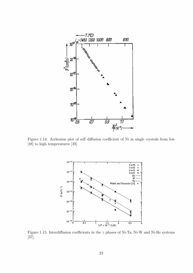
Figure 1.14: Arrhenius plot of self diffusion coefficient of Ni in single crystals from low[48] to high temperatures [49].

Figure 1.15: Interdiffusion coefficients in the γ phases of Ni-Ta, Ni-W and Ni-Re systems[37].

23

almost midway between Ta and Re. They attributed the difference in the interdiffusion

coefficients of Re, W and Ta in Ni to their diffusion pre-factors, while the derived activation

energies were very similar (see Equation (2.1) for definitions of diffusion pre-factors and

activation energies).

This however, is in stark contrast to the results obtained by Janotti et al [36] from

ab initio methods. They have systematically calculated the diffusion coefficients of tran-

sition metal solutes in Ni (Figure 1.16a), observing a similar trend as Karunaratne et al

[37]. However, they found that the activation energy barriers vary significantly amongst

different solutes in Ni (Figure 1.16b). Re (Atomic Number 75) was found to have the

highest activation energy barrier amongst all the solutes. This was also confirmed from

other ab initio works ([51], [52]). The experimental values for diffusion pre-factors and

activation energies are commonly obtained by fitting the diffusion data to the Arrhenius

relationship, and hence are prone to inconsistencies especially if the investigated temper-

ature range is small. On the other hand, these parameters are calculated directly in ab

initio methods. As a result, the experimental values may not be necessarily expected to

match the pre-factor and activation energy values obtained from ab initio methods.

Schuwalow et al [52] have calculated the vacancy diffusion coefficients for solutes in

Ni within dilute limits using a combination of ab initio calculations and kinetic Monte

Carlo simulations. Only one solute atom was considered in the simulation in the dilute

limit and vacancy jump barriers around it were accurately calculated. This eliminated

the possibility of any solute-solute interactions. The solute concentration was varied by

changing the size of the simulation cell, and the maximum possible solute concentration

was approximately 3 wt.% (about 0.9 at.%). The results showed a minimal influence of

the presence of solutes on vacancy diffusion, with a 3 wt.% Re addition slowing down

the vacancy diffusion by about 5% (Figure 1.17). They concluded that within the dilute

limits, interactions between the vacancies and solute atoms were too weak to have a net

effect at the relevant temperatures, but also suggested that consideration of solute-solute

interactions were necessary to account for the local fluctuations in solute concentration,

24

(a) Calculated diffusion coefficients for the 5d transition metals in Ni[36]

(b) Calculated activation energy barriers for the 5d transition metals in Ni[36]

Figure 1.16: Results from ab initio calculations of Janotti et al [36]

25

Figure 1.17: Vacancy diffusion coefficients for different concentrations of Re and Ta in Nias calculated by Schuwalow et al [52]

especially given the partitioning behaviour of solutes within the γ-γ′ structure.

26

CHAPTER 2

MODELLING DIFFUSION

The diffusion coefficient or diffusivity D is a phenomenological constant as defined from

Fick’s laws and is experimentally seen to follow the Arrhenius relationship,

D = D0 exp

{− Q

kBT

}(2.1)

where D0 and Q are the diffusion pre-factor and activation energy respectively, kB is

the Boltzmann constant and T is the absolute temperature.

However, diffusion is a stochastic process when looked at from an atomic level com-

pared to a deterministic process in a continuum medium. Random walk experiments are

developed to understand diffusion as an atomic scale process. For a sufficiently large num-

ber of independent random step sequences, the most probable or the root mean square

displacement of an atom for a random walk in any dimension is given as [53],

< |L|2 >1/2=√nλ (2.2)

where n is the number of steps and λ is the step length or the microscopic jump

distance. For the continuum case, considering the example of the release of a cloud of

diffusant particles from the origin, the most probable displacement as a function of time

t is given by [53],

27

< R2 >1/2=√

6Dt (2.3)

where D is the diffusion coefficient. If the time t in Equation (2.3) is associated with

the time required to execute n steps in Equation (2.2), we have,

D =1

6(n

t)λ2 (2.4)

Here, n/t is the step rate equivalent to the atomic jumping frequency, Γ. Thus, we

arrive at the Einstein′s formula [53],

D =1

6Γλ2 (2.5)

Thus, diffusion coefficient can be theoretically expressed in terms of microscopic pa-

rameters from solid-state principles [53]. The activation energy (Qi) and pre-factor (D0,i)

in Equation (2.1) can be expressed analytically using formulations as described later in

this chapter.

2.1 Modelling diffusion in dilute alloys

Analytical formulations are well established for the calculation of diffusion coefficients in

the dilute regime. The assumption is that the solute concentration is small such that the

solute atoms are always surrounded by the solvent (Ni) atoms and two solute atoms don’t

interact with each other in any way.

2.1.1 Calculation of self-diffusion and solute diffusion coefficients

In substitutional solid solutions, vacancy assisted diffusion is the dominant mechanism

for the movement of atoms which requires exchange of a vacancy with one of its nearest

neighbour atoms(see Figure 2.1). The solute diffusion coefficient (Di) for a solute i in

28

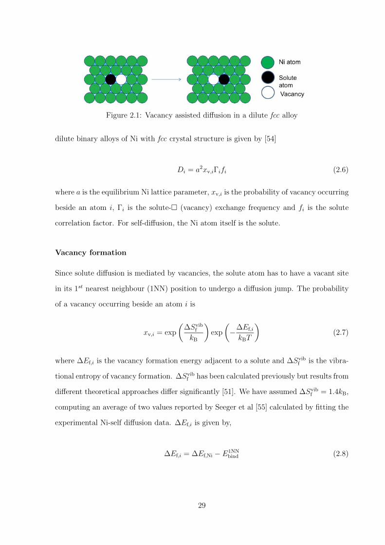
Figure 2.1: Vacancy assisted diffusion in a dilute fcc alloy

dilute binary alloys of Ni with fcc crystal structure is given by [54]

Di = a2xv,iΓifi (2.6)

where a is the equilibrium Ni lattice parameter, xv,i is the probability of vacancy occurring

beside an atom i, Γi is the solute-� (vacancy) exchange frequency and fi is the solute

correlation factor. For self-diffusion, the Ni atom itself is the solute.

Vacancy formation

Since solute diffusion is mediated by vacancies, the solute atom has to have a vacant site

in its 1st nearest neighbour (1NN) position to undergo a diffusion jump. The probability

of a vacancy occurring beside an atom i is

xv,i = exp

(∆Svib

f

kB

)exp

(−∆Ef,i

kBT

)(2.7)

where ∆Ef,i is the vacancy formation energy adjacent to a solute and ∆Svibf is the vibra-

tional entropy of vacancy formation. ∆Svibf has been calculated previously but results from

different theoretical approaches differ significantly [51]. We have assumed ∆Svibf = 1.4kB,

computing an average of two values reported by Seeger et al [55] calculated by fitting the

experimental Ni-self diffusion data. ∆Ef,i is given by,

∆Ef,i = ∆Ef,Ni − E1NNbind (2.8)

29

where ∆Ef,Ni is the vacancy formation energy in pure Ni. This is calculated from

∆Ef,Ni = E(NiN−1�)− N − 1

NE(NiN) (2.9)

where E(NiN) represents the total energy of a perfect supercell of Ni atoms and

E(NiN−1�) represents the energy when one of the atoms is replaced by a vacancy. N

is the number of atoms used in the energy calculations. E1NNbind is the binding energy

for a solute i and a vacancy at 1st nearest neighbour position to each other while being

surrounded by Ni atoms. This is given by[29],

E1NNbind = E(NiN−1i) + E(NiN−1�)− E(NiN−2(i−�)1NN)− E(NiN) (2.10)

where E(NiN−1i) represents the total energy of the supercell with a single solute atom

i, and E(NiN−2(i−�)1NN) represents the the total energy of the supercell with the solute

atom and a vacancy at 1st nearest neighbour position to each other.

Jump frequency

The jump frequency for a successful atom-� exchange is defined as [56]

Γi = ν∗i exp

{−∆Em,i

kBT

}(2.11)

where ν∗i is the effective frequency associated with the vibration of the atom in the direc-

tion of the vacancy [56] and ∆Em,i is the migration energy. For a successful atom-vacancy

exchange to take place, the atom has to push through a window of other atoms in the

vicinity, which requires local distortion of the lattice (see Figure (2.2)). The activation

energy associated with this process is known as the migration energy. It is the difference

between the energy at the saddle point (activated state) and the starting point of the

transition.

Within harmonic transition state theory, the effective frequency ν∗ is given as the

30

Figure 2.2: The atom-vacancy exchange showing an migration energy barrier

ratio of the product of 3N normal frequencies at the starting point of the transition to

the 3N -1 normal frequencies of the state constrained at the saddle point configuration,

N being the number of atoms in the system [56, 57],

ν∗ =

3N∏j=1

νj

3N−1∏j=1

ν′

j

(2.12)

Each atom has 3 degrees of freedom and is associated with 3 normal frequencies. So,

the entire crystal has 3N degrees of freedom x1, x2,..,x3N . These normal frequencies are

calculated from the second derivative matrix of energy or the force constant matrix β. β

is a 3N × 3N symmetric matrix (and hence is diagonalizable) whose ijth element is given

as[56],

βij =∂2E

∂xi∂xj(2.13)

Under harmonic approximation, the normal frequencies are the roots of the charac-

teristic equation[56] given as,

det[X − (2πν)2I] = 0 (2.14)

where, I is the unit matrix and the ijth element of X is βij/√mimj where mi and mj are

31

Figure 2.3: Various diffusion jumps in a dilute fcc alloy causing a vacancy-solute exchange,rotation and dissociation/association

the masses associated with the degrees of freedom xi and xj respectively.

Correlation factor

Correlation effects develop in a system as the atoms do not undergo a strict ‘random

walk’. The correlation factor fi gives a measure of this reduced efficiency of diffusion.

For self-diffusion in fcc crystals, a value of 0.78146 has been accurately determined using

computer simulations [58]. In dilute binary fcc alloys, several different jumps are possible

and fi is estimated using Lidiard’s model [59, 60, 61, 62]

fi =2Γrot + 7Γdis

2Γrot + 2Γi + 7Γdis

(2.15)

where Γrot and Γdis are jump frequencies for the rotation and dissociation of the solute-�

pair respectively, and Γi is the solute-� exchange frequency (see Figure 2.3).

32

Comparing the above Equations (2.6 - 2.15) with Equation (2.1), we can write

D0,i = fia2ν∗i exp

{∆Svib

f

kB

}(2.16)

Qi = ∆Ef,i + ∆Em,i (2.17)

. The values for the pre-factor (D0,i) and exponential terms (Qi) can be experimentally

determined from the slope and intercept of a graph of the logarithm of diffusivity versus

the inverse of temperature. These are commonly known as Arrhenius plots. Both D0,i and

Qi are assumed to be temperature independent. But while D0,i only affects the diffusivity

linearly, Qi has a much pronounced effect and thus even a small change in Qi can have

a big impact on diffusivity. It should be pointed out, however, that fi is not strictly

temperature independent, as it is in turn dependent on the values of Γi, Γdis and Γrot

which are temperature dependent. However, variation of fi with temperature is small in

most cases [63].

2.1.2 Calculation of vacancy diffusion coefficients

In the case of pure metals, one can calculate the vacancy diffusion coefficients by divid-

ing the self-diffusion coefficients by the equilibrium vacancy concentration at the same

temperature. However, in the case of alloys, the direct determination of vacancy diffu-

sion coefficients is less obvious using analytical formulations as other contributions come

in. Manning’s random alloy model [64] is the only available approximate method in the

literature to our best knowledge. This model applies to alloys where the atoms and va-

cancies are distributed randomly with no energetically favoured sites. Using this model,

the vacancy diffusion coefficient, Dv is given by

Dv = a2Γvfv (2.18)

33

where Γv is the average vacancy jump frequency and fv is the vacancy correlation factor.

The jump frequency of a vacancy is the same as the jump frequency of the atom exchanging

with the vacancy. In a binary alloy, Γv can be approximated by a simple arithmetic average

of the jump frequencies weighted by their respective atomic concentration,

Γv = xiΓi + xNiΓNi (2.19)

This approach assumes that the jump frequency of a given atom i, Γi, depends only on i

and not on the identity of other neighbouring atoms, and that the lattice site occupation

surrounding a vacancy is not biased relative to the average composition of the binary

alloy.

The vacancy follows a random walk in a pure crystal as all the vacancy jumps are

equally probable and hence fv is unity for the self-diffusion case. In a random alloy of Ni

where xi is the mole-fraction of solute i, fv is given by [64]

fv =xiΓif

iv + xNiΓNif

Niv

xiΓi + xNiΓNi

(2.20)

where f iv is the partial vacancy correlation factor for i. Since the correlation effect for

each component can differ, a partial vacancy correlation factor, f iv is defined for each

individual component i. The partial vacancy correlation factor, f iv is related to the solute

correlation factor, fi by equating the vacancy flux, Jv to the sum of the atom fluxes Ji

[64],

Jv =∑i

Ji (2.21)

The partial vacancy correlation factor, f iv enters into the direct calculation of Jv con-

sidering vacancy drift velocities, while the solute correlation factor, fi enters into the

calculation of Ji. Finally, f iv has been derived as [64]

34

f iv =fif0

(2.22)

where f0 is the correlation factor for self-diffusion in fcc crystals and is equal to 0.78146

[58]. For a detailed derivation of the Equation (2.22), one must refer to Manning’s work

[64]. Further, the general expression for the solute correlation factor, fi in any crystal

system with sufficient symmetry is given as [65],

fi =Hi

2Γi +Hi

(2.23)

where Hi is the effective escape frequency for the vacancies next to an atom of the

component i and determines whether a vacancy would undergo a subsequent reverse

exchange after a successful exchange with the atom i has taken place, thus introducing a

correlation effect. For the case of an fcc Ni crystal, Equation (2.23) simplifies to [64],

f0 =H0

2ΓNi +H0

(2.24)

Since f0 is a constant for pure fcc Ni crystals, this follows that the escape frequency

H0 would be directly proportional to ΓNi,

H0 = M0ΓNi (2.25)

where M0 is a numerical constant. Substituting the value of H0 from Equation (2.25)

into Equation (2.24), M0 is given as,

M0 =2f0

1− f0

(2.26)

Using a value of 0.78146 for f0 [58], a M0 value of 7.15 is obtained for fcc crystals.

Again, the relationship between the escape frequency Hi in a random alloy and H0 can

be approximated as [64]

35

Hi = fvH0 (2.27)

This is because the vacancy correlation is expected to affect the escape frequencies

in the same proportion as the vacancy diffusion rates. Substituting Equation (2.27) in

Equation (2.23), we get

fi =fvH0

2Γi + fvH0

(2.28)

Substituting Equation (2.20) and Equation (2.22) for fv and f iv, Equation (2.25) for

H0 and Equation (2.6) for Di, the solute correlation factor, fi for a random alloy can be

derived as [64],

fi = 1− 2Di

(M0 + 2)(xNiDNi + xiDi)(2.29)

and the vacancy correlation factor, fv for a random alloy can be derived as [64],

fv = 1− 2

M0

(M0 + 2)xNixi(DNi −Di)2

(M0 + 2)(xNiDNi + xiDi)2 − 2DNiDi

(2.30)

Note that the Manning’s random alloy model breaks down for dilute levels of solute

atoms which diffuse faster than the solvent, and we get negative values for the correlation

factors. This is because of the use of the various approximations in the model. Hence,

for these solutes, we have alternatively calculated fv from Equation (2.20), using Equa-

tion (2.22) for f iv. To a first approximation, the partial vacancy correlation factor for Ni,

fNiv is taken as unity for the case of dilute alloys.

2.2 Kinetic Monte Carlo simulations

Computer simulations are widely used to model materials at the atomic level. The mod-

elled systems may contain up to many thousands of atoms, and hence it is possible to

sample a wide configurational space. The exact positions of the atoms are tracked and

36

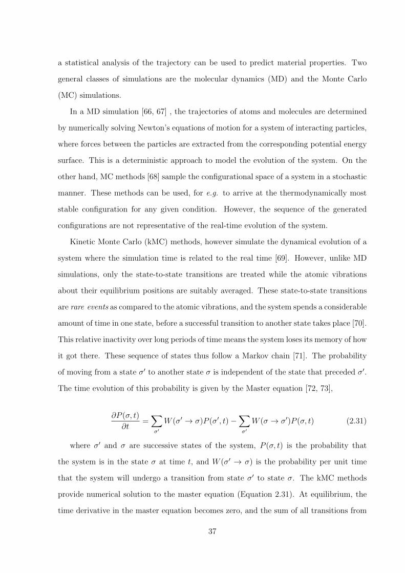
a statistical analysis of the trajectory can be used to predict material properties. Two

general classes of simulations are the molecular dynamics (MD) and the Monte Carlo

(MC) simulations.

In a MD simulation [66, 67] , the trajectories of atoms and molecules are determined

by numerically solving Newton’s equations of motion for a system of interacting particles,

where forces between the particles are extracted from the corresponding potential energy

surface. This is a deterministic approach to model the evolution of the system. On the

other hand, MC methods [68] sample the configurational space of a system in a stochastic

manner. These methods can be used, for e.g. to arrive at the thermodynamically most

stable configuration for any given condition. However, the sequence of the generated

configurations are not representative of the real-time evolution of the system.

Kinetic Monte Carlo (kMC) methods, however simulate the dynamical evolution of a

system where the simulation time is related to the real time [69]. However, unlike MD

simulations, only the state-to-state transitions are treated while the atomic vibrations

about their equilibrium positions are suitably averaged. These state-to-state transitions

are rare events as compared to the atomic vibrations, and the system spends a considerable

amount of time in one state, before a successful transition to another state takes place [70].

This relative inactivity over long periods of time means the system loses its memory of how

it got there. These sequence of states thus follow a Markov chain [71]. The probability

of moving from a state σ′ to another state σ is independent of the state that preceded σ′.

The time evolution of this probability is given by the Master equation [72, 73],

∂P (σ, t)

∂t=∑σ′

W (σ′ → σ)P (σ′, t)−∑σ′

W (σ → σ′)P (σ, t) (2.31)

where σ′ and σ are successive states of the system, P (σ, t) is the probability that

the system is in the state σ at time t, and W (σ′ → σ) is the probability per unit time

that the system will undergo a transition from state σ′ to state σ. The kMC methods

provide numerical solution to the master equation (Equation 2.31). At equilibrium, the

time derivative in the master equation becomes zero, and the sum of all transitions from

37

Figure 2.4: Contour plot showing an atom vibrating at its equilibrium position, and arare diffusive jump by surmounting of the energy barrier [70]

σ′ to σ equals the sum of all transitions from σ to σ′ [72, 73],

W (σ′ → σ)Peq(σ′) = W (σ → σ′)Peq(σ) (2.32)

where Peq denotes the equilibrium probability. This is called the detailed-balanced

criterion [72, 73], and this needs to be fulfilled for the system to attain thermal equilibrium.

Diffusive exchange between an atom and a vacancy is a typical example of a rare

event. At a finite temperature, the atoms vibrate about their mean positions (typically

once every 10−12 s) [69]. Occasionally an atom surrounding a vacancy can surmount

the energy barrier and exchange its position with a vacancy (see Figure 2.4). However

these diffusion jumps are rare, and happen on a higher time scale (typically ≈ 10−6 s)

[69]. An accurate integration in an MD simulation would require time steps short enough

to resolve atomic vibrations and hence the total simulation time is restricted. Thus, it

is computationally unfeasible to study the problem of diffusion using MD simulations.

This problem is solved using the kMC method, as it concentrates only on the rare event

of diffusion. Thus, much larger time scales can be reached in a kMC simulation when

compared to the MD simulations.

The algorithm for a kMC simulation to calculate the diffusion coefficients is as follows

[74] :

38

1. Set up the fcc lattice and populate it with atoms leaving one site empty representing

a vacancy. Fix the temperature at the desired value T and set time t=0.

2. Calculate all the jump frequencies Γ1,Γ2,...,Γ12 (see Equation (2.11)) corresponding

to the possible vacancy jumps at this state. In an fcc crystal, a vacancy can exchange

its position with atoms on its 12 nearest neighbour sites. Hence, the number of

possible vacancy jumps is 12 at each state.

3. Calculate the cumulative sum Γi =∑i

j=1 Γj for each vacancy jump i = 1, 2, ..., 12.

4. Generate a uniform random number ρ1 ∈ (0,1].

5. Find the vacancy jump to carry out by finding the i for which

Γi−1 < ρ1Γ12 ≤ Γi.

6. Carry out the vacancy jump i.

7. Generate another uniform random number ρ2 ∈ (0,1].

8. Update time t = t + ∆t where ∆t = − ln ρ2

Γ12. This is because the kMC algorithm

simulates a Poisson process, and a relationship with the real time can thus be

established [73].

9. The system has moved to a new state after the vacancy jump. Repeat steps 2

through 8 for the desired number of vacancy jumps.

10. Track the atoms and the vacancy coordinates throughout the simulation. At the end

of the desired number of vacancy jumps, calculate the vacancy diffusion coefficient

Dv for a single vacancy using

Dv =1

6

∂

∂t

⟨R2

v(t)⟩

(2.33)

and the solute diffusion coefficient using

39

Di =xv

xsimv

× 1

6N

∂

∂t

N∑i=1

⟨[R2i (t)]⟩

(2.34)

where 〈R2(t)〉 is the mean square displacement of the vacancy (or solute atoms)

from the initial state, N is the number of i atoms and t is the time elapsed. xv is

the actual vacancy concentration at temperature = T (see Equation (2.7)), while

xsimv is the vacancy concentration used in the kMC simulation. R2(t) is calculated

as

R2(t) = |x(t)− x(0)|2 + |y(t)− y(0)|2 + |z(t)− z(0)|2 (2.35)

where the values on the right represent the coordinates of the vacancy(or solute

atoms) at time = t and time = 0.

The kMC simulation should be run for a sufficiently large number of steps such

that the D values converge. To obtain better statistics, the kMC trajectory can be

divided over a number of segments and D can be calculated from the time-weighted

averages of the diffusion coefficients calculated from the various segments [52, 75].

2.3 Modelling diffusion in non-dilute alloys

Analytical methods for the rigorous calculation of diffusion coefficients in non-dilute alloys

cannot be formulated given the complexity of the problem, however some approximate

models do exist in the literature [51, 76, 77, 78] . For the case of dilute alloys, only a

few activation energy barriers are needed to describe the system. However in the case of

non-dilute alloys, atoms can be arranged in a number of configurations. This means a

number of activation energy barriers corresponding to these atomic configurations need

to be calculated, which is difficult. Further, to calculate these energy barriers, one needs

to calculate both the energy of the activated state and the energy of the end states. This

problem is made simpler by using the cluster expansion method which is described below.

We have dealt with the binary Ni-Re system in the non-dilute regime.

40

Figure 2.5: A 2D lattice showing some possible clusters

2.3.1 Cluster expansion method

The cluster expansion can be seen as a generalised Ising Model [79] . The lattice of a

binary alloy such as Ni-Re can be represented using occupation variables (σi) [80, 81, 82].

A value of +1 represents a Ni atom, while -1 represents a Re atom. The vector of the

occupation variables ~σ would then uniquely describe the configuration of the system. The

energy of the alloy E for a configuration ~σ can be expanded using polynomials φα of (σi)

E(~σ) = V0 +∑α

Vαφα(~σ) (2.36)

where φα is simply the product of occupation variables belonging to a particular clus-

ter of sites α , i.e. φα =∏

i∈α σi . These clusters could be point clusters, pairs, triplets,

quadruplets. . . etc (see Figure 2.5). The expansion of this equation to an infinite num-

ber of clusters theoretically should describe the energy exactly. However, the expansion

is usually truncated up to a few clusters which can describe the energy to a reasonable

precision. Vα are the Effective Cluster Interaction (ECI) coefficients and are calculated

by fitting energy calculated from first principles (see Chapter 3) for a number of config-

urations [83]. Thus, from a relatively small first principles dataset, the energy for any

given configuration can be cluster expanded using this technique.

41

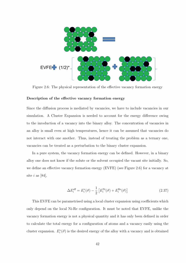
Figure 2.6: The physical representation of the effective vacancy formation energy

Description of the effective vacancy formation energy

Since the diffusion process is mediated by vacancies, we have to include vacancies in our

simulation. A Cluster Expansion is needed to account for the energy difference owing

to the inroduction of a vacancy into the binary alloy. The concentration of vacancies in

an alloy is small even at high temperatures, hence it can be assumed that vacancies do

not interact with one another. Thus, instead of treating the problem as a ternary one,

vacancies can be treated as a perturbation to the binary cluster expansion.

In a pure system, the vacancy formation energy can be defined. However, in a binary

alloy one does not know if the solute or the solvent occupied the vacant site initially. So,

we define an effective vacancy formation energy (EVFE) (see Figure 2.6) for a vacancy at

site i as [84],

∆Eeffi = Ev

i (~σ)− 1

2

[ENii (~σ) + ERe

i (~σ)]

(2.37)

This EVFE can be parametrised using a local cluster expansion using coefficients which

only depend on the local Ni-Re configuration. It must be noted that EVFE, unlike the

vacancy formation energy is not a physical quantity and it has only been defined in order

to calculate the total energy for a configuration of atoms and a vacancy easily using the

cluster expansion. Evi (~σ) is the desired energy of the alloy with a vacancy and is obtained

42

by rearranging Equation (2.37). ENii (~σ) and ERe

i (~σ) are the energies when the vacancy is

replaced by a Ni atom or a Re atom, and these can be calculated from the usual binary

cluster expansion.

Calculation of kinetically resolved activation energy barriers

The activation energy barriers not only depend on the surrounding configuration, but also

on the direction of the jump. Hence to get around this, kinetically resolved activation

(KRA) barriers are defined as [85],

∆EKRA = Es −1

2(Ei + Ef ) (2.38)

where Es is the energy of the activated state (saddle point), while Ei and Ef are the

energy of the initial state and the final state (2 end points) of the jump (see Figure 2.7).

∆EKRA is thus independent of the direction of the hop, and can be cluster expanded

locally using a formalism similar to EVFE,

∆EKRA = K0 +∑α

Kαφα (2.39)

where Kα are Kinetic Effective Cluster Interaction coefficients (KECIs) to describe

KRAs as a function of configuration. Once the KRAs and the energies of the end states

are available, the activation energy barriers ∆Ea can be calculated as,

∆Ea = Es − Ei = ∆EKRA +1

2(Ef − Ei) (2.40)

Thus the cluster expanded energy of the binary alloy, the EVFE and the KRAs to-

gether would describe the Ni-Re system completely. These numbers are then fed into the

kMC simulation to calculate the vacancy diffusion coefficients in the non-dilute regime.

43

Figure 2.7: A schematic diagram illustrating the meaning of the kinetically resolvedactivation energy barriers

44

CHAPTER 3

COMPUTING ENERGIES

It follows from the previous chapter that diffusivity in dilute and non-dilute binary systems

can be modelled using different methods, provided that the energetics of the system are

known. Density functional theory (DFT) [86, 87] is currently the best technique to obtain

the defect and migration energies required for this work accurately and within reasonable

computational time. This chapter will cover some background of DFT, details of the

calculations carried out, and methods used to calculate the migration barriers.

3.1 Density functional theory

DFT is often referred to as belonging to the group of first principles or ab initio techniques.

Ab initio calculations are named so because they are completely based on quantum me-

chanical theoretical principles and use no input from experiments. In this context, DFT

is a feasible approach to finding solutions to the Schrodinger equation, the fundamen-

tal equation that describes the quantum behaviour of atoms and molecules. Solving the

Schrodinger equation for a complex system such as the ones treated within this work is

computationally impossible, and DFT provides a way to make the problem tractable. In

order to do this, DFT employs several approximations, which are described within this

section.

The first approximation, which is common to many first-principles methods, separates

45

the description of the motion of the nuclei from the description of the motion of the

electrons (theBorn−Oppenheimer approximation) [88]. This approximation is applicable

because of the large mass difference between the nuclei and the electrons. Due to this

difference in mass, the nuclei move much slower than the electrons which means they can

be considered stationary when solving the electronic part of the Schrodinger equation. As

a result, the Schrodinger equation can be written as

[−~2

2m

N∑i=1

∇2i +

N∑i=1

V (ri) +N∑i=1

∑j<i

U(ri, rj)

]ψ = Eψ (3.1)

where, the first term on the LHS represents the kinetic energy of each electron, the second

term represents the interaction energy between each electron and the collection of nuclei,

and the third term represents the interaction energy between different electrons. E is the

ground state energy of the electrons and ψ(r1, r2, ..., rN) is the electronic wave function,

where r1, r2, ..., rN are the spatial coordinates of each of the N electrons. Thus, solving

for ψ becomes a many-body problem, as the individual wave function ψi(r) cannot be

determined without simultaneously considering the individual wave functions associated

with all the other electrons and it becomes more and more difficult to solve the equation

as the size of the system increases.

This is where the theorems formulated by Hohenberg and Kohn can help us find a

solution to the many-body Schrodinger equation. The first theorem by Hohenberg and

Kohn [86] states that the electronic ground state energy could be expressed as a functional

of the electron density, n(r). This can be summarised as

E = E[n(r)] (3.2)

where,

n(r) = 2∑i

ψ∗i (r)ψi(r) (3.3)

The second theorem states that the electron density which minimises the energy func-

46

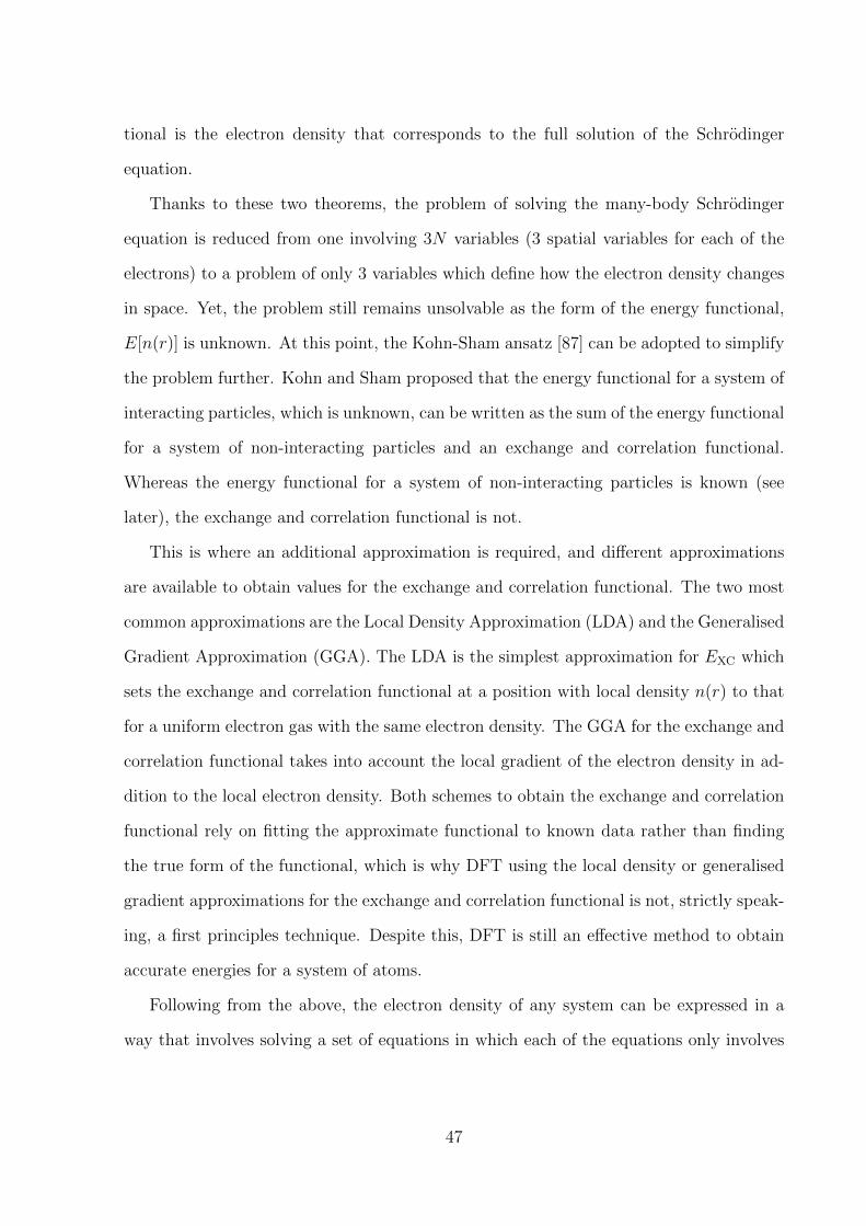
tional is the electron density that corresponds to the full solution of the Schrodinger

equation.

Thanks to these two theorems, the problem of solving the many-body Schrodinger

equation is reduced from one involving 3N variables (3 spatial variables for each of the

electrons) to a problem of only 3 variables which define how the electron density changes

in space. Yet, the problem still remains unsolvable as the form of the energy functional,

E[n(r)] is unknown. At this point, the Kohn-Sham ansatz [87] can be adopted to simplify

the problem further. Kohn and Sham proposed that the energy functional for a system of

interacting particles, which is unknown, can be written as the sum of the energy functional

for a system of non-interacting particles and an exchange and correlation functional.

Whereas the energy functional for a system of non-interacting particles is known (see

later), the exchange and correlation functional is not.

This is where an additional approximation is required, and different approximations

are available to obtain values for the exchange and correlation functional. The two most

common approximations are the Local Density Approximation (LDA) and the Generalised

Gradient Approximation (GGA). The LDA is the simplest approximation for EXC which

sets the exchange and correlation functional at a position with local density n(r) to that

for a uniform electron gas with the same electron density. The GGA for the exchange and

correlation functional takes into account the local gradient of the electron density in ad-

dition to the local electron density. Both schemes to obtain the exchange and correlation

functional rely on fitting the approximate functional to known data rather than finding

the true form of the functional, which is why DFT using the local density or generalised

gradient approximations for the exchange and correlation functional is not, strictly speak-

ing, a first principles technique. Despite this, DFT is still an effective method to obtain

accurate energies for a system of atoms.

Following from the above, the electron density of any system can be expressed in a

way that involves solving a set of equations in which each of the equations only involves

47

a single electron [87].

[−~2

2m∇2 + V (r) + VH(r) + VXC(r)

]ψi(r) = εiψi(r) (3.4)

In Equation (3.1), the potential V defines the interaction between an electron and the

collection of atomic nuclei and VH, or the Hartree potential, represents the Coulombic

repulsion between the electron being considered and the net electron density [88]. This

latter term also includes a self- interaction, as the electron being considered is also a part

of the net electron density. This interaction is unphysical and the correction for it is one

of the several effects which are lumped together in the potential term VXC. VXC can be

formally expressed as a functional derivative of the exchange and correlation energy.

Now, to solve the Kohn-Sham equations, we need to define the Hartree potential,

and to define the Hartree potential we need to know the electron density. But to find

the electron density, we must know the single-electron wave functions, and to know these

wave functions we must solve the Kohn-Sham equations. To break this circle, the problem

is usually treated in an iterative way where an initial trial electron density is defined.

Progressively, this trial density is updated until it matches the calculated electron density.

Thus, this iterative method leads to a solution that is self-consistent.

The Kohn-Sham equations [87] can be solved using plane wave basis sets. However

the disadvantage is that we require large number of plane waves to expand the wave

functions in the core region, because the wave functions of the core electrons are highly

localized and oscillating. This problem can be solved by the usage of pseudopotentials

[89, 90]. Here the numerical problems associated with the electron-ion interaction are

eliminated. The chemically inert core electrons are not considered in the calculations and

since only the valence electrons are involved, the problem is simpler. Pseudopotentials

are often described by their softness, or the kinetic energy cutoff value required to achieve

accurate results. Several schemes have been formulated to increase the softness of pseu-

48

dopotential, leading to ultra-soft pseudopotentials (USPPs). These schemes, however,

rely on parameters which render the USPPs less portable across different systems. Some

of these issues are solved using the projector augmented wave (PAW) method [91]. PAW

pseudo-potentials are often considered superior to USPPs due to the fact they are more

transferable and lead to more accurate spin-polarised calculations.

3.2 Nudged elastic band method

The Nudged Elastic Band method [92] was employed to identify the saddle points for the

atom-� exchanges and to calculate the activation energy barriers. The transition from one

stable configuration to another takes place along the minimum energy path (MEP) and

the difference in the saddle point energy or the energy maximum along the MEP and the

initial energy is the activation energy barrier. If one considers the multidimensional energy

landscape (see Figure 3.1), a stable configuration is a local minimum, while a saddle point

refers to a ‘minimax’ (maximum along the MEP). Mathematically, the second derivative

of a local minima has all positive eigenvalues, while that for a saddle point has exactly

one negative eigenvalue. Thus, from the second derivative test, the saddle point can be

traced. However, this method would require the evaluation and diagonalization of the

second derivative of energy at each step which for a large system with many dimensions

(degrees of freedom) is exceedingly difficult.

The plain elastic band method [93] on the other hand requires only the first derivative

of the energy. Several states (or ‘images’) are interpolated between the known end states

and these are connected by imaginary spring forces. The object function is defined as,

SPEB(~R1, . . . , ~RP−1) =P∑i=0

V (~Ri) +P∑i=1

Pk

2(~Ri − ~Ri−1)2 (3.5)

where i = 0, 1, . . . , P represent the images, Ri represent the position coordinates, ki

represent the spring constants and V represents the potential energy. The force acting

on an image i is given as the sum of the gradient of the potential energy and the spring

49

Figure 3.1: The initial and final configurations in a 2-D energy landscape using NEBmethod with 16 images. The initial linearly interpolated configuration finally convergesto the MEP [93]

force,

~Fi = −~∇V (~Ri) + ~F Si (3.6)

where

~F Si ≡ ki+1(~Ri+1 − ~Ri)− ki(~Ri − ~Ri−1) (3.7)

The initial configuration of images is updated according to the forces acting on the

images. However, the plain elastic band also fails in certain cases as shown in Figure 3.2.

A higher spring constant holds the image too tightly and hence results in corner cutting

or an overestimate of the barrier energy. While, if the spring constant is low, the images

slide down towards the end points and hence decrease the resolution near the saddle point.

The corner cutting is caused by the perpendicular component of the spring force, while

the sliding down is caused by the component of the true force ~∇V (Ri) in the direction of

the path. These forces are projected out in a nudged elastic band method[93], and hence

50

Figure 3.2: The plain elastic band results for a case with a curved path near the saddlepoint (a) k=1.0, and (b) k=0.1. The result for a NEB is shown by a solid line which goesthrough the saddle point [93].

the force on an image becomes the sum of the perpendicular component of the true force

and the parallel component of the spring force,

~F 0i = −~∇V (Ri)|⊥ + ~F S

i .τ‖τ‖ (3.8)

Here τ‖ is the unit tangent along the path. This action is known as ‘nudging’ and the

method always converges to the MEP, provided sufficient number of images are used in

the calculations. Since the spring force only decides the separation between the images,

the choice of a spring constant becomes arbitrary[93]. The NEB method can be efficiently

run on parallel system of computers with each node handling a single image. A ‘climbing

image’ NEB [92] is a small modification to the NEB where one of the images is pushed

to the exact saddle point, thus making the identification of the saddle point easier.

3.3 Settings for calculations

All input data were calculated from first principles, using DFT [86, 87] as implemented

in the Vienna Ab initio simulation package (VASP) 5.3.2 [94]. The projector augmented

wave (PAW) method [91, 95] was used to describe the electron-ion interactions, and the

generalized gradient approximation (GGA) parameterised by Perdew, Burke and Ernzer-

hof [96] was used as EXC. The PAW method was adopted due to its transferability, and

51

the fact that it has been shown to be more accurate in spin-polarised systems [88]. The

GGA was used to approximate the exchange and correlation functional as it has been

shown to estimate migration barriers and lattice parameters more accurately [88].

All calculations were spin-polarized. Pure Ni is ferromagnetic below 627 K. As a result,

it was deemed appropriate for all calculations used in this work to be spin-polarized. Test

calculations were carried out both with and without spin-polarization. It was revealing

to see a dramatic difference in Re-Re binding energy within the Ni fcc lattice depending

on whether calculations were spin-polarized or non-spin-polarized. This will be discussed

in the context of the results in Chapter 5.

The electronic self-consistent loops were stopped when the total energy converged to

within 10−6 eV and ionic positions were relaxed until all forces fell below 10−2 eV/A. The

conjugate-gradient algorithm was used to relax the atoms in to their instantaneous ground

states. A Methfessel-Paxton smearing width [97] of 0.1 eV was used. The migration

barriers were calculated using the ‘climbing image’ nudged elastic band method [98, 92]

using a maximum of 5 images. A spring constant value of 5 eV/A2 was used. The effective

frequencies were calculated within the harmonic approximation as supported by VASP.

The cluster expansion was performed using the CASM code (Cluster-Assisted Sta-

tistical Mechanics) developed by the Van der Ven Research Group at the University of

Michigan [81, 82].

3.4 Convergence tests

In each numerical approximation within DFT, it is possible to find a solution that is closer

to the exact solution by using more computational resources. As computational time is

not unlimited, however, we must ensure we restrict ourselves to our required accuracy. A

‘well-converged’ solution is one where we get accurate results, but not at the expense of

unnecessarily high computational time. In DFT calculations, computational parameters,

most notably the quality of plane wave basis sets (defined by the energy cutoff) and the

52

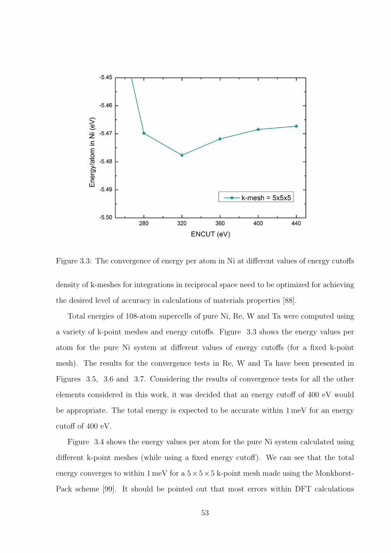
Figure 3.3: The convergence of energy per atom in Ni at different values of energy cutoffs

density of k-meshes for integrations in reciprocal space need to be optimized for achieving

the desired level of accuracy in calculations of materials properties [88].

Total energies of 108-atom supercells of pure Ni, Re, W and Ta were computed using

a variety of k-point meshes and energy cutoffs. Figure 3.3 shows the energy values per

atom for the pure Ni system at different values of energy cutoffs (for a fixed k-point

mesh). The results for the convergence tests in Re, W and Ta have been presented in

Figures 3.5, 3.6 and 3.7. Considering the results of convergence tests for all the other

elements considered in this work, it was decided that an energy cutoff of 400 eV would

be appropriate. The total energy is expected to be accurate within 1 meV for an energy

cutoff of 400 eV.

Figure 3.4 shows the energy values per atom for the pure Ni system calculated using

different k-point meshes (while using a fixed energy cutoff). We can see that the total

energy converges to within 1 meV for a 5×5×5 k-point mesh made using the Monkhorst-

Pack scheme [99]. It should be pointed out that most errors within DFT calculations

53

Figure 3.4: The convergence of energy per atom in Ni with different k-point densities

are systematic, and that energy differences converge faster with respect to the precision

adopted for the various numerical approximations.

Further discussion on the convergence of NEB calculations particularly with respect

to the supercell size has been presented in Section 4.1.4.

54

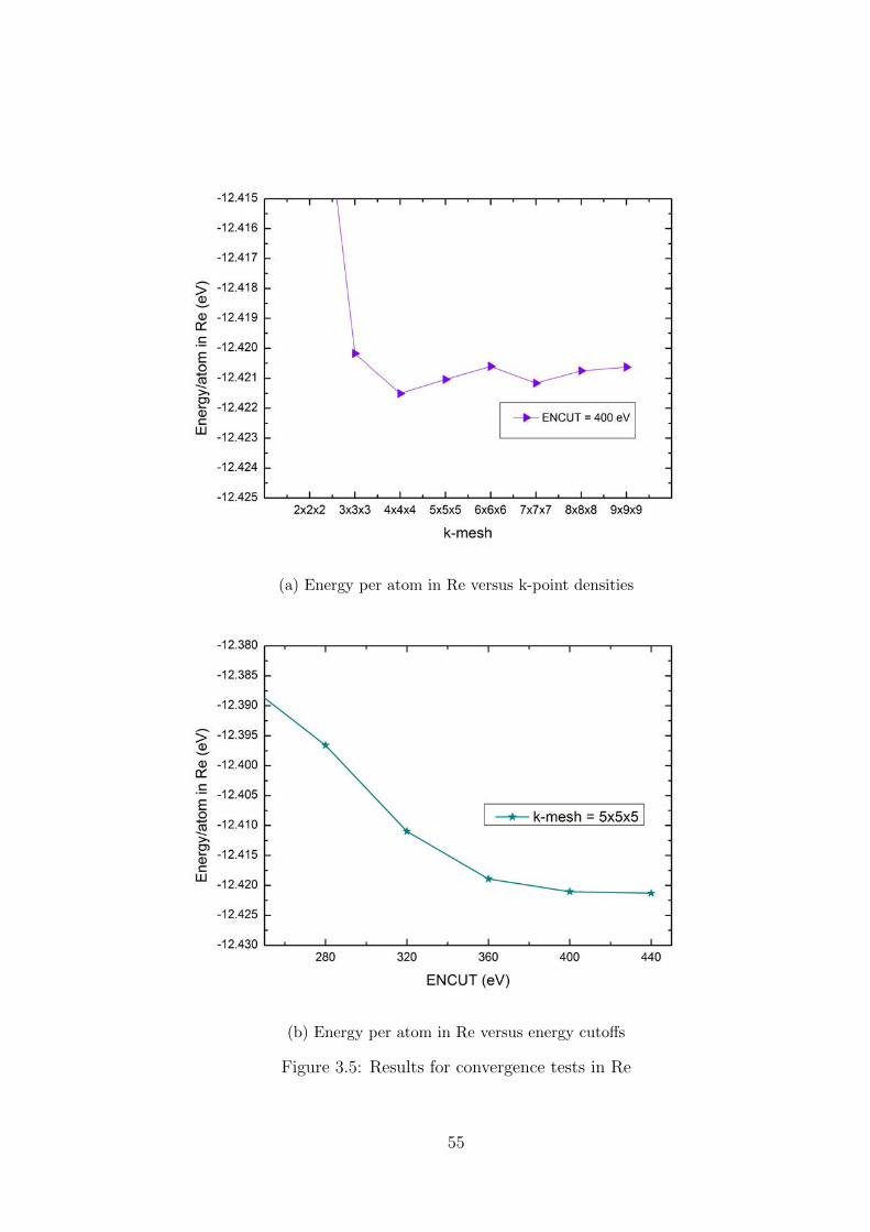
(a) Energy per atom in Re versus k-point densities

(b) Energy per atom in Re versus energy cutoffs

Figure 3.5: Results for convergence tests in Re

55

(a) Energy per atom in W versus k-point densities

(b) Energy per atom in W versus energy cutoffs

Figure 3.6: Results for convergence tests in W

56

(a) Energy per atom in Ta versus k-point densities

(b) Energy per atom in Ta versus energy cutoffs

Figure 3.7: Results for convergence tests in Ta

57

CHAPTER 4

DIFFUSION IN DILUTE ALLOYS

4.1 Results from analytical expressions

All the calculated values from Equation (2.6) have been presented in the following sections.

For nudged elastic band calculations, only the internal degrees of freedom of the supercells

were relaxed and the supercell size was fixed to that calculated for pure Ni. The total

energies change only by about ± 0.03 eV when the supercell volume and shape relaxations

were taken into account. For all other calculations, besides the internal degrees of freedom

of the supercells, the volume and the shape of the supercells were relaxed as well. Most

of the remaining details of the computational setup are mentioned in Section 3.3. Further

details about particular calculations have been discussed in their respective sections.

4.1.1 Lattice parameters and local relaxation around defects

The relaxed volume for a 3×3×3 supercell of pure Ni corresponded to a lattice parameter

value, a of 3.52 A, which fits well with the experimental Ni lattice parameter of 3.524 A

[100]. In order to calculate the change in the macroscopic lattice parameter (∆a) on the

introduction of a defect, the corresponding defect was introduced in the 3×3×3 supercell

of Ni, replacing one of the Ni atoms. For a vacancy, a decrease of 0.005 A was calculated

for the macroscopic lattice parameter, while for the cases of Re, W and Ta an increase

58

Table 4.1: The calculated change in the macroscopic lattice parameter (∆a) and thepercentage local relaxation for a vacancy and for Re, W and Ta in Ni

Defect ∆a (A) % relaxation

Vacancy -0.005 -1.56

Re 0.002 0.370.0036 [101] 0.27 [29]

W 0.003 0.700.0038 [101] 0.63 [29]

Ta 0.005 1.800.0054 [101] 1.51 [29]

of 0.002 A, 0.003 A and 0.005 A respectively was calculated for the same. These values

were consistent with the theoretical work of Wang et al [101] (see Table 4.1).

The results for the introduction of the defect on the local relaxation in the 1st nearest

neighbour distance between the defect and a Ni atom in reference to the 1st nearest

neighbour distance between two Ni atoms in a pure Ni supercell have been tabulated in

Table 4.1. For the case of a vacancy, the 1st nearest neighbour distance reduces to 1.56

%. This is because the 1st nearest neighbour shell of Ni atoms around a vacancy will be

pushed inwards owing to the net compressive stress from the Ni atoms surrounding the

shell. On the other hand, the introduction of all the solute atoms tend to push the 1st

nearest neighbour shell of atoms outwards thereby producing a positive local strain. The

calculated values were 0.37 % for Re, 0.70 % for W and 1.80 % for Ta respectively, and

these values match well with the results of Mottura et al [29]. This is expected given the

atomic radii of Re, W and Ta are 1.97 A, 2.02 A and 2.09 A respectively when compared

to 1.62 A for Ni [29]. However, the size misfit does not completely describe the magnitude

of local relaxation and the electronic effects must also be considered. It can be inferred

that Re, in comparison to W and Ta, forms a stronger directional bond with the Ni atoms,

thus leading to a smaller expansion in nearest neighbour distance.

59

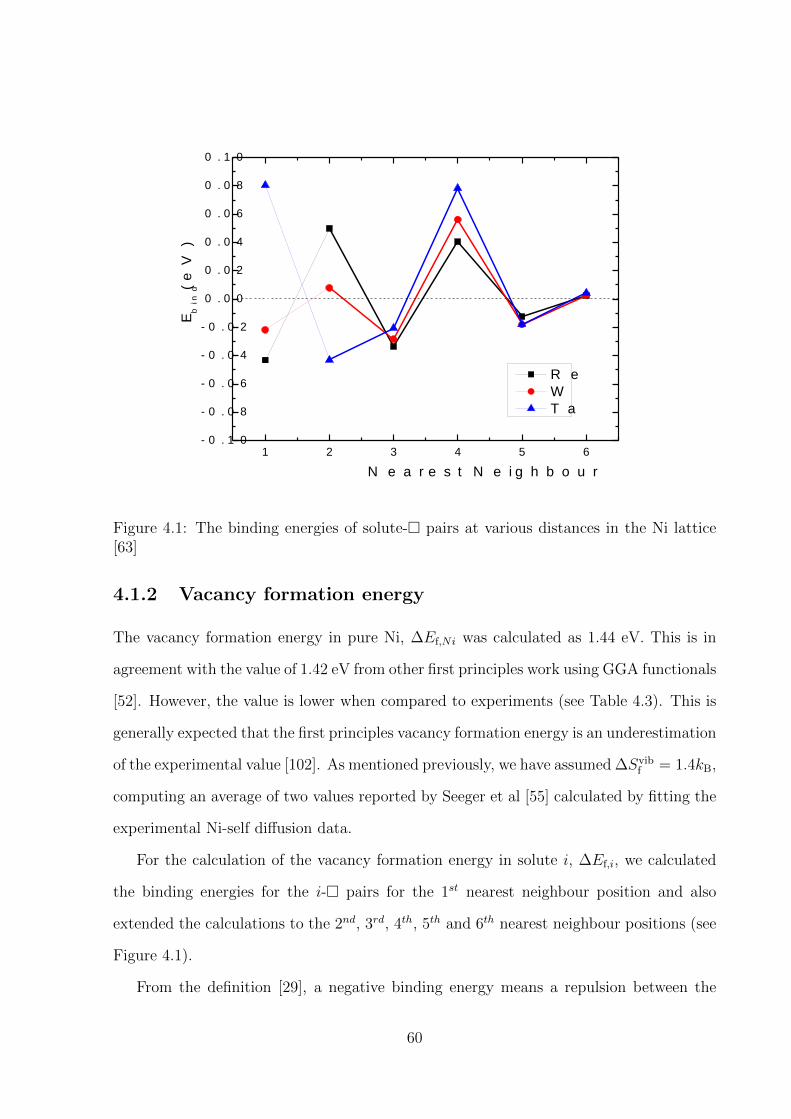
1 2 3 4 5 6- 0 . 1 0- 0 . 0 8- 0 . 0 6- 0 . 0 4- 0 . 0 20 . 0 00 . 0 20 . 0 40 . 0 60 . 0 80 . 1 0

E bind (e

V)

N e a r e s t N e i g h b o u r

R e W T a

Figure 4.1: The binding energies of solute-� pairs at various distances in the Ni lattice[63]

4.1.2 Vacancy formation energy

The vacancy formation energy in pure Ni, ∆Ef,Ni was calculated as 1.44 eV. This is in

agreement with the value of 1.42 eV from other first principles work using GGA functionals

[52]. However, the value is lower when compared to experiments (see Table 4.3). This is

generally expected that the first principles vacancy formation energy is an underestimation

of the experimental value [102]. As mentioned previously, we have assumed ∆Svibf = 1.4kB,

computing an average of two values reported by Seeger et al [55] calculated by fitting the

experimental Ni-self diffusion data.

For the calculation of the vacancy formation energy in solute i, ∆Ef,i, we calculated

the binding energies for the i-� pairs for the 1st nearest neighbour position and also

extended the calculations to the 2nd, 3rd, 4th, 5th and 6th nearest neighbour positions (see

Figure 4.1).

From the definition [29], a negative binding energy means a repulsion between the

60

vacancy and the solute atom. We can see that the binding energies differ greatly between

the three solutes in the first two nearest neighbour positions. For the 1st nearest neighbour

position, Re and W show values of -0.04 eV and -0.02 eV respectively for the binding

energy, while Ta shows a value of +0.08 eV. This means that Ta prefers a vacancy on

its 1st nearest neighbour position, while Re and W do not. The presence of the vacancy

affects the bonding between the solute and the Ni atoms. This can be referred to as

the electronic effect and it is stronger when the vacancy is relatively close to the solute

atom. The change from an attractive binding energy in Ta to repulsive binding energies

in W and Re can be attributed to the increased band filling from Ta to W and Re. The

results agree with the work of Schuwalow et al [52]. However, these interactions are weak,

considering their magnitude. Also, one can see that from 3rd nearest neighbour position

onwards, the behaviour of all the three solutes become similar and finally the binding

energies vanish at the 6th nearest neighbour position. Here the elastic effects due to the

size mismatch of the solute and host Ni dominate the electronic effects and hence all the

solutes show similar behaviour. The ∆Ef,Ni value and the ∆Ef,i values for Re, W and Ta

are tabulated in Table 4.3.

4.1.3 Effective frequencies

The lattice dynamics, as supported by VASP allows to calculate the Hessian matrix, or

the second derivative of the energy with respect to the atomic positions and hence the

vibrational frequencies of a system. The calculation of the full Hessian of all the atoms

in the supercell is computationally intensive. Hence, these calculations were performed

for a single Ni, Re, W and Ta atom which undergo a vacancy exchange at the initial and

the saddle point of the transition. This simplification has been used previously [36, 103]

as well. Each atom is displaced in x, y and z directions by a small positive and negative

displacement (0.015 A) and from the forces, the Hessian matrix is calculated.

Table 4.2 shows the three normal frequencies calculated at the initial point of the

transition, the two normal frequencies at the saddle point (one frequency at the saddle

61

Table 4.2: The calculated effective frequencies for Ni, Re, W and Ta

Solute Vibrational frequencies at Vibrational frequencies at ν∗ithe initial point(THz) the saddle point(THz) (THz)

Niself 6.03 5.99 5.10 10.14 7.06 2.574.48 [103]

Re 4.30 4.14 3.53 7.25 5.17 1.67W 4.52 4.36 3.78 6.74 4.69 2.36Ta 4.48 4.38 3.70 6.18 4.59 2.56

point is imaginary (see Equation (2.12)) and the calculated effective frequency ν∗. It must

be noted that the calculated effective frequencies are in the range of tera Hertz (1012 Hz),

showing how vigorously the atoms vibrate about their mean positions in a crystal lattice.

A ν∗ value of 2.57 THz was calculated for the case of Ni, as compared to a value of 4.48

THz calculated by Tucker et al [103] from their first principles work. The ν∗ values of

Re, W and Ta differ slightly, but are in the same approximate range. Given the similar

masses of the three solutes, the differences in their calculated frequencies are related

almost entirely to the calculated Hessian matrix (see subsection 2.1.1), which in turn is

related to the energy landscapes at the initial and the saddle points of the transition. All

the three solutes are expected to have similar energy landscapes at the initial points of

the transition as implied from the calculated vibrational frequencies at the initial points.

However, at the saddle point, Re exhibits higher vibrational frequencies compared to W

and Ta, leading to a smaller ν∗ value. This implies that a small displacement of a Re

atom from its saddle point would lead to a higher penalty in the energy as compared to

that of a W or a Ta atom. The ν∗ values of Re, W and Ta have been calculated by Janotti

et al [36] but have not been explicitly reported, and hence a comparison was not possible.

4.1.4 Migration energy barriers

A 3×3×3 supercell of Ni atoms containing 1 solute atom and 1 vacancy was used for

the calculations. The solute atom and the vacancy were positioned next to each other

and the energy of the supercell was calculated. This represents the initial state. The

62

final state is when the solute has exchanged its position with the vacancy. The migration

energies ∆Em,i were calculated using the ‘climbing image’ nudged elastic band method

(Section 3.2). A 3×3×3 supercell was considered large enough for these calculations as

the jumping atom and the vacancy were beyond 6th nearest neighbour positions to their

respective images across the periodic boundaries. From Figure 4.1 , it can be seen that

the solute-� binding energies become negligible at 6th nearest neighbour positions, and

hence the solute atom is not expected to interact with the vacancy beyond this distance.

It is noteworthy that all NEB calculations described in the present work are 1st nearest

neighbour vacancy jumps. Furthermore, in all the supercells considered, the vacancy and

the solute atoms were at a maximum of 4th nearest neighbour distance to each other. The

use of a larger supercell was thus not necessary for the NEB calculations, besides being

computationally intensive.

Given the simple energy landscape for a 1st nearest neighbour vacancy jump, only

one NEB image between the initial and final states was sufficient for the calculation of

∆Em,i. The obtained results were also compared to NEB calculations using 5 images and

the results were found to converge within ± 0.01 eV. Figure 4.2 shows the end states and

the minimum energy path traced by 5 images for Ni-�, Re-�, W-� and Ta-� exchanges.

The energies have been normalized by subtracting the energy of the initial state from

the energies of all the images. At the end of the NEB calculations, one of the images

is nudged to the saddle point along the minimum energy path, and this corresponds to

the activated state. ∆Em,i is given as the difference between the energies of the activated

state and the initial state. These values have also been tabulated in Table 4.3.

The ∆Em,i value calculated for Ni is 1.08 eV, as compared to 1.24 eV [36] from the

results of Janotti et al [36]. The observed differences can be attributed to the use of 2×2×2

supercells and LDA functionals in their calculations, as compared to 3×3×3 supercells and

GGA functionals in the present work. They had argued that 2×2×2 supercells produce

similar results for ∆Em,i as compared to larger supercells, but this is not true as concluded

by Schuwalow et al [52]. This is expected given the interaction of the solute atom/vacancy

63

with their respective images across the periodic boundaries in a smaller supercell would

be stronger. Amongst the solutes considered, Re shows the highest ∆Em,i value of 1.51

eV, and Ta shows the lowest ∆Em,i value of 0.77 eV, while W has a ∆Em,i value of 1.27

eV. These results match well with the results of Schuwalow et al [52], also using 3×3×3

supercells and GGA functionals. The small differences could be attributed to the use

of 350 eV as the energy cutoff in their calculations as compared to 400 eV used in the

present work.

64

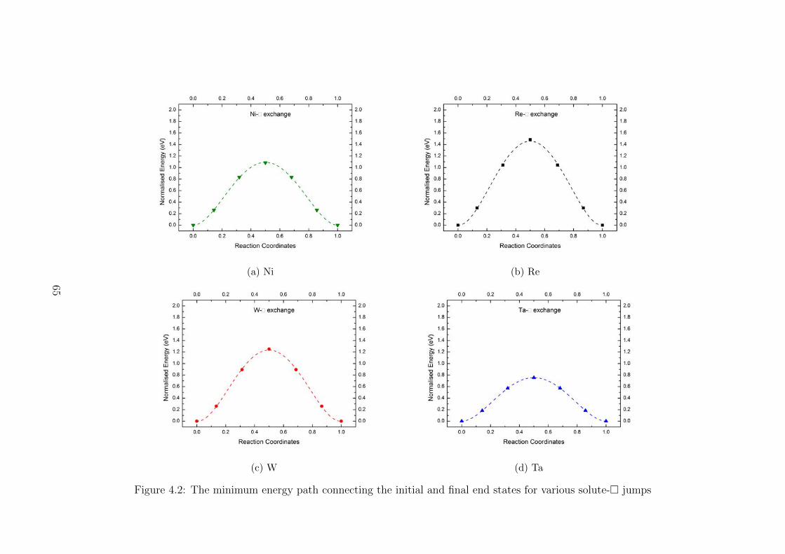
(a) Ni (b) Re

(c) W (d) Ta

Figure 4.2: The minimum energy path connecting the initial and final end states for various solute-� jumps

65

4.1.5 Solute correlation factors

The migration energy barriers for the rotation, dissociation and association of the solute-

� pairs were similarly calculated. Only a single image was used in the NEB calculations,

as described in Section 4.1.4. The explicit calculations have been depicted in Figure 4.3.

The vacancy is located at a 1st nearest neighbour position to the solute atom. Thus, a

vacancy jump from its position to another 1st nearest neighbour position will cause the

solute-� pair rotation. A vacancy jump to a 3rd nearest neighbour position will cause the

solute-� pair dissociation, while a reverse jump would cause the solute-� pair association.

The solute-� pair exchange corresponds to the vacancy exchanging its position with the

solute atom.

It must be noted that there are other possible rotational as well as dissociative jumps

for a solute-� pair, however, the Lidiard’s model [59] only allows a single value for each of

these jumps (see Equation (2.15). The number of possible dissociative jumps to take the

vacancy to a 2nd, 3rd and 4th nearest neighbour positions are 2, 4 and 1 respectively (see

Figure 4.9). Hence, the dissociative jump to a 3rd nearest neighbour position is the most

common one and is used in the calculations here. On the other hand, the solute-� pair

rotation from a 1st nearest neighbour position to another 1st nearest neighbour position

is the only relevant rotational jump in the Lidiard’s model [59]. Section 4.2.1 has a more

elaborate description of the various vacancy jumps around the solute atom.

Table 4.3 shows the calculated values for ∆Erot,i, ∆Edis,i and ∆Eass,i from the present

work. All these values for Re are very similar to the ∆Em,i value of 1.08 eV for the

self-diffusion in Ni suggesting that these jumps are almost independent of the presence of

the Re atom in the neighbourhood. On the other hand, for the case of Ta, these jumps

produce different results, with a value of 1.37 eV for ∆Erot,i, 1.00 eV for ∆Edis,i and only

0.91 eV for ∆Eass,i. The results have been compared to that of the first principles work

of Schuwalow et al [52] and the agreement is very good. However, there was a systematic

decrease of the values by approximately 0.05 eV. This can be attributed to the slightly

different calculation settings used by Schuwalow et al [52], particularly the energy cutoff

66

Figure 4.3: An fcc cell showing a solute atom (black), a vacancy (empty square), the Niatoms (green) and their nearest neighbour relationship to the solute atom and the variousvacancy jumps corresponding to the calculated migration barriers. There are more thanone symmetrically equivalent atoms, but only one case of solute-� pair rotation andsolute-� pair dissociation/association has been shown for clarity.

values.

The solute correlation factors, fi were calculated according to Equation (2.15) and

the values in the temperature range of 1173 K - 1573 K have been shown in Figure 4.4.

The choice of the temperature range was made in order to compare the results for the

calculated diffusion coefficients to previous works in the literature [37, 36], besides covering

the intermediate and high temperature creep regime in Ni-based superalloys. For all

jumps, except for the solute-� exchange, a ν∗i of 2.57 THz was used. It was seen that

the correlation factor varies only slightly for all solute atoms in the temperature range

considered. For the case of Re and W, ∆Erot,i and ∆Edis,i values were found to be much

67

Figure 4.4: The solute correlation factors fi calculated in the temperature range of 1173K to 1573 K.

lower than ∆Em,i, thus yielding a value of fi ≈ 1. Thus, Re and W are expected to

perform a random walk in a dilute alloy of Ni. On the contrary, for the case of Ta, ∆Erot,i

and ∆Edis,i values were much higher than ∆Em,i. This results in a higher Ta-� exchange

frequency and thus a reverse exchange between a Ta atom and a vacancy would be the

most probable event following a successful exchange, which means correlation effects are

strong for Ta diffusion. A fi value of 0.338 was calculated for Ta at 1373 K, in comparison

to a fi value of 0.996 for Re and 0.966 for W.

68

Table 4.3: The calculated terms for self-diffusion and solute diffusion in Ni

Solute ν∗i fi Di0 ∆Ef,i ∆Em,i Qi ∆Erot,i ∆Edis,i ∆Eass,i

(THz) (1373K) (x10-7m2/s) (eV) (eV) (eV) (eV) (eV) (eV)

Niself 2.57 0.781 10.1 1.44 1.08 2.52 - - -4.48 [103] 920 [48],1770 [49], 1.54 [104], 1.73 [105], 1.24 [36] 2.88 [48], 2.955 [49],

1900 [106], 1.58-1.63[107] 1.01 [52] 2.90 [106],920 [108], 400 [109], 1.7[36],1.42 [52] 2.88 [108], 2.77 [109],

3360 [110], 5120 [111] 3.03 [110], 3.08 [111],2.65-2.82 [112]

Re 1.67 0.996 8.37 1.48 1.51 2.99 1.13 1.07 1.088.2 [37], 10.4 [52] 1.46 [52] 2.64 [37], 1.05 [52] 1.00 [52] 1.02 [52]

3.50 [36], 2.91 [52]W 2.36 0.966 11.44 1.46 1.27 2.73 1.20 1.04 1.04

80 [37],11.0 [52], 1.22 [52] 2.74 [37], 3.08 [113], 1.16 [52] 0.98 [52] 0.98 [52]1130 [113], 2200 [114] 3.14 [114],

3.05 [36], 2.66 [52]Ta 2.56 0.338 4.35 1.36 0.77 2.13 1.37 1.00 0.91

219 [37], 15.4 [52] 0.75 [52] 2.60 [37] 1.33 [52] 0.96 [52] 0.86 [52]2.34 [36], 2.28 [52]

69

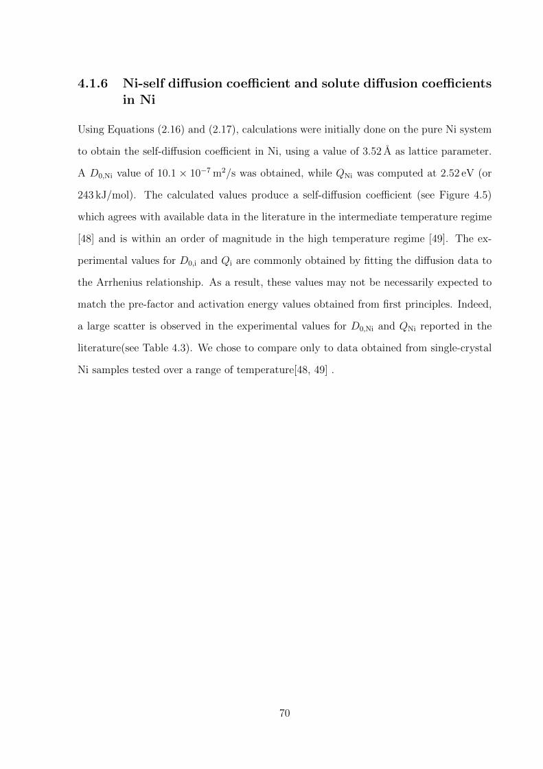
4.1.6 Ni-self diffusion coefficient and solute diffusion coefficientsin Ni

Using Equations (2.16) and (2.17), calculations were initially done on the pure Ni system

to obtain the self-diffusion coefficient in Ni, using a value of 3.52 A as lattice parameter.

A D0,Ni value of 10.1 × 10−7 m2/s was obtained, while QNi was computed at 2.52 eV (or

243 kJ/mol). The calculated values produce a self-diffusion coefficient (see Figure 4.5)

which agrees with available data in the literature in the intermediate temperature regime

[48] and is within an order of magnitude in the high temperature regime [49]. The ex-

perimental values for D0,i and Qi are commonly obtained by fitting the diffusion data to

the Arrhenius relationship. As a result, these values may not be necessarily expected to

match the pre-factor and activation energy values obtained from first principles. Indeed,

a large scatter is observed in the experimental values for D0,Ni and QNi reported in the

literature(see Table 4.3). We chose to compare only to data obtained from single-crystal

Ni samples tested over a range of temperature[48, 49] .

70

0 . 0 0 0 6 0 . 0 0 0 7 0 . 0 0 0 8 0 . 0 0 0 9 0 . 0 0 1 0 0 . 0 0 1 1 0 . 0 0 1 21 E - 2 1

1 E - 2 0

1 E - 1 9

1 E - 1 8

1 E - 1 7

1 E - 1 6

1 E - 1 5

1 E - 1 4

1 E - 1 3

1 E - 1 21 6 6 7 1 4 2 9 1 2 5 0 1 1 1 1 1 0 0 0 9 0 9 8 3 3

T ( K )

D Ni (m2 /s)

1 / T ( K - 1 )

P r e s e n t W o r k B a k k e r M a i e r e t a l

Figure 4.5: The self-diffusion coefficient of Ni calculated from first principles[63] comparedto experimental values (Bakker [49] and Maier et al [48]) .

71

(a) Di for all solutes and DselfNi (b) DRe - comparison

(c) DW - comparison (d) DTa - comparison

Figure 4.6: (a)The solute diffusion coefficients in Ni as a function of temperature. Ni-self diffusion coefficient has been included aswell for comparison. (b)-(d) Comparison of the solute diffusion coefficients to previous works in the literature [37, 36, 52].

72

Calculations were then run for Re, W and Ta as solute atoms in 108-atom supercells.

All the terms in the pre-factors (D0,i) and activation energies (Qi) have been tabulated in

Table 4.3. The resulting diffusion coefficients for Re, W and Ta are shown in Figure 4.6,

and agree with both experimental and theoretical data available in the literature (see

Table 4.3). The diffusivity of Re and W are respectively roughly two orders and one order

of magnitude lower than the diffusivity of the host Ni. In contrast, Ta is expected to diffuse

an order of magnitude faster than Ni. The solute diffusion coefficients calculated from the

present work have also been plotted along with the results from the experimental work of

Karunaratne et al [37] and the first principles work of Janotti et al [36] and Schuwalow

et al [52]. While the results are in excellent agreement with those of Schuwalow et al [52]

for all the solutes in Ni, there is a difference of about an order of magnitude for the case

of Ta when compared to the results of Janotti et al [36]. Similar to the present work,

Schuwalow et al [52] have used the generalized gradient approximation (GGA) to perform

their first principles calculations on 3× 3× 3 supercells, while the results of Janotti et al

[36] were obtained using local density approximation (LDA) on 2× 2× 2 supercells.

A comparison with the experimental work of Karunaratne et al [37] shows a good

match for the case of Ta, but a difference of approximately an order of magnitude for

the cases of W and Re. It must be noted that the reported experimental data was

determined from the interdiffusion coefficients D in these systems. However, experiments

were conducted by these authors over a range of composition in the dilute regime (<

3.5 at.%), and it was observed that D remained independent of composition in all the three

systems in the dilute regime. Assuming the thermodynamic factor in the Darken’s second

equation [43] to be equal to unity, the interdiffusion coefficients D in the dilute regime

should be approximately equal to (within an order of magnitude) the solute diffusion

coefficients Di.

73

4.1.7 Vacancy diffusion coefficients in Ni

Before applying Manning’s random alloy model, its validity for the current system must

be ensured. First, Manning’s model assumes for the binary alloy to be random and

for the solute atoms to have negligible binding energies with vacancies (i.e. vacancy

distribution must also be random). The distribution of Re, W and Ta in Ni has been

the subject of several studies [28, 27, 29], all confirming using a variety of techniques

that the distribution of dilute amounts of these solute atoms in Ni should be expected to

be random at elevated temperatures. The binding energies for solute-� pairs have also

been calculated from first principles (see Figure 4.1). These values are small relative to

the vacancy formation and migration energy, and the distribution of vacancies can be

assumed to be random. Second, Manning’s model assumes that the exchange frequency

of an atom-� pair is only dependent on the atom exchanging places with the vacancy, and

unbiased by the identity of neighbouring atoms. In other words, the migration barriers for

solute-� rotation, dissociation and association should be similar to the migration barrier

of the solvent. This is approximately the case for Re and W (see Table 4.3), but not

the case for Ta, which is not the primary focus of the present study. We can therefore

conclude that, at least for Re and W, Manning’s model for estimating vacancy diffusion

is valid to a first approximation.

Using the values for diffusion coefficients obtained above, we can calculate the vacancy

correlation factor (fv) using in Equation (2.30) as a function of temperature and com-

position for Re and W additions. As discussed in Section 2.1.2, Equation (2.30) breaks

down when the solute atoms diffuse faster than the solvent. Therefore, for Ta, we use

the vacancy correlation factor calculated according to Equation (2.20). The use of Equa-

tion (2.20) for Re and W does not produce substantially different results when compared

to the correlation factors obtained from Equation (2.30). The change of fv with solute

concentration at 1373 K is shown in Figure 4.7. For a pure metal, the vacancy correlation

factor is unity and remains close to unity with small additions (up to 5 at.%) of Re and

W. The addition of a fast-diffusing solute atom, on the other hand, results in a drop in

74

0 . 0 0 0 . 0 1 0 . 0 2 0 . 0 3 0 . 0 4 0 . 0 5

0 . 7 5

0 . 8 0

0 . 8 5

0 . 9 0

0 . 9 5

1 . 0 0

f v

x i

R e W T a

Figure 4.7: Vacancy correlation factors in Ni at 1373 K[63]

fv due to the fact that reverse solute-� exchanges are more likely than Ni-� exchanges.

Finally, the vacancy diffusion coefficient in a dilute binary alloy, Dv, can be estimated.

The results for 1373 K in binary Ni alloys with up to 5 at.% Re, W and Ta are shown

in Figure 4.8. Also in this case, Re and W are seen to decrease the vacancy diffusion

coefficient, albeit the effect is small. The addition of 5 at.% Re and W results in a

reduction of vacancy diffusion coefficient of less than 10% when compared to vacancy

diffusion in pure Ni. The addition of Ta, as expected, increases the vacancy diffusion

rate. The lower vacancy correlation factor in the presence of Ta additions does not negate

the effects of the higher Ta-� exchange frequency on the overall vacancy diffusion rate.

75

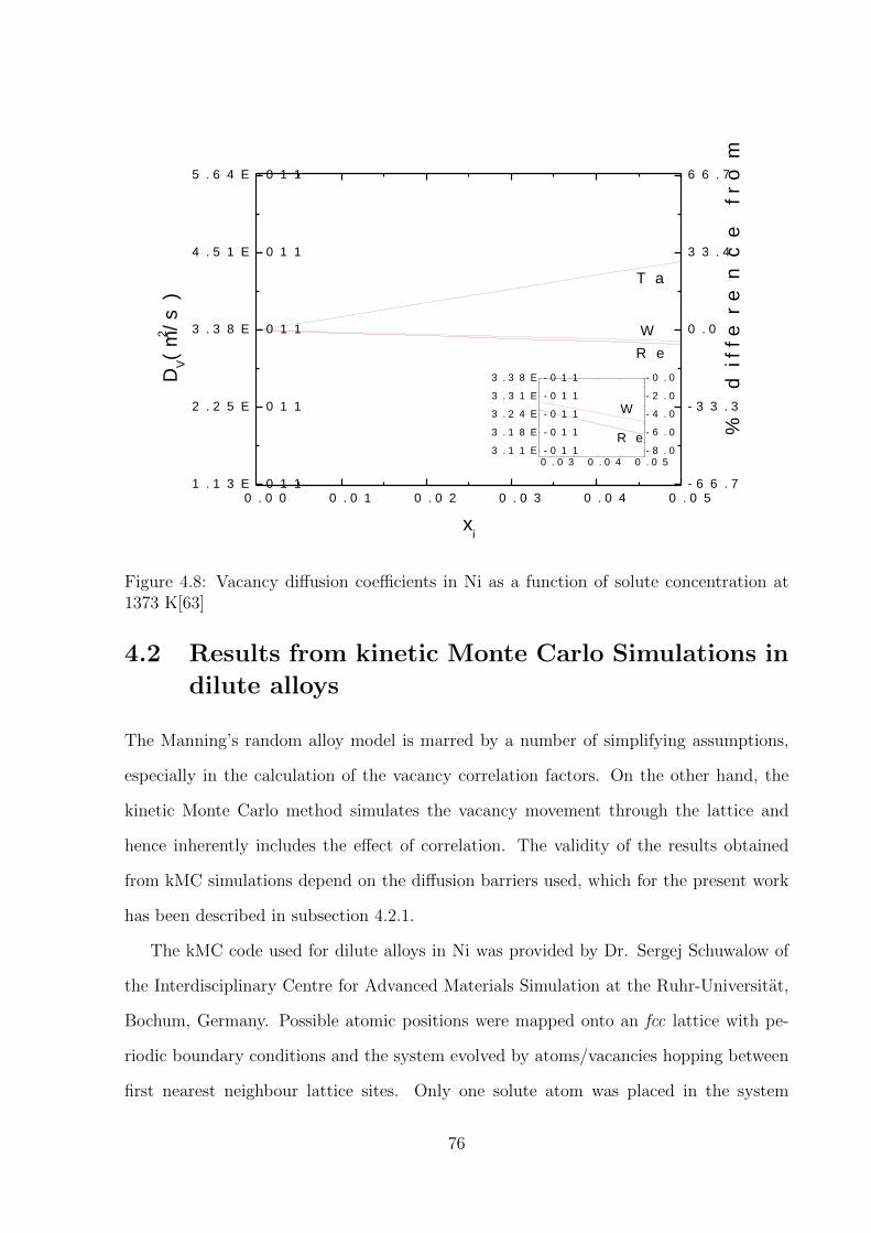
0 . 0 0 0 . 0 1 0 . 0 2 0 . 0 3 0 . 0 4 0 . 0 51 . 1 3 E - 0 1 1

2 . 2 5 E - 0 1 1

3 . 3 8 E - 0 1 1

4 . 5 1 E - 0 1 1

5 . 6 4 E - 0 1 1

- 6 6 . 7

- 3 3 . 3

0 . 0

3 3 . 4

6 6 . 7

% di

fferen

ce fro

m pu

re Ni

D V(m2 /s)

x i

R eW

T a

0 . 0 3 0 . 0 4 0 . 0 53 . 1 1 E - 0 1 13 . 1 8 E - 0 1 13 . 2 4 E - 0 1 13 . 3 1 E - 0 1 13 . 3 8 E - 0 1 1

- 8 . 0- 6 . 0- 4 . 0- 2 . 0- 0 . 0

WR e

Figure 4.8: Vacancy diffusion coefficients in Ni as a function of solute concentration at1373 K[63]

4.2 Results from kinetic Monte Carlo Simulations in

dilute alloys

The Manning’s random alloy model is marred by a number of simplifying assumptions,

especially in the calculation of the vacancy correlation factors. On the other hand, the

kinetic Monte Carlo method simulates the vacancy movement through the lattice and

hence inherently includes the effect of correlation. The validity of the results obtained

from kMC simulations depend on the diffusion barriers used, which for the present work

has been described in subsection 4.2.1.

The kMC code used for dilute alloys in Ni was provided by Dr. Sergej Schuwalow of

the Interdisciplinary Centre for Advanced Materials Simulation at the Ruhr-Universitat,

Bochum, Germany. Possible atomic positions were mapped onto an fcc lattice with pe-

riodic boundary conditions and the system evolved by atoms/vacancies hopping between

first nearest neighbour lattice sites. Only one solute atom was placed in the system

76

to model the dilute alloys. Also, only one vacancy was placed in the system to avoid

vacancy-vacancy interactions. This is a good approximation as the vacancy concentration

in metallic alloys like Ni tend to be small even at high temperatures.

4.2.1 Migration energy barriers for extended vacancy jumps

A number of migration barriers have been included to model the system to a greater

accuracy. Under dilute approximation, only one solute atom has been included in the

system, hence migration barriers for a solute-� exchange in the presence of another solute

atom has not been considered. We expect the results to be valid in the dilute limits of

less than 1 at. %.

All the vacancy jumps up to the 4th nearest neighbour distance to the solute atom

have been considered. These have been depicted in Figure 4.9 and consist of a solute-�

exchange (red dashed line), three instances of solute-� pair dissociation/association (blue

dashed lines), one solute-� pair rotation and five other extended rotation jumps within

the fourth neighbour shell of the solute atom (green dashed lines)[52]. Jumps beyond

the 4th nearest neighbour shell of the solute atom were unaffected by the presence of the

solute atom, and hence the ∆Em,Ni value was used for these jumps. The activation energy

barriers have been calculated from first principles using 3×3×3 supercells and the results

tabulated in Table 4.4. As an example, jump 2→3 means a vacancy jumping from a 2nd

nearest neighbour position of the solute atom to a 3rd nearest neighbour position of the

solute atom.

A value of 2.57 THz was used as the effective frequency ν∗ for all jumps. The kMC

simulations were performed as described in 2.2. All the atoms and the vacancy were

tracked over time to calculate the diffusion coefficients.

77

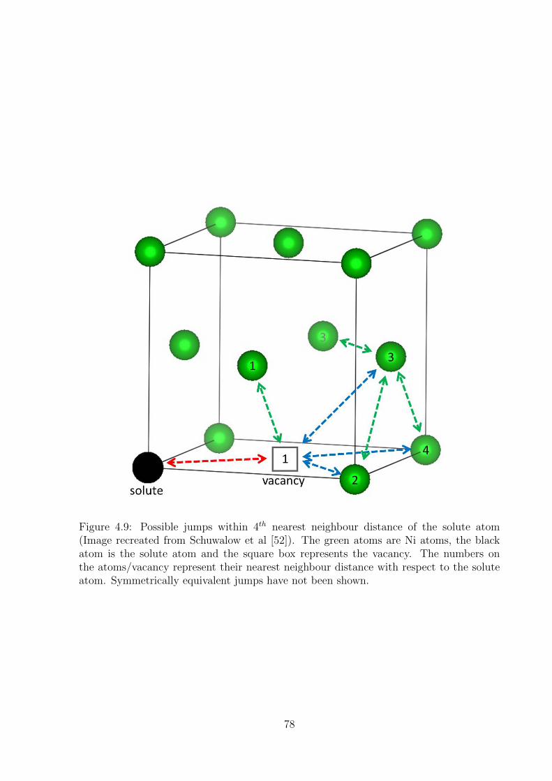
Figure 4.9: Possible jumps within 4th nearest neighbour distance of the solute atom(Image recreated from Schuwalow et al [52]). The green atoms are Ni atoms, the blackatom is the solute atom and the square box represents the vacancy. The numbers onthe atoms/vacancy represent their nearest neighbour distance with respect to the soluteatom. Symmetrically equivalent jumps have not been shown.

78

Table 4.4: The migration barriers for solute-� exchange and solute-� extended rotation, dissociation and association used in thekinetic Monte Carlo simulations for dilute alloys

Solute∆Em,i(eV) ∆Erot,i (eV) ∆Edis,i (eV) ∆Eass,i (eV)

0→1 1→1 2→3 3→2 3→3 3→4 4→3 1→2 1→3 1→4 2→1 3→1 4→1

Niself 1.08 - - - - - - - - - - - -

Re 1.51 1.13 1.12 1.04 1.07 1.07 1.15 0.95 1.07 1.06 1.05 1.08 1.14

W 1.27 1.20 1.11 1.08 1.06 1.07 1.16 0.97 1.04 1.05 1.00 1.04 1.13

Ta 0.77 1.37 1.10 1.12 1.05 1.08 1.18 1.01 1.00 1.02 0.89 0.91 1.02

79

4.2.2 Ni-self diffusion coefficient and solute diffusion coefficientsin Ni

The results for the Ni-self diffusion coefficient and solute diffusion coefficients in Ni for

the temperature range 1173 K to 1573 K have been shown in Figure 4.10. These kMC

simulations were run on 15×15×15 supercells, with 13500 lattice sites containing 1 solute

atom and 1 vacancy. The kMC trajectory was divided into segments of 2000 jumps,

and the diffusion coefficients obtained from kMC simulations were averaged over these

segments. The results converged after approximately 107 jumps. Five different trials were

run for each temperature and the arithmetic means of the diffusion coefficients from those

trials were reported. The vacancy concentration of the simulation cell was 0.0074 at.% and

hence the obtained diffusion coefficients were corrected as described in Equation (2.34)

with the actual vacancy concentration in Ni at the temperature T given according to

Equation (2.7). A ∆Ef,i value of 1.44 eV was used in all the cases.

Figure 4.10 also shows a comparison of the kMC results (symbols) to those previously

obtained by Lidiard’s model (lines). The diffusion trend was the same with Ta being

the fastest diffuser, and Re being the slowest. The results for Ni and W almost overlap,

while the results for Re and Ta are very close. Some of the differences can be attributed

to the fact that the Lidiard’s model (Equation 2.15) assumes a single value each for

the ∆Erot,i and ∆Edis,i (or ∆Eass,i). However, the results in Table 4.4 show that there

are considerable variations depending on which nearest neighbour position the vacancy is

jumping to. For example, ∆Edis,Re value for 1→2 dissociation is only 0.95 eV, while that

for a 1→3 dissociation is 1.07 eV.

Since a number of diffusion barriers were considered in the kMC simulations, a de-

composition of the solute diffusion coefficient Di into the diffusion pre-factor, Di0 and

activation energy, Qi terms could be non-trivial. These values were extracted from the

kMC data in Figure 4.10 and have been tabulated in Table 4.5. A comparison to the data

obtained from Lidiard’s model, however shows a very good match for all the solutes. This

shows that the application of the Lidiard’s model in the investigated systems produces

80

Table 4.5: The Di0 and Qi terms extracted from the kMC data for self-diffusion and solute

diffusion in Ni compared to the previously calculated results from Lidiard’s model (LM)in the present work

Solute Method Di0 Qi

(x10-7m2/s) (eV)

Niself kMC 11.33 2.53LM 10.1 2.52

Re kMC 12.77 2.99LM 8.37 2.99

W kMC 15.18 2.74LM 11.44 2.73

Ta kMC 18.44 2.35LM 4.35 2.13

results of the same level of accuracy as the kMC simulations. The results were also in

excellent agreement to those obtained by Schuwalow et al [52] from their kMC studies

(see Table 4.3).

However, a small deviation was found in the case of Ta when compared to the results

from Lidiard’s model. This can be explained as follows. The solute correlation factor, fi

was included in the diffusion pre-factor term Di0 as shown in Equation (2.16), however

fi is expected to affect the exponential term, Qi as well, given its dependence on the

various diffusion barriers. For Re and W, the solute correlation factor, fi was found to

be nearly unity for the temperature range considered, while for the self-diffusion of Ni,

the correlation factor is a constant. For Ta, however, the fi value varied between 0.3

to 0.4 in the temperature range considered (see Figure 4.4). Thus, a lower value of Di0

was obtained for Ta from Lidiard’s model. However, as seen from the kMC results, the

contributions of fi for the case of Ta have mostly entered the Qi term and hence we have

a higher Qi value for Ta. It must be noted that a higher value of Qi has the same effect

on the solute diffusion coefficient as a lower value of Di0.

81

Figure 4.10: The self-diffusion coefficient in Ni and solute diffusion coefficients in Ni as afunction of temperature. The symbols represent the results from kMC simulations, whilethe lines represent the results calculated from Lidiard’s model

82

4.2.3 Vacancy diffusion coefficients in Ni

Similarly, the vacancy diffusion coefficients were also calculated in pure Ni and binary

alloys of Ni under dilute limits. The solute concentration was varied by changing the size

of the supercells used in the kMC simulation. The smallest kMC cell size was 3×3×3,

limiting the maximum solute concentration to about 0.9 at.%. Other cell sizes used were

3×3×4, 3×4×4, 4×4×4, 5×5×5, 6×6×6 and 15×15×15 yielding solute concentrations

of 0.7 at.%, 0.5 at.%, 0.4 at.%, 0.2 at.%, 0.1 at.% and 0.0074 at.% respectively. Five

kMC simulation runs were performed at 1373 K and the mean Dv was calculated. The

results have been plotted in Figure 4.11. A Dv value of 3.46 × 10−11 m2/s was obtained

in pure Ni at 1373 K which matches exactly with the value predicted from analytical

formulations (DNiv is simply equal to a2ΓNi). When compared to the results on Dv from

Manning’s model (see Figure 4.8), we can see that both predict that Dv for Re and W

almost overlap, however the magnitude of the decrease in Dv is much greater from the

kMC simulations. If we extrapolate the kMC results, a 5 at.% addition of Re or W should

reduce the Dv by almost 30%. Similarly, a 5 at.% addition of Ta is expected to increase

the Dv by about 20%.

4.2.4 Discussion

The analytical model for vacancy diffusion developed by Manning [64] indicated that small

additions of slow-diffusing atoms in a host fcc lattice do not reduce the diffusion rate of

vacancies substantially. In the case of slow diffusing solute atoms, the correlation factor

for vacancy diffusion from Manning’s formulation remains close to unity, and the decrease

in Γv is minor. Manning’s model suggests that vacancies would rarely have to exchange

with the slow-diffusing solute atom, and even in the case the solute atoms were to be

absolutely immobile due to a very high activation energy barrier for solute-� exchange,

the resulting effect would only be as big as the percentage of solute content.

However, Manning’s model was based on a number of simplifying assumptions and,

83

Figure 4.11: Vacancy diffusion coefficients in Ni as a function of solute concentration at1373 K as calculated from the kMC simulations in dilute alloys

to get a more accurate description, kMC simulations were run to model the binary alloys

in Ni. In the dilute regime, different migration barriers around a solute atom up to

the 4th nearest neighbour distance were considered. Results from kMC simulations on

dilute alloys showed a much greater impact of the solute atoms on the vacancy diffusion

coefficients.

It was noteworthy that both the Manning’s model as well as kMC simulations in

the dilute regime predicted additions of Re and W to have the same effect on vacancy

diffusion. While Re diffusion in Ni is almost an order of magnitude slower than W, it is

more important to understand how they affect the Ni jump barriers in their vicinity, as the

vacancy is more likely to exchange with Ni atoms. Indeed, looking at the extended jump

barriers considered for the kMC simulations (see Table 4.4), it is clear that Re and W

both have similar effects on the Ni jump barriers. In the seminal work of Giamei et al [11]

on Re-effect, the observed improvements in creep lives of their model alloy was attained

84

by substituting W with Re. Thus, one would expect significantly different effects of these

two solutes on Dv in Ni. However, it must also be noted that unlike W, Re partitions

strongly to the γ phase, and thus the observed difference in creep strengthening could be

simply a result of its higher concentration in the γ phase. It is therefore important to

investigate how non-dilute alloys of Re in Ni affect the Dv. In non-dilute alloys, the solute

- solute interactions will have to be taken into account to properly describe the diffusion

processes.

85

CHAPTER 5

BINARY CLUSTER EXPANSION INNICKEL-RHENIUM

The CASM (Cluster-Assisted Statistical Mechanics) code developed by Anton Van der

Ven and coworkers [81, 82] was used for the cluster expansion of the configurational energy

in the Ni-Re binary. A primitive fcc cell with configurational degree of freedom was given

as the input to generate Ni-Re configurations in the entire binary composition space for

maximum 10 atom supercells. 87 fcc supercells with a total of 2146 symmetrically distinct

configurations were generated. Among these 2146 configurations, all possible configura-

tions for supercells containing up to 4 atoms were selected while for bigger supercells,

the configurations with Re concentration ≤ 20 at.% were selected. This was done to bias

the cluster expansion to predict energies more accurately in the Ni-rich region. Thus, a

total of 144 configurations were selected and their first principles energy was calculated.

The cell volume, shape and all the internal degrees of freedom were relaxed. All calcu-

lations were spin-polarized. The electronic self-consistent loops were stopped when the

total energy converged to within 10−6 eV and ionic positions were relaxed until all forces

fell below 10−2 eV/A. A 37 × 37 × 37 k-point mesh was used for the primitive fcc cell.

This has the same k-spacing in the reciprocal lattice [100] as a 5× 5× 5 k-point mesh for

a 108 atom fcc supercell which has been used for the calculations in the previous chapter.

To maintain the same k-spacing, the k-mesh was automatically adjusted for the different

configurations depending on their lattice vectors. Other details for the calculations were

86

same as given in subsection 3.3. On re-running the code, the formation energy per atom

Eform of these 144 configurations were calculated according to the equation,

Eform =ENixRey − xENi − yERe

(x+ y)(5.1)

where ENixRey is the energy of the configuration NixRey, x and y being the number of Ni

and Re atoms respectively. ENi and ERe are the energy of pure Ni and pure Re (calculated

from first principles) used as reference states (see Table 5.2). Since all the configurations

used in the present work were fcc, the energy for fcc Re was used as the reference. It

must be noted that pure Re exhibits an hcp structure, however, in the Ni-rich regions,

Re is expected to be present in an fcc solution of Ni. The formation energies of these

configurations are shown in Figure 5.1. Amongst all the 144 configurations considered

in Figure 5.1, the stoichiometric compound Ni4Re at 20 at.% Re with a D1a structure

was the lowest energy configuration with a formation energy of -0.073 eV. 101 of these

configurations were used to fit the ECIs for the cluster expansion. Configurations with

a formation energy greater than 0.03 eV were discarded as their formation is less likely

energetically. Also, configurations towards the Ni-rich side were preferred. Specifically,

the configurations with a Re concentration greater than 33 at.% were discarded. This

was partly because the concentration of Re in the γ phase even in the third generation of

Ni-based superalloys never goes beyond 10 at.% [115]. It is unlikely that even the local

composition in the γ phase due to statistical fluctuations would go beyond 33 at.%. The

calculation of the ECIs will be discussed in detail in the next section.

There have been previous investigations on the binary Ni-Re system using cluster

expansion [32, 31]. Maisel et al [32] used the UNCLE package [116] to predict formation

energies of 213,061 symmetrically inequivalent fcc structures of up to 20 atoms with 0 -

33 at.% Re by fitting their ECIs to a first principles database of 155 of those structures.

The calculations were spin-polarized. Apart from pure Ni, D1a-Ni4Re with a formation

energy of -0.058 eV was predicted to be a dominant ground-state structure, with a sizeable

gap in its energy compared to all the other configurations used in their cluster expansion.

87

However, the calculated ECIs have not been reported. Monte Carlo simulations suggested

the precipitation of D1a-Ni4Re in a lattice of Ni at low temperatures and remnant short

range ordering at high temperatures.

He et al [31] have calculated two types of ECIs. The first were called ‘fully renormalized

interactions’ and had a formulation similar to binding energies, while the other ECIs

were dependent on composition, temperature and magnetism. The ECIs generated in the

present work are composition independent and hence a comparison was again not possible.

Formation energies > 0 were calculated for random alloys of Re in Ni in the dilute range

with spin-polarized calculations indicating phase separation. However, with non spin-

polarized calculations, formation energies < 0 were calculated indicating ordering in the

Ni-Re system. They calculated the formation energy of D1a-Ni4Re as -0.062 eV using

spin-polarized calculations and -0.106 eV using non spin-polarized calculations. It must be

noted that fcc Ni and hcp Re were used as the reference states in their work. Other ordered

compounds with compositions Ni15Re and Ni8Re were also found to be stable using non

spin-polarized calculations, and hence a simple separation into fcc Ni and D1a-Ni4Re

would not be expected. It can be argued that the non-magnetic state is representative

of the high temperature behaviour in these alloys, given that Ni loses its ferromagnetic

property above its Curie temperature. However, as mentioned in subsection 1.3.3, a

complete consideration should also include the thermal magnetic excitations [31]. Thus it

remains inconclusive whether spin-polarized or non spin-polarized calculations represent

the Ni-Re system better.

Levy et al [117] used high-throughput first principles calculations to predict the for-

mation of stable ordered compounds in Ni-Re alloys amongst other binary alloys of Re.

Apart from D1a-Ni4Re, whose formation energy was calculated as -0.064 eV they also

found the stable D019-NiRe3 structure with a formation energy of -0.115 eV using spin-

polarized calculations. However, D019 is an hcp based structure in the Re-rich side of the

Ni-Re binary, and hence could not be accounted in the cluster expansion described in the

present work.

88

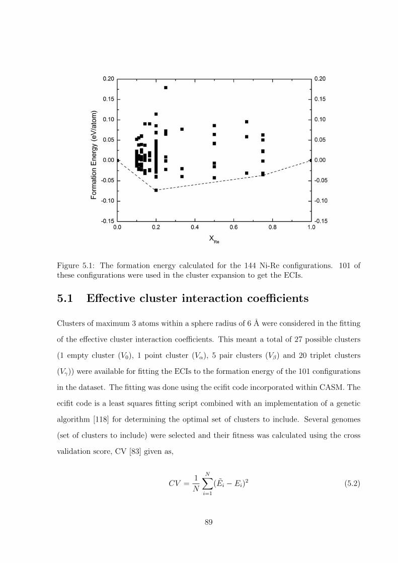
Figure 5.1: The formation energy calculated for the 144 Ni-Re configurations. 101 ofthese configurations were used in the cluster expansion to get the ECIs.

5.1 Effective cluster interaction coefficients

Clusters of maximum 3 atoms within a sphere radius of 6 A were considered in the fitting

of the effective cluster interaction coefficients. This meant a total of 27 possible clusters

(1 empty cluster (V0), 1 point cluster (Vα), 5 pair clusters (Vβ) and 20 triplet clusters

(Vγ)) were available for fitting the ECIs to the formation energy of the 101 configurations

in the dataset. The fitting was done using the ecifit code incorporated within CASM. The

ecifit code is a least squares fitting script combined with an implementation of a genetic

algorithm [118] for determining the optimal set of clusters to include. Several genomes

(set of clusters to include) were selected and their fitness was calculated using the cross

validation score, CV [83] given as,

CV =1

N

N∑i=1

(Ei − Ei)2 (5.2)

89

Figure 5.2: ECI/multiplicity for pair and triplet clusters

where Ei is the formation energy of configuration i, and Ei is the energy predicted

for configuration i by the least squares fit obtained with configuration i excluded. N is

the number of configurations in the dataset. Genetic algorithm is inspired by the rule of

evolution. The low performing genomes are culled and the high performing genomes are

mated to produce new generation of genomes.

The ECIs were optimised after about 20 such generations. Sufficient accuracy was

obtained when using a total of 15 clusters. The root mean square error between first-

principles energies and cluster expanded energies for all 101 structures used in the fit was

5.7 meV per atom and the CV score was 7.3 meV per atom. This is a good fit considering

the fact that an rms error value of 5.6 meV per atom was obtained by Van der Ven et al

[84] using their ECIs calculated for Al-Li alloys.

90

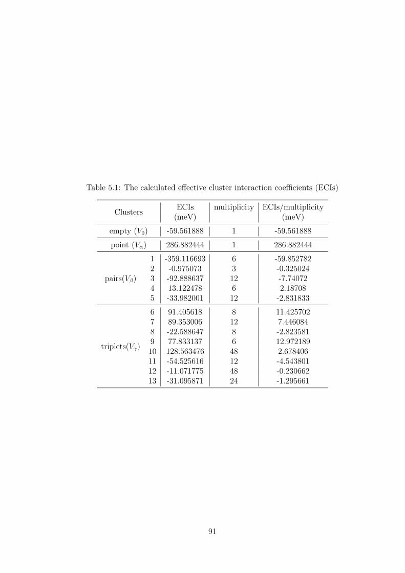
Table 5.1: The calculated effective cluster interaction coefficients (ECIs)

ClustersECIs multiplicity ECIs/multiplicity

(meV) (meV)

empty (V0) -59.561888 1 -59.561888

point (Vα) 286.882444 1 286.882444

pairs(Vβ)

1 -359.116693 6 -59.8527822 -0.975073 3 -0.3250243 -92.888637 12 -7.740724 13.122478 6 2.187085 -33.982001 12 -2.831833

triplets(Vγ)

6 91.405618 8 11.4257027 89.353006 12 7.4460848 -22.588647 8 -2.8235819 77.833137 6 12.97218910 128.563476 48 2.67840611 -54.525616 12 -4.54380112 -11.071775 48 -0.23066213 -31.095871 24 -1.295661

91

(a) pair clusters 1 to 5 (b) triplet clusters 6 to 8

(c) triplet clusters 9 to 11 (d) triplet clusters 12 and 13

Figure 5.3: The pair and triplet clusters used in the ECI fitting

92

Table 5.1 shows the fitted ECIs for the Ni-Re case. Five pair clusters (Vβ) include

the 1st five nearest neighbour pairs. Eight triplet clusters (Vγ) have also been included.

These pair and triplet clusters have been numbered 1 to 13 and Figure 5.3 represents

these clusters. The empty cluster (V0) is just a constant term used in the fitting while

the point cluster (Vα) is the single atom cluster. Table 5.1 also shows the multiplicity of

these clusters. For example, the pair cluster number 1 has a multiplicity of 6, meaning

there are 6 symmetrically equivalent clusters in different orientations. This is expected as

an atom in an fcc lattice is paired to twelve 1st nearest neighbours, and each of these pairs

is shared by 2 atoms. Hence, the multiplicity is 6. The ECIs/multiplicity (see Figure 5.2)

have also been calculated as this is more suitable in our kinetic Monte Carlo code to

model the energy of the Ni-Re alloys. As described earlier, an occupation variable (σi)

value of +1 represents a Ni atom, while -1 represents a Re atom. It must be noted that

the CASM code cluster expands the formation energy and not the total configurational

energy. One can calculate the formation energy first from the obtained ECIs, and then

the configurational energy can be deduced by rearranging the Equation (5.1).

The pair cluster (Vβ) number 1 has a significantly larger value compared to the rest.

A large negative value also indicates that the energy predicted for a Ni-Re system will

lower significantly when there are two Ni atoms or two Re atoms as 1st nearest neighbour

pairs. When a Ni atom is surrounded by Re atoms in its 1st nearest neighbour shell, or

vice-versa, there is an increase in the total energy. All other pair clusters except number

4 have negative values. Thus most of the other Re-Re pairs also lower the overall energy

of the system, albeit to a lesser degree. This should mean that two Re atoms would prefer

to sit next to one another in a 1st nearest neighbour position compared to any other

configuration. On the other hand, the triplet cluster (Vγ) number 6 has a positive value.

Thus, if there is a Re 1st nearest neighbour triplet, the occupation vector (~σ) becomes -1,

and the energy of the system is lowered again. However, if the cluster consists of a pair

of Re atoms, and a single Ni atom, then (~σ) becomes +1, and the energy of the system

increases. Thus, strictly speaking, the ECIs cannot be evaluated separately, as the value

93

Table 5.2: The first principles energy and energy predicted from cluster expansion ofNi-Re by the CASM code for pure Ni and pure Re

Reference state FP energy (eV) CE predicted energy (eV)

Ni -5.46864 -5.4473Re (fcc) -12.3403 -13.4285

of one depends on the others.

Table 5.2 presents a comparison of the first principles energy and the energy predicted

from cluster expansion using the above ECIs for pure Ni and pure Re (fcc). One can

see that the match is very good for Ni, while there is a deviation of about 1 eV in

the case of Re. This can be explained as only Ni-rich configurations were used to fit

the ECIs. Nevertheless, we expect accurate prediction of the configurational energies in

the composition range of interest (< 10 at. % Re). It must be clarified that the first

principles energies for pure Ni and Re have been used to calculate the formation energies

in Equation (5.1).

The generated ECIs in the present work were used to calculate the Re-Re pair binding

energies as a function of distance and were compared to the binding energies calculated

directly from first principles with spin-polarization. This has been shown in Figure 5.4.

The results differ by a magnitude of about 0.2 eV, but the predicted trend is very similar

up to 5th nearest neighbour position. Considering that the maximum separation of atoms

in the clusters included in the fit was 5th nearest neighbours, this is expected. The

match improves from Re nearest neighbour pairs to triplets to quadruplets, as shown in

Table 5.3. This means that the generated ECIs are expected to predict the energies for

higher concentration of Re in Ni with a higher accuracy.

Also shown are the results of Mottura et al [29] for non-spin polarized calculations.

It is noteworthy how the binding energy becomes more repulsive with the increase in

the number of Re atoms in the cluster, which contradicts the results from spin-polarized

calculations. This effect was also observed previously by He et al [31]. This means that

the inclusion of magnetism in the calculations can have dramatic consequences to the

94

Figure 5.4: Comparison of the Re-Re binding energies from first principles, predictionsfrom cluster expansion and non-spin polarized results from Mottura et al [29]

phase equilibrium in Ni-Re alloys. While the work of Mottura et al [29] suggests that

Re should be distributed randomly in a solution with Ni, the present work suggests that

a phase separation should be the likely scenario. The results from the cluster expansion

performed by Maisel et al [32] including spin-polarization in their calculations however

predict ordering in the Ni-Re system with the precipitation of D1a-Ni4Re.

Table 5.3: Comparison of the binding energies for different Re clusters from first principles,predictions from cluster expansion and non-spin polarized results from Mottura et al [29]

Re cluster FP energy (eV) CE predicted energy (eV) Mottura et al [29]

pair 0.186 -0.008 -0.425triplet 0.306 0.066 -1

quadruplet 0.379 0.315 -1.65

95

Figure 5.5: The clusters used for expansion of the effective vacancy formation energy(adopted from Van der Ven et al [84])

5.2 Effective vacancy formation energy

The presence of vacancies was accounted by the effective vacancy formation energy as

described in subsection 2.3.1. A local cluster expansion of the EVFE was done around

one vacancy. Unlike the binary cluster expansion, where supercells of maximum 10 atoms

were used, here first principles energy calculations were run on 3×3×3 supercells to avoid

the vacancy-vacancy interaction across the periodic images. 26 different configurations

were used and three calculations were performed on each of them, one with a vacancy at

a lattice site (Evi (�σ)) and two others with a Ni (ENi

i (�σ)) and a Re (ERei (�σ)) atom each

replacing that site. Thus 78 different calculations were performed in total. Configurations

with upto 36 Re atoms (33 at.%) were considered in the calculations. For some of the

non-dilute compositions considered, the ionic relaxation was terminated when the forces

fell below 0.02 eV/A. Also, a 4×4×4 k-mesh was used for these calculations.

The selection of clusters and the fitting of the corresponding ECIs for binary cluster

expansion of the configurational energy in Ni-Re was performed using a genetic algorithm

as incorporated in the CASM code. However, the option of local cluster expansion for

the prediction of EVFE was not available with CASM. Hence, in this case, clusters as

shown in Figure 5.5 were adopted from the work of Van der Ven et al [84]. Four point

clusters up to the 4th nearest neighbour distance, and the 1st nearest neighbour pair

and triplet clusters around a vacancy were considered. LECIs corresponding to these

clusters were fit using multiple regression and the results are shown in Figure 5.6 and also

96

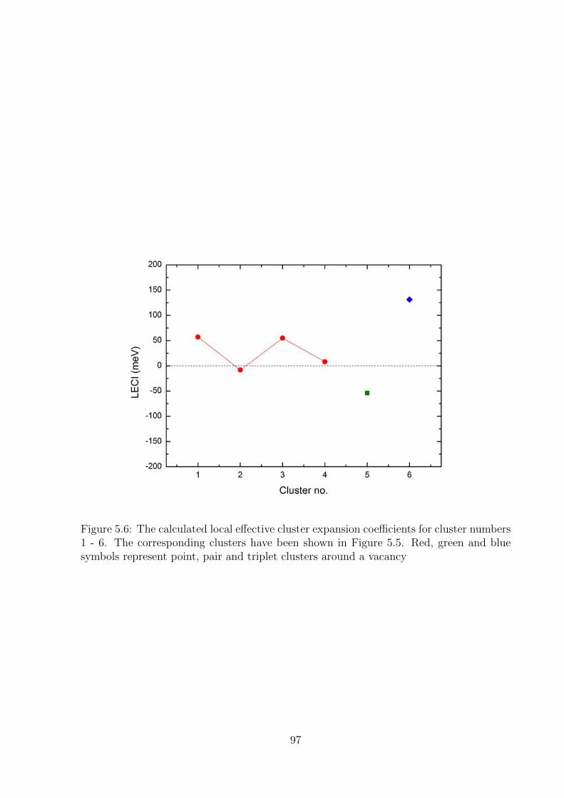
Figure 5.6: The calculated local effective cluster expansion coefficients for cluster numbers1 - 6. The corresponding clusters have been shown in Figure 5.5. Red, green and bluesymbols represent point, pair and triplet clusters around a vacancy

97

Table 5.4: The calculated local effective cluster expansion coefficients (LECIs)

Cluster No. LECIs(meV)

1 57.142 -8.233 54.884 8.06

5 -54.13

6 131.21

tabulated in Table 5.4. LECIs representing different clusters have been given different

colours in Figure 5.6, with red, green and blue symbols representing point, pair and

triplet clusters around a vacancy respectively. It must be noted that the treatment of

the cluster expansion is slightly different here, and instead of considering the occupation

variables for all the atoms around a vacancy, the EVFE was fit to the number of Re

atoms, Re pairs and Re triplets around a vacancy. The constant term was set as 10.2413

eV, which was the EVFE in pure Ni. A root mean square error of 0.083 eV was obtained.

This is clearly higher when compared to the rms error for the binary CE. In order to

assess the quality of the obtained fit, the calculated LECIs have been used to predict

the Re-� binding energies as shown in Figure 5.7. The predicted values match well with

the Re-� binding energies calculated directly from first principles. A discrepancy in the

trend was observed after the 4th nearest neighbour distance. This was expected since

interactions only upto 4th nearest neighbours were included in the EVFE fit. However,

given the reproducibilty of the binding energies otherwise, we expect good results for the

EVFE predictions.

5.3 Kinetically resolved activation energy barriers

The kinetically resolved activation barriers were calculated for a number of vacancy path-

ways with different atomic environments. On top of the barriers considered for the dilute

98

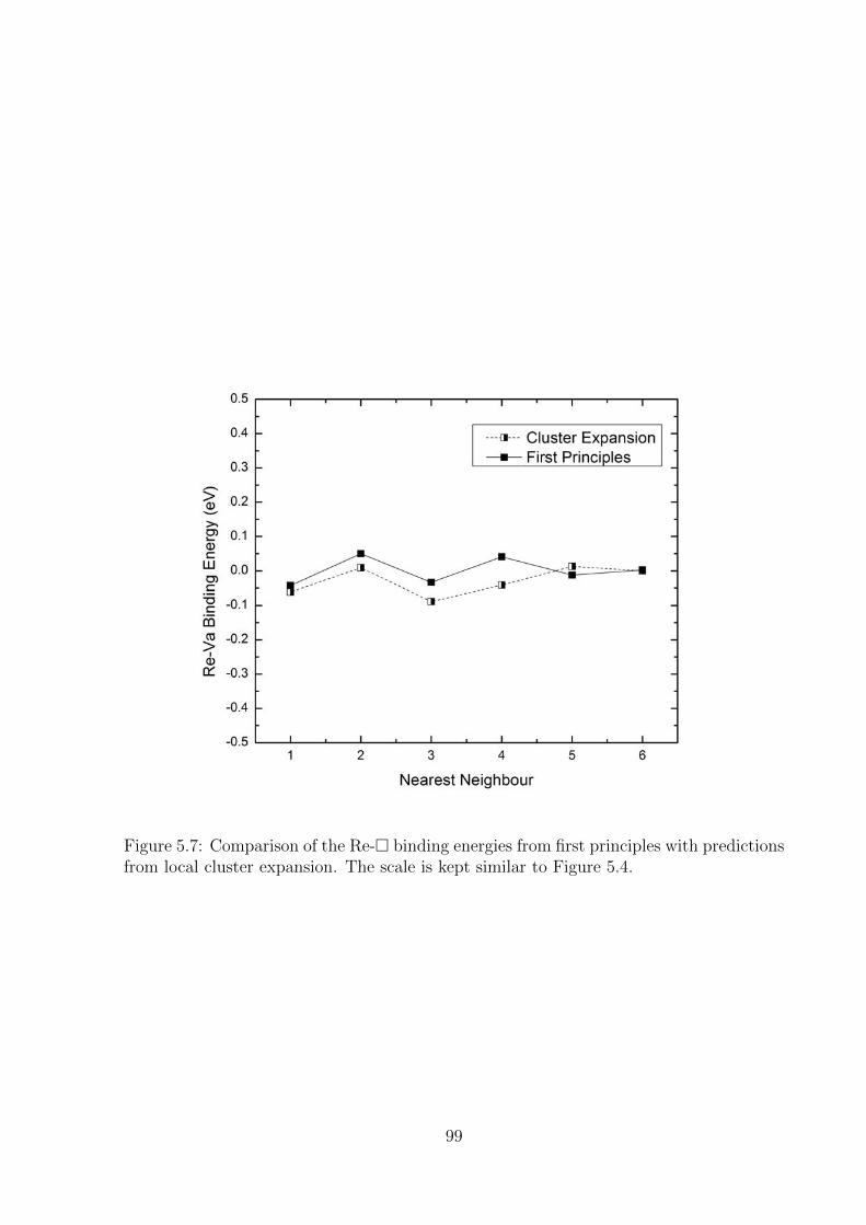
Figure 5.7: Comparison of the Re-� binding energies from first principles with predictionsfrom local cluster expansion. The scale is kept similar to Figure 5.4.

99

Table 5.5: KRAs calculated for the various Re jumps

Type of Re jump ∆Em(eV) ∆EKRA (eV)

S+R 1.604 1.604S+D 1.463 1.512S+A 1.560 1.512

alloys of Ni-Re in Section 4.2.1, other barriers based on the fourteen-frequency model [51]

were considered. These have been illustrated in Figures 5.8, 5.9 and 5.10 (S stands for

vacancy-solute exchange, while R, D and A stand for vacancy-solute pair rotation, dis-

sociation, and association respectively). The barriers were calculated using the climbing

image nudged elastic band method for the forward and the reverse jumps and the KRA

was deduced from the two (see Tables 5.5 and 5.6).

Re jumps

Figure 5.8: Configurations used for Re jumps

100

Ni jumps

When the Re atoms are paired

Figure 5.9: Configurations used for Ni jumps when the Re atoms are paired

101

When the Re atoms are unpaired

Figure 5.10: Configurations used for Ni jumps when the Re atoms are unpaired

102

Table 5.6: KRAs calculated for the various Ni jumps

Type of Ni jump ∆Em(eV) ∆EKRA (eV)

R+R 1.287 1.287

paired D+D 1.046 1.067

Re A+A 1.088 1.067

atoms R+D 1.189 1.169

R+A 1.150 1.169

A+D 1.067 1.067

R+R 1.361 1.361

unpaired D+D 1.069 1.105

Re atoms A+A 1.141 1.105

R+D 1.112 1.147

R+A 1.181 1.147

KRAs were also described using a local cluster expansion according to Equation (2.39).

From definition, KRAs are independent of the direction of the jumping atom and they

represent the saddle point energy normalised to the arithmetic mean of the energies of the

two end points. Thus the occupation variables defined for the local cluster expansion for

KRAs should be centred about the saddle point, in contrast to the local cluster expansion

of EVFE, where the occupation variables were defined in relation to their distance from

the vacancy. However, the saddle point does not overlap on a lattice site and lies ap-

proximately halfway between the hopping atom and the vacancy. Thus, the set of lattice

positions at a certain distance from the hopping atom, and the set of lattice positions at

the same distance from the vacancy are considered equivalent and are clubbed together.

For example, the lattice positions which are 1st nearest neighbours to either the hopping

atom or the vacancy are considered equivalent.

For simplification, the KECIs in the present work were fit to the number of Re atoms

103

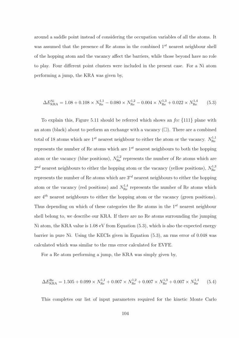
around a saddle point instead of considering the occupation variables of all the atoms. It

was assumed that the presence of Re atoms in the combined 1st nearest neighbour shell

of the hopping atom and the vacancy affect the barriers, while those beyond have no role

to play. Four different point clusters were included in the present case. For a Ni atom

performing a jump, the KRA was given by,

∆ENiKRA = 1.08 + 0.108×N1,1

Re − 0.080×N1,2Re − 0.004×N1,3

Re + 0.022×N1,4Re (5.3)

To explain this, Figure 5.11 should be referred which shows an fcc {111} plane with

an atom (black) about to perform an exchange with a vacancy (�). There are a combined

total of 18 atoms which are 1st nearest neighbour to either the atom or the vacancy. N1,1Re

represents the number of Re atoms which are 1st nearest neighbours to both the hopping

atom or the vacancy (blue positions), N1,2Re represents the number of Re atoms which are

2nd nearest neighbours to either the hopping atom or the vacancy (yellow positions), N1,3Re

represents the number of Re atoms which are 3rd nearest neighbours to either the hopping

atom or the vacancy (red positions) and N1,4Re represents the number of Re atoms which

are 4th nearest neighbours to either the hopping atom or the vacancy (green positions).

Thus depending on which of these categories the Re atoms in the 1st nearest neighbour

shell belong to, we describe our KRA. If there are no Re atoms surrounding the jumping

Ni atom, the KRA value is 1.08 eV from Equation (5.3), which is also the expected energy

barrier in pure Ni. Using the KECIs given in Equation (5.3), an rms error of 0.048 was

calculated which was similar to the rms error calculated for EVFE.

For a Re atom performing a jump, the KRA was simply given by,

∆EReKRA = 1.505 + 0.099×N1,1

Re + 0.007×N1,2Re + 0.007×N1,3

Re + 0.007×N1,4Re (5.4)

This completes our list of input parameters required for the kinetic Monte Carlo

104

Figure 5.11: The fcc {111} plane showing an atom in black next to a vacancy surroundedby other atoms in the 1st nearest neighbour shell. The colour of these atoms representtheir relationship to the black atom and the vacancy. Atoms out of the plane have beenshown smaller in size.

simulation to study the Ni-Re alloy in the non-dilute regime.

105

CHAPTER 6

DIFFUSION IN NON-DILUTE NICKEL-RHENIUMALLOYS

The vacancy diffusion coefficients in non-dilute Ni-Re alloys based on the input parameters

in Chapter 5 was calculated using the kMC code. The Ni as well as the Re tracer diffusion

coefficients were also calculated. The code is capable of handling an fcc simulation cell of

size ≥ 4× 4× 4 with one vacancy for any desired composition, temperature and duration

of kMC simulation.

On running the code, the required simulation cell is generated and the lattice sites

are randomly populated with Ni and Re atoms and a vacancy according to the given

composition. Occupation variables (σi) +1, -1 and 0 represent a Ni atom, a Re atom and

the vacancy respectively. Periodic boundary condition is applied to the simulation cell

and the nearest neighbour relationships are calculated for each lattice position. The initial

energy of the simulation cell is calculated according to the Cluster Expansion method as

described in section 2.3.1 using the ECIs and the EVFE values in Chapter 5, while for

every subsequent kMC step, the energy of the simulation cell is adjusted according to the

changes in the nearest neighbour environment of the vacancy and the jumping atom.

Given the initial configuration of the system, the activation energy barriers ∆Em

corresponding to the 12 possible 1st nearest neighbour vacancy jumps are obtained using

the KRAs calculated in Chapter 5. One of these 12 possible jumps is carried out (see

section 2.2) according to the magnitude of a generated random number, after which the

106

atomic positions are readjusted and the time is updated. The vacancy diffusion coefficient

is calculated according to Equation (2.33). It is noteworthy that instead of tracking the

atomic coordinates throughout the simulation, only the displacements are calculated for

every individual atom and the vacancy from their initial and final position within a kMC

segment. The mean squared displacements are calculated over all the Ni atoms and Re

atoms to obtain their diffusion coefficients according to Equation (2.34). The actual

vacancy concentration, xv in pure Ni, corresponding to a ∆Ef,Ni value of 1.44 eV (see

Table 4.3) has been used in Equation (2.34) for simplicity.

The results presented in this chapter have been calculated for 15× 15× 15 supercells

for five different temperatures (1173 K - 1573 K).

6.1 Error propagation in the calculated diffusivities

The predicted results for diffusivities in the non-dilute systems include the error in the

energy data that are fed as input to the kMC simulations. An analysis of the error

propagation is therefore necessary to understand the impact of these errors on the final

results. Combining Equation (2.37) and Equation (2.40), the activation energy barrier

∆Ea can be given as,

∆Ea = ∆EKRA +1

2(Ef − Ei)

= ∆EKRA +1

2

[(∆Eeff

f +1

2

[ENif (~σ) + ERe

f (~σ)])−(

∆Eeffi +

1

2

[ENii (~σ) + ERe

i (~σ)])]

(6.1)

where ∆EKRA is the Kinetically Resolved Activation Barrier, while Ef and Ei are the

energy of the final and the initial state of the jump. Also, ∆Eeff is the effective vacancy

formation energy and ENi(~σ) and ERe(~σ) are the energies when the vacancy is replaced by

a Ni atom or a Re atom, and are calculated from the binary Cluster Expansion. Again a

107

careful examination of Equation (6.1) tells us that in case of a Ni jump, ENii (~σ) = ENi

f (~σ)

and in the case of a Re jump, ERei (~σ) = ERe

f (~σ) and hence these terms get cancelled.

Furthermore, the remaining ERef (~σ) - ERe

i (~σ) term (or ENif (~σ) - ENi

i (~σ) term in the case

of a Re jump) signify the change in energy due to a Ni-Re swap, while the position of

every other atom remains unchanged. Root mean square errors of 0.048 eV and 0.083 eV

were calculated for the KRAs and EVFEs respectively, while a value of 0.0057 eV/atom

was calculated for the formation energies in the binary CE. This would mean that for a

15× 15× 15 fcc supercell with 13500 atoms, the uncertainty in the total energy predicted

by the CE can be of the order of 77 eV. However, given the terms in the initial and

final states in Equation (6.1) remains the same except for a Ni-Re swap, the systematic

errors get cancelled and the uncertainty in the predicted energy from the CE should be

negligible, given its small rms error when compared to the rms errors for KRA and EVFE.

Thus, to a first approximation, the uncertainty in ∆Ea can be given as [119],

σ(∆Ea) =√

(σ(∆EKRA))2 + 2× 0.52 × (σ(∆Eeff ))2 = ±0.076eV (6.2)

According to Equation (2.11), this should translate to a relative uncertainty in jump

frequency Γ of [119]

σ(Γ)

Γ=

{σ(∆Ea)

kBT

}(6.3)

Thus, the relative uncertainty in jump frequency is a function of temperature alone.

This relative uncertainty in jump frequency is mostly random in nature and one would

expect its effect on the calculated diffusivities to become smaller if the kMC simulations

are run for a long time, as is the case in the propagation of random errors under any

experimental setup. However, analysis of error propagation in the present case is not

straightforward. In addition, one should point out that there might be a component of

systematic error in the evaluation of the barriers, which might have a considerable effect

on the results as resulting inaccuracies would not reduce with longer simulation times.

Looking at Equation (2.33), error propagation in the calculated diffusion coefficients

108

is a combination of the error propagation in t (time elapsed) and the error propagation

in 〈R2(t)〉 (squared displacement). The cumulative jump frequency for the 12 possible

vacancy jumps enter as the reciprocal term in the time step ∆t of the kinetic Monte Carlo

simulation. The relative uncertainty in the time step can be given as [119],

σ(∆t)

∆t=√

12σ(Γ)

Γ(6.4)

The kMC simulations in the present work for the case of non-dilute alloys have been

run for 15 million steps and if one were to look at the relative uncertainty in the diffusivity

coming from the error in time elapsed alone, these are expected to get smaller with the

duration of the kMC simulation.

However, the errors in jump frequency would also mean that there is a degree of un-

certainty in the selection of the vacancy pathway in each kMC step. This implies that the

calculated trajectories of the atoms and vacancies and also their calculated displacements

have a degree of uncertainty. It is difficult to determine if this error is random in nature

and is expected to fade out over the course of a kMC simulation or if the error is expected

to accumulate. To the best knowledge of the author, there were no previous works in

the literature calculating the error propagation in kMC simulations. This is a problem in

vector mathematics and is beyond the scope of this work.

6.2 Results in pure Ni

The pure Ni energy was calculated as -5.4778 eV per atom (pure Re energy was calculated

as -13.39795 eV per atom) from the implementation of the cluster expansion in the kMC

code. This value was constant and did not vary with the simulation cell size. However,

this is 0.0305 eV lower than that calculated by the CASM code (see Table 5.2). We

believe that this difference was due to the difference in the levels of accuracy used in

the two calculations. We used double precision numbers in our kMC code and used the

ECIs (see Table 5.1) without rounding off any digits. The effective vacancy formation

109

Table 6.1: The calculated total energies and vacancy formation energies in pure Ni, ∆Ef,Ni

for different simulation cell sizes (see Equation (2.9))

Simulation Energy (eV) Energy/ Energy (eV) ∆Ef,Ni

cell size (w/o vacancy) atom (eV) (with vacancy) (eV)

4× 4× 4 -1402.3140 -5.4778 -1395.5598 1.27610× 10× 10 -21911.1565 -5.4778 -21904.4023 1.27615× 15× 15 -73950.1547 -5.4778 -73943.4044 1.27220× 20× 20 -175289.2521 -5.4778 -175282.4940 1.280

energy was 10.2413 eV. A vacancy formation energy of 1.28 eV was predicted from a

combination of the binary Ni-Re cluster expansion and EVFE. This is not very different

from the ∆Ef,Ni value of 1.44 eV (see Table 4.3). These numbers have been tabulated for

4 different simulation cell sizes (see Table 6.1). Also ∆Em,i value for Ni was 1.08 eV from

Equation (5.3) on KRAs, same as the results from the first principles calculations.

Given that all these numbers were fairly accurate, we calculated Dv in pure Ni by

running kMC simulations for a total of 109 (1 billion) vacancy jumps. To obtain better

statistics, the kMC trajectory should be divided over a number of segments and Dv

calculated from the time-weighted average of the diffusion coefficients calculated from the

various segments. In order to optimise the kMC segment length, we calculated the Dv in

pure Ni by considering segment lengths of 10, 100, 1000 . . . , 108 and 109 jumps . This

corresponds to a total number of 108, 107, 106,. . . , 10 and 1 segments respectively. The

results are presented in Table 6.2 for the temperature range (1173 K - 1573 K). Also

presented in the table are the results for Dv in pure Ni from analytical formulations using

∆Em,Ni of 1.08 eV. We observe that the results from using a segment length of 10000

jumps matched best with the results of the analytical formulations. Hence, we used a

segment length of 10000 in all the following calculations. It was concluded that the kMC

code works correctly as it was successful in replicating a vacancy correlation factor ≈ 1

in the case of pure Ni. It means the vacancy did indeed undergo a ‘random walk’ in our

kMC simulation.

The self diffusion coefficient in Ni was also calculated and this has been plotted in

110

Figure 6.1 as a function of temperature. The results completely overlap with the previous

results in this work from analytical formulations as well as the kMC code for dilute alloys.

Also, a correlation factor of 0.781 was reproduced in pure Ni reaffirming the validity of

the code. Similarly, the solute diffusion coefficient of Re in Ni was also calculated for

the dilute case using a single Re atom in a 15 × 15 × 15 supercell or an equivalent Re

concentration of 0.0074 at.%. This has been shown as open circles in Figure 6.1. The

results match very well with the results from analytical formulations as well as the kMC

code for dilute alloys.

111

Table 6.2: The calculated Dv in pure Ni for various kMC segment lengths (total number of jumps is 1 billion in each case) comparedto the Dv calculated from analytical formulation with ∆Em,i of 1.08 eV (see Equation (2.6))

Temperature (K) 1173 1273 1373 1473 1573

Dv (m2/s)

Analytical formulation 7.288E-12 1.687E-11 3.456E-11 6.423E-11 1.103E-10

108.097E-12 1.875E-11 3.840E-11 7.136E-11 1.226E-10± 6.781E-17 ± 1.527E-15 ± 6.619E-16 ± 2.237E-15 ± 1.957E-15

1007.361E-12 1.705E-11 3.491E-11 6.485E-11 1.114E-10± 4.801E-16 ± 7.934E-15 ± 1.021E-14 ± 4.397E-14 ± 3.573E-14

10007.298E-12 1.689E-11 3.461E-11 6.423E-11 1.103E-10± 1.925E-15 ± 1.734E-14 ± 2.035E-14 ± 1.069E-13 ± 2.839E-13

kMC10000

7.295E-12 1.690E-11 3.457E-11 6.428E-11 1.103E-10± 7.317E-15 ± 5.663E-14 ± 3.314E-14 ± 8.393E-14 ± 2.733E-14

segment100000

7.233E-12 1.692E-11 3.466E-11 6.413E-11 1.114E-10± 3.076E-14 ± 1.636E-13 ± 6.367E-13 ± 1.556E-13 ± 1.232E-12

length1000000

7.395E-12 1.717E-11 3.543E-11 6.580E-11 1.115E-10± 1.457E-13 ± 6.389E-13 ± 9.790E-13 ± 3.224E-12 ± 2.847E-12

100000007.645E-12 1.735E-11 3.549E-11 6.459E-11 1.130E-10± 1.531E-13 ± 4.009E-13 ± 2.151E-12 ± 3.081E-12 ± 5.014E-12

1000000001.040E-11 2.281E-11 2.338E-11 5.393E-11 1.344E-10± 1.401E-12 ± 3.741E-12 ± 6.459E-12 ± 6.090E-12 ± 1.667E-11

10000000001.219E-11 2.184E-11 6.332E-12 7.792E-11 1.519E-10± 2.907E-12 ± 1.277E-11 ± 7.885E-12 ± 1.416E-11 ± 1.813E-11

112

Figure 6.1: The self-diffusion coefficient in Ni and Re diffusion coefficient in Ni as a func-tion of temperature. The open symbols represent the results from the kMC simulationsusing our code for non-dilute alloys, the filled symbols represent the results from the kMCsimulations using the code provided by Dr. Sergej Schuwalow for dilute alloys and thelines represent the results calculated from Lidiard’s model

6.3 Results in non-dilute Ni-Re alloys

It must be pointed out that the kMC simulations performed in pure Ni only took a

few minutes to complete 1 billion vacancy jumps. This was because the energy of the

simulation cell and the ∆Em,Ni both remain fixed. However in the case of non-dilute

alloys of Ni-Re, the energy and the ∆Em,i have to be calculated at each step.

kMC simulations were run for the non-dilute Ni-Re alloys for 15 million vacancy jumps.

These simulations running on single processors took 36 hours on an average to complete.

The compositions probed were 1 at.%, 2 at.%, 3 at.%, 4 at.%, 5 at.%, 6.25 at. %, 7.5 at.%,

8.75 at. % and 10 at.% Re in binary alloys with Ni. This was because the concentration

113

of Re in the γ phase even in the third generation of most Ni-based superalloys does not

exceed 10 at.% [115]. Multiple trials were run for each of these compositions for better

statistics. The segment length chosen was 10000 vacancy jumps as deduced from the

results on pure Ni.

6.3.1 Monte Carlo simulations

In order to arrive at the thermodynamically most stable configurations for the non-dilute

Ni-Re systems, Monte Carlo simulations using the Metropolis algorithm [68] were run. An

initial random configuration was chosen for the system and its energy calculated. At each

step of the Monte Carlo simulation, an atom was swapped with another dissimilar atom

in the system chosen at random and the energy of the system was recalculated. If the

swap led to a decrease in the energy of the system, the new configuration was accepted.

If the swap led to an increase in the energy of the system, a random number R, where

0<R<1 was generated and the new configuration was accepted if

R < exp

(−∆U

kBT

)(6.5)

where ∆U is the difference in energy of the system due to the swap, kB is the Boltzmann

constant and T is the absolute temperature of the system. If this was not the case, the old

configuration was kept. In one Monte Carlo cycle, the simulation run through each atom

in the system, and several such cycles were run until the energy of the system converged.

Figure 6.2 shows the results obtained for a Ni alloy containing 5 at.% Re at 1373

K. Figure 6.2a shows the initial random distribution of Re atoms in the 15× 15× 15 fcc

supercell of Ni, while Figure 6.2b represents the configuration after 100 Monte Carlo cycles

showing that almost all of the Re atoms have clustered together. The cluster of Re atoms

appears as fragments, but they can be visualized together as a single cluster considering

images of the supercell across periodic boundaries. The results from Figure 6.3 show that

the energy of the system has converged in less than 100 Monte Carlo cycles. Similar

114

results were obtained for Monte Carlo simulations performed at different temperatures as

well as for different compositions. In all the cases, the Re atoms clustered together at the

end of the Monte Carlo simulations, suggesting that Re would completely phase separate

in an alloy with Ni.

The magnitudes of the ECIs obtained in the present work did in fact indicate the

formation of Re clusters, and it was also seen that the binding energies increased from Re

pairs to triplets to quadruplets. From the available Ni-Re phase diagrams [25], clustering

can be expected at lower temperatures as the solubility of Re in Ni significantly falls

down, however at higher temperatures Re is expected to be present in the solution with

Ni. Results from previous Monte Carlo works [32] have however indicated the presence

of short range ordering at lower temperatures, but the ordering again vanishes at higher

temperatures. Results from 3D atom probe analysis [26, 27] have also shown that Re

atoms are randomly distributed in Ni and neither clustering or ordering is present at

high temperatures. Similarly, results from EXAFS experiments [28] show that Re is

coordinated by 12 Ni atoms. All this is in contrast to the findings of the present work

where Re is not randomly distributed in Ni even at high temperatures. The cluster

expansion in the present work found D1a-Ni4Re to be the most stable phase amongst the

configurations considered in the first principles dataset. However, unlike the results of

Maisel et al [32], the Monte Carlo simulations failed to predict the formation of this phase.

This brings out the limitations of the calculated ECIs in the present work. However, it

must be noted that the first principles dataset used in the work of Maisel et al [32] was

larger than used in the present work. Also, they performed high-throughput calculations

on supercells of up to 20 atoms to fit their ECIs. In comparison, supercells of only up to 10

atoms were used in the present work due to the limitations of the available computational

resources.

However, while Re clustering was observed in the case of MC simulations, this is

highly unlikely to occur over the course of a typical kMC simulation of 15 million jumps

as used in the present work and it is expected that the Re distribution would not change

115

(a) Random distribution of Re atoms at the beginning of the Monte Carlo simulation

(b) Clustered Re atoms at the end of the Monte Carlo simulation

Figure 6.2: Changes in the configuration of Re atoms for a binary Ni alloy containing 5at.% Re during the course of the Monte Carlo simulation at 1373 K. The size of the fccsimulation cell is 15× 15× 15 and the Ni atoms have been deleted for clarity. a, b and crepresent the three orthogonal directions.

116

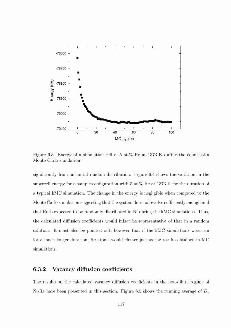
Figure 6.3: Energy of a simulation cell of 5 at.% Re at 1373 K during the course of aMonte Carlo simulation

significantly from an initial random distribution. Figure 6.4 shows the variation in the

supercell energy for a sample configuration with 5 at.% Re at 1373 K for the duration of

a typical kMC simulation. The change in the energy is negligible when compared to the

Monte Carlo simulation suggesting that the system does not evolve sufficiently enough and

that Re is expected to be randomly distributed in Ni during the kMC simulations. Thus,

the calculated diffusion coefficients would infact be representative of that in a random

solution. It must also be pointed out, however that if the kMC simulations were run

for a much longer duration, Re atoms would cluster just as the results obtained in MC

simulations.

6.3.2 Vacancy diffusion coefficients

The results on the calculated vacancy diffusion coefficients in the non-dilute regime of

Ni-Re have been presented in this section. Figure 6.5 shows the running average of Dv

117

Figure 6.4: Energy of a simulation cell of 5 at.% Re at 1373 K as a function of kMCsimulation time (the energy scale has been kept the same as in Figure 6.3 for comparison)

for an alloy with 5 at.% Re at 1373 K over the course of a typical kMC simulation of 15

million vacancy jumps. The Dv value has converged confirming that the duration of the

kMC simulations performed in the present work was sufficient.

Figure 6.6 shows the calculated vacancy diffusion coefficients in the non-dilute regime

at 1373 K. Several kMC simulations were run for each composition and the mean Dv

was calculated. The variation in the results was small, as can be seen from the error

bars in Figure 6.6, where the error bars represent the standard deviation from the mean

Dv. A linear trend was observed for the entire composition range. This is surprising

as it suggests that interactions between Re atoms have no additional effects on vacancy

diffusivity. An addition of 10 at.% Re is expected to reduce the Dv in Ni by 36 %.

118

Figure 6.5: The running average of the vacancy diffusion coefficient for an alloy with 5at.% Re at 1373 K as a function of simulation time

Figure 6.6: Calculated Dv in the non-dilute regime in Ni-Re at 1373 K

119

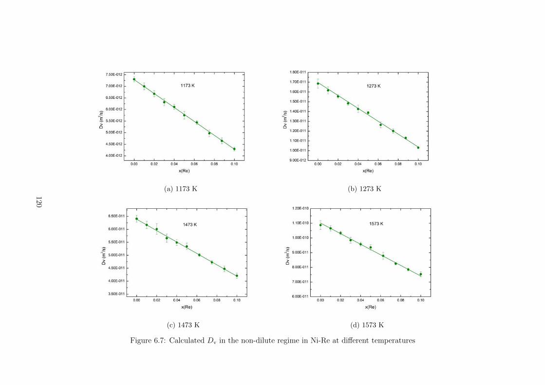
(a) 1173 K (b) 1273 K

(c) 1473 K (d) 1573 K

Figure 6.7: Calculated Dv in the non-dilute regime in Ni-Re at different temperatures

120

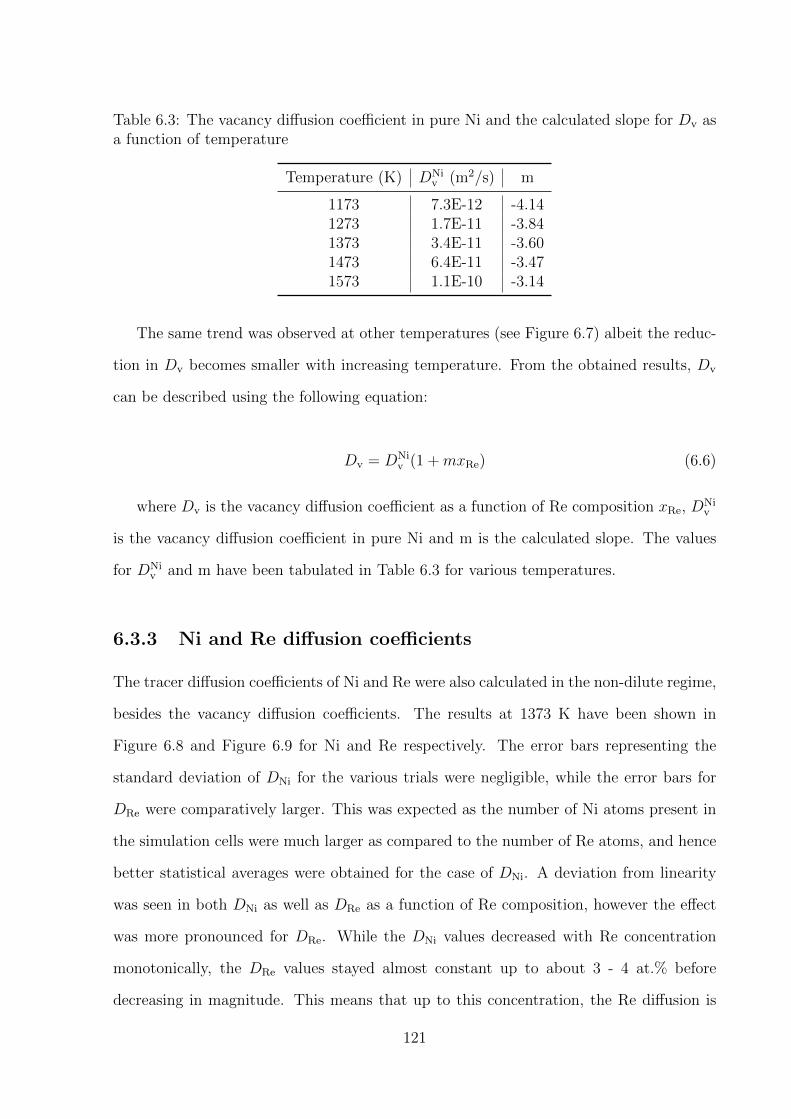
Table 6.3: The vacancy diffusion coefficient in pure Ni and the calculated slope for Dv asa function of temperature

Temperature (K) DNiv (m2/s) m

1173 7.3E-12 -4.141273 1.7E-11 -3.841373 3.4E-11 -3.601473 6.4E-11 -3.471573 1.1E-10 -3.14

The same trend was observed at other temperatures (see Figure 6.7) albeit the reduc-

tion in Dv becomes smaller with increasing temperature. From the obtained results, Dv

can be described using the following equation:

Dv = DNiv (1 +mxRe) (6.6)

where Dv is the vacancy diffusion coefficient as a function of Re composition xRe, DNiv

is the vacancy diffusion coefficient in pure Ni and m is the calculated slope. The values

for DNiv and m have been tabulated in Table 6.3 for various temperatures.

6.3.3 Ni and Re diffusion coefficients

The tracer diffusion coefficients of Ni and Re were also calculated in the non-dilute regime,

besides the vacancy diffusion coefficients. The results at 1373 K have been shown in

Figure 6.8 and Figure 6.9 for Ni and Re respectively. The error bars representing the

standard deviation of DNi for the various trials were negligible, while the error bars for

DRe were comparatively larger. This was expected as the number of Ni atoms present in

the simulation cells were much larger as compared to the number of Re atoms, and hence

better statistical averages were obtained for the case of DNi. A deviation from linearity

was seen in both DNi as well as DRe as a function of Re composition, however the effect

was more pronounced for DRe. While the DNi values decreased with Re concentration

monotonically, the DRe values stayed almost constant up to about 3 - 4 at.% before

decreasing in magnitude. This means that up to this concentration, the Re diffusion is

121

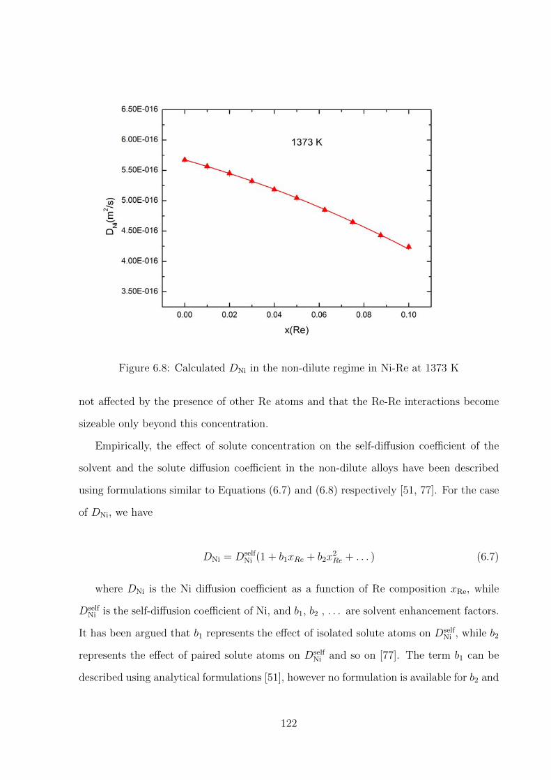
Figure 6.8: Calculated DNi in the non-dilute regime in Ni-Re at 1373 K

not affected by the presence of other Re atoms and that the Re-Re interactions become

sizeable only beyond this concentration.

Empirically, the effect of solute concentration on the self-diffusion coefficient of the

solvent and the solute diffusion coefficient in the non-dilute alloys have been described

using formulations similar to Equations (6.7) and (6.8) respectively [51, 77]. For the case

of DNi, we have

DNi = DselfNi (1 + b1xRe + b2x

2Re + . . . ) (6.7)

where DNi is the Ni diffusion coefficient as a function of Re composition xRe, while

DselfNi is the self-diffusion coefficient of Ni, and b1, b2 , . . . are solvent enhancement factors.

It has been argued that b1 represents the effect of isolated solute atoms on DselfNi , while b2

represents the effect of paired solute atoms on DselfNi and so on [77]. The term b1 can be

described using analytical formulations [51], however no formulation is available for b2 and

122

Figure 6.9: Calculated DRe in the non-dilute regime in Ni-Re at 1373 K

higher order terms. Given a deviation from linearity was clearly observed, we have done

a parabolic fit of the DNi data and considered two terms in the Equation (6.7). These

fitting parameters have been tabulated in Table 6.4.

Similarly for the case of DRe, we have

DRe = DdiluteRe (1 +B1xRe +B2x

2Re + . . . ) (6.8)

where DRe is the Re diffusion coefficient as a function of Re composition xRe, while

Table 6.4: The self-diffusion coefficient in pure Ni and the calculated solvent enhancementfactors for DNi as a function of temperature

Temperature (K) DselfNi m2/s b1 b2

1173 1.50E-17 -2.22 -9.811273 1.06E-16 -2.02 -8.061373 5.67E-16 -1.82 -7.671473 2.41E-15 -1.68 -6.341573 8.51E-15 -1.53 -6.38

123

Table 6.5: The Re diffusion coefficient in the dilute case and the calculated solute en-hancement factors for DRe as a function of temperature

Temperature (K) DdiluteRe m2/s B1 B2

1173 1.03E-19 0.44 -20.871273 1.07E-18 0.73 -23.991373 7.82E-18 1.28 -28.951473 4.29E-17 1.39 -27.921573 1.95E-16 1.40 -27.23

DdiluteRe represents the Re diffusion coefficient in Ni for the dilute case, and B1, B2, . . . are

solute enhancement factors. The DRe data was also fit to a parabola and these values

have been tabulated in Table 6.5. The values for DRe at the Re concentration of 1 at.%

were taken as DdiluteRe in the present case.

The calculated DNi and DRe values from the kMC simulations at other temperatures

have also been shown in Figure 6.10 and Figure 6.11 respectively.

124

(a) 1173 K (b) 1273 K

(c) 1473 K (d) 1573 K

Figure 6.10: Calculated DNi in the non-dilute regime in Ni-Re at different temperatures

125

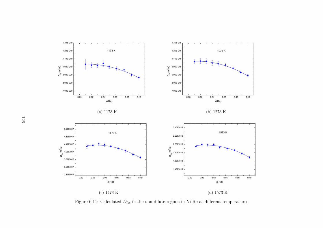
(a) 1173 K (b) 1273 K

(c) 1473 K (d) 1573 K

Figure 6.11: Calculated DRe in the non-dilute regime in Ni-Re at different temperatures

126

6.3.4 Correlation factors

The correlation factors were also calculated from the kMC simulations for the vacancy,

the Ni as well as the Re atoms. In the case where an atom or a vacancy does not perform

a true random jump, its jump is said to be correlated and its mean square displacement

is given as,

< |R|2 >= fnλ2 (6.9)

Here, λ is the jump distance, given as a/√

2 , where a is the Ni lattice parameter and n

is the number of jumps. Rearranging the Equation (6.9) gives f as,

f =2

n

< |R|2 >a2

(6.10)

The kMC simulation was divided over a number of segments and the calculated f values

were averaged over these segments. Calculated fv, fNi and fRe values for various Ni-Re

compositions at 1373 K have been plotted in Figure 6.12. The trend in fv looks similar to

that of Dv at 1373 K (see Figure 6.6). This is expected as Dv is directly proportional to fv

(see Equation (2.18)). fv is close to unity for pure Ni, and the value gradually drops with

increasing Re concentration. However, the decrease in fv is more pronounced than that

predicted by the Manning’s model (see Figure 4.7) which predicted a negligible effect of

Re concentration on fv. An addition of 10 at.% Re brings down the fv to approximately

0.75, implying moderate correlation effects.

An fNi value of 0.78 was calculated for pure Ni, which matches the value in the

literature accurately [58]. The fNi value decreased linearly with the Re concentration to

about 0.62 for 10 at.% Re. This is expected as a reverse jump after a Ni-� exchange

becomes more likely if the Ni atom is surrounded by more Re atoms, given the low value

for the Re-� exchange frequency. As a result, the efficiency of the Ni diffusion is reduced.

In the case of Re, the fRe values could not be calculated up to 5 at.% Re. This is

because given the low frequency for a Re-� exchange, if the Re atoms do not perform a

127

single jump in an entire kMC segment, the fRe value for that segment becomes undefined,

thus giving an error in the overall fRe value. This becomes less likely with increasing Re

concentration, as is seen to be the case beyond 5 at.% Re. This is in contrast to the

calculation of DRe, where the mean of the squared displacement is taken over all the Re

atoms in the system, thus giving a well-defined value even for the case of dilute alloys.

The calculated fRe value was 0.995 for 6.25 at.% Re and dropped only to 0.991 for

10 at.% Re. Thus, effectively the Re diffusive jumps were uncorrelated throughout the

investigated composition range, which matches the results from the Lidiard’s model (see

Figure 4.4).

Figure 6.12: Calculated correlation factors in the non-dilute regime in Ni-Re at 1373 K

6.3.5 Variation of D0 and Q as a function of composition

For pure Ni, the D0 and Q values can be described using analytical formulations. However,

for alloys of Re in Ni, it is difficult to predict these values from analytical formulations,

given their complex dependence on temperature. These values were extracted from the

128

intercepts and the slopes respectively of the lnD versus 1/T curves for the different com-

positions and have been plotted in Figure 6.13 and 6.14 as a function of composition.

In pure Ni, the calculated Dv0 value was 3.03 × 10−7 m2/s and Qv value was 1.075 eV,

compared to the expected Dv0 value of 2.81 × 10−7 m2/s (a2 × ν∗Ni) and Qv value of 1.08

eV. DNi0 and QNi values were 10.1 × 10−7 m2/s and 2.52 eV respectively and matched

the expected values from analytical formulations exactly (see Table 4.3). A DRe0 value of

7.7 × 10−7 m2/s and QRe value of 2.99 eV was calculated for 1 at.% Re in Ni and these

values also matched the expected values for dilute alloys of Re in Ni(see Table 4.3).

While the Dv0 curve showed no trend with increasing Re concentration, the Qv values

increased almost linearly with the Re concentration. Re, having a ∆Em value of 1.51 eV

compared to a value of 1.08 eV for pure Ni, is expected to increase the overall Qv value in

alloys with Ni. A Qv value of 1.14 eV was calculated for 10 at.% Re clearly demonstrating

that the vacancy diffusion becomes slower with increasing amount of Re.

Both the DNi0 and QNi values increased with the Re concentration. While the DNi

0

value at 10 at.% Re was about 1.2 times the value in pure Ni, the QNi value increased

from 2.52 eV to about 2.57 eV, which is equivalent to a decrease in the diffusivity by a

factor of approximately 0.65 at a temperature of 1373 K.

However, no trend was observed for the case of DRe0 and QRe. This can be attributed

to the large standard deviations in the calculated DRe data. A smaller value for Re-�

exchange frequency complemented with the smaller number of Re atoms in the simulation

cells result in fewer Re jumps over the course of a kMC simulation. This leads to relatively

inferior statistics when compared to the case of Ni. It must be noted that D0 and Q values

are highly sensitive to the calculated diffusion coefficients, and hence more precision is

required in the diffusion coefficients data when deducing the D0 and Q values accurately

is the main objective. This would require running the kMC simulations for many more

times or for longer durations.

129

(a) Calculated DNi0 as a function of Re composition

(b) Calculated DRe0 as a function of Re composition

(c) Calculated Dv0 as a function of Re composition

Figure 6.13: Calculated diffusion pre-factors as a function of Re composition in Ni

130

(a) Calculated QNi as a function of Re composition

(b) Calculated QRe as a function of Re composition

(c) Calculated Qv as a function of Re composition

Figure 6.14: Calculated activation energies as a function of Re composition in Ni

131

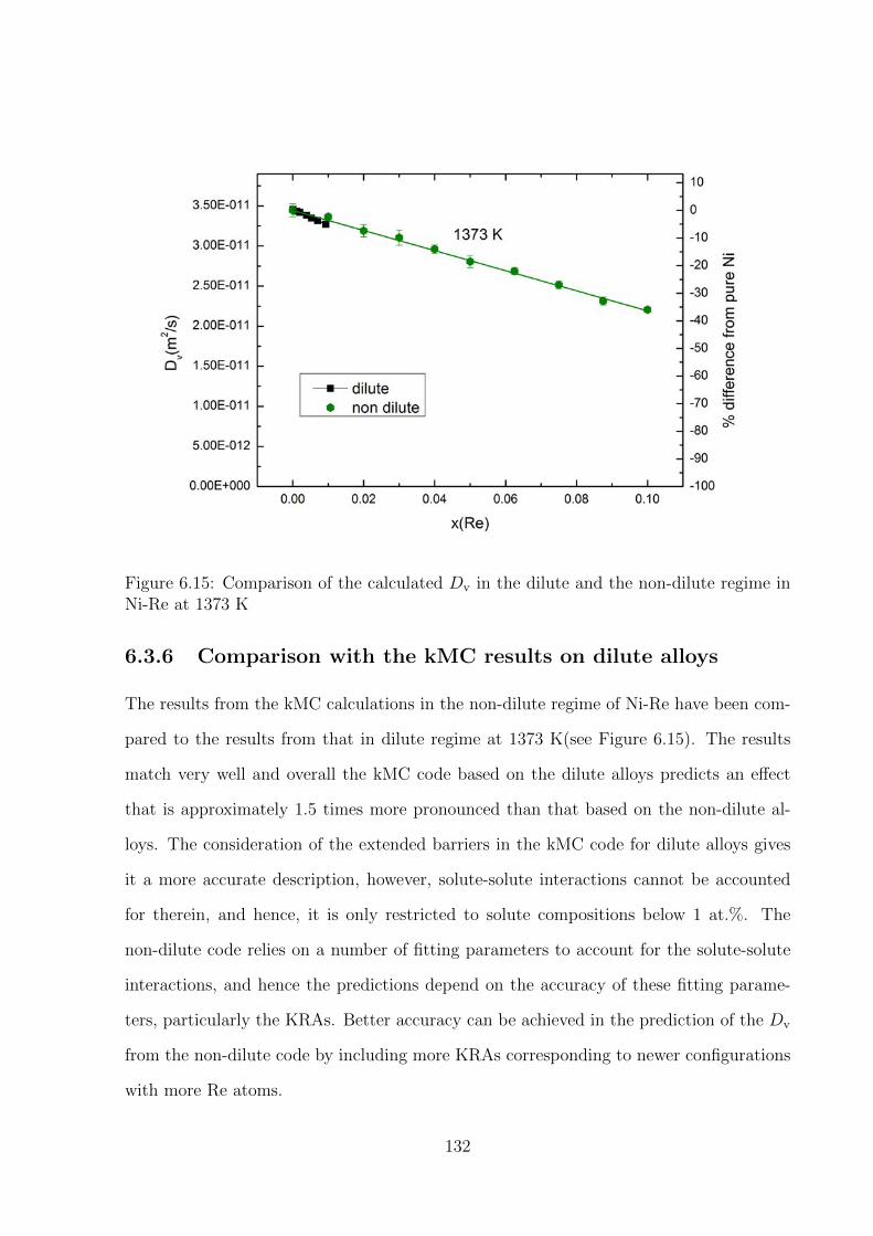
Figure 6.15: Comparison of the calculated Dv in the dilute and the non-dilute regime inNi-Re at 1373 K

6.3.6 Comparison with the kMC results on dilute alloys

The results from the kMC calculations in the non-dilute regime of Ni-Re have been com-

pared to the results from that in dilute regime at 1373 K(see Figure 6.15). The results

match very well and overall the kMC code based on the dilute alloys predicts an effect

that is approximately 1.5 times more pronounced than that based on the non-dilute al-

loys. The consideration of the extended barriers in the kMC code for dilute alloys gives

it a more accurate description, however, solute-solute interactions cannot be accounted

for therein, and hence, it is only restricted to solute compositions below 1 at.%. The

non-dilute code relies on a number of fitting parameters to account for the solute-solute

interactions, and hence the predictions depend on the accuracy of these fitting parame-

ters, particularly the KRAs. Better accuracy can be achieved in the prediction of the Dv

from the non-dilute code by including more KRAs corresponding to newer configurations

with more Re atoms.

132

6.3.7 Discussion

Having calculated the vacancy diffusion coefficients in the dilute as well as non-dilute

regime for Ni-Re alloys, its application to a creep model needs to be verified. It must

be reiterated that Ni-based superalloys are used in high temperature applications where

creep is the main deformation mechanism. One commonly used creep model is shown in

Equation (6.11) [51],

ε = A2Deff

[γSFEGb

]n [ σE

]m(6.11)

where A2, n and m are structure dependent fitting parameters, Deff is the effective

diffusion coefficient, γSFE is the stacking fault energy, σ is the applied stress, b is the

Burgers vector, G is the shear modulus and E is the Young’s modulus. Other models

such as the one used by Zhu et al [38] also include superalloy microstructural factors like

γ′ size and volume fraction. Most of these factors are composition dependent and also

vary with temperature. Thus, in order to study the effect of one of these factors on the

creep rate, all the other factors, in principle have to be constant.

In the present work, we were interested in studying the effect of composition on Deff,

which determines the rate of mass transport in the alloy. However, there is no unique

formulation for calculating Deff [120, 121, 122, 123] and in the present work, we have

argued that Dv is an equivalent measure of Deff. Indeed, the atomic mass transport is

counter-balanced by the diffusion of vacancies and the net flux of vacancies is equal and

opposite to the net flux of atoms in the alloy. Vacancies have to diffuse from emitting

dislocation cores to absorbing dislocation cores through the γ matrix for climb to continue

at the γ/γ′ interface during creep.

For the case of pure Ni, Deff would be the same as DNi. Comparing Equations (2.6)

and (2.18) in pure Ni, we have,

Dv =DNi

xv,Ni

fv

fNi

(6.12)

133

From Figure 6.12, the ratio of fv to fNi is approximately constant at about 1.25

throughout the probed composition range. If the concentration of vacancies, xv,i in the

alloy is also assumed to be constant, then extending Equation (6.12) to an alloy of Ni, we

have

Dv ∝ Deff (6.13)

It means that the relative effect of the alloy composition on Dv should be the same

as Deff. However, it must be kept in mind that since xv,Ni is very small in magnitude (≈

10−5) even at high temperatures, Deff and Dv would differ by orders of magnitude. Indeed,

vacancies have to diffuse for much longer distances through the lattice compared to the

individual atoms. Nevertheless, having established that the effective diffusion coefficient

is proportional to the vacancy diffusion coefficient to a first approximation, we calculated

vacancy diffusion coefficients in the present work. Also, in Chapter 1, the role of vacancies

in determining the rate of dislocation climb was discussed and the beneficial role of Re

additions was attributed to its possible slowing down of the rate of vacancy diffusion,

while its effect on other factors was found to be minimal.

Again, it has been found that the creep strain rate ε is inversely proportional to the

time to rupture tr of the superalloy component. Thus, we have

ε× tr = B (6.14)

where B is a constant. This is called the Monkman-Grant relationship [1]. Comparing

Equations (6.11),(6.13) and (6.14), we have

Dv ∝1

tr(6.15)

We use this relationship to validate the creep results of Blavette et al [12] conducted

on two different Ni-based superalloys, CMSX-2 and PWA 1480 at a temperature of 1123

K and an applied stress of 500 MPa. Re additions were made to these first generation

134

superalloys at the expense of W partially or completely. The corresponding Re composi-

tion in the γ phase, xRe and time to rupture, tr for these superalloys before and after Re

addition have been tabulated in Table 6.6. The superalloy samples were heat treated at

the same temperature as the creep tests, and hence the xRe values represent the actual

Re composition of the alloy at the creep temperature. Given that all other factors remain

unchanged, the increase in creep lives should be attributed to the change in Dv by the Re

addition. Table 6.7 shows the Dv values calculated in the binary Ni-Re alloys for pure Ni,

3 at.% Re and 4 at.% Re at 1173 K, which closely resemble the investigated superalloys.

The calculated decrease in Dv accounts for about three-fifth of the decrease in tr−1 in

both the cases. This largely explains the origin of the Re-effect in these alloys.

Again, from the calculation of Dv using the code for dilute alloys (see Figure 4.11),

it was found that W has the same potency as Re as far as reduction in Dv is concerned.

Thus, given that Re additions were made to these alloys at the expense of W, one can

justify the improvement in creep lives to the fact that Re partitioning to the γ phase is

stronger than W. Indeed, while the W concentration in the γ phase of PWA 1480 alloy

was 2.15 at.%, on being replaced by Re completely in the PWA 1480+Re alloy, the Re

concentration in the γ phase was 3.71 at.%. Thus, the Re-effect should be explained in

totality by its slowing down of the vacancy diffusion together with strong partitioning to

the γ phase.

It must be pointed out that validation of our results would require agreement with

more creep data on superalloys from a number of sources. However, it is important to

understand that the number of variables in superalloys metallurgy is very large, and

hence availability of creep data where most variables have been kept fixed is difficult.

For example, adding or removing one element at the expense of other does change the

partitioning of all the elements, the volume fraction of γ′ as well as the elastic properties.

Furthermore, the phase composition data is not available for the majority of the creep

experiments and the authors tend to fit their creep models to the overall composition

instead of the γ composition.

135

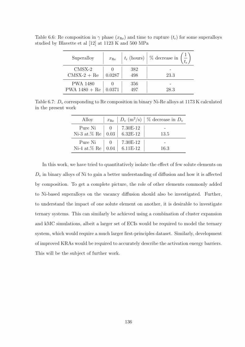
Table 6.6: Re composition in γ phase (xRe) and time to rupture (tr) for some superalloysstudied by Blavette et al [12] at 1123 K and 500 MPa

Superalloy xRe tr (hours) % decrease in

(1

tr

)CMSX-2 0 382 -

CMSX-2 + Re 0.0287 498 23.3

PWA 1480 0 356 -PWA 1480 + Re 0.0371 497 28.3

Table 6.7: Dv corresponding to Re composition in binary Ni-Re alloys at 1173 K calculatedin the present work

Alloy xRe Dv (m2/s) % decrease in Dv

Pure Ni 0 7.30E-12 -Ni-3 at.% Re 0.03 6.32E-12 13.5

Pure Ni 0 7.30E-12 -Ni-4 at.% Re 0.04 6.11E-12 16.3

In this work, we have tried to quantitatively isolate the effect of few solute elements on

Dv in binary alloys of Ni to gain a better understanding of diffusion and how it is affected

by composition. To get a complete picture, the role of other elements commonly added

to Ni-based superalloys on the vacancy diffusion should also be investigated. Further,

to understand the impact of one solute element on another, it is desirable to investigate

ternary systems. This can similarly be achieved using a combination of cluster expansion

and kMC simulations, albeit a larger set of ECIs would be required to model the ternary

system, which would require a much larger first-principles dataset. Similarly, development

of improved KRAs would be required to accurately describe the activation energy barriers.

This will be the subject of further work.

136

CHAPTER 7

CONCLUSIONS AND SCOPE FOR FUTUREWORK

In this thesis, the effect of solute atoms on diffusional processes was investigated using

a variety of computational methods. Analytical approximations were used to study the

effect of dilute levels of Re, W and Ta on the diffusivities of vacancies in fcc Ni. Results

from analytical formulations were compared to kinetic Monte Carlo simulations performed

based on data obtained from density functional theory. This was done to attempt to

explain how composition may affect the climb of dislocations at the γ/γ′ interfaces, with

ramifications on creep properties.

Results for diffusivity in the dilute regime suggest the relationship between vacancy

diffusivity and solute content for all elements considered is linear in nature. It is apparant

from the dilute results that there is a discrepancy between the analytical model and

the kinetic Monte Carlo simulations. This is due to several simplifying assumptions

in the analytical model, while the kinetic Monte Carlo simulations explicitly included

the diffusion processes to accurately describe the systems. The magnitude of the effect

predicted by the kinetic Monte Carlo simulations is appreciable in size, however, the

concentration of solute elements in the γ phase of Ni-based superalloys is such that solute-

solute interactions must be considered to account for the non-dilute concentrations in the

relevant phase.

To that effect, this work was extended to consider diffusivity in non-dilute systems

137

using kinetic Monte Carlo simulations. In order to consider the energetics of a complex

binary system, the cluster expansion was employed to efficiently calculate the total energy

of a configuration of atoms on the fcc lattice while the values of migration energy barriers

were also cluster expanded considering first neighbours only. Non-dilute results suggest

that solute-solute interactions have minimal effects on vacancy diffusivity. It should be

pointed out, however that the reliance of these results on accurate effective cluster inter-

actions and cluster expanded migration barriers means that some inaccuracy should be

expected.

Such a comprehensive study of the effect of solute content on vacancy diffusivity and

solute/solvent diffusivity in the non-dilute regime has not been carried out in superalloys

field and helps to clarify how Re may affect the creep properties in these materials. Indeed,

several authors have suggested that the renowned Re-effect could be attributed to the

fact that Re, the slowest diffusing solute in Ni-based superalloys, slows down diffusional

processes required for dislocation climb. This work indicates that, while Re additions slow

down vacancy diffusivity in these alloys, its effect is similar to W. Hence, a key aspect of

the beneficial impact of Re additions on creep properties is that Re strongly partitions to

the γ phase in superalloys where dislocation climb occurs.

The results of this work were used to rationalise the improvements in creep life of

Re containing alloys using simple well-recognised models for predicting creep strain rate.

These show that the beneficial effects of Re on the creep properties of Ni-based superalloys

can be partially accounted for by the effect of Re on diffusional processes. However, it

should be pointed out that whenever alloy compositions are modified to investigate the role

of solute elements on creep, several variables are modified at once. Indeed, small additions

of Re are known to reduce γ′ phase fraction, increase lattice misfit, retard rafting and

affect dislocation processes in the γ phase. Therefore, careful experimentation to evaluate

each of these effects independently would be desirable.

In terms of future work, there are several areas where the present research can be

improved upon. Re clustering in Ni should be investigated in more detail to resolve the

138

discrepancy between different studies. The calculation of non-dilute diffusivities should

be extended to treat ternary systems, which would require effective cluster interaction

coefficients and kinetically resolved activation barriers fit against a larger dataset. Dif-

fusion calculations, especially in the non-dilute regime must also be performed on other

alloying elements commonly added to Ni-based superalloys. This is desirable in order to

get a complete picture of the effect of chemistry on creep in superalloys.

139

LIST OF REFERENCES

[1] R. C. Reed. The superalloys: fundamentals and applications. Cambridge UniversityPress, 2006.

[2] A. Mottura and R. C. Reed. What is the role of rhenium in single crystal superalloys?MATEC Web of Conferences, 14:01001, 2014.

[3] G. E. Dieter. Mechanical metallurgy. McGraw-Hill series in materials science andengineering. McGraw-Hill, 1986.

[4] V. Paidar, D. P. Pope, and V. Vitek. A theory of the anomalous yield behavior inL12 ordered alloys. Acta Metallurgica, 32(3):435–448, 1984.

[5] C. M. F. Rae and R. C. Reed. The precipitation of topologically close-packed phasesin rhenium-containing superalloys. Acta Materialia, 49(19):4113 – 4125, 2001.

[6] G. A. Whittaker. Precision casting of aero gas turbine components. MaterialsScience and Technology, 2(5):436–441, 1986.

[7] Y. Amouyal, Z. Mao, and D. N. Seidman. Effects of tantalum on the partition-ing of tungsten between the γ and γ′-phases in nickel-based superalloys: linkingexperimental and computational approaches. Acta Materialia, 58(18):5898–5911,2010.

[8] A. F. Giamei. Deformation and fracture of advanced anisotropic superalloys.AFOSR Annual Report FR-11009, 1978.

[9] A. Sato, H. Harada, T. Yokokawa, T. Murakumo, Y. Koizumi, T. Kobayashi, andH. Imai. The effects of ruthenium on the phase stability of fourth generation Ni-basesingle crystal superalloys. Scripta Materialia, 54(9):1679 – 1684, 2006.

[10] N. Matan, D. C. Cox, C. M. F. Rae, and R. C. Reed. On the kinetics of rafting inCMSX-4 superalloy single crystals. Acta Materialia, 47(7):2031–2045, 1999.

140

[11] A. F. Giamei and D. L. Anton. Rhenium additions to a Ni-base superalloy: effectson microstructure. Metallurgical Transactions A, 16(11):1997–2005, 1985.

[12] D. Blavette, P. Caron, and T. Khan. An atom probe investigation of the role ofrhenium additions in improving creep resistance of Ni-base superalloys. ScriptaMetallurgica, 20(10):1395 – 1400, 1986.

[13] D. Blavette, P. Caron, and T. Khan. An atom-probe study of some fine-scalemicrostructural features in Ni-based single crystal superalloys. In S. Reichman,D. N. Duhl, G. Maurer, S. Antolovich, and C. Lund, editors, Superalloys 1988,pages 305–314. The Minerals, Metals and Materials Society, Warrendale, PA, USA,1988.

[14] J. Li, D. Tang, R. Lao, S. Liu, and Z. Wu. Effects of rhenium on creep rupturelife of a single crystal superalloy. Journal of Materials Science and Technology,15(1):53–57, 1999.

[15] S. Wollmer, T. Mack, and U. Glatzel. Influence of tungsten and rhenium concen-tration on creep properties of a second generation superalloy. Materials Science andEngineering: A, 319-321:792–795, 2001.

[16] A. C. Yeh and S. Tin. Effects of Ru and Re additions on the high temperature flowstresses of Ni-base single crystal superalloys. Scripta Materialia, 52(6):519–524,2005.

[17] B. Gan and S. Tin. Assessment of the effectiveness of transition metal so-lutes in hardening of Ni solid solutions. Materials Science and Engineering: A,527(26):6809–6815, 2010.

[18] J. P. Hirth and J. Lothe. Theory of dislocations. Krieger Publishing Company,Malabar, Florida, 1982.

[19] A. Mottura. Analysis of atomic-scale phenomena and the rhenium-effect in nickelbased superalloys. PhD thesis, Imperial College London, 2009.

[20] S. L. Shang, C. L. Zacherl, H. Z. Fang, Y. Wang, Y. Du, and Z. K. Liu. Effects ofalloying element and temperature on the stacking fault energies of dilute Ni-basesuperalloys. Journal of Physics: Condensed Matter, 24(50):505403, 2012.

141

[21] X. X. Yu and C. Y. Wang. The effect of alloying elements on the dislocation climbingvelocity in Ni: a first-principles study. Acta Materialia, 57(19):5914–5920, 2009.

[22] F. Pettinari, J. Douin, G. Saada, P. Caron, A. Coujou, and N. Clement. Stackingfault energy in short-range ordered γ-phases of Ni-based superalloys. MaterialsScience and Engineering: A, 325(1-2):511–519, 2002.

[23] F. Diologent and P. Caron. On the creep behavior at 1033K of new generationsingle-crystal superalloys. Materials Science and Engineering: A, 385(1):245–257,2004.

[24] N. Wanderka and U. Glatzel. Chemical composition measurements of a nickel-basesuperalloy by atom probe field ion microscopy. Materials Science and Engineering:A, 203(1-2):69–74, 1995.

[25] H. Okamoto. Ni-Re (nickel-rhenium). Journal of Phase Equilibria and Diffusion,33(4):346–346, 2012.

[26] A. Mottura, M. K. Miller, and R. C. Reed. Atom probe tomography analysis ofpossible rhenium clustering in nickel-based superalloys. In R. C. Reed, P. Caron,T. Gabb, E. Huron, and S. Woodard, editors, Superalloys 2008, pages 891 – 900.The Minerals, Metals and Materials Society, 2008.

[27] A. Mottura, N. Warnken, M. K. Miller, M. W. Finnis, and R. C. Reed. Atom probetomography analysis of the distribution of rhenium in nickel alloys. Acta Materialia,58(3):931–942, 2010.

[28] A. Mottura, R. T. Wu, M. W. Finnis, and R. C. Reed. A critique of rhenium cluster-ing in Ni-Re alloys using extended X-ray absorption spectroscopy. Acta Materialia,56(11):2669–2675, 2008.

[29] A. Mottura, M. W. Finnis, and R. C. Reed. On the possibility of rhenium clusteringin nickel-based superalloys. Acta Materialia, 60(6-7):2866–2872, 2012.

[30] A. Breidi, S. G. Fries, M. Palumbo, and A. V. Ruban. First-principles modelingof energetic and mechanical properties of Ni-Cr, Ni-Re and Cr-Re random alloys.Computational Materials Science, 117:45 – 53, 2016.

[31] S. He, P. Peng, O. I. Gorbatov, and A. V. Ruban. Effective interactions and atomicordering in Ni-rich Ni-Re alloys. Physical Review B, 94(2):024111, 2016.

142

[32] S. B. Maisel, N. Schindzielorz, A. Mottura, R. C. Reed, and S. Muller. Nickel-rhenium compound sheds light on the potency of rhenium as a strengthener inhigh-temperature nickel alloys. Physical Review B, 90(9):094110, 2014.

[33] P. J. Warren, A. Cerezo, and G. D. W. Smith. An atom probe study of the distri-bution of rhenium in a nickel-based superalloy. Materials Science and Engineering:A, 250(1):88–92, 1998.

[34] K. E. Yoon, D. Isheim, R. D. Noebe, and D. N. Seidman. Nanoscale studies of thechemistry of a Rene N6 superalloy. Interface Science, 9(3/4):249–255, 2001.

[35] B. H. Ge, Y. S. Luo, J. R. Li, and J. Zhu. Distribution of rhenium in a single crystalnickel-based superalloy. Scripta Materialia, 63(10):969 – 972, 2010.

[36] A. Janotti, M. Krcmar, C. L. Fu, and R. C. Reed. Solute diffusion in metals: largeratoms can move faster. Physical Review Letters, 92(8):085901, 2004.

[37] M. S. A. Karunaratne, P. Carter, and R. C. Reed. Interdiffusion in the face-centredcubic phase of the Ni-Re, Ni-Ta and Ni-W systems between 900 and 1300 ◦C.Materials Science and Engineering: A, 281(1-2):229–233, 2000.

[38] Z. Zhu, H. Basoalto, N. Warnken, and R. C. Reed. A model for the creep deformationbehaviour of nickel-based single crystal superalloys. Acta Materialia, 60(12):4888–4900, 2012.

[39] J. Danas and V. S. Deshpande. Plane-strain discrete dislocation plasticity withclimb-assisted glide motion of dislocations. Modelling and Simulations in MaterialsScience and Engineering, 21(4):045008, 2013.

[40] D. Morderhai, E. Clouet, M. Fivel, and M. Verdier. Introducing dislocaiton climb bybulk diffusion in discrete dislocation dynamics. Philosophical Magazine, 88(6):899–925, 2008.

[41] S. M. Hafez Haghighat, G. Eggeler, and D. Raabe. Effects of climb on dislocationmechanisms and creep rates in γ′-strengthened Ni base superalloys single crystals:a discreet dislocation dynamics study. Acta Materialia, 61:3709–3723, 2013.

[42] B. F. Dyson. Microstructure based creep constitutive model for precipitationstrengthened alloys: theory and application. Materials Science and Engineering:A, 25(2):213–220, 2009.

143

[43] D. A. Porter and K. E. Easterling. Phase transformations in metals and alloys,third edition (revised reprint). Taylor & Francis, 1992.

[44] P. Shewmon. Diffusion in solids. Wiley, 1991.

[45] R. E. Reed-Hill. Physical metallurgy principles. University series in basic engineer-ing. Van Nostrand, 1973.

[46] H. C. Yu, A. Van der Ven, and K. Thornton. Theory of grain boundary diffusioninduced by the Kirkendall effect. Applied Physics Letters, 93(9):091908, 2008.

[47] A. Van der Ven, H. C. Yu, G. Ceder, and K. Thornton. Vacancy mediated substitu-tional diffusion in binary crystalline solids. Progress in Materials Science, 55(2):61– 105, 2010.

[48] K. Maier, H. Mehrer, E. Lessmann, and W. Schule. Self-diffusion in nickel at lowtemperatures. Physica Status Solidi B, 78(2):689–698, 1976.

[49] H. Bakker. A curvature in the ln D versus 1/T plot for self-diffusion in nickel attemperatures from 980 to 1400 ◦C. Physica Status Solidi B, 28(2):569–576, 1968.

[50] A. Seeger, G. Schottky, and D. Schumacher. The contribution of multiple vacanciesto self-diffusion. Physica Status Solidi B, 11(1):363–370, 1965.

[51] C. L. Zacherl. A computational investigation of the effect of alloying elements onthe thermodynamic and diffusion properties of fcc Ni alloys, with application to thecreep rate of dilute Ni-X alloys. PhD thesis, The Pennsylvania State University,2012.

[52] S. Schuwalow, J. Rogal, and R. Drautz. Vacancy mobility and interaction with tran-sition metal solutes in Ni. Journal of Physics: Condensed Matter, 26(48):485014,2014.

[53] M. E. Glicksman. Diffusion in solids: field theory, solid-state principles, and appli-cations. John Wiley and Sons, 1999.

[54] M. Mantina, Y. Wang, R. Arroyave, L. Chen, Z. Liu, and C. Wolverton.First-principles calculation of self-diffusion coefficients. Physical Review Letters,100(21):215901, 2008.

144

[55] A. Seeger and D. Schumacher. On the analysis of nonlinear Arrhenius plots of self-diffusion coefficients for fcc metals. Materials Science and Engineering, 2(1):31–36,1967.

[56] G. H. Vineyard. Frequency factors and isotope effects in solid state rate processes.Journal of Physics and Chemistry of Solids, 3(1-2):121–127, 1957.

[57] H. Eyring. The activated complex in chemical reactions. The Journal of ChemicalPhysics, 3(2):107–115, 1935.

[58] K. Compaan and Y. Haven. Correlation factors for diffusion in solids. Transactionsof the Faraday Society, 52:786–801, 1956.

[59] A. B. Lidiard. CXXXIII. Impurity diffusion in crystals (mainly ionic crystals withthe sodium chloride structure). Philosophical Magazine Series 7, 46(382):1218–1237,1955.

[60] A. D. Leclaire and A. B. Lidiard. LIII. Correlation effects in diffusion in crystals.Philosophical Magazine, 1(6):518–527, 1956.

[61] J. R. Manning. Correlation factors for impurity diffusion. bcc, diamond, and fccstructures. Physical Review, 136(6A):A1758–A1766, 1964.

[62] A. D. Leclaire. Solute effects in diffusion. Thin Solid Films, 25(1):1–14, 1975.

[63] K. N. Goswami and A. Mottura. Can slow-diffusing solute atoms reduce vacancydiffusion in advanced high-temperature alloys? Materials Science and Engineering:A, 617:194–199, 2014.

[64] J. R. Manning. Correlation factors for diffusion in nondilute alloys. Physical ReviewB, 4:1111–1121, 1971.

[65] J. R. Manning. Correlation effects in impurity diffusion. Physical Review, 116:819–827, 1959.

[66] M. P. Allen and D. J. Tildesley. Computer simulation of liquids. Oxford UniversityPress, 2000.

145

[67] D. Frenkel and B. Smit. Understanding molecular simulation (second edition). Aca-demic Press, 2002.

[68] N. Metropolis, A. W. Rosenbluth, M. N. Rosenbluth, A. H. Teller, and E. Teller.Equation of state calculations by fast computing machines. The Journal of ChemicalPhysics, 21(6):1087–1092, 1953.

[69] J. Rogal. Stability, composition and function of palladium surfaces in oxidizingenvironments: a first-principles statistical mechanics approach. PhD thesis, FreieUniversitat Berlin, Berlin, 2006.

[70] A. F. Voter. Introduction to the kinetic Monte Carlo method. In K. E. Sickafus,E. A. Kotomin, and B. P. Uberuaga, editors, Radiation Effects in Solids, pages1–23, Springer Netherlands, 2007.

[71] J. R. Norris. Markov Chains. Cambridge University Press, 1997.

[72] H. C. Kang and W. H. Weinberg. Dynamic Monte Carlo with a proper energybarrier: Surface diffusion and two-dimensional domain ordering. The Journal ofChemical Physics, 90(5):2824–2830, 1989.

[73] K. A. Fichthorn and W. H. Weinberg. Theoretical foundations of dynamical MonteCarlo simulations. The Journal of Chemical Physics, 95(2):1090–1096, 1991.

[74] A. B. Bortz, M. H. Kalos, and J. L. Lebowitz. A new algorithm for Monte Carlosimulation of Ising spin systems. Journal of Computational Physics, 17(1):10–18,1975.

[75] Y. A. Du, J. Rogal, and R. Drautz. Diffusion of hydrogen within idealized grains ofbcc Fe: a kinetic Monte Carlo study. Physical Review B, 86(17):174110, 2012.

[76] R. E. Howard and J. R. Manning. Kinetics of solute-enhanced diffusion in diluteface-centered-cubic alloys. Physical Review, 154(3):561–568, 1967.

[77] A. D. Leclaire. Solute diffusion in dilute alloys. Journal of Nuclear Materials,69-70:70–96, 1978.

[78] I. V. Belova and G. E. Murch. Enhancement of solute self-diffusion in fcc alloys.Philosophical Magazine, 86(12):1615–1629, 2006.

146

[79] J. M. Sanchez, F. Ducastelle, and D. Gratias. Generalized cluster description ofmulticomponent systems. Physica A: Statistical Mechanics and its Applications,128(1-2):334–350, 1984.

[80] A. Van der Ven and G. Ceder. First principles calculation of the interdiffusioncoefficient in binary alloys. Physical Review Letters, 94(4):045901, 2005.

[81] A. Van der Ven, J. C. Thomas, Q. Xu, B. Swoboda, and D. Morgan. Nondilute diffu-sion from first principles: Li diffusion in LixTiS2. Physical Review B, 78(10):104306,2008.

[82] A. Van der Ven, J. C. Thomas, Q. Xu, and J. Bhattacharya. Linking the electronicstructure of solids to their thermodynamic and kinetic properties. Mathematics andComputers in Simulation, 80(7):1393–1410, 2010.

[83] A. Walle and G. Ceder. Automating first-principles phase diagram calculations.Journal of Phase Equilibria, 23(4):348–359, 2002.

[84] A. Van der Ven and G. Ceder. Vacancies in ordered and disordered binary alloystreated with the cluster expansion. Physical Review B, 71(5):054102, 2005.

[85] A. Van der Ven, G. Ceder, M. Asta, and P. D. Tepesch. First-principles theory ofionic diffusion with nondilute carriers. Physical Review B, 64(18):184307, 2001.

[86] P. Hohenberg and W. Kohn. Inhomogeneous electron gas. Physical Review,136:B864–B871, 1964.

[87] W. Kohn and L. J. Sham. Self-consistent equations including exchange and corre-lation effects. Physical Review, 140:A1133–A1138, 1965.

[88] D. S. Sholl and J. A. Steckel. Density functional theory: a practical introduction.Wiley, 2009.

[89] W. E. Pickett. Pseudopotential methods in condensed matter applications. Com-puter Physics Reports, 9(3):115–197, 1989.

[90] D. Vanderbilt. Soft self-consistent pseudopotentials in a generalized eigenvalue for-malism. Physical Review B, 41(11):7892–7895, 1990.

147

[91] P. E. Blochl. Projector augmented-wave method. Physical Review B, 50:17953–17979, 1994.

[92] G. Henkelman, B. P. Uberuaga, and H. Jonsson. A climbing image nudged elasticband method for finding saddle points and minimum energy paths. The Journal ofChemical Physics, 113(22):9901–9904, 2000.

[93] H. Jonsson, G. Mills, and K. W. Jacobsen. Nudged elastic band method for findingminimum energy paths of transitions. In B. J. Berne, G. Ciccotti, and D. F. Coker,editors, Classical and Quantum Dynamics in Condensed Phase Simulations, pages385–404. World Scientific, 1998.

[94] G. Kresse and J. Furthmuller. Efficient iterative schemes for ab initio total-energycalculations using a plane-wave basis set. Physical Review B, 54:11169–11186, 1996.

[95] G. Kresse and D. Joubert. From ultrasoft pseudopotentials to the projectoraugmented-wave method. Physical Review B, 59:1758–1775, 1999.

[96] J. P. Perdew, K. Burke, and M. Ernzerhof. Generalized gradient approximationmade simple. Physical Review Letters, 77:3865–3868, 1996.

[97] M. Methfessel and A. T. Paxton. High-precision sampling for Brillouin-zone inte-gration in metals. Physical Review B, 40:3616–3621, 1989.

[98] G. Henkelman and H. Jonsson. Improved tangent estimate in the nudged elasticband method for finding minimum energy paths and saddle points. The Journal ofChemical Physics, 113(22):9978–9985, 2000.

[99] H. J. Monkhorst and J. D. Pack. Special points for Brillouin-zone integrations.Physical Review B, 13:5188–5192, 1976.

[100] C. Kittel. Introduction to solid state physics. John Wiley & Sons, 2005.

[101] T. Wang, L. Q. Chen, and Z. K. Liu. Lattice parameters and local lattice distortionsin fcc-Ni solutions. Metallurgical and Materials Transactions A, 38(3):562–569,2007.

[102] R. Nazarov, T. Hickel, and J. Neugebauer. Vacancy formation energies in fcc met-als: Influence of exchange-correlation functionals and correction schemes. PhysicalReview B, 85(14):144118, 2012.

148

[103] J. D. Tucker, R. Najafabadi, T. R. Allen, and D. Morgan. Ab initio-based diffusiontheory and tracer diffusion in Ni-Cr and Ni-Fe alloys. Journal of Nuclear Materials,405(3):216 – 234, 2010.

[104] K. G. Lynn, C. L. Snead Jr, and J. J. Hurst. Positron lifetime studies of pure Nifrom 4.2 to 1700K. Journal of Physics F: Metal Physics, 10(8):1753–1761, 1980.

[105] J. Wolff, M. Franz, J. E. Kluin, and D. Schmid. Vacancy formation in nickel andα-nickel-carbon alloy. Acta Materialia, 45(11):4759–4764, 1997.

[106] A. R. Wazzan and J. E. Dorn. Analysis of enhanced diffusivity in nickel. Journalof Applied Physics, 36(1):222–228, 1965.

[107] W. Wycisk and M. Feller-Kniepmeier. Quenching experiments in high purity Ni .Journal of Nuclear Materials, 69-70(0):616–619, 1978.

[108] H. Mehrer. Atomic jump processes in self-diffusion. Journal of Nuclear Materials,69-70:38–60, 1978.

[109] J. E. Reynolds, B. L. Averbach, and M. Cohen. Self-diffusion and interdiffusion ingold-nickel alloys. Acta Metallurgica, 5(1):29–40, 1957.

[110] J. R. MacEwan, J. U. MacEwan, and L. Yaffe. Self-diffusion in polycrystallinenickel. Canadian Journal of Chemistry, 37(10):1623–1628, 1959.

[111] J. R. MacEwan, J. U. MacEwan, and L. Yaffe. Diffusion of Ni63 in iron, cobalt,nickel, and two iron-nickel alloys. Canadian Journal of Chemistry, 37(10):1629–1636, 1959.

[112] H. Burgess and R. Smoluchowski. Note on self-diffusion of nickel. Journal of AppliedPhysics, 26(4):491–492, 1955.

[113] H. W. Allison and G. E. Moore. Diffusion of tungsten in nickel and reaction atinterface with SrO. Journal of Applied Physics, 29(5):842–848, 1958.

[114] J. M. Walsh and M. J. Donachie. Interdiffusion in the nickel-tungsten and thoria-dispersed nickel-tungsten systems. Metal Science Journal, 3(1):68–74, 1969.

149

[115] C. Schulze and M. Feller-Kniepmeier. Transmisson electron microscopy of phasecomposition and lattice misfit in the Re-containing nickel-base superalloy CMSX-10. Materials Science and Engineering: A, 281(1-2):204–212, 2000.

[116] D. Lerch, O. Wieckhorst, G. L. W. Hart, R. W. Forcade, and S. Muller. UN-CLE: a code for constructing cluster expansions for arbitrary lattices with mini-mal user-input. Modelling and Simulation in Materials Science and Engineering,17(5):055003, 2009.

[117] O. Levy, M. Jahnatek, R. V. Chepulskii, G. L. W. Hart, and S. Curtarolo. Orderedstructures in rhenium binary alloys from first-principles calculations. Journal of theAmerican Chemical Society, 133(1):158–163, 2010.

[118] G. L. W. Hart, V. Blum, M. J. Walorski, and A. Zunger. Evolutionary approachfor determining first-principles hamiltonians. Nature Materials, 4(5):391–394, 2005.

[119] D. C. Harris. Quantitative Chemical Analysis. W. H. Freeman, 2003.

[120] C. Herring. Diffusional viscosity of a polycrystalline solid. Journal of AppliedPhysics, 21(5):437–445, 1950.

[121] J. Weertman. Creep of indium, lead, and some of their alloys with various met-als. Transactions of the American Institute of Mining and Metallurgical Engineers,218(2):207–218, 1960.

[122] A. Heckl, S. Neumeier, M. Goken, and R. F. Singer. The effect of Re and Ru onγ/γ′ microstructure, γ-solid solution strengthening and creep strength in nickel-basesuperalloys. Materials Science and Engineering: A, 528(9):3435–3444, 2011.

[123] A. P. Miodownik, X. Li, N. Saunders, and J. Ph. Schille. Modelling of creep innickel based superalloys. In A. Strang, editor, Parsons 2003: Engineering Issuesin Turbine Machinery, Power Plant and Renewables, pages 779–787. Institute ofMaterials, Minerals, and Mining, Maney Publishing, London, 2003.

150