aas 10-328 nonlinear system identification - a continuous...
TRANSCRIPT

AAS 10-328
NONLINEAR SYSTEM IDENTIFICATION - A CONTINUOUS-TIMEBILINEAR STATE SPACE APPROACH
Cheh-Han Lee∗ and Jer-Nan Juang†
A class of nonlinear systems can be approximated by a bilinear system to an ar-bitrary high order as needed. In this paper, an improved method is developed thatuses single experiment data with multiple pulses for bilinear system identification.The main objective of this improved method is to identify a nonlinear system thatis approximated by a bilinear model. An advantage of this improved method isthat the system identification process may be done on line and in real time. Nu-merical examples such as the Euler’s equation describing the rotation of a rigidbody are given to demonstrate the power of the bilinear approach for nonlinearsystem identification.
INTRODUCTION
Researchers have developed a number of tools for realization of dynamical system models frominput-output experimental data. Methods for realizing linear time invariant models of dynamicalsystems are well understood.1–5 However, much work remains to be done for realization of non-linear models that represent the majority of physical systems. The simplest model structure of anonlinear system is bilinear with a state and control-input coupling term in addition to a linearterm.6−21 In 1971, Bruni, di Pillo, and Koch6, 7 presented an approach based on the relationshipbetween the output of a bilinear system expressed in state-space form and the output of a nonlinearsystem expressed as an infinite series of Volterra kernel-based convolution integrals of increasingorder. They defined a clear and direct procedure for identifying the state-space matrices of continu-ous bilinear systems using a subset of kernels through second order appearing in the series expan-sion. Other researchers used an orthogonal series of special functions such as Walsh functions,12, 13
Chebyshev polynomials,16 Legendre polynomials,17 Hartley-based modulating functions,18, 19 etc.to identify an approximated model of a bilinear system. Recently, Kvaternik and Silva22 presented acomputational procedure for identifying the state-space matrices corresponding to discrete bilinearrepresentations of nonlinear systems. A key feature of this method is the use of first- and second-order Volterra kernels (first- and second-order pulse responses) to characterize the system. Themethod is clearly a novel extension of a continuous-time bilinear system identification proceduregiven by Bruni, di Pillo, and Koch6, 7 . Kvaternik and Silva22 applied the method to a variety of non-linear problems. Indeed, the continuous-time bilinear system model is an universal approximationmodel structure for a class of nonlinear systems.23, 24 The approximation procedure is not unique,including Carleman linearization23, 24 or Lo’s theorem24, 25 can also be used to transform a nonlin-
∗Graduate student, Department of Engineering Science, National Cheng Kung University, Tainan, Taiwan; Engineer,Chung-Shan Institute of Science and Technology, Taiwan.†Professor, Department of Engineering Science, National Cheng Kung University, Tainan, Taiwan; Adjunct Chair Profes-sor, National Central University and National Chung-Hsing University, Taiwan; Adjunct Professor, Texas A&M Univer-sity, USA; Fellow AAS, AIAA, ASME
1

ear system to differently corresponding bilinear system. Consequently this procedure for nonlinearsystem enlarge the application for bilinear system to an extremely wide area.
Instead of approximating a continuous-time bilinear system by a series of special functions orVolterra kernels, Juang26 presented a method using a combination of pulses via multiple experi-ments to identify the bilinear state-space matrices exactly from noise-free data. Note that a singleexperiment with a single pulse is insufficient to identify the input/output behavior of bilinear sys-tems.27 Following the idea similar to the original one,26 a different algorithm was proposed28 toease some computational complexity. In addition, the original method was generalized29 to treatthe bilinear problem allowing higher powers in force variable in the nonlinear coupling terms. Allof these algorithms require multiple experiments starting from the system at rest and are driven bya series of input pulses over varying sample periods. Recently, the pulse-input idea is extendedto become the Single Experiment with Multiple Pulses (SEMP)31 method that requires only a sin-gle experiment using multiple pulses with free-decay data. SEMP extension involved not only theidentification of system matrices but also the state information. Furthermore, the SEMP methodsignificantly advances the original version26, 28 toward the real-time/on-line applications.
In this paper, an improved SEMP method is developed for bilinear system identification to a moregeneral class of bilinear system problems, which are usually found in the bi-linearized version ofnonlinear systems. First a brief overview of bilinear equations and the SEMP system identificationmethod is given. This is followed by a discussion of bi-linearization for a nonlinear system usingCarleman linearization method. Finally, two numerical examples are then presented to demonstratethe concept of the improved SEMP method.
BASIC FORMULATION
This section will first describe the continuous-time bilinear system equations together with thesimple but efficient observations of using constant input to simplify the system originally introducedby Juang.26 Then it is followed by a subsection discussing the basic equations used to identify thebilinear system.
System Equations
Let x ∈ Rn be the state vector, Ac ∈ Rn×n the state matrix, u ∈ Rr the input vector, Bc ∈ Rn×rthe input matrix.The bilinear state equation in the continuous-time domain is expressed by
x = Acx+r∑i=1
Ncixui +Bcu (1)
where Nci ∈ Rn×n (i = 1, 2, · · · , r) is the weighting matrix of the couple term xui between thestate vector x and ith input ui. The bilinear system of equation (1) can also be written in a morecompact form as
x = Acx+Ncu⊗ x+Bcu (2)
where the symbol ⊗ means the Kronecker product and
Nc =[Nc1 Nc2 · · · Ncr
]∈ Rn×nr (3)
2

is the bi-linearity matrix. The corresponding measurement equation is
y = Cx+Du (4)
where y ∈ Rm is the output measurement vector, C ∈ Rm×n is the output matrix and D ∈ Rm×ris the direct transmission matrix.
For a specific constant input u = wi where i is an arbitrary integer to represent a specific choicefor the constant input vector u, the bilinear system of equation (2) becomes
x = (Ac +Ncwi ⊗ In)x+Bcwi (5)
where In ∈ Rn×n is identity matrix. The vector wi ∈ Rr is a constant input vector of the designedconstant pulse input matrix
W =[w1 w2 · · · ws
]∈ Rr×s (6)
Each quantity wi, i = 1, 2, . . . , s represents a pulse vector applied at several designated samplingpoints to create free decay responses. The matrix W must be of rank r, obviously s ≥ r, and it isrich enough so that all the system modes can be excited and observed.
Alternately, the discrete-time form of equation (5) for u(k) = wi can be written as
x(k + 1) = Aix(k) + bi; i = 1, 2, · · · , s (7)
with the measurement equation
y(k) = Cx(k) +Du(k) (8)
where the quantities Ai and bi are determined by
Ai = e(Ac+Ncwi⊗In)∆t (9)
bi =
∫ ∆t
0e(Ac+Ncwi⊗In)τdτ Bcwi (10)
where Ai should be a full rank matrix for a real world physical model. The quantity ∆t is thesampling time.
If the input signal vanishes, the system of equation (2) reduces to the simple form
x = Acx (11)
Similarly, the discrete-time model is
x(k + 1) = Ax(k) (12)
where
A = eAc∆t (13)
3

and the corresponding measurement equation becomes
y(k) = Cx(k) (14)
The continuous bilinear system matrices, Ac, Bc, C,D, and Nc are embedded in the discrete-time equations (7), (8), (12) and (14). Equations (7) to (14) are used as the basis of the identificationprocedure to be described.
In this article, the realization problem of a class of bilinear system model of equation (2) and (4)which is bilinear span reachable23, 32 is considered such that
P1 =Bc
Pi =[Ac Nc
](Ir+1 ⊗ Pi−1), i = 2, 3, · · · , n
P =[P1 P2 · · · Pn
] (15)
For the system to be span reachable, the rank of P is n. Also the discrete-time bilinear system ofequation (12) and (14) for free-decay response must satisfy the linear observable condition, i.e., thepair (A,C) is observable.
Preliminary Equations for Identification
With the help of equations (7), (8), (12) and (14), the state response for a wi pulse over a singletime period (k + 1)∆t > t ≥ k∆t is
x(k) = Ax(k − 1)
x(k + 1) = Aix(k) + bi
x(k + 2) = Ax(k + 1)
x(k + 3) = A2x(k + 1)
...
x(k + `− 1) = A`−2x(k + 1)
(16)
along with the measurement equations
y(k) = Cx(k) +Du(k)
y(k + 1) = Cx(k + 1) = C(Aix(k) + bi)
y(k + 2) = CAx(k + 1)
y(k + 3) = CA2x(k + 1)
...
y(k + `− 1) = CA`−2x(k + 1)
(17)
where ` is an integer with ` − 1 indicating the data length of the free decay response which islarge enough to identify the system. Given the pulse response from equations (16) and (17), it isstraightforward to identify the quantities C, A, x(k+ 1) and all the states after x(k+ 1) without theknowledge of x(k).
4

The approach to identify the system begins by defining the augmented measurement vector for asingle pulse as
hk =
y(k)
y(k + 1)...
y(k + α− 1)
∈ Rαm×1 (18)
where α is an arbitrary integer introduced to indicate the length of the vector. Using equation (18),define the pulse matrix as
Yk =[hk hk+l · · · hk+q`
]∈ Rαm×(q+1) (19)
for q + 1 pulses. Note that the integer q will be determined later. The quantity Yk reduces to hk fora single pulse vector, i.e. when integer q = 0. If all the measurements in equation (18) are from afree-decay response due to q + 1 pulses, a Hankel matrix can be formed as
Hk+1 =[Yk+1 Yk+2 · · · Yk+β
]∈ Rαm×β(q+1)
=
CCA
...CAα−1
[Xk+1 AXk+1 · · · Aβ−1Xk+1
] (20)
where
Xk =[x(k) x(k + `) · · · x(k + q`)
]∈ Rn×(q+1) (21)
and an integer β is introduced to increase the column size. The matrix product on the right-handside of equation (20) shows the relationship between the free-decay system Markov parameters andthe discrete-time system matrices. Because the pair (A,C) is assumed observable, the observabilitymatrix is of rank n if we choose α larger than or equal to the number of states n. On the other hand,for the system to be the bilinear span reachable, the matrix
[Xk+1 AXk+1 · · · Aβ−1Xk+1
]∈
Rn×β(q+1) must be rank n. This is enforced by using input signals that are rich enough under theconstraint condition
β(q + 1) ≥ n (22)
Note that there is an extra freedom for choosing any combination of β and q as long as it satisfiesthe constraint condition.
Using the singular value decomposition (SVD) to decompose the Hankel matrix yields
Hk+1 = Uk+1Σk+1VTk+1 (23)
where Σk+1 ∈ Rn×n is a square matrix containing n non-zero singular values. The matrix Uk+1 ∈Rαm×n and the matrix Vk+1 ∈ Rβ(q+1)×n.The matrix Uk+1 is related to the system matrices C andA by a choice such that
Uk+1 =
CCA
...CAα−1
(24)
5

On the other hand, the matrix Σk+1VTk+1 is related to the state vector x(k + 1) by
Σk+1VTk+1 =
[Xk+1 AXk+1 · · · Aβ−1Xk+1
]∈ Rn×β(q+1) (25)
Equations (24) and (25) clearly imply that
C = the first m rows of Uk+1 (26)
andXk+1 = the first q + 1 columns of Σk+1V
Tk+1 ∈ Rn×(q+1) (27)
Now, truncating the last m (number of outputs) rows of Uk+1 yields
Uk+1↑ =
CCA
...CAα−2
∈ R(α−1)m×n (28)
and, similarly, deleting the first m rows of Uk+1 gives
Uk+1↓ =
CA
CA2
...CAα−1
= Uk+1↑A ∈ R(α−1)m×n (29)
Equation (29) produces the state matrix A by
A = U †k+1↑Uk+1↓ (30)
For the identified state matrix to have the rank n, both (α − 1)m × n matrices Uk+1↑ and Uk+1↓must also have the rank n. This implies that α must be chosen such that (α− 1)m ≥ n, i.e.,
αm ≥ m+ n (31)
where all the rows in C are assumed linearly independent. The relation between system matrix(Ai, bi) and the state x(k) is
x(k + 1) = Aix(k) + bi = the first column of Σk+1VTk+1 = U †k+1↑hk+1↑ (32)
where hk+1↑ is formed by truncating the last m rows of hk+1 defined in equation (18) and the lastequality is based on the fact that Uk+1↑ is of full rank n. Finally, if we apply another pulse over thetime period (k + `+ 1)∆t > t ≥ (k + `)∆t, then the initial state for that pulse is given by
x(k + `) = A`−1x(k + 1) = A`−1U †k+1↑hk+1↑ (33)
This is one of key equations for developing the system identification method to be described in thefollowing section.
6

w1
w2
k
conventional permutation
random permutation
w3
3 6 9 12 15 18 21 27 30 3324 360
w1
w2
k
w3
3 6 9 12 15 18 21 27 30 3324 360
Figure 1. Conventional pulse inputs (upper) / Random pulse inputs (lower)
SEMP SYSTEM IDENTIFICATION METHOD
The SEMP method for identifying a continuous-time bilinear system model incorporates a classof control input sequences containing pulses with free-decay in between. The pulse duration is onetime step ∆t. The first pulse of input w1 excites the system over the time period
(k + 1)∆t >t ≥ k∆t; with k = 0 and u(0) = w1 (34)
Recall that equations (16) and (17) provide the pulse/free-decay response and measurements, wherethe free-decay data length ` must be selected such that
` > α+ β − 1 (35)
In order to form a rank-efficient Hankel matrix H1, defined in equation (20), all the free-decaymeasurements from all the pulses are used to enhance the original SEMP method.31 Although theenhanced SEMP method solves the identification problem for a bilinear span reachable system,however the system needs not be (A, x(1)) reachable. The original SEMP method may fail to solvethe case where (A, x(1)) is not reachable.
Given the pulse index j, the conventional approach to apply the pulse wi over the time period isshown in the upper part of Figure 1
(k + j`+ 1)∆t > t ≥ (k + j`)∆t; with k = `+ (i− 1)(p+ 1)` (36)
where
j = (i− 1)(p+ 1), (i− 1)(p+ 1) + 1, · · · , i(p+ 1)− 1; i = 1, 2, · · · , s (37)
The conventional permutation uses one input vector at a time starting from w1 to the end of thevector ws. Each pulse input will be applied at p + 1 sample points designated sequentially withfree-decay in between.
7

In this paper, a random permutation for the pulse inputs is proposed. For each specific set of inte-gers i and j given in equations (36) and (37), one may randomly select a column vector w1, w2, . . . ,or ws of W from equation (6) for the input vector u(k + j`) to be applied at the sample point withk = ` + (i − 1)(p + 1)`. The lower part of Figure 1 demonstrates some basic idea of the randompermutation process. The integer p is the assumed system order. Note that each pulse vector isapplied p + 1 times at p + 1 designated sample points. One major advantage of the random per-mutation approach is that it avoids cases where the Hankel matrix Hk+1 defined in equation (20) isrank deficient. Each free-decay data length is set to α to form the augmented measurement vectorhk defined in equation (18). Note that no force is applied at the point (k+ 1 + j(α− 1)) to producea free decay data y(k + 1 + j(α− 1)) to form hk+1↑ .
The number of pulses used to form equation (19) is q+1 that is the number of total pulses neededto perform the SEMP experiment for bilinear system identification. From equations (36) and (37),the integer q is related to p and s by
q + 1 = (p+ 1)s+ 1 (38)
where the additional one pulse represents the one when k = 0. For example, with the choice ofp = n and s = r, we need at least a total of (n + 1)r + 1 pulses for the SEMP method to identifythe bilinear system, i.e., let q = (n+ 1)r.
Step 1: Identification of C and Ac
The first pulse of input vector u = w1 is applied at k = 0 and is followed by a train of pulseswi (i = 1, 2, . . . , s) to excite the system. The resulting pulse response is then used to identify thematrices C, A and
X1 =[x(1) x(1 + `) · · · x(1 + q`)
]= the first q + 1 columns of Σ1V
T1
= U †1↑[h1↑ h1+`↑ · · · h1+q`↑
]∈ Rn×(q+1)
(39)
directly from equations (21), (26), (30), and (32), where h1↑, h1+`↑, . . . , h1+q`↑ are formed by trun-cating the last m rows of h1, h1+`, . . . , h1+q`, respectively, defined in equation (18) containingfree-decay response data. The continuous-time state matrix is calculated with the help of equation(13) as
Ac =1
∆tlog(A) (40)
Define Xk← by deleting the last column of Xk, so the state vectors at k = `, 2`, · · · , q` can then beestimated by equation (33) to yield
X`← = A`−1X1← = A`−1U †1↑[h1↑ h1+`↑ · · · h1+(q−1)`↑
]∈ Rn×q (41)
which will be used as the initial condition for its following pulse output. It is important to note thatSEMP will produce only one observability matrix U1↑.
8

Step 2: Identification of Ai and bi
The second step starts with collecting the pulse output generated by the input pulses and appliedat designated sample points with their initial states described by the columns ofX1. Given the pulsewi applied over the time period shown in equation (36), the pulse response for one-time step can bewritten as
Aix(ki,1) + bi = x(ki,1 + 1) = U †1↑hki,1+1↑
Aix(ki,2) + bi = x(ki,2 + 1) = U †1↑hki,2+1↑
...
Aix(ki,p+1) + bi = x(ki,p+1 + 1) = U †1↑hki,p+1+1↑
(42)
where conventionally
ki,1 = `+ (i− 1)(p+ 1)`
ki,2 = `+ [(i− 1)(p+ 1) + 1]`
...
ki,p+1 = `+ [(i− 1)(p+ 1) + p]` = `+ [i(p+ 1)− 1]`
(43)
Instead of the conventional approach, the integer ki,j for i = 1, 2, . . . , s and j = 0, 1, . . . , p in thispaper is given by
ki,j = `+ (γ1 − 1)(p+ 1 + γ2)`; γ1 = 1, 2, . . . , s; γ2 = 0, 1, . . . , p (44)
where any set of γ1 and γ2 is randomly and uniquely chosen within the specified range. The integersi and j for ki,j implies the ith input vector wi which has been applied at jth time, whereas γ1 andγ2 determines the time step ki,j for application of the pulse input wi , i.e., u(ki,j∆t) = wi. Rewriteequation (42) in matrix form as [
Ai bi]Xi = Yi (45)
where
Xi =
[x(ki,1) x(ki,2) · · · x(ki,p+1)
1 1 · · · 1
]∈ R(n+1)×(p+1)
Yi =[U †1↑hki,1+1↑ U †1↑hki,2+1↑ · · · U †1↑hki,p+1+1↑
]∈ Rn×(p+1)
(46)
The matrices Ai and bi can then be determined by[Ai bi
]= YiX †i (47)
Note that the matrix Xi must have the rank n + 1 in order to obtain a least-sqaures solution for Aiand bi. This requirement can be achieved when a bilinear system is span reachable and excited by arich input sequence.
9
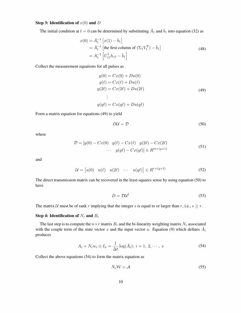
Step 3: Identification of x(0) and D
The initial condition at t = 0 can be determined by substituting A1 and b1 into equation (32) as
x(0) = A−11
[x(1)− b1
]= A−1
1
[the first column of (Σ1V
T1 )− b1
]= A−1
1
[U †1↑h1↑ − b1
] (48)
Collect the measurement equations for all pulses as
y(0) = Cx(0) +Du(0)
y(`) = Cx(`) +Du(`)
y(2`) = Cx(2`) +Du(2`)
...
y(q`) = Cx(q`) +Du(q`)
(49)
Form a matrix equation for equations (49) to yield
DU = D (50)
where
D = [y(0)− Cx(0) y(`)− Cx(`) y(2`)− Cx(2`)
· · · y(q`)− Cx(q`)] ∈ Rm×(q+1)(51)
and
U =[u(0) u(`) u(2`) · · · u(q`)
]∈ Rr×(q+1) (52)
The direct transmission matrix can be recovered in the least-squares sense by using equation (50) tohave
D = DU† (53)
The matrix U must be of rank r implying that the integer s is equal to or larger than r, i.e., s ≥ r.
Step 4: Identification of Nc and Bc
The last step is to compute the n×r matrixBc and the bi-linearity weighting matrixNc associatedwith the couple term of the state vector x and the input vector u. Equation (9) which defines Aiproduces
Ac +Ncwi ⊗ In =1
∆tlog(Ai); i = 1, 2, · · · , s (54)
Collect the above equations (54) to form the matrix equation as
NcW = A (55)
10

where
W = W ⊗ In ∈ Rrn×sn (56)
and
A =[
1∆t log(A1)−Ac 1
∆t log(A2)−Ac · · · 1∆t log(As)−Ac
]∈ Rn×sn (57)
So the bi-linearity matrix Nc can be solved by
Nc = AW† (58)
To determine the input matrixBc, first make the conversion from discrete-time to continuous-timeof equation (10) to yield
bci ≡[In∆t+
1
2!(Ac +Ncwi ⊗ In)(∆t)2 +
1
3!(Ac +Ncwi ⊗ In)2(∆t)3 + · · ·
]−1
bi (59)
where bi is computed from equation (47). From equations (6) and (10), form the matrix equationfor the continuous-time input matrix Bc as
BcW = B (60)
where
B =[bc1 bc2 · · · bcs
]∈ Rn×s (61)
The continuous-time input matrix Bc can then be obtained by solving
Bc = BW † (62)
To this end, we use the SEMP method to identify all continuous-time system matrices Ac, Bc,Nc, C and D together with the initial condition x(0) for the bilinear system described by equations(2) and (4). It is worth to mention that the SEMP method uses p+ 2 pulses of w1 and p+ 1 pulsesof w2, w3, . . . , ws. The order of these pulses is arbitrary such that one of the pulses denoted as w1 isused p+ 2 times to excite the bilinear system with free-decay response and the other wi’s are usedp+ 1 times each for continuous-time bilinear system identification.
BI-LINEARIZE PROCEDURE OF A NONLINEAR SYSTEM
The bi-linearization method used in this paper is so called the Carleman linearization. The Car-leman linearization technique is introduced first and an example of Euler’s equation for rigid bodyrotation is given later to illustrate this bi-linearization procedure.
11

Carleman linearization
The Carleman linearization method has been used for a class of nonlinear states equations of theform
x = f(x) +
r∑i=1
gi(x)ui
y = Cx, x(0) = 0
(63)
where x ∈ Rn is the state, u ∈ Rr is the input and ui is the ith entity of u, y ∈ Rm is themeasurement, f(x) ∈ Rn is a nonlinear function of the state, gi(x) is a nonlinear function of thestate which account for the influence of input ui, C ∈ Rm×n is a constant matrix. If f(x) and gi(x)in equation (63) are analytic in x, then it is called a linear-analytic state equation.23 Bilinear systemis an universal approximator for that kind of nonlinear system.33
Let the functions f(x) and gi(x) on the right hand side of equation (63) be expanded in terms ofpower series by
f(x) =N∑k=1
Fkx(k) + H.O.T
gi(x) =
N−1∑k=0
Gi,kx(k) + H.O.T
(64)
where the first N terms are explicitly retained, and
x(k) = x⊗ x⊗ · · · ⊗ x︸ ︷︷ ︸k−1 times
∈ Rnk
(65)
If H.O.T (high order terms) are neglected, substituting equation (64) into equation (63) yields
x =
N∑k=1
Fkx(k) +
N−1∑k=0
r∑i=1
Gi,kx(k)ui (66)
A differential equation of x(2) is developed by dropping the terms of degree greater than N
x(2) = x⊗ x+ x⊗ x
=
N∑k=1
Fkx(k) ⊗ x+
N−1∑k=0
r∑i=1
Gi,kx(k)ui ⊗ x+
x⊗N∑k=1
Fkx(k) + x⊗
N−1∑k=0
r∑i=1
Gi,kx(k)ui
=
N−1∑k=1
(Fk ⊗ In + In ⊗ Fk)x(k+1)+
N−2∑k=0
r∑i=1
(Gi,k ⊗ In + In ⊗Gi,k)x(k+1)ui; x(2)(0) = 0
(67)
12

where the last equality is based on the formula that (A⊗B)(C ⊗D) = AC ⊗BD.34
Continuing in this fashion yields the representation for x(j) to degree N of the form
x(j) =
N−j+1∑k=1
Fj,kx(j+k−1) +
N−j∑k=0
r∑i=1
Gi,j,kx(j+k−1)ui
x(j)(0) = 0, j = 1, 2, · · · , N
(68)
where Fj,k and Gi,j,k are defined by
F1,k =Fk ∈ Rn×nk
F2,k =Fk ⊗ In + In ⊗ Fk ∈ Rn2×nk+1
F3,k =Fk ⊗ In2 + In ⊗ Fk ⊗ In + In2 ⊗ Fk ∈ Rn3×nk+2
...
Fj,k =Fk ⊗ Inj−1 + In ⊗ Fk ⊗ Inj−2 + · · ·+ Inj−1 ⊗ Fk ∈ Rnj×nk+j−1
(69)
and
Gi,1,k =Gi,k ∈ Rn×nk
Gi,2,k =Gi,k ⊗ In + In ⊗Gi,k ∈ Rn2×nk+1
Gi,3,k =Gi,k ⊗ In2 + In ⊗Gi,k ⊗ In + In2 ⊗Gi,k ∈ Rn3×nk+2
...
Gi,j,k =Gi,k ⊗ Inj−1 + In ⊗Gi,k ⊗ Inj−2 + · · ·+ Inj−1 ⊗Gi,k ∈ Rnj×nk+j−1
(70)
Let us define an extended state x⊗ by
x⊗ =
x(1)
x(2)
...x(N)
∈ Rn⊗×1 (71)
where
n⊗ =
N if n = 1
n+ n2 + · · ·+ nN = nN+1−nn−1 otherwise
(72)
Collect equations (68) to form a bilinear state equation
x⊗ =Acx⊗ +Ncu⊗ x⊗ +Bcu (73)
13

where
Ac =
F1,1 F1,2 · · · F1,N
0 F2,1 · · · F2,N−1
0 0 · · · F3,N−2...
.... . .
...0 0 · · · FN,1
∈ Rn⊗×n⊗ ,
Gci =
Gi,1,1 Gi,1,2 · · · Gi,1,N−1 0Gi,2,0 Gi,2,1 · · · Gi,2,N−2 0
0 Gi,3,0 · · · Gi,3,N−3 0...
.... . .
......
0 0 · · · Gi,N,0 0
∈ Rn⊗×n⊗ ,
Nc =[Gc1 Gc2 · · · Gcr
]∈ Rn⊗×rn⊗ ,
Bc =
G1,1,0 G2,1,0 · · · Gr,1,0
0 0 · · · 0...
.... . .
...0 0 · · · 0
∈ Rn⊗×r
(74)
It should be noted that the definition of x⊗ in equation (71) produces redundancies. For example,if
x =[x1 x2
]T (75)
then
x(2) =[x2
1 x1x2 x2x1 x22
]T (76)
The redundancy can be eliminated by combining the repeated entries. The result is given by
x[2] =[x2
1 x1x2 x22
]T (77)
Accordingly, the columns of system matrices corresponding to all occurrences of the same stateshould be combined to a single column, and the extra rows should be eliminated. The number ofextended states constituted by x[·] , still denoted by n⊗, is re-calculated by24
n⊗ ≡min(n,N)∑i=1
(ni
)(Ni
)(78)
where(··
)is the binomial coefficient. In equation (77), the superscript bracket is used to denote
the difference from equations (76). But the parenthesis will be used instead for simplicity in thefollowing.
14

Example of Euler’s equation for rigid body rotation
Euler’s equation is commonly used for describing the rotation of a rigid body in a frame ofreference fixed in the rotating body
x = −J−1ΩJx+ J−1u (79)
where x ∈ R3 is the angular rate, J ∈ R3×3 is the moment of inertia, u ∈ R3 is the control input,and
Ω ≡
0 −x3 x2
x3 0 −x1
−x2 x1 0
(80)
From equations (73) and (74), a bilinear state equation can be derived by Carleman linearizationmethod to approximate Euler’s equation (79). Due to the special structure of Euler’s equation, Acis reduced to a block nilpotent matrix
Ac =
0 F1,2 0 · · · 00 0 F2,2 · · · 0...
......
. . ....
0 0 0 · · · FN−1,2
0 0 0 · · · 0
(81)
and Gci is reduced to a block lower off-diagonal form
Gci =
0 0 · · · 0 0
Gi,2,0 0 · · · 0 00 Gi,3,0 · · · 0 0...
.... . .
......
0 0 · · · Gi,N,0 0
(82)
Equations (81) and (82) clearly indicate that the system’s eigenvalues are all equal to zero, which, inturn, implies that the bilinearized version of Euler’s equation is also damping free like the originalnonlinear system.
Let J = diag[J1 J2 J3
]and
a1 = (J2 − J3)/J1
a2 = (J3 − J1)/J2
a3 = (J1 − J2)/J3
(83)
For N = 2, the state vector for the bilinear equation is
x⊗ =[x1 x2 x3 x2
1 x1x2 x1x3 x22 x2x3 x2
3
]T (84)
15

The corresponding system matrices shown in equations (74), (81) and (82) of the 9-state system(i.e., N = 2) are
F1,2 =
0 0 0 0 a1 00 0 a2 0 0 00 a3 0 0 0 0
,
G1,2,0 =
2/J1 0 00 1/J1 00 0 1/J1
0 0 00 0 00 0 0
, G2,2,0 =
0 0 01/J2 0 0
0 0 00 2/J2 00 0 1/J2
0 0 0
,
G3,2,0 =
0 0 00 0 0
1/J3 0 00 0 00 1/J3 00 0 2/J3
, Bc =
1/J1 0 00 1/J2 00 0 1/J3
0 0 00 0 00 0 00 0 00 0 00 0 0
(85)
Equation (85) will be used for the numerical example in the next section. For the higher orderof expansion, these matrices can be obtained by the same procedure, which is straightforward buttedious and will not be shown in this paper.
NUMERICAL RESULTS
Two nonlinear systems along with their corresponding bilinear systems are used to demonstratethe SEMP method in this section. The first example is a simple nonlinear system with a single state.The second example is Euler’s equation of three states for the rotation of a rigid body.
Simple Nonlinear System
The simple nonlinear system is given by
x = − sinx+ u
y = x, x(0) = 0(86)
After converting the nonlinear equation using Carleman linearization method and N = 3, the re-sulting equation is
x⊗ =
−1 0 1/60 −2 00 0 −3
x+
0 0 02 0 00 3 0
ux⊗ +
100
uy⊗ = x⊗
(87)
where
x⊗ =[x x2 x3
]T, x⊗(0) = 0 (88)
16

Let the identification parameters α = 5, β = 1, p = 9 (see equations (20) and (37)), the designedinput matrix is a scalar W = 2 (see equation (6)) for a single input system, and the samplingtime ∆t = 0.05sec. Here we assume that the three bilinear states are directly obtained by themeasurements, hence the minimum requirement for α can be reduced to 2 for a three-state andthree-measurement system. The quantity α = 2 satisfies the condition shown in equation (31), i.e.,αm ≥ n + m where n = 3 is the bilinear system order and m = 3 is the number of outputs. Theidentification results of the nonlinear system are shown in figures 2 and 3, The top part of figure 2shows the sampled (u1) and actual pulse (u) input to excite the simple nonlinear system, and thelower part gives the resulting measured output (y1) and the identified bilinear system output (y).The measured output is obtained from integrating the nonlinear system and reporting those valuesat sample points. Figure 3 shows the error history between the measured output and the identifiedbilinear system output. The quantities u1 and y1 are sampled input and output, while y1 is thesimulated output of the identified bilinear model excited by input sequence u1.
Next, let us compare the effect of the series expansion of order N . From equation (87), we knowthat the eigenvalues of Ac are −1, −2 and −3. Indeed, the eigenvalues are
[−1 −2 · · · −N
]if the order of expansion is N . Table 1 shows that the identified eigenvalues are close to the thoseof the actual bilinear model, and the errors are induced by the approximation. In other words, theoutput from the bilinear approximation does not match perfectly the actual output of the nonlinearsystem. The mean of the absolute value of the relative error, denoted by ye between the actualoutput of the nonlinear system and the simulated output of the identified bilinear system, decayswhen N ≤ 7 as expected, and maybe caused by the accuracy of computation, these values growinsignificantly from N = 7 to N = 9.
Table 1. Identification Results of Nonlinear System
N λ ye
1 [−0.9990] 1.1718e-0052 [−1.0006 −1.9956] 1.4385e-0063 [−1.0000 −2.0032 −2.9891] 3.4150e-0104 [−1.0000 −2.0000 −3.0085 −3.9790] 3.0466e-0115 [−1.0000 −2.0000 −3.0000 −4.0174 −4.9644] 1.5875e-0136 [−1.0000 −2.0000 −3.0000 −3.9998 −5.0312 −5.9442] 4.2539e-0147 [−1.0000 −2.0000 −3.0000 −4.0000 −4.9996 −6.0520 −6.9164] 2.7852e-0148 [−1.0000 −2.0000 −3.0000 −4.0000 −5.0001 −5.9989 −7.0830 −7.8774] 1.8127e-0139 [−1.0000 −2.0000 −3.0000 −4.0000 −5.0000 −6.0003 −6.9983 −8.1277 −8.8411] 3.9545e-013
The successful numerical experiment for this simple nonlinear system has verified Carleman’stheorem and the approximate relationship between bilinear system and linear-analytic nonlinearsystem.
Euler’s equation of rigid body rotation
Euler’s equation may be approximated by a bilinear system as shown in equations (73), (74),(81), (82) and (85) when the expansion order N = 2. Assume that the measurements are equal tothe states
y⊗ = x⊗ (89)
where the system order n⊗ = 9, 19, 34 obtained from equation (78) are corresponding to the expan-sion order N = 2, 3, 4, respectively.
17

Figure 2 Top plot shows the sample input (o) and the actual input pulse (-). Bottomplot shows the measured (o) and simulated (-) response.
Figure 3. Relative Error
18

Let us assumed that the moment of inertia shown in equation (79) is
J =
30 0 00 20 00 0 10
(90)
Because the number of measurements is equal to the number of states, one can set α = 2. Inaddition, let β = 1, the sampling time ∆t = 0.05 sec, and p = 34 to use the same input sequencefor cases N = 2, 3, 4. The input matrix is designed to be
W =
1 0 01 1 01 0 1
(91)
Figure 4 shows the three-input pulse sequence designed to excite the nonlinear system describedby Euler’s equation. The magnitude of the eigenvalues λ of the identified bilinear state matrixAc are compared in figure 5, which are closer to zero (the expected value) for larger N . Theidentification results of the nonlinear system using N = 2 are shown in figures 6, 7 and 8. Themeasured outputs are the state time histories obtained by integrating Euler’s equation, whereas thesimulated outputs are the state time histories computed from identified bilinear system equation.These figures show good agreement between measured and simulated outputs. The relative error (<1%) between the measured and simulated outputs of the identification results is displayed in figure 9.The largest relative error occur at about k = 300 for the second output which has smaller amplitudethan two other outputs. It clearly shows that the error histories grow with the increasing timesteps as expected due to the accumulated approximation error. Finally, figure 10 demonstrates thatthe higher-dimension approximation using Carleman linearization will produce better results closerto the real nonlinear system. However, higher-dimension approximation will introduce additionalnumerical errors that may exceed the reduction of the approximation errors. Further studies will betaken to address the problem of numerical errors for higher-dimension approximation.
CONCLUDING REMARKS
The improved single experiment with multiple pulses method is developed using a random per-mutation of input signals to excite all system modes. It improves the capability of the originalsingle experiment with multiple pulses method to a more general continuous-time bilinear systemidentification problem. The improved method was successfully used to identify bilinear models forapproximating nonlinear systems via the concept of Carleman linearization. Numerical examplesshow good agreements between the identified bilinear models and the original nonlinear systems.It demonstrates for the first time that a bilinear approximation of nonlinear systems can be possiblyidentified from experimental data.
REFERENCES[1] Juang, J. N., and Pappa, R. S., Effect of Noise on Modal Parameters Identified by the Eigensystem
Realization Algorithm, Journal of Guidance, Control, and Dynamics, Vol. 9, No. 3, May-June 1986,pp. 294-303.
[2] Juang, J. N., Cooper, J. E., and Wright, J. R., An Eigensystem Realization Algorithm Using DataCorrelations (ERA/DC) for Modal Parameter Identification, Journal of Control Theory and AdvancedTechnology, Vol. 4, No. 1, March 1988, pp. 5-14.
[3] Juang, J.-N., Phan, M., Horta, L. G., and Longman, R. W., ”Identification of Observer/Kalman FilterMarkov Parameters: Theory and Experiments,” Journal of Guidance, Control and Dynamics, Vol. 16,No. 2, Mar-Apr 1993, pp. 320-329
19

Figure 4. Sampled (o) and pulse (-) input sequence
Figure 5. Eigenvalues of identified Ac for Euler’s equation
20

Figure 6. Measured (o) and simulated (-) output y1 vs. y1
Figure 7. Measured (o) and simulated (-) output y2 vs. y2
21

Figure 8. Measured (o) and simulated (-) output y3 vs. y3
Figure 9. Relative error for N = 2
22

Figure 10. Relative error for N = 3
[4] Juang, J.-N., Applied System Identification, Prentice Hall, New Jersey, 1994.[5] Juang, J-N. and Phan, M. Q., Identification and Control of Mechanical Systems, Cambridge University
Press, New York, 2001.[6] Bruni, C., DiPillo, G., and Koch, G., On the Mathematical Models of Bilinear Systems, Ricerche Di
Automatica, 2 (1), 1971, pp. 11-26.[7] Bruni, C., DiPillo, G., and Koch, G., Bilinear Systems: An Appealing Class of Nearly Linear Systems
in Theory and Application, IEEE Transaction Automatic Control, AC-19, 1974, pp. 334-348.[8] Mohler, R. R., and Kolodziej, W. J., An Overview of Bilinear System Theory and Applications, IEEE
Transactions on Systems, Man and Cybernetics, SMC-10, 1980, pp. 683-688.[9] Elliott, D. L., Bilinear Systems, in Encyclopedia of Electrical Engineering, Vol. II John Webster (ed.),
John Wiley and Sons, New York, 1999, pp. 308-323.[10] Mohler, R. R., Nonlinear Systems: Vol. II, Applications to Bilinear Control, Prentice-Hall, New Jersey,
1991.[11] Paraskevopoulos, P., Tsirikos, A., and Arvanitis, K., A new orthogonal series approach to state space
analysis of bilinear systems, IEEE Transactions on Automatic Control, 39, 1994, pp. 793-797.[12] Karanam, V. R., Frick, P.A, and Mohler, R. R., Bilinear system identification by Walsh functions. IEEE
Transactions on Automatic Control, 23, 1973, pp. 709-713.[13] Jha, A. N., Saxena, A. S., and Rajamani, V. S., Parameter estimation algorithms for bilinear and non-
linear systems using Walsh functions: Recursive approach. International Journal of Systems Science23, 1992, pp. 283-290.
[14] Cheng, Bing and Ning-Show Hsu, Analysis and parameter estimation of bilinear systems via block-pulse functions. International Journal of Control, 36, 1982, pp. 53-65.
[15] Dai, Heping and Naresh K. Sinha, Robust identification of systems using block-pulse functions. IEEProceedings Part D: Control Theory and Applications, 139, 1992, pp. 308-316.
[16] Liu, C. C. and Shih, Y. P., Analysis and parameter estimation of bilinear systems via Chebyshev poly-nomials. Journal of the Franklin Institute, 317, 1984, pp. 373-382.
[17] Hwang, C. and Chen, M. Y., Analysis and parameter identification of bilinear systems via shiftedLegendre polynomials. International Journal of Control, 44, 1986, pp. 351-362.
23

[18] Daniel-Berhe, S. and Unbehauen, H., Bilinear continuous-time systems identification via Hartley-basedmodulating functions. Automatica 34, 1998, pp. 499-503.
[19] Daniel-Berhe, S. and Unbehauen H., State space identification of bilinear continuous-time canonicalsystems via batch scheme Hartley modulating functions approach. In Proceedings of the 37th IEEEConference on Decision and Control, Tampa, Florida, 1998(December), pp. 4482-4487.
[20] Karray, F. and Dwyer, T.A.W., III, On the nonlinear system identification of a class of bilinear dy-namical models, Proceedings of the 30th IEEE Conference on Decision and Control, 1991, vol.1 , pp.778-782.
[21] Karray, F.; Dwyer, T. and Makrakis, D., Bilinear approximation and identification for nonlinear systemmodeling, Proceedings of the 35th IEEE Conference on Decision and Control, 1996, vol.1, pp. 1088-1093.
[22] Kvaternik, R. G., and Silva, W. A., A Computational Procedure for Identifying Bilinear Representa-tions of Nonlinear Systems Using Volterra Kernels, NASA/TM-2008-215320, NASA Langley ResearchCenter, Hampton, Virginia, June 2008.
[23] Rugh, Wilson J., Nonlinear System Theory: The Volterra/Wiener Approach. Baltimore, Maryland: TheJohn Hopkins University Press. ISBN 0-8018-2549-0, 1981.
[24] Svoronos, Spyros, George Stephanopoulos and Rutherford Aris, Bilinear approximation of general non-linear dynamic systems with linear inputs. International Journal of Control 31(1), 1980, pp. 109-126.
[25] Lo, James Ting-Ho, Global Bilinearization of Systems with Control Appearing Linearly. SIAM J. Con-trol Volume 13, Issue 4, 1975, pp. 879-885.
[26] Juang, J.-N., Continuous-Time Bilinear System Identification, Nonlinear Dynamics, Kluwer AcademicPublishers, Special Issue 39(1-2), (January I-II 2005), pp. 79-94
[27] Sontag, E.D., Wang, Y., Megretski, A., Input Classes for Identification of Bilinear Systems, IEEETransactions on Automatic Control, 54, 2009, pp. 195-207.
[28] Majji, M., Juang, J.-N., and Junkins, J. L., Continuous-Time Bilinear System Identification Using Re-peated Experiments, the AAS/AIAA Astrodynamics Specialist Conference, Pittsburgh, Pennsylvania,August 9-13, 2009
[29] Juang, J.-N., Generalized Bilinear System Identification, The Journal of the Astronautical Sciences,January issue 2009.
[30] Aganovic, Z., and Gajic, Z. Linear Optimal Control of Bilinear Systems. Lecture Notes in Control andInformation Sciences, vol. 206. London: Springer-Verlag London Limited, 1995.
[31] Juang, Jer-Nan, Cheh-Han Lee and Shyh-Biau Jiang, Continuous-Time Bilinear System Identificationusing Single Experiment with Multiple Pulses, 20th AAS/AIAA Space Flight Mechanics Meeting, SanDiego, California, 2010, AAS 10-110.
[32] Isidori, Alberto and Antonio Ruberti, Realization theory of bilinear systems. In D. Q. Mayne and R.W. Brockett (Eds.), Geometric Methods in System Theory, pp. 83-130. Dordrecht, The Netherlands: D.Reidel Publishing Company. ISBN 90-277-0415-5, 1973.
[33] Mohler, Ronald R. and W. J. Kolodziej, An overview of bilinear system theory and applications. IEEETransactions on Systems, Man and Cybernetics 10(10), 1980, pp. 683-688.
[34] Brewer, John, Kronecker products and matrix calculus in system theory. IEEE Transactions on Circuitsand Systems, 25, 1978, pp.772-781.
24