Aalborg Universitet

ZigBee-based wireless sensor networks for classifying the behaviour of a herd ofanimals using classification treesNadimi, Esmaeil; Tangen Søgaard, Henning; Bak, Thomas

Published in:Biosystems Engineering

DOI (link to publication from Publisher):10.1016/j.biosystemseng.2008.03.003

Publication date:2008

Document VersionEarly version, also known as pre-print

Link to publication from Aalborg University

Citation for published version (APA):Nadimi, E., Tangen Søgaard, H., & Bak, T. (2008). ZigBee-based wireless sensor networks for classifying thebehaviour of a herd of animals using classification trees. Biosystems Engineering, 100(2), 167-176. DOI:10.1016/j.biosystemseng.2008.03.003

General rightsCopyright and moral rights for the publications made accessible in the public portal are retained by the authors and/or other copyright ownersand it is a condition of accessing publications that users recognise and abide by the legal requirements associated with these rights.

? Users may download and print one copy of any publication from the public portal for the purpose of private study or research. ? You may not further distribute the material or use it for any profit-making activity or commercial gain ? You may freely distribute the URL identifying the publication in the public portal ?

Take down policyIf you believe that this document breaches copyright please contact us at vbn@aub.aau.dk providing details, and we will remove access tothe work immediately and investigate your claim.

Downloaded from vbn.aau.dk on: May 01, 2017

Available at www.sciencedirect.com

journal homepage: www.elsevier.com/locate/issn/15375110

Research Paper: PA—Precision Agriculture

ZigBee-based wireless sensor networks for classifying thebehaviour of a herd of animals using classification trees

E.S. Nadimia,b,�, H.T. Søgaardc, T. Bakb

aFaculty of Engineering, Institute of Chemical Engineering, Biotechnology and Environmental Technology, University of Southern Denmark,

Niels Bohrs Alle 1, 5230 Odense, DenmarkbDepartment of Electronic Systems, Automatic and Control, Aalborg University, DenmarkcEngineering College of Arhus, Arhus, Denmark

a r t i c l e i n f o

Article history:

Received 28 September 2007

Accepted 10 March 2008

Available online 8 May 2008

An in-depth study of wireless sensor networks applied to the monitoring of animal

behaviour in the field is described. Herd motion data, such as the pitch angle of the neck

and movement velocity, were monitored by an MTS310 sensor board equipped with a 2-axis

accelerometer and received signal strength indicator functionality in a single-hop wireless

sensor network. Pitch angle measurements and velocity estimates were transmitted

through a wireless sensor network based on the ZigBee communication protocol. After data

filtering, the pitch angle measurements together with velocity estimates were used to

classify the animal behaviour into two classes; as activity and inactivity. Considering all the

advantages and drawbacks of classification trees compared to neural network and fuzzy

logic classifiers a general classification tree was preferred. The classification tree was

constructed based on the measurements of the pitch angle of the neck and movement

velocity of some animals in the herd and was used to predict the behaviour of other

animals in the herd. The results showed that there was a large improvement in the

classification accuracy if both the pitch angle of the neck and the velocity were employed as

predictors when compared to just pitch angle or just velocity employed as a single

predictor. The classification results showed the possibility of determining a general

decision rule which can classify the behaviour of each individual in a herd of animals. The

results were confirmed by manual registration and by GPS measurements.

& 2008 IAgrE. Published by Elsevier Ltd. All rights reserved.

1. Introduction

Animal behaviour monitoring represents a class of wireless

sensor network applications with enormous potential bene-

fits for practical farming. The knowledge of the herd

behaviour phases (activity, inactivity) can be monitored by

measuring relevant behaviour parameters. Such a behaviour

classification is potentially useful as a management tool in

grazing and production optimization. Furthermore, beha-

vioural monitoring would allow us to gain a better under-

standing of animal behaviour, detect individual animals with

potential health problems and generally optimize the grazing

process.

In order to monitor herd behaviour, data relevant to the

behaviour should be measured, aggregated, processed and

finally sent through a network to infrastructure facilities. In

ARTICLE IN PRESS

1537-5110/$ - see front matter & 2008 IAgrE. Published by Elsevier Ltd. All rights reserved.doi:10.1016/j.biosystemseng.2008.03.003

�Corresponding author at: Faculty of Engineering, Institute of Chemical Engineering, Biotechnology and Environmental Technology,University of Southern Denmark, Niels Bohrs Alle 1, 5230 Odense, Denmark.

E-mail addresses: esi@kbm.sdu.dk (E.S. Nadimi), hts@iha.dk (H.T. Søgaard), tba@es.aau.dk (T. Bak).

B I O S Y S T E M S E N G I N E E R I N G 1 0 0 ( 2 0 0 8 ) 1 6 7 – 1 7 6

animal science applications, the natural mobility of the herd

makes wireless sensor networks a good candidate for such

monitoring of animal behaviour parameters. Furthermore,

wireless sensor networks represent a significant advance over

traditional invasive methods of monitoring. The integration

of local processing and storage allows sensor nodes to

perform complex filtering and triggering functions, as well

as to apply application- or sensor-specific data compression

algorithms. Low-power radios with well-designed protocol

stacks allow generalized communications among network

nodes, rather than point-to-point telemetry. The computing

and networking capabilities allow sensor networks to be

reprogrammed or re-tasked after deployment in the field.

Therefore, monitoring animal behaviour parameters using

wireless sensor networks appears to provide a flexible and

robust monitoring system capable of remotely registering the

behaviour parameters which are of interest.

A herd of animals differs in many ways from man-made

systems of mobile robots because the behaviour of each

individual is governed by unpredictable natural instincts and

the environment into which it is placed (e.g. motion patterns

influenced by food sources and water). Therefore, by mon-

itoring a variety of behavioural parameters different aspects

of animal behaviour have been studied by different research-

ers. For instance, the positions of animals in the field were

tracked and monitored by White et al. (2001); Butler et al.

(2004); Zhang et al. (2004); Schwager et al. (2007); and Wark

et al. (2007) while Oudshoorn et al. (2008) investigated the

location and velocities of the movements in the field. The

different behaviour phases of dairy cows in a barn, such as

standing and lying down, were evaluated by Munksgaard

et al. (2005) and Wilson et al. (2005). However, none of these

studies used an online monitoring system based on wireless

sensor networks that classifies the behaviour of the animals

when they are in the field.

Behavioural parameters can be measured using different

types of sensors and consequently different strategies. GPS is

the most popular system employed in outdoor applications to

register position (Butler et al., 2004; Oudshoorn et al., 2008;

Schwager et al., 2007) but high energy consumption is one of

the main drawbacks of such a localization method. Further-

more, satellite connection loss in the areas of the field

covered by trees has been frequently reported by Oudshoorn

et al. (2008). This makes GPS less practical in terms of long-

term studies and less reliable for animal monitoring in some

specific environments.

Using an accelerometer attached to the leg of the animal

together with an offline data logger inside the barn was the

approach used by Munksgaard et al. (2005). They classified

cow behaviour into two phases, moving or stationary, while

Umstatter et al. (2006) used an offline pitch-roll sensor around

the neck of the animal. Sallvik and Oostra (2005) used video

processing combined with a radio frequency synchronization

unit (RFSU).

In this work, a wireless sensor network was established in

which ZigBee was implemented as the wireless communica-

tion protocol. Each node in the network was equipped with an

accelerometer in order to measure the pitch angle of the neck.

The nodes were programmed to measure received signal

strength (RSS) allowing the distance between wireless sensors

and a gateway to be estimated. Based on successive distance

estimates, the velocity could be estimated.

In order to fuse the measured behaviour parameters (i.e.

pitch angle of the neck and the movement velocity) and

consequently classify the animal behaviour into active or

inactive, different classification methods such as decision

trees, fuzzy logic and neural networks have been reported.

Comparing the advantages and disadvantages of decision

trees compared to fuzzy logic and neural network classifiers,

decision trees are the best candidate in terms of simplicity

and accuracy to evaluate the herd behaviour and as a result

they were employed here as the classification method.

The objectives of this paper were to classify the behaviour

of a herd of animals into two classes (active and inactive)

using the pitch angle measurements of the neck of the animal

together with the movement velocity estimates from a

wireless sensor network. A further objective was to solve a

specific problem regarding packet loss using data post-

processing.

2. Problem statement and background

2.1. Problem statement

In this paper, the problem of online and robust classification

of animal behaviour using a wireless sensor network has

been addressed. The main deficiencies were reported by

Umstatter et al. (2006), Nadimi et al. (2007) and Schwager et al.

(2007) and these were:

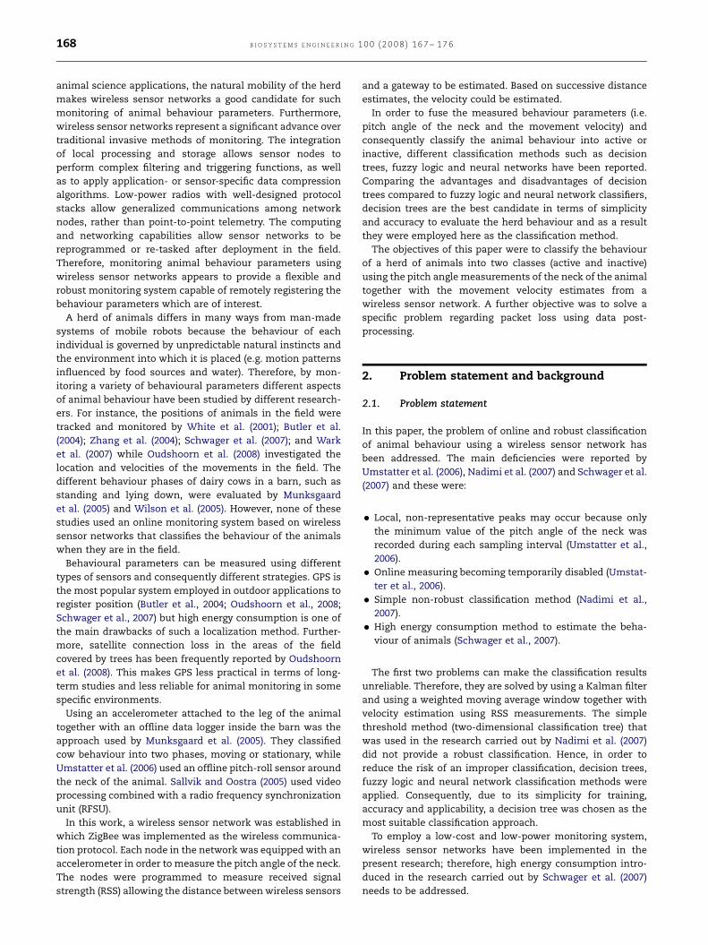
� Local, non-representative peaks may occur because only

the minimum value of the pitch angle of the neck was

recorded during each sampling interval (Umstatter et al.,

2006).

� Online measuring becoming temporarily disabled (Umstat-

ter et al., 2006).

� Simple non-robust classification method (Nadimi et al.,

2007).

� High energy consumption method to estimate the beha-

viour of animals (Schwager et al., 2007).

The first two problems can make the classification results

unreliable. Therefore, they are solved by using a Kalman filter

and using a weighted moving average window together with

velocity estimation using RSS measurements. The simple

threshold method (two-dimensional classification tree) that

was used in the research carried out by Nadimi et al. (2007)

did not provide a robust classification. Hence, in order to

reduce the risk of an improper classification, decision trees,

fuzzy logic and neural network classification methods were

applied. Consequently, due to its simplicity for training,

accuracy and applicability, a decision tree was chosen as the

most suitable classification approach.

To employ a low-cost and low-power monitoring system,

wireless sensor networks have been implemented in the

present research; therefore, high energy consumption intro-

duced in the research carried out by Schwager et al. (2007)

needs to be addressed.

ARTICLE IN PRESS

B I O S Y S T E M S E N G I N E E R I N G 1 0 0 ( 2 0 0 8 ) 1 6 7 – 1 7 6168

In order to address the problem of packet loss which

occasionally occurs in monitoring moving nodes in outdoor

environments when using wireless sensor networks, a

solution is proposed that predicts the lost states using a

Kalman filter.

2.2. Background

Location systems in outdoor environments have been a

research interest in the last few years. The methods for

locating a target in a geographical area based on the signal

received can be classified into three different groups.

2.2.1. Time of arrival (TOA) algorithmsThese algorithms determine the time a signal needs to travel

from a beacon to the target node. As distances in pasture

fields are not very large, the relative resolution acquired using

radio signals is very poor. However, other kinds of signals,

such as sound with shorter wavelengths, are easier to track

(Harter et al., 1999; Priyantha et al., 2000; Ward et al., 1997);

hence, radio interface may be used to synchronize the

network nodes and the sound signal to measure distances.

The precision of these methods is very good, but it requires

some additional hardware, in order to produce and detect the

sound signal.

2.2.2. Angle of arrival (AOA) algorithmsThese algorithms determine the direction that the arriving

signal comes from. Using the laws of trigonometry, the

position of the target node can be calculated (Arias et al.,

2004). The hardware needed may be quite complex, as it

requires either a mechanical system that moves the antenna

or an antenna array, whose radiation pattern can be altered

electronically.

2.2.3. Received signal strength (RSS) algorithmsIn order to obtain an accurate estimate of the distance

between nodes based on TOA and AOA algorithms, additional

localization hardware in terms of antennas or high-precision

clock synchronization is required. However, RSS algorithms

are based on the fact that a radio signal is attenuated with

increasing distance from the emitter. If the emitted power is

known, by measuring the incoming power at the receiver, the

distance between the transceiver and receiver can be

estimated. Nevertheless, the propagation medium exerts a

substantial influence on the arriving signal power; obstacles

attenuate the signal and produce reflections. Other signals or

even the reflections of the signal of interest may also interfere

with the emitted signal and alter the power measured (Arias

et al., 2004). In order to estimate the distance from RSS values,

range measurements should be carried out; i.e. estimating the

distance between two nodes given the signal strength

received by one node from the other. Signal strength

measurements are usually prone to inaccuracies and errors

and therefore calibration of such measurements is inevitable

before they can be used for localization. Thus, for this

algorithm to work, extensive preliminary field measurements

and calibrations are necessary.

3. Materials and methods

3.1. Materials

MPR2400 Micaz sensor motes from Crossbow were used for

the experiments in this paper. They have a Chipcon CC2420

radio, which uses a 2.4 GHz IEEE 802.15.4/ZigBee RF transcei-

ver with MAC support and provides a received signal strength

indicator (RSSI) output that is sampled by a 10-bit ADC. An

MTS310 sensor board equipped with a 2-axis accelerometer

and a temperature sensor was used to measure the pitch

angle of the neck of a cow. The temperature sensor was used

to calibrate the accelerometer readings as the digital

output of the accelerometer (duty cycle) can be varied by

temperature drifts. Consequently, to use the accelerometer as

a dual-axis tilt sensor to measure the pitch angle of the neck

of the cow, the raw accelerometer ADC readings were

converted to acceleration measurements (Analog device

dataste, 2007).

A TinyOS operating system was running on the motes (Gay

et al., 2007). The RSS data and the accelerometer readings

together with the temperature measurements were encapsu-

lated in the same packet. This designed packet structure

solves the problem reported by Nielsen et al. (2005) in

which two different packet structures were used to dissemi-

nate the data of RSS and acceleration. If each sensor

disseminates two kinds of packets, for instance one for RSS

and the other one for acceleration, losing one of them makes

the other packet useless. The selected sampling rate for the

packet dissemination was 1 Hz (Nadimi et al., 2008). Multiple

sensor nodes sent sensor readings to a base station or an

aggregation point in the network (gateway) using many to one

routing protocol.

The CC2420 radio supports up to 255 different transmission

power levels and allows for a programmable transmission

frequency. In order to minimize the number of variables in

the experiment, the RF transmission frequency and the

transition power were, respectively, fixed at a single fre-

quency band (2.48 GHz) and at the maximum transmission

power (1 mW).

The case study in this experiment was a group of dairy

cows. The experiment was carried out for 3 days with 4 cows

6 h per day as an average. Each cow was equipped with a

wireless node and a GPS as a reference around the neck

(Fig. 1). During the calibration process, the nodes were placed

at fixed distances (1–30 m far from the gateway) for 5 min at

each distance. The sampling time was set to 1 s and it was

expected to receive 300 samples per distance. As without any

energy budgeting, MPR2400 Micaz nodes operating at 100%

duty cycle can approximately operate for 7 days (Polastre,

2003), normal alkaline AA batteries with a conservative

estimate of 2200 mAh total capacity were utilised which

provided enough power for each sensor node during the

whole experiment (3 days).

The shape of the field was rectangular (80�40 m2). Each

day, a new field with new grass was provided for the cows.

The gateway was installed in the middle of one of the longest

sides. Manual registration of the behaviour was also carried

out.

ARTICLE IN PRESS

B I O S Y S T E M S E N G I N E E R I N G 1 0 0 ( 2 0 0 8 ) 1 6 7 – 1 7 6 169

3.2. Methods

3.2.1. RSS and acceleration measurements filteringWhen data travel along unreliable communication channels

in a large wireless sensor network, the effect of communica-

tion delays and loss of information cannot be neglected. This

problem was addressed here by using separate discrete

Kalman filters for RSS and acceleration observations where

the arrival of observation packets was modelled as a random

process. The statistical convergence properties of the state

error covariance were studied, showing the existence of a

critical value for the arrival probability of the observations,

beyond which a transition to an unbounded state error

covariance occurs. Due to high rate energy absorption in

outdoor applications, packets either arrive or are lost within a

sampling period following a Bernoulli process with parameter

0o 1(packet arrival probability). A Kalman Filter, however,

still provides estimates in case of intermittent observations

(Sinopoli et al., 2004). With these assumptions, the Kalman

filter equations for scalar states and measurements were as

follows:

� Time update equations:

x̂�kþ1 ¼ jkx̂k (1)

P�kþ1 ¼ jkPkjTk þ Qk (2)

� Observation update equations

Pk ¼ ð1� gkKkHkÞP�k (3)

x̂k ¼ x̂�k þ gkKkðzk � Hkx̂�k Þ (4)

Kk ¼ P�k HTk ðHkP�k HT

k þ RkÞ�1 (5)

where k ¼ 0,1,2,y is the time instant and x̂�k and x̂k are a

priori and a posteriori state estimates which could either be

RSS or acceleration. Pk� and Pk are a priori and a posteriori

estimates of error variance, and Kk is the Kalman gain. Qk is

the process noise covariance, Rk the measurement noise

covariance and gk is the arrival sequence which is common

for the RSS filter and the acceleration filter and is modelled by

a Bernoulli process (1 if arrived; 0 if lost). The underlying

process (pitch angle of the neck and the movement velocity)

has been assumed to be a discrete time Wiener process

described by Eqs. (6) and (7) in the state-space form

xkþ1 ¼ jkxk þwk (6)

zk ¼ Hkxk þ vk (7)

where xk is the true (unknown) state, zk is the RSS measure-

ment or acceleration measurement if the packet arrives, wk 2

Nð0;QkÞ is the process noise and vk 2 Nð0;RkÞ is the measure-

ment noise (wk and vk are independent). Hk and jk are set to 1

independently of time (k). To estimate the states, separate

scalar filters for RSS and acceleration were employed. As the

Kalman filter was designed to handle intermittent observa-

tions, it estimated the states not observed due to the packet

loss and thereby reduced the effect of measurement noise.

The existence of a critical value lc for the arrival probability

of the observation update has been shown by Sinopoli et al.

(2004), such that for l4lc, the mean state covariance E[Pk] is

bounded for all initial conditions and for lplc the mean state

covariance diverges for some initial condition. A lower bound

l and upper bound l can be found for the critical probability

lc, i.e, lplcpl. The lower bound can be expressed in closed

form while the upper bound is the solution of a linear matrix

inequality (LMI). In some special cases when Hk is invertible or

jk has a single unstable eigenvalue, the two bounds coincide,

giving a tight estimate. Since Hk is set to 1, the critical arrival

probability can be expressed as (Sinopoli et al., 2004):

lc ¼ 1�1p2

p ¼maxðeigðjkÞÞ (8)

As the average value of l was 0.7 in the present study and

lc ¼ 0 for a discrete time Wiener process, the inequality l4lc

was fulfilled.

During the grazing period, the head moves upwards with

certain intervals making the pitch angle readings close to zero

during very short time periods (Umstatter et al., 2006). To

avoid classifying these events as a part of an inactivity phase,

the Kalman filtered data were further filtered using a

weighted moving average window. In order to select an

appropriate window, the properties of different common

windows such as rectangular, Bartlett, Hanning, Hamming,

Blackman and Kaiser windows have been considered. The

two main criteria to measure the performance of different

windows are (Ashan, 2003):

� Reduction of smearing or spectral resolution improvement

which can be achieved by reducing the main lobe width in

the frequency domain.

� Reduction of leakage or amplitude resolution improvement

which can be achieved by side lobe reduction.

The first property is the ability of the filter to separate

signals whose frequencies are nearly the same while the

second property is the capability of separating unequal

ARTICLE IN PRESS

Node

GPS

Y

X

Fig. 1 – Wireless node and GPS around the neck.

B I O S Y S T E M S E N G I N E E R I N G 1 0 0 ( 2 0 0 8 ) 1 6 7 – 1 7 6170

amplitudes in order to prevent the low-amplitude peaks from

being swamped by leakage from the higher amplitude peaks.

To fulfil the criteria, knowledge of the narrow main lobe width

and low side lobe amplitude is required. While these two

conditions cannot be met simultaneously, the trade-off

between the main lobe width and the side lobe amplitudes

can be quantified by a Kaiser window represented by

(Oppenheim et al., 1999):

Wn ¼

I0 paffiffiffiffiffiffiffiffiffiffiffiffiffiffiffiffiffiffiffiffiffiffiffiffi1�ðð2n=NÞ�1Þ2p� �

I0ðpaÞif 0pnpN

0 otherwise

8<: (9)

where I0( � ) is the zero-order modified Bessel function of the

first kind. The real parameter a which determines the shape

of the window is set to 0.5 and the integer N gives the length

of the window (N+1 points). The window length was chosen

less than the length of typical inactive periods to be sure that

these periods would be detected (N ¼ 1000, i.e. 0.278 h).

3.2.2. Acceleration measurements analysisDuring the active period, the animals are grazing or searching

for grass with their necks down and their movement

velocities are non-zero. In the inactive phase, the necks are

almost horizontal and their movement velocities are zero.

Therefore, measuring the pitch angle of the neck together

with the movement velocity was chosen as the basis for the

behaviour classification.

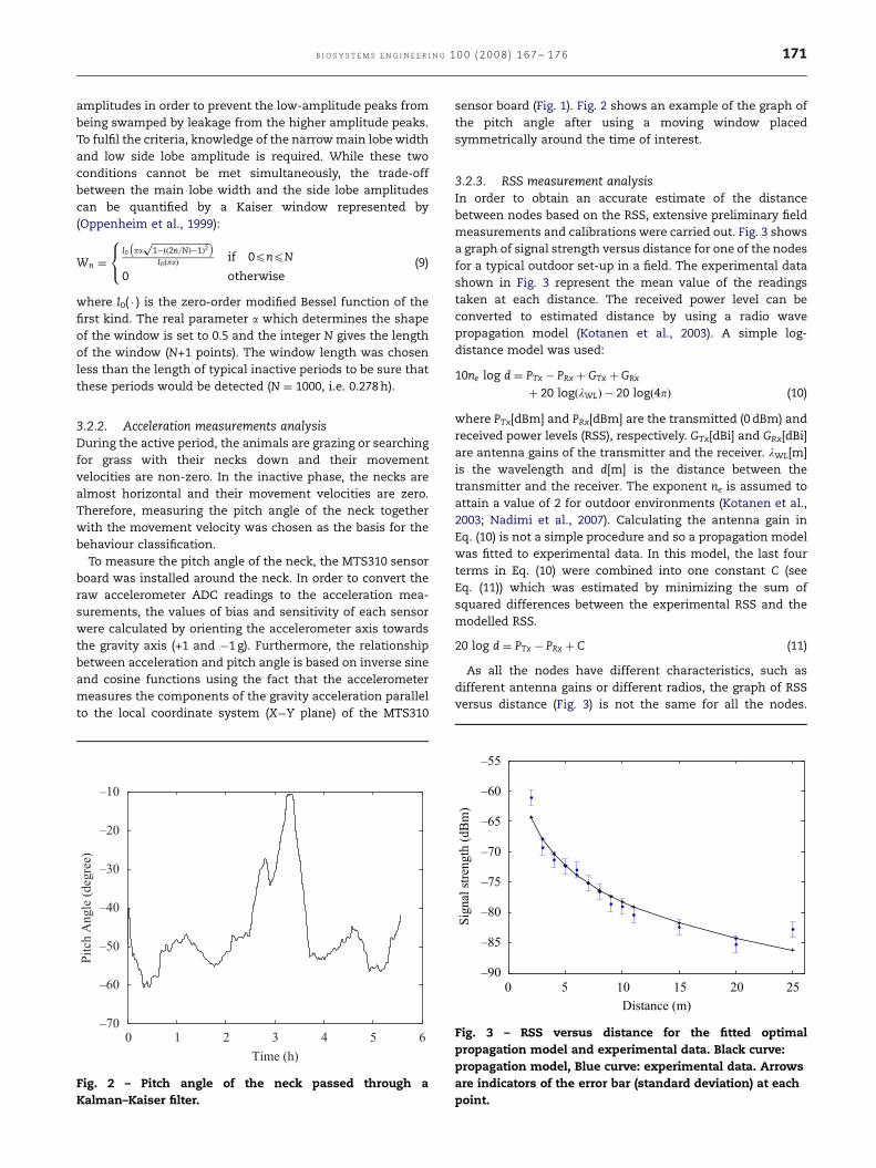
To measure the pitch angle of the neck, the MTS310 sensor

board was installed around the neck. In order to convert the

raw accelerometer ADC readings to the acceleration mea-

surements, the values of bias and sensitivity of each sensor

were calculated by orienting the accelerometer axis towards

the gravity axis (+1 and �1 g). Furthermore, the relationship

between acceleration and pitch angle is based on inverse sine

and cosine functions using the fact that the accelerometer

measures the components of the gravity acceleration parallel

to the local coordinate system (X�Y plane) of the MTS310

sensor board (Fig. 1). Fig. 2 shows an example of the graph of

the pitch angle after using a moving window placed

symmetrically around the time of interest.

3.2.3. RSS measurement analysisIn order to obtain an accurate estimate of the distance

between nodes based on the RSS, extensive preliminary field

measurements and calibrations were carried out. Fig. 3 shows

a graph of signal strength versus distance for one of the nodes

for a typical outdoor set-up in a field. The experimental data

shown in Fig. 3 represent the mean value of the readings

taken at each distance. The received power level can be

converted to estimated distance by using a radio wave

propagation model (Kotanen et al., 2003). A simple log-

distance model was used:

10ne log d ¼ PTx � PRx þ GTx þ GRx

þ 20 logðlWLÞ � 20 logð4pÞ (10)

where PTx[dBm] and PRx[dBm] are the transmitted (0 dBm) and

received power levels (RSS), respectively. GTx[dBi] and GRx[dBi]

are antenna gains of the transmitter and the receiver. lWL[m]

is the wavelength and d[m] is the distance between the

transmitter and the receiver. The exponent ne is assumed to

attain a value of 2 for outdoor environments (Kotanen et al.,

2003; Nadimi et al., 2007). Calculating the antenna gain in

Eq. (10) is not a simple procedure and so a propagation model

was fitted to experimental data. In this model, the last four

terms in Eq. (10) were combined into one constant C (see

Eq. (11)) which was estimated by minimizing the sum of

squared differences between the experimental RSS and the

modelled RSS.

20 log d ¼ PTx � PRx þ C (11)

As all the nodes have different characteristics, such as

different antenna gains or different radios, the graph of RSS

versus distance (Fig. 3) is not the same for all the nodes.

ARTICLE IN PRESS

0 1 2 3 4 5 6–70

–60

–50

–40

–30

–20

–10

Time (h)

Pitc

h A

ngle

(deg

ree)

Fig. 2 – Pitch angle of the neck passed through a

Kalman–Kaiser filter.

0 5 10 15 20 25–90

–85

–80

–75

–70

–65

–60

–55

Distance (m)

Sign

al st

reng

th (d

Bm

)

Fig. 3 – RSS versus distance for the fitted optimal

propagation model and experimental data. Black curve:

propagation model, Blue curve: experimental data. Arrows

are indicators of the error bar (standard deviation) at each

point.

B I O S Y S T E M S E N G I N E E R I N G 1 0 0 ( 2 0 0 8 ) 1 6 7 – 1 7 6 171

Therefore, the optimal constant C in Eq. (11) differed from one

node to another one (the range varied between �60 and

�55 dBm). In the present research, the constant C calculated

for one of the nodes (�56 dBm) was selected as the optimal

constant representing antenna gain and wavelength effect for

all the nodes. This strategy tends to reduce the precision of

the results of each individual node (curve fit and estimated

distance between the nodes and the gateway) and conse-

quently the whole system. However, this is a practical

solution for monitoring a large herd of animals with a large

number of nodes as estimating the optimal constant C for all

the nodes could be a time- and energy-consuming process.

Using Eq. (11), the distance dk between the cow node and

the gateway was estimated for each time instant k, and the

change in distance during each sampling interval could be

estimated as Dk ¼ |dk�dk�1|. This distance change was taken

as a rough estimate of the distances walked by the cow during

the sampling interval. An example of estimated distances

walked per sampling interval (velocity) versus time is shown

in Fig. 4. A comparison between estimated and true distance

walked during one sampling interval (displacement) is

illustrated in Fig. 5.

With the methodology used in this research to estimate the

velocity using RSS, if an animal walks in a circle around the

gateway, the velocity will be estimated as zero. However, it

should be noted that in practice this rarely happens; as

animal behaviour studies have demonstrated, cows’ walking

patterns are usually linear (Oudshoorn et al. 2008). To confirm

the visual observation that cows rarely move on a circle, the

position of cows in the field was registered by GPS and was

sampled every 60 s (Fig. 6). Based on GPS registrations and the

equations of semicircles (see Fig. 6), it was demonstrated that

three consecutive locations were not on a same circle. This

drawback of the method would only become relevant with a

large field where the semicircles far from the gateway turn

into straight lines. In this experiment the size of the field was

chosen as 40�80 m2 and therefore the radius of the largest

semicircle was 40 m.

In order to verify the estimated distance using the RSS, a

GPS (Fig. 1) was employed to measure the position and the

distance of wireless nodes from the gateway. Fig. 7(a) shows

the measured distance by GPS between one of the nodes and

the gateway versus the distance estimated by the RSS

approach. Fig. 7(b) presents the distance of a node from the

gateway measured by GPS and estimated by RSS measure-

ments versus time. The distance between the nodes and the

gateway using RSS was overestimated when compared to the

distance determined by GPS, as can be seen from the curve

fitted to the data in Fig. 7, because the fitted propagation

model (Eq. (11)) overestimated the distance as a total. In

contrast to distance, the estimated walked distance using the

RSS algorithm underestimated the measured GPS displace-

ment as shown in Fig. 5.

ARTICLE IN PRESS

0 1 2 3 4 5 60

0.05

0.1

0.15

0.2

0.25

0.3

Time (h)

Estim

ated

dis

tanc

e w

alke

d pe

r sam

plin

g tim

e (m

)

Fig. 4 – Estimated distance walked per sampling interval.

Gateway Position before moving

Position after moving

dk–1

dk

Dk

�xk

Fig. 5 – Distance walked during one sampling interval as

estimated from RSS measurements (Dk) and based on true

positions (Dxk).

0 10 20 30 40 50 60 700

5

10

15

20

25

30

35

40

45

Shor

t sid

e of

the

fenc

e (m

)

GatewayLong side of the fence (m)

Fig. 6 – Registered position of cows’ movement in the field

(black ) and half circles centred on the gateway (blue

curves).

B I O S Y S T E M S E N G I N E E R I N G 1 0 0 ( 2 0 0 8 ) 1 6 7 – 1 7 6172

3.2.4. Behaviour classification based on classification treesWith non-linear least squares fitting and other parametric

approaches, it is assumed that the relationship between the

response and the predictor is known or can be identified

based on the data. Assuming, instead, that the relationship is

unknown and there is no need to identify a specific relation-

ship, a non-parametric regression fitting approach can be

applied.

One such approach is based on trees (Breiman, 1998).

Classification trees are used to predict the membership of

cases or objects in classes of a categorical dependent variable

from measurements of one or more predictor variables. The

goal of classification trees is to predict or explain responses of

a categorical dependent variable. The flexibility of classifica-

tion trees makes them a very attractive analysis option.

Classification trees use a ‘‘white box’’ decision rule if a given

result is provided by a model and the explanation for the

result is easily replicated by simple mathematics, while an

artificial neural network or a fuzzy logic classifier uses a

‘‘black box’’ model in which the explanation for the results

can be excessively complex for a decision maker to compre-

hend. Another drawback of a neural network or a fuzzy

classifier is the slow process of training (Schetinin et al., 2004).

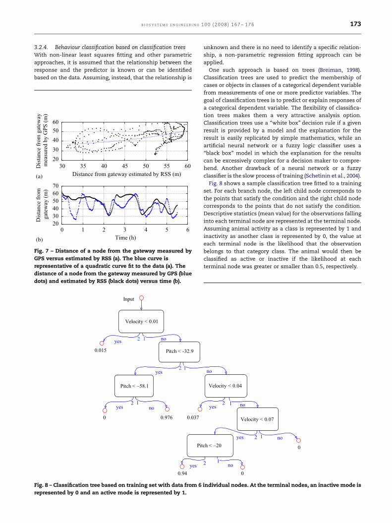
Fig. 8 shows a sample classification tree fitted to a training

set. For each branch node, the left child node corresponds to

the points that satisfy the condition and the right child node

corresponds to the points that do not satisfy the condition.

Descriptive statistics (mean value) for the observations falling

into each terminal node are represented at the terminal node.

Assuming animal activity as a class is represented by 1 and

inactivity as another class is represented by 0, the value at

each terminal node is the likelihood that the observation

belongs to that category class. The animal would then be

classified as active or inactive if the likelihood at each

terminal node was greater or smaller than 0.5, respectively.

ARTICLE IN PRESS

30 35 40 45 50 55 602030405060

Distance from gateway estimated by RSS (m)

0 1 2 3 4 5 6203040506070

Time (h)

Dis

tanc

e fr

om g

atew

ay (m

)

Dis

tanc

e fr

om g

atew

ay

mea

sure

d by

GPS

(m)

Fig. 7 – Distance of a node from the gateway measured by

GPS versus estimated by RSS (a). The blue curve is

representative of a quadratic curve fit to the data (a). The

distance of a node from the gateway measured by GPS (blue

dots) and estimated by RSS (black dots) versus time (b).

Velocity < 0.01

Pitch < -32.9

Pitch < –58.1 Velocity < 0.04

Velocity < 0.07

Pitch < –20

0.015

0 0.976 0.037

0

00.94

Input

noyes

noyes

noyes yes no

yes no

yes no

2

2 1

2

2

22

1

1

11

1

Fig. 8 – Classification tree based on training set with data from 6 individual nodes. At the terminal nodes, an inactive mode is

represented by 0 and an active mode is represented by 1.

B I O S Y S T E M S E N G I N E E R I N G 1 0 0 ( 2 0 0 8 ) 1 6 7 – 1 7 6 173

The training sets and the validation sets were chosen

random among all the registered data sets. The training set

was constructed by predictors (velocity, pitch angle) and

responses (behaviour phase). The data of predictors were

registered by individual wireless nodes in which each node

was associated with an animal and the responses were

registered manually. The main purpose of the classification

method presented in this paper is to construct a general tree

which could predict the behaviour of the animals in the

training set as well as animals in the validation set. The

validation set was chosen as the data set of registered

behaviour of animals which were not involved in the training

set.

A tree as exemplified by Fig. 8 having many branches may

overfit the training set and introduces uncertainties regarding

prediction of new unseen data. Some of the lower branches

may be strongly affected by outliers and other artefacts of the

training set, and therefore the discrimination between some

of the predictors would be less than the resolution. It would

be preferable to find a simpler tree that avoids this problem of

overfitting.

Pruning is basically an estimation problem in which the

best tree size is estimated based on the error cost. Accuracy is

computed by counting the misclassifications at all tree nodes.

Then, the tree is pruned by computing the estimates

following the bottom–up approach (post-pruning). The re-

substitution estimate of the error variance for this tree and a

sequence of simpler trees are then computed. Because this

probably underestimates the true error variance, the cross-

validation estimation is computed next. The cross-validation

estimate provides an estimate of the pruning level needed to

achieve the best tree size. Finally, the best tree is the one that

has a residual variance no more than one standard error

above the minimum values along the cross-validation line

(Fig. 9).

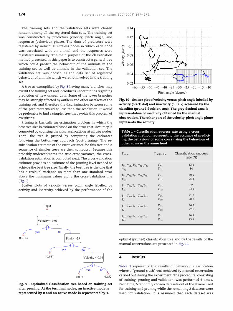
Scatter plots of velocity versus pitch angle labelled by

activity and inactivity achieved by the performance of the

optimal (pruned) classification tree and by the results of the

manual observations are presented in Fig. 10.

4. Results

Table 1 represents the results of behaviour classification

where a ‘‘ground-truth’’ was achieved by manual observation

carried out during the experiment. The procedure, consisting

of training, pruning and validation, was performed 6 times.

Each time, 6 randomly chosen datasets out of the 8 were used

for training and pruning while the remaining 2 datasets were

used for validation. It is assumed that each dataset was

ARTICLE IN PRESS

0.0143 Pitch < -33

Velocity < 0.040.957

0.037 0.652

Input

Velocity < 0.01

yes no

noyes

noyes

2

2

2

1

1

1

Fig. 9 – Optimized classification tree based on training set

after pruning. At the terminal nodes, an inactive mode is

represented by 0 and an active mode is represented by 1.

–60

0.14

–55 –50 –45 –40 –35 –30 –25 –20 –15 –10

0.12

0.1

0.08

0.06

0.04

0.02

Pitch angle (degree)

Velo

city

(ms–1

)

Fig. 10 – Scatter plot of velocity versus pitch angle labelled by

activity (black dot) and inactivity (blue * ) achieved by the

classifier (pruned decision tree). The grey dashed area is

representative of inactivity obtained by the manual

observation. The other part of the velocity-pitch angle plane

represents the activity.

Table 1 – Classification success rate using a crossvalidation method, representing the accuracy of predict-ing the behaviour of some cows using the behaviour ofother cows in the same herd

Ttrain Tvalidation Classification successrate (%)

T11, T21, T31, T12 ,T22

,T42

T041 83.2

T032 80

T11 ,T21, T31, T22, T32,

T42

T041 80.5

T012 95.1

T11, T21, T41, T22, T32,

T42

T031 82

T012 93.4

T11, T31, T41, T12, T32,

T42

T021 71.8

T022 70.2

T21, T31, T41, T12, T32,

T42

T011 84.3

T022 72.6

T21, T31, T41, T22, T32,

T42

T011 90.3

T012 95.5

B I O S Y S T E M S E N G I N E E R I N G 1 0 0 ( 2 0 0 8 ) 1 6 7 – 1 7 6174

associated with an animal; therefore, the dataset associated

with cow a( ¼ 1,2,3,4)in day q( ¼ 1,2) was defined as Taq or T0aq

in case that dataset was used in the training set or in the

validation set, respectively.

The measurements of pitch angle and velocity were used as

predictors and the behaviour classified as activity or inactivity

was used as the response. It can be concluded from the table

that a general classification tree, as shown in Fig. 9

constructed by the data from a subset of cows, could predict

the behaviour of other cows with a high classification success

rate. Similar classification tables have been achieved by only

considering the pitch angle or velocity as the predictor but the

classification results showed much lower success rates

compared to the results of Table 1. Constructing the tree only

based on pitch angle measurements as the predictor showed

that the classification tree could predict the behaviour with a

55% success rate while the velocity as the unique predictor

could classify the behaviour with 43% accuracy on average.

Based on manual registration and GPS measurements,

cow2 associated with node2 was the most active cow (92%

of time active) in the group. It can be seen in Table 1 that the

classification success rate is minimum when the data of cow2

are not considered for training the tree. On the other hand,

cow1 was the most inactive animal in the group (active 83% of

time) and hence had a limited effect on training the tree.

As the evaluation criterion most used for a classifier is the

error rate (the ratio of the number of falsely classified samples

to the whole number of samples), this rate has been

calculated for the pruned decision tree shown by Fig. 9, a

trained fuzzy logic classifier and a trained neural network

classifier. Furthermore, the classification cost in terms of

number of nodes or neurons was also taken into account.

While a simple classification tree with 4 terminal nodes

could classify the behaviour with an average error rate of

16.76%, the same data sets were imported to the fuzzy logic

classifier and an error rate of 19.32% was achieved by 70

trained epochs and in the case of a linear neural network

classifier, an error rate of 18.65% was achieved by 100

neurons.

5. Conclusions

Pitch angle measurements as well as movement velocity

estimates were successfully transmitted through a wireless

sensor network and used to classify the animal behaviour

into two classes as active and inactive. The proposed Kalman

filter could handle the problem raised by packet loss due to

intermittent observation by estimating the lost states. The

problem of non-representative local peaks due to head

movements during the grazing period was addressed and

robustly solved using a Kaiser window. Classification trees

showed advantages over neural network and fuzzy logic

classifiers and therefore a general classification tree was

preferred. The classification tree was constructed based on

the measurements of pitch angle of the neck and the

movement velocity. The results showed that there was a

large improvement in the classification accuracy if both the

pitch angle of the neck and the velocity were employed as

predictors in comparison to just pitch angle or just velocity

employed as a single predictor. The results suggested that a

classification tree for behaviour comprised of active and less

active cows. In spite of this, it appeared that a success rate of

at least 70.2% could be achieved. The results have been

confirmed by manual registration and by GPS measurements.

To confirm or reject this percentage, a study including more

cows observed during more days is necessary. The classifica-

tion results proved the possibility of determining a general

decision rule (model) which can classify the behaviour of each

individual in a herd of animals. Consequently, the behaviour-

al model could then be used for purposes such as behaviour

control. The classification results showed an improve-

ment compared to the results achieved by other studies;

some key challenges such as a more robust wireless sensor

network, with less percentage of packet loss, and more

precise methods to estimate the movement velocity are

required.

R E F E R E N C E

Analog device dataste (2007). ADXL202JE Accelerometer DataSheet

Arias J; Zuloaga A; Lazaro J; Andreu J; Astarloa A (2004). Malguki:an RSSI based ad hoc location algorithm. Journal of Micro-processors and Microsystems, 28, 403–409

Ashan S T (2003). Optimal window design. Journal of IEEEPotentials, 21(5), 39–43

Breiman L (1998). Classification and Regression Tree. Chapman &Hall/CRC, Boca Raton, FL

Butler Z; Corke P; Peterson R; Rus D (2004). Networked cows:virtual fences for controlling cows. International Conferenceon Robotics and Automation (ICRA)

Gay D; Levis P; Culler D (2007). Software design patterns forTinyOS. ACM Transactions on Embedded Computing Systems(TECS), 6(4)

Harter A; Hopper A; Steggles P; Ward A; Webster P (1999). Theanatomy of a context-aware application. Mobile Computingand Networking, 59–68

Kotanen A; Hannikainen M; Leppakoski H; Hamalainen T D(2003). Experiment on local positioning with Bluetooth.information technology: coding and computing [computersand communications]. Proceedings of the ITCC 2003 Interna-tional Conference, pp 297–303.

Munksgaard L; Jensen M B; Herskin M S; Levendahl P (2005). Theneed for lying time in high producing dairy cows. Proceedingsof the 39th International Congress of the ISAE, Vol. 38,Kanagawa, Japan.

Nadimi E S; Søgaard H T; Bak T; Oudshoorn F W (2008).ZigBee-based wireless sensor networks for monitoring ani-mal presence and pasture time in a strip of new grass.Journal of Computers and Electronics in Agriculture, 61(2),79–87

Nadimi E S; Søgaard H T; Oudshoorn F W; Blanes-Vidal V; Bak T(2007). Monitoring cow behaviour parameters based onreceived signal strength using wireless sensor networks. ThirdEuropean Conference on Precision Livestock Farming. Greece

Nielsen C; Kracht S; Svenstrup M (2005). Localization usingreceived signal strength indicator. Report, Aalborg University

Oppenheim A V; Schafer R W; Buck J R (1999). Discrete-time SignalProcessing. Prentice-Hall, Upper Saddle River, NJ

Oudshoorn F; Kristensen T; Nadimi E S (2008). Dairy cowdefecation and urination frequency and spatial distributionrelated to time limited grazing. Journal of Livestock ProductionSciences, 113(1), 62–73

ARTICLE IN PRESS

B I O S Y S T E M S E N G I N E E R I N G 1 0 0 ( 2 0 0 8 ) 1 6 7 – 1 7 6 175

Polastre J (2003). Design and implementation of wireless sensornetworks for habitat monitoring. Master’s Thesis, Universityof California, Berkeley

Priyantha N B; Chakraborty A; Balakrishnan H (2000). The cricketlocation-support system. Mobile Computing and Networking,32–43

Sallvik K; Oostra H H (2005). Automatic Identification andDetermination of the Location of Dairy Cows, PrecisionLivestock Farming ‘05 (Cox S, ed.)

Schetinin V; Fieldsend J E; Partridge D; Krzanowski W J; Everson RM; Bailey T C; Hernandez A (2004). The Bayesian decision treetechnique with a sweeping strategy. International Conferenceon Advances in Intelligent Systems—Theory and Applications,Centre de Recherche Public Henri Tudor, Luxembourg-Kirch-berg, Luxembourg, November 2004

Schwager M; Anderson M D; Butler Z; Rus D (2007). Robustclassification of animal tracking data. Computers and Elec-tronics in Agriculture, 56(1), 46–59

Sinopoli B; Schenato L; Franceschetti M; Poolla K; Jordan M I;Sastry S S (2004). Kalman filtering with intermittent observa-tion. IEEE Transaction on Automatic Control, 9, 1453–1464

Umstatter C; Waterhouse A; Holland J (2006). An automatedmethod of simple behaviour classification as a tool for

management improvement in extensive systems. FourthInternational Workshop on Smart Sensors in LivestockMonitoring. Book of Abstracts, pp 57–58

Ward A; Jones A; Hopper A (1997). A new location techniquefor the active office. IEEE Personal Communications,42–47

Wark T; Crossman C; Hu W; Guo Y; Valencia P; Sikka P; Corke P;Lee C; Henshall J; Prayaga K; O’Grady J; Reed M; Fisher A(2007). The design and evaluation of a mobile sensor/actuatornetwork for autonomous animal control. Proceedings of thesixth International Conference on Information Processing inSensor Networks, pp 206–215 978-1-59593-638

White S L; Sheffield R E; Washburn S P; King L D; Green J T (2001).Spatial and time distribution of dairy cattle excreta in anintensive pasture system. Journal of Environmental Quality,30(November–December)

Wilson S C; Dobos R C; Fell L R (2005). Spectral analysis of feedingbehaviour of cattle kept under different feedlot conditions.Journal of Applied Animal Welfare Science

Zhang P; Sadler C M; Lyon A S; Martonosi M (2004). Hardwaredesign experiences in ZebraNet. Proceedings of the secondInternational Conference on Embedded Networked SensorSystems, pp 227–238 1-58113-879-2

ARTICLE IN PRESS

B I O S Y S T E M S E N G I N E E R I N G 1 0 0 ( 2 0 0 8 ) 1 6 7 – 1 7 6176