Aalborg Universitet

Modelling and Multi-Variable Control of Refrigeration Systems

Larsen, Lars Finn Sloth; Holm, J. R.

Published in:Proceedings of ECOS 2003

Publication date:2003

Document VersionPublisher's PDF, also known as Version of record

Link to publication from Aalborg University

Citation for published version (APA):Larsen, L. F. S., & Holm, J. R. (2003). Modelling and Multi-Variable Control of Refrigeration Systems. InProceedings of ECOS 2003

General rightsCopyright and moral rights for the publications made accessible in the public portal are retained by the authors and/or other copyright ownersand it is a condition of accessing publications that users recognise and abide by the legal requirements associated with these rights.

? Users may download and print one copy of any publication from the public portal for the purpose of private study or research. ? You may not further distribute the material or use it for any profit-making activity or commercial gain ? You may freely distribute the URL identifying the publication in the public portal ?

Take down policyIf you believe that this document breaches copyright please contact us at vbn@aub.aau.dk providing details, and we will remove access tothe work immediately and investigate your claim.

Downloaded from vbn.aau.dk on: august 31, 2018

MODELLING AND MULTI-VARIABLE CONTROL OFREFRIGERATION SYSTEMS

Lars S. Larsen and Jesper R. HolmCentral R&D - Refrigeration and Air Conditioning,

Danfoss A/S, Nordborg, Denmark

ABSTRACT

In this paper a dynamic model of a 1:1 refrigeration system is presented. The main modelling efforthas been concentrated on a lumped parameter model of a shell and tube condenser. The modelhas shown good resemblance with experimental data from a test rig, regarding as well the static asthe dynamic behavior. Based on this model the effects of the cross couplings has been examined.The influence of the cross couplings on the achievable control performance has been investigated.A MIMO controller is designed and the performance is compared with the control performanceachieved by using a conventional SISO structure, which thus takes the cross couplings into account.Hereby the essential parameters that determines the magnitude of the interaction caused by the crosscouplings has been clarified.Keywords:Refrigeration systems, control schemes, modelling, shell and tube condenser.

NOMENCLATURE

A Area [m2]

c Specific heat capacity[

Jkg·K

]

D Diameter [m]Ec System matrixfc Vector of funtions

h Enthalpy[

Jkg

]

j Complex operatorLc Length of pipe i condenser [m]

m Mass-flow[

kgsec

]

M Molar mass[

kgmol

]

n Rot. speed of compressor [s−1]OD Opening degree of valveP Pressure [Pa]Psat Saturation pressure [Pa]R Gas constant

[J

kmol·K]

T Temperature [K]Tsh Superheat [K]Ttw Temperature of water in tank [K]uc Input vector to condenser modelV Volume [m3]xc States in condenser modelα Heat transfer coefficient

[W

m2·K]

ω Frequency[

radsec

]

ρ Density[

kgm3

]

σ Largest singular valueSubscripts

a Ambient temperature

atc Outer part of condenser shellc Condenserew Evaporator wall

hw Heating water

ic Inlet to condenser

lc Liquified refrigerant in condenseroc Outlet from condensersc Pipe material in condenser

t Condenser shellvc Vapor in condenser

vlc Surface of liquid in condenser

wic Water inlet to condenserwoc Water outlet from condenserwoe Water outlet from evaporator

wt Watertank

AbbreviationsMIMO Multi Input Multi OutputSISO Single Input Single Output

INTRODUCTIONRefrigeration systems are widely used in applica-tions for private consumers as well as in the in-dustry. Despite differences in size and number ofcomponents the main construction with a valve, anevaporator, a compressor and a condenser, remainsto a considerable extent the same. Great deals ofthe same technological challenges are therefore en-countered in both markets. The subject here con-cerned is the efficiency of the systems. Improvingthe heat transfer by changing the shape of the evap-orator/condenser or using extra fans on the evapora-tor/condenser are both ways of improving the over-all efficiency. The strategy here chosen is thoughto utilize the potential of the evaporator to its maxi-mum, meaning that the superheat should be kept aslow as possible. This is a common control strategyused in most applications, but the improvement ofvariable speed compressors in the recent years hasopened up for the use of more advanced control al-gorithms. To keep the superheat low is though not aneasy task, mainly because of the non-linearities andthe cross-couplings in the system. To be able to an-alyze the system and design high performance con-trollers, a system model is constructed. The model isused to design two controllers, a MIMO and a SISO,both taking the cross-couplings into considerations.These improved controllers results in a more stablesuperheat, meaning the level can be kept low and theefficiency improved.

SIMULATION MODELThere are a lot of different types of refrigeration sys-tems. The complexity of the systems, and therebyalso the models, grow strongly with the numberof components. Furthermore the systems normallypossess a strong non-linear behavior. Because ofthose two characteristics it is here chosen to model asimple 1:1 refrigeration system, from which generalinformation still can be gained. The system consistsof a compressor, a condenser, an expansion valveand an evaporator as shown in Figure 1.

As load on the secondary side of the evaporatorthere is a flow of water coming from a 200 litre tank.The tank can be compared with a cold store room orthe like with a slow dynamic. As a disturbance tothe tank there is a water flow from an external reser-voir. On the secondary side of the condenser a sim-ilar external water flow can be controlled manually.

Eva

pora

tor

Compressor

ExpansionValve

Con

dens

er

Q

2'Watertank

CoolingwaterPumpHeating

water

Figure 1: System layout

The four components plus the watertank are mod-elled separately, making it possible to validate eachof them independently against experimentally dataand further to replace them separately. Afterwardsthe components are connected to make up the wholerefrigeration system. Before building the models, ithas been chosen to use the rotational speed of thecompressor (n) and the opening degree of the valve(OD) as input to the control, and the temperature inthe watertank and the superheat as the outputs to becontrolled. The compressor and the valve are mod-elled as static components. The equations describ-ing the used scroll compressor are slightly modifiedstandard equations taking the rotational speed intoaccount, that is a 3.order polynomial fitting, wherethe polynomial parameters can be found as cata-logue data1. It is assumed that the expansion valve,controlled by a stepper motor, can be modelled bythe ordinary orifice equation. This means that theflow is assumed incompressible and the effects fromthe phase change over the valve is neglected, herebyfollowing equation can be achieved.

m∼CvOD√

ρre f(Pc−Pe), (1)

whereCv is a constant found for the specific valveby data fitting, that among others takes the nomi-nal opening area into account. It is assumed that theopening area is proportional with the opening degree(OD). The condenser, the evaporator and the water-tank are modelled dynamically. The model structureis chosen so that ”internal” measurable process pa-rameters can be supervised under the validation. Theevaporator, being a vertical plate heat exchanger,is modelled using as a lumped parameter movingboundary model and the condenser (a shell and tubecondenser) is modelled using lumped analysis andequations describing the mass and heat flow between

1Danfoss Compressor Catalogue and Calculation Program

the liquid- and the gas-phase. Finally the watertankis modelled using conservations of energy and theordinary equations for heat-transfer, which results infollowing equation:

VwtρcpdTwt

dt= αwtAwt(Ta−Twt)− mwoecp(Twt−Twoe),

(2)

In this context the density(ρ) and the specific heatcapacity(cp) both are for water.The model of the evaporator is as mentioned basedon a moving boundary model originally developedfor a horizontal pipe in a cross-flow of air, whichis well described in the literature [5]. When us-ing this model certain assumptions concerning theheat transfer coefficients and mean void [4] has be tomade. In order to use the model for a vertical plateheat-exchanger the lumped model of the evaporator-walls has been subjected to a slight change, becauseof the counter flow of water instead of the cross flowof air. This results in a altering temperature in themedia on the secondary side (the water) through theevaporator. Assuming a lumped wall temperatureand using conservation of energy across the walls,following partial differential equation emerge:

mwoecpdTwt = αewAew(Tew−Tw(z))dz (3)

This equatio9ncan though easily be solved analyt-ical and posses therefor no problem for the usednumerical solver (ODE solver). The terms describ-ing the primary side remains unchanged and can befound in [5]. The parameters in the model has beenfound partly form catalogue data and partly foundby data fitting.The model for the condenser seen in Figure 2, hasbeen developed using the equations from the prin-ciples of conservation of mass, energy and volume.In the deduction the main assumptions for the con-denser made are:

• The temperature of the material in the pipe andthe tube are lumped parameters.

• When the refrigerant has condensed on the pipeand drops into the liquid-phase, it has reachedthe same temperature as the pipe.

• Each phase, liquid and the gas, are fully mixed,so that temperature distribution is uniform.

�

:DWHU�LQOHW�

:DWHU�RXWOHW�

5HIULJHUDQW�LQOHW�

5HIULJHUDQW�RXWOHW�

Figure 2: Shell and tube condenser

An important feature in the model is the equation forthe effective mass exchange of refrigerant occurringat the surface between the liquid and the gas-phase[1]:

mvlc =(

M2πR

)1/2(

Pc√Tvc

− Psat(Tlc)√Tlc

)Avlc, (4)

wheremvlc denotes the mass flow from the gas-phaseto the liquid. This term has proven to be quite sub-stantial and important for estimating the subcooling.By using the principles of conservation, that is:

• Conservation of mass in the gas-phase.

• Conservation of mass in the liquid-phase.

• Conservation of energy in the gas-phase.

• Conservation of energy in the liquid-phase.

• Conservation of energy in the pipe-walls.

• Conservation of energy in the condenser-tank.

The model can be deducted and written in a statespace form [2]:

xc = E−1c fc(xc,uc) (5)

where

Ec =

0 e12 0 e14 0 00 0 0 e24 0 0

e31 e32 0 e34 0 00 e42 e43 e44 0 00 0 0 0 e55 00 0 0 0 0 e66

fc =

mic− αvscDocπ(Tvc−Tsc)Lchvc−Tsccrc

− mvlcαvscDocπ(Tvc−Tsc)Lc

hvc−Tsccrc+ mvlc− moc

michic− αvscDocπ(Tvc−Tsc)Lchvc−Tsccrc

Tsccrc− mvlchvcαvscDocπ(Tvc−Tsc)Lc

hvc−TsccrcTsccrc + mvlchvc− mochoc

αvscDocπ(Tvc−Tsc)Lc · · ·−mwccwc(Tsc−Twic)

(1−exp

(−αvscDocπ

mwccwcLc

))

αvtcAvtc(Tvc−Tt)−αatcAatc(Tt −Ta)

andxc = [hvc,Pc,hoc,Vvc,Tsc,Tt ]

T

uc = [mic,hic,moc,mwc,Twic]T

Expressions of the elements inEc can be found in theappendix. It can be seen thatEc is nonsingular be-cause of the 6 conservation equations that describesthe changes in 6 states.Ec becomes singular if thecondenser runs dry (Vc =Vvc), that is all the refriger-ant in the condenser is in the gas-phase. In practicethis means that the model is not valid when flash-gas occurs in the outlet of the condenser, meaningno subcooling.Having build all the individual models these are con-nected making up the full refrigeration system, be-ing a 12th order non-linear system (6 from the con-denser 5 from the evaporator and 1 from the water-tank) with 6 inputs and two outputs. This componentbased way of modelling does thus introduce somealgebraic constrains to the differential equations. Toovercome the problems in solving these differential-algebraic equations the constrains are differentiatedin order to find the underlying ordinary differentialequations, which can be solved using an ordinaryMATLABr solver. The model is implemented inMATLABr using theNIST refrigerant database.In order to judge whether the model poses a satis-factorily dynamic as well as static behavior, a fre-quency response has been recorded on the test rig,this has been done by sending different sinus signalsthrough the two control inputs on the test rig and af-terwards evaluating the response. In Figure 3 and 4the result has been recorded in a Bodeplot and com-pared to the response from the model; the model hasthus previously been linearized (see next section). Itshould be noted, that the outputs used in this pro-cess areTsh and the temperature of the water in theoutlet of the evaporator (Twoe), which means that thetank is not included in this validation. The frequencyresponse has been recorded at 5 different frequen-cies and the steady state value from a step response.

In general lies the measured response within nar-row margin form the model concerning amplitudeas well as phase lag, this indicates that the model atleast within the measured range gives a quite goodresponse. There is though some deviation in the re-sponse fromn to Tsh where the model shows a reso-nance peak, that in practice is more dampened. De-spite this deviation, it is important to notice that theamplitude of the model starts to decline at the samefrequency as the recorded data and that the phase lagis correct. These are important parameters when de-signing a controller.

Figure 3: Bodeplot of linearized and measuredtransfer functions;OD to Tsh andn to Tsh

Figure 4: Bodeplot of linearized and measuredtransfer functions;OD to Twoe andn to Twoe

The model is only valid within certain limitations ofwhich the most important are:

• That the evaporator must not be swum.

• That the condenser must not run dry.

• That the equations used for the compressor areonly valid inside a working area defined bypressure and superheat plus a lower level forthe rotational speed.

In practice the only actual problems encounteredwas a flooded evaporator and on rare occasions tolow speed of the compressor.

ANALYSIS OF CROSS COUPLINGSFor a control purpose the relevant inputs to the sys-tem are the opening degree of the expansion valve(OD) and the rotational speed of the compressor(n). The normally considered outputs are the super-heat (Tsh) and a secondary temperature, here the wa-ter temperature (Ttw) in the tank, see Figure 1. Inmost applications the expansion valve controls thesuperheat and the compressor the external temper-ature (hereTtw) that is two independent SISO con-trollers. If an abrupt change in the rotational speedof the compressor occurs, then it is common knowl-edge, that some interaction on the superheat willtake place, even though the expansion valve controlsthe superheat. In other words there is an undesiredcross coupling between the rotational speed of thecompressor and the superheat. It is therefore use-ful to examine the structure of the system to deter-mine these cross coupling, so that precautions canbe taken in the controller design, whether a SISO ora MIMO controller is designed.In order to analyze the cross couplings, the full sys-tem model is linearized using a 1.order Taylor ap-proximation around a steady state. To derive theTaylor expansion, the Jacobians though has to becomputed, which by hand is a rather considerableamount of work. Instead a numerical approximationhas been used, produced by theMATLABr-function”linmod”. Given the following input (u) and output(y)

u =[ODn

]=

[0.49

3000rpm

]

y =[

TshTtw

]=

[10.8K300.7K

] (6)

and the belonging to states a transfer function matrixG(s) can be found (sdenotes that the system is writ-ten in the Laplace domain). Hereby the deviations

from the steady state given by Eq.(6) can calculatedas:

∆y(s) = G(s)∆u(s)[∆Tsh∆Ttw

]=

[g11 g12g21 g22

][∆OD∆n

],

(7)

whereg11 is the transfer function from∆OD to ∆Tsh,g12 is from ∆n to ∆Tsh and so forth. By checkingthe steady state gain ofG(s) it can be determinedwhether it has some terms in the off-diagonal, thatcauses cross couplings. The steady state gain hasbeen found to be:

G|s=0 =

[−392.83 K

OD 8.45·10−3 Krpm

8.11 KOD −3.26·10−3 K

rpm

](8)

This means that ifOD is increased with0.01 thenat steady state the superheat will be lowered with0.01· −392.83 = −3.9K while the water tempera-tureTtw is increased with0.01·8.11= 0.08K and soforth. From Eq. (8) it can be seen that at least oneof the off-diagonals (g21) seems quite big, which atfirst sight indicates a strong cross coupling fromODto Ttw. The example showed that a small alterationin OD had a large effect onTsh, though almost noneonTtw. Before the individual gains inG can be com-pared a proper scaling therefore is needed. Lets say,that we want to be able to changeTsh within ±5K,this means thatOD should be altered± 5

392.83. If Ttw

should be changed within±10K thenn should be al-tered± 10

3.26·10−3 . By scalingG with this input range

the scaled systemG is obtained:

G = G|s=0

[ 5392.83 0

0 103.26·10−3

]

=[−5.00 25.92

0.10 −10.00

] (9)

From this it can be seen that there is a rather largecross coupling fromn to Tsh (g12). To give the rightpicture, this thus has to be evaluated againstg11, be-cause the outputTsh consist of contributions from aswell g11 asg12. Furthermoreg21 has to be evaluatedagainstg22, therefore the system should be scaledones more.

Gscaled=[1

5 00 1

10

]G|s=0

[ 5392.83 0

0 103.26·10−3

]

=[−1.00 5.18

0.01 −1.00

] (10)

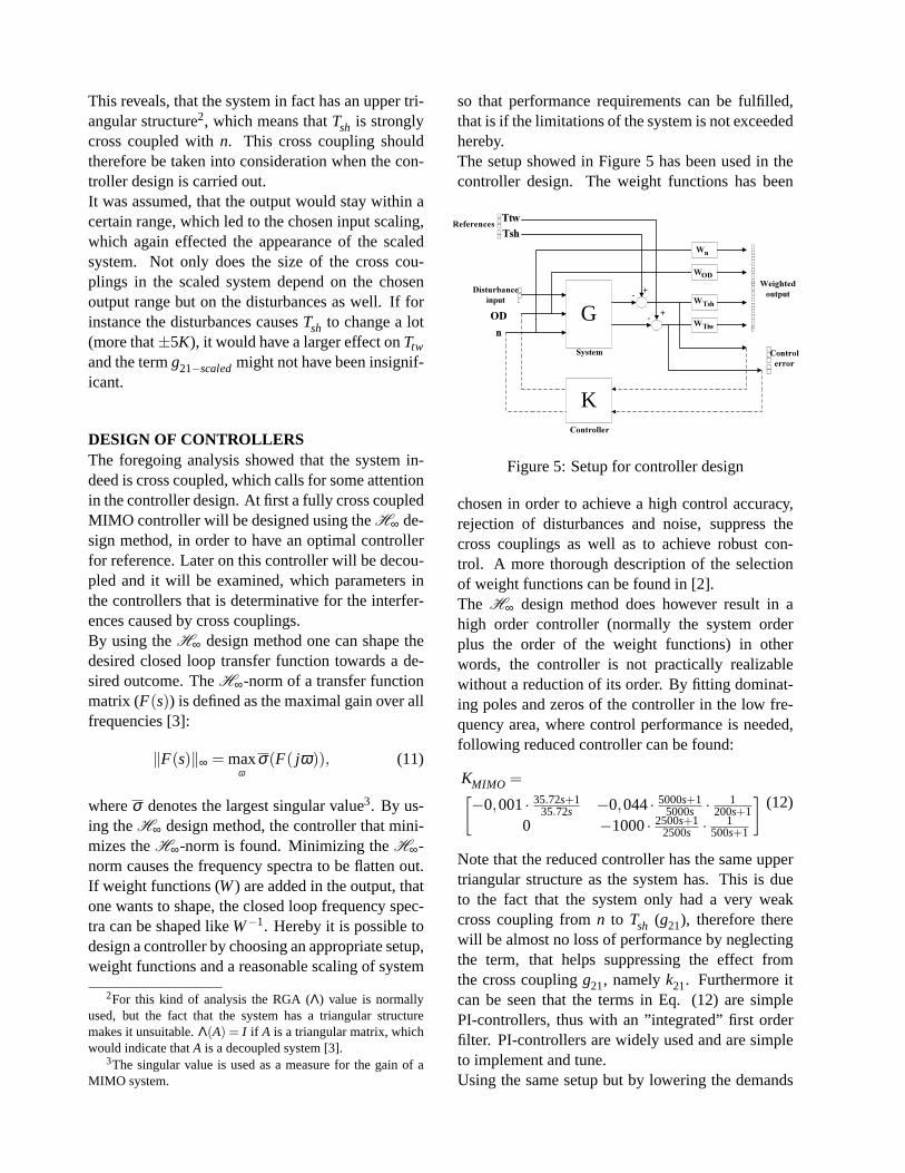
This reveals, that the system in fact has an upper tri-angular structure2, which means thatTsh is stronglycross coupled withn. This cross coupling shouldtherefore be taken into consideration when the con-troller design is carried out.It was assumed, that the output would stay within acertain range, which led to the chosen input scaling,which again effected the appearance of the scaledsystem. Not only does the size of the cross cou-plings in the scaled system depend on the chosenoutput range but on the disturbances as well. If forinstance the disturbances causesTsh to change a lot(more that±5K), it would have a larger effect onTtw

and the termg21−scaledmight not have been insignif-icant.

DESIGN OF CONTROLLERSThe foregoing analysis showed that the system in-deed is cross coupled, which calls for some attentionin the controller design. At first a fully cross coupledMIMO controller will be designed using theH∞ de-sign method, in order to have an optimal controllerfor reference. Later on this controller will be decou-pled and it will be examined, which parameters inthe controllers that is determinative for the interfer-ences caused by cross couplings.By using theH∞ design method one can shape thedesired closed loop transfer function towards a de-sired outcome. TheH∞-norm of a transfer functionmatrix (F(s)) is defined as the maximal gain over allfrequencies [3]:

‖F(s)‖∞ = maxω

σ(F( jω)), (11)

whereσ denotes the largest singular value3. By us-ing theH∞ design method, the controller that mini-mizes theH∞-norm is found. Minimizing theH∞-norm causes the frequency spectra to be flatten out.If weight functions (W) are added in the output, thatone wants to shape, the closed loop frequency spec-tra can be shaped likeW−1. Hereby it is possible todesign a controller by choosing an appropriate setup,weight functions and a reasonable scaling of system

2For this kind of analysis the RGA (Λ) value is normallyused, but the fact that the system has a triangular structuremakes it unsuitable.Λ(A) = I if A is a triangular matrix, whichwould indicate thatA is a decoupled system [3].

3The singular value is used as a measure for the gain of aMIMO system.

so that performance requirements can be fulfilled,that is if the limitations of the system is not exceededhereby.The setup showed in Figure 5 has been used in thecontroller design. The weight functions has been

G

K

5HIHUHQFHV

:7VK

:2'

:Q

:7WZ

7VK7WZ

'LVWXUEDQFHLQSXW2'Q

:HLJKWHGRXWSXW

&RQWUROHUURU

6\VWHP

&RQWUROOHU

+

+

-

-

Figure 5: Setup for controller design

chosen in order to achieve a high control accuracy,rejection of disturbances and noise, suppress thecross couplings as well as to achieve robust con-trol. A more thorough description of the selectionof weight functions can be found in [2].The H∞ design method does however result in ahigh order controller (normally the system orderplus the order of the weight functions) in otherwords, the controller is not practically realizablewithout a reduction of its order. By fitting dominat-ing poles and zeros of the controller in the low fre-quency area, where control performance is needed,following reduced controller can be found:

KMIMO =[−0,001· 35.72s+1

35.72s −0,044· 5000s+15000s · 1

200s+10 −1000· 2500s+1

2500s · 1500s+1

](12)

Note that the reduced controller has the same uppertriangular structure as the system has. This is dueto the fact that the system only had a very weakcross coupling fromn to Tsh (g21), therefore therewill be almost no loss of performance by neglectingthe term, that helps suppressing the effect fromthe cross couplingg21, namelyk21. Furthermore itcan be seen that the terms in Eq. (12) are simplePI-controllers, thus with an ”integrated” first orderfilter. PI-controllers are widely used and are simpleto implement and tune.Using the same setup but by lowering the demands

on the bandwidth of the controlled outputTtw, theother off diagonal term in the controller can beneglected and following controller achieved4:

KSISO=[−0,001· 35.72s+1

35.72s 00 −714· 2500s+1

2500s · 1500s+1

](13)

In Figure 6 is a step response from the linearized sys-tem showed, the response has been recorded at thestate around which the system was linearized givenby Eq.(6). As it can be seen is the response from the

Figure 6: Step response on the linearized systemmodel using a SISO and a MIMO controller

reference (Re f−Ttw) to Ttw a bit slower using theSISO controller in preference to the MIMO, whichof course is a result of the lowered demand on thebandwidth. Furthermore is the interference causedby the cross coupling (cross-interaction) larger us-ing the SISO controller, though the bandwidth ofthe controlled outputTtw in the MIMO controller ishigher. As it will be shown below, plays the requiredbandwidth ofTtw an important part in the magnitudeof the cross-interaction onTsh, when using a SISOcontroller.Using the fact that the system has an upper triangu-lar structure and two SISO controllers’ controls it,the open loop transfer function matrix can be writ-

4A high bandwidth is desirable as it gives a fast responseand a better rejection of disturbances

ten as:

GK =[g11 g120 g22

]·[k11 00 k22

]

=[g11k11 g12k22

0 g22k22

] (14)

The term in the off diagonalg12k22 is responsible forthe cross-interaction onTsh, like seen on the step re-sponse in the upper right plot in Figure 6. If thoughthe Tsh-controller is faster than this ”disturbance”(cross-interaction), then it will be able to suppress it.Illustrated in a Bode plot, see Figure 7, this meansthatg11k11 should cross the 0 dB gain (the cross overfrequency) at a higher frequency thang12k22

5, that isfollowing rule of thumb can be used:

• If ωc(g11k11) > ωc(g12k22) then the cross inter-action onTsh can be suppressed by the meansof a SISO control6.

ωc denotes the cross over frequency, see Figure 7.Hereby it can be seen that when one wants to sup-

Figure 7: A sketched open loop Bode plot for asystem were acceptable control can be achieved bySISO control

press the cross-interaction in the design of SISOcontrol, the task is to makek11 large andk22 low,that is the bandwidth of the superheat controller(k11) should be maximized whereas the bandwidthof water temperature controller (k22) should be min-imized. The bandwidth ofk22 should thus still besufficiently high to fulfill the required control per-formance.

5At low frequencies (below the cross over frequency) con-trol performance is needed, that is rejection of disturbances andkeeping track reference changes. Beyond the cross over fre-quency the task is to reject noise, that is to low pass filter

6This only holds ifg11k11 andg12k22 have nice behaviorswithout any resonance peaks as shown in Figure 7

Feedforward

A widely used technique to suppress the cross inter-action is feedforward. By making a feedforward ofthe control signal from compressorn to the valvecontrol OD, as shown in Figure 8, can the crossinteraction onTsh be suppressed to a great extent.Using the same notation as on Figure 8 the full con-

Figure 8: Feedforward of control signal from com-pressor.

trol can be written as:[OD1n1

]=

[k11 00 k22

]·[

eTsheTtw

]

+[0 f0 0

]·[ODn

] (15)

Sincen1 = n andn= k22eTtw Eq. 15 can be rewrittento:

[OD1n1

]=

[k11 f ·k220 k22

]·[

eTsheTtw

](16)

Hereby it can be seen that this way of using feedfor-ward, just is a special case of a MIMO controller.

RESULTSThe two designed controllersKMIMO (12) andKSISO(13) has been implemented on the test rig. They haveboth proven to be able to control as well the super-heatTsh as the water temperatureTtw. The main fo-cus has though been on the cross-couplings and sup-pressing the effects from these in the control. Bothof the controllers has been tested by making a largestep in the reference onTtw such that the control sig-nal n changes rapidly in order to initiate a visiblecross interaction onTsh. On Figure 9 is the responseon Tsh using these two controller shown. Note thatthe control signal to the compressorn saturates at4800 RPM, why the test data cannot directly be com-pared to the simulation, e.g. the step response onFigure 6. As it can be seen reduces the MIMO con-

Figure 9: Cross-interaction onTsh with SISO vs.MIMO control

troller the cross-interaction onTsh compared to theSISO controller, though the same changes has beenmade onn. This reduction is however only visiblewhen a very large bandwidth from theTtw-controller(k22) is required. This is in accordance to the rule ofthumb stated in the controller design; the largerk22compared tok11 the larger cross interaction.Using eitherKSISO or KMIMO to control the systemcan in practise only be seen on the size of the in-teraction coursed by the cross-coupling. It can beseen from eq. 13 and eq. 12 that the diagonal ele-ments almost are identical, why the step responsesalso are very alike except of course from the mag-nitude of the cross-interaction. This also appearsfrom the simulations showed on Figure 6, for thisreason only the response showing the effects fromthe cross-coupling has been included here.

CONCLUSIONSA dynamic lumped parameter model of a shell andtube condenser is presented. The model takes themass flow of refrigerant between gas- and liquid-phase into account whereby the subcooling can bedescribed. The full model consisting of the con-denser model, a dynamic moving boundary modelof the evaporator and static models of the compres-sor and valve posed good dynamic behavior as wellas static behavior.The structural analysis revealed that the system hasan upper triangular structure, that is, there is a crosscoupling from the rotational speed of the compressor

to the superheat. The importance of this cross cou-pling though depend on the asked for output rangeof the superheat and the water temperature and fur-thermore on the magnitude of the disturbances.By making a MIMO controller higher bandwidthof the water temperature control could be achieved,while keeping the cross interaction on the superheatto a minimum (in comparison to SISO control).For design of SISO controllers a rule of thumb wasstated, that gives a guideline to the design procedure,when the cross interaction is to be kept at a mini-mum.

REFERENCES

[1] John G. Collier. Convective Boiling and Con-densation. McGraw-Hill, 1 edition, 1972.

[2] L. Larsen and J. Holm. Modelling and control ofa refrigeration system. Master project at Tech-nical University of Denmark, 2002.

[3] S. Skogestad and I. Postlethwaite.Multivariablefeedback control, Analysis and Design. JohnWiley & Sons, 6 edition, 2001.

[4] G. L. Wedekind, B. L. Bhatt, and B. T. Beck.A system mean void fraction model for predict-ing various transient phenomena associated withtwo-phase evaporating and condensing flows.Int. J. Multiphase flow, 4:97–114, 1978.

[5] H. Xiang-Dong, Sheng Liu, and H. H. Asada.Modelling of vapor compression cycles for mul-tivariable feedback control of hvac systems.Journal of Dynamic Systems, Measurement andControl, 119:183–183, 1997.

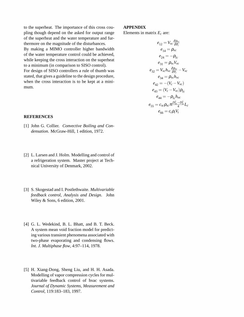
APPENDIXElements in matrixEc are:

e12 = Vvc∂ρvc∂Pc

e14 = ρvc

e24 =−ρlc

e31 = ρvcVvc

e32 = Vvchvc∂ρvc∂Pc

−Vvc

e34 = ρvchvc

e42 =−(Vc−Vvc)e43 = (Vc−Vvc)ρlc

e44 =−ρlchoc

e55 = cscρscπD2

oc−D2ic

4 Lc

e66 = ctρtVt