Aalborg Universitet

Comparison of Field Measurements and EMT Simulation Results on a Multi-LevelSTATCOM for Grid Integration of London Array Wind Farm

Glasdam, Jakob Bærholm; Kocewiak, Lukasz; Hjerrild, Jesper; Bak, Claus Leth; Zeni,LorenzoPublished in:Proceedings of the 45th 2014 CIGRE Session

Publication date:2014

Document VersionAccepted author manuscript, peer reviewed version

Link to publication from Aalborg University

Citation for published version (APA):Glasdam, J. B., Kocewiak, L., Hjerrild, J., Bak, C. L., & Zeni, L. (2014). Comparison of Field Measurements andEMT Simulation Results on a Multi-Level STATCOM for Grid Integration of London Array Wind Farm. InProceedings of the 45th 2014 CIGRE Session CIGRE (International Council on Large Electric Systems).

General rightsCopyright and moral rights for the publications made accessible in the public portal are retained by the authors and/or other copyright ownersand it is a condition of accessing publications that users recognise and abide by the legal requirements associated with these rights.

? Users may download and print one copy of any publication from the public portal for the purpose of private study or research. ? You may not further distribute the material or use it for any profit-making activity or commercial gain ? You may freely distribute the URL identifying the publication in the public portal ?

Take down policyIf you believe that this document breaches copyright please contact us at vbn@aub.aau.dk providing details, and we will remove access tothe work immediately and investigate your claim.

JAKGL@dongenergy.dk

Comparison of Field Measurements and EMT Simulation Results on a Multi-Level STATCOM for Grid Integration of London Array Wind Power Plant

Jakob Glasdam1,2, Łukasz Hubert Kocewiak1,

Jesper Hjerrild1, Claus Leth Bak2, Lorenzo Zeni1,3 1) DONG Energy Wind Power, 2) Aalborg University, 3) Technical University of Denmark

Denmark SUMMARY Simulation results are widely used in the design of electrical systems such as offshore wind power plants (OWPPs) and for determination of grid compliance. Measurements constitute an important part in the evaluation process of the OWPP, including passive and active components such as the static compensator (STATCOM). Quality measurement data allow the system designer to obtain real-life knowledge on the operating characteristics of the electrical component(s) for various operating scenarios of both the OWPP and the external grid. Furthermore, measurement data constitute an indispensable part of the evaluation of the simulation models of the OWPP components. The purpose of this paper is to develop and validate an electromagnetic transient (EMT) generic model of the modular multi-level cascaded converter (MMCC) STATCOM based on comparison with field measurements. For this purpose, measurement data have been acquired on a commercial ±50 MVAr state-of-the-art (SOA) MMCC STATCOM. The STATCOM is located at the point of common connection (PCC) at the world’s largest OWPP, London Array (LAOWPP). According to the authors’ knowledge, the presented paper will be the first of its kind to compare a detailed model of the STATCOM with actual field measurements for a commercial MMCC STATCOM. Furthermore, the paper offers the reader, being a researcher, transmission system operator, converter designer or a WPP developer etc., the unique opportunity to gain in-depth knowledge of the operating characteristics of the STATCOM for wind power integration, as well as of the validity of applying a generic model of the STATCOM without knowledge of the actual implemented control system. The proposed model is integrated into an aggregated EMT model of LAOWPP, which will be used to investigate possible resonance phenomena that will be shown in the paper to affect the harmonic distortion level. The STATCOM distortion level will be shown to be highly affected by the number of wind turbine generators (WTGs) in service. It will be shown that the inclusion of band rejection filters (BRFs) in the WTGs’ control loop lowers the STATCOM distortion level. It is found that the total inter-harmonic distortion (TIHD) index calculated according to IEC Standard 61000-4-7 is useful for assessing possible and undesired control interaction between the power electronic devices (PEDs) in OWPPs. The total harmonic distortion (THD) index, on the other hand, is found to contain very little information on possible PED controller interaction.

KEYWORDS Electromagnetic transient (EMT), field measurements, harmonic stability, model evaluation, modular multi-level cascaded converter (MMCC), offshore wind power plant (OWPP), static compensator (STATCOM), total inter-harmonic distortion (TIHD) index, voltage-source converter (VSC).

21, rue d’Artois, F-75008 PARIS B4_206_2014 CIGRE 2014 http : //www.cigre.org

2

1 Introduction Nowadays, offshore wind power penetration into the electrical grid is rapidly increasing and the current trend is to locate the OWPPs further from shore [1]. Flexible AC transmission system (FACTS) devices such as the STATCOM are commonly installed at the PCC in order to meet the reactive power requirements [2]. Modelling and simulation analysis has become an accepted and integral method in the design of electrical systems such as the OWPP [3]. The modelling approach must look for a right compromise between accuracy and computational speed. Furthermore, details regarding the internal behaviour of MMCC PEDs are often unknown or only partially known to the transmission system operator (TSO) and the OWPP developer. It is therefore crucial for these parties to assess the required modelling details and to gain confidence on the accuracy of the applied model. Therefore, field measurements have been collected on an MMCC STATCOM, which will be used in this paper to assess the MMCC STATCOM modelling requirements. Previous research on the modelling of the MMCC STATCOM has mainly been focused on the control system design and performance of the converter using a switching model (e.g. [4]), an analytical model (e.g. [5]) or a detailed model of the PED (e.g. [6]). None of these publications consider the accuracy of the model representation based on comparison with measurement data. The intention of this paper is to fill the gap, by providing a comparison between a generic, yet detailed STATCOM model and field measurements. Using the validated STATCOM model, the harmonic distortion level in the OWPP will be addressed in the time domain. Section 1.1 briefly outlines the peculiarities of possible control interaction between PEDs in an OWPP and possible methods to assess the controller interaction.

1.1 Harmonic Distortion in OWPPs OWPPs are susceptible to so-called “harmonic instability”, where the extensive sub-marine cabling and possible low available short-circuit power (ASCP) at the PCC may create resonance(s) within the bandwidth of the WTG controller bandwidth [7], [8], [9]. The result is unacceptable high harmonic distortion, which may cause disconnection of the WTG, unless countermeasures are taken. Disconnection of the WTG(s) is of course unacceptable, and harmonic stability studies are now an integral part of OWPP design studies. Currently, the studies are mainly done in the frequency domain [7], [9], where the assessment can be made based on algebraic formulation of the system and conventional indices such as the Nyquist stability criterion (NSC) can be applied. In [7] it was shown that the harmonic impedance in the OWPP is highly affected by the number of WTGs in service (#WTGiS). According to the authors’ experience it is therefore necessary to perform in the range of thousands of cases to cover all possible operating points of the OWPP and the external grid. This is straightforward in the frequency domain, whereas it is more challenging in the time domain, since the observed results do not contain information on the relative stability of the system. Furthermore, time-consuming model initialisation is also needed in the time domain. On the other hand, there are limitations to frequency domain analysis, as linearisation is done on both the non-linear switching devices as well as the control system. Furthermore, saturation effects of e.g. transformers and the integrator part of the PED proportional-integral (PI) controller are neglected. It is therefore useful to assess the controller interaction in both domains, i.e. calculate the NSC indices for the e.g. 2000 required study cases and then perform sensitivity analysis on the most critical cases in the time domain (e.g. for 50 cases). The authors are currently working on developing a procedure for addressing the controller interaction in OWPPs, taking into account the above-mentioned limitations in both the time and frequency domains. This paper will present how the harmonic distortion is affected by the #WTGiS and demonstrate how the time domain approach can be utilised in the assessment.

1.2 Paper Outline The remainder of the paper is organised as follows: Section 2 briefly describes the LAOWPP and the OWPP representation in the simulation tool. The installed STATCOM and the measurement setup are also briefly described. Section 3 presents the proposed model of the STATCOM, which will be evaluated in section 4 based on comparison with measurement data. Section 5 presents simulation results, in which the #WTGiS is varied and how this affects the STATCOM’s performance. Section 6 outlines concluding remarks. Section 7 outlines future work.

3

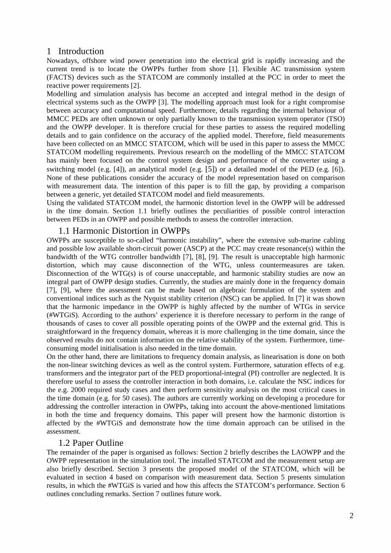
2 System Description The LAOWPP is located 20 km off the east coast of the UK at the mouth of the Thames, see Figure 1a. The OWPP is built in two phases, where Phase I was partly commissioned at the end of 2012. LAOWPP Phase I comprises 175 × 3.6 MW full-scale converter (FSC) WTGs, yielding a total capacity of 630 MW, making it the largest OWPP in the world. LAOWPP I is made up of four sections, and a simplified single-line diagram of one of these sections is shown in Figure 1b. As indicated in the figure, a combination of a STATCOM and a mechanically switched reactor (MSR) is connected to the tertiary winding of a 400/150/13.9 kV – 180/90/90 MVA onshore transformer in each of the four OWPP sections. The STATCOM is equipped with 22 full-bridge sub-modules (SMs) per phase, where two are redundant, but still in service during normal operating mode [10]. The efficient operating number of SMs is therefore 𝑁 = 20, resulting in a 41-level line voltage waveform. Figure 1b also indicates the locations of the installed voltage and current transducers (VTs and CTs, respectively). Flexible Rogowski coil CTs with a minimum bandwidth of 55 mHz – 3 MHz [11] were used together with custom made capacitive voltage dividers with bandwidth of 1 Hz – 1 MHz [12]. The sampling rate was set at 51.2 kS/s/ch for approximately half the duration of the measurement campaign and at 102.4 kS/s/ch for the remainder of the one-month measurement campaign, resulting in approximately 11 TB of data (12 channels). Figure 1c shows a more detailed three-phase diagram of the STATCOM. The locations of the installed transducers as well as the symbols of the electrical quantities used in the paper are shown.

London

D ungrounded

33/150 kV 400 kV

13.9 kV

MSR

MMCC STATCOM

PCC

=temporary installed

transducers

C-filter

Filter

Shore

Wye connected

=Existing power quality measurement

equipment

C2RLC1

CBA

Phase

A

Phase C

Phase B

Measurement points

ci,2bai

,1bai

,1cbi

,2cbi

,1aci

,2aci1au

1bu

1cu

2au

2bu2cu

,a cu

,b cu

,c cu

1 1ab a bu u u= −bcu cau

Voltage: Current:

,1 ,2a ba aci i i= − bi

a) Geographical location of the LAOWPP.

b) Simplified single line diagram of one of the four sections of the

LAOWPP.

c) Simplified three-phase diagram of the STATCOM and associated filter.

Figure 1 Location and single line diagram of the LAOWPP and three-phase diagram of the STATCOM.

2.1 London Array OWPP Representation A simplified representation of the LAOWPP has been implemented in an EMT platform, as will be briefly described. Only one of the four sections is modelled. The WTGs located in the section are aggregated into one equivalent two-level FSC WTG. This is considered appropriate, as explicit representation of the individual WTGs significantly increases the modelling order and compromises the simulation speed dramatically. Furthermore, the main focus in this paper is on the performance of the proposed STATCOM model. The authors intend to evaluate this simplification in future work. The generator side of the converter is represented by a first-order DC Norton equivalent with a time constant of 𝑇 =100 ms, adapted from [13], see Figure 2b. Figure 2a shows the inner current control system, operating in the rotating reference frame (RRF). Band rejection filters (BRFs) have been included in the control loop according to the recommendation in [9] to improve the relative harmonic stability of the system. The transfer function of the BRF is given in canonical form in (1) [7], where the damping coefficient is selected as 𝜁 = 1 √2⁄ . 𝑠 is the Laplace operator. 𝜔𝑛,𝐵𝑅𝐹 is the tuned angular frequency in [rad/s], which has been selected as

4

𝜔𝑛,𝐵𝑅𝐹 = 2𝜋 × 118 Hz based on Fourier transformation on the simulation results. Tuning of the BRF is normally done using frequency domain analysis [7], [9], for reasons described in section 1.1. As will be shown in section 5, the BRF tuned at this frequency significantly improves the harmonic content in the STATCOM’s output currents and voltages over the full range of #WTGiS of the LAOWPP.

𝐺𝐵𝑅𝐹(𝑠) =�𝑠 𝜔𝑛,𝐵𝑅𝐹⁄ �

2 + 1

�𝑠 𝜔𝑛,𝐵𝑅𝐹⁄ �2 + 2𝜁�𝑠 𝜔𝑛,𝐵𝑅𝐹⁄ � + 1

(1)

The 33 kV cable collection grid is aggregated into one nominal PI section with a length of 1 km, which is considered sufficient for the frequency range considered in the current work. The approximately 50-km-long 150 kV export cable is modelled using the “Frequency-Dependent Phase Model” in the EMT simulation tool. No information of actual ASCP has been available, hence the 400 kV grid is represented by a 22 GVA Thevenin equivalent with 𝑋 𝑅⁄ = 22, given in the as-built documentation of the LAOWPP.

,d qu,PCC ju

,c ji

*ju

PLLθ*

,d qu

( , , )j a b c=

abc

abcabcCurrent

controller

*,dqi

,d qi

BRF

BRF

RRF

RRF

RRF

PLLθ

chopRdci

dcu11sT +

dcu

dcPmechP

*ju

,c ji ,PCC judci

Filterbank

a) Inner-loop current controller. b) Simplified WTG model.

Figure 2 Aggregated model of the WTG and inner-loop controller in the RRF. Command signals 𝑖𝑑∗ and 𝑖𝑞∗ in a) are provided by two outer-loop controllers responsible for controlling 𝑢𝑑𝑐 and 𝑈𝑃𝐶𝐶,𝑅𝑀𝑆 , respectively.

3 STATCOM MMCC Modelling The MMCC STATCOM consists of a number of distributed DC voltages, which are incrementally inserted or bypassed in order to synthesise a high-quality sinusoidal voltage waveform. The MMCC technology was extended to the voltage source converter high-voltage direct current (VSC-HVDC) system in [14] and is now considered SOA [1]. A detailed representation of the MMCC STATCOM has been implemented in an EMT simulation tool, where all the internal dynamics usually relevant for EMT studies (i.e. generated harmonics due to switching of the converter, individual SM capacitor charging etc. [15]) are taken into account. Losses due to the commutation process are not included, as only the SM terminal and capacitor conditions are of relevance in this work, which is in accordance with the guidelines given in [16] for power system studies. The relatively high number of switching elements in the MMCC STATCOM possesses some challenges in EMT simulation tools, as a high computational effort is required for re-triangularisation of the electrical network subsystem admittance. Based on the “Nested Fast and Simultaneous Solution” [17], an efficient and accurate representation of each of the phase legs of the MMCC VSC-HVDC was proposed in [15]. A similar modelling approach has been taken in this work for the STATCOM phase leg, as will be described with reference to Figure 3.

1SMn =

,1dcu

,2dcu

,dc Nun N=

2n =

legu

Main EMT electrical

solver

ini

Norton Eq.

legu ,

,

EQ leg

EQ leg

uR,

1

EQ legR

a) Series connection of N=20 full-bridge SMs in the STATCOM

phase leg.

b) Electrical equivalent of figure a.

c) Aggregated Norton equivalent of the STATCOM phase leg and

interface with the main EMT solver. Figure 3 Derivation of Norton equivalent representation of the STATCOM phase leg.

Firstly, the large number of IGBT/diode pairs and distributed capacitances in the phase leg in Figure 3a are represented by their electrical equivalent, as in Figure 3b. The SM capacitance can be represented by its Norton equivalent by applying the trapezoidal integration rule according to

5

Dommel’s formulation [15]. By calculation of the input impedance of the nth (𝑛 = 1,2, …𝑁 = 20) SM and calculating the SM capacitor voltage (𝑢𝑑𝑐,𝑛) in each SM, it is possible to aggregate the N SMs into a single Norton equivalent as shown in Figure 3c, where 𝑢𝐸𝑄,𝑙𝑒𝑔 is given in (2):

𝑢𝐸𝑄,𝑙𝑒𝑔 = �𝑢𝑑𝑐,𝑛

𝑁

𝑛=1

(2)

Similarly, 𝑅𝐸𝑄,𝑙𝑒𝑔 is the summation of the calculated input impedances of the 𝑁 SMs in Figure 3b. By using the Norton equivalent in Figure 3c, the number of frequently switched branches in the resulting network admittance matrix is thereby significantly reduced, while all branch current and node voltage information is retained within the Norton equivalent and accessible to the main EMT solver. The authors are currently preparing the description of the derivation of the Norton equivalent, which will be presented in future work.

3.1 STATCOM Control System One of the main challenges related to MMCCs is the control of the distributed SM capacitor voltages dynamically as well as in steady-state [1]. A brief description of the implemented controller will be given in the following, with reference to Figure 4. Figure 4a shows the upper-level controller, which is a conventional cascaded PI controller with the inner-loop current controller operating in the RRF. The two outer loops are responsible for controlling the PCC reactive power (𝑄𝑃𝐶𝐶) (𝑞-axis) and the average SM capacitor voltage of the three phases (𝑢𝑑𝑐,𝐴𝑉) in the 𝑑-axis, respectively. 𝑢𝑑𝑐,𝐴𝑉 is calculated as in (3) and is compared with rated SM voltage (𝑢𝑑𝑐,𝑠𝑀

∗ ) in the outer control loop.

𝑢𝑑𝑐,𝐴𝑉 =1

3𝑁��𝑢𝑑𝑐,𝑗,𝑛

𝑁

𝑛=1

𝐽=3

𝑗=1

(3)

The converter phase leg voltage controller in Figure 4b controls the average converter leg voltage (𝑢𝑑𝑐,𝐴𝑉,𝑗 = 1 𝑁⁄ ∑ 𝑢𝑑𝑐,𝑗,𝑛

𝑁𝑛=1 ) in the 𝑗𝑡ℎ phase leg (𝑗 = 𝑎, 𝑏, 𝑐) to follow 𝑢𝑑𝑐,𝐴𝑉 from (3). The output

of the P4 controller in the 𝑗𝑡ℎ phase is then multiplied by a cosine wave which is in phase with 𝑢𝑐,𝑗∗

obtained from Figure 4a. Summing the output of the three P4 phase controllers is then a zero-sequence reference current 𝑖0∗. In the existence of an imbalance between the phase leg voltages, e.g. 𝑢𝑑𝑐,𝐴𝑉 >𝑢𝑑𝑐,𝐴𝑉,𝑎, the product of 𝑢𝑎,𝑐 ∙ 𝑖0 forms a positive active power charging the capacitors in phase leg A in Figure 1c. The current loop forces 𝑖0 to follow its command signal 𝑖0∗.

SRF

PLLθ

+- PI2 *di

di

+

-

+

-

PI1

+ -*qi

qiLpu

Lpu

PI3

PI3

abcSRF

*du

du

*qu

qu

+

*,dc SMu

,PCC juPLLθ

,dc AVu

*,c ju,c ji

( , , )j a b c=

+++ +

abc

RRF

abc

RRF

RRF

*uβ

*uα

*PCCQ

PCCQ

= stationarySRFreference frame

a) Upper-level controller with current controller operating in

the RRF.

,dc AVu +

- P6

, ,dc j nu *, ,dc j nu

,2ki( , , )k ba cb ac=

c-i) Individual SM controller.

*0u

*,j nu

++

++

*,c ju

Common reference signal

for all SMs in the jth phase

Individual reference signal for the nth SM in

the jth phase

*, ,dc j nu

c-ii) Reference signal for the 𝑛𝑡ℎ SM.

Valve DC voltage controller

Zero sequence current controller

Σ

+

- P4

, ,dc AV cu ( )*cos 2 3θ π+

, ,dc AV bu

+

- P4

( )*cos 2 3θ π−

+

-

, ,dc AV auP4

( )*cos θ

Σ*0i

1 3

+

-

0iP5

,dc AVu

( )* 1 * *tan u uβ αθ −=

,1aci,1bai,1cbi

*',c ju

4,nS 3,nS

2,nS1,nS

1−

1

0

[ ]p.u

Time

( )y t2π2π−

[ ]s

π0π−

*,j nuCarrier for and 3,nS

4,nS

1,nS

2,nS

b) Phase-valve voltage and zero-sequence current controller. d) POD PSCPWM for the 𝑛𝑡ℎ SM.

Figure 4 Implemented STATCOM controller. Figure c) – i) shows the individual capacitor voltage controller for the 𝑛𝑡ℎ SM in 𝑗𝑡ℎ phase (𝑗 = 𝑎, 𝑏, 𝑐). Figure c) – ii) shows the reference signal for the 𝑛𝑡ℎ SM.

6

A distributed SM voltage controller has been included as shown in Figure 4c-𝑖. The controller is responsible for maintaining the capacitor voltage of the 𝑛𝑡ℎ SM in the 𝑗𝑡ℎ phase (𝑢𝑑𝑐,𝑗,𝑛) at the reference value 𝑢𝑑𝑐,𝐴𝑉. The controller forms an active power between 𝑢𝑑𝑐,𝑗,𝑛 and the leg current (𝑖𝑘,2 (𝑘 = 𝑏𝑎, 𝑐𝑏,𝑎𝑐), see Figure 1c) [18]. In [19] it was shown that no coupling exists between the zero-sequence current controller in Figure 4b and the individual SM controller in Figure 4c-𝑖. Figure 4c-𝑖 shows the addition of the reference signals from the three main controllers in Figure 4a, b and c. The resulting reference signal 𝑢𝑗,𝑛

∗ for the 𝑛𝑡ℎ SM (𝑛 = 1,2, …𝑁) in the 𝑗𝑡ℎ phase (𝑗 = 𝑎, 𝑏, 𝑐) is then fed to a modulator, where it is compared to a triangular-wave carrier (𝑇𝑊𝐶𝑛, 𝑛 = 1,2, …𝑁) that is individual for the 𝑛𝑡ℎ SM (Figure 4d). Phase opposition disposition (POD) phase-shifted carrier-based pulse-width modulation (PSCPWM) [20] with a phase shift of 𝜃𝑝𝑠 = 2𝜋(𝑛 − 1)/𝑁 between two adjacent carriers (e.g. 𝑇𝑊𝐶𝑛 and 𝑇𝑊𝐶𝑛+1) has been used. The frequency of the carriers has been selected as 𝑓𝑇𝑊𝐶𝑛 = 3.37∙50 Hz. This value of 𝑓𝑇𝑊𝐶𝑛 has been chosen as a non-integer pulse number has a balancing effect on the SM capacitors [21]. It should be noted that no information on the applied modulation technique of the actual STATCOM is publicly available and was thus not available to the authors. Based on the comparison between measurement and simulation results in section 4 (Figure 6b), it is evident that the model with the described modulation technique is highly capable of replicating the switching actions of the actual STATCOM. The applied modulation technique in the model is therefore considered viable. The modulation technique will be more carefully investigated based on post-processing of the collected one-month measurement data in future work.

4 Model Evaluation The proposed model of the MMCC STATCOM described in section 3 will be validated based on comparison with obtained measurement results during steady-state operating mode and during a transition from 𝑄 = −0.73 p.u to 𝑄 = −0.79 p.u. The evaluation will be based on a qualitative approach comparing measurement and simulation results and will be done in the time domain. Figure 5 shows the measured converter terminal voltages and the line currents during steady state (see Figure 1c). Subscripts “m” and “s” denote measurement and simulation, respectively. As evident from the figure, the measurement system is capable of capturing the measured waveforms with high resolution. The figure also clearly shows that the converter terminal voltages with a good approximation appear to be sinusoidal waveforms due to the MMCC technology. Very little harmonic residue is present in the output line current as also replicated in the simulation.

a) Measured and simulated leg voltages. b) Measured and simulated line currents.

Figure 5 Comparison between measurement and simulation during steady-state operating mode. Subscripts “m” and “s” denote measurement and simulation, respectively.

Figure 6a shows the phase A converter leg and phase A to B line voltages (𝑢𝑎,𝑐 and 𝑢𝑎𝑏, respectively, see Figure 1c) during a shorter time span, in order to more clearly show the high quality of the measurements and the validity of the proposed model. The incremental step increase in the converter voltage is clearly observable in the measurement and well replicated by the simulation results (𝑢𝑎,𝑐,𝑚 and 𝑢𝑎,𝑐,𝑠, respectively). The model is to a high extent capable of replicating the measured variation in 𝑢𝑎,𝑐,𝑚 caused by the switching action of the STATCOM. It should be noted that an imbalance in the line voltages was sustained throughout the measurement period as shown in Figure 6b. The voltage imbalance has been compensated for by adjusting the amplitude of the individual Thevenin phase voltage sources. This is considered appropriate since no detailed information of the external grid was available.

0 5 10 15 20 25 30 35 40-1

-0.8-0.6-0.4-0.2

00.20.40.60.8

1

Time [ms]

Volta

ge [p

.u]

u

a,c,m u

a,c,s u

b,c,m u

b,c,s u

c,c,m u

c,c,s

0 5 10 15 20 25 30 35 40-1

-0.8-0.6-0.4-0.2

00.20.40.60.8

1

Time [ms]

Curr

ent [

p.u]

i

a,m i

a,s i

b,m i

b,s i

c,m i

c,s

7

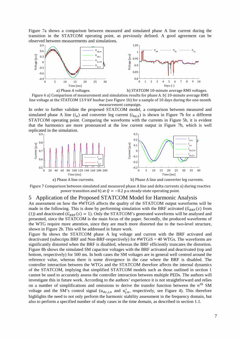
Figure 7a shows a comparison between measured and simulated phase A line current during the transition in the STATCOM operating point, as previously defined. A good agreement can be observed between measurements and simulations.

a) Phase A voltages. b) STATCOM 10-minute average RMS voltages.

Figure 6 a) Comparison of measurement and simulation results for phase A. b) 10-minute average RMS line voltage at the STATCOM 13.9 kV busbar (see Figure 1b) for a sample of 10 days during the one-month

measurement campaign. In order to further validate the proposed STATCOM model, a comparison between measured and simulated phase A line (𝑖𝑎) and converter leg current (𝑖𝑏𝑎,2) is shown in Figure 7b for a different STATCOM operating point. Comparing the waveforms with the currents in Figure 5b, it is evident that the harmonics are more pronounced at the low current output in Figure 7b, which is well replicated in the simulation.

a) Phase A line currents. b) Phase A line and converter leg currents.

Figure 7 Comparison between simulated and measured phase A line and delta currents a) during reactive power transition and b) at 𝑄 = −0.2 p.u steady-state operating point.

5 Application of the Proposed STATCOM Model for Harmonic Analysis An assessment on how the #WTGiS affects the quality of the STATCOM output waveforms will be made in the following. This is done by performing simulation with the BRF activated (𝐺𝐵𝑅𝐹(𝑠) from (1)) and deactivated (𝐺𝐵𝑅𝐹(𝑠) = 1). Only the STATCOM’s generated waveforms will be analysed and presented, since the STATCOM is the main focus of the paper. Secondly, the produced waveforms of the WTG require more attention, since they are much more distorted due to the two-level structure, shown in Figure 2b. This will be addressed in future work. Figure 8a shows the STATCOM phase A leg voltage and current with the BRF activated and deactivated (subscripts BRF and Non-BRF-respectively) for #WTGiS = 40 WTGs. The waveforms are significantly distorted when the BRF is disabled, whereas the BRF efficiently truncates the distortion. Figure 8b shows the simulated SM capacitor voltages with the BRF activated and deactivated (top and bottom, respectively) for 500 ms. In both cases the SM voltages are in general well centred around the reference value, whereas there is some divergence in the case where the BRF is disabled. The controller interaction between the WTGs and the STATCOM therefore affects the internal dynamics of the STATCOM, implying that simplified STATCOM models such as those outlined in section 1 cannot be used to accurately assess the controller interaction between multiple PEDs. The authors will investigate this in future work. According to the authors’ experience it is not straightforward and relies on a number of simplifications and omissions to derive the transfer function between the 𝑛𝑡ℎ SM voltage and the SM’s control signal (𝑢𝑑𝑐,𝑗,𝑛 and 𝑢𝑗,𝑛

∗ , respectively, see Figure 4). This therefore highlights the need to not only perform the harmonic stability assessment in the frequency domain, but also to perform a specified number of study cases in the time domain, as described in section 1.1.

0 5 10 15 20 25 30-0.9

-0.6

-0.3

0

0.3

0.6

0.9

Time [ms]

Volta

ge [p

.u]

u

ab,m u

ab,s u

a,c,m u

a,c,s

0 1 2 3 4 5 6 7 8 9 100.8

0.85

0.9

0.95

1

1.05

Days [-]

Volta

ge [p

.u]

uab ubc uca

0 20 40 60 80 100 120 140 160 180 2000.5

0.6

0.7

0.8

0.9

Time [ms]

Curr

ent [

p.u]

ia,m

ia,s

0 5 10 15 20 25 30 35 40-0.3

-0.2

-0.1

0

0.1

0.2

0.3

Time [ms]

Curr

ent [

p.u]

i

a,m i

a,s i

ba,2,m i

ba,2,s

8

Calculating the total harmonic (THD) indexes over 10 cycles on the converter leg voltages in Figure 8a using the method described in the following results in THDBRF = 0.083 p.u and THDNon-BRF = 0.077 p.u for the two cases. This is very misleading, as observed from the figure. Calculating the total inter-harmonic distortion (TIHD) indexes yields TIHDBRF = 0.065 p.u and TIHDNon-BRF = 0.124 p.u, which is in better correlation with Figure 8a. The THD index alone does therefore not indicate possible harmonic controller interaction. The TIHD index will therefore be introduced in the stability assessment.

a) Phase A leg voltage and current with the BRF activated and deactivated for #WTGiS = 40 WTGs.

b) SM voltages for phase A leg with BRF enabled

and disabled (top and bottom, respectively). c) Calculated THD (top) and TIHD with BRF enabled

and disabled (red and blue, respectively). Figure 8 Simulation results for the STATCOM and c) calculated THD and TIHD as a function of #WTGiS.

The THD and TIHD are calculated according to IEC 61000-4-7 [22], where the sampling interval (SI) is fixed at 10 cycles for fundamental frequency (𝑓1 = 50 Hz). Thus frequency bins in the discrete spectrum estimated using discrete Fourier transform are with Δ𝑓 = 5 Hz resolution. The standard proposes to group the spectra into harmonic and inter-harmonic subgroups (HSGs and IHGs, respectively). The HSG for the 𝑛𝑡ℎ harmonic (𝑛 = 2,3, …𝑁 = 50) consists of the 𝑛 ∙ 𝑓1 harmonic component and the two adjacent frequency bins (e.g. {95, 100, 105 Hz} from the HSG of second harmonic (𝑛 = 2)). Similarly, the seven frequency bins {60, 65,…, 90 Hz} from the first IHG (𝑛 = 1). The THD is defined as the ratio of the RMS value of the harmonic subgroups (HSGs) to the RMS value of the 𝑓1 component (𝑈1) as in (4-a), where 𝑈(𝑛 ∙ 𝑓1 + 𝑖 ∙ Δ𝑓) is the RMS value of the 𝑛 ∙ 𝑓1 + 𝑖 ∙Δ𝑓 frequency bin. The TIHD is calculated similarly, as in (4-b).

𝑇𝐻𝐷 =

�∑ ��∑ [𝑈(𝑛 ∙ 𝑓1 + 𝑖 ∙ 𝛥𝑓)]2𝐼=1 𝑖=−1 �

2𝑁𝑛=2

𝑈1=

�∑ �∑ [𝑈(𝑛 ∙ 𝑓1 + 𝑖 ∙ 𝛥𝑓)]2𝐼=1 𝑖=−1 �𝑁

𝑛=2

𝑈1

[p.u] (4-a)

𝑇𝐼𝐻𝐷 =�∑ �∑ [𝑈(𝑛 ∙ 𝑓1 + 𝑖 ∙ 𝛥𝑓)]2𝐼=8

𝑖=2 �𝑁𝑛=1

𝑈1 [p.u] (4-b)

In order to correlate the harmonic stability of the OWPP with #WTGiS, Figure 8c shows the calculated THDBRF and THDNon-BRF (top figure) and TIHDBRF and TIHDNon-BRF (bottom figure). A resolution of Δ#WTGiS =5 WTG/bin is used. Furthermore, the case with #WTGiS = 36 WTGs is also included, as this is where the controller interaction becomes critical, as can also be noted from the spike at TIHDNon-BRF(36) in the bottom figure in Figure 8c. There is a relatively good correlation between the THDBRF and THDNon-BRF for all considered cases up to #WTGiS = 55 WTGs, which again implies that the THD index alone is insufficient in the assessment. A similar correlation between TIHDBRF and TIHDNon-BRF is observed for #WTGiS ≤ 35

40 42 44 46 48 50 52 54 56 58 60 62 64 66 68 70 72 74 76 78 80-1.20-0.80-0.400.000.400.801.20

Time [ms]

Volta

ge &

curr

ent [

p.u]

u

a,c,BRF u

a,c,Non-BRF i

ba,BRF i

ba,Non-BRF

0 50 100 150 200 250 300 350 400 450 5000.95

1.00

1.05

Volta

ge [p

.u]

0 50 100 150 200 250 300 350 400 450 5000.95

1.00

1.05

Volta

ge [p

.u]

Time [ms]

5 10 15 20 25 30 35 40 45 50 550.00

0.04

0.08

0.12

THD

[p.u

]

BRF Non-BRF

5 10 15 20 25 30 35 40 45 50 550.040.080.120.16

TIHD

[p.u

]

# WTGs in service [-]

9

WTGs. The TIHDBRF is relatively constant for #WTGiS ≤ 45. The TIHDBRF approaches TIHDNon-BRF for #WTGiS > 45, indicating that the BRF is not capable to supress the controller interaction for this range of #WTGiS. The harmonic impedance of the OWPP (𝑍𝑂𝑊𝑃𝑃(𝜔, #WTGiS)) and the corresponding resonance frequency (𝜔𝑟(#WTGiS)) are functions of #WTGiS, as described in section 1.1. The high number of #WTGiS most likely causes 𝜔𝑟(≥ 50WTG) to be shifted away from 𝜔𝑛,𝐵𝑅𝐹, meaning that the BRF is not capable of affectively attenuating the resonance. Frequency domain techniques would be useful to assess the frequency-dependent characteristics and the change in resonances. The TIHDBRF could be improved by e.g. increasing the bandwidth of the BRF, which might deteriorate the NSC at other frequencies and is therefore not desired [7]. Another viable option would be to apply adaptive BRFs in the WTG controller [7]. The inclusion of BRFs in the STATCOM control system could also be considered. The studied system has in this work been one section of the LAOWPP, where the average number of installed WTGs per section is 175/4 ≃ 45. Based on Figure 8c, it can therefore be concluded that the OWPP section is stable for all possible #WTGiS, when using the BRF tuned at 118 Hz in the WTG and considering that generic models have been used to represent both the aggregated WTG and the STATCOM. Furthermore, the highest possible ASCP at the PCC has been used in this work. It is therefore also necessary to assess the harmonic distortion as a function of ASCP in order to assess the overall stability of the system. The possible effect of the remaining three OWPP sections should also be investigated. The purpose of this section has been to investigate the application of time domain analysis in the harmonic stability assessment and not the actual stability of the system, which will be considered more carefully in future work.

6 Conclusion The paper has presented a generic, yet detailed model of the MMCC STATCOM and compared the results with high-quality measurement data collected on an actual MMCC-based STATCOM for wind integration. It was found that the generic developed STATCOM model is capable of replicating the measured waveforms with good accuracy. A generic model of the STATCOM is therefore suitable in the preliminary design phase of an OWPP, before an agreement with a specific vendor is made. The paper has outlined the necessity to assess the harmonic stability in the design phase of an OWPP and pointed out advantages of time and frequency domain analysis methods. Using the proposed model of the STATCOM, the harmonic stability assessment has been addressed in the time domain, where the #WTGiS was varied to investigate the controller interaction between the WTGs and the STATCOM. It was found that the interaction becomes noticeable for #WTGiS ≥ 36 WTGs, unless countermeasures are taken. It was found that the total inter-harmonic distortion (TIHD) index according to IEC Standard 61000-4-7 is useful to assess possible and undesired control interaction between the PEDs in OWPPs. It was shown that an application of active filtering in the WTGs by means of BRF (i.e. notch filter) in the main control chain can potentially reduce harmonic emission at the point of interest (e.g. PCC) and improve overall stability in OWPPs. This can be achieved by reducing the harmonic content generated by the converters as well as changing existing resonances (i.e. improving damping or shifting resonance frequencies). Improving the converters controllers rejection capability called active damping is a certain type of active filtering. The converter may be controlled adaptively or tuned to suppress selected harmonic components. Thus there is no need to interfere with the OWPP design.

7 Future Work The authors intend in future work to more carefully correlate frequency and time domain analysis for harmonic stability studies and are currently developing a procedure for assessment of the harmonic stability in AC and VSC-HVDC-connected OWPPs. More robust mitigation methods than the BRF used here will be investigated for. An aggregated representation of the WTGs was used in the current work, since this has a significant impact on simulation speed. The appropriateness of this simplification for harmonic stability studies will be investigated in the time and frequency domains. The derivation of the detailed MMCC STATCOM model will be more carefully described, and the authors intend to investigate the applicability of more simplified generic RMS and EMT models of the MMCC STATCOM for harmonic stability studies. A statistical analysis of the one-month measurement data will be presented in future work, where the generated harmonics will be investigated based on e.g. power system frequency variation, OWPP power production level, STATCOM operating point etc.

10

BIBLIOGRAPY [1] J. Glasdam, J. Hjerrild, L. H. Kocewiak and C. L. Bak, "Review on multi-level voltage source

converter based HVDC technologies for grid connection of large offshore wind farms" (Power System Technology (POWERCON), 2012 IEEE International Conference on, 2012, pp. 1--6.)

[2] M. Pereira, D. Retzmann, J. Lottes, M. Wiesinger and G. Wong, "SVC PLUS: An MMC STATCOM for network and grid access applications," (PowerTech, 2011 IEEE Trondheim, 2011, pp. 1--5.)

[3] J. Glasdam, C. L. Bak and J. Hjerrild, "Transient studies in large offshore wind farms employing detailed circuit breaker representation," (Energies, vol. 5, no. 7, pp. 2214--2231, 2012.)

[4] S. Sirisukprasert, A. Q. Huang and J. S. Lai, "Modeling, analysis and control of cascaded-multilevel converter-based STATCOM," (PES General Meeting, 2003, IEEE, vol. 4, 2003.)

[5] J. Kumar, B. Das and P. Agarwal, "Modeling of 11-Level Cascade Multilevel STATCOM," (International Journal of Recent Trends in Engineering, vol. 2, no. 5, 2009.)

[6] T. S. Yeh, H. F. Jhu and H. W. Sung, "Modeling and control of three-phase multilevel inverter-based STATCOM," (Power Electronics for Distributed Generation Systems (PEDG), 2010 2nd IEEE International Symposium on, 2010, pp. 406--411.)

[7] L. Kocewiak, "Harmonics in large offshore wind farms," (PhD Thesis, Department of Energy Technology, Aalborg University, Aalborg, 2012.)

[8] Ł. H. Kocewiak, J. Hjerrild and C. Leth Bak, "Wind turbine converter control interaction with complex wind farm systems," (IET Renewable Power Generation, vol. 7, no. 4, Nov. 2013.)

[9] P. Brogan, "The Stability of Multiple, high power, active front end voltage sourced converters when connected to wind farm collector systems," (Proc. 2010 EPEC, 2010.)

[10] M. Pereira, M. Pieschel and R. Stoeber, "Prospects of the new SVC with Modular Multilevel Voltage Source Converter," (CIGRE Colloquium, October, 2011.)

[11] Powertek, “CWT and CWT LF wideband current probes for high frequency high current measurement,” (Accessed online Dec, 2013, http://www.powertekuk.com/cwt.htm)

[12] L. Christensen, et al., "GPS synchronized high voltage measuring system," (Nordic Wind Power Conference, nov., 2007.)

[13] S. K. Chaudhary, "Control and Protection of Wind Power Plants with VSC-HVDC Connection," (PhD Thesis, Aalborg University, Aalborg, Denmark, 2011.)

[14] A. Lesnicar and R. Marquardt, "An innovative modular multilevel converter topology suitable for a wide power range," (Power Tech Conference Proc., 2003 IEEE Bologna, vol. 3, 2003, pp. 6)

[15] U. N. Gnanarathna, A. M. Gole and R. P. Jayasinghe, "Efficient modeling of modular multilevel HVDC converters (MMC) on electromagnetic transient simulation programs," (Power Delivery, IEEE Transactions on, vol. 26, no. 1, pp. 316--324, 2011.)

[16] A. Gole, et al., "Guidelines for modeling power electronics in electric power engineering applications," (Power Delivery, IEEE Transactions on, vol. 12, no. 1, pp. 505--514, 1997.)

[17] K. Strunz and E. Carlson, "Nested fast and simultaneous solution for time-domain simulation of integrative power-electric and electronic systems," (Power Delivery, IEEE Transactions on, vol. 22, no. 1, pp. 277--287, 2007.)

[18] M. Hagiwara and H. Akagi, "Control and experiment of pulsewidth-modulated modular multilevel converters," (Power Electronics, IEEE Transactions on, vol. 24, no. 7, pp. 1737--1746, 2009.)

[19] M. Hagiwara, R. Maeda and H. Akagi, "Negative-Sequence Reactive-Power Control by a PWM STATCOM Based on a Modular Multilevel Cascade Converter (MMCC-SDBC)," (Industry Applications, IEEE Transactions on, vol. 48, no. 2, pp. 720--729, 2012.)

[20] D. G. Holmes and T. A. Lipo, “Pulse Width Modulation for Power Converters: Principles and Practice,” (IEEE Press, 2003.)

[21] G. Asplund, "Method for controlling a voltage source converter and a voltage converting apparatus," (US Patent 20,100,328,977, Dec. 30, 2010.)

[22] International Electrotechnical Commission, IEC 61000-4-7, “Testing and measurement techniques—General guide on harmonics and interharmonics measurements and instrumentation, for power supply systems and equipment connected thereto. 2002.