aaaold and new growthgrowthbook2.ec.unipi.it/papersproceedings/dutt_proofs.pdf · have changed the...
TRANSCRIPT

124
.... New growth theory, effective demand, and post-Keynesian dynamics
Amitava Krishna Dutt
…1. INTRODUCTION
What is called new growth theory or endogenous growth theory appears to have changed the face of modern macroeconomics and the study of economic growth since the late 1980s.
After enormous enthusiasm and excitement from the late 1930s to the mid 1960s, the subfield of growth economics became a dormant one. Solow (1982), one of the major contributors to growth theory in these early glory days, wrote in the late 1970s that
I think there are definite signs that [growth theory] ... is just about played out, at least in its familiar form. Anyone working inside economic theory these days knows in his or her bones that growth theory is now an unpromising pond for an enterprising theorist to fish in (Solow, 19..., p. .....).
Undergraduate intermediate macroeconomic texts, usually quite quick to incorporate major recent developments in the subject, normally only devoted a brief chapter to growth economics tucked away towards the end of the book. This chapter contained a brief description of Solow’s (1956) neoclassical growth model and some growth accounting related to it, and perhaps made some mention of Harrod and Domar’s pioneering contributions. To be sure, there were some economists who were working on growth-theoretic issues in heterodox traditions (see, for instance, Harris, 1978; Marglin, 1984; and Taylor, 1983), but they were well outside the mainstream of the subject.
The publication of the papers by Romer (1986) and Lucas (1988) has changed all this. There has been an enormous outpouring of research on new

New growth theory, effective demand, and post-Keynesian dynamics 125
growth theory. The number of papers published on growth economics in the leading economics journals has ballooned, and a new journal devoted solely to the study of economic growth has emerged, entitled Journal of Economic Growth. Several new textbooks on growth theory have appeared, and a popular graduate macroeconomics text by David Romer (1996) begins with the study of economic growth. Undergraduate texts have also adopted this procedure, moving their discussion of growth to a prominent spot towards the beginning of the book before getting down to the analysis of the determination of output and prices in the short run. Growth has been put on center stage.1
Although this ‘new’ growth theory has certainly made a positive contribution by placing growth back on the agenda of mainstream economics, questions can and have been raised about how new it really is, and regarding the extent to which it makes a useful contribution to understanding the phenomenon of growth. This paper will follow some recent critics of new growth theory and argue that although there are some contributions of the new theory that can be said to be major new contributions, its newness has been greatly exaggerated by its proponents. Moreover, new growth has not adequately captured some of the issues regarding the growth process and left out some others completely, and therefore made rather limited contributions to our understanding of the phenomenon of economic growth. The central argument of this paper is that a large part of the problem of new growth theory lies in its failure or unwillingness to examine issues relating to effective demand and unemployment. Since these are issues stressed in post-Keynesian dynamic models, these models are well placed to overcome some of the problems faced by new growth theory. However, these models can also profitably draw from new growth theory as well.
The rest of this paper proceeds as follows. Section ....2 provides a quick summary of what new growth theorists call old growth theory and contrasts it to an earlier view of growth theory. Section ....3 reviews the contributions of new growth theory, and discusses its criticisms, including its neglect of unemployment and aggregate demand. Section ....4 provides a brief discussion of post-Keynesian growth theories. Section ....5 points out some new issues in post-Keynesian growth theory concerning technological change because it raises questions related to those raised in new growth theory.
.... 2. ‘OLD’ GROWTH THEORY
An analytical history of what is now often referred to as ‘old’ growth theory, that is, the theory of growth prior to the advent of ‘new’ growth theory, goes something like this (see, for instance, Sen, 1970; Solow, 1994, p. 45–7).2

126 Old and New Growth Theories: an Assessment
Harrod (1939), who laid the foundation of modern growth theory, focused on two major problems of growth.3 The first was the knife-edge instability problem of the destabilizing consequences of the divergence between planned investment (represented by the accelerator) and saving (represented by a Keynesian saving function) which would make the economy move further away from its warranted growth path (at which there is saving-investment equilibrium). The second was the long-run problem of equality of the warranted rate of growth that determined the rate of growth of labour demand (with a fixed labour-output ratio) with the natural rate of growth that determined the rate of growth of effective labour supply. The warranted rate of growth is determined by s/v, where s and v are the constant saving-income and capital-output ratios, and the natural rate of growth by n + 8, where n and 8 are the given rates of growth the given rate of growth of labour supply and labour productivity. Since there is no reason for s/v and n + 8 to be equal, the economy would either experience persistent increases in unemployment or excess demand for labour.
Most subsequent contributions to growth theory can be seen as reactions to Harrod’s problems, especially to his long-run problem. The Solow–Swan neoclassical growth theory with full employment growth can be seen as ‘solving’ the long-run problem by allowing for capital-labour substitution by cost-minimizing, perfectly competitive, firms, which brought about adjustments in v; Solow (1956) in fact motivates his model in this manner. Kaldor (1955–56) and others developed models allowing the saving rate to change in response to changes in the distribution of income, given differential propensities to save for different income groups. This Cambridge model, like the neoclassical model, assumes full employment growth, although Kaldor tried to provide reasons based on the buoyancy of investment rather than neoclassical wage–price flexibility to do the job. He also pointed out that if income distribution could not be changed due to wage or profit constraints, the adjustment mechanism need not work and unemployment could result. A third set of models – such as those of Kahn (1959) and Robinson (1962) – accepts the Harrodian conclusion and examines actual growth paths which may not make the economy grow at its natural rate. Other models which determine capital accumulation by saving, but assume that distribution is exogenously determined and that unemployed labour exists in the economy – that is, models in the Marx-von Neumann tradition – also imply that the economy grows at its rate of capital accumulation, which is different from the rate of growth of labour supply. These, of course, do not exhaust all possibilities. For instance, changes in s caused by factors other than distributional shifts, in v due to technological change, and in n due to changes in labour supply (as in the classical models
New growth theory, effective demand, and post-Keynesian dynamics 127
of Malthus and Ricardo), can also solve Harrod’s problem and make the economy eventually grow at its natural rate.
But what of Harrod’s knife-edge instability problem? Neoclassical growth theory simply assumes the problem away by making investment identically equal to saving and by assuming that factor–price flexibility and smooth substitution in a frictionless model always ensures full employment, not just in the long run. As discussed earlier, the Kaldor model also assumes full employment in the long run, though not in terms of the neoclassical adjustment story but by arguing that investment demand will be buoyant enough to produce full employment during the growth process. Kaldor therefore allows for investment and saving to be different from each other, but argues that investment will be sufficient to generate full employment in the long run, and that distribution will adjust to bring saving into equality with investment. Thus the Harrodian knife-edge is averted by assuming the economy to be at full employment and examining changes in the price level and distribution in response to goods market disequilibria: investment is fixed while saving adjusts to it. Robinson (1962) and others who have analyzed actual growth paths which do not imply full employment, have assumed that desired investment and saving depend on the rate of profit (as in Robinson’s banana diagram), ensuring stability by making saving respond more strongly to changes in the profit rate than investment. In the neoclassical Keynesian version the real interest rate or the asset price of capital (or Tobin’s q) is introduced into the investment function to bring saving and investment to equality at full employment, at least on a long-run growth path. Thus, different contributions have bypassed (in the case of the neoclassical model) or overcome (in the case of the Cambridge, Robinsonian, and neoclassical Keynesian models) Harrod’s knife-edge instability problem in different ways.
Following the emergence of the Solow-Swan growth model, there developed a large neoclassical literature extending that model, all of it assuming continuous full employment. A few of these contributions relevant for our subsequent discussion may be briefly discussed. Solow (1956) had extended his model to allow for technological change in his original paper. Using a Cobb-Douglas formulation with the production function given by4
Y = AK∀(EL)1-∀ (1)
where K (sweeping problems of heterogeneity and measurement under the rug, but see Kurz and Salvadori, 1995 for a recent discussion) denotes capital stock, L the employment of labour, and E the labour-augmenting productivity parameter, that model can be expressed in terms of its dynamic equation involving k = K/EL, as
128 Old and New Growth Theories: an Assessment
1ˆ ˆ , k s Ak n E∀−= − − (2)
where n is the exogenously fixed rate of growth of labour supply and employment (under conditions of full employment), and overhats denote rates of growth. Solow assumed that E is exogenously given at the rate 8, so that this equation becomes
1ˆ 8.k s Ak n∀−= − − (3) The model implies that in steady state, with ˆ 0k = , Y/EL = Ak∀ becomes a
constant, so that per capita income, y = Y/L, grows at the rate 8, the exogenous rate of technological change. Several contributions have modified the assumption of exogenous technological change. Arrow (1962) examined the case of learning by doing, in which labour productivity depends on cumulative experience, measured by cumulative gross investment. Altering his assumption of the fixed coefficients production function with vintage capital to that of a Cobb-Douglas production function with homogeneous capital, and writing the learning function as
E = .K0 (4)
where . and 0 are positive parameters of the learning function and K denotes cumulative gross investment (assuming away depreciation), equation (2) becomes
1ˆ (1 0) .k s Ak n∀−= − − (5) Under Arrow’s assumption that 0 < 1, which reflects diminishing returns
to learning, equation (5) determines the steady state level of k, given by k* = { n/[(1 – 0)sA]} –1/(1–∀),
at which Y/EL = Ak∀ becomes a constant, implying that per capita income, y = Y/L, grows at the rateE , which from equation (3) is seen to be given by 0n/(1 – 0). Uzawa (1965) examined the case in which the growth of E is related to education. In particular, he assumed that E depends positively on the proportion of labour devoted to education, which we express in iso-elastic form as
ˆ ( / ) '.EE L L= ∂ (6) Assuming that labour engaged in education does not produce final output,
that output is given by Y = AK∀ (ELP)
1-∀,

New growth theory, effective demand, and post-Keynesian dynamics 129
where LP denotes labour engaged in production, with LP + LE = L, and continuing to assume that a fixed fraction s of output is saved an invested, and that LE/L is fixed at the level u (in contrast to Uzawa’s interest in finding the optimal time path of production by choosing s and u at every point in time), equation (2) can be written as
1 1ˆ (1 ) '.k sAk u n u∀− −∀= − − − ∂ (7) Solving for the steady state level of k as before we find that the rate of
growth of per capita output at this steady state is given by 'u∂ . It may be noted that we can think of the ‘education’ sector alternatively as the ‘research’ sector, implying that greater research effort implies faster technological change. Other contributions modified the assumption of a given saving rate with that of optimizing consumer-households. This was done in two ways. One class of models assumes that infinitely lived dynasties have instantaneous utility given by a function of the form
u (c) = c1–Λ/(1 – Λ) for 1Λ ≠ = ln c for 1Λ =
and maximize U = 4
0I u (c(t)) ent e–∆t dt
with the fixed rate of time preference ∆, taking into account family size growing at the rate n. Another class uses the overlapping generations (OLG) structure, with individuals maximizing their present utility over two periods, working and saving in the first and retired and dissaving in the second. These models, assuming that labour-augmenting technological change occurs at the exogenous rate 8, also imply that at steady state per capita income grows at this exogenous rate, so that in this sense they are no different from the standard Solow model with a fixed saving rate with exogenous technological change.5 However, they come closer to the neoclassical methodological ideal of explaining all behaviour in terms of the optimizing agent. ....3. ‘NEW’ GROWTH THEORY
The essence of new growth theory is captured by the simple AK model, in which output, Y, is assumed to be related to ‘generalized’ capital, K, by a fixed coefficient, A, in terms of the production function
Y = A K. (8)
130 Old and New Growth Theories: an Assessment
It should be noted that this function states that output can be increased indefinitely, without experiencing diminishing returns, with the accumulation of generalized capital and that, moreover, that output cannot be expanded by increasing labour employed. In its intensive form, it can be written as
y = A k (9)
where k now denotes K/L, and the efficiency factor for labour, E is fixed and set equal to 1.6 If we assume that a constant fraction, s, of output and income is saved and automatically invested, and assume away depreciation, the equation of motion of k is given by
ˆ .k sA n= − (10) Assuming that sA > n, we see that k does not reach a steady state value but
grows continuously at the rate sA – n > 0. Equation (9) then implies that per capita income grows forever at this same rate, y = sA – n. Equation (10) differs from equation (3) of the Solow model by ignoring exogenous technological change, setting 8 = 0, and more importantly, by setting ∀ = 1, which implies doing away with diminishing returns to capital while maintaining constant returns to scale. It is this latter assumption that is crucial for generating a constant rate of growth of k rather than reaching a constant value of it in steady state. In general, new growth models require that the returns to endogenously-accumulable factors is non-diminishing. In this simple model labour is not endogenously accumulable – in the sense that the growth rate of labour supply is fixed exogenously – and capital is, so that the condition for endogenous growth is that we do not have diminishing returns to capital, an assumption which is satisfied because we have constant returns to capital. If we have diminishing returns to capital and the marginal product of capital approaches zero, as in the Solow model, in steady state, the exogenously fixed rate of growth of labour supply (in effective units) determines the rate of output growth.
Two comments should be made about this model. First, it does not require the assumption of full employment of labour: since labour is not productive, the level of employment of labour does not matter; indeed some versions of the model can omit labour altogether. Second, the AK form is not necessary to generate ‘endogenous’ growth. A production function of the form
Y = AK + BK∀L1–∀
yields the equation of motion 1ˆ ( ) .k s A Bk n∀−= + −

New growth theory, effective demand, and post-Keynesian dynamics 131
As long as sA > n, this equation will not yield a steady state value of k, and the growth rate of k and hence y will asymptotically tend to the value sA – n. This implies that endogenous growth is consistent with diminishing returns to the accumulable factor, provided that there is some lower bound to diminishing returns. Moreover, the model can even allow for increasing returns to capital, in which case the growth rate of k and y will increase without bound over time. The usual problem arises of making increasing returns consistent with the perfect competition assumption. But this problem is not insurmountable, as the subsequent discussion will clarify.
The AK formulation, of course, is new growth theory in a skeletal form. Many of the major contributions to the new growth theory can be seen as putting muscle on these bare bones, although they appeared before the AK. One formulation interprets K as generalized capital including some sort of technology stock with positive externalities across producers. This is the interpretation of Romer (1986), who essentially uses a production function of the form given by equation (1) with K interpreted as the stock of knowledge (ignoring measurement problems) and assumes that
E = KA. (11) Here KA denotes the economy’s aggregate stock of capital, reflecting how
technology improves when the aggregate stock of knowledge (which is a public good) increases, whereas K in the individual firm’s production function given by (1) denotes private knowledge. The firm invests in research and development expenditures to increase their private knowledge stock, on which they earn the rental rate equal to its marginal product; note that we have diminishing returns to private capital. However, as the knowledge stock of all firms grows, the aggregate stock of capital contributes to increasing productivity from non-excludable knowledge. Since the sum of all private capital (which we also denote by K, assuming for simplicity that there is only one representative firm) is equal to aggregate capital, equation (11) implies
E = K, (12)
so that ˆ ˆA K= . This equation is seen simply to be a special case of Arrow’s learning equation (4) with 0 = 1, that is, with no diminishing returns to learning. Substituting equation (12) into equation (1) we obtain
Y = AKL1–∀,
which yields the AK model as long as labour supply is constant (which is what Romer assumes in his basic model) and we assume that full employment of labour prevails.7 It should be noted that since we have diminishing returns to private capital, the model is consistent with perfect
132 Old and New Growth Theories: an Assessment
competition. We find that Arrow’s model, with a slight change in assumptions (0 = 1 rather than 0 < 0 < 1), implies the Romer (1986) model (and therefore also the AK model), although Romer uses the infinite horizon optimizing framework, and assumes K increases due to research and development expenditures rather than learning by doing. Another formulation, that of Lucas (1988), includes two types of capital - physical and human capital. The structure of Lucas’s model is in fact identical to that of Uzawa’s, with two differences: he assumes , = 1 in his technical change function given by equation (6), and he introduces externalities due to human capital accumulation, captured by introducing an aggregate human capital formation term in the production function. The presence of externalities, as in the Romer model, makes this model consistent with perfect competition despite the presence of increasing returns. This formulation yields ‘endogenous’ growth but, as we saw earlier, so did Uzawa’s model. But it does not yield the AK model. That model, however, can be generated with models with two types of capital – human and physical capital – where both are accumulated and both have similar production conditions, and where raw labour is therefore not a constraint on production. Physical and human capital together exhibit non-diminishing returns, and both are endogenously accumulable. Yet other formulations allow for new products, either as new consumer goods (which in some versions expand the number of goods which consumers consume, and in others replace older goods with higher quality goods), or as new intermediate goods used in production (see, for instance, Aghion and Howitt, 1998). The development of new products or better technology in these models is modelled as being the result of research and development activities of inventor/innovators who involve themselves in research activity rather than in production. Although these models do not necessarily introduce stocks of capital, they produce results that are similar to the AK model because they have production or utility functions of the Dixit–Stiglitz type where variety adds to production or to utility. These models are also different from the Solow model because they introduce imperfect competition, thereby allowing them to have neoclassical optimization microfoundations with increasing returns even without externalities, and also derive (at least temporary) returns from innovations that subsequently become public goods. It should be noted that all of these versions of new growth theory assume explicitly that labour is fully employed: for instance, in models with research and development activity, the total labour force at any moment in time is engaged either in production or in research and development.
Most endogenous growth theory models do not assume given saving rates as in the AK model discussed above, but allow infinitely-lived consumers (one representative consumer or dynasty is considered) to maximize their

New growth theory, effective demand, and post-Keynesian dynamics 133
present discounted utility level over their lifetime under the assumption of perfect foresight. Solow has repeatedly criticized this practice. In Solow (1997, p. 12) he writes: ‘I find that I resist this practice instinctively. It seems to me foolish to interpret as a descriptive theory what my generation learned from Frank Ramsey to treat as a normative theory, a story about what an omniscient, omnipotent, and nevertheless virtuous planner would do’. One can argue that at best what these models do is to allow a comparison of the actual outcome for economies with some social optimum. But even here its value is limited by its assumption that preferences are given, whereas during the growth process one can expect preferences to change, arguably in unknowable ways. In any case, this approach is not unique to endogenous growth theory, even before its appearance, optimizing growth models were already in vogue. Solow (1994, p. 49) also argues that the intertemporally optimizing agent also has the effect of ‘encumbering it [the growth model] with unnecessary implausibilities and complexities’. Finally, this assumption makes no real difference in terms of results. As Solow (1997, p. 12) notes, comparing the optimizing model with models with behavioural saving functions, ‘[i]t is not a matter of great importance for growth theory. The two approaches come to the same thing in the long run, although they can differ in the short run’. These comments apply not just to new growth theory models, but also earlier neoclassical models with infinite horizon optimizing agents, but can be said to apply more strongly to the former because of the more pervasive presence of this kind of agent. We will return to this theme later.
Its proponents claim that new growth theory, unlike old growth theory, determines growth endogenously even in the long run (hence its alternative name, endogenous growth theory) and, in particular, makes long-run growth depend on the saving and investment rates (which is consistent with empirical work based on cross-country regressions). These claims have some truth to them, but are exaggerated. The element of truth is that most old neoclassical growth theories imply that long run growth depends only on exogenously given rates of technological change (as for instance in the basic Solow model) or parameters of technological change functions (as in the Arrow model), and is independent of the saving and investment rates. However, it is untrue for a number of reasons. First, at least for the Uzawa model in which growth depends on the allocation of labour between production and education sectors which can be affected by the time preference of consumer-workers, as shown in Uzawa’s own optimizing model. Second, as Srinivasan (1995) reminds us, there are old neoclassical models in which no steady state may exist, so that rate of growth is endogenous even in the long run, and is affected by saving and investment rates. For instance, if in the Solow model (as he himself notes) if the Inada
134 Old and New Growth Theories: an Assessment
condition (which requires the marginal product of capital tend to zero as the capital-labour ratio tends to infinity) is not satisfied, the existence of a steady state is not guaranteed, even if the marginal product of capital is strictly diminishing,. Third, this view involves a drastic reinterpretation of old growth theory. Old growth theory was not just neoclassical growth theory in which growth in the long run was (apart from the exceptions just noted) exogenous and in particular independent of saving and investment rates. It also included other growth theories that allowed the rate of growth to be different from its natural rate in the long run (see Srinivasan, 1995). In Robinson’s model, for instance, if the investment rate increased due to an upward shift in the desired accumulation function, the rate of growth would increase in the long run. Models in the Marx-von Neumann tradition also implied that a rise in the saving rate out of the surplus would increase the saving rate, capital accumulation, and the rate of growth (Von Neumann, 1945, Mahalanobis, 1955, Marglin, 1984). These models produced endogenous growth because they assumed that the only possibly endogenously non-accumulable factor – labour – was not a binding constraint on production even in the long run not because it was not productive in the sense of the AK model, but because there existed unemployed labour. It is by reinterpreting ‘old’ growth theory in a way that obliterates these theories, that new growth theory can claim to be the first to endogenize long run growth rates. Romer (1995), however, defends new growth theory from these charges by arguing that although endogenous theories of growth did exist in earlier times, they did not draw attention to the important forces driving technological change.
Is it possible that new growth theory is new in some other senses, for instance for highlighting the major forces driving technological change? Here also the degree of novelty may have been exaggerated. First, the main insights of new growth theory – such as: technical change is largely endogenous to the economic system; technology is at least partly proprietary; market structures supporting technical advance are imperfectly competitive; growth fueled by technical advance involves externalities and increasing returns; the investment rate affects growth in the long run – have been well known to students of economic growth and technical change (see Nelson, 1997), including Adam Smith, Karl Marx, Young (1928), Kaldor (1966, 1970) to name just a few, so that there is little which is really new in ‘new’ growth theory in this sense. It can be argued, of course, that it is one thing to know about concepts, but quite another to actually formalize them into models of growth. However, there were a number of old growth theories that treated endogenous technological change, externalities, and increasing returns in a formal manner, both in the neoclassical (see, in addition to Arrow and Uzawa, Ahmad, 1966, Kennedy, 1966) and non-neoclassical (see Kaldor,
New growth theory, effective demand, and post-Keynesian dynamics 135
1957, 1961) traditions. Second, many of the ways these ideas have been formalized into growth models are hardly different from ways that they were in earlier growth models (see also Bardhan, 1995). For instance, our earlier discussion has shown that Romer’s (1986) early growth model was little different from Arrow’s (1962) learning by doing model in what may be considered its essence, except for the removal of one restriction in the technological progress parameter, while Lucas’s (1987) model is very similar to Uzawa’s (1965) model with an education sector, except for removing a parameteric restriction similar to the way in which Romer’s analysis changed Arrow’s, and for modeling the behavior of agents rather than the social planner (who can in any case be interpreted as a representative agent). However, there are some important developments as well: models with new products which allow for imperfect competition in production, and allow for profit-seeking research and development expenditures are genuinely new. But it should be pointed out that some features of these developments were modeled earlier, for instance, imperfect competition; the newness lies in large part in making these ideas consistent with models of maximizing behavior with explicitly defined market forms, and in modeling new product development. Third, it can be argued that some of basic analytical properties endogenous growth models were well known earlier, although in some cases not emphasized because they were considered to be unrealistic. Kurz and Salvadori (1998, 1999) point out that versions of the linear AK model can be found in the writings of Ricardo, Knight, and in a more complicated form in von Neumann. For instance, in Ricardo’s model, since labour is an endogenously accumulable factor due to endogenous Malthusian dynamics, if land is free or omitted from the model, we have endogenous growth. Kurz and Salvadori argue that the classical notion of endogenously accumulable labour has the analogue in the new growth theory models with human capital that effective labour supply becomes an endogenously accumulable factor due to human capital accumulation. Smith’s analytical framework, in which the productivity of labour grew indefinitely due to the division of labour (when output increased), also allowed for endogenous growth in the sense that growth was unbounded and the rate of growth increased with the saving rate. This insight seems to have been used in the model with increasing numbers of intermediate goods.
Beyond the charge of lack of novelty, critics have drawn attention to some other weaknesses of new growth theory. First, as Skott and Auerbach (1995) and Nelson (1997) argue, the way in which the insights regarding technological change are incorporated into the models are often incorrect and seriously incomplete. The models do not take into account some of the main features of technology (including the fact that a great deal of hands-on learning is often required to gain mastery over technology), of firms and their

136 Old and New Growth Theories: an Assessment
organization and management, and of institutions (including universities, government agencies and banks and banking institutions) and of cultural factors determining technological dynamism. Moreover, in analyzing technological change they abstract from true uncertainty, assuming either perfect foresight or that uncertainty can be treated in terms of probabilistic risk. Much of this is the result, Nelson argues, of constraining the models to remain as close as possible to the canons of general equilibrium theory. Second, the ability of new growth models to explain empirical growth patterns has been questioned. As Pack (1994) argues, new growth theory provides relatively few insights for the understanding of actual trends in productivity growth in OECD countries or in the Asian NICs, or of international productivity differences. Srinivasan (1995) provides a review of the results of empirical growth equations which cast doubts on the factors stressed in new growth theory as the important determinants of growth, especially for the Asian NICs.
We eschew the task of evaluating more fully these charges against new growth theory – most of which have been made before – except to note that taken together, they cast serious doubts about its newness and relevance. Instead, we turn to a third criticism which is related to several of the criticisms just discussed, that is, new growth theory abstracts away from issues relating to Keynesian effective demand and unemployment.8 By following the neoclassical tradition of assuming that the labour market clears due to wage flexibility and that all saving is automatically invested, new growth theory models assume that the economy is always at full employment. This sets them apart from those segments of old growth theory that allowed long-run growth to be determined by effective demand considerations and assumed that full employment does not always prevail. Intermediate macro texts, which now discuss new growth theory right at the start, have to introduce effective demand issues for short-run models. In this approach, the reason for unemployment and the determination of output by aggregate demand is short-run money wage rigidity. In the long run, which the money wage flexible, the economy tends to full employment. Therefore, in the long run analysis of growth, so the story goes, we are entitled to ignore these considerations. Even if money wage flexibility is not enough to quickly take us to full employment, government policies can be relied upon to achieve that.
Many non-orthodox economists, of course, have been wary of this kind of distinction between the short run and the long run. Kalecki (1971), for instance, has argued that the long run is nothing but a succession of short runs. Much of this wariness comes from the lack of confidence among these economists in the ability of either markets or the state to push the economy to full employment. Keynes (1936) had argued that wage reductions would not
New growth theory, effective demand, and post-Keynesian dynamics 137
necessarily guide the economy to full employment if one takes into account its demand side –as well as its cost side – effects. Expectational factors, and redistribution from debtors to creditors, would depress aggregate demand, preventing the interest rate mechanism (paradoxically known as the Keynes effect) from increasing demand. Wage flexibility, in fact, is likely to increase uncertainty, and thereby reduce aggregate demand and increase the demand for money. Post-Keynesian economics have also stressed the fact that income redistribution away from wages also reduces demand, while the endogeneity of money prevents adjustments in interest rates due to excess liquidity in the economy. Moreover, the role of deflation in reducing investment has been stressed by writers of very different stripes - from Fisher to Minsky. Turning to the government, their ability to manipulate aggregate demand to restore full employment should not be overestimated, as should be clear from the ineffectiveness of recent efforts of the US Fed, and from those of the Japanese government. Kalecki (1943) has also drawn attention to the political obstacles to full employment policies, due to the opposition of ‘industrial leaders’ to government interference as such, to government spending, and of the consequences of maintaining full employment because of its effect on worker discipline. One may add to these obstacles those emphasized in political business cycle theory, and to the fears (whether justified or not) of what inflation may do to financial markets if aggregate demand is allowed to expand.
It is not only non-orthodox economists who have raised the issue of the neglect of unemployment in growth models. Even in his paper that laid the foundations of neoclassical growth theory with full employment, Solow (1956) noted that his model
is the neoclassical side of the coin. Most especially it is full employment economics – in the dual aspect of equilibrium condition and frictionless, competitive, causal system. All the difficulties and rigidities which go into modern Keynesian income analysis have been shunted aside. It is not my contention that these problems don’t exist, nor that they are of no significance in the long run. My purpose was to examine what might be called the tight-rope view of economic growth and to see where more flexible assumptions about production would lead in a simple model. Underemployment and excess capacity or their opposite can still be attributed to any of the old causes of deficient or excess aggregate demand, but less readily to any deviation from a narrow ‘balance’.
Solow (1982), after his comments on the stagnation of growth theory noted in the introduction, stated that he did not confidently expect that state to last. He states that ‘A good new idea can transform any subject; in fact, I have some thoughts about the kind of new idea that is needed in this case’. Writing after

138 Old and New Growth Theories: an Assessment
the advent of new growth theory, Solow (1991, p. 394) says that its basic idea of the endogenous determination of the long-run rate of growth through increasing returns to scale at the macroeconomic level due to externalities in research and development and human capital accumulation was ‘not the sort of ‘new idea’ I had been hoping for in 1982. I had in mind the integration of equilibrium growth theory with medium-run disequilibrium theory so that trends and fluctuations in employment and output can be handled in a unified way. That particular idea has not yet made its appearance’. Indeed, he has consistently opined that growth theory should pay more attention to demand issues and unemployment. In his Nobel lecture (Solow, 1988, p. 309) he admits of his own models that ‘I think I paid too little attention to the problems of effective demand’, and criticized ‘a standing temptation to sound like Dr. Pangloss, a very clever Dr. Pangloss. I think that tendency has won out in recent years’.
Is it fair to say that unemployment and effective demand are completely neglected in new growth theory? A perusal of textbooks and journals on the subject suggest that this is not entirely accurate, but more or less true. Barro and Sala-i-Martin (1995) have no discussion of unemployment or aggregate demand: according to them even the Harrod and Domar models are treated basically as a neoclassical growth model with a fixed coefficient production function, with all saving automatically invested. Aghion and Howitt (1998) devote an entire chapter to unemployment and growth in which they allow workers to become unemployed due to the scrapping of the capital, but unemployment is due to frictions in the matching of workers to plants. In this chapter Aghion and Howitt discuss the role of the creation of new jobs through the stimulation of demand, but it is only due to intersectoral complementarities in demand among intermediate goods, rather than to Keynesian aggregate demand issues. A chapter on growth and cycles discusses the long-run effects of temporary shocks by introducing aggregate demand into the analysis and shows how aggregate demand shocks can affect long run growth by changing the level of output and the learning that results from it. But output fluctuations are possible due to surprise supply functions, rather than due to standard Keynesian output adjustments (though some of the effects that are considered in the chapter would work with such adjustments as well). A perusal of the papers in the Journal of Economic Growth reveal little that has to do with unemployment and aggregate demand. I examined its contents over the five years of its existence and found only two papers that seemed to have some promise of dealing with these issues on account of the fact that they referred to business cycles or demand constraints, namely Fatas (2000) and Mani (2001). The former introduces aggregate demand considerations and allows for long run effects of short run fluctuations, but has no unemployment, while the latter focuses on the

New growth theory, effective demand, and post-Keynesian dynamics 139
composition of demand, and does not incorporate aggregate demand and unemployment.
As far as I know, there are only two major contributions to recent growth theory that may be called neoclassical in the sense that they explicitly consider optimizing agents, which explicitly deal with what can be called Keynesian unemployment. Ono (1994) uses the infinite horizon optimization model but departs from the Ramsey framework by assuming that the household's instantaneous utility depends on real money balances in addition to consumption, and that the marginal utility of real balances remains positive even when they become infinitely large. Introducing money in the utility function implies that the household's optimization conditions gives the interest rate an intra-temporal dimension (which equates it to the liquidity premium on money) in addition to the traditional intertemporal dimension. Assuming that inflation is determined by the level of excess demand in the economy, Ono shows that it is possible to have a steady state with market disequilibrium in the sense that consumption is less than the exogenously-given level of output. He also extends the analysis to allow for production, employment, the wage and investment. Since the marginal utility of money tends to a positive constant as real money holding tends to infinity, households keep accumulating real balances without increasing consumption, implying that excess supply persists indefinitely, in contrast his version of the neoclassical models in which deflation increases consumption since the marginal utility of money tends to zero. Ono therefore shows how short-circuiting the real balance effect with his restriction on the utility of money can prevent an otherwise neoclassical economy from reaching full employment despite the flexibility of the wage and the price level. Indeed, Ono (1994, p. 64) shows that greater price (and wage in a more general model) flexibility can hurt, rather than help, in attaining full employment. Hahn and Solow (1995) use the OLG model and introduce real money balances using a variant of the Clower constraint rather than directly in the utility function like Ono to produce results similar to Ono’s – for instance, that wage and price sluggishness can be stabilizing - but in a much more complicated model which is analyzed with simulation techniques. Although these two models confirm some of the issues relating to the ability of economies to attain full employment, they become rather unwieldy, primarily due to their optimizing assumptions, and introduce money into the models in arguably artificial ways. Furthermore, they have nothing at all to do with new growth theory models. Although Ono cites the work of Romer and Lucas, his models do not introduce technological change, and Hahn and Solow’s list of references do not cite any new growth theory contribution at all, probably seeing itself as a contribution to medium run macroeconomics rather than

140 Old and New Growth Theories: an Assessment
growth theory proper (although dealing with all aspects of growth theory other than technological change).
....4. POST-KEYNESIAN GROWTH THEORY
In contrast to old neoclassical and new growth theory models, post-Keynesian models of growth bring effective demand issues to center stage. They build on the contributions of Robinson and others who modelled the actual path of dynamic economies that did not grow at their natural rate even in the long run and draw on the contributions of the Cambridge growth theorists, Kalecki, and other writers. These models are built using macroeconomic accounting relations, behavioural equations, and mechanisms governing how markets adjust. Since they start with macroeconomic relations and market adjustment mechanisms they can be called ‘systemic’ – as opposed to individual-based – models. Since they start with behavioural equations not explicitly based on optimizing behaviour on the part economic agents, they depart from the standard neoclassical optimizing agent approach. This does not imply that these models do not have proper microfoundations. They are microfounded by modelling firms, consumers-savers and other agents based on empirically observable behaviour patterns and stylized facts, rather than from a deductive optimizing approach. Some, especially those brought up in the mainstream neoclassical tradition, may find this approach incomplete, and specific post-Keynesian models can no doubt be improved by making their microfoundations more explicit, a point to which we will return at the end of the following section.
Although several versions of post-Keynesian growth models are available in the literature, we present a simple model drawing on the work of Kalecki (1971) and Steindl (1952).9 Assume that output is produced with capital and labour with a fixed labour–output ratio, b, and a fixed capital–potential output ratio, a.10 Following Kalecki (1971) it is assumed that the price of the representative firm is set as a mark-up on variable costs, assumed for simplicity to be only labour costs, so that
P = (1 + z) bW
where P is the price level, and W the money wage. The mark-up rate, z, is assumed to be a constant, representing Kalecki’s (1971) degree of monopoly: it is determined by factors related to industrial organization, such as the degree of industrial concentration, and the labour market, such as the relative bargaining power of workers and firms.11 Firms are assumed to adjust output in response to effective demand, and to maintain excess capacity, so that actual output is not at its potential level, given by K/a, but less than it.

New growth theory, effective demand, and post-Keynesian dynamics 141
Employment, which is determined by labour demanded, given by bY, is less than labour supply and the money wage is assumed fixed for simplicity. The supply of labour is assumed to be fixed at a point and time and growing at a given rate over time. Assuming that there are only two factors of production – labour and capital – and that all non-wage income goes to profits, this equation implies that the profit share is given by
Φ = z/(1 + z). Workers are assumed to spend all their income while profit recipients are
assumed to save a constant fraction, s, of profits, so that we have consumption given by
C = (1 – Φ)Y + (1 – s)ΦY, (13)
where the first term is the labour share in output and income and the second term capitalist consumption. Assuming a closed economy and no government fiscal activity, the only other source of aggregate demand is investment demand. We assume that investment demand is exogenously fixed at a point in time. We denote the investment-capital ratio which, in the absence of depreciation, is the rate of growth of capital stock, by
I/K = g (14)
where I and K are real investment and the physical stock of capital. In the longer run we assume that firms adjust their investment rate to their desired rate of investment, which we formalize with the equation
dg/dt = 7 (gd - g), (15)
where 7 is a positive constant and where gd is the desired rate of investment. Following Robinson (1962), Kalecki (1971), and especially Steindl (1952), we assume that desired investment depends positively on the rate of profit and on the rate of capacity utilization, which we measure as u=Y/K.12 Since the profit share, Φ, is constant as long as the mark-up, z, is constant, the profit rate is proportional to the rate of capacity utilization and given by σu . For simplicity we therefore write the desired investment function as
gd = (0 + (1 u, (16)
where (i are positive investment parameters. In the short run we assume that g and the stock of capital, K, are fixed and
that the level of output adjusts to meet effective demand, given by the sum of consumption and investment demand, so that in short-run equilibrium
Y = C + I.

142 Old and New Growth Theories: an Assessment
Substituting from equations (13) and (14), dividing by Y and solving for u, we get the short-run equilibrium value of capacity utilization, given by
u = g/sΦ. (17) We constrain g to be always positive, so that equilibrium u will be
positive, and if output adjusts to excess demand, the short-run equilibrium will be stable. We also assume that there is enough capital (as well as labour) available not to be a constraint on production.
In the longer run we assume that K and g can change. Assuming away depreciation, we have the rate of growth of capital given by g. The dynamics of g are given by equation (15) with (16) and (17) holding at every instant. Substituting these equations into equation (15) we get
dg/dt = 7 [(0 + (1 (g/sΦ) – g], (18)
which can be used to find the long-run equilibrium value of g, given by g = s Φ (0/(sΦ – (1). (19) The existence and stability of this long-run equilibrium requires that
sΦ > (1, which is the familiar macroeconomic stability condition of Keynesian models, that is, the responsiveness of saving to changes in the adjusting variable (in this case the capacity utilization rate) is greater than the corresponding responsiveness of investment. It may be noted that the long-run equilibrium rate of growth depends inversely on the capitalist saving rate and the profit share, and positively on the investment parameters. The result that growth depends negatively on the profit share – which follows from the fact that an increase in the profits share reduces consumption demand, capacity utilization and hence investment demand (see Dutt, 1984; Rowthorn, 1982) – can be altered if one amends equation (16) to make desired investment also depend positively on the profit share (as is done by Bhaduri and Marglin, 1990).
Alternative models in heterodox traditions can be thought of as special limiting cases of this model.13 If aggregate demand is high enough so that in the short run the economy reaches full capacity utilization, output can no longer adjust in response to excess demands. If the price level adjusts to clear the market, then in effect the mark-up rate, z, and hence income distribution, Φ, vary to clear the market. With output always at full capacity, the model becomes the Robinsonian model, or what Marglin (1984) calls the neo-Keynesian growth model. This model assumes that the real wage can attain whatever level is necessary to clear the goods market. If, however, the real wage reaches a floor before the goods market clears, and reductions in the real wage lead to increases in the money wage due to wage resistance, the

New growth theory, effective demand, and post-Keynesian dynamics 143
goods market cannot clear to bring aggregate demand and output to equality. One way to ration demand is to assume that actual investment is determined by savings, and that the gap between desired and actual investment (or saving) only results in inflationary pressures which do not affect the actual rate of accumulation. This model, in which the real wage (and hence distribution) is fixed due to wage resistance and accumulation is savings driven, can be thought of as the classical-Marxian model, which Marglin (1984) calls the neo-Marxian model. In all of these models we have unemployed workers, and in that sense they all deviate from neoclassical models.14
It may be argued that it is inappropriate to have models like these, in which capital, output and employment grow at a rate different from the rate of growth of labour supply, since that implies that the unemployment rate will continuously rise or fall during the growth process. This implication may be considered to be theoretically implausible and empirically unrealistic. Against this it may be said that the rate of unemployment in capitalist economies has been known to fluctuate, increasing and staying at high levels for relative long periods of time, and remaining low at other periods. It can also be argued that the unemployment rate is actually kept within bounds for a number of reasons, such as government policies (which do not necessarily maintain full employment), the nature of technological change (which affects the growth of labour demand), and factors affecting the supply of labour. The latter include: changes in social norms (women joining the work force); labour legislation (restricting hours worked, or child labour); individual responses to changes in real wages; migration (including illegal immigration facilitated by changes in the degree of laxity in the enforcement of immigration laws); and discouraged worker and deskilling effects. This is a ‘problem’ that is faced by many heterodox models, including neo-Marxian ones, and not just the post-Keynesian model discussed here, and ‘solutions’ to it can be sought in the rich analysis provided by these approaches (see Marglin, 1984, for instance). More specific to the post-Keynesian model discussed here, it may be objected that it is inappropriate to have the rate of capacity utilization endogenously determined in long-run equilibrium, rather than be at some exogenously-given desired or normal rate. This issue has attracted a fair amount of attention in the discussion regarding this post-Keynesian model. While some authors argue that even if in the short run, deviations from some exogenously given ‘normal’ capacity are permissible, in the long run the economy must adjust so that actual and ‘normal’ capacity utilization are equalized, others argue in favor of the endogenous determination of capacity utilization even in long run equilibrium, on the grounds that firms may not have a unique level of normal capacity utilization but be content if it remains within a band, or that ‘normal’ or ‘desired’

144 Old and New Growth Theories: an Assessment
capacity utilization itself may be endogenous (see, for instance, Dutt, 1990 and Lavoie, 1995).
This skeletal post-Keynesian model, or those very much like it, have been modified in numerous ways to examine a host of issues relevant for both advanced and developing economies. This has been done by introducing inflation, asset markets, the rentier class, government expenditures, non-industrial or primary producing sectors, sectoral interaction involving different types of sectors, technological change, open economy considerations, and trade between developed and developing countries.15 For present purposes it suffices to discuss only one such modification, involving the incorporation of technological change, to which we now turn.
.... 5. TECHNOLOGICAL CHANGE, POST-KEYNESIAN GROWTH THEORY AND NEW GROWTH THEORY
As just stated, the incorporation of technological change in post-Keynesian growth models is not new. As in the neoclassical approach, such changes can be incorporated into the post-Keynesian model of the previous section in terms of changes in the efficiency of labour. Labour productivity can be measured in the previous model by A = 1/b, where it will be recalled that b is the unit labour requirement used in the markup equation. Technological change, then, can be seen as a rise in A or a fall in b. Equations (17) and (19) show that such an exogenous parametric shift will have no effect on the rate of capacity utilization in the short run (the growth of capital stock is given in the short run), and on the rates of capacity utilization and capital growth in the long run. If we assume that technological change results in an exogenously given rate of growth of labour productivity at the rate ˆ ˆA b= − , and that it affects no other parameters of the model (including the parameter a), g and u will be unaffected by technological change both in the short or long runs. This result may be taken to imply that technological change has no effect in the post-Keynesian growth model. Since the rate of growth of output is unaffected by the rate of technological change, the effect of a higher rate of technological change in merely to reduce the rate of growth of labour demand, resulting in a faster increase in the unemployment rate over time.
This result, however, depends on the assumption that none of the other parameters in the model change when the rate of technological progress changes. Post-Keynesians have long argued that changes in the rate of technological progress will alter some of the other parameters in the model directly and indirectly. First, and perhaps most importantly, a higher rate of technological change will have a positive effect on investment as firms need to invest in order to make use of new technology embodied in new machines,

New growth theory, effective demand, and post-Keynesian dynamics 145
to use new processes, and to produce new products. This was an important theme in the work of Kalecki (1971), and this effect has been incorporated into numerous post-Keynesian models (see Rowthorn, 1982, Dutt, 1990). Thus, higher rates of technological change push the desired investment upwards, implying higher rates of investment and capacity utilization in the long run. Second, a higher rate of technological change can also reduce the saving rate of capitalists, if it increases the variety of goods available to capitalist consumers, thereby increasing capacity utilization in the short run, and both growth and capacity utilization in the long run. Third, a higher rate of technological change can change the markup rate charged by firms, z, and hence, Φ.16 Suppose that faster technological change implies that firms increase their degree of monopoly by allowing technological leaders to weed out competitors, which increases the mark-up. A higher mark-up in the model presented above, however, has the somewhat counterintuitive effect of reducing the degree of capacity utilization in the short run and reducing both capacity utilization and the rate of growth in the long run, because of the redistribution of income from workers to profit recipients which reduces aggregate demand. But modifications of the desired investment function represented by equation (16) can lead to different conclusions. For example, with the Bhaduri and Marglin (1990) desired investment function mentioned above, an increase in Φ (due to the faster rate of technological change and consequent increase in the mark-up) will reduce the rate of capacity utilization in the short run due to the fall in consumption demand, but will have an ambiguous effect on the rate of desired accumulation, having a positive effect due to the increase in Φ and a negative effect because of the short-run fall in u. The eventual long-run impact on growth and capacity utilization could be positive if the positive impact of the profit share on desired investment is strong enough.
In the discussion so far I have assumed that the rate of technological change is given exogenously. The post-Keynesian growth theory has also endogenized the rate of technological change by assuming that A depends on economic variables. They have followed the lead of Kaldor (1957, 1961), who argues that capital accumulation and technological change are necessarily interdependent. He formalizes the dependence of the latter on the former with a technical progress function that makes labour productivity growth a positive function of the rate of growth of the capital labour ratio. Using a linear functional form, we assume
0 1
ˆ ˆ.A k= ∂ + ∂ Noting that ˆ ˆ ˆ ˆ ˆ/ /k K Y L Y= − , we can rewrite this equation as

146 Old and New Growth Theories: an Assessment
0 0
1 1
ˆˆ .
ˆ1 1
KA
Y
∂ ∂= + − ∂ − ∂
In long-run equilibrium u attains its equilibrium level, so that ˆ ˆ/ 0K Y = ,
implying that
0
1
ˆ ,1
A∂
=− ∂
or in other words, that the rate of labour productivity growth is determined only by the parameters of the technical progress function. In the model, therefore, in the long run, the rates of growth of capital and output per capita are endogenous, but the rate of growth of output per worker remains exogenous in the sense that it depends only on the parameters of the technological change function. However, this property is not present in all post-Keynesian models. For instance, a model which incorporates Arrow’s learning by doing function given by equation (4), so that we have A = .K0, we get
ˆ 0 ,A g=
which can be analyzed as follows. This learning by doing function is shown as the positively sloped line
ˆ(1/ 0)g A= in Figure 1: it shows the rate of labour productivity change due to learning by doing for any given rate of growth of capital, g, the causality running from capital growth to productivity growth. This relationship can be combined with the rest of the post-Keynesian model by using the curve g = gd, which shows the long-run relation between A and g from the model of the previous section. From equation (15), (16) and (17), with equation (16) replaced by
gd = (0 + (1 u + (2 A
to take into account the positive effect of technological change on desired investment, as discussed earlier in this section, we obtain the equation for the curve,
g = sΦ((0 + (2 A)/(sΦ – (1) which replaces equation (19), and shows that a higher rate of technological change increases investment, increases aggregate demand, and thereby directly and indirectly, through its effect on u, increases g. The direction of causation here runs from technological change to the growth rate of capital stock. The intersection of the two curves in Figure 1 shows how A and g are
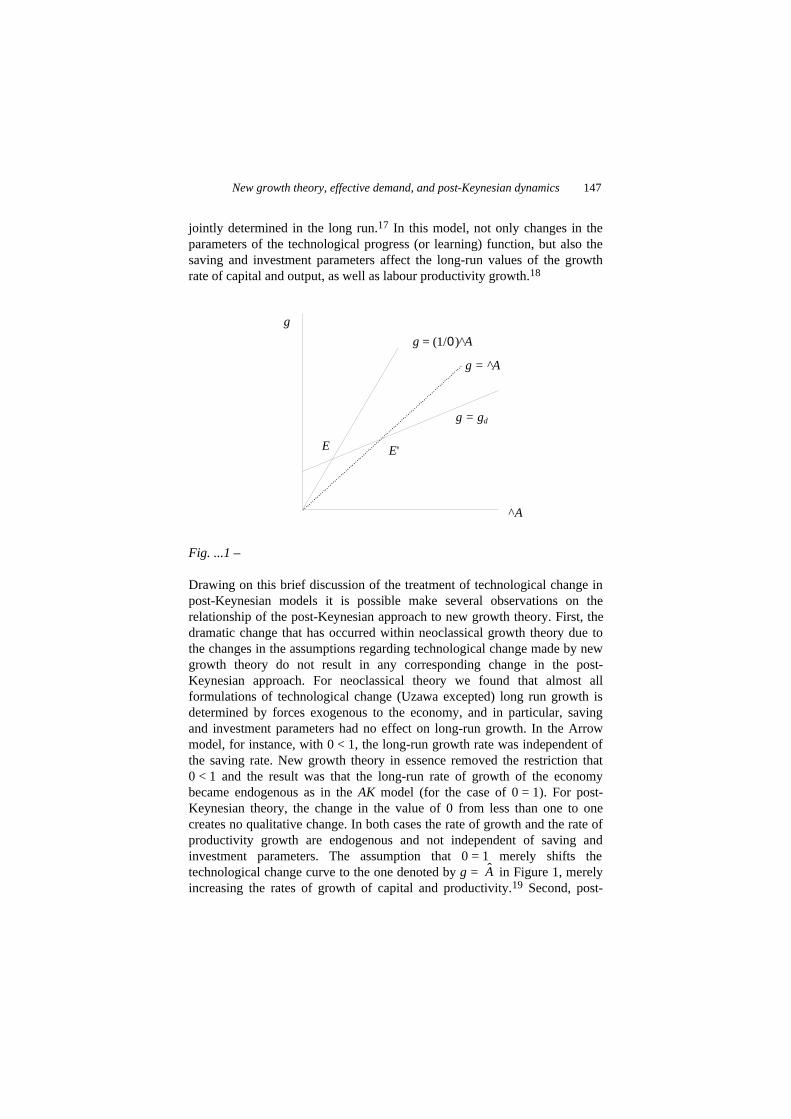
New growth theory, effective demand, and post-Keynesian dynamics 147
jointly determined in the long run.17 In this model, not only changes in the parameters of the technological progress (or learning) function, but also the saving and investment parameters affect the long-run values of the growth rate of capital and output, as well as labour productivity growth.18
g
^A
g = (1/0 )^A
g = ^A
g = gd
E E'
Fig. ...1 –
Drawing on this brief discussion of the treatment of technological change in post-Keynesian models it is possible make several observations on the relationship of the post-Keynesian approach to new growth theory. First, the dramatic change that has occurred within neoclassical growth theory due to the changes in the assumptions regarding technological change made by new growth theory do not result in any corresponding change in the post-Keynesian approach. For neoclassical theory we found that almost all formulations of technological change (Uzawa excepted) long run growth is determined by forces exogenous to the economy, and in particular, saving and investment parameters had no effect on long-run growth. In the Arrow model, for instance, with 0 < 1, the long-run growth rate was independent of the saving rate. New growth theory in essence removed the restriction that 0 < 1 and the result was that the long-run rate of growth of the economy became endogenous as in the AK model (for the case of 0 = 1). For post-Keynesian theory, the change in the value of 0 from less than one to one creates no qualitative change. In both cases the rate of growth and the rate of productivity growth are endogenous and not independent of saving and investment parameters. The assumption that 0 = 1 merely shifts the technological change curve to the one denoted by g = A in Figure 1, merely increasing the rates of growth of capital and productivity.19 Second, post-
148 Old and New Growth Theories: an Assessment
Keynesian growth models with technological change, by allowing aggregate demand to play a major role and incorporating unemployment, have important implications for economic policy regarding saving and investment. New growth theory does not distinguish between saving and investment, and argues that faster growth and technological change requires policies to increase saving and investment. Post-Keynesian models, however, distinguish between the effects of saving and investment parameters: while policies to increase investment can increase growth and technological change, those to increase the saving rate of capitalists can depress aggregate demand and reduce the rate of growth.20 Third, post-Keynesian models, unlike most new growth theory models, imply that not all kinds of technological change will increase the rate of growth of the economy. Post-Keynesian models imply that certain kinds of technological changes, which do not significantly affect investment or consumer demand or industrial structure (which affects the mark-up), are likely to have the primary impact of displacing labour without speeding up growth. By increasing unemployment and depressing aggregate demand, they may in fact have the consequence of slowing down growth. Other kinds of technological changes, which set in motion major changes in investment demand or consumer demand (involving new products and new processes requiring new machines) or shake up industrial structure, thereby having profitability and demand effects, can lead to increases in the rate of growth. This distinction can be said to formalize Baran and Sweezy’s (1966) distinction between ‘normal’ and ‘epoch making’ innovations, a distinction that is not to be found in a qualitative sense in new growth theory models. Fourth, post-Keynesian models can bring into consideration a number of mechanisms of technological change not addressed in new growth theory. For instance, You (1994) makes labour saving technological change depend on labour shortages as captured by the rate of change in the wage, while Lima (1997) examines the interaction between market concentration, industrial innovation and growth in an attempt to synthesize post-Keynesian macrodynamics with evolutionary and neo-Schumpeterian ideas. Freed from the straightjacket of optimization with specific market structures based on market demand based on explicit utility functions that individuals maximize over infinite horizons,21 post-Keynesian models have been able to incorporate arguably more realistic features from stylized facts about actual economies.
Although the discussion so far argues that post-Keynesian models have some advantages over new growth theory models, it would be incorrect to infer that the former can learn nothing at all from the latter. The careful treatment of microfoundations in new growth theory can certainly provide insights from which post-Keynesian growth theories can draw. Rejection of the requirement that all growth models use the dynamic optimization method

New growth theory, effective demand, and post-Keynesian dynamics 149
should not imply that all new growth theory contributions concerning the modelling of firm and innovator behavior should be jettisoned as well. Three issues in particular deserve mention. One, new growth theory models often give careful attention to externalities between firms, taking care to distinguish between firm level variables and economy wide variables (as in the Romer model which distinguishes between private and aggregate capital, although this attention is also to be found in the old neoclassical growth model of Arrow). Post-Keynesian models can do the same, distinguishing more carefully between (say) their own profit rates and aggregate rate of capacity utilization (as an index of the state of the macroeconomy), when they specify behavioural functions which include these variables as arguments. Two, new growth theories derive the values of certain key variables from explicit optimizing decisions, while post-Keynesian models usually take these variables to be exogenously given. Although it is quite legitimate to do this, and perhaps preferable to endogenize these parameters using empirical regularities rather than arbitrary deductive models, it is advisable to check relations based on these regularities against the deductive models. One example is the treatment of the mark-up rate which is often taken to be given and sometimes taken to be a function of other variables such as the rate of technological change in post-Keynesian models, are derived from explicit profit maximizing decisions of firms operating in markets with clearly specified structures. Another example is the treatment of consumer demand parameters from explicit utility functions, which may be particularly useful for the case of the introduction of new products. Three, given the focus of new growth theory on technological change, a great deal of research has been done modelling mechanisms of technological innovation and diffusion, including research and development activities aiming to make profits and education (although the extent to which these contributions are truly new is debatable). Post-Keynesian growth theory can usefully draw on some of these contributions, although not confining attention to only those mechanisms.
....6. CONCLUSION
This paper has examined the contributions of new growth theory from the perspective of post-Keynesian growth theory. Its main conclusions regarding the two theories are as follows.
The advent of new growth theory has resulted in a tremendous resurgence of mainstream growth theory because of its alleged advance over old growth theory by endogenizing the rate of growth of the economy in the long run, making it depend on economic behavior. However, the claims of newness of
150 Old and New Growth Theories: an Assessment
new growth theory for this reason is based on an extremely narrow reading of ‘old’ growth theory that ignores not only some neoclassical contributions but also many non-neoclassical contributions to growth theory. The latter, by allowing for the existence of unemployed labour in the long run, did make long run growth depend on economic behaviour such as investment and saving. Moreover, a careful reading of new growth theory and a comparison with earlier writing on growth and technological change suggests that it has made relatively little progress in terms of addressing new ideas, of developing new ways of modelling macroeconomic dynamics and the mechanisms of technological change, and of understanding the actual growth experiences of capitalist economies regarding productivity changes. Moreover, by assuming away unemployment problems due to the lack of effective demand, it has failed to come to grips with an important feature of the growth process: the integration of medium run macroeconomic phenomenon with long run issues, which are arguably not as separate as is often assumed in mainstream macroeconomic theory.
The paper then presents an alternative to new growth theory in the form of post-Keynesian growth theory, which gives a central place to effective demand and unemployment, and which draws on some of the non-neoclassical contributions to ‘old’ growth theory. It uses this approach to analyze the interaction between technological change and capital accumulation, showing that new growth theory appears far less revolutionary than it claims when seen in terms of this approach, and that while the post-Keynesian approach can learn some things from new growth theory, it can arguably analyze technological change in a more satisfactory way.
We end with two concluding remarks. First, it should be observed that by overemphasizing issues relating to technological change and neglecting effective demand and unemployment, new growth theory diverts attention from other important issues such as financial issues and firm and consumer debt, and their relation to the growth process. Post-Keynesian models have been, and can further be, used to rectify this problem. We have not dealt with this issue here because it is far removed from the concerns of new growth theory (but see Taylor, 1991, for instance). Second, seen from a new growth theory perspective post-Keynesian growth theory may be able to analyze the implications of technological change and financial factors, but only in an ad hoc manner, since it departs from the model of the dynamically optimizing agent. However, this departure may well be an important strength of post-Keynesian growth models which, by breaking free of the straightjacket of implausible dynamic optimizing myths, offers the flexibility to develop simple models incorporating important issues which are relevant for understanding the growth process of actual economies.

New growth theory, effective demand, and post-Keynesian dynamics 151
REFERENCES
Aghion, P. and P. Howitt (1998), Endogenous Growth Theory, Cambridge, Massachusetts: MIT Press.
Ahmad, S. (1966), ‘On the theory of induced innovation’, Economic Journal, 76, 344-57.
Arrow, K.K. (1962), ‘The economic implications of learning by doing’, Review of Economic Studies, 29, 155–73.
Baran, P. and P. Sweezy (1966), Monopoly Capitalism, New York: Monthly Review Press.
Bardhan, P. (1995), ‘The contributions of endogenous growth theory to the analysis of development problems: an assessment’, in J. Behrman and T. N. Srinivasan (eds), Handbook of Development Economics, Vol. 3B, Amsterdam: North Holland.
Bhaduri, A. and S.A. Marglin (1990), ‘Unemployment and the real wage: the economic basis of contesting political ideologies, Cambridge Journal of Economics, 14(4), 375–93.
Dixit, A. (1990), ‘Growth theory after thirty years’, in P. Diamond (ed.), Growth, Productivity and Unemployment, Cambridge, Massachusetts: MIT Press.
Dutt, A.K. (1984), ‘Stagnation, income distribution and monopoly power’, Cambridge Journal of Economics, 8(1), 25–40.
Dutt, A.K. (1990), Growth, Distribution and Uneven Development, Cambridge, UK: Cambridge University Press.
Dutt, A.K. (2001), ‘Kalecki and the Kaleckians: The relevance of Kalecki today’, published in Portuguese, in L. Pomeranz, J. Miglioli and G. Lima (eds), Dinamica economica do capitalismo contemporaneo: Homenagen a M. Kalecki, Sao Paulo: EDUSP, FAPESP.
Fatas, A. (2000), ‘Do business cycles cast long shadows? Short-run persistence and economic growth’, Journal of Economic Growth, 5, June, 147–62.
Harris, D.J. (1978), Capital Accumulation and Income Distribution, Stanford: Stanford University Press.
Hahn, F. and R.M. Solow (1995), A Critical Essay on Modern Macroeconomic Theory, Cambridge, Massachusetts: MIT Press.

152 Old and New Growth Theories: an Assessment
Kahn, R.F. (1959), ‘Exercises in the analysis of growth’, Oxford Economic Papers, 11, 143–56.
Kaldor, N. (1955–56), ‘Alternative theories of distribution’, Review of Economic Studies, 23(2), 61, 83–100.
Kaldor, N. (1957), ‘A model of economic growth’, Economic Journal, 67, 591–624.
Kaldor, N. (1961), ‘Capital accumulation and economic growth’, in F.A. Lutz and D.C. Hague (eds), The Theory of Capital Accumulation, London: Macmillan.
Kaldor, N. (1966), Causes of the Slow Rate of Economic Growth in UK, Cambridge, UK: Cambridge University Press.
Kaldor, N. (1970), ‘The case for regional policies’, Scottish Journal of Political Economy, 18(3), 337–48.
Kalecki, M. (1943), ‘Political aspects to full employment’, Political Quarterly, reprinted in Kalecki (1971).
Kalecki, M. (1971), Selected Essays on the Dynamics of the Capitalist Economy, Cambridge, UK: Cambridge University Press.
Kennedy, C. (1964), ‘Induced bias in innovation and the theory of distribution’, Economic Journal, 74, 541–7.
Keynes, J.M. (1936), The General Theory of Employment, Interest and Money, London: Macmillan.
Kurz, H.D. and N. Salvadori (1995). Theory of Production. A Long-period Analysis, Cambridge: Cambridge University Press.
Kurz, H.D. and N. Salvadori (1998), ‘The “new” growth theory: old wine in new goatskins’, in M. Correlli, M. di Matteo and F. Hahn (eds), New Theories of Growth and Development, London: Macmillan.
Kurz, H.D. and N. Salvadori (1999), ‘Theories of ‘endogenous’ growth in historical perspective’, in R.S. Murat (ed.), Contemporary Economic Issues. Vol 4, Economic Behavior and Design, London: Macmillan in association with International Economic Association.
Lavoie, M. (1992), Foundations of Post-Keynesian Economic Analysis, Aldershot: Edward Elgar.
Lavoie, M. (1995), ‘The Kaleckian model of growth and distribution and its neo-Ricardian and neo-Marxian critiques’, Cambridge Journal of Economics, 19(6), 789–818.

New growth theory, effective demand, and post-Keynesian dynamics 153
Lima, G. (1997), ‘Market concentration and endogenous technological innovation in a model of growth and distributional dynamics’, unpublished, University of Notre Dame, published in Portuguese, in L. Pomeranz, J. Miglioli and G. Lima (eds), Dinamica economica do capitalismo contemporaneo: Homenagen a M. Kalecki, Sao Paulo: EDUSP, FAPESP, 2001.
Lucas, R.E. (1988), ‘On the mechanics of economic development’, Journal of Monetary Economics, 22, 3–42.
Mahalanobis, P.C. (1955). ‘The approach of operational research to planning in India’, Sankhya: Indian Journal of Statistics, 16, 3–62.
Mani, A. (2001), ‘Income distribution and the demand constraint’, Journal of Economic Growth, 6, June, 107–33.
Marglin, S.A. (1984). Growth, Distribution and Prices, Cambridge, Massachusetts: Harvard University Press.
Nelson, R. (1997), ‘What is new in new growth theory?’ Challenge, 40(5), September-October, 29–58.
Ono, Y. (1994), Money, Interest, and Stagnation. Dynamic Theory and Keynes’s Economics, Oxford: Clarendon Press.
Pack, H. (1994), ‘Endogenous growth theory: Intellectual appeal and empirical shortcomings’, Journal of Economic Perspectives, 8(1), Winter, 55–72.
Palley, T.I. (1996), ‘Growth theory in a Keynesian mode: some Keynesian foundations for new endogenous growth theory’, Journal of Post Keynesian Economics, Fall, 19(1), 113–35.
Robinson, J. (1962), Essays in the Theory of Economic Growth, London: Macmillan.
Romer, D. (1996), Advanced Macroeconomics, New York: McGraw Hill.
Romer, P.M. (1986), ‘Increasing returns and long-run growth’, Journal of Political Economy, 94, 1102–37.
Romer, P.M. (1995), ‘Comment’, in T. Ito and A.O. Krueger (eds), Growth Theories in Light of the East Asian Experience, Chicago: University of Chicago Press.
Rowthorn, R. (1982), ‘Demand, real wages and growth’, Studi Economici, 18, 3–54.

154 Old and New Growth Theories: an Assessment
Sen, A. (1970), ‘Introduction’, in A. Sen (ed.), Growth economics, Harmondsworth: Penguin, pp. 9–40.
Skott, P. and P. Auerbach (1995), ‘Cumulative causation and the ‘new’ theories of economic growth’, Journal of Post Keynesian Economics, Spring, 17(3), 381–402.
Solow, R.M. (1956), ‘A contribution to the theory of economic growth’, Quarterly Journal of Economics, 70, 65–94.
Solow, R.M. (1982), ‘Some lessons from growth theory’ in W.F. Sharpe and C.M. Cootner (eds), Financial Economics: Essays in Honor of Paul Cootner, Englewood Cliffs, NJ: Prentice Hall, pp. 246–59.
Solow, R.M. (1988), ‘Growth theory and after’, American Economic Review, 78, 307–17.
Solow, R.M. (1991), ‘Growth theory’, in D. Greenaway, M. Bleaney and I.M.R. Stewart (eds), Companion to Contemporary Economic Thought, London and New York: Routledge, pp. 393–415.
Solow, R.M. (1994). ‘Perspectives on growth theory’, Journal of Economic Perspectives, 8(1), Winter, 45–54.
Solow, R.M. (1997). Learning from ‘Learning by Doing’. Lessons for Economic Growth, Stanford: Stanford University Press.
Srinivasan, T.N. (1995), ‘Long-run growth theories and empirics: Anything new?’ in Ta. Ito and A.O. Krueger (eds), Growth Theories in Light of the East Asian Experience, Chicago: University of Chicago Press.
Steind, J. (1952), Maturity and stagnation in American Capitalism, Oxford: Blackwell.
Taylor, L. (1983), Structuralist Macroeconomics. Applicable Models for the Third World, New York: Basic Books.
Taylor, L. (1991), Income distribution, Inflation and Growth, Cambridge, Massachusetts: MIT Press.
Uzawa, H. (1965), ‘Optimum technical change in an aggregative model of growth’, International Economic Review, 6(1), January, 18–31.
Von Neumann, J. (1945), ‘A model of general equilibrium’, Review of Economic Studies, 13, 1–9.
You, J.-Il (1994). ‘Endogenous technical change, accumulation and distribution’, in A.K. Dutt (ed.), New Directions in Analytical Political Economy, Aldershot: Edward Elgar.

New growth theory, effective demand, and post-Keynesian dynamics 155
NOTES
1. The entire credit for this change does not necessarily lie with new growth theory. A general interest in the problem of economic growth in the West as a result of slow economic growth along with high growth in East Asia certainly had a part to play, as did the appearance of the purchasing power parity adjusted internally comparable data in the form of the Penn Tables. Nevertheless, the nature and direction of the revival of growth economics can largely be explained by the advent of new growth theory.
2. The following analytic history, which concentrates on Harrod’s growth problems and their resolution, is by no means the only one that can be told. An alternative history, suggested by an anonymous referee, underlines the shift from models focusing on production over time, which were related to development planning – when professional communication between classical and neoclassical paradigms was intense, to models of intertemporal consumption efficiency, when there occurred a decisive break between paradigms. While this distinction – and the dogma that the most important requirement of growth models is that individuals optimize utility intertemporally – has constituted the major methodological divide between (old and new) neoclassical growth theorists and heterodox ones, and will be reflected in the following discussion, the history concentrates on Harrod’s problems because they point naturally to the major substantive differences between alternative growth theories and their views of the growth process (for instance, whether growth occurs with full employment or with unemployment), which are the focus of this paper.
3 . Domar’s influential paper, which is bracketed with Harrod’s in the so-called Harrod–Domar model, does not figure prominently in this story, and had an arguably greater influence on early development economics and planning (leading to the emphasis on policies for increasing the saving rate and reducing the capital–output ratio) than on the evolution of growth theory.
4. In presentations of the neoclassical and new growth theory models we will, for simplicity, assume the Cobb-Douglas formulation throughout this paper, except where noted to the contrary. More general constant returns to scale formulations do not change most of the main results, provided E is interpreted as the Harrod–neutral technical progress parameter. One result that it does preclude, however, is the possibility that no steady state may exist in the old neoclassical model due to the violation of the Inada condition, an issue to which we will turn later.
5. The OLG models, however, may not have a stable steady state equilibrium, and may even imply chaotic dynamics.
6. Assuming that the efficiency of labour grows at an exogenously fixed rate will not change the nature of our conclusions.
7. If we wish to allow for population growth, it is easy to check that if equation (12) is replaced by A = K/L, then we will obtain the production function AK for this model, yielding exactly the AK model. In this modified formulation what is relevant for productivity increases is not the stock of knowledge but the stock per unit of labour.
8. This point has been noted earlier by several authors, including Palley (1996) and Kurz and Salvadori (1998), but in my opinion not adequately explored.
9. See Rowthorn (1982) and Dutt (1984) for the original models, and Taylor (1983, 1991), Dutt (1990) and Lavoie (1992) for further analysis.
10. These coefficients are partly determined by technology and partly by social factors such as work practices and organization. A harmless simplification – for our purposes – is to assume that they represent a fixed coefficients, constant returns (Leontief) technology. Since firms are assumed to hire and fire labour according to their demand for worker, we assume that there will never be any excess labour hired by firms beyond what is necessary for

156 Old and New Growth Theories: an Assessment
production; hence the potential and actual labour–output ratio are the same. Since capital, once installed, must be held by firms, they may have excess capacity.
11. A narrow interpretation, based on profit-maximizing models of imperfect competition, can make the mark-up depend solely on the perceived elasticity of demand (assumed constant) of monopolistic competitors, but Kalecki (1971) had a broader interpretation in mind.
12. The rate of capacity utilization can alternatively be measured as the ratio of actual output to potential output, which is Y/(K/a), which is proportional to u, since we assume throughout that the capital-potential output ratio is constant.
13. See Dutt (1990) for a discussion and comparison of these alternative models. 14. Some of alternative models, such as the neo-Marxian one, do not take account of effective
demand considerations explicitly. The foregoing discussion explores how, starting with an analysis which explicitly incorporates the role of effective demand, one can obtain models in which effective demand does not necessarily influence long-run growth in special situations.
15. For a discussion of a number of such models see Dutt (1990) and Taylor (1991) and for a recent survey, see Dutt (2001).
16. It is not possible to assert whether a faster rate of technological change will affect the mark-up positively, negatively or not at all: the direction of change will depend on how technological change affects the various determinants of the mark-up, such as the degree of industrial concentration. Note that that any change in the mark-up is a consequence of a change in the rate of technological change, and such a change is unrelated to the motivations individual firms have of introducing new technology. Technological change, other things constant, increases the profits of the firm which experiences it (and this is sufficient to explain the motivation behind technological change), but these other things may not ultimately be constant due to various systemic consequences (such as changes in industrial concentration).
17. Willy Cortez’s unpublished dissertation written at the University of Notre Dame earlier used this diagram for a related post-Keynesian model.
18. The model discussed here has the property that the saving and investment rates (as a proportion of output) are not positively associated with the rate of growth or the rate of growth of productivity, contrary to the usual empirical evidence which finds that higher saving and investment rates are positively related to growth. This can be seen as follows. The equilibrium saving and investment rates in this model are given by I/Y = S/Y = g/u. Equation (17) implies that g/u = sΦ, which implies that the only parameters that increase the saving and investment rate, that is, s and Φ, also reduce the rate of growth, g. An upward shift in the investment parameters, such as (0, has no effect on the saving and investment rate, although it increases g, because it increases u equiproportionately. This anomaly, however, depends on certain simplifying assumptions of the models. For instance, if the capitalist saving function is given by
S = sΦY – ∃K, with ∃ > 1 to capture the positive effect of wealth in the form of capital on capitalist
consumption, we get g = sΦu – ∃. This implies that g/u = sΦ – ∃/u. An upward shift in the investment function will now increase u and g, but increase g/u and hence the saving and investment rates. Note now, however, that the precise relation between the saving and investment rates and the growth rate depends on what causes changes in both. For instance, contrary to the case of the increase in the investment parameters, an increase in s can increase the saving and investment rates and reduce the rate of growth of the economy.
19. See Palley (1996) for an earlier attempt to develop a synthesis of Keynesian and new growth approaches. This earlier contribution, however, suffers from at least two problems in

New growth theory, effective demand, and post-Keynesian dynamics 157
characterizing both new growth and Keynesian approaches. First, Palley assumes that in old neoclassical growth theory labour productivity growth is exogenous, while in new growth theory it depends, among other things, on the capital-labour ratio. This way of distinguishing old from new growth theory is incorrect, given that old growth theory did endogenize technological change, but generally found it to be exogenous in long run equilibrium. Second, and more importantly for our discussion, the model does not allow effective demand to determine output, which is still determined by a production function in which labour grows at the rate of growth of the exogenously-given supply of labour although capital grows according to investment demand (with the role of saving ignored). Effective demand is introduced into the model by specifying that changes in effective demand growth are caused by deviations of output growth from effective demand growth, and by assuming that the investment rate depends on the growth of effective demand. In the Keynesian framework adopted in the model here, output is determined by effective demand, and both saving and investment functions play a role in determining output and its growth.
20. It should be noted that merely distinguishing between saving and investment functions is not sufficient for allowing effective demand to affect long run growth or for generating unemployment. This should be obvious from the neoclassical Keynesian macroeconomic models of textbooks which produce full employment in the long run with wage flexibility through Keynes (or interest rate) and real balance effects despite their having investment functions, and the neoclassical Keynesian growth model with Tobin’s q. For examples of growth models with separate investment and saving functions which produce supply-determined full employment growth, see Dixit (1990) and Palley (1996).
21. A similar comment can be made about overlapping generations models, which in addition to optimization insert a rigid dynamic framework in which individuals live for two periods.