AA274A: Principles of Robot Autonomy ICourse Notes

Nov 5, 2019

17 Robot Localization

Mobile robot localization is the problem of determining the pose of a robot relative to agiven map of the environment1. It is often called position estimation or position tracking.Mobile robot localization is an instance of the general localization problem, which is themost basic perceptual problem in robotics. This is because nearly all robotics tasks requireknowledge of the location of the robots and the objects that are being manipulated (althoughnot necessarily within a global map).

Localization can be seen as a problem of coordinate transformation. Maps are described ina global coordinate system, which is independent of a robot’s pose. Localization is the processof establishing correspondence between the map coordinate system and the robot’s localcoordinate system. Knowing this coordinate transformation enables the robot to express thelocation of objects of interests within its own coordinate frame—a necessary prerequisite forrobot navigation. As the reader easily verifies, knowing the pose xt = (x, y, θ)T of a robot ina 2D world is sufficient to determine this coordinate transformation, assuming that the poseis expressed in the same coordinate frame as the map.

Unfortunately—and herein lies the problem of mobile robot localization—the pose canusually not be sensed directly. Put differently, most robots do not possess a (noise-free!)sensor for measuring pose. The pose has therefore to be inferred from data. A key difficultyarises from the fact that a single sensor measurement is usually insufficient to determinethe pose. Instead, the robot has to integrate data over time to determine its pose. To seewhy this is necessary, just picture a robot located inside a building where many corridorslook alike. Here a single sensor measurement (e.g., a range scan) is usually insufficient todisambiguate the identity of the corridor.

In this lecture, we will present some basic probabilistic algorithms for mobile localization.All of these algorithms are variants of the basic Bayes filter described in Lecture 14. We willdiscuss the advantages and disadvantages of each representation and associated algorithm.

1Most of this section is a direct excerpt from [TBF05].

1

17.1 A Taxonomy of Localization Problems

Not every localization problem is equally hard. To understand the difficulty of a localizationproblem, we will now discuss a brief taxonomy of localization problems. This taxonomywill divide localization problems along a number of important dimensions pertaining to thenature of the environment and the initial knowledge that a robot may possess relative to thelocalization problem.

Local Versus Global Localization Localization problems are characterized by the typeof knowledge that is available initially and at run-time. The type of localization algorithmused heavily depends on the information available at initialization and during a robot’soperation.

• Position tracking. The initial pose of the robot is known with certainty. This approachassumes that as the robot moves in its environment, the pose error remains relativelysmall and concentrated near the robot’s true pose. The EKF works well for this problembecause it approximates the error using a unimodal (i.e. Gaussian) distribution.

• Global localization. Here the initial pose of the robot is unknown. In this scenario, thebelief distribution is inherently multi-modal as the robot attempts to localize itself. Inthis case, non-parametric filters like histogram or particle filters are preferable.

• Kidnapped robot problem. This problem is a variant of the global localization problem,but one that is even more difficult. During operation, the robot can get kidnappedand teleported to some other location. The kidnapped robot problem is more difficultthan the global localization problem, in that the robot might believe it knows where itis, while in reality, it does not. In global localization, the robot knows that it doesn’tknow where it is. One might argue that robots are rarely kidnapped in practice. Thepractical importance of this problem, however, arises from the observation that moststate-of-the-art localization algorithms cannot be guaranteed never to fail. The abilityto recover from failures is essential for truly autonomous robots. Testing a localizationalgorithm by kidnapping it measures its ability to recover from global localizationfailures.

Static Versus Dynamic Environments Environmental changes are another importantconsideration in mobile robot localization. Environments can be static or dynamic.

• Static environment assumes that the robot is the only object that moves. Put dif-ferently, only the robot moves in a static environment. All other objects in the en-vironment remain at the same location forever. Static environments have some nicemathematical properties that make them amenable to efficient probabilistic estimation.

• Dynamic environments possess objects other than the robot whose locations or config-urations change over time. This problem is usually addressed by augmenting the state

2

vector to include the movement of dynamic entities, or by filtering the sensor data toremove the effects of environment dynamics.

Passive Versus Active Approaches Depending on the application, the localization al-gorithm may or may not control the motion of the robot.

• Passive localization. Passive localization assumes that a single module takes mea-surements, and the robot’s motion is unrelated to its localization process. The robotis controlled through some other means, and the robot’s motion is not aimed at fa-cilitating localization. For example, the robot might move randomly or perform itseveryday’s tasks.

• Active localization. Active localization is more sophisticated. The robot’s movementis aimed (at least partly) toward improving its understanding of the environment. Forexample, a robot in a corner will tend to reorient itself to face the rest of the room,so it can collect environmental information as it moves along the wall. In the samesituation, a passively localized robot may simply slide along with its camera facing thewall. However, since active approaches require control over the robot, they tend to beinsufficient in practice. They are often combined with passive techniques that operatewhen the robot is performing tasks other than localization.

Single Robot Versus Multi-Robot The difficulty of the localization problem also de-pends on the number of robots involved.

1. Single-robot localization is the most commonly studied and utilized approach. Only asingle robot is used in this scheme, and this approach offers the advantage of havingall data collected in a single platform.

2. Multi-robot localization occurs when a team of robots share information in such a waythat one robot’s belief can be used to influence another robot’s belief if the relativelocation between robots is known.

17.2 Localization in Bayesian Filtering Framework

17.2.1 Problem setup

As in the general filtering context, at time t, the state is given by xt, the control inputis given by ut, and the measurements are given by the observation zt. For a differentialdrive robot equipped with a laser range-finder (returning a set of range ri and bearing φimeasurements), we have

xt =

xyθ

ut =

(vω

)zt =

(riφi

)i

. (1)

3

The general strategy for the robot localization problem occurs in two steps: First, duringthe prediction (or action) update, the robot estimates its position through proprioception(such as encoders or dead reckoning) The uncertainty of the robot during this phase increasesdue to the accumulation of odometric error (through integrating over time). The second stepis the perception (or measurement, or correction) update, where the robot uses exteroceptivesensors (such as ultrasonic, laser, camera) to correct its earlier estimated prediction. Theuncertainty of the robot configuration shrinks. By combining these two steps, a robot canlocalize with respect to its map. In order to solve the robot localization problem, the followingingredients are needed:

• Initial probability distribution, bel(x0) for the initial robot location.

• Map of the environment. If not known a priori, then it can be built.

• Data from robotic sensors including the observation zt and the control input ut

• Probabilistic motion model. Derived from robotic kinematics, the current location, x,is a function of previous location, xt, and control input ut, with additional modelederror distributions.

• Probabilistic measurement model. This model is derived from the sensor measurementsof the robot. It consists of the measurement function h depends on the environmentmap and the robot location and an added noise term such that the probability distri-bution peaks at the noise-free value.

17.2.2 Maps

A key ingredient to instantiate Bayes filtering in the context of localization is a map. A mapm is a list of objects in the environment along with their properties, given by

m = {m1,m2, . . . ,mN} (2)

Each mi is an object that encapsulates some property of the environment. The two typesof maps we will focus on here are location-based maps and feature-based maps. As willbe discussed further in the next sections, different map types typically have a trade-off incomputational efficiency and explicitness.

Location-based maps For location-based maps, an index i corresponds to a specificlocation (and hence, they are volumetric). Figure 1 shows two examples of location-basedmaps.

The first example of a location-based map employs vertical cell decomposition. Thismethod essentially sweeps a vertical line through the width of the environment, and everytime a corner is encountered, a cell is built. The result is a set of trapezoidal cells as shown inFig. 1, left. Each element of the map vector would be one of the cells. It is important to notethat this technique can only describe the location of the robot using the presence or absence

4

Figure 1: Two examples of location-based maps.

of the robot in a cell, but cannot give information on where within a cell the robot may be.The second common example of a location-based map uses fixed cell decomposition (Fig. 1,right). In this grid map, the ith element of the map corresponds to the vector xi positionof the i-th cell of the grid map. Thus, each cell represents a map vector. As compared thethe fixed cell decomposition, the vertical cell decomposition is more efficient, as it abstractsthe environment as a graph with nodes and edges. However, fixed cell decomposition canhave better spatial resolution at the expense of additional computational complexity. Bothtechniques can give both the presence and absence of an object, which cannot be done withfeature-based maps.

Feature-based maps For feature-based maps, an index i is a feature index, and mi con-tains, next to the properties of a feature, the Cartesian location of that feature. One canthink of this type of map as a collection of landmarks, such as points or lines. Figure 2 givestwo examples of feature-based maps.

The first example, the lined-based map, uses a line representation of the environment andis commonly used in structured environments like buildings. This is the type of map thatwe will focus on in this class, but the concepts covered on filtering and localization apply toall maps. The second example is the topological map, which, rather than directly measuringgeometric environmental quantities, abstracts the environment as a collection of high levelfeatures. These features could be the position of a chair or a lamp, for example. These typesof abstractions can improve the computational efficiency but feature-based maps cannot giveinformation on the presence and absence of a specific object in the environment.

17.2.3 State Transition

As we have seen previously, the motion model is probabilistic: p(xt|ut, xt − 1) describesthe posterior distribution over the kinematic states that the robot assumes when executingcontrol ut when starting from xt−1. An illustration of this concept is shown in Figure 3.However, unlike what we have seen previously, we introduce the map, which plays a role

5

Figure 2: Two examples of feature-based maps.

in the forward propagation of the dynamics. It is important to note that p(xt|ut, xt − 1) 6=p(xt|ut, xt− 1,m). To understand why, consider the possible future states of the robot whenit is next to a wall. If we do not consider the map, the model may erroneously give a nonzero probability that the robot can travel through the obstacle.

To avoid sampling from the state transition function, which is hard to do, a commontechnique is to make the approximation:

p (xt|ut, xt−1,m) ≈ ηp (xt|ut, xt−1) p (xt|m)

p (xt)(3)

The derivation of this approximation is as follows. Using Bayes theorem,

p (xt|xt−1, ut,m) =p(m|xt, xt−1, ut)p (xt|xt−1, ut)

p(m|xt−1, ut)(4)

Because p(m|xt−1, ut) is independent of xt we can include it in a normalizer, η′, so

p (xt|xt−1, ut,m) = η′p(m|xt, xt−1, ut)p (xt|xt−1, ut) (5)

Now we make the approximation that p(m|xt, xt−1, ut) ≈ p(m|xt), which neglects wherewe are coming from (discarding the information that says along a given motion, we mighthave an obstacle).

p (xt|xt−1, ut,m) = η′p(m|xt)p (xt|xt−1, ut) (6)

The last step involves using Bayes rule again to write p(m|xt) = p(xt|m)p(m)/p(xt).Because p(m) is independent of xt, we can include it in a normalizer: η = η′p(m).

Finally,

p (xt|ut, xt−1,m) ≈ ηp (xt|ut, xt−1) p (xt|m)

p (xt)(7)

6

Figure 3: Probabilistic Motion

η, the normalizing factor, is equal to one divided by the sum of the total probability ofthe rest of expression so that the resulting probability density function sums to 1.

In general, the prior with respect to xt is uniform so the denominator in the final ex-pression also gets included as a constant in the normalizer. Then, the terms that remainare the two probability functions in the numerator. The first is the probability distributionof the future state of the robot as if there were no obstacles. The second is the probabilityof x given m, which is essentially a consistency check that gives the plausibility of a statext given a map. For example, in a grid world representation, the result could be a binaryrandom variable, where the probability that the robot is in the same cell as an obstacle is 0and otherwise the result is 1. This approximation essentially computes the state transitionassuming no obstacles and then applies a consistency check.

Next, we ground the measurement model in the map. The measurement model is prob-abilistic p(zt|xt,m) and we have to condition with respect to a map because the observa-tion also depends on the map. Sensors usually generate more than one measurement whenqueried, so we have batches of measurements zt = {z1t , ..., zKt }. This is the main differ-ence with respect to the Bayes filter (where we were considering sequential measurements).Typically, for simplicity, we assume that these measurements are independent so that

p (zt|xt,m) =K∏k=1

p(zkt |xt,m

)(8)

17.3 Markov Localization

Markov localization uses a specified probability distribution across all possible robot posi-tions. This high level instantiation of the Bayes filter in the context of localization is fairlystraightforward as follows.

We input our belief pose at t − 1 given by bel(xt−1), our control ut, our measurementzt, and the conditioning over the map m. The Markov localization model is conceptuallyidentical to the Bayes filter except for the inclusion of m.

Markov localization has the goal of iteratively propagating forward the belief over thepose of the robot in two steps. The first step is a prediction step that leverages the knowledgeof the state transition function of the robot to go from bel(xt−1) to bel(xt). The second step

7

Figure 4: Markov Localization Algorithm

is the correction step that accounts for the measurement feedback. Figure 4 illustrates anexample of this algorithm.

As is the case for Bayes filters, we must initialize the Markov localization algorithm withan initial belief bel(x0). For position tracking, if the initial pose is known,

bel (x0) =

{1 if x0 = x00 otherwise

(9)

If the initial pose is partially known,

bel (x0) ∼ N (x0,Σ0) . (10)

For global localization, where the initial pose is unknown, the belief is initialized as a uniformdistribution

bel (x0) = 1/|X|. (11)

To make the Markov localization algorithm tractable, we need to add some structure to therepresentation of bel(xt). We can consider three representations. The next section will covera Gaussian representation in the context of EKF localization.

8

Figure 5: Markov Localization Illustration. We consider a robot moving along a wall withthree doors (a) The belief is initialized with a uniform distribution. (b) The robot movesto the first door and makes an observation. We apply the correction step to update ourbelief (c) The robot moves to the second door. The shifted belief is flattened becausethere is uncertainty with how much we moved. (d) We take a second observation, applythe correction, and obtain a large peak in the posterior belief. (e) The robot’s belief aftermoving further down the wall

9

17.4 Extended Kalman Filter (EKF) Localization

The key idea of EKF localization is to represent the belief bel(xt) by its first and secondmoment, µt and

∑t. We will assume that a feature-based map is available, consisting of

point landmarks, given by

m = {m1,m2, . . . ,mN}, mj = (mj,x,mj,y) (12)

where each mj encapsulates the location of the landmark in the global coordinate frame. Wealso assume that we have a sensor that can measure the range r and the bearing φ of thelandmarks relative to the robot’s local coordinate frame.

The range and bearing sensors measure a set of independent features at time t

zt = {z1t , z2t , . . .} = {(r1t , φ1t ), (r

2t , φ

2t ), . . .) (13)

where each measurement zit contains the range rit and bearing φit. We also instantiate amotion model assuming a differential drive robot with states (x, y, θ).

Now that we’ve made assumptions about the map, measurements, and the robot motion,we can instantiate the measurement model which will allow us to re-derive the equationsfor the Markov localization filter. The measurement model tells us the likelihood of a givenmeasurement given our state. Therefore, assuming that the i-th measurement at time tcorresponds to the j-th landmark in the map m, the measurement model is

(ritφit

)= h (xt, j,m) +N (0, Qt) (14)

where N (0, Qt) is the model’s Gaussian noise and

h (xt, j,m) =

( √(mj,x − x)2 + (mj,y − y)2

atan 2 (mj,y − y,mj,x − x)− θ

). (15)

17.4.1 Data Association

The data association problem is the potential uncertainty about the identity of a landmark.For instance, we may be given a range and bearing, but these measurements are not verymeaningful if we do now know what landmark they are given with respect to. As a result,for a map with N total landmarks, we define a correspondence variable cit ∈ 1, ..., N + 1 thatrelates measurement zit and landmark mj, where

• cit = j ≤ N if the i-th measurement at time t corresponds to the j-th landmark

• cit = N + 1 if a measurement does not correspond to any landmark

There are two versions of the localization problem - when the correspondence variables areknown, and when they are not known. We generally only deal with the second case inpractice, but to gain insight, we start by discussing the first version.

10

Figure 6: EKF Localization with Known Correspondences

17.4.2 EKF Localization with Known Correspondences

The EKF localization algorithm is derived from the EKF filter, but with two main differ-ences - measurements are now associated with landmarks, and multiple measurements areprocessed at the same time. We begin again with our differential drive robot and assump-tion of the stochastic motion model (with some process disturbance ε that has a Gaussiandistribution) and Jacobian G:

xt = g (ut, xt−1) + εt, ε ∼ N (0, Rt) , Gt := Jg (µt, µt−1) (16)

The (nonlinear) range and bearing measurement model h(xi, j,m) now includes the index jof the landmark with respect to which we are taking the measurements:

zit = h (xi, j,m) + δt, δt ∼ N (0, Qt) , H it :=

∂h(µt,j,m

)∂xt

(17)

Here δ is again the measurement noise, and H is the measurement Jacobian. From differen-tiating 15,

Qt =

(σ2r 0

0 σ2φ

)(18)

11

The EKF localization algorithm is shown below. The key differences from the Bayes/EKFfilter are the new inputs (the correspondence variables ct and map m), and the fact thatwe are now considering batches of measurements. As with the Bayes filter, we start withthe prediction step, in which the mean and variance are propagated using Taylor seriesexpansions. We then carry out the correction step by exploiting the conditional independenceassumption for our batch of measurements,

p (zt|xt, ct,m) =∏i

p(zit|xt, cit,m

)(19)

which allows us to incrementally add information (i.e. process the measurements sequen-tially) as if there was no motion between measurements.

The EKF-localization steps are illustrated for a differential drive robot in the Figure 7,8and 9. Implementation details are outlined in Figure 6.

Figure 7: The prediction step. Observations measure the relative distance (range) andheading (bearing) of the robot to a landmark. We assume here that the robot detects onlyone landmark at a time.

12

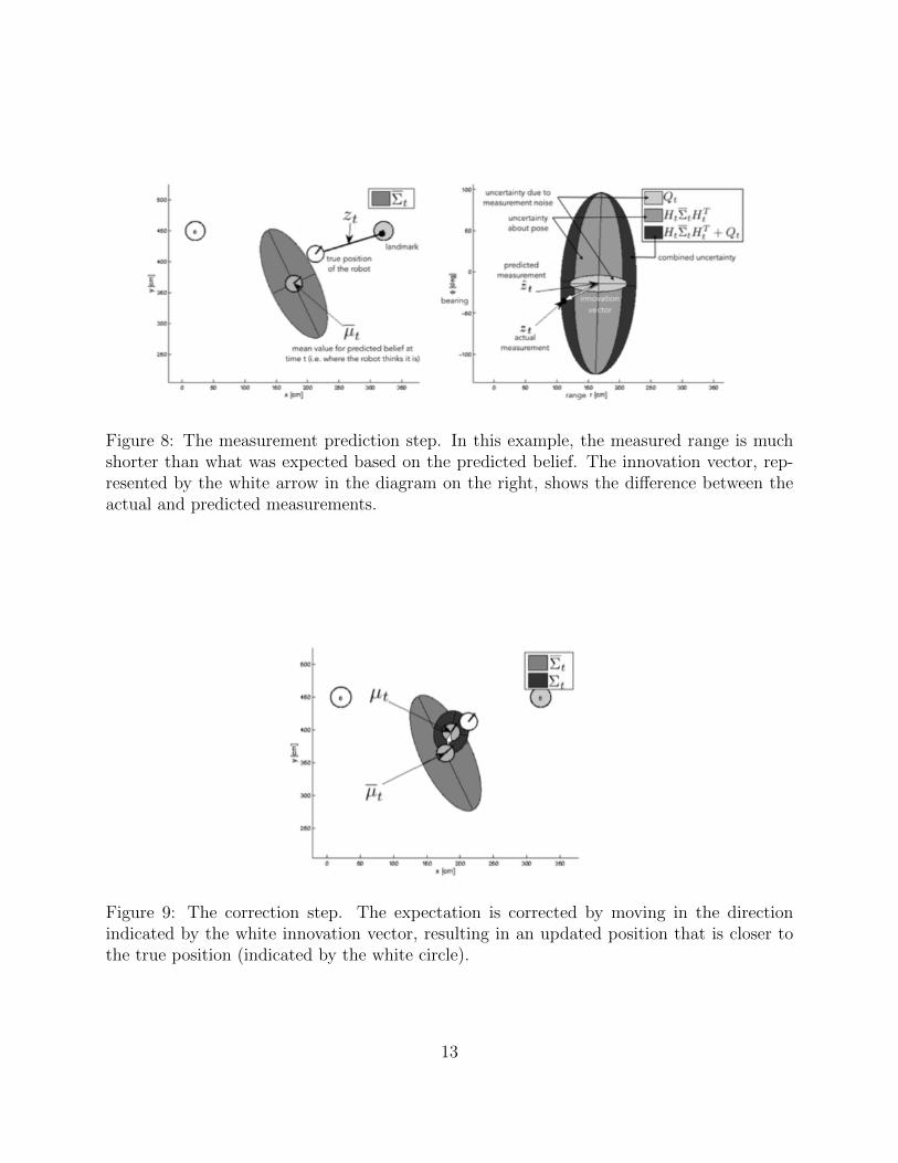
Figure 8: The measurement prediction step. In this example, the measured range is muchshorter than what was expected based on the predicted belief. The innovation vector, rep-resented by the white arrow in the diagram on the right, shows the difference between theactual and predicted measurements.

Figure 9: The correction step. The expectation is corrected by moving in the directionindicated by the white innovation vector, resulting in an updated position that is closer tothe true position (indicated by the white circle).

13

Figure 10: EKF Localization with Unknown Correspondences Algorithm

17.4.3 EKF Localization with Unknown Correspondences

For EKF localization with unknown correspondences, we must jointly estimate the corre-spondence variables and use these estimates to implement the Markov filter. The simplestway to determine the identity of a landmark during localization is to use maximum likeli-hood estimation, in which the most likely value of the correspondences ct is determined bymaximizing the data likelihood:

ct = arg maxct

p (zt|c1:t,m, z1:t−1, u1:t) (20)

In other words, we pick the set of correspondence variables that maximizes the probabilityof getting the measurement that we see, given the history of correspondence variables, themap, the history of measurements, and the history of controls. The value of ct is then takenfor granted, so this method can be quite brittle; any mistake made during this process willpropagate into the future.

The challenge with this method is that each element can take on many values (equal tothe number of landmarks), and the number of possible combinations is exponential. Theoptimization problem is therefore over an exponentially large physical space for a nonlinearfunction. As a result, we must resort to applying reasonable approximations with a modelof independent measurements, and perform maximization separately for each zit. Imple-mentation details of EKF Localization with unknown correspondences is outlined in Figure10.

14

17.4.4 Estimating the Correspondence Variable

The first step to solving the set of correspondence variables is to optimize the correspondencevariables one by one:

p(zit|c1:t,m, z1:t−1, u1:t

)(21)

Essentially, we want to find the likelihood of zit given the conditions at c, m, z, and u. In orderto do so, we use the total probability theorem. Through this method, we are optimizing thelikelihood of each individual event instead of a joint optimization of all likelihood events atonce. After algebraic manipulation, this translates to performing the following calculation:

p(zit|c1:t,m, z1:t−1, u1:t

)≈ N

(h(µt, c

it,m

), H i

tΣt

[H it

]T+Qt

)(22)

What we get is that the probability of zit is approximately equal to the Gaussian distributionwith mean equal to the predicted measurement. The next step is to find the correspondencesusing this Gaussian distribution with the following estimation:

cit = argmax p(zit|c1:t,m, z1:t−1, u1:t

)≈ argmaxN

(zit;h

(µt, c

it,m

), HtΣtH

Tt +Qt

)(23)

For EKF with unknown correspondences, we apply an algorithm very similar to the onefor EKF localization with known correspondences. The new algorithm includes a maximumlikelihood estimator for the correspondence variables, as we are now no longer assumingthe correspondence variables are inputs but rather optimizing for their values. The generaloutline of the algorithm is to do prediction, estimation, correspondences between measure-ments and landmarks, and finally correction. Examples of some common landmarks arelines, corners, and distinct patterns.

References

[TBF05] Sebastian Thrun, Wolfram Burgard, and Dieter Fox. Probabilistic robotics. MITpress, 2005.

15