a3dadaptivemeshmovingschemeamasud.web.engr.illinois.edu/papers/kanchi-masud-ijnmf-2007.pdf924 h....

INTERNATIONAL JOURNAL FOR NUMERICAL METHODS IN FLUIDSInt. J. Numer. Meth. Fluids 2007; 54:923–944Published online 1 May 2007 in Wiley InterScience (www.interscience.wiley.com). DOI: 10.1002/fld.1512

A 3D adaptive mesh moving scheme

Harish Kanchi1,‡ and Arif Masud2,∗,†,§

1Department of Mechanical Engineering, University of Illinois at Chicago, Chicago, IL 60607, U.S.A.2Department of Civil and Environmental Engineering, University of Illinois at Urbana-Champaign,

Urbana, IL 61801, U.S.A.

SUMMARY

This paper presents an adaptive mesh moving technique for three-dimensional (3D) fluid flow problemsthat involve moving fluid boundaries and fluid–solid interfaces. Such mesh moving techniques are anessential ingredient of fluid–structure interaction methods that typically employ arbitrary Lagrangian–Eulerian (ALE) frameworks. In the ALE frame, the velocity field representing motion of the underlyingcontinuum is integrated in the fluid flow equations. In the discretized setting, the velocity field of theunderlying continuum gives rise to the mesh displacement field that needs to be solved for in additionto the flow equations and the structural equations. Emphasis in the present work is on the motion anddeformation of 3D grids that are composed of linear tetrahedral and hexahedral elements in structuredand unstructured configurations. The proposed method can easily be extended to higher-order elementsin 3D. A variety of moving mesh problems from different fields of engineering are presented that showthe range of applicability of the proposed method and the class of problems that can be addressed withit. Copyright q 2007 John Wiley & Sons, Ltd.

Received 27 December 2006; Revised 20 March 2007; Accepted 21 March 2007

KEY WORDS: mesh moving scheme; fluid–structure interaction; moving boundary flows; 3D meshes

1. INTRODUCTION

In the modelling of fluid–structure interaction (FSI) problems, one needs to write the flow equationsin an arbitrary Lagrangian–Eulerian (ALE) frame of reference wherein the underlying physicaldomain can move and deform independently of the motion of the fluid particles (see e.g. [1–4] andreferences therein). This class of problems can also be addressed via the space–time finite element

∗Correspondence to: Arif Masud, Department of Civil and Environmental Engineering, University of Illinois atUrbana-Champaign, Urbana, IL 61801, U.S.A.

†E-mail: [email protected]‡Graduate Research Assistant.§Associate Professor of Mechanics and Structures.

Contract/grant sponsor: Office of Naval Research; contract/grant number: N000014-00-1-0687

Copyright q 2007 John Wiley & Sons, Ltd.

924 H. KANCHI AND A. MASUD

approaches wherein the space–time finite element slabs are oriented in time to accommodatethe spatial deformation of the computational grids. Space–time methods for FSI problems wereproposed by Tezduyar and coworkers [5–9] and by Masud [10] and Masud and Hughes [11].An equivalence between the ALE-based methods and slanted space–time methods for FSI wasformally established in [10, 11].

In coupled solution strategies for FSI problems, an essential ingredient is the ability to movethe fluid mesh nodes to accommodate the deformation of the time-dependent physical boundariesand at the same time maintain the quality of the computational grids for successive time-stepcalculations. From the viewpoint of computational efficiency, the mesh moving scheme shouldyield a good fluid mesh with the least amount of computational expense. For a review of thevarious recent approaches for mesh motion, see e.g. [5, 6, 12–22] and references therein.

In Masud et al. [4], we presented a 2D adaptive mesh moving scheme for structured andunstructured meshes. Various mesh types comprising linear triangular and quadrilateral elementswere tested for a range of physical problems from various fields of engineering. The algorithm wasintegrated in a multiscale/stabilized formulation for the incompressible Navier–Stokes equationsfor 2D moving boundary flows [3, 23]. In [24], it was shown that an arbitrary motion of thecomputational grid can potentially induce instability in the numerical computations and it wassuggested that the mesh motion should be such that it also minimizes the local relative velocity.

Present paper presents an extension of the 2D scheme to 3D, and emphasis is on large-scalemeshes of industrial strength. Like the 2D case presented in [4], the present formulation accom-modates different 3D element types in the same computational domain which is a very attractivefeature from practical problem solving viewpoint. An outline of the paper is as follows. Section 2presents the boundary value problem for mesh motion that gives rise to a modified variational formthat prevents the inversion of smaller elements in the boundary layer region. Numerical experi-ments with linear hexahedral and tetrahedral elements are presented in Section 3 and concludingremarks are presented in Section 4.

2. THE MODIFIED EQUATION FOR MESH MOTION

We indicate the computational fluid domain by � where � ⊂ Rnsd is a bounded open set withpiecewise smooth boundary �; nsd = 3 denotes the number of spatial dimensions. We indicate themoving and fixed parts of the boundary via �m and �f, respectively. The boundary � admits thefollowing decomposition:

�= �m ∪ �f (1)

and

�=�m ∩�f (2)

In Masud et al. [4], we proposed a modified equation for mesh rezoning that was designed to movethe finer zones of the mesh that usually lie in the boundary layer regions, with least amount ofdistortion. To achieve this end, the weak form of Laplace equation for mesh motion is modified byadding to it a least-square term. The formal statement of the boundary value problem for the mod-ified equation is: given g, the prescribed mesh displacement at the moving boundary, find the mesh

Copyright q 2007 John Wiley & Sons, Ltd. Int. J. Numer. Meth. Fluids 2007; 54:923–944DOI: 10.1002/fld

A 3D ADAPTIVE MESH MOVING SCHEME 925

displacement field u : � → Rnsd , such that

∇ · ([1 + �]∇)u= 0 (3)

u= g on �m (4)

u= 0 on �f (5)

Equations (3)–(5) represent the governing equation, the moving, and the fixed boundary conditions,respectively. Spaces relevant to the boundary value problem are

S ={u | u∈ (H1(�))nsd, u= g on �m and u= 0 �f} (6)

V = {w |w∈ (H10 (�))nsd} (7)

where H1(�) denotes the space of functions in L2(�) with generalized derivatives also in L2(�).H10 (�) is a subset of H1(�), whose members satisfy zero boundary conditions.In order to understand the role of � in Equation (3), consider a typical unstructured and a

graded fluid mesh. Such meshes have local refinement in the regions of boundary layers to capturethe small-scale effects. For FSI problems involving moving boundaries, objective is to move thesmaller elements in the boundary layers together with the interfaces with the least amount ofdistortion so as to attain well-conditioned meshes for subsequent time steps. This is achieved viaimposing the constraint condition over the elements that effectively introduces additional stiffnessin the element which is inversely proportional to the relative size of the element in the mesh [4].To understand the role of the constraint condition, consider a 2-node linear element with nodes iand j , and the nodal displacements at the nodes indicated by uhi and uhj , respectively. Goal is tolimit the relative difference in the value of the displacement field at the two nodes to be less thanthe element length he, i.e.

|uhi − uhj |��he (8)

⇒ |∇uh |�� (9)

where he is the length of the element, and � ∈ [0, 1) is a tolerance parameter for element distortion.Consequently, the case of least distortion in smallest elements is attained in the limit as � → 0,namely, for multidimensional case,

∇uh = 0 (10)

This condition can be applied element wise, and consequently leads to a modification of theunderlying Laplace equation typically used for mesh moving. The constraint is imposed in aweighted form thereby introducing the function � in (3). In the discrete setting, this gives riseto the element-based weight function �e which is a non-dimensional and positive function in �e.This bounded, non-dimensional function is designed such that it imposes condition (10) ratherstrictly over the smaller elements as compared to that over the larger elements, thus introducinga stiffening effect that is inversely proportional to the size of the elements. This spatially varyingstiffening effect causes the mesh to deform non-uniformly by translating most of the deformationto the larger elements in the mesh that usually lie in the far field region.



2.1. Design of the weight function for mesh motion

A simple definition of the discrete �e proposed in Masud and Hughes [11] is

�e = 1 − Vmin/Vmax

V e/Vmax(11)

In the context of 3D elements, V e, Vmax and Vmin represent the volumes of the current, the largestand the smallest elements in a given mesh, respectively. The plot shown in Figure 2 is the variationof this weighting function with respect to the ratio of the volume of the current element andthe volume of the largest element in a 3D hexahedral fluid mesh shown in Figure 1. This trendis similar to that for the 2D case as presented in [4]. Because of the spatially varying stiffnessintroduced in the fluid mesh, the elements adjoining the moving boundaries or the solid–fluidinterface boundaries translate with the interface with the least amount of distortion, while thedeformation is largely accommodated by the larger elements that behave relatively soft and areusually located in the far fields.

Remarks

1. In our simulations, we have used an automatic control on the change in the condition numberof the element by comparing the Jacobian of the element in the current (deformed) mesh withits corresponding value in the initial (undeformed) mesh. In our calculations, if the currentJacobian for a given element is either smaller or larger than a specified percentage of itscorresponding value in the initial undeformed mesh, the calculations are frozen in time anda new mesh is constructed around the current location of the bodies.

2. Ideas stemming from the definition of well-conditioned elements in terms of the side lengthsand interior angles of their underlying reference elements can be brought into play via atensor representation of the weight function �. We will explore these ideas in our subsequentwork.

2.2. The finite element form

Let Sh and V h represent the finite-dimensional subspaces of S and V , respectively, that involvepiecewise polynomial interpolations. The finite element form can be expressed as: find uh ∈ Sh

such that for all wh ∈ V h

B(wh,uh) = L({wh}) (12)

where the bilinear form is

B(wh, uh) = (∇wh,∇uh) +nel∑

e=1�e(∇wh, ∇uh)�e (13)

RemarkA salient feature of this formulation is that standard 3D Lagrange shape functions can be employedin (13) and they will yield a stable method.



3. NUMERICAL EXPERIMENTS

The formulation has been implemented for 3D linear tetrahedral and hexahedral elements. Fullquadrature is employed for numerical integration. For linear tetrahedral elements, the derivatives ofthe shape functions are constants and therefore one-point integration suffices for the calculation ofthe element stiffness matrix. Hexahedral elements on the other hand employ 2× 2× 2 integrationrule. Since the volume of one hexahedral element can be divided into six non-overlapping tetrahedralelements, the cost of computation of system tangent matrix with an equivalent brick mesh that canbe obtained by keeping the number of nodes constant between the two mesh types, is comparable.However, the tetrahedral elements lead to a smaller band width, and therefore considerable savingsin the solution of the problem for mesh displacement field can be attained. Besides, from a practicalviewpoint it is easy to discretize 3D domains via tetrahedral elements than via hexahedral elements.

In the following section, we present example problems from various fields of fluid mechanicsthat involve moving and deforming boundaries. Sections 3.1 to 3.3 present relatively simpler 3Dproblems that are designed with the aim of verifying the proposed method by comparing theoriginal and the deformed mesh configurations. Sections 3.4 to 3.8 present problems from variousindustrial level applications.

3.1. Flexible deformation of multiple cylinders in an unstructured hexahedral mesh

The first test case is that of three flexible cylinders in the fluid domain. This is an example fromthe domain of heat transfer problems where cooling fluid flows around the flexible pipes. The 3Dmesh (showing only the surface mesh) of the cylinder-block model is shown in Figure 1. Meshhas 7824 nodes and 5240 elements. Only four of the six faces are given prescribed zero boundarydisplacement. The faces containing the intersections with the cylinders are free to move and evolvein their respective planes. The three cylinders are given prescribed deflection and translation viafunctions g1i , g

2i and g3i , respectively (see Equation (14)), where i = 1, 2 is the X and Y spatial

dimension; A0i and B0i are given constants; Lz is the length of the cylinder, and x3 representsthe coordinate of the nodal points along the length of the cylinder. The nodes are constrained tomove in the x3 direction. The first and third cylinder move in phase and the middle cylinder moveswith a lag of 180◦. Figure 2 shows the variation of �e with respect to the ratio of the volumeof the current element and the volume of the largest element in the mesh shown in Figure 1.Configurations of the mesh at various time levels are shown in Figures 3–5.

Ai (X) = A0i sin(�x3/Lz) + B0i

g1i (X, t) = g3i (X, t) = Ai (X) sin(4�t)

g2i (X, t) = Ai (X) sin(4�t + �)

g3(X, t) = 0

(14)

3.2. Flexible deformation of multiple cylinders in an unstructured tetrahedral mesh

As the geometric configuration of the computational domain gets intricate, the generation of astructured mesh comprising hexahedral elements becomes a challenging task. In such situations,tetrahedral elements are typically employed because they provide considerable flexibility in meshgeneration around complex geometric shapes. Furthermore, the element stiffness matrix (for mesh



X

Y

Z

Figure 1. Unstructured hexahedral mesh with three flexible cylinders.

V/Vmax

τ

0 0.1 0.2 0.30

100

200

300

400

500

Figure 2. Weighting function � for the hexahedral mesh shown in Figure 1.



X

Y

Z

Figure 3. Spatial configuration of the flexible cylinders at t = 0.8 s.

X

Y

Z

Figure 4. Top view of the mesh showing deflections and translations in XY plane at t = 0.3 s.

motion part of the problem) for linear tetrahedral elements can be computed via one-point integra-tion (because it is composed of constant strain–displacement matrices) and this can considerablyeconomize computations.

The problem description of the current test case is same as that in Section 3.1, and the cylindersare moved with prescribed motion given in (14). Figure 6 shows the unstructured mesh of 4-node



X

Y

Z


X

Y

Z

Figure 6. Unstructured tetrahedral mesh of three flexible cylinders.

tetrahedra containing 9132 nodes and 43 648 elements. The weighting function � as a function ofthe ratio of element size for this mesh is shown in Figure 7. Figures 8 and 9 show the side andtop views of deflection and translation of the flexible cylinders.



V/Vmax

τ

0 0.1 0.2 0.30

100

200

300

400

500

Figure 7. Weighting function � for the tetrahedral mesh shown in Figure 6.

X

Y

Z

Figure 8. Spatial configuration of the flexible cylinders at t = 0.3 s.



X

Y

Z


3.3. Free oscillation of a sphere in an unstructured tetrahedral mesh

This test case is designed to check the performance of the proposed method on the motion ofinterfaces that are completely embedded in the surrounding fluid domain. The mesh around thesphere contains 5861 nodes and 30 930 linear tetrahedral elements. The surface mesh on the sphereand the boundary mesh of the computational domain is shown in Figure 10. The sphere is givena prescribed sinusoidal motion in the YZ plane. The simulation of the mesh motion is shown inFigure 11, where three superposed frames show the positions of the sphere at various instantsduring motion.

3.4. Aerodynamic applications: YF-17 jet simulations

Figure 12 shows a typical mesh around geometric configuration of YF-17 jet. The mesh is composedof 97 104 nodes and 528 925 elements. The definition of �e used for simulations with brick andtetrahedral elements works well for meshes that have up to three orders of mesh refinement. Fortypical industrial applications as shown in Figure 12, there is six orders of magnitude difference inthe sizes of the largest and the smallest elements. For such highly graded meshes, the definition of�e given in (11) leads to a very high numeric value for the elements in the boundary layer region(see, e.g. Figure 13). This causes ill-conditioning in the system tangent matrix, thus causing meshlocking that leads to zero mesh displacements. This locking effect can be seen at the tip of thewing and the tail in Figure 14. In order to avoid locking, we put a limit on the numeric value of�e. Our numerical tests have indicated that if we limit V e

limit = 0.1× Vmax then value of �e givenby (11) does not result in ill-conditioning of the tangent matrix for mesh motion.

3.4.1. Aerodynamic application: YF-17 rolling motion. The mesh motion simulations for theYF-17 jet were carried out using the new definition for �e. The rolling motion is simulatedby rotating the nodes along the longitudinal axis of the plane. Figure 15 shows two superposedframes for two different rotated positions.



XY

Z

Figure 10. Tetrahedral mesh around a sphere.

X Y

Z

Figure 11. Multiple superimposed frames showing the motion of the submerged sphere.



Figure 12. Surface mesh of YF-17 jet configuration.

V/Vmax

τ

0 0.25 0.5 0.75 10

10

20

30

40

50

Figure 13. Value of �e as a function of non-dimensionalized volume of elements for the aircraft mesh.



Figure 14. Mesh locking at the tips of wing and the tail.

XY

Z

Figure 15. Two superimposed frames showing the rolling motion of the jet.

3.4.2. Pitching motion of the jet around its centre of gravity. This simulation is pitching motionof the jet about its centre of gravity. Such simulations are presented by Farhat and coworkers [25].The nodes of the jet are moved around its centre of gravity with a sinusoidal motion in XZ plane.The simulation of the jet at various instants is shown in Figures 16–18.



Figure 16. Surface mesh on the jet.

Figure 17. A representative configuration during the pitching motion.

3.4.3. A method to reduce the cost of computation. In fluid–structure interaction problems, thereare situations where it is important to move the mesh in the boundary layers together withthe solid interfaces with virtually no distortion. This typically happens when the submergedstructure undergoes large translations and rotations, but the mechanical strains in the structure



Figure 18. A later configuration during the pitching motion.

are small. Since in unstructured and graded meshes, elements are invariably clustered aroundthe moving interfaces, so moving these elements in a glued fashion can serve two purposes:(i) it can help in maintaining the quality of grid in the boundary layers for subsequent timestep calculations, and (ii) it can help in reducing the size of the mesh motion problem. Forthe nodes that lie in the glued region, the equations governing the mesh motion are not solved.Rather the location of nodes is updated based on the prescribed displacement dictated by rigid-body motion of the body, thus considerably reducing the number of equations to be solved.One easy way to accomplish this is to create an imaginary box around the structure and thenmoving the entire boxed region with the prescribed motion dictated by rigid-body motion of theconfining structure. Similar ideas where automatic mesh moving technique has been combined withstructured layers of elements undergoing rigid-body motions or deforming like a solid extension ofthe interface have been pursued by Hughes et al. [2], Masud and Hughes [11], Nkonga [18], andTezduyar [8, 26].

In the case of YF-17 jet, we create and imaginary box with length equal to twice the dimensionsof the plane. This causes 43 432 nodes around the jet to have a prescribed motion as compared to9772 nodes when prescribed motion is only applied on to the surface of the jet. The computationaltime required for the two cases on a 2 GHz single processor PC is shown in Figure 19. Fromthis graph it is seen that for the 10 steps used to solve the problem, there is approximately 40%reduction in the time at every step in the case of the glued layered method.

3.5. Rotational motion of a submarine propeller

This simulation represents the class of FSI problems where parts of the mesh are in relative slidingmotion [27, 28]. The current problem is of interest in marine engineering where FSI couplingeffects are produced by rotating propellers that provide the necessary thrust for the propulsionof submarines and surface ships. Rotation of propellers in surrounding fluids is typically solved



0

200

400

600

800

0 3 6 9 12

Time Steps

CP

U t

ime

(sec

)Block Moving

YF-17 Moving

Figure 19. Comparison of CPU times.

Y

Z X

Figure 20. Tetrahedral mesh for submarine FSI problem.

by generating a sequence of fluid meshes that rotate with the propeller and therefore distortand shear with time. In these simulations when elements in one mesh get excessively sheareda new mesh is generated and the flow field is projected onto the new mesh using projectiontechniques. In this work, we advocate the idea of dividing the computational domain into twoparts with the following characteristics: (i) one part of the domain that is in the form of acylinder that encompasses the propeller and thus rotates together with the propeller, and (ii) thesecond part that discretizes the remaining region. This non-overlapping discretization leads to the



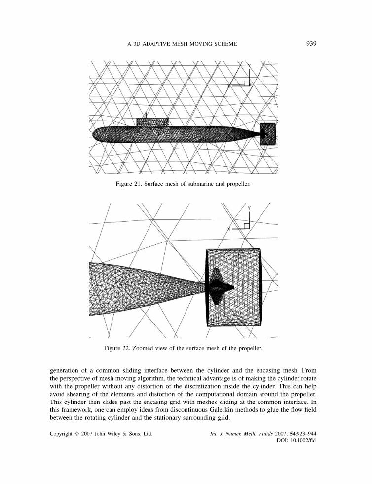
Figure 21. Surface mesh of submarine and propeller.

Figure 22. Zoomed view of the surface mesh of the propeller.

generation of a common sliding interface between the cylinder and the encasing mesh. Fromthe perspective of mesh moving algorithm, the technical advantage is of making the cylinder rotatewith the propeller without any distortion of the discretization inside the cylinder. This can helpavoid shearing of the elements and distortion of the computational domain around the propeller.This cylinder then slides past the encasing grid with meshes sliding at the common interface. Inthis framework, one can employ ideas from discontinuous Galerkin methods to glue the flow fieldbetween the rotating cylinder and the stationary surrounding grid.



Figure 23. Zoomed view of the position of the propeller.

Figure 24. Zoomed view of the rotated propeller at a later instant.



Figure 25. Two superimposed frames showing the relative rotation of the propeller.

Figure 26. Unstructured tetrahedral mesh of the heart.



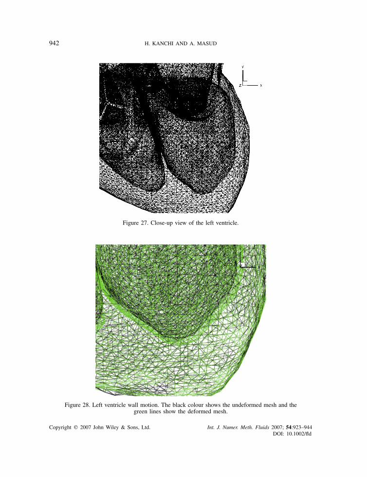
Figure 27. Close-up view of the left ventricle.

Figure 28. Left ventricle wall motion. The black colour shows the undeformed mesh and thegreen lines show the deformed mesh.



Figure 20 shows the surface mesh on the submarine and the bounding surface of the com-putational domain, while Figure 21 shows the close-up view of the longitudinal profile of thesubmarine. The unstructured tetrahedral mesh contains 19 510 nodes and 105 664 elements. Thepropeller model is meshed containing 14 892 nodes and 81 226 elements. These two meshes arecombined and the propeller nodes are given rotational motion, with the rest of the mesh kept sta-tionary. Figure 22 shows a close view of the cylinder where the surface mesh around the propellercan clearly be seen. The simulation of the rotating propeller at different time steps is shown inFigures 23 and 24. Figure 25 shows two configurations of the rotating mesh by superimposing therotated propeller configurations.

3.6. Bio-fluid application: Beating heart simulation

This is a FSI problem from the domain of bio-fluid dynamics and simulates the beating of heart.The mesh has 148 516 nodes and 728 321 elements [29, 30]. The nodes of the atriums are given asinusoidal motion while the ventricles are given a motion which lags 180◦ to that of the atriums.The heart mesh is shown in Figure 26. Figure 27 shows the close-up view of the left ventricle andthe surface mesh for the chamber together with the superimposed outer surface mesh. Figure 28shows the left ventricle of the heart, where undeformed and deformed meshes are superimposedto show the beating of the heart.

4. CONCLUSIONS

We have presented an adaptive mesh moving technique for three dimensional structured andunstructured grids that are composed of linear tetrahedral and hexahedral elements. This methodcan be extended to higher order elements in 3D. Representative examples from different fields ofengineering show the range of applicability of the proposed method.

ACKNOWLEDGEMENTS

This work was partially supported by Office of Naval Research Grant N000014-00-1-0687. This supportis gratefully acknowledged. Authors also wish to acknowledge the following individuals and organizationsfor two of the meshes used here. The mesh for the YF-17 was provided by Dr. A. Coutinho, Departmentof Civil Engineering, COPPE/Federal University of Rio de Janeiro. The mesh for the heart was providedby Dr Y. Zhang, Institute for Computational Engineering and Sciences at University of Texas, Austin.

REFERENCES

1. Donea J. Arbitrary Lagrangian–Eulerian finite element methods. In Computational Methods for Transient Analysis,Belytschko T, Hughes TJR (eds). North-Holland: Amsterdam, 1983; 473–516.

2. Hughes TJR, Liu WK, Zimmerman TK. Lagrangian–Eulerian finite element formulation for incompressibleviscous flows. Computer Methods in Applied Mechanics and Engineering 1984; 29:329–349.

3. Khurram R, Masud A. A multiscale/stabilized formulation of the incompressible Navier–Stokes equations formoving boundary flows and fluid–structure interaction. Computational Mechanics 2006; 38(4–5):403–416.

4. Masud A, Bhanabhagvanwala M, Khurram RA. An adaptive mesh rezoning scheme for moving boundary flowsand fluid–structure interaction. Journal of Computers and Fluids 2007; 36:77–91.

5. Johnson AA, Tezduyar TE. Simulation of multiple spheres falling in a liquid-filled tube. Computer Methods inApplied Mechanics and Engineering 1996; 134:351–373.



6. Mittal S, Tezduyar TE. A finite element study of incompressible flows past oscillating cylinders and airfoils.International Journal for Numerical Methods in Fluids 1992; 15:1073–1118.

7. Tezduyar TE, Behr M, Liou J. A new strategy for finite element computations involving moving boundaries andinterfaces—the deforming-spatial-domain/space–time procedure: I. The concept and the preliminary numericaltests. Computer Methods in Applied Mechanics and Engineering 1992; 94:339–351.

8. Tezduyar TE. Stabilized finite element formulations for incompressible flow computations. Advances in AppliedMechanics 1992; 28:1–44.

9. Tezduyar TE, Behr M, Mittal S, Liou J. A new strategy for finite element computations involving movingboundaries and interfaces—the deforming-spatial-domain/space–time procedure: II. Computation of free-surfaceflows, two-liquid flows, and flows with drifting cylinders. Computer Methods in Applied Mechanics andEngineering 1992; 94:353–371.

10. Masud A. A space–time finite element method for fluid–structure interaction. Ph.D. Thesis, Stanford University,1993.

11. Masud A, Hughes TJR. A space–time Galerkin/least-squares finite element formulation of the Navier–Stokesequations for moving domain problems. Computer Methods in Applied Mechanics and Engineering 1997;146:91–126.

12. Bottasso CL, Detomi D, Serra R. The ball-vertex method: a new simple spring analogy method for unstructureddynamic meshes. Computer Methods in Applied Mechanics and Engineering 2005; 194(39–41):4244–4264.

13. Brackbill JU, Saltzman JS. Adaptive zoning for singular problems in two dimensions. Journal of ComputationalPhysics 1982; 46:342–368.

14. Degand C, Farhat C. A three-dimensional torsional spring analogy method for unstructured dynamic meshes.Computers and Structures 2002; 80:305–316.

15. Farhat C, Degand C, Koobus B, Lesoinne M. Torsional springs for two-dimensional dynamic unstructured fluidmeshes. Computer Methods in Applied Mechanics and Engineering 1998; 163:231–245.

16. Johnson AA, Tezduyar TE. Mesh update strategies in parallel finite element computations of flow problems withmoving boundaries and interfaces. Computer Methods in Applied Mechanics and Engineering 1994; 119:73–94.

17. Johnson AA, Tezduyar TE. Advanced mesh generation and update methods for 3D flow simulations. ComputationalMechanics 1999; 23:130–143.

18. Nkonga B. On the conservative and accurate CFD approximations for moving meshes and moving boundaries.Computer Methods in Applied Mechanics and Engineering 2000; 190:1801–1825.

19. Stein K, Tezduyar T, Benney R. Mesh moving techniques for fluid–structure interactions with large displacements.Journal of Applied Mechanics 2003; 70:58–63.

20. Stein K, Tezduyar TE, Benney R. Automatic mesh update with the solid-extension mesh moving technique.Computer Methods in Applied Mechanics and Engineering 2004; 193:2019–2032.

21. Wang HP, McLay RT. Automatic remeshing scheme for modeling hot forming process. Journal of FluidsEngineering 1986; 108:465–469.

22. Zhao Y, Forhad A. A general method for simulation of fluid flows with moving and compliant boundaries onunstructured grids. Computer Methods in Applied Mechanics and Engineering 2003; 192:4439–4466.

23. Masud A, Khurram RA. A multiscale finite element method for the incompressible Navier–Stokes equation.Computer Methods in Applied Mechanics and Engineering 2006; 195:1750–1777.

24. Masud A. Effects of mesh motion on the stability and convergence of ALE based formulations for movingboundary flows. Computational Mechanics 2006; 38(4–5):430–439.

25. Farhat C, Pierson K, Degand C. Multidisciplinary simulation of the maneuvering of an aircraft. EngineeringComputations 2001; 17:16–27.

26. Tezduyar TE. Stabilized finite element methods for flows with moving boundaries and interfaces. HERMIS: TheInternational Journal of Computer Mathematics and its Applications 2003; 4:63–88.

27. Behr M, Tezduyar T. The shear-slip mesh update method. Computer Methods in Applied Mechanics andEngineering 1999; 174:261–274.

28. Behr M, Tezduyar T. Shear-slip mesh update in 3D computation of complex flow problems with rotatingmechanical components. Computer Methods in Applied Mechanics and Engineering 2001; 190:3189–3200.

29. Zhang Y, Bajaj C, Sohn B-S. 3D finite element meshing from imaging data. Computer Methods in AppliedMechanics and Engineering 2005; 194(48–49):5083–5106.

30. Zhang Y, Bajaj C. Finite element meshing for cardiac analysis. ICES Technical Report 04-26, The University ofTexas at Austin, 2004.


a3dadaptivemeshmovingschemeamasud.web.engr.illinois.edu/papers/kanchi-masud-ijnmf-2007.pdf924 h....

Documents