A Wildlife Simulation Package (WiSP)

Walter Zucchini∗1, David Borchers∗∗, Stefan Kirchfeld∗ and Martin Erdelmeier∗

∗ Institut fur Statistik und Okonometrie, University of Gottingen, Germany.

∗∗ Research Unit for Wildlife Population Assessment, University of St Andrews, Scotland.

Abstract

The Wildlife Simulation Package (WiSP) is a library of functions written in R (Ihaka andGentleman, 1996). It is designed to illustrate the theory and techniques for wildlife abundanceestimation in closed populations described in Borchers, Buckland and Zucchini (2002).

WiSP provides an environment for students and researchers to experiment with methodsfor abundance estimation and to investigate their properties using simulation. It enablesusers to generate virtual animal populations with realistically complex spatial and individualcharacteristics and to apply diverse survey techniques to compute point and interval estimatesof abundance. The relative merits of different designs and estimators can be assessed underdifferent conditions, for example when the population or the sample is small; when modelcomplexity is increased, or if the underlying assumptions are not met.

We outline the structure and the main components of WiSP and illustrate its use for com-paring the performance of two survey strategies, and for assessing the behavior of abundanceestimators with respect to specific violations of model assumptions.

Keywords. abundance estimation, R–library, statistical software, simulation, wildlife.

1 Introduction

The problem of estimating the abundance of wildlife populations has generated an enormousliterature covering a rich variety of methods (see e.g. Seber, 1982) necessitated by divergentphysical, behavioral and demographic characteristics of animals (and plants) and considera-tions of the costs and practicability of surveying populations. Borchers et al (2002) illustratethat, despite their superficial diversity, most of the standard methods are fundamentallysimilar and can be understood as variations on a single theme.

The main objective in developing WiSP was to create a convenient environment for studentsand researchers to experiment with different survey designs in an artificial but realistic setting,

1Corresponding author: Walter Zucchini, Institut fur Statistik und Okonometrie, Georg-August-Universitat, Platz der Gottinger Sieben 5, Gottingen, Germany. email: wzucchi@uni-goettingen.de

1

namely using generated populations with versatile spatial and animal-level characteristics.The advantage of course is that the true abundance is known and it is therefore possible tostudy how the properties of estimators are affected by the design parameters (survey effort,observer skill, etc.) and by specific violations of the model assumptions.

WiSP is a library of functions in R (Ihaka and Gentleman, 1996) that is available as freesoftware under the terms of the Free Software Foundation’s GNU General Public License(Hornik, 2002). Important advantages of using R in our application are that it is easy forusers of WiSP to modify the existing functions (e.g. change an estimator), to add newfunctions (e.g. a new survey design) and to utilize the full range of R tools for interactivedata manipulation, calculation and graphical display. It has a standardized LATEX–baseddocumentation format for generating help documentation. A most convenient, if not critical,feature of R, from the point of view of the system design for WiSP is that it is an object–oriented environment.

This paper is organized as follows: Section 2 outlines the main concepts and terms usedin animal abundance estimation. The distinction between generating observation model andassumed observation model, which is important for assessing the robustness of the estimators,is explained. Section 3 summarizes the implementation of these concepts in WiSP , i.e. thefunctions that are available to construct the state model, the survey design, the generatingobservation model, and those needed to compute point and interval estimates of abundance.Section 4 outlines the survey methods that are currently implemented in WiSP . Section 5gives three examples of how WiSP can be used to assess the properties of estimators underdifferent assumptions. Section 6 concludes.

2 Building Blocks

The model describing the state of a population, that is the spatial distribution and charac-teristics of the individual animals is called the state model. The term population is morecomplex in the context of estimating animal abundance than it is in standard statistical in-vestigations. The individuals might congregate in groups of varying sizes; each animal hasa gender, age, size, and so on. Such attributes, as well as behavioral factors, can affect theprobability that a given animal will be detected or captured. In other words there may besampling bias that needs to be taken into account when estimating abundance. The prop-erties of abundance estimators depend on the state of the population; incorrect assumptionsabout the state can result in misleading estimates. Thus for the purposes of comparing surveystrategies or estimators in a simulated setting, and especially for assessing the sensitivity ofabundance estimators to violations in model assumptions, the software must be able to gener-ate populations that are realistically complex in their spatial and animal–level characteristics.

The generating observation model specifies the probabilistic process that determineswhich animals are detected or captured, given the search region, the positions and othercharacteristics of the animals (exposure, type, etc.) as well as features of the survey (visibilityconditions, survey effort, etc.). The generating observation model describes the detection (orcapture) probabilities for each animal in the population. These probabilities are used togenerate a survey sample from the virtual animal population. The generating observationmodel applies to the covered region (the sub–region that is searched), which is chosen using

2

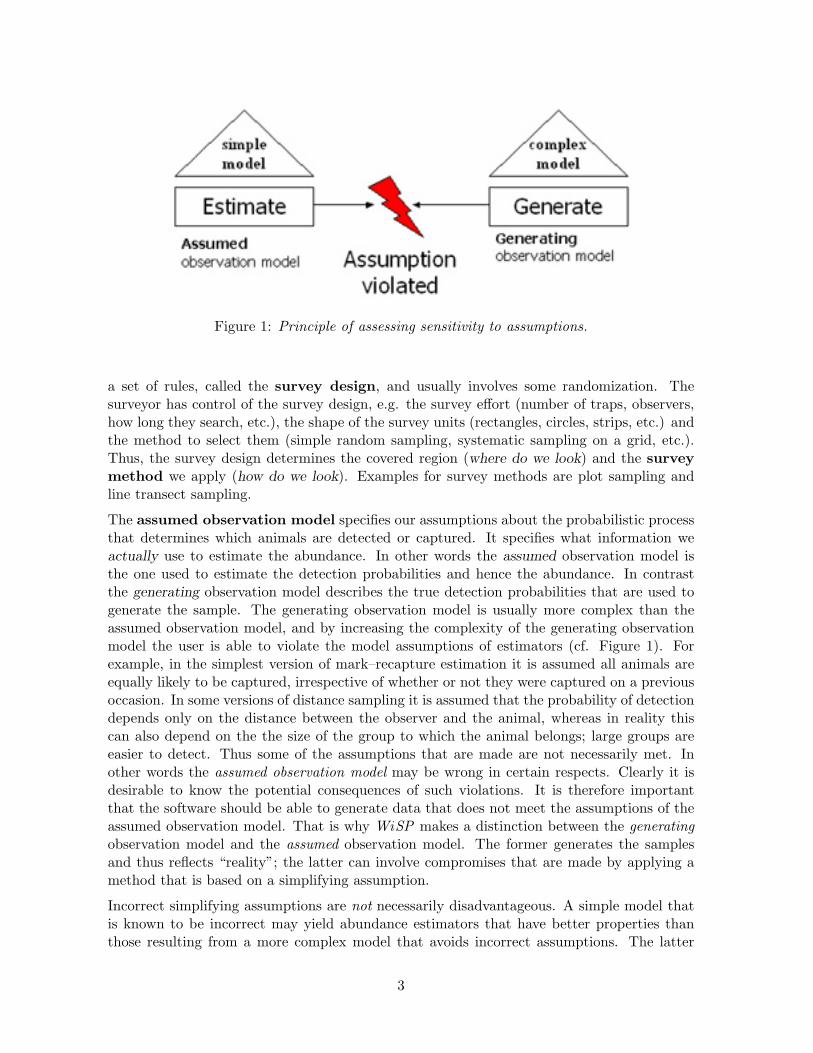
Figure 1: Principle of assessing sensitivity to assumptions.

a set of rules, called the survey design, and usually involves some randomization. Thesurveyor has control of the survey design, e.g. the survey effort (number of traps, observers,how long they search, etc.), the shape of the survey units (rectangles, circles, strips, etc.) andthe method to select them (simple random sampling, systematic sampling on a grid, etc.).Thus, the survey design determines the covered region (where do we look) and the surveymethod we apply (how do we look). Examples for survey methods are plot sampling andline transect sampling.

The assumed observation model specifies our assumptions about the probabilistic processthat determines which animals are detected or captured. It specifies what information weactually use to estimate the abundance. In other words the assumed observation model isthe one used to estimate the detection probabilities and hence the abundance. In contrastthe generating observation model describes the true detection probabilities that are used togenerate the sample. The generating observation model is usually more complex than theassumed observation model, and by increasing the complexity of the generating observationmodel the user is able to violate the model assumptions of estimators (cf. Figure 1). Forexample, in the simplest version of mark–recapture estimation it is assumed all animals areequally likely to be captured, irrespective of whether or not they were captured on a previousoccasion. In some versions of distance sampling it is assumed that the probability of detectiondepends only on the distance between the observer and the animal, whereas in reality thiscan also depend on the the size of the group to which the animal belongs; large groups areeasier to detect. Thus some of the assumptions that are made are not necessarily met. Inother words the assumed observation model may be wrong in certain respects. Clearly it isdesirable to know the potential consequences of such violations. It is therefore importantthat the software should be able to generate data that does not meet the assumptions of theassumed observation model. That is why WiSP makes a distinction between the generatingobservation model and the assumed observation model. The former generates the samplesand thus reflects “reality”; the latter can involve compromises that are made by applying amethod that is based on a simplifying assumption.

Incorrect simplifying assumptions are not necessarily disadvantageous. A simple model thatis known to be incorrect may yield abundance estimators that have better properties thanthose resulting from a more complex model that avoids incorrect assumptions. The latter

3

will generally lead to a smaller bias but to a larger standard error. That is because complexmodels have more parameters to be estimated and, for a given sample size, the precision withwhich the parameters can be estimated decreases with the number of parameters in the model.Furthermore, it is also possible to use a generating observation model that is simpler than theassumed observation model, for example to apply an estimation method that takes accountof animal–level heterogeneity when, in fact, there is none. This allows us to investigate theeffect of applying a method that is unnecessarily elaborate.

3 Abundance estimation in WiSP

This section will outline how the concepts introduced in Section 2 are implemented in WiSP ,that is the functions that are available to construct the state model, the survey design andthe generating observation model, the objects that are involved in these processes, and finally

Figure 2: The abundance estimation process in WiSP. Functions are shown as rectangles,objects as ellipses.

4

the functions used to compute point and interval estimates of abundance.

Figure 2 sketches the entire process in five steps starting with the specification of the statemodel and ending with the estimation of abundance. It also shows the WiSP core functions(rectangles) and core objects (ellipses) that are involved in each of the steps. Note thateach function named in Figure 2 (except for those involved in step I) actually representsa set of functions that carry out similar tasks. Thus “generate.sample” is implemented asgenerate.sample.pl in the context of plot sampling and as generate.sample.lt in linetransect sampling. The suffix at the end of the command (“.pl”,“.lt”, etc.) indicates whichsurvey method is to be applied.

The state model is specified by the functions generate.region, generate.density andsetpars.population. In the current implementation a region is simply a rectangle of givenheight and width and represents the total area on which the virtual population is located.The object density specifies the absolute (or relative) density of animals at all points in theregion. It can be represented as a surface over the survey region (Figure 3) and is used toassign positions to the animal groups in the region. (Strictly speaking the object “density”specifies the expected density; the actual positions are allocated at random.)

Figure 3: Example of a complex density with a linear trend, two strips of zero density (e.g.rivers) and a hotspot (a sub-region of unusually high density).

WiSP offers a set of functions that enable the user to conveniently generate and modify den-sities and thereby to investigate the properties of different survey methods and estimatorsunder a variety of assumptions regarding the spatial distribution of the animals in the survey

5

region. The specific characteristics of animal groups and of the individual animals are con-trolled by the function setpars.population. This determines the number of animal groupsin the population, the distribution of group sizes and the exposure distribution of each group(i.e. their detectability/catchability). The user may also associate additional characteristicswith each animal (e.g. age, gender, etc. ). This information is held in an object of the classpars.population. (Parameter objects are not displayed in Figure 2 for reasons of clarity.)The objects region, density and pars.population contain the information needed to gen-erate a population object. This is done by the function generate.population, as displayedin Figure 4.

Figure 4: Generating a realization of a population from its component objects.

The properties of the survey design that is to be used to survey the population are specifiedby a function of the type setpars.design. The currently implemented designs are plotsampling, mark-recapture methods, removal methods (including catch-effort and change-in-ratio), distance methods (line- and point-transects) and nearest-neighbour methods. Thus,for example in the case of line-transect sampling the function setpars.design.lt is used tospecify the number and width of the transects, how detectability of an animal is to dependon its distance from the trackline and on animal–level characteristics such as exposure, groupsize and gender. In the case of a mark-recapture survey the function setpars.design.cr isused to specify the probability that an animal will be captured on each occasion, and howthat probability is to depend on its characteristics including its capture history. For exampleanimals may become “trap-shy” or “trap-happy”. Setting up a specific survey design usuallyinvolves some randomization, a task carried out by a function of the type generate.design.

Having generated a virtual population and a specific survey design one is in a position to carryout the survey. The functions of the type generate.sample use the detection probabilitiesdelivered by the corresponding function of the type setpars.survey to generate a surveysample. Figure 5 shows an example plot of a sample object.

The generating observation model is defined by a function of the type setpars.survey.

6

Figure 5: Example of a point transect sample.

It uses a detection function that computes the detection probabilities for all animals in thepopulation. Therefore it needs the design- and the population object, as well as optionaluser–defined input parameters that specify additional details relating to the probability ofdetection. The generating observation model and the survey design are related because,among other things, the latter determines where we look and how hard we look, but there isalso an important distinction between them. The former determines the detection/captureprobabilities that can depend on properties of the population (e.g. the exposure distribution)that are not taken into account by the survey design. For example the detection can be madeto depend on the age of an animal whereas this is not taken into account in the survey design,e.g. the age is not recorded in the survey. It is precisely this distinction that enables us toassess the performance of estimators when the assumptions of the assumed observation modelare violated.

The sample, that is the particular subset of the population that is detected or captured,depends on chance in up to three distinct ways. There is the random variation in the statemodel, for example the positions and exposures of the animals in a population. Secondly thesurvey design can involve randomization, for example in the positioning of the transects in linetransect sampling. Finally, for a given population and a given design, chance is involved indetermining which particular animals are detected or captured. By means of simulation it ispossible to investigate the effect of these sources of variation either collectively or separately.For example, by repeatedly surveying a fixed population using a fixed line transect design onecan assess the effect of the remaining source of variation on the behavior of the abundanceestimator.

A sample object in WiSP contains the information that is available to the researcher oncompletion of a real survey. In plot sampling one has the counts in each plot; in line transectone has the distances of each detected group to the centerline and, possibly, other informationabout animal-level variables such as group sizes. Sample objects also contain details aboutthe particular survey method that was used, for example, the number and size of the samplingunits (plots, transects) and other survey-related variables such as sampling effort.

7

In the last step of the process, the sample object is passed to estimation functions whichcompute point and interval estimates of abundance. Different types of surveys generate verydifferent types of sample information and therefore require different estimators. Thus eachtype of survey requires a corresponding set of estimation functions. The current implementa-tion of WiSP computes maximum likelihood estimation for all survey methods covered as wellas a number of traditional alternatives. At least one method for interval estimation is imple-mented for each design. Parametric bootstrap confidence intervals are available for all casesbut alternative methods (non-parametric bootstrap, asymptotic methods, profile likelihood)are also available for some designs.

4 Survey methods

We give a brief outline of the survey methods that are currently implemented in WiSP .Details are given in Borchers et al (2002).

Plot sampling covers methods such as quadrat sampling and strip sampling. Althoughthese may differ in their implementation they are effectively identical from a statistical pointof view; they differ only in the shape of the survey units. It is assumed that all animals inthe covered region are detected with certainty.

Removal, catch–effort and change–in–ratio methods require at least two survey oc-casions and involve no assumptions regarding the state model. The design is “search every-where”. The animals captured on each occasion are counted and removed from the population.The estimation model of the simple removal method assumes that capture probabilities areequal for all animals, that they remain the same on every survey occasion, and that thecaptures are independent. These assumptions are relaxed in catch–effort estimation modelsin which the capture probability is allowed to depend on the catch–effort on each occasion.The estimates are based on changes in the catch–per–unit–effort rather on changes in thecatch. The estimation model of the change–in–ratio method constitutes a different kind ofrefinement. It makes use of changes in the proportions of animals of various types (sex, age,etc.) following removals of known numbers of animals of each type, but avoids the need totake account of the catch–effort on each survey occasion.

Mark–recapture methods are similar to removal methods but the captured animals arenot removed; they are marked and replaced in the population. The methods vary in com-plexity depending on the model assumptions. In the simplest case one assumes that on eachoccasion each animal is equally likely to be captured. Other models allow for various kindsof heterogeneity, for example that the capture probabilities depend on certain (observable)features of the captured animals, on their capture history and so on.

Distance sampling methods estimate the relationship between the detection probabilityand the distance of detected animals to the centerline of a strip of given width (line transectsampling) or to the center of a circle of given radius (point transect sampling). It is assumedthat detection is certain if the distance is zero. This assumption is unrealistic for someanimals (e.g. whales) and can be relaxed by using double platform methods which arecurrently not implemented in WiSP . Only a single survey is required in distance sampling;randomization is usually applied to select the strips (or circles) that make up the coveredregion. Here too the methods vary in complexity depending on the assumptions made and

8

the type of information collected.

In nearest neighbor sampling objects (animals or plants) in the survey region are randomlysampled, and the distances to their nearest neighbors are recorded. In point–to–nearest–object sampling, points within the survey regions are selected at random and the distancefrom each point to the nearest object is measured. If we assume that objects are independentlyand uniformly distributed throughout the survey region then the distribution of nearest-objectdistances is the same under both approaches. The estimator of abundance is based on thefact there is an inverse relationship between the average distance to the nearest object andthe density of objects in the region.

5 Sensitivity analyses

In this section we illustrate how WiSP can be applied to assess the sensitivity of two abun-dance estimation methods to model assumptions. We also compare two strategies for plotsampling. Details of the survey designs and the estimators are given in, e.g., Borchers et al.(2002).

5.1 Simple mark-recapture model

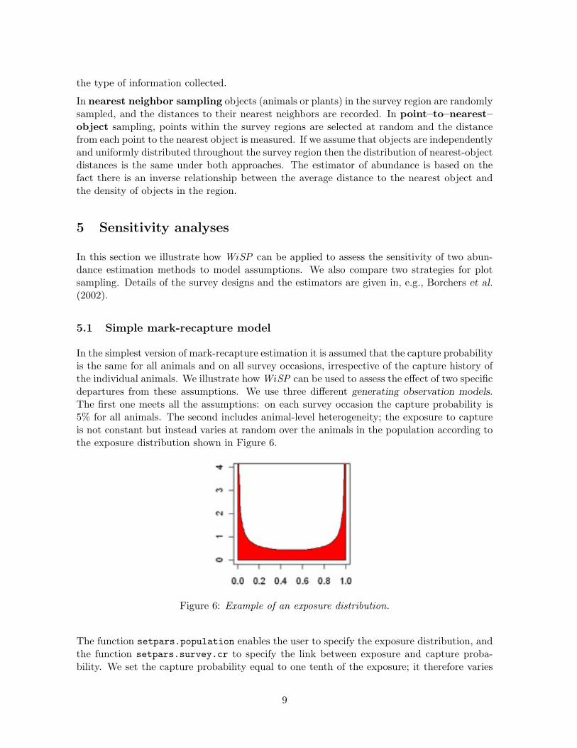
In the simplest version of mark-recapture estimation it is assumed that the capture probabilityis the same for all animals and on all survey occasions, irrespective of the capture history ofthe individual animals. We illustrate how WiSP can be used to assess the effect of two specificdepartures from these assumptions. We use three different generating observation models.The first one meets all the assumptions: on each survey occasion the capture probability is5% for all animals. The second includes animal-level heterogeneity; the exposure to captureis not constant but instead varies at random over the animals in the population according tothe exposure distribution shown in Figure 6.

Figure 6: Example of an exposure distribution.

The function setpars.population enables the user to specify the exposure distribution, andthe function setpars.survey.cr to specify the link between exposure and capture proba-bility. We set the capture probability equal to one tenth of the exposure; it therefore varies

9

between 0 and 10%. The particular U-shaped exposure distribution displayed in Figure 6 hasdistinct modes at 0 and 1. Thus many animals in this virtual population are very unlikely tobe captured, and many are captured with probability close to 10%.

The third generating observation model incorporates “trap-shyness”. Here we set the proba-bility capturing an animal for the first time to 5% and reduced this to 3% for animals thathad been captured on a previous occasion.

We generated 10000 populations of size 500 and surveyed each population using each ofthe three generating observation models described above. A three-occasion survey was usedthroughout. Estimation was carried out using the same assumed observation model, i.e.assuming that the capture probability is constant for all animals and on all three surveyoccasions. Essentially the estimator is based on the ratio of unmarked to marked animalscaptured on the second and third survey occasions. The results are show in Figure 7.

Figure 7: Boxplots of estimates based a simple mark-recapture model estimator for threedifferent generating observation models.

Figure 7 shows that even in the ideal circumstance in which all assumptions are met themaximum likelihood estimator tends to overestimate abundance. But this bias is modestcompared to that in the other two cases considered.

The gross underestimates in the heterogeneous case can be explained by the fact that asubstantial proportion of animals have very low exposure (Figure 6.) Such animals are veryseldom captured and are thus “invisible” to this type of survey. In effect they are not countedas members of the population.

10

Trap-shyness leads to the situation in which the subpopulation of marked animals become“under-represented” in subsequent samples, whereas the estimator is based on the assumptionthat the marked and unmarked subpopulations will be represented proportionately. This leadsto overestimates of the number of unmarked animals and hence to overestimates of the totalabundance.

5.2 Change-in-ratio method

The simplest change-in-ratio estimator relies on the assumption that the detection probabilitydoes not depend on animal-level variables, such as sex, age and so on. We assess the behaviorof this estimator in the case where this assumption is met and in one case where it is violated.

We generated 10000 virtual populations each comprising 500 animals. The sex of each animalwas determined at random with probability 0.5 of being male/female. The survey designinvolved two survey occasions. In the first experiment we used a capture probability of 50%for both males and females, i.e. the generating and the assumed observation models were thesame. In the second experiment the capture probability was set to 60% for males and 40%for females. Boxplots of the resulting estimates are displayed in Figure 8.

Figure 8: Boxplots of abundance estimates using the catch-in ratio method for a populationcomprising 500 animals.

11

Figure 9: Plot of a regular grid design (left) and a random grid design (right), They have thesame number of plots and cover the same area.

In the case where the model assumptions are met the distribution of the estimator is slightlyskewed but the estimator is approximately unbiased. However, when the detection probabilitydiffers for males and females, i.e. when there is animal-level heterogeneity, the estimatorunderestimates abundance . There also is the marked increase in the variance of the estimator.Evidently the less rapid removal of males from the population does not compensated for themore rapid removal of females. Clearly the behavior of the estimator is not robust to violationsto the assumption of homogeneity.

5.3 Plot design: random vs. regular plots

In our last example we assess the performance of two plot survey designs. The issue hereis not to investigate the effect of violating model assumptions, but rather to compare theperformance of two different survey designs over a range of circumstances. Plot sample esti-mation is very easy: From the region under consideration (of area A) one selects a subregion(of area a) and counts all the animals in the subregion. The estimator of abundance for theentire region is simply the number of animals counted in the subregion multiplied by A

a . Inpractice the subregion usually comprises a number of plots of equal size. Generally the plotsare placed at random over the region, or they are placed systematically on the vertices of arectangular grid covering the region (Figure 9).

Figure 10: Three spatial densities (a) constant (b) linear (c) complex.

Here we compare the performance of the abundance estimator for these two strategies forplacing the plots. In particular we compare them under three different assumptions about

12

the spatial distribution of the animals.

We generated 10000 replications of 3 virtual populations of size 500. The populations differin their spatial distributions, i.e. the density of animals over the region. (See Figure 10.)In the first case the density is constant over the region; in the second it increases linearlyin the direction NW to SE, and in the third case it is a more complex entity that includesa “hotspot” in the south-east corner and a river (with no animals) running approximatelynorth-south.

Every population was surveyed using each of the two plot designs. The first design placed theplots on a regular grid and the second placed the plots at random. Typical plot placementsare show in Figure 9.

Figure 11: Abundance estimates based on regular and random grid designs for the three den-sities shown in Figure 9. The population size is 500.

A boxplot of the resulting abundance estimates are shown in Figure 11. These results indicatethat there is little difference in the distribution of the estimates when the population densitywas constant or linear. Noticeable differences arise in the case where the density was complex.The estimators are approximately unbiased, although the regular case exhibited a tendencyto overestimate slightly (3%). Theoretically the random case leads to an unbiased estimatorwhereas the regular case can be biased because regular plots can systematically “miss” localfeatures of the underlying density. However, the most prominent feature in Figure 11 is thesubstantially larger variance of the estimator based on random plots when the density iscomplex. In retrospect the reason for this is obvious. The randomly placed plots sometimesall ”miss” the hotspot on the SE corner of the region thus leading to an underestimate ofabundance, and sometimes “too many” plots land on, or near, the hotspot thus leading to anoverestimate of abundance. In contrast the regular plots are always in fixed positions and so

13

the estimator is not subject to the above source of random variation. Thus although regulardesigns are not guaranteed to lead to unbiased estimators, the variance of the latter can besubstantially smaller than that resulting from randomly placed plots, especially when thespatial distribution of animals is complex. In experimental design randomization is generallyregarded as a “good thing”, mainly because it avoids bias. Our experiment suggests that thebias that results by using a regular design can be insubstantial compared to the increasedstandard error that results by using a random design.

6 Concluding remarks

WiSP is primarily intended as a teaching tool to illustrate the basic principles underlyingthe most popular (closed population) abundance estimation techniques and to study theirstrengths and weaknesses. In its current form WiSP does not have the functionality of themore comprehensive software packages available for the analysis of field data. (Useful lists oflinks can be found at www.phidot.org/software and www.mbr.nbs.gov/software.html .)

The free availability of R was an important consideration in selecting it as the language forWiSP but the other advantages that R offers were even more important in terms of futuredevelopment of the WiSP library. The code can be made available in text form, which makesit conveniently accessible to users who wish to modify it, to define new functions to cover agreater range of survey designs, or to introduce additional features in the state process. Theobject–orientated design of WiSP that is facilitated by R renders the task of making suchmodifications and enhancements incomparably less forbidding than would be the case if alanguage without this feature had been used.

7 References

Borchers, D.L. Buckland, S.T. & Zucchini W. (2002). Estimating Animal Abundance: ClosedPopulations. Springer-Verlag, London.

Hornik (2002),“The R FAQ”, http://www.gnu.org/copyleft/gpl.html

Ihaka, Ross and Gentleman, Robert (1996), R: A Language for Data Analysis and Graphics,Journal of Computational and Graphical Statistics, 5(3), 299-314.

Seber, G.A.F. (1982), The Estimation of Animal Abundance and Related Information Pa-rameters. 2nd edition, Griffin, London.

14