a weighted nearest neighbor algorithm for learning with ...1022664626993.pdf · a weighted nearest...

Machine Learning, 10, 57-78 (1993)© 1993 Kluwer Academic Publishers, Boston. Manufactured in The Netherlands.

A Weighted Nearest Neighbor Algorithm forLearning with Symbolic Features

SCOTT COST [email protected] SALZBERG [email protected] of Computer Science, Johns Hopkins University, Baltimore, MD 21218

Editor: Richard Simon

Abstract. In the past, nearest neighbor algorithms for learning from examples have worked best in domains inwhich all features had numeric values. In such domains, the examples can be treated as points and distance metricscan use standard definitions. In symbolic domains, a more sophisticated treatment of the feature space is required.We introduce a nearest neighbor algorithm for learning in domains with symbolic features. Our algorithm calculatesdistance tables that allow it to produce real-valued distances between instances, and attaches weights to the instancesto further modify the structure of feature space. We show that this technique produces excellent classificationaccuracy on three problems that have been studied by machine learning researchers: predicting protein secondarystructure, identifying DNA promoter sequences, and pronouncing English text. Direct experimental comparisonswith the other learning algorithms show that our nearest neighbor algorithm is comparable or superior in allthree domains. In addition, our algorithm has advantages in training speed, simplicity, and perspicuity. We con-clude that experimental evidence favors the use and continued development of nearest neighbor algorithms fordomains such as the ones studied here.

Keywords. Nearest neighbor, exemplar-based learning, protein structure, text pronunciation, instance-based learning

1. Introduction

Learning to classify objects is a fundamental problem in artificial intelligence and otherfields, one which has been attacked from many angles. Despite many successes, there aresome domains in which the task has proven very difficult, due either to the inherent diffi-culty of the domain or to the lack of sufficient data for learning. For example, instance-based learning programs (also called exemplar-based (Salzberg, 1990) or nearest neighbor(Cover & Hart, 1967) methods), which learn by storing examples as points in a featurespace, require some means of measuring distance between examples (Aha, 1989; Aha &Kibler, 1989; Salzberg, 1989; Cost & Salzberg, 1990). An example is usually a vector offeature values plus a category label. When the features are numeric, normalized Euclideandistance can be used to compare examples. However, when the feature values have sym-bolic, unordered values (e.g., the letters of the alphabet, which have no natural inter-letter"distance"), nearest neighbor methods typically resort to much simpler metrics, such ascounting the features that match. (Towell et al. (1990) recently used this metric for thenearest neighbor algorithm in their comparative study.) Simpler metrics may fail to capturethe complexity of the problem domains, and as a result may not perform well.

In this paper, we present a more sophisticated instance-based algorithm designed fordomains in which some or all of the feature values are symbolic. Our algorithm constructs

58 S. COST AND S. SALZBERG

modified "value difference" tables (in the style of Stanfill & Waltz (1986)) to produce anon-Euclidean distance metric, and we introduce the idea of "exception spaces" that resultwhen weights are attached to individual examples. The combination of these two techniquesresults in a robust instance-based learning algorithm that works for any domain with sym-bolic feature values. We describe a series of experiments demonstrating that our algorithm,PEBLS, performs well on three important practical classification problems. Comparisonsgiven below show that our algorithm's accuracy is comparable to back propagation, deci-sion trees, and other learning algorithms. These results support the claim that nearest neigh-bor algorithms are powerful classifiers even when all features are symbolic.

1.1. Instance-based learning versus other models

The power of instance-based methods has been demonstrated in a number of importantreal world domains, such as prediction of cancer recurrence, diagnosis of heart disease,and classification of congressional voting records (Aha & Kibler, 1989; Salzberg, 1989).Our experiments demonstrate that instance-based learning (IBL) can be applied effectivelyin three other domains, all of which have features with unordered symbolic values: (1) predic-tion of protein secondary structure, (2) word pronunciation, and (3) prediction of DNApromoter sequences. These domains have received considerable attention from connectionistresearchers who employed the back propagation learning algorithm (Sejnowski & Rosenberg,1986; Qian & Sejnowski, 1988; Towell et al., 1990). In addition, the word pronunciationproblem has been the subject of a number of comparisons using other machine learningalgorithms (Stanfill & Waltz, 1986; Shavlik et al., 1989; Dietterich et al., 1990). All ofthese domains represent problems of considerable practical importance, and all have sym-bolic feature values, which makes them difficult for conventional nearest neighbor algo-rithms. We will show how our nearest neighbor algorithm, PEBLS, which is based on Stanfilland Waltz's (1986) "value difference" method, can produce highly accurate predictive modelsin each of these domains.

Our intent is to compare IBL to other learning methods in three respects: classificationaccuracy, speed of training, and perspicuity (i.e., the ease with which the algorithm andits representation can be understood). Because of its comparable performance in the firstrespect, and its superiority in the latter two, we argue that IBL is often preferable to otherlearning algorithms for the types of problem domains considered in this paper. Instance-based learning has been shown to compare favorably to other algorithms (e.g., decisiontrees and rules) on a wide range of domains in which feature values were either numericor binary (e.g., Aha, 1989; Aha & Kibler, 1989; Aha et al., 1991; Salzberg, 1989). Thispaper presents similar evidence in terms of classification accuracy for domains with sym-bolic feature values. However, before describing these domains, we should consider otheradvantages that instance-based learning algorithms can provide.

Training time. Most neural net learning algorithms require vastly more time for trainingthan other machine learning methods. Training is normally performed by repeatedly present-ing the network with instances from a training set, and allowing it gradually to convergeon the best set of weights for the task, using (for example) the back propagation algorithm.

LEARNING WITH SYMBOLIC FEATURES 59

Weiss and Kapouleas (1989), Mooney et al. (1989), and Shavlik et al. (1989) report thatback propagation's training time is many orders of magnitude greater than training timefor algorithms such as ID3, frequently by factors of 100 or more. In addition, neural netalgorithms have a number of parameters (e.g., the "momentum" parameter) that need tobe tweaked by the programmer, and may require much additional time. The Weiss andKapouleas experiments required many months of the experimenters' time to produce resultsfor back propagation, while the other algorithms typically required only a few hours. Theonly parameter that might be adjusted for our algorithm is the value of r in our distancemetric (see below), and we only consider two possible values, r = 1 and r = 2.

Our nearest neighbor algorithm requires very little training time, both in terms of experi-menter's time and processing time. Below we present two versions of the PEBLS algorithm,one slightly more complex than the other. The simpler version, which is called the"unweighted" version in our experimental section below, requires O(dn + dv2) time fortraining, where n is the number of examples, d is the number of features (dimensions)per example, and v is the number of values that a feature may have. (In general n is muchlarger than v2; hence the complexity is usually O(dn).) The more complex version ofPEBLS incrementally computes weights for exemplars, and requires O(dn2) time for ntraining instances.1 After training, classification time for a nearest neighbor system is atworst O(dn), which is admittedly slow compared to other algorithms.

Nearest neighbor methods lend themselves well to parallelization, which can producesignificantly faster classification times. Each example can be assigned to a separate proc-essor in a parallel architecture, or, if there are not enough processors, the examples canbe divided among them. When the number of processors is as large as the training set,classification time may be reduced to O(d log n). We implemented our system on a setof four loosely-coupled transputers as well as on a conventional architecture, and otherrecent efforts such as FGP (Fertig & Gelernter, 1991) use larger numbers of parallel proc-essors. The MBRtalk system of Waltz and Stanfill (1986) implemented a form of k-nearest-neighbor learning using a tightly-coupled massively parallel architecture, the 64,000-processor Connection Machine™.

Perspicuity. Our instance-based learning algorithm is also more transparent in its operationthan other learning methods. The algorithm itself is nothing if not straightforward: definea measure of distance between values, compare each new instance to all instances in memory,and classify according to the category of the closest. Decision tree algorithms are perhapsequally straightforward at classification time—just pass an example down through the treeto get a decision. Neural net algorithms are fast at classification time, but are not as trans-parent—weights must be propagated through the net, summed, and passed through a filter(e.g., a threshold) at each layer. The only complicated part of our method is the computa-tion of our distance tables, which are computed via a fixed statistical technique based onfrequency of occurrence of values. However, this is certainly no more complicated than theentropy calculations of decision tree methods (e.g., Quinlan (1986)) or the weight adjust-ment routines used in back propagation. The tables themselves provide some insight intothe relative importance of different features—we noticed, for instance, that several of thetables for the protein folding data were almost identical (indicating that the features werevery similar). The instance memory of an IBL system is readily accessible, and can be


examined in numerous ways. For example, if a human wants to know why a particular clas-sification was made, the system can simply present the instance from its memory that wasused for classification. Human experts commonly use such explanations; for example, whenasked to justify a prediction about the economy, experts typically produce another, similareconomic situation from the past. Neural nets do not yet provide any insight into why theymade the classification they did, although some recent efforts have explored new methodsfor understanding the content of a trained network (Hanson & Burr, 1990). It is also relativelyeasy to modify our algorithm to include domain specific knowledge: if the relative impor-tance of the features is known, the features may be weighted accordingly in the distanceformula (Salzberg, 1989).

Taken together, the advantages listed above make it clear that IBL algorithms have a numberof benefits with respect to competing models. However, in order to be considered a realisticpractical learning technique, IBL must still demonstrate good classification accuracy. Whenthe problem domain has symbolic features, the obvious distance metric for IBL, countingthe number of features that differ, does not work well. (This metric is called the "overlap"metric.) Our experimental results show that a modified value-difference metric can proc-ess symbolic values exceptionally well. These results, taken together with other results ondomains with numeric features (e.g., Aha, 1990; Aha et al., 1991), show that IBL algo-rithms perform quite well on a wide range of problems.

2. Learning algorithms

Back propagation is the most widely used and understood neural net learning algorithm,and will be used as the basis of comparison for the experiments in this paper. Althoughearlier approaches, most notably the perceptron learning model, were unable to classifygroups of concepts that are not linearly separable, back propagation can overcome thisproblem. Back propagation is a gradient descent method that propagates error signals backthrough a multi-layer network. It has been described in many places (e.g., Rumelhart etal., 1986; Rumelhart & McClelland, 1986), and readers interested in a more detailed descrip-tion should look there. We will use the decision tree algorithm ID3 (Quinlan, 1986) asthe basis for comparison with decision tree algorithms. In addition, we have comparedthe performance of our algorithm to other methods used on the same data for each of thedomains described in section 3. Where appropriate, we present results from domain-specificclassification methods.

2.1. Instance-based learning

Our instance-based learning algorithm, like all such algorithms, stores a series of traininginstances in its memory, and uses a distance metric to compare new instances to those stored.New instances are classified according to the closest exemplar from memory. Our algorithmis implemented in a program called PEBLS, which stands for Parallel Exemplar-BasedLearning System.2 For clarity, we use the term "example" to mean a training or test exam-ple being shown to the system for the first time. We use the term "exemplar" (following


the usage of Salzberg (1991)) to refer specifically to an instance that has been previouslystored in computer memory. Such exemplars may have additional information attached tothem (e.g., weights). The term "instance" covers both examples and exemplars.

PEBLS was designed to process instances that have symbolic feature values. The heartof the PEBLS algorithm is the way in which it measures distance between two examples.This consists of essentially three components. The first is a modification of Stanfill andWaltz's (1986) Value Difference Metric (VDM), which defines the distance between differ-ent values of a given feature. We call our method MVDM, for Modified Value DifferenceMetric. Our second component is a standard distance metric for measuring the distancebetween two examples in a multi-dimensional feature space. Finally, the distance is modifiedby a weighting scheme that weights instances in memory according to their performancehistory (Salzberg, 1989; 1990). These components of the distance calculation are describedin sections 2.2 and 2.3.

PEBLS requires two passes through the training set. During the first pass, feature valuedifference tables are constructed from the instances in the training set, according to theequations for the Stanfill Waltz VDM. In the second pass, the system attempts to classifyeach instance by computing the distance between the new instance and previously storedones. The new instance is then assigned the classification of the nearest stored instance.The system then checks to see if the classification is correct, and uses this feedback toadjust a weight on the old instance (this weight is described in detail in section 2.3). Finally,the new instance is stored in memory. During testing, examples are classified in the samemanner, but no modifications are made to memory or to the distance tables.

2.2. The Stanfill-Waltz VDM

In 1986, Stanfill and Waltz presented a powerful new method for measuring the distancebetween values of features in domains with symbolic feature values. They applied theirtechnique to the English pronunciation problem with impressive initial results (Stanfill &Waltz, 1986). Their Value Difference Metric (VDM) takes into account the overall similarityof classification of all instances for each possible value of each feature. Using this method,a matrix defining the distance between all values of a feature is derived statistically, basedon the examples in the training set. The distance 5 between two values (e.g., two aminoacids) for a specific feature is defined in Equation 1:

In the equation, V1 and V2 are two possible values for the feature, e.g., for the proteindata these would be two amino acids. The distance between the values is a sum over alln classes. For example, the protein folding experiments in section 4.1 had three categories,so n = 3 for that data. C1i is the number of times V1 was classified into category i, C1

is the total number of times value 1 occurred, and k is a constant, usually set to 1.


Using Equation 1, we compute a matrix of value differences for each feature in the inputdata. It is interesting to note that the value difference matrices computed in the experimentsbelow are quite similar overall for different features, although they differ significantly forsome value pairs.

The idea behind this metric is that we wish to establish that values are similar if theyoccur with the same relative frequency for all classifications. The term C1i/C1 representsthe likelihood that the central residue will be classified as i given that the feature in ques-tion has value Vl. Thus we say that two values are similar if they give similar likelihoodsfor all possible classifications. Equation 1 computes overall similarity between two valuesby finding the sum of the differences of these likelihoods over all classifications.

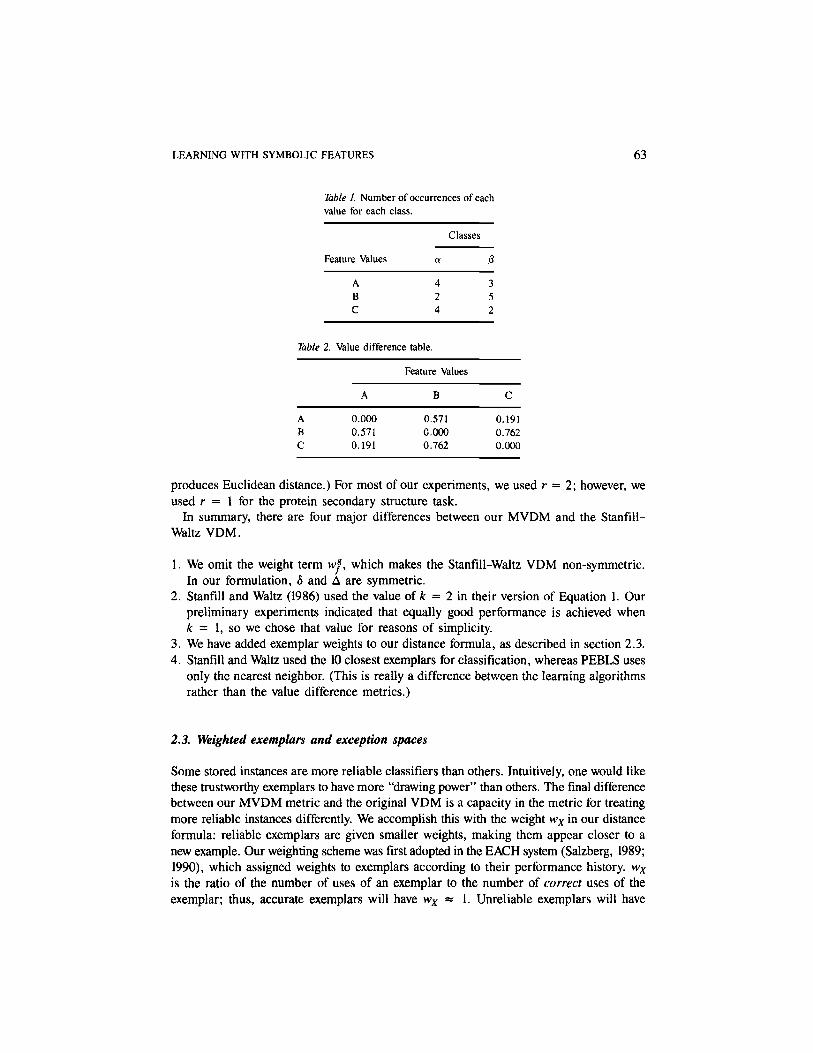
Consider the following example. Say we have a pool of instances for which we examinea single feature that takes one of three values, A, B, and C. Two classifications, a and3, are possible. From the data we construct Table 1, in which the table entries representthe number of times an instance had a given feature value and classification. From thisinformation we construct a table of distances as follows. The frequency of occurrence ofA for class a is 57.1%, since there were 4 instances classified as a out of 7 instances withvalue A. Similarly, the frequencies of occurrence for B and C are 28.6% and 66.7%, respec-tively. The frequency of occurrence of A for class 3 is 42.9 %, and so on. To find the distancebetween A and B, we use Equation 1, which yields |4/7 - 2/71 + |3/7 - 5/71 = 0.571.The complete table of distances is shown in Table 2. Note that we construct a differentvalue difference table for each feature; if there are 10 features, we will construct 10 tables.

Equation 1 defines a geometric distance on a fixed, finite set of values—that is, the prop-erty that a value has distance zero to itself, that it has a positive distance to all other values,that distances are symmetric, and that distances obey the triangle inequality. We can sum-marize these properties as follows:

Stanfill and Waltz's original VDM also used a weight term wf, which makes their versionof 6 non-symmetric; e.g., 8(a, b) ^ 5(b, a). A major difference between their metric (VDM)and ours (MVDM) is that we omit this term, which makes 5 symmetric.

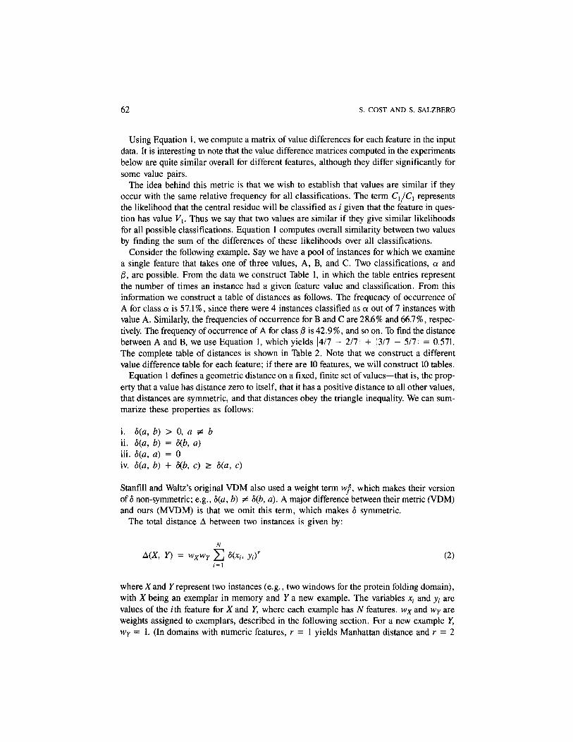
The total distance A between two instances is given by:

where X and Y represent two instances (e.g., two windows for the protein folding domain),with X being an exemplar in memory and Y a new example. The variables xi and yi arevalues of the ith feature for X and Y, where each example has N features. wx and WY areweights assigned to exemplars, described in the following section. For a new example Y,wY = 1. (In domains with numeric features, r = 1 yields Manhattan distance and r = 2


Table 1. Number of occurrences of eachvalue for each class.

Feature Values

ABC

Classes

a

424

&

352

Table 2. Value difference table.

ABC

Feature Values

A

0.0000.5710.191

B

0.5710.0000.762

C

0.1910.7620.000

produces Euclidean distance.) For most of our experiments, we used r = 2; however, weused r = 1 for the protein secondary structure task.

In summary, there are four major differences between our MVDM and the Stanfill-Waltz VDM.

1. We omit the weight term wf, which makes the Stanfill-Waltz VDM non-symmetric.In our formulation, 8 and A are symmetric.

2. Stanfill and Waltz (1986) used the value of k = 2 in their version of Equation 1. Ourpreliminary experiments indicated that equally good performance is achieved whenk = 1, so we chose that value for reasons of simplicity.

3. We have added exemplar weights to our distance formula, as described in section 2.3.4. Stanfill and Waltz used the 10 closest exemplars for classification, whereas PEBLS uses

only the nearest neighbor. (This is really a difference between the learning algorithmsrather than the value difference metrics.)

2.3. Weighted exemplars and exception spaces

Some stored instances are more reliable classifiers than others. Intuitively, one would likethese trustworthy exemplars to have more "drawing power" than others. The final differencebetween our MVDM metric and the original VDM is a capacity in the metric for treatingmore reliable instances differently. We accomplish this with the weight wx in our distanceformula: reliable exemplars are given smaller weights, making them appear closer to anew example. Our weighting scheme was first adopted in the EACH system (Salzberg, 1989;1990), which assigned weights to exemplars according to their performance history. wx

is the ratio of the number of uses of an exemplar to the number of correct uses of theexemplar; thus, accurate exemplars will have wx = 1. Unreliable exemplars will have


wx > 1, making them appear further away from a new example. These unreliable exem-plars may represent either noise or "exceptions"—small areas of feature space in whichthe normal rule does not apply. The more times an exemplar is incorrectly used for classifica-tion, the larger its weight grows. An alternative scheme for handling noisy or exceptionalinstances in the IBL framework is discussed by Aha and Kibler (1989), and elaborated fur-ther in Aha (1990). In their scheme, an instance is not used in the nearest-neighbor com-putation until it has proven itself to be an "acceptable" classifier. Acceptable instances arethose whose classification accuracies exceed the baseline frequency for a class by a fixedamount. (For example, if the baseline frequency of a class is 30%, an instance that wascorrect 80% of the time would be acceptable, whereas if the baseline frequency was 90%,the same instance would not be acceptable.) We should note that our technique is not designedprimarily to filter out noisy instances, but rather to identify exceptional instances. The dif-ference is that noisy instances should probably be ignored or discarded, whereas excep-tional instances should be retained, but used relatively infrequently.

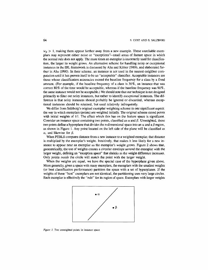
We differ from Salzberg's original exemplar weighting scheme in one significant aspect:the way in which exemplars (points) are weighted initially. The original scheme stored pointswith initial weights of 1/1. The effect which this has on the feature space is significant.Consider an instance space containing two points, classified as a and 3. Unweighted, thesetwo points define a hyperplane that divides the n-dimensional space into an a and a P region,as shown in Figure 1. Any point located on the left side of the plane will be classified as«, and likewise for $.

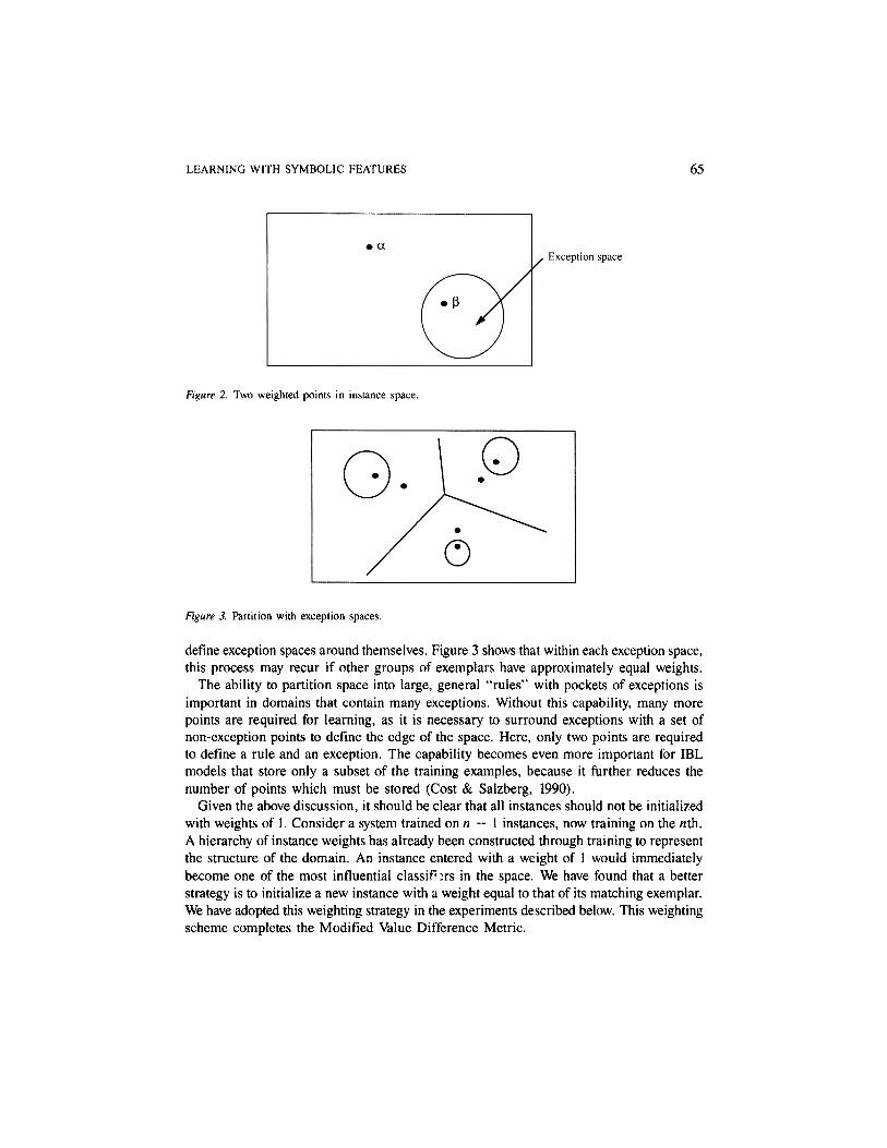
When PEBLS computes distance from a new instance to a weighted exemplar, that distanceis multiplied by the exemplar's weight. Intuitively, that makes it less likely for a new in-stance to appear near an exemplar as the exemplar's weight grows. Figure 2 shows that,geometrically, the use of weights creates a circular envelope around the exemplar with thelarger weight, defining an "exception space" that shrinks as the weight difference increases.Only points inside the circle will match the point with the larger weight.

When the weights are equal, we have the special case of the hyperplane given above.More generally, given a space with many exemplars, the exemplars with the smallest weights(or best classification performance) partition the space with a set of hyperplanes. If theweights of these "best" exemplars are not identical, the partitioning uses very large circles.Each exemplar is effectively the "rule" for its region of space. Exemplars with larger weights

Figure 1. Two unweighted points in instance space.


Figure 2. Two weighted points in instance space.

Figure 3. Partition with exception spaces.

define exception spaces around themselves. Figure 3 shows that within each exception space,this process may recur if other groups of exemplars have approximately equal weights.

The ability to partition space into large, general "rules" with pockets of exceptions isimportant in domains that contain many exceptions. Without this capability, many morepoints are required for learning, as it is necessary to surround exceptions with a set ofnon-exception points to define the edge of the space. Here, only two points are requiredto define a rule and an exception. The capability becomes even more important for IBLmodels that store only a subset of the training examples, because it further reduces thenumber of points which must be stored (Cost & Salzberg, 1990).

Given the above discussion, it should be clear that all instances should not be initializedwith weights of 1. Consider a system trained on n - 1 instances, now training on the nth.A hierarchy of instance weights has already been constructed through training to representthe structure of the domain. An instance entered with a weight of 1 would immediatelybecome one of the most influential classifiers in the space. We have found that a betterstrategy is to initialize a new instance with a weight equal to that of its matching exemplar.We have adopted this weighting strategy in the experiments described below. This weightingscheme completes the Modified Value Difference Metric.


3. Domains

We chose for our comparisons three domains that have received considerable attention fromthe machine learning research community: the word-pronunciation task (Sejnowski &Rosenberg, 1986; Shavlik et al., 1989), the prediction of protein secondary structure (Qian& Sejnowski, 1988; Holley & Karplus, 1989), and the prediction of DNA promoter se-quences (Towell et al., 1989). Each domain has only symbolic-valued features; thus, ourMVDM is applicable whereas standard Euclidean distance is not. Sections 3.1-3.3 describethe three databases and the problems they present for learning.

3.1. Protein secondary structure

Accurate techniques for predicting the folded structure of proteins do not yet exist, despiteincreasingly numerous attempts to solve this problem. Most techniques depend in part onprediction of the secondary structure from the primary sequence of amino acids. The secon-dary structure and other information can then be used to construct the final, tertiary struc-ture. Tertiary structure is very difficult to derive directly, requiring expensive methods ofX-ray crystallography. The primary sequence, or sequence of amino acids which constitutea protein, is relatively easy to discover. Attempts to predict secondary structure involvethe classification of residues into three categories: a helix, 0 sheet, and coil. Three of themost widely used approaches to this problem are those of Robson (Gamier et al., 1978),Chou and Fasman (1978), and Lim (1974), which produce classification accuracies rangingfrom 48% to 58%. Other, more accurate techniques have been developed for predictingtertiary from secondary structure (e.g., Cohen et al., 1986; Lathrop et al., 1987), but theaccurate prediction of secondary structure has proven to be an extremely difficult task.

The learning problem can be described as follows. A protein consists of a sequence ofamino acids bonded together as a chain. This sequence is known as the primary structure.Each amino acid in the chain can be one of twenty different acids. At the point at whichtwo acids join in the chain, various factors including their own chemical properties deter-mine the angle of the molecular bond between them. This angle, for our purposes, is char-acterized as one of three different types of "fold": a helix, 3 sheet, or coil. In other words,if a certain number of consecutive acids (hereafter residues) in the chain join in a mannerwhich we call a, that segment of the chain is an a helix. This characterization of foldtypes for a protein is known as the secondary structure. The learning problem, then, is:given a sequence of residues from a fixed length window from a protein chain, classifythe central residue in the window as a helix, 0 sheet, or coil. The setup is simply:

window^^^^^^^^^j^^^^^^^^^^^

....TDYGNDVEYXGQVT E GTPGKSFNLNFDTG. . . .

central residue


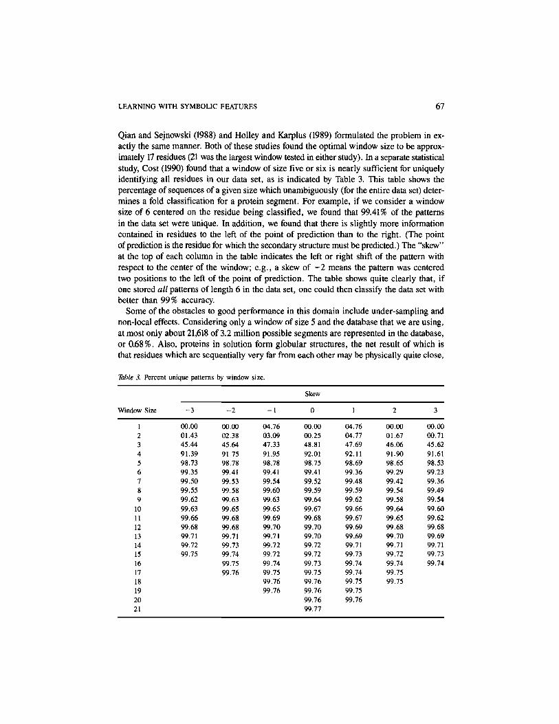
Qian and Sejnowski (1988) and Holley and Karplus (1989) formulated the problem in ex-actly the same manner. Both of these studies found the optimal window size to be approx-imately 17 residues (21 was the largest window tested in either study). In a separate statisticalstudy, Cost (1990) found that a window of size five or six is nearly sufficient for uniquelyidentifying all residues in our data set, as is indicated by Table 3. This table shows thepercentage of sequences of a given size which unambiguously (for the entire data set) deter-mines a fold classification for a protein segment. For example, if we consider a windowsize of 6 centered on the residue being classified, we found that 99.41% of the patternsin the data set were unique. In addition, we found that there is slightly more informationcontained in residues to the left of the point of prediction than to the right. (The pointof prediction is the residue for which the secondary structure must be predicted.) The "skew"at the top of each column in the table indicates the left or right shift of the pattern withrespect to the center of the window; e.g., a skew of -2 means the pattern was centeredtwo positions to the left of the point of prediction. The table shows quite clearly that, ifone stored all patterns of length 6 in the data set, one could then classify the data set withbetter than 99% accuracy.

Some of the obstacles to good performance in this domain include under-sampling andnon-local effects. Considering only a window of size 5 and the database that we are using,at most only about 21,618 of 3.2 million possible segments are represented in the database,or 0.68%. Also, proteins in solution form globular structures, the net result of which isthat residues which are sequentially very far from each other may be physically quite close,

Table 3. Percent unique patterns by window size.

Window Size

123456789

101112131415161718192021

Skew

-3

00.0001.4345.4491.3998.7399.3599.5099.5599.6299.6399.6699.6899.7199.7299.75

-2

00.0002.3845.6491.7598.7899.4199.5399.5899.6399.6599.6899.6899.7199.7399.7499.7599.76

-1

04.7603.0947.3391.9598.7899.4199.5499.6099.6399.6599.6999.7099.7199.7299.7299.7499.7599.7699.76

0

00.0000.2548.8192.0198.7599.4199.5299.5999.6499.6799.6899.7099.7099.7299.7299.7399.7599.7699.7699.7699.77

1

04.7604.7747.6992.1198.6999.3699.4899.5999.6299.6699.6799.6999.6999.7199.7399.7499.7499.7599.7599.76

2

00.0001.6746.0691.9098.6599.2999.4299.5499.5899.6499.6599.6899.7099.7199.7299.7499.7599.75

3

00.0000.7145.6291.6198.5399.2399.3699.4999.5499.6099.6299.6899.6999.7199.7399.74


and have significant effects on each other. For this reason, secondary structure probablycannot be completely determined from primary structure. Qian and Sejnowski (1988) claimthat no method incorporating only local information will perform much better than currentresults in the 60%-70% range (for non-homologous proteins).

3.2. Promoter sequences

The promoter sequence database was the subject of several recent experiments by Towell etal. (1990). Related to the protein folding task, it involves predicting whether or not a givensubsequence of a DNA sequence is a promoter—a sequence of genes that initiates a processcalled transcription, the expression of an adjacent gene. This data set contains 106 examples,53 of which are positive examples (promoters). The negative examples were generated fromlarger DNA sequences that are believed to contain no promoters. See Towell et al. (1990)for more detail on the construction of the data set. An instance consists of a sequence of57 nucleotides from the alphabet a, c, g, and t, and a classification of + or -. For learn-ing, the 57 nucleotides are treated as 57 features, each with one of four symbolic values.

3.3. Pronunciation of English text

The word-pronunciation problem presents interesting challenges for machine learning, al-though effective practical algorithms have been developed for this task. Given a relativelysmall sequence of letters, the objective is to learn the sound and stress required to pro-nounce each part of a given word. Sejnowski and Rosenberg (1987) introduced this taskto the learning community with their NETtalk program. NETtalk, which used the backpropagation learning method, performed well on this task when pronouncing both wordsand continuous spoken text, although it could not match the performance of current speechsynthesis programs.

The instance representation for text pronunciation is very similar to the previous prob-lems. Instances are sequences of letters which make up a word, and the task is to classifythe central letter in the sequence with its correct phoneme. We used a fixed window ofseven characters for our experiments, as did Sejnowski and Rosenberg. (Stanfill and Waltz(1986) used a window of size 15.) The classes include 54 phonemes plus 5 stress classifica-tions. When phoneme and stress are predicted, there are 5 x 54 = 270 possible classes,although only 115 actually occur in the dictionary. Our experiments emphasized predictionof phonemes only.

The difficulties in this domain arise from the irregularity of natural language, and theEnglish language in particular. Few rules exist that do not have exceptions. Better perfor-mance on the same data set can be obtained with (non-learning) rule-based approaches(Kontogiorgios, 1988); however, learning algorithms have trouble finding the best set of rules.

4. Experimental results

In this section, we describe our experiments and results on each of the three test domains.For comparison, we use previously published results for other learning methods. In order


to make the comparisons valid, we attempted to duplicate the experimental design of earlierstudies as closely as possible, and we used the same data as was used by those studies.

4.1. Protein secondary structure

The protein sequences used for our experiments were originally from the BrookhavenNational Laboratory. Secondary structure assignments of a-helix, 3-sheet, and coil weremade based on atomic coordinates using the method of Kabsch and Sander (1983). Qianand Sejnowski (1988) collected a database of 106 proteins, containing 128 protein segments(which they called "subunits"). We used the same set of proteins and segments that theyused. A parallel experiment by Sigillito (1989), using back propagation on the identicaldata, reproduced the classification accuracy results of Qian and Sejnowski.

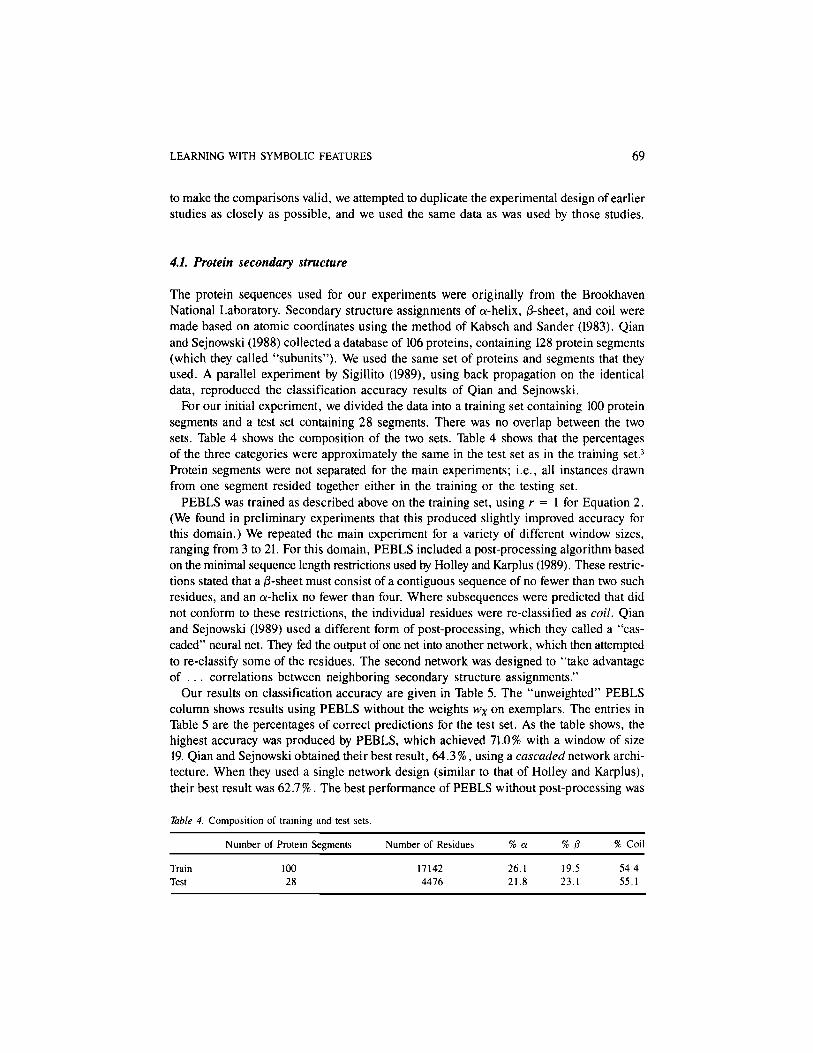
For our initial experiment, we divided the data into a training set containing 100 proteinsegments and a test set containing 28 segments. There was no overlap between the twosets. Table 4 shows the composition of the two sets. Table 4 shows that the percentagesof the three categories were approximately the same in the test set as in the training set.3

Protein segments were not separated for the main experiments; i.e., all instances drawnfrom one segment resided together either in the training or the testing set.

PEBLS was trained as described above on the training set, using r = 1 for Equation 2.(We found in preliminary experiments that this produced slightly improved accuracy forthis domain.) We repeated the main experiment for a variety of different window sizes,ranging from 3 to 21. For this domain, PEBLS included a post-processing algorithm basedon the minimal sequence length restrictions used by Holley and Karplus (1989). These restric-tions stated that a 3-sheet must consist of a contiguous sequence of no fewer than two suchresidues, and an a-helix no fewer than four. Where subsequences were predicted that didnot conform to these restrictions, the individual residues were re-classified as coil. Qianand Sejnowski (1989) used a different form of post-processing, which they called a "cas-caded" neural net. They fed the output of one net into another network, which then attemptedto re-classify some of the residues. The second network was designed to "take advantageof ... correlations between neighboring secondary structure assignments."

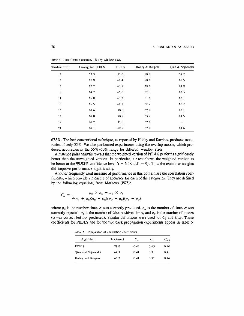
Our results on classification accuracy are given in Table 5. The "unweighted" PEBLScolumn shows results using PEBLS without the weights wx on exemplars. The entries inTable 5 are the percentages of correct predictions for the test set. As the table shows, thehighest accuracy was produced by PEBLS, which achieved 71.0% with a window of size19. Qian and Sejnowski obtained their best result, 64.3%, using a cascaded network archi-tecture. When they used a single network design (similar to that of Holley and Karplus),their best result was 62.7%. The best performance of PEBLS without post-processing was

Table 4. Composition of training and test sets.

TrainTest

Number of Protein Segments

10028

Number of Residues

171424476

% a

26.121.8

% 0

19.523.1

% Coil

54.455.1


Table 5. Classification accuracy (%) by window size.

Window Size

3

5

7

9

11

13

15

17

19

21

Unweighted PEBLS

57.5

60.9

62.7

64.7

66.0

66.5

67.6

68.0

69.2

69.1

PEBLS

57.6

61.4

63.8

65.6

67.2

68.1

70.0

70.8

71.0

69.8

Holley & Karplus

60.0

60.6

59.6

62.3

61.6

62.7

62.9

63.2

62.6

62.9

Qian & Sejnowski

57.7

60.5

61.9

62.3

62.1

62.7

62.2

61.5

-

61.6

67.8%. The best conventional technique, as reported by Holley and Karplus, produced accu-racies of only 55 %. We also performed experiments using the overlap metric, which pro-duced accuracies in the 55%-60% range for different window sizes.

A matched pairs analysis reveals that the weighted version of PEBLS performs significantlybetter than the unweighted version. In particular, a t-test shows the weighted version tobe better at the 99.95% confidence level (t = 5.48, d.f. = 9). Thus the exemplar weightsdid improve performance significantly.

Another frequently used measure of performance in this domain are the correlation coef-ficients, which provide a measure of accuracy for each of the categories. They are definedby the following equation, from Mathews (1975):

where pa is the number times a. was correctly predicted, na is the number of times a wascorrectly rejected, oa is the number of false positives for a, and ua is the number of misses(a was correct but not predicted). Similar definitions were used for C@ and Ccoil. Thesecoefficients for PEBLS and for the two back propagation experiments appear in Table 6.

Table 6. Comparison of correlation coefficients.

Algorithm

PEBLS

Qian and Sejnowski

Holley and Karplus

% Correct

71.0

64.3

63.2

ca

0.47

0.41

0.41

Cp

0.45

0.31

0.32

Ccoil

0.40

0.41

0.46


Table 7. Training PEBLS on varying percentages of the data set.

Training Set Size (%)

102030405060708090

Percent Correct on Test Set

56.157.158.759.760.260.962.363.465.1

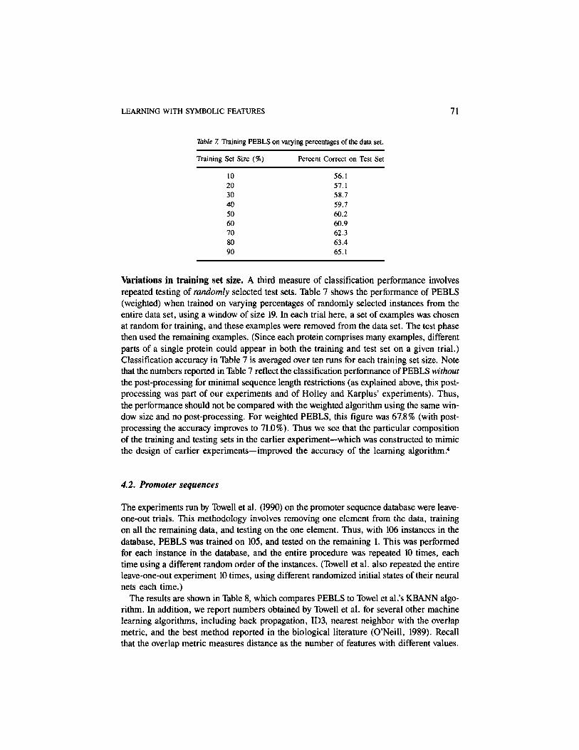
Variations in training set size. A third measure of classification performance involvesrepeated testing of randomly selected test sets. Table 7 shows the performance of PEBLS(weighted) when trained on varying percentages of randomly selected instances from theentire data set, using a window of size 19. In each trial here, a set of examples was chosenat random for training, and these examples were removed from the data set. The test phasethen used the remaining examples. (Since each protein comprises many examples, differentparts of a single protein could appear in both the training and test set on a given trial.)Classification accuracy in Table 7 is averaged over ten runs for each training set size. Notethat the numbers reported in Table 7 reflect the classification performance of PEBLS withoutthe post-processing for minimal sequence length restrictions (as explained above, this post-processing was part of our experiments and of Holley and Karplus' experiments). Thus,the performance should not be compared with the weighted algorithm using the same win-dow size and no post-processing. For weighted PEBLS, this figure was 67.8% (with post-processing the accuracy improves to 71.0%). Thus we see that the particular compositionof the training and testing sets in the earlier experiment—which was constructed to mimicthe design of earlier experiments—improved the accuracy of the learning algorithm.4

4.2. Promoter sequences

The experiments run by Towell et al. (1990) on the promoter sequence database were leave-one-out trials. This methodology involves removing one element from the data, trainingon all the remaining data, and testing on the one element. Thus, with 106 instances in thedatabase, PEBLS was trained on 105, and tested on the remaining 1. This was performedfor each instance in the database, and the entire procedure was repeated 10 times, eachtime using a different random order of the instances. (Towell et al. also repeated the entireleave-one-out experiment 10 times, using different randomized initial states of their neuralnets each time.)

The results are shown in Table 8, which compares PEBLS to Towel et al.'s KBANN algo-rithm. In addition, we report numbers obtained by Towell et al. for several other machinelearning algorithms, including back propagation, ID3, nearest neighbor with the overlapmetric, and the best method reported in the biological literature (O'Neill, 1989). Recallthat the overlap metric measures distance as the number of features with different values.


Table 8. Promoter sequence prediction.

Algorithm

PEBLSKBANNPEBLS (unweighted)Back propagationID3Nearest Neighbor (overlap)O'Neill

Error Rate

4/1064/1066/1068/106

19/10613/10612/106

It is also worth noting that in each of the 10 test runs of PEBLS, the same four instancescaused the errors, and that three of these four were negative instances. Towell notes thatthe negative examples in his database (the same data as used here) were derived by selectingsubstrings from a fragment of E. coli bacteriophage that is "believed not to contain anypromoter sites" (Towell et al., 1990). We would suggest, based on our results, that fourof the examples be re-examined. These four examples might be interesting exceptions tothe general patterns for DNA promoters.

4.3. English text pronunciation

For the English pronunciation task, we used the training set defined by Sejnowski andRosenberg (1987) for their NETtalk program. This set consists of all instances drawn fromthe Brown Corpus, or the 1000 most commonly used words of the English language. Wewere unable to discern a difference between that training set and the somewhat morerestricted set of Shavlik (Shavlik et al., 1989), so only one experimental design was used.After training on the Brown Corpus, PEBLS was tested on the entire 20,012-word MerriamWebster Pocket Dictionary. Results are presented in Table 9 for weighted and unweightedversions of the PEBLS algorithm. For comparison, we give results from the NETtalk pro-gram, which used the back propagation algorithm.

Shavlik et al. (1989) replicated Sejnowski and Rosenberg's methodology as part of theirwork, and although their results differ from Sejnowski and Rosenberg's (not surprisingly,since back propagation networks require much tuning), they make for easier comparisonwith ours. This property follows from the fact that the original Sejnowski and Rosenbergstudy used a distributed output encoding; that is, their system produced a 26-bit sequence(rather than one bit for each of the 115 phoneme/stress combinations). The first 21 bitswere a distributed encoding of the 51 phonemes, and the remaining 5 bits were a local

Table 9. English text pronunciation.

Algorithm

PEBLSPEBLS (unweighted)Back propagation

Phoneme Accuracy

78.279.1

—

Phoneme/Stress

69.267.277.0


Table 10. Phoneme/stress accuracy and output encoding.

Algorithm

PEBLSBack propagationID3Perceptron

Local Encoding(% Correct)

69.263.064.249.2

Distributed Encoding(% Correct)

72.369.342.1

Table 11. PEBLS performance on varying trainingset sizes.

Percentage of BrownCorpus for Training

510255075

100

% Phonemes Correctin Full Dictionary

60.166.272.175.877.478.2

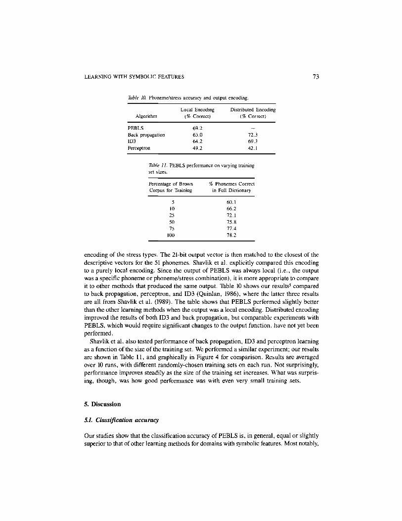
encoding of the stress types. The 21-bit output vector is then matched to the closest of thedescriptive vectors for the 51 phonemes. Shavlik et al. explicitly compared this encodingto a purely local encoding. Since the output of PEBLS was always local (i.e., the outputwas a specific phoneme or phoneme/stress combination), it is more appropriate to compareit to other methods that produced the same output. Table 10 shows our results5 comparedto back propagation, perceptron, and ID3 (Quinlan, 1986), where the latter three resultsare all from Shavlik et al. (1989). The table shows that PEBLS performed slightly betterthan the other learning methods when the output was a local encoding. Distributed encodingimproved the results of both ID3 and back propagation, but comparable experiments withPEBLS, which would require significant changes to the output function, have not yet beenperformed.

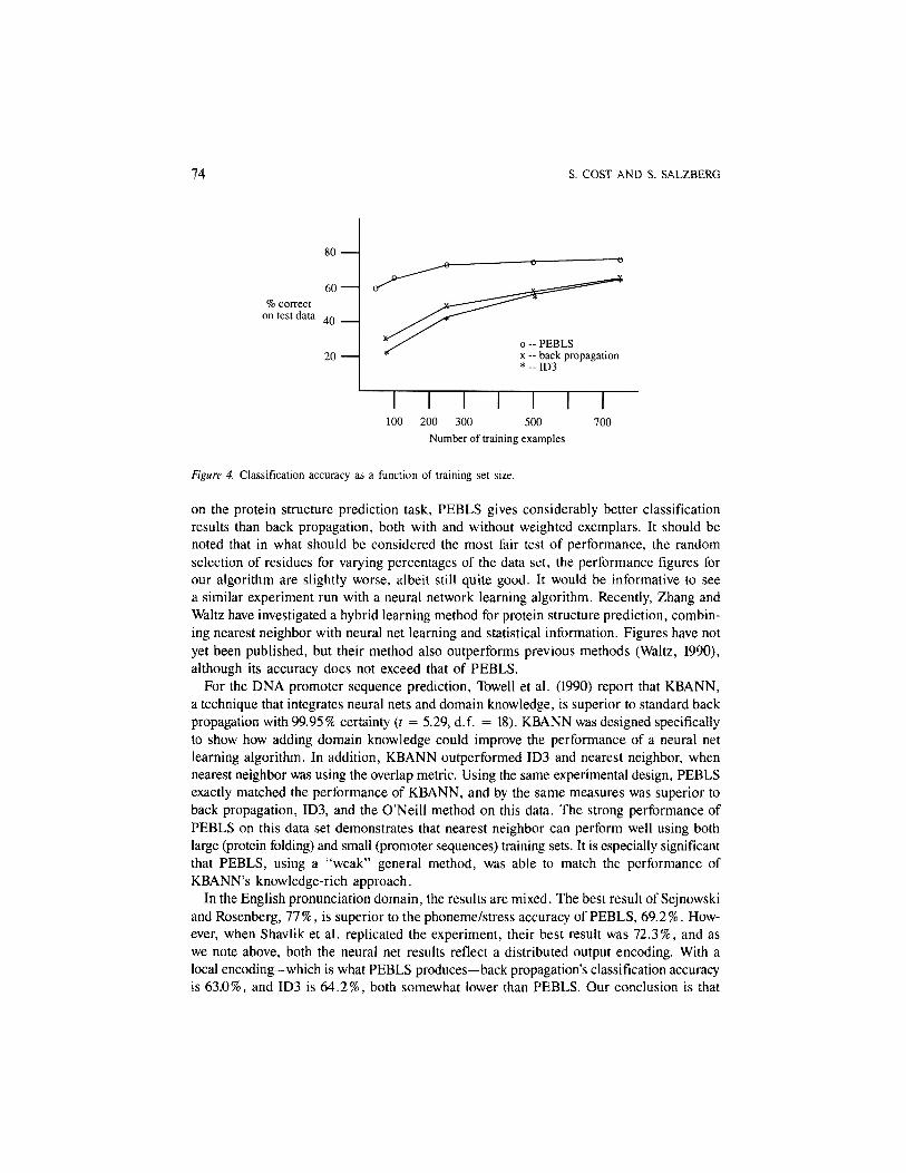
Shavlik et al. also tested performance of back propagation, ID3 and perceptron learningas a function of the size of the training set. We performed a similar experiment; our resultsare shown in Table 11, and graphically in Figure 4 for comparison. Results are averagedover 10 runs, with different randomly-chosen training sets on each run. Not surprisingly,performance improves steadily as the size of the training set increases. What was surpris-ing, though, was how good performance was with even very small training sets.

5. Discussion

5.1. Classification accuracy

Our studies show that the classification accuracy of PEBLS is, in general, equal or slightlysuperior to that of other learning methods for domains with symbolic features. Most notably,


Figure 4. Classification accuracy as a function of training set size.

on the protein structure prediction task, PEBLS gives considerably better classificationresults than back propagation, both with and without weighted exemplars. It should benoted that in what should be considered the most fair test of performance, the randomselection of residues for varying percentages of the data set, the performance figures forour algorithm are slightly worse, albeit still quite good. It would be informative to seea similar experiment run with a neural network learning algorithm. Recently, Zhang andWaltz have investigated a hybrid learning method for protein structure prediction, combin-ing nearest neighbor with neural net learning and statistical information. Figures have notyet been published, but their method also outperforms previous methods (Waltz, 1990),although its accuracy does not exceed that of PEBLS.

For the DNA promoter sequence prediction, Towell et al. (1990) report that KBANN,a technique that integrates neural nets and domain knowledge, is superior to standard backpropagation with 99.95% certainty (t = 5.29, d.f. = 18). KBANN was designed specificallyto show how adding domain knowledge could improve the performance of a neural netlearning algorithm. In addition, KBANN outperformed ID3 and nearest neighbor, whennearest neighbor was using the overlap metric. Using the same experimental design, PEBLSexactly matched the performance of KBANN, and by the same measures was superior toback propagation, ID3, and the O'Neill method on this data. The strong performance ofPEBLS on this data set demonstrates that nearest neighbor can perform well using bothlarge (protein folding) and small (promoter sequences) training sets. It is especially significantthat PEBLS, using a "weak" general method, was able to match the performance ofKBANN's knowledge-rich approach.

In the English pronunciation domain, the results are mixed. The best result of Sejnowskiand Rosenberg, 77%, is superior to the phoneme/stress accuracy of PEBLS, 69.2%. How-ever, when Shavlik et al. replicated the experiment, their best result was 72.3%, and aswe note above, both the neural net results reflect a distributed output encoding. With alocal encoding—which is what PEBLS produces—back propagation's classification accuracyis 63.0%, and ID3 is 64.2%, both somewhat lower than PEBLS. Our conclusion is that


all techniques perform similarly, and that no learning technique yet comes close to theperformance of good commercial systems, much less native speakers of English. Clearly,there is still room for considerable progress in this domain.

Shavlik et al. concluded, based on their experiments with classification accuracy versusnumber of training examples (see Figure 4 on the NETtalk data), that for small amountsof training data, back propagation was preferable to the decision trees constructed by ID3.However, our results indicate that nearest neighbor algorithms also work well when thetraining set is small. Our performance curve in Figure 4 shows that PEBLS needs veryfew examples to achieve relatively good performance.

5.2. Transparency of representation and operation

Once trained on a given domain, PEBLS contains in its memory a set of information thatis relatively perspicuous in comparison to the weight assignments of a neural network.The exemplars themselves provide specific reference instances, or "case histories" as itwere, which may be cited as support for a particular decision. Other information may easilybe gathered during the training or even the testing phase that can shed additional light onthe domain in question. For instance, consider attaching a counter to each exemplar andincrementing it each time the exemplar is used as an exact match. By comparing this withthe number of times an exemplar was used, we can get a good idea as to whether the ex-emplar is a very specific exception, or part of a very general rule. By examining the weightwx we attach to exemplars, we can determine whether the instance is a reliable classifier.The distance tables reveal an order on the set of symbolic values that is not apparent inthe values alone. On the other hand, the derivation of these distances is not perspicuous,being derived from global characteristics of the training data.

For the English pronunciation task, distributed output encodings have been shown toproduce superior performance to local encodings (Shavlik et al, 1989). This result pointsout a weakness of PEBLS, and of the 1-nearest-neighbor method, in that they do not allowfor distributed output encodings. Neural nets can handle such encodings quite easily, anddecision trees can handle them with some difficulty. (Shavlik et al. built a separate decisiontree for each of the 26 bits in the distributed encoding of the phoneme/stress pairs in thistask.) This raises the question of whether nearest neighbor methods can handle such encod-ings. One possibility is to use k-nearest neighbor, which would allow more than one exemplarto determine each of the output bits. E.g., if each exemplar contained the 26-bit encoding,the predicted value of each bit /' for a new example would be determined by the majorityvote of the k nearest neighbors for that bit. Further experiments are required to determineif such a strategy would be advantageous in general.

As for transparency of operation, the learning and classification algorithms of the nearestneighbor algorithm are very simple. The basic learning routine simply stores new examplesin memory. In PEBLS, the computation of exemplar weights is nothing more than simplerecord-keeping based on the classification performance of the existing exemplars. Addingexemplars and changing weights change the way nearest neighbor algorithms partition afeature space, as we have illustrated above with our exception spaces. Although this maybe hard to visualize in more than three dimensions, it is nonetheless straightforward.


One minor drawback is that the PEBLS method is nonincremental, unlike back propaga-tion and some versions of decision tree methods. An incremental extension to PEBLS wouldprobably be quite expensive, since the value difference tables might have to be recomputedmany times. On the other hand, extending PEBLS to handle mixed symbolic and numericdata is quite straightforward: the algorithm could use simple differences for numeric features,and value difference tables for symbolic ones.

Finally, our experiments in the protein domain demonstrated that the use of weights at-tached to exemplars can improve the accuracy of nearest neighbor algorithms. In otherdomains, such as English pronunciation, weights did not make a significant difference.Based on these results, and our earlier results on real-valued domains (Salzberg, 1990;1991), we conclude that exemplar weights offer real potential for enhancing the power ofpractical learning algorithms.

6. Conclusion

We have demonstrated, through a series of experiments, that an instance-based learningalgorithm can perform exceptionally well on domains in which features values are sym-bolic. In direct comparisons, our implementation (PEBLS) performed as well as (or betterthan) back propagation, ID3, and several domain-specific learning algorithms on severaldifficult classification tasks. In addition, nearest neighbor offers clear advantages in thatit is much faster to train and its representation relatively easy to interpret. No one yet knowshow to interpret the networks of weights learned by neural nets. Decision trees are somewhateasier to interpret, but it is hard to predict the impact of a new example on the structureof the tree. Sometimes one new example makes no difference at all, and at other timesit may radically change a large portion of the tree. On the other hand, neural nets havea fixed size, and decision trees tend to be quite small, and in this respect both methodscompress the data in a way that nearest neighbor does not. In addition, classification timeis fast (dependent only on the depth of the net or tree, not on the size of the input). Basedon classification accuracy, though, it is not clear that other learning techniques have anadvantage over nearest-neighbor methods.

With respect to nearest neighbor learning per se, we have shown how weighting exemplarscan improve performance by subdividing the instance space in a manner that reduces theimpact of unreliable examples. The nearest neighbor algorithm is one of the simplest learn-ing methods known, and yet no other algorithm has been shown to outperform it consistently.Taken together, these results indicate that continued research on extending and improvingnearest neighbor learning algorithms should prove fruitful.

Acknowledgments

Thanks to Joanne Houlahan and David Aha for numerous insightful comments and sugges-tions. Thanks also to Richard Sutton and three anonymous reviewers for their detailedcomments and ideas. This research was supported in part by the Air Force Office of Scien-tific Research under Grant AFOSR-89-0151, and by the National Science Foundation underGrant IRI-9116843.


Notes

1. For reference, the system takes about 30 minutes of real time on a DECstation 3100 to train on 17,142 instances.The experimenter's time is limited to a few minutes defining the data set.

2. The parallelization of the algorithm was developed to speed up experimentation, and is of no theoretical impor-tance to our learning model.

3. Qian and Sejnowski carefully balanced the overall frequencies of the three categories in the training and testsets, and we attempted to do the same. In addition, they used a training set with 18,105 residues, while ourswas slightly smaller. Although our databases were identical, we did not have access to the specific partitioninginto training and test sets used by Qian and Sejnowski.

4. One likely source of variation in classification accuracy is homologies between the training and test sets. Homo-logous proteins are structurally very similar, and an algorithm may be much more accurate at predicting thestructure of a protein once it has been trained on a homologous one.

5. In our preliminary experiments, we used the overlap metric on this database, with abysmal results. Our desireto improve these results was one of the reasons we developed the MVDM.

References

Aha, D. (1989). Incremental, instance-based learning of independent and graded concept descriptions. Proceedingsof the Sixth International Workshop on Machine Learning (pp. 387-391). Ithaca, NY: Morgan Kaufmann.

Aha, D. & Kibler, D. (1989). Noise-tolerant instance-based learning algorithms. Proceedings of the Eleventh Inter-national Joint Conference on Artificial Intelligence (p. 794-799). Detroit, MI: Morgan Kaufmann.

Aha, D. (1990). A study of instance-based algorithms for supervised learning tasks. Doctoral dissertation, Departmentof Information and Computer Science, University of California, Irvine. Technical Report 90-42.

Aha, D., Kibler, D., & Albert, M. (1991). Instance-based learning algorithms. Machine Learning, 6(1) 37-66.Chou, P. & Fasman, G. (1978). Prediction of the secondary structure of proteins from their amino acid sequence.

Advanced Enzymology, 47 , 45-148. Biochemistry, 13, 222-245.Cohen, F, Abarbanel, R., Kuntz, I., & Fletterick, R. (1986). Turn prediction in proteins using a pattern match-

ing approach. Biochemistry, 25, 266-275.Cost, S. (1990). Master's thesis, Department of Computer Science, Johns Hopkins University.Cost, S. & Salzberg, S. (1990). Exemplar-based learning to predict protein folding. Proceedings of the Symposium

on Computer Applications to Medical Care (pp. 114-118). Washington, DC.Cover, T. & Hart, P. (1967). Nearest neighbor pattern classification. IEEE Transactions on Information Theory,

13(1), 21-27.Crick, F. & Asanuma, C. (1986). Certain aspects of the anatomy and physiology of the cerebral cortex. In J.

McClelland, D. Rumelhart, & the PDP Research Group (Eds.), Parallel distributed processing: Explorationsin the microstructure of cognition (Vol. II). Cambridge, MA: MIT Press.

Dietterich, T., Hild, H., & Bakiri, G. (1990). A comparative study of ID3 and backpropagation for English text-to-speech mapping. Proceedings of the 7th International Conference on Machine Learning (pp. 24-31), SanMateo, CA: Morgan Kaufmann.

Fertig, S. & Gelernter, D. (1991). FGP: A virtual machine for acquiring knowledge from cases. Proceedings ofthe 12th International Joint Conference on Artificial Intelligence (pp. 796-802). Los Altos, CA: Morgan Kaufmann.

Fisher, D. & McKusick, K. (1989). An empirical comparison of ID3 and backpropagation. Proceedings of theInternational Joint Conference on Artificial Intelligence (pp. 788-793) San Mateo, CA: Morgan Kaufmann.

Garnier, J., Osguthorpe, D., & Robson, B. (1978). Analysis of the accuracy and implication of simple methodsfor predicting the secondary structure of globular proteins. Journal of Molecular Biology, 120, 97-120.

Hanson, S. & Burr, D. (1990). What connectionist models learn: Learning and representation in connectionistnetworks. Behavioral and Brain Sciences, 13 471-518.

Holley, L. & Karplus, M. (1989). Protein secondary structure prediction with a neural network. Proceedingsof the National Academy of Sciences USA, 86, 152-156.

Kabsch, W. & Sander, C. (1983). Dictionary of protein secondary structure: Pattern recognition of hydrogen-bonded and geometric features. Biopolymers, 22, 2577-2637.


Kontogiorgis, S. (1988). Automatic letter-to-phoneme transcription for speech synthesis (Technical ReportJHU-88/22). Department of Computer Science, Johns Hopkins University.

Lathrop, R., Webster, T., & Smith, T. (1987). ARIADNE: Pattern-directed inference and hierarchical abstractionin protein structure recognition. Communications of the ACM, 30(11), 909-921.

Lim, V. (1974). Algorithms for prediction of alpha-helical and be fa-structural regions in globular proteins. Journalof Molecular Biology, 88, 873-894.

Mathews, B.W. (1975). Comparison of the predicted and observed secondary structure of T4 phage lysozyme.Biochimica et Biophysica Acta, 405, 442-451.

McClelland, J. & Rumelhart, D. (1986). A distributed model of human learning and memory. In J. McClelland,D. Rumelhart, & the PDP Research Group (Eds.), Parallel distributed processing: Explorations in the microstruc-ture of cognition (Vol. II). Cambridge, MA: MIT Press.

Medin, D. & Schaffer, M. (1978). Context theory of classification learning. Psychological Review, 85(3) 207-238.Mooney, R., Shavlik, J., Towell, G., & Gove, A. (1989). An experimental comparison of symbolic and connec-

tionist learning algorithms. Proceedings of the International Joint Conference on Artificial Intelligence (pp.775-780). San Mateo, CA: Morgan Kaufmann.

Nosofsky, R. (1984). Choice, similarity, and the context theory of classification. Journal of Experimental Psychology:Learning, Memory, and Cognition 10(1), 104-114.

O'Neill, M. (1989). Escherichia coli promoters: I. Consensus as it relates to spacing class, specificity, repeatsubstructure, and three dimensional organization. Journal of Biological Chemistry, 264, 5522-5530.

Preparata, F. & Shamos, M. (1985). Computational geometry: An introduction. New York: Springer-Verlag.Qian, N. & Sejnowski, T. (1988). Predicting the secondary structure of globular proteins using neural network

models. Journal of Molecular Biology, 202, 865-884.Reed, S. (1972). Pattern recognition and categorization. Cognitive Psychology, 3, 382-407.Rumelhart, D., Hinton, G., & Williams, R. (1986). Learning representations by backpropagating errors. Nature,

323(9), 533-536.Rumelhart, D., Smolensky, P., McClelland, J., & Hinton, G. (1986). Schemata and sequential thought processes

in PDP models. In J. McClelland, D. Rumelhart, & the PDP Research Group (Eds.), Parallel distributed proc-essing: Explorations in the microstructure of cognition (Vol. II). Cambridge, MA: MIT Press.

Rumelhart, D., McClelland, J., & the PDP Research Group (1986). Parallel distributed processing: Explorationsin the microstructure of cognition (Vol. I). Cambridge, MA: MIT Press.

Salzberg, S. (1989). Nested hyper-rectangles for exemplar-based learning. In K.P. Jantke (Ed.), Analogical andInductive Inference: International Workshop All '89. Berlin: Springer-Verlag.

Salzberg, S. (1990). Learning with nested generalized exemplars. Norwell, MA: Kluwer Academic Publishers.Salzberg, S. (1991). A nearest hyperrectangle learning method. Machine Learning, 6(3), 251-276.Sejnowski, T. & Rosenberg, C. (1987). NETtalk: A parallel network that learns to read aloud. Complex Systems,

1 145-168. (Also Technical Report JHU/EECS-86/01. Baltimore, MD: John Hopkins University.Shavlik, J., Mooney, R., & Towell, G. (1989). Symbolic and neural learning algorithms: an experimental com-

parison (Technical Report #857). Madison, WI: Computer Sciences Department, University of Wisconsin.Sigillito, V. (1989). Personal communication.Stanfill, C. & Waltz, D. (1986). Toward memory-based reasoning. Communications of the ACM, 29(12), 1213-1228.Towell, G., Shavlik, J., & Noordewier, M. (1990). Refinement of approximate domain theories by knowledge-

based neural networks. Proceedings Eighth National Conference on Artificial Intelligence (pp. 861-866). MenloPark, CA: AAAI Press.

Waltz, D. (1990). Massively parallel AI. Proceedings Eighth National Conference on Artificial Intelligence (pp.1117-1122). Menlo Park, CA: AAAI Press.

Weiss, S. & Kapouleas, I. (1989). An empirical comparison of pattern recognition, neural nets, and machinelearning classification methods. Proceedings of the International Joint Conference on Artificial Intelligence(pp. 781-787). San Mateo, CA: Morgan Kaufmann.

Received October 9, 1990Accepted June 14, 1991Final Manuscript January 21, 1992

a weighted nearest neighbor algorithm for learning with ...1022664626993.pdf · a weighted nearest...

Documents