a verification framework for hybrid systems
TRANSCRIPT
A Verification Framework for Hybrid Systems
Sayan Mitra
September 2007
32 VASSAR STREET, CAMBRIDGE, MASSACHUSETTS 02139
COMPUTER SCIENCE AND ARTIFICIAL INTELLIGENCE LABORATORY
MASSACHUSETTS INSTITUTE OF TECHNOLOGY

A Verification Framework for Hybrid Systems
by
Sayan Mitra
Submitted to the Department of Electrical Engineering and Computer Sciencein partial fulfillment of the requirements for the degree of
Doctor of Philosophy
at the
MASSACHUSETTS INSTITUTE OF TECHNOLOGY
September 2007
© Massachusetts Institute of Technology 2007. All rights reserved.
Author . . . . . . . . . . . . . . . . . . . . . . . . . . . . . . . . . . . . . . . . . . . . . . . . . . . . . . . . . . . . . . . . . . . . . . . . . . . .Department of Electrical Engineering and Computer Science
August 31, 2007
Certified by. . . . . . . . . . . . . . . . . . . . . . . . . . . . . . . . . . . . . . . . . . . . . . . . . . . . . . . . . . . . . . . . . . . . . . . .Nancy A. Lynch
NEC Professor of Software Science and EngineeringThesis Supervisor
Accepted by . . . . . . . . . . . . . . . . . . . . . . . . . . . . . . . . . . . . . . . . . . . . . . . . . . . . . . . . . . . . . . . . . . . . . . .Arthur C. Smith
Chairman, Department Committee on Graduate Students
A Verification Framework for Hybrid Systemsby
Sayan Mitra
Submitted to the Department of Electrical Engineering and Computer Scienceon August 31, 2007, in partial fulfillment of the
requirements for the degree ofDoctor of Philosophy
Abstract
Combining discrete state transitions with differential equations, Hybrid system models pro-vide an expressive formalism for describing software systems that interact with a physicalenvironment. Automatically checking properties, such as invariance and stability, is ex-tremely hard for general hybrid models, and therefore current research focuses on modelswith restricted expressive power. In this thesis we take a complementary approach by de-veloping proof techniques that are not necessarily automatic, but are applicable to a generalclass of hybrid systems. Three components of this thesis, namely, (i) semantics for ordi-nary and probabilistic hybrid models, (ii) methods for proving invariance, stability, andabstraction, and (iii) software tools supporting (i) and (ii), are integrated within a commonmathematical framework.
(i) For specifying nonprobabilistic hybrid models, we present Structured Hybrid I/O Au-tomata (SHIOAs) which adds control theory-inspired structures, namely state models,to the existing Hybrid I/O Automata, thereby facilitating description of continuous be-havior. We introduce a generalization of SHIOAs which allows both nondeterministicand stochastic transitions and develop the trace-based semantics for this framework.
(ii) We present two techniques for establishing lower-bounds on average dwell time (ADT)for SHIOA models. This provides a sufficient condition of establishing stability forSHIOAs with stable state models. A new simulation-based technique which is soundfor proving ADT-equivalence of SHIOAs is proposed.
We develop notions of approximate implementation and corresponding proof tech-niques for Probabilistic I/O Automata. Specifically, a PIOA A is an ε-approximateimplementation of B, if every trace distribution of A is ε-close to some trace distribu-tion of B—closeness being measured by a metric on the space of trace distributions.We present a new class of real-valued simulation functions for proving ε-approximateimplementations, and demonstrate their utility in quantitatively reasoning about prob-abilistic safety and termination.
(iii) We introduce a specification language for SHIOAs and a theorem prover interface forthis language. The latter consists of a translator to typed high order logic and a setof PVS-strategies that partially automate the above verification techniques within thePVS theorem prover.
Thesis Supervisor: Nancy A. LynchTitle: NEC Professor of Software Science and Engineering
2

Acknowledgments
I am grateful to have had Nancy Lynch as my advisor. She shared her wisdom with meand gave me freedom to explore my interests. Her enthusiasm about my ideas, blendedwith her perfectionism made for a stimulating research environment. Nancy has profoundlyinfluenced the problems I choose to work on, how I go about doing research, and theaesthetics of how I present my solutions.
It has been a pleasure to discuss my work with Sanjoy Mitter. Sanjoy shaped mythinking on probabilistic hybrid systems and encouraged me to take courses that provedto be extremely useful. I have gained from sketching my ideas to him on the blackboardand also from discussing general research directions. A significant portion of this work hasbenefited from bringing ideas from control theory into formal verification. This has beenpossible because of Daniel Liberzon’s help and guidance. I am also grateful to Daniel forbeing a delightfully supportive colleague and for providing precise, timely and reasonedfeedback.
A special thanks to Daniel Jackson for reading the thesis; your probing questions helpedme improve the presentation. I would like to acknowledge Piotr Indyk, Madhu Sudan, andRonitt Rubinfeld for being available for both academic and personal counsel, always; Piotr,even at unearthly hours. The theorem prover connection is based on my collaboration withMyla Archer. I thank her for sharing her knowledge, experience, and insights. I thank themembers of Tempo research group: Alex Shvartsman, Radu Grosu, Scott Smolka, LaurentMichel. I would like to thank Joanne Hanley and Be Blackburn for everything that youhave done to make things smooth for us—the proposals, the letters, the corn, the cookies,and yes, the moral support.
A defining feature of my MIT experience is the interaction with truly exceptionalpost-docs and fellow students. The company of Vineet Sinha, Tina Nolte, Seth Gilbert,Calvin Newport, Xavier Koegler, Ben Leong, Han-Pang Chiu, Dah-Yoh Lim, Vinod Vaikun-tanathan, Victor Chen, Roger Khazan, Carl Livadas, and Yong Wang, has been stimulatingand enjoyable. I am grateful for the support of Dilsun Kaynar in my early days, when shepatiently listened to and commented on many of my half-baked ideas. My work with ju-nior colleagues, Shinya Umeno and Hongping Lim, has been uniquely rewarding and hascontributed to the thesis. Ling Cheung deserves special mention as a formidable colleagueand for quietly suffering numerous practice talks. A special thanks to Rui Fan for manystimulating technical discussions which have influenced my thinking as a researcher, andalso for introducing me to the music of Jascha Heifetz. Thanks to my dear friend DavidHuynh for the endless hours of fun we had together.
I have the deepest gratitude to my family for their love and kindness. The support,encouragement, and the occasional nudge (to finish) from my parents, Tapan and Mamata,has been crucial for this thesis. Your wisdom and compassion continue to astonish andinspire me. I am grateful to my sister, Shreya, for being such an unwavering champion; tak-ing on this journey with you has been singularly rewarding. Finally, to my wife Shinjinee,for support, for keeping it colorful, for giving me time and space to think, and for being aconstant source of happiness—thank you.
Sayan Mitra31st August 2007, Cambridge, MA.
3
Contents
1 Introduction 101.1 Modeling and Verification of Embedded Software . . . . . . . . . . . . . . . 101.2 Hybrid Systems . . . . . . . . . . . . . . . . . . . . . . . . . . . . . . . . . . 111.3 Thesis Overview . . . . . . . . . . . . . . . . . . . . . . . . . . . . . . . . . 13
1.3.1 Modeling . . . . . . . . . . . . . . . . . . . . . . . . . . . . . . . . . 131.3.2 Verification . . . . . . . . . . . . . . . . . . . . . . . . . . . . . . . . 151.3.3 Software Tools . . . . . . . . . . . . . . . . . . . . . . . . . . . . . . 161.3.4 Reading the Thesis . . . . . . . . . . . . . . . . . . . . . . . . . . . . 17
1.4 Related Work . . . . . . . . . . . . . . . . . . . . . . . . . . . . . . . . . . . 18
I Non-probabilistic Hybrid Systems 21
2 Interactive State Machines 222.1 Preliminaries . . . . . . . . . . . . . . . . . . . . . . . . . . . . . . . . . . . 222.2 Hybrid Automata . . . . . . . . . . . . . . . . . . . . . . . . . . . . . . . . . 25
2.2.1 Definition of Hybrid Automata . . . . . . . . . . . . . . . . . . . . . 252.2.2 Executions and Traces . . . . . . . . . . . . . . . . . . . . . . . . . . 262.2.3 Composition of HA . . . . . . . . . . . . . . . . . . . . . . . . . . . . 27
2.3 Hybrid Input/Output Automata . . . . . . . . . . . . . . . . . . . . . . . . 282.3.1 Composition of HIOA . . . . . . . . . . . . . . . . . . . . . . . . . . 29
2.4 Structured Hybrid I/O Automata . . . . . . . . . . . . . . . . . . . . . . . . 302.4.1 State models . . . . . . . . . . . . . . . . . . . . . . . . . . . . . . . 302.4.2 Definition of Structured HIOA . . . . . . . . . . . . . . . . . . . . . 332.4.3 Some Special Classes of SHIOAs . . . . . . . . . . . . . . . . . . . . 352.4.4 Composition of SHIOA . . . . . . . . . . . . . . . . . . . . . . . . . 352.4.5 Summary . . . . . . . . . . . . . . . . . . . . . . . . . . . . . . . . . 37
3 The HIOA Language 383.1 An Overview . . . . . . . . . . . . . . . . . . . . . . . . . . . . . . . . . . . 383.2 Variables . . . . . . . . . . . . . . . . . . . . . . . . . . . . . . . . . . . . . 39
3.2.1 Built-in Types . . . . . . . . . . . . . . . . . . . . . . . . . . . . . . 403.2.2 Vocabularies . . . . . . . . . . . . . . . . . . . . . . . . . . . . . . . 403.2.3 Dynamic Types . . . . . . . . . . . . . . . . . . . . . . . . . . . . . . 413.2.4 Initial Values . . . . . . . . . . . . . . . . . . . . . . . . . . . . . . . 42
3.3 Functions . . . . . . . . . . . . . . . . . . . . . . . . . . . . . . . . . . . . . 433.4 Signature . . . . . . . . . . . . . . . . . . . . . . . . . . . . . . . . . . . . . 43
4

3.5 Transitions . . . . . . . . . . . . . . . . . . . . . . . . . . . . . . . . . . . . 443.5.1 Preconditions . . . . . . . . . . . . . . . . . . . . . . . . . . . . . . . 443.5.2 Effects . . . . . . . . . . . . . . . . . . . . . . . . . . . . . . . . . . . 45
3.6 Trajectories . . . . . . . . . . . . . . . . . . . . . . . . . . . . . . . . . . . . 453.6.1 Invariant Condition . . . . . . . . . . . . . . . . . . . . . . . . . . . 463.6.2 Stopping condition . . . . . . . . . . . . . . . . . . . . . . . . . . . . 463.6.3 DAIs . . . . . . . . . . . . . . . . . . . . . . . . . . . . . . . . . . . . 47
3.7 Operations and Properties . . . . . . . . . . . . . . . . . . . . . . . . . . . . 493.7.1 Composition . . . . . . . . . . . . . . . . . . . . . . . . . . . . . . . 493.7.2 Property Assertions . . . . . . . . . . . . . . . . . . . . . . . . . . . 50
3.8 Summary . . . . . . . . . . . . . . . . . . . . . . . . . . . . . . . . . . . . . 52
4 Verifying Safety Properties 534.1 An Overview . . . . . . . . . . . . . . . . . . . . . . . . . . . . . . . . . . . 534.2 Proving Invariants . . . . . . . . . . . . . . . . . . . . . . . . . . . . . . . . 544.3 Proving Implementation Relations . . . . . . . . . . . . . . . . . . . . . . . 554.4 Case Study: Safety Verification of Helicopter Testbed . . . . . . . . . . . . 56
4.4.1 System Specification . . . . . . . . . . . . . . . . . . . . . . . . . . . 574.4.2 Safety Verification . . . . . . . . . . . . . . . . . . . . . . . . . . . . 634.4.3 Preliminary Properties . . . . . . . . . . . . . . . . . . . . . . . . . . 654.4.4 User Mode . . . . . . . . . . . . . . . . . . . . . . . . . . . . . . . . 664.4.5 Supervisor Mode . . . . . . . . . . . . . . . . . . . . . . . . . . . . . 68
4.5 Summary . . . . . . . . . . . . . . . . . . . . . . . . . . . . . . . . . . . . . 74
5 Verifying Stability Properties 755.1 Assumptions . . . . . . . . . . . . . . . . . . . . . . . . . . . . . . . . . . . 755.2 Stability and Average Dwell Time . . . . . . . . . . . . . . . . . . . . . . . 76
5.2.1 Stability Definitions . . . . . . . . . . . . . . . . . . . . . . . . . . . 765.2.2 ADT Theorem of Heshpanha and Morse . . . . . . . . . . . . . . . . 77
5.3 An Overview . . . . . . . . . . . . . . . . . . . . . . . . . . . . . . . . . . . 795.4 ADT Equivalence . . . . . . . . . . . . . . . . . . . . . . . . . . . . . . . . . 805.5 Verifying ADT: Invariant approach . . . . . . . . . . . . . . . . . . . . . . . 82
5.5.1 Transformations for ADT verification . . . . . . . . . . . . . . . . . 825.5.2 Case Study: Leaking Gas-burner . . . . . . . . . . . . . . . . . . . . 855.5.3 Case Study: Scale-independent Hysteresis Switch . . . . . . . . . . . 86
5.6 Verifying ADT: Optimization-based Approach . . . . . . . . . . . . . . . . . 895.6.1 One-clock Initialized SHIOA . . . . . . . . . . . . . . . . . . . . . . 905.6.2 Case Study: Linear Hysteresis Switch . . . . . . . . . . . . . . . . . 915.6.3 Initialized SHIOA . . . . . . . . . . . . . . . . . . . . . . . . . . . . 965.6.4 MILP formulation of OPT(τa) . . . . . . . . . . . . . . . . . . . . . 985.6.5 Case Study: Thermostat . . . . . . . . . . . . . . . . . . . . . . . . . 100
5.7 Summary . . . . . . . . . . . . . . . . . . . . . . . . . . . . . . . . . . . . . 102
6 Mechanizing Proofs 1046.1 An Overview . . . . . . . . . . . . . . . . . . . . . . . . . . . . . . . . . . . 1046.2 Translation . . . . . . . . . . . . . . . . . . . . . . . . . . . . . . . . . . . . 107
6.2.1 Assumptions . . . . . . . . . . . . . . . . . . . . . . . . . . . . . . . 1076.2.2 Types and Vocabularies . . . . . . . . . . . . . . . . . . . . . . . . . 108
5

6.2.3 Variables and Initial States . . . . . . . . . . . . . . . . . . . . . . . 1096.2.4 Trajectory Types . . . . . . . . . . . . . . . . . . . . . . . . . . . . . 1096.2.5 Actions, State Models, and Moves . . . . . . . . . . . . . . . . . . . 1106.2.6 Transitions . . . . . . . . . . . . . . . . . . . . . . . . . . . . . . . . 1116.2.7 Trajectories . . . . . . . . . . . . . . . . . . . . . . . . . . . . . . . . 1136.2.8 Invariants . . . . . . . . . . . . . . . . . . . . . . . . . . . . . . . . . 1176.2.9 Simulation Relations . . . . . . . . . . . . . . . . . . . . . . . . . . . 119
6.3 Strategies . . . . . . . . . . . . . . . . . . . . . . . . . . . . . . . . . . . . . 1226.3.1 Strategies for Proving Invariants . . . . . . . . . . . . . . . . . . . . 1236.3.2 Strategies for Proving Forward Simulation . . . . . . . . . . . . . . . 125
6.4 Discussion of Case Studies . . . . . . . . . . . . . . . . . . . . . . . . . . . . 1296.4.1 Failure Detector . . . . . . . . . . . . . . . . . . . . . . . . . . . . . 1296.4.2 Two-Task Race . . . . . . . . . . . . . . . . . . . . . . . . . . . . . . 130
6.5 Summary . . . . . . . . . . . . . . . . . . . . . . . . . . . . . . . . . . . . . 131
II Probabilistic Hybrid Systems 133
7 Probabilistic State Machines 1347.1 An Overview . . . . . . . . . . . . . . . . . . . . . . . . . . . . . . . . . . . 1347.2 Preliminaries . . . . . . . . . . . . . . . . . . . . . . . . . . . . . . . . . . . 1367.3 Task-Deterministic Probabilistic Timed I/O Automata . . . . . . . . . . . . 137
7.3.1 Definition of Task DPTIOAs . . . . . . . . . . . . . . . . . . . . . . 1377.3.2 Executions and Traces . . . . . . . . . . . . . . . . . . . . . . . . . . 1407.3.3 Composition of Task-DPTIOAs . . . . . . . . . . . . . . . . . . . . . 141
7.4 Probabilistic Semantics for Task-DPTIOAs . . . . . . . . . . . . . . . . . . 1427.4.1 Semi-ring on Executions and Traces . . . . . . . . . . . . . . . . . . 1437.4.2 Probability Measure Over Executions . . . . . . . . . . . . . . . . . 1457.4.3 Probability Measure Over Traces . . . . . . . . . . . . . . . . . . . . 147
7.5 Implementation and Compositionality . . . . . . . . . . . . . . . . . . . . . 1517.6 PTIOAs and Local Schedulers . . . . . . . . . . . . . . . . . . . . . . . . . . 1527.7 A Language for Specifying PTIOAs . . . . . . . . . . . . . . . . . . . . . . . 1537.8 Summary . . . . . . . . . . . . . . . . . . . . . . . . . . . . . . . . . . . . . 157
8 Verifying Approximate Implementation Relations 1588.1 An Overview . . . . . . . . . . . . . . . . . . . . . . . . . . . . . . . . . . . 1588.2 Task-structured PIOA . . . . . . . . . . . . . . . . . . . . . . . . . . . . . . 160
8.2.1 Definition of Task Structured PIOA . . . . . . . . . . . . . . . . . . 1608.2.2 Executions and Traces . . . . . . . . . . . . . . . . . . . . . . . . . . 1618.2.3 Composition of Task-PIOAs . . . . . . . . . . . . . . . . . . . . . . . 1618.2.4 Probabilistic Executions and Trace Distributions . . . . . . . . . . . 1628.2.5 Exact implementations and Simulations . . . . . . . . . . . . . . . . 163
8.3 Uniform Approximate Implementation . . . . . . . . . . . . . . . . . . . . . 1658.3.1 Uniform Metric on Traces . . . . . . . . . . . . . . . . . . . . . . . . 1658.3.2 Expanded Approximate Simulations . . . . . . . . . . . . . . . . . . 1668.3.3 Soundness of Expanded Approximate Simulations . . . . . . . . . . 1698.3.4 Need for Expansion . . . . . . . . . . . . . . . . . . . . . . . . . . . 1738.3.5 Probabilistic Safety . . . . . . . . . . . . . . . . . . . . . . . . . . . . 176
6

8.4 Discounted Uniform Approximate Implementation . . . . . . . . . . . . . . 1768.4.1 Discounted Uniform Metric on Traces . . . . . . . . . . . . . . . . . 1778.4.2 Discounted Approximate Simulation . . . . . . . . . . . . . . . . . . 1798.4.3 Soundness of Discounted Approximate Simulation . . . . . . . . . . 179
8.5 Approximations for Task-PIOAs . . . . . . . . . . . . . . . . . . . . . . . . 1818.6 Related Work . . . . . . . . . . . . . . . . . . . . . . . . . . . . . . . . . . . 1818.7 Summary . . . . . . . . . . . . . . . . . . . . . . . . . . . . . . . . . . . . . 1828.8 Appendix: Limits of Chains of Distributions . . . . . . . . . . . . . . . . . . 183
9 Conclusions 1849.1 Evaluation . . . . . . . . . . . . . . . . . . . . . . . . . . . . . . . . . . . . . 1849.2 Future Directions . . . . . . . . . . . . . . . . . . . . . . . . . . . . . . . . . 185
9.2.1 Modeling Probabilistic Hybrid Systems . . . . . . . . . . . . . . . . 1859.2.2 Stability . . . . . . . . . . . . . . . . . . . . . . . . . . . . . . . . . . 1869.2.3 Approximate Implementations . . . . . . . . . . . . . . . . . . . . . 1879.2.4 Software Tools . . . . . . . . . . . . . . . . . . . . . . . . . . . . . . 187
List of Symbols and Functions 188
Index 190
Bibliography 193
7
List of Figures
2-1 Example of trajectories of a real-valued continuous variable. . . . . . . . . . 242-2 Hybrid automaton model of a vehicle and a typical execution. . . . . . . . . 262-3 Composition of Vehicle and Controller. . . . . . . . . . . . . . . . . . . . . . 28
3-1 Bouncing ball: HIOA specification and an execution. . . . . . . . . . . . . . . 393-2 Vocabulary for graphs. . . . . . . . . . . . . . . . . . . . . . . . . . . . . . . 413-3 Periodically sending process. . . . . . . . . . . . . . . . . . . . . . . . . . . 463-4 Thermostat. . . . . . . . . . . . . . . . . . . . . . . . . . . . . . . . . . . . . 483-5 Time-bounded channel. . . . . . . . . . . . . . . . . . . . . . . . . . . . . . 483-6 Process participating in a clock synchronization algorithm. . . . . . . . . . 493-7 Failure detector specification. . . . . . . . . . . . . . . . . . . . . . . . . . . 503-8 Periodic sender and simple failure detector. . . . . . . . . . . . . . . . . . . 513-9 Composed automaton and property assertions. . . . . . . . . . . . . . . . . 51
4-1 Helicopter testbed manufactured by Quanser Inc. . . . . . . . . . . . . . . . 574-2 Interconnection of SHIOA components in Quanser helicopter system. . . . . 584-3 Quanser helicopter pitch dynamics. . . . . . . . . . . . . . . . . . . . . . . . 584-4 Periodic noisy sensor. . . . . . . . . . . . . . . . . . . . . . . . . . . . . . . 594-5 An arbitrary user-defined controller. . . . . . . . . . . . . . . . . . . . . . . 604-6 Switching regions of supervisory controller. . . . . . . . . . . . . . . . . . . 614-7 Switched supervisory controller for helicopter testbed. . . . . . . . . . . . . 624-8 Actuator with delay. . . . . . . . . . . . . . . . . . . . . . . . . . . . . . . . 624-9 Left:At regions between U and R, Right:Bt regions between R and C. . . . 67
5-1 Leaking gas burner. . . . . . . . . . . . . . . . . . . . . . . . . . . . . . . . 855-2 Scale-independent hysteresis switch. . . . . . . . . . . . . . . . . . . . . . . 875-3 Transformed hysteresis switch. . . . . . . . . . . . . . . . . . . . . . . . . . 875-4 One-clock initialized SHIOA Aut(G) defined by directed graph G. . . . . . . 905-5 Linear hysteresis switch. . . . . . . . . . . . . . . . . . . . . . . . . . . . . . 925-6 ADT-equivalent graph (m = 3) for LinHSwitch. . . . . . . . . . . . . . . . . 935-7 Generic rectangular initialized SHIOA. . . . . . . . . . . . . . . . . . . . . . 985-8 Objective function and constraints for MOPT(K, τa) . . . . . . . . . . . . . 995-9 Thermostat2 SHIOA and its rectangular initialized abstraction ThermAbs. . 101
6-1 directedGraphs vocabulary in HIOA translated to directedGraphs theory in PVS.1096-2 Variable declarations in HIOA translated to type declarations in PVS . . . . . 1106-3 Actions and State models in HIOA translated to Moves in PVS . . . . . . . . 1116-4 Discrete transitions in HIOA and their PVS translation. . . . . . . . . . . . . 1136-5 Bounce automaton translated to Bounce theory in PVS. . . . . . . . . . . . 114
8

6-6 Spec of Figure 3-7 translated to Spec decls theory. . . . . . . . . . . . . . . 1166-7 Timeout automaton in HIOA . . . . . . . . . . . . . . . . . . . . . . . . . . . 1176-8 Timeout of Figure 6-7 translated to Timeout decls theory. . . . . . . . . . . 1186-9 Translation of invariant assertions for Timeout. . . . . . . . . . . . . . . . . 1196-10 SHIOA PVS theory. . . . . . . . . . . . . . . . . . . . . . . . . . . . . . . . 1206-11 Forward simulation theory. . . . . . . . . . . . . . . . . . . . . . . . . . . . 1226-12 Translation of forward simulation relation of failure detector. . . . . . . . . 1236-13 Base case sequent of simulation proof. . . . . . . . . . . . . . . . . . . . . . 1256-14 Inductive step sequent for internal actions. . . . . . . . . . . . . . . . . . . . 1266-15 Inductive step sequent for external actions. . . . . . . . . . . . . . . . . . . 1276-16 Structure of Prove Fwd Sim strategy. . . . . . . . . . . . . . . . . . . . . . . 1286-17 Inductive step sequent for trajectories. . . . . . . . . . . . . . . . . . . . . . 1286-18 TwoTaskRace automaton and its abstract specification. . . . . . . . . . . . . 1316-19 Forward simulation relation for TwoTaskRace. . . . . . . . . . . . . . . . . . 132
7-1 Noisy sensor. . . . . . . . . . . . . . . . . . . . . . . . . . . . . . . . . . . . 1557-2 Randomized consensus with exponential message delays. . . . . . . . . . . . 156
8-1 Marginal distributions of the optimal joint distribution ψ for φ(x1, y1) = ε. . 1688-2 Discrepancy and lstate distributions for A1 and A2. . . . . . . . . . . . . . 1738-3 Rand and Trapdoor automata. . . . . . . . . . . . . . . . . . . . . . . . . . . 1748-4 Automata representing Ben-Or consensus protocol. . . . . . . . . . . . . . . 177
9

Chapter 1
Introduction
1.1 Modeling and Verification of Embedded Software
Software in modern engineering systems is designed to perform sophisticated and safety-critical tasks by interacting with physical environments. Examples of such “embeddedsoftware” abound in automotive, avionics, robotics, medical, and process control systems.Testing and simulation based methods alone cannot guarantee the absence of defects norcan they guarantee that the software system has the required properties. In the contextof safety-critical embedded software, the mantra of formal modeling and verification—tobuild a mathematical model of the software system and to prove that the model satisfiesthe required properties—is appealing. If the actual implementation of the software respectsits mathematically proved model, then it is also guaranteed to satisfy the properties.
There are two components to model-based software verification, namely, specificationand verification. First, one has to describe the behavior of the software system as a mathe-matical object which can be reasoned about. Such a mathematical representation is calleda specification. There are various levels of detail at which one could specify the behavior ofa piece of software. At one end, the model could closely mimic the behavior of code (andhardware), and at the other end of the spectrum, the model could only describe what thesoftware should do, but not how it should do it. At all these different levels of abstrac-tion, behavior of software is typically described by discrete state transitions. For completemathematical description of an embedded software system one has to also capture the evo-lution of the physical environment of the software—motion, flow of matter, action of forces.Mathematical models that combine differential equations and state transitions are calledhybrid models or hybrid systems.
The second component is to prove or verify that the specification of the software satisfiesthe properties that are required for correctness. From the early days of software developmentit has been recognized that proving correctness of even purely sequential state transitionsystems is a difficult, and often computationally intractable [Dav83]. Although significantprogress has been made in verifying relatively shallow properties for programs, softwareverification in general remains one of the grand challenges in computer science [MMS05].Software implemented using concurrent threads improve efficiency by exploiting the sup-port of multiprocessing in modern microprocessors, but concurrency gives rise to subtledefects such as race conditions, starving, and deadlocks that are notoriously difficult tofind. Embedded software typically employ multiple threads for managing several tasks si-multaneously (e.g., sensing and actuation) and hence, verification of hybrid systems inherit
10

all the difficulties that plague ordinary concurrent systems. In addition, now we also haveto reason about continuously evolving states described by differential equations. Analysisof general continuous systems is a daunting task and the tools employed for this purpose,typically from the realm of systems and control theory, are quite different and hence difficultto combine with those employed in analyzing concurrent systems.
1.2 Hybrid Systems
It has been known for some time now that purely algorithmic analysis is impossible for evenfairly restricted classes of hybrid systems. Consider, for example, the class of rectangular,initialized hybrid systems [HKPV95]. These are hybrid systems with a finite number ofclocks, all evolving at constant (possibly different) rates as time elapses. When the vari-ables satisfy certain predicates, then they are initialized to zero, and a new set of constantrates guide their evolution from then onwards. Further, the predicates which trigger theinitializations have to be such that they do not compare two clocks. For rectangular, ini-tialized hybrid systems it is possible to to compute the set of reachable states (that is,the attainable clock values) in PSPACE. Computing the reachable set is the key towardalgorithmic verification of several types of properties; it can be used to answer questionssuch as: “Does the system every hit any undesirable states?” However, even if one of theabove restrictions—constant rates, initialization, and independent constraints—is relaxed,reachable set computation becomes undecidable.
In practice, therefore, a compromise has to be struck between the expressive power ofthe class of hybrid models that we use for specifying, and the degree of automation we get inverification. Traditionally, concurrency theorists have focused on subclasses with relativelysimple continuous dynamics (described, by linear or rectangular differential equations) butinteresting discrete behavior, and researchers in systems and control theory, on the otherhand, have placed a greater emphasis on models with more general continuous behaviorwith isolated switching events.
Instead of focusing on models that are amenable to fully automatic verification, in thisthesis, we explore a general class of hybrid models for the purpose of developing specifi-cation and verification techniques for embedded software systems. Of course, verificationis not going to be fully automatic for these general hybrid models, but we do expect thatby bringing in tools from control and optimization theory, we will be able to develop effec-tive techniques. Our strategy for addressing the challenge of general hybrid systems withcomplex discrete and continuous behavior is to (i) decompose large systems into simplercomponents, (ii) abstract complex components with simpler ones, and (iii) develop newverification techniques based on deduction and optimization. For certain restricted classesof hybrid systems (iii) also yields brand new, fully automatic, verification procedures. Ourresults on composition and abstraction can be used in conjunction with the existing algo-rithmic approaches to reason about composite hybrid systems. Thus, our approach can beviewed to complement the algorithmic approaches.
Before we go any further into discussing the contributions of the thesis, we describesome key aspects of hybrid system specification and verification. Since our developmentsare based on the Hybrid Input/Output Automata (HIOA) model of Lynch, Segala, andVaandrager [LSV03], we also take this opportunity to introduce the basic terminologies inthis framework.
Hybrid behavior. HIOA is a automaton framework for describing discrete and continuous
11
behavior. The simplest hybrid I/O automaton consists of sets of internal variables,internal actions, transitions and trajectories. Valuations of the internal variablesdefine the state of the automaton. The valuations can change discretely throughtransitions (which are labeled by the internal actions) and continuously over a periodof time following a trajectory. No structural or computational restrictions are imposedon the dynamics of the variables over the trajectories and the transitions—this makesHIOAs very expressive. A particular run or a behavior of a HIOA is modeled as analternating sequence of actions and trajectories, which is called an execution. Typicalproperties of a HIOA A that one is interested in verifying include invariant properties(all executions of A remain within a certain set of states), stability properties (e.g.,all executions of A converge to some target state), and timing-related properties (e.g.,in every execution, every occurrence of action a is followed by an an occurrence of bwithin a certain time bound).
Uncertainties and underspecification. Any modeling framework has to provide mech-anisms for capturing uncertainties in the system. In HIOA, nondeterministic transi-tions and trajectories provide such a mechanism. Nondeterminism is necessary for con-structing (a) models for arbitrarily interleaving concurrent processes, and (b) modelsthat are implementation-free and underspecified. Nondeterminism cannot, however,capture the probabilistic information about uncertainties, such as the probability thata random bit turns out to be 1 or the probability that a processor fails. Probabilisticmodels make it possible to verify quantitative properties of hybrid systems such asexpected time of convergence to an equilibrium state and probability of hitting a setof bad states.
Implementation or abstraction. In reasoning about complex systems it is essential thatwe are able abstract a complicated model with a simpler one, so that the visible behav-ior of the former is subsumed by that of the latter. The notion of abstraction finds anapplication in the process of hierarchical refinement . Here, one starts with an abstractspecification that easily checked to be correct, ands adds more and more implemen-tation details to the point where a detailed enough specification is obtained that canactually be built. If the subsumption relation is preserved in all the intermediatesteps, then the final implementation is provably correct.
Interfaces. The external interface of a HIOA is defined by adding sets of input and outputvariables and input and output actions to the simple HIOA model described earlier.Valuations of input/output variables also change over transitions (which are nowlabeled by internal as well as input/output actions) and trajectories. The externallyvisible behavior corresponding to an execution, called a trace, is obtained by removingall the internal variables and actions from the execution and keeping the input/outputvariables and actions. A HIOA A implements another HIOA B, written as A ≤ B,if the set of traces of A is contained in the set of traces of B. This is equivalent tosaying that B is an abstraction for A. The key mechanism for constructing abstractHIOA models is through the use of nondeterminism.
Composition. For analyzing complex systems it is essential that we are able to reasoncompositionally . Informally, this means that we should be decompose the system intoa set of interacting components, verify correctness of the individual components, anddeduce the correctness of the whole system from the correctness of the components
12

without much extra work. HIOA models can communicate through shared inter-faces, that is, through shared input/output actions and input/output variables. Suchcommunicating HIOAs can be composed to get more complex HIOAs. The compo-sition operation respects the notion of implementation. That is, if component A isan implementation of B, then for every automaton C, the composition of A and C,A||C, implements B||C. Formally, this property of any class of automaton is calledsubstitutivity .
1.3 Thesis Overview
The thesis has two parts. Part I is about specifying and verifying nonprobabilistic hybridsystem models. It includes improvements on existing mathematical models, new theoreticalresults that yield verification techniques, and also design of software tools that embody thesetechniques. Part II presents a set of foundational results on specifying and analyzing hybridmodels with probabilities. It includes the development of semantics for a general class ofhybrid systems that supports both nondeterministic and probabilistic choices, and a setof proof techniques for verifying quantitative properties of discretely evolving probabilisticsystems. Composition, implementation, substitutivity, and inductive proof techniques forinvariance and implementation are the recurrent themes in both parts. In this section,we present an overview of the thesis staring with the different models for hybrid systemsthat are used and developed, then the verification techniques, and concluding with thesupporting software tools.
1.3.1 Modeling
The starting point of the thesis is the Hybrid Input/Output Automaton (HIOA) of [LSV03].A HIOA is a nondeterministic automata which can evolve discretely and continuously, andwhich can communicate both discretely (through shared actions) and continuously (throughshared variables) with other HIOAs. The HIOA model is described in Section 2.3.
Continuous evolution or the trajectories of a HIOA are specified as a set of functionsthat satisfy certain closure properties. For developing verification techniques that rely onanalysis of the trajectories, we would like to have a structured way of specifying them.In Section 2.4, we introduce the Structured Hybrid I/O Automaton (SHIOA) model wherethe trajectories are specified by a collection of state models. The state model description oftrajectories is similar in spirit to the standard state space representation used for describingcontinuous time systems in control theory (see, e.g., [Oga97, Lue79]). Each state modelconsists of Differential and Algebraic Inequalities (DAIs), an invariant condition, and astopping condition, which define a set of valid trajectories for the SHIOA. We define thecomposition operation of SHIOA and show that SHIOAs are semantically equivalent toHIOAs. All our developments in Part I are based on SHIOAs.
In HIOAs and SHIOAs, uncertainties are captured as nondeterministic choices. Nonde-terminism can describe uncertainty as a set of possible choices, but cannot capture the prob-ability of individual choices. Incorporating probabilities in hybrid system framework givesus a richer language to construct models with. In Chapter 7 of Part II, we introduce a newmodel for probabilistic hybrid systems called Probabilistic Timed I/O Automata (PTIOA).The continuous evolution of a PTIOA is non-probabilistic, but the discrete transitions canbe both probabilistic and non-deterministic. Thus, PTIOAs can be be used to model hybridsystems where failures and message delays are defined by a discrete time stochastic process,
13

for example, randomized, real-time algorithms, timing based security protocols, control sys-tems with noisy sampling, and randomly switched hybrid systems. It is worth remarkingthat the Probabilistic I/O Automaton (PIOA) of Segala et al. [Seg95b, CCK+06a] that weuse in Chapter 8 for developing notions of approximate implementation, is essentially a“discrete” PTIOAs; PIOAs do not have continuous state spaces, trajectories or continuousprobability distributions.
The key challenges in developing the semantics for PTIOAs are (i) reconciling the inter-action between probabilistic and nondeterministic choices, and (ii) ensuring measurabilityof the various quantities. If we restrict our attention to discrete probability distributionsover countable sets alone, then it suffices to assign probabilities to individual elements inthe countable set; we can determine the probability of a set S by simply adding up theprobability of the individual elements in S. This approach does not work when we haveto deal with continuous distributions over uncountable sets. For example, consider an in-finite sequence of coin tosses. We cannot determine the probability of getting infinitelymany 0′s—which in this case should be 1—by simply adding the probabilities of a set ofoutcomes. We have to carefully assign probabilities to certain sets of outcomes, and thesesets are precisely going to be the measurable sets of outcomes, or in the case of PTIOAs,these are going to be the measurable sets of executions. Thus, we are led to use measuretheoretic constructions, and in the process we have to solve several technical problems forpreserving measurability properties.
Nondeterminism has to be resolved in order to assign probabilities to measurable sets ofexecutions. Nondeterminism in PTIOAs (and in SHIOAs) comes from two sources: (a) ex-ternal nondeterminism : choice of one automaton which makes the next move from a set ofinteracting automata, and (b) internal nondeterminism: choice of one move (transition ortrajectory) of an automaton from a set of possible moves. We proceed by first working withtask-structured Deterministic PTIOAs (task-DPTIOAs)—a subclass of PTIOAs that havelimited internal nondeterminism. In order to ensure that all reasonable sets of executionsare measurable we impose the following measurability condition on task-DPTIOAs: (1) forany action, the set of states in which the action is enabled a measurable, and (2) for ameasurable subset R of R≥0 and a measurable set Y of states, the set of states from whichthere exists a trajectory of length in R and final state in Y , is measurable. For resolvingexternal nondeterminism we rely on the task schedules which uniquely determine an au-tomaton which gets to make the next move. Combining a task schedule with a PTIOAA gives rise to a probabilistic execution—a probability measure over the set of executionsof A. In Section 7.4, we provide an explicit inductive construction for this measure. Weshow that the trace function is measurable for PTIOAs, and therefore, each probabilisticexecution in turn gives rise to a trace distribution—a probability measure over the set oftraces of A.
We use a simple, but intuitive notion of external behavior for task-DPTIOAs and showthat they are substitutive with respect to it. We define the composition operation forPTIOAs and show that the class of PTIOAs (and task-DPTIOAs) are closed under compo-sition, provided the composite automaton satisfies an additional measurability requirement.Finally, based on the trace semantics of task-DPTIOAs, we define the semantics for PTIOAssimply by interpreting a PTIOA as a collection of task-DPTIOA, each of which resolvesinternal nondeterminism in a different way.
14

1.3.2 Verification
Verifying Invariant Properties and Implementation Relations
In Chapter 4 we present techniques for establishing invariant properties and implementationrelations for SHIOAs. An invariant property I of an SHIOA A is deduced by first findinga stronger inductive property I ′ ⊆ I, and then checking, through case analysis, that all theactions and state models of A preserve I ′. An implementation relation A ≤ B, is deducedby first finding a suitable simulation relation R on the states of A and B, and then checkingthat, starting from related states, each transition and trajectory of A can be “simulated”by a sequence of transitions and trajectories of B, with the same trace, while preserving R.
These proof techniques enable us to construct stylized hand-proofs by systematic analy-sis of SHIOA specifications. This is a first step toward automation in deductive verification.Indeed, the theorem prover strategies of Chapter 6 which partially automate construction ofsuch stylized proofs, are based on these techniques. Furthermore, because these techniquesdecouple the reasoning about the transitions and the trajectories, it is possible to applymethods from computer science and control theory within the same proof. For example, toprove that a certain closed set S is an invariant for a given SHIOA, we check that (a) thetransitions do not leave S by symbolically computing the post state of the transitions, and(b) the trajectories do not leave S by invoking a well known theorem from control theoryon subtangential relationships between the boundary of S and the vector field of the statemodels.
The proof techniques are applied to several case studies throughout the thesis. Inparticular, Section 4.4-4.4.2 present an application in verifying the safety of a supervisorycontroller for a model helicopter system.
Verifying Stability Properties
The inductive proof techniques that are available for proving invariance cannot be directlyapplied to prove stability. We consider the case of SHIOAs that have stable state models. Atheorem by Hespanha and Morse [HM99] tell us that for such SHIOAs, it suffices to verifythat A switches among the different state models “slowly enough”, in order to establishstability. This notion of slow switching is formalized by the Average Dwell Time (ADT)property of A. In Chapter 5, we present a set of techniques for verifying ADT propertiesof SHIOAs.
Specifically, we define what it means for a given SHIOA to be equivalent to anotherSHIOA with respect to ADT, and introduce switching simulation relations for proving suchrelationships between a pair of SHIOAs. Next, we present two complementary techniquesfor proving ADT properties. The first technique relies on transforming the given automatonA to a new automaton A′, such that A satisfies the ADT property in question if and onlyif A′ has a certain invariant property. Then the techniques developed above for provinginvariant properties can be used on A′ to verify the ADT of A. The second techniquerelies on solving an optimization problem over the set of executions of an automaton, tosearch for a counterexample execution that violates the candidate ADT property. We showthat for initialized SHIOAs it is necessary and sufficient to optimize over a small set ofexecution fragments. In addition, if the SHIOA is rectangular then it is possible to solvethe optimization problem efficiently using mixed-integer linear programming.
These two methods for verifying ADT properties complement each other as they canbe used in combination to find the average dwell time of a hybrid system. We apply both
15

the abstraction and verification techniques to verify the ADT, and hence the stability, ofseveral hybrid systems, including a scale-independent hysteresis switch. It is worth notingthat ADT properties have proved to be helpful in analyzing different forms of stability invarious contexts other than those we study in Chapter 5. For example, in analyzing stabilityof SHIOAs with stable and unstable state models [ZHYM00], input-to-state stability in thepresence of inputs [VCL06], and stochastic stability of randomly switched systems [CL06].Our ADT verification techniques are likely to be valuable in these other contexts as well.
Verifying Approximate Implementations
Task-structured PIOAs of [CCK+06a] can be viewed as discrete version of the task-DPTIOAsof Chapter 7, in the sense that they do not have continuous evolution and are restrictedto probabilistic transitions with discrete probability distributions. Like taks-DPTIOAs,a task schedule resolves the nondeterministic choices in a task-PIOA and gives rise to aprobability distribution over its space of executions, which in turn gives a unique tracedistribution. A PIOA A is said to implement PIOA B, if each trace distribution of A isalso a trace distribution of B. But small perturbations to the parameters of A producestraces distributions with slightly different probabilities and this breaks this implementationrelation. In Chapter 8 we define approximate implementation relations that not only cap-ture the binary fact of whether or not A implements B, but also the degree to which Aimplements B. Specifically, a PTIOA A is an ε-approximate implementation of B, if everytrace distribution of A is ε-close to some trace distribution of B, where closeness is mea-sured by the uniform metric on the space of trace distributions. We present a new class ofreal-valued simulation functions, the existence of which is sound for proving ε-approximateimplementation relationships between PIOAs. A second notion of discounted approximateimplementation is introduced based on the discounted uniform metric on trace distributionswhich allows finer-grained comparison of task-PIOAs. And we develop a simulation basedinductive proof technique for discounted approximate implementations. We show how ap-proximate implementations can be used to quantitatively reason about probabilistic safetyand robustness of termination probability.
1.3.3 Software Tools
The software tools that we have designed as a part of this thesis facilitate and partiallyautomate the specification and verification techniques for SHIOAs. The software compo-nents that have been implemented based on the designs proposed in this thesis include: 1. aspecification language, called HIOA, for describing SHIOAs. 2. a tool for translating HIOAspecifications to the language of the PVS theorem prover [ORR+96], 3. a set of strategies(PVS programs) which partially automate invariant and simulation proofs for SHIOAs. Inaddition, in Chapter 5 we discuss how our results in stability verification can be used inconjunction with model checking tools (such as, PHAVer [Fre05] and HyTech [HHWT97])and linear program-solvers, for automatic verification of ADT properties.
HIOA language
Chapter 3 presents the syntax and the semantics of HIOA and illustrates its usage with exam-ples. HIOA provides a rich set of language constructs for specifying user-defined types, tran-sitions, state models, compositions and forms the basis for developing SHIOA-verificationframework. HIOA is an extension of the IOA language [GLTV03]. This language has been
16

used throughout this thesis and elsewhere for describing vehicle and air-traffic controlsystems [UL07, MWLF03], cardiac cell models used in systems biology [GMY+07], algo-rithms for mobile robotics [LMN], real-time and distributed algorithms [FDGL07, ALL+06,CLMT05]. The subset of the HIOA language without input/output variables is called theTIOA [KLMG05]. A front end for TIOA including a GUI-based editor has been imple-mented and it serves as the backbone of the Tempo Toolset [TEM07].
HIOA to PVS translator
Theorem provers are used to mechanically construct proofs from a given set of definitionsand axioms, and hence they provide the highest level of assurance in system verification.With a theorem prover, one can quickly re-check the validity of an existing proof by re-running the saved proof scripts, after changes have been made to the specification. But,in order to use a theorem prover one has to specify the system, in our case SHIOAs, inthe language of the theorem prover. In Section 6.2, we present the design of a schemefor translating HIOA specifications to the language of the PVS—the theorem prover of ourchoice—hence eliminating the intermediate manual step of specifying SHIOAs in PVS. Thekey challenge here has been to translate the trajectories of an SHIOA to correspondingmoves in the PVS representation, so that they can be reasoned about effectively. Based onthe design presented in this thesis, a prototype tool for translating TIOA specifications toPVS has been implemented by Lim [Lim01].
Proof Strategies
In order to verify a property of an HIOA specification that has been translated to PVS, theuser invokes the prover and supplies a sequence of proof commands to interactively manipu-late and resolve all proof obligations. Typically this process is lengthy, tedious to construct,and it always requires careful attention to specification details. In Section 6.3, we presentseveral PVS strategies for partially automating this process for proving implementation re-lations for SHIOAs. A strategy is a Lisp program that accesses the state of an ongoing proof,constructs a sequence of proof steps on-the-fly, and applies it to the proof. Our strategiesexploit the known structure of SHIOAs and that of inductive simulation proofs to constructsequences of proof steps. Prior to this work, the Timed Automaton Modeling Environment(TAME) of Archer [Arc01] provided several PVS strategies for proving invariant propertiesof timed I/O automata. These strategies are also compatible with our translation of HIOAto PVS. In Section 6.4 we discuss our experiences in using the HIOA to PVS translator andour proof strategies.
1.3.4 Reading the Thesis
The nonprobabilistic and probabilistic parts of the thesis are independent, but both relyon the basic definitions of Section 2.1. All of Part I relies on the mathematical models ofChapter 2. In order to read that examples throughout Part I, the reader should also look atthe semantics of the HIOA language presented in Chapter 3. The verification techniques ofChapter 5 depend only tangentially on those of Chapter 4, and therefore these two chapterscan be read independently. The design of the software tools in Chapter 6 rely on the HIOAlanguage and the proof techniques described in Sections 4.2-4.3. Chapter 8 of Part II canbe read after Sections 2.1 and 7.2.
17
1.4 Related Work
In this section we provide an overview of existing work on modeling hybrid systems. Discus-sion of existing research that is related to our work on verification and supporting softwaredesign are presented in the subsequent chapters. We follow the conceptual development ofhybrid system models rather than the chronological order in which the models appeared.
Untimed Automata. Models for qualitative reasoning about concurrent systems havebeen studied in great detail. Examples include ω-automata [CES86], modal logics [MP81,Pnu77], and I/O automata [Lyn96b, GLTV03]. These formalisms either abstract away timecompletely, retaining only the sequence of actions, or assume the time sequence to be amonotonically increasing sequence of integers. The I/O automaton model, for example, hasno continuous variables and only a trivial set of trajectories; it is used to model discrete timesystems that communicate synchronously. These frameworks are not entirely satisfactory forreasoning about systems that must interact with physical processes and therefore criticallydepend upon real-time constraints.
Timed and Hybrid Automata. Merritt, Modugno, and Tuttle [MMT91] addressed theabove problem by proposing a timed version of the I/O automata model, which associatedlower and upper real-time bounds with the actions (or sets of actions) of the automaton.The semantics of the resulting MMT-automaton model is as follows: from any point in anexecution where an action gets enabled, it must actually occurs within the correspondingtime bounds. Alur and Dill introduced the Timed Automaton model [AD94], in which itis possible to express continuously evolving clock and stop-watch variables, and not justbounds on the time between the successive transitions. The Alur, Henzinger, et al. HybridAutomaton (AH) model [ACH+95, Hen96] generalizes the timed automaton model so thatthe continuous variables do not necessarily evolve at constant rates. The Alur-Dill timedautomata, the Alur-Henzinger hybrid automata and their variants have been the basis fora large body of research on formal-language theoretic study of hybrid systems and for thedevelopment of algorithms for automatic analysis (selected references: [Alu91, HKPV95,HNSY94, ACH+95]).
The timed and hybrid I/O automaton models [LV96, DLL97, MMT91, KLSV04, KLSV03,LSV03, KLSV05] have been developed as a framework for describing general hybrid systemswith well-defined notions of external behavior, parallel composition, abstraction, and withthe aim of creating deductive proof techniques. The only difference between the hybridand the timed I/O automaton (TIOA) model is that the latter does not allow external(input/output) continuously changing variables. That is, TIOAs can communicate onlythrough shared actions, but not shared variables. TIOAs, HIOAs, and SHIOAs have beenused to specify and verify hybrid systems from a variety of domains including vehicle andair-traffic control systems [UL07, MWLF03, LLL99, WLD95, WL96, HL94], systems bi-ology [GMY+07], mobile robotics [LMN], real-time and distributed algorithms [FDGL07,ALL+06, CLMT05].
Unlike the timed automaton model of Alur-Dill, the continuous state variables of aTIOA can have unrestricted dynamics. In this sense, the expressive power of TIOAs isclosely related to that of Alur-Henzinger’s hybrid automata. However, for the purposeof algorithmic verification, several simplifying assumptions are built-in within the Alur-Henzinger model. For example, it is assumed that the discrete state of any automatonis a finite set of locations; the locations determine the continuous dynamics but are notsuitable for describing data-structures such as stacks, counters, and trees, which are useful
18

for modeling computation. In contrast, the discrete transitions of a TIOA (or a HIOA) maymodify its discrete state to perform computations. These computations may or may notalter the continuous dynamics.
Switched and Dynamical Systems. The General Hybrid Dynamical System (GHDS)model introduced by Branicky, Borkar, and Mitter [BBM98, Bra95] subsumes most otherhybrid models including those proposed in [ASL93, BGM93, Bro94, NK93]. A GHDS isan interacting collection of dynamical systems, each evolving on continuous-variable statespaces. The set of continuous variables of each constituent dynamical system may bedifferent. In each of the constituent dynamical system, the dynamics may be continuoustime, discrete time, or mixed, and are given by difference or differential equations. Theswitched system model [Lib03, HM99, vdSS00] is a special case of the GHDS model where allthe constituent dynamical systems have the same state space and the right hand side of thedifferential equations defining the dynamical systems are globally Lipschitz continuous. Theswitched system model has been widely used to obtain stability and controllability relatedresults for hybrid systems. A switched system can be viewed as higher-level abstractionof a HIOA where details of the discrete behavior are abstracted in terms of an exogenousswitching signal that brings about the switching between the different dynamical systems.
Continuous Probabilistic Models without Nondeterminism. Probabilistic or stochas-tic models are used to capture uncertainties about the system model. Uncertainties mayaffect the behavior of a hybrid system model, in many different ways. For example, theremight be uncertainties about the outcome of the discrete transitions, the parameters of thedifferential equations might be uncertain, or there may be some white-noise-like disturbanceaffecting the continuous evolution. Consequently, various models for probabilistic hybridsystems are possible.
In the Stochastic Hybrid System (SHS) model of [HLS00], the transitions between themodes of the system are guided by a discrete time Markov chain, and within each modethe evolution of the continuous variables is described by stochastic differential equations.In the SHS model of [Hes04], on the other hand, transitions between discrete modes aretriggered by transitions between states of a continuous-time Markov chain and the rate atwhich transitions occur is allowed to depend both on the continuous and the discrete states.Both these models develop the theory for finding invariant distributions over the state space.These models do not define external behavior or composition of model components and theydo not permit nondeterminism in the models.
Discrete State-space Probabilistic Models. Probabilistic extensions of I/O automatawere presented by Segala in [Seg95b, Seg96, Seg95a]. The notion of traces is generalizedto trace distributions that define the external behavior of a probabilistic automaton. Eachtrace distribution is induced by a probabilistic scheduler which resolves all nondetermin-istic choices. These extensions are natural, but the resulting abstraction relations are notcompositional. Difficulties arise from the interaction between probabilistic choice and theresolution of nondeterminism of the model. This is because nondeterministic choices areresolved by a powerful global scheduler, which can use arbitrary information about theexecution so far in resolving nondeterministic choices. For example, such a scheduler mayresolve nondeterministic choices in one automaton component in a composed system basedon internal state information of the other component. A special case of PIOAs, switchedPIOAs, has been proposed by Cheung et al. [CLSV04] in which these difficulties have beenovercome by carefully defining a local scheduler for each automaton, which resolves local
19
nondeterministic choices using local information only.
Continuous Probabilistic Models with Nondeterminism. In order to verify hybridsystems, such as sensor networks and mobile robots, that have traits of both hybrid anddistributed systems we need a framework supporting continuous dynamics, probabilistictransitions and nondeterminism. The interplay between probability and nondeterminismmakes the development of semantics such frameworks challenging [Seg95b, MOW04, Che06,CCK+06b]. Introduction of continuous state spaces and distributions adds another layer ofcomplexity to the problem [CSKN05, vBMOW05, DDLP05].
Recently, several continuous state probabilistic automaton models have been proposed.In Labelled Markov Processes (see e.g., [DDLP05, vBMOW05]) state transitions can giverise to continuous probability distributions. In Piecewise Deterministic Markov Processes(PDP) [Dav93] discrete transitions are probabilistic and the continuous evolution of statein between those transitions is deterministic. In the Communicating Piecewise Deter-ministic Markov Processes (CPDP) model of [SvdS05], component PDPs communicatediscretely through shared events. Existing models do not permit internal nondetermin-ism. That is, choice of an action uniquely determines a transition, which in turn givesa probability distribution over the states. Modeling frameworks that support composi-tion of automata have to resolve external nondeterminism, that is, the choice of whichautomaton gets to make the next move. This nondeterminism can be replaced by arace between the automata [ES03, Sta03], else it can be explicitly resolved by a sched-uler [CSKN05, Che06, CCK+06b]. Nondeterminism can also be allowed by treating theprobabilistic and nondeterministic transitions as separate kinds of objects [Her02]. InCPDPs [SvdS05], on the other hand, nondeterminism is resolved using the maximal progressstrategy and a randomized scheduler.
Our Probabilistic Timed Input/Output Automata (PTIOA) framework shares certainfeatures with the Stochastic Transition Systems (STS) of [CSKN05]. Both frameworksallow continuous state spaces, general probability distributions, and nondeterminism. AnSTS, however, does not have notions of time or trajectories. This leads to very differentsemantics for the two frameworks and also important technical differences in the underlyingconstruction of probability spaces. We discuss these issues in Section 7.4.
20

Part I
Non-probabilistic Hybrid Systems
21

Chapter 2
Interactive State Machines
Throughout Part I we shall specify (nonprobabilistic) hybrid systems as Structured HybridI/O Automata (SHIOA). The state of an SHIOA may change instantaneously as a resultof the occurrence of some discrete transition, or it may evolve continuously over a periodof time according to some trajectory . From a particular state, if multiple transitions andtrajectories are possible, then the system evolves by nondeterministically choosing one.SHIOA specializes the Hybrid I/O Automaton (HIOA) model of Lynch, Segala, and Vaan-drager [LSV03] with additional structures which facilitate description and manipulation oftrajectories. In Part II, we will consider a generalization of the SHIOA model which allowsprobabilistic discrete transitions.
SHIOAs are suitable for modeling physical and computing processes at different levels ofabstraction. For example, at one level, the delayed change in the output of a logic gate canbe modeled as a nondeterministically chosen time delay followed by a discrete transition.In a more detailed model, the transition may be triggered when the gate current trajectorystabilizes within a certain range. In the SHIOA framework, we can then formally state(and prove) that the latter model is an implementation of the former. A complex system isdescribed as a composition of a set of SHIOAs that interact through shared variables andtransition labels. This chapter presents the basic definitions and semantics, taken mostlyfrom [LSV03], for HIOAs, SHIOAs, their compositions, and implementation relations.
2.1 Preliminaries
Sets and Functions. The complement of a set A is denoted by Ac. The union of acollection Aii∈I of pairwise disjoint sets indexed by a set I is written as
⊎i∈I Ai. For any
function f we denote the domain and the range of f by dom(f) and range(f). For a set S, wewrite f d S for the restriction of f to S, that is, the function g with dom(g) = dom(f)∩ S,such that g(c) = f(c) for each c ∈ dom(g). If f is a function whose range is a setof functions, then we write f ↓ S for the function g with dom(g) = dom(f) such thatg(c) = f(c) d S for each c ∈ dom(g). For an indexed tuple or an array b with n elements,we use the special notation b[i] for referring to its ith element.
Time. We measure time by numbers in the set T ∆= R≥0 ∪ ∞. A time interval is anonempty, convex subset of T. For an interval K ⊆ T and any t ∈ T, we define the t-shifted interval as K + t
∆= t′ + t | t′ ∈ K. For a function f : K → R and t ∈ T, thet-shifted function, (f + t) : (K + t) → R, is defined as (f + t)(t′) = f(t′ − t), for each
22

t′ ∈ K + t. The pasting of two functions f1 and f2, where the domain of f1 is right closedand max(dom(f1)) = min(dom(f2)) = t′, is defined to be the function f1 f2(t)
∆= f1(t) foreach t ≤ t′, and f2(t) for t > t′. Similarly, a finite sequence of functions can be pasted if allthe non-final functions have right closed domains.
Variables. A variable is a name for either a component of the system’s state or a channelthrough which information flows from one part of the system to another. Each variable vis associated with a static type (or simply type) and a dynamic type. The static type ofv, type(v), is the set of values that v can take. A valuation v for a set of variables V is afunction that associates each variable v ∈ V to a value in type(v). The set of all valuationsof V is denoted by val(V ).
The dynamic type of v imposes certain wellformedness criterion on how the value of vcan change over time intervals. This allows us to deduce basic properties of variables (e.g.,input variables) that are otherwise unconstrained.
Definition 2.1. For any variable v its dynamic type, dtype(v), is a set of functions fromleft-closed time intervals to type(v) that satisfies the following properties:
DT1 (Shift) For any f ∈ dtype(v), and t ∈ T, f + t ∈ dtype(v).
DT2 (Subinterval) For any f ∈ dtype(v), left-closed interval J ⊆ dom(f), f d J ∈ dtype(v).
DT3 (Pasting) If f0, f1, . . . fn ∈ dtype(v), such that for all i < n, dom(fi) is right-closedand max(dom(fi)) = min(dom(fi+1)). Then f1 f2 . . . fn ∈ dtype(v).
The third requirement DT3 is necessary for modeling jumps in the values of the variableresulting from discrete transitions. Dynamic types are constructed by taking the pastingclosure of sets of functions, such as continuous functions, continuously differentiable func-tions, k-times differentiable functions, Lipschitz functions, and smooth functions. We definetwo special kinds of variables based on two dynamic types that frequently appear in hybridsystem specifications.
Definition 2.2. A variable v is said to be continuous if (1) type(v) = Rn, for some naturalnumber n, and (2) dtype(v) is the pasting closure of the class of functions where eachfunction f maps a left-closed time-interval J to type(v) and f is continuous with respect tothe Euclidean topologies on J and type(v). A variable v is said to be discrete if dtype(v)is the pasting closure of the class of constant functions from left-closed time-intervals totype(v).
Any function in the dynamic type of a continuous variable is piece-wise continuous andis continuous from the left at each point. By the above definition, a variable v whose typeis Rn and dynamic type is the pasting closure of constant functions from left-closed time-intervals to type(v), is a discrete variable. Thus, real-valued variables can be either discreteor continuous or neither.
Example 2.1. Real-valued continuous variables are useful for describing the evolution ofphysical quantities such as temperature, velocity, etc., and also resettable timers, and piece-wise continuous signals. Real-valued discrete variables are useful for modeling sampleddata, for example, positional coordinates from a periodically broadcasting GPS device.Implementation of algorithms typically involve data structures such as counters, stacks,trees, graphs, etc. These are captured by discrete variables with the appropriate types.
23

Figure 2-1: Example of trajectories of a real-valued continuous variable.
Trajectories. A trajectory for a set of variables V describes the evolution of the values ofthe variables over a certain time interval. A trajectory τ of V is a function τ : J → val(V ),where J is a left-closed interval of time with left endpoint equal to 0, such that for eachv ∈ V , τ ↓ v ∈ dtype(v). That is, the restriction of τ to v is a function that conforms tothe dynamic type of v. The set of all trajectories for the set of variables V is denoted bytrajs(V ).
A trajectory τ with domain [0, 0] is called a point trajectory . We say that a trajectoryτ is finite if dom(τ) is of finite length, closed if dom(τ) is (finite) right closed, and open ifdom(τ) is a right open interval. If τ is closed its limit time is the supremum of dom(τ),also written as τ.ltime. Also, we define τ.fval, the first valuation of τ , to be τ(0), and ifτ is closed, we define τ.lval, the last valuation of τ , to be τ(τ.ltime).
Trajectory τ is a prefix of trajectory τ ′, denoted by τ ≤ τ ′, if τ can be obtained byrestricting τ ′ to a subinterval [0, t] of its domain, for some t ∈ dom(τ ′). Trajectory τ is asuffix of τ ′, if there exists t ∈ dom(τ ′) such that (τ ′ d [t,∞)) − t = τ . The concatenationof a closed trajectory τ and another trajectory τ ′ is the function τ _ τ ′ : (τ.dom∪ τ ′.dom+τ.ltime) → val(V ) defined as (τ _ τ ′)(t) ∆= τ(t) for all t ≤ τ.ltime and τ ′(t) for t > τ.ltime.Alternatively, the concatenated function can be defined as τ_τ ′ ∆= τ∪(τ ′ d (0,∞)+τ.ltime).Notice that the domain of τ ′ is restricted by a left-open interval, and therefore τ_τ ′(τ.ltime)is τ.lval and not τ ′.fval. As the dynamic types of the variables in V are closed under shiftand pasting, the concatenated trajectory τ _ τ ′ is a valid trajectory for V .
Example 2.2. Let x be a real-valued continuous variable. Several trajectories of x are shownin Figure 2-1. The domains of the closed trajectories τ1 and τ2 are the intervals [0, a] and[0, b]. The function τ3 is obtained by b-shifting τ1, and therefore is contained in the dynamictype of x. The trajectory τ2 _ τ1 is defined as the point-wise union of τ2 and τ3. Note that(τ2 _ τ1)(b) is defined to be (τ2 _ τ3)(b) = τ2(b) and not τ3(b).
24

2.2 Hybrid Automata
In this section, we introduce the hybrid automaton model of [LSV03].
2.2.1 Definition of Hybrid Automata
Definition 2.3. A hybrid automaton (HA) H = (X,W,Q,Θ,H,E,D, T ) consists of:
(a) Disjoint sets W and X of external and internal variables. The internal variables arealso called state variables. The set of variables V is defined as W ∪X.
(b) A set Q ⊆ val(X) of states and a non-empty subset Θ ⊆ Q of start states.
(c) Disjoint sets E and H of external and internal actions. The set of actions A ∆= E∪H.
(d) A set D ⊆ Q×A×Q of discrete transitions.
(e) A set T of trajectories for V , such that for every trajectory τ in T , and for everyt ∈ dom(τ), (τ ↓ X)(t) ∈ Q. The set of trajectories T satisfies the following closureproperties:
T1 (Prefix closure) For every τ ∈ T and every prefix τ ′ of τ , τ ′ ∈ T .
T2 (Suffix closure) For every τ ∈ T and every suffix τ ′ of τ , τ ′ ∈ T .
T3 (Concatenation closure) If τ0, τ1, . . . ∈ T is a sequence of trajectories such thatτi.lval d X = τi+1.fval d X for each non-final index i, then τ0 _ τ1 . . . ∈ T .
Notations. A transition (x, a,x′) ∈ D is written in short as x a→H x′ or as x a→ x′ whenH is clear from the context. If x a→ x′, we say that action a is enabled at x. The set ofstates at which a is enabled is denoted by enabled(a). The first state of a trajectory τ ,τ.fstate, is τ.fval d X, and last state of a closed τ , τ.lstate, is τ.lval d X. We often denotethe components of a HA H by XH,WH, QH,ΘH, etc., and the components of a HA Hi byXi,Wi, Qi,Θi, etc.
Example 2.3. Consider a HA model of a vehicle whose brakes are controlled externally.Figure 2-2 shows the variables and actions of this automaton. As a convention, throughoutthis thesis we indicate external actions by dashed arrows and external variables by solidarrows. The Vehicle automaton has real-valued continuous state variables x1, x2, and x3,corresponding to the position, the velocity, and the acceleration, and a discrete booleanvariable b, which indicates whether or not the brakes are engaged. Here we describe thecomponents of Vehicle in English. In Section 2.4.1 we shall describe how the trajectories canbe succinctly described mathematically, and in Chapter 3 we will present a formal languagefor specifying HAs.
The set of states or the state space Q of Vehicle is R3 × 0, 1. The external actionsbrakeOn and brakeOff are enabled at each state in Q. If the action brakeOn (or brakeOff)occurs at a state x, the value of the variable b is set to true (f alse respectively) and theother variables remain unchanged. This defines the discrete transitions of Vehicle. Over anytrajectory τ of Vehicle, the variable b remains constant, and y equals x1. If τ starts withb = true, the deceleration x3 remains in a range [−amax,−amin], and otherwise x3 is zero.The velocity x2 and the position x1 variables follow the usual kinematic equations x2 = x3
and x1 = x2. These conditions specify the set of trajectories T of the Vehicle automaton.It can be checked easily that the set T is closed under prefix, suffix, and concatenation.
25

Vehicle
State x1, x2, x3, b
External y
brakeOn
brakeOff
y
x3x2x1, y brakeOff
Figure 2-2: Hybrid automaton model of a vehicle and a typical execution.
2.2.2 Executions and Traces
An execution fragment of a hybrid automaton H describes a particular behavior or run ofH. Formally, an execution fragment is an alternating sequence of actions and trajectoriesα = τ0a1τ1a2 . . ., where (1) each τi ∈ T , and (2) if τi is not the last trajectory thenτi.lstate
ai+1→ τi+1.fstate. The first state of an execution fragment α, α.fstate, is τ0.fstate.The graph of an execution fragment of the Vehicle HA starting from the state x1 = 20, x2 =12, x3 = −4, and b = true is shown in Figure 2-2.
An execution fragment is closed if it is a finite sequence and the last trajectory is closed.The last state of a closed execution α, α.lstate, is τn.lstate, where τn is the last trajectoryof α. The limit time of such an execution fragment, α.ltime, is defined as
∑ni=0 τi.ltime.
An execution fragment α is an execution if α.fstate ∈ Θ. The (A1, V1)-restriction of anexecution keeps information about occurrence of actions in A1 and evolution of the variablesin V1 and filters out everything else.
Definition 2.4. Suppose A is a HA with set of variables V and set of actions A and let αbe an execution of A. The (A1, V1)-restriction of an execution α is defined as:
α d (A1, V1) = τ ↓ V1 if α is a single trajectory,
αaτ d (A1, V1) =
(α d (A1, V1)) a (τ ↓ V1) if a ∈ A1,
(α d (A1, V1))_ (τ ↓ V1) otherwise.
A state x ∈ Q is said to be reachable if it is the last state of some execution of A.An execution fragment is reachable if its first state is reachable. That is, any suffix of anexecution is a reachable execution fragment . The set of all reachable states of A is denotedby ReachA.
The length of a finite execution is the number of trajectories in the sequence. Wedefine the following shorthand notation for the valuation of the state variables of H in anexecution α at time t ∈ [0, α.ltime), α(t) ∆= α′.lstate, where α′ is the longest prefix of αwith α′.ltime = t. For a closed execution α, the notation extends to all t ∈ [0, α.ltime]. TheEuclidean norm of α(t) restricted to the set of real-valued continuous variables is denotedby |α(t)|. We extend this notation to |α.lstate| and |α.fstate|. The set of all executionsand execution fragments of A are denoted by ExecsA and FragsA, respectively.
Many interesting properties of hybrid automata can be stated in terms of its executionsand reachable states. For example, an invariant property or simply an invariant is a pred-icate on the state variables that is true in all reachable states. Given an invariant I, we
26
often identify the name of the invariant I with the set of states that satisfy it. Hence, forany invariant I of A, ReachA is contained in I and I can serve as an over approximationof ReachA. Invariants are also useful for specifying safety properties such as the propertythat the velocity of a vehicle always remains within some range.
Stability properties of hybrid automata, introduced in [MLL06], can also be stated interms of executions. For example, a hybrid automaton is said to be globally uniformlyasymptotically stable, if for any ε > 0 and any state q0, there exists a Tε,q0 ∈ T, suchthat for any execution fragment α with α.fstate = q0, for all t ≥ Tε,q0 , |α(t)| ≤ ε. Suchproperties capture requirements such as the velocity of the vehicle should eventually (orwithin a certain time) converge to a target range, even though in the interim the velocitymay exceed the range. In Chapters 4 and 5 we will present techniques for proving safetyand stability properties and their applications.
Often, we are interested in the externally visible part of an execution, which is calleda trace. The trace of α, denoted by trace(α), is the (E,W )-restriction of α. For example,the traces of the HA Vehicle are alternating sequences of trajectories of y and (brakeOn orbrakeOff) actions. The set of all traces of H is denoted by TracesH.
Sometimes we specify the desired observable properties of an automaton H1 as another,perhaps more abstract, automaton H2. Then, to show that H1 indeed satisfies the de-sired properties we show that TracesH1 ⊆ TracesH2 . This motivates our next definition ofimplementation relation.
Definition 2.5. Hybrid automataH1 andH2 are comparable if they have the same externalinterface, that is, if W1 = W2 and E1 = E2. If H1 and H2 are comparable then we say thatH1 implements H2, denoted by H1 ≤ H2, if TracesH1 ⊆ TracesH2 .
In Chapters 4 and 5 we shall present techniques for verifying implementation relationsand their applications. In Chapter 6 we will discuss how such proofs can be mechanizedusing theorem proving tools.
2.2.3 Composition of HA
The composition operation enables us to construct a new hybrid automaton from a pair ofinteracting automata by identifying external actions and variables with the same name.
Definition 2.6. Hybrid automata A1 and A2 are compatible if H1 ∩ A2 = H2 ∩ A1 = ∅and X1 ∩ V2 = X2 ∩ V1 = ∅. If H1 and H2 are compatible then their composition H1||H2 isdefined to be H ∆= (X,W,Q,Θ,H,E,D, T ), where
(a) X = X1 ∪X2 and W = W1 ∪W2.
(b) Q = x ∈ val(X) | x d X1 ∈ Q1 ∧ x d X2 ∈ Q2 andΘ = x ∈ Q | x d X1 ∈ Θ1 ∧ x d X2 ∈ Θ2.
(c) H = H1 ∪H2 and E = E1 ∪ E2.
(d) For each x,x′ ∈ Q and each a ∈ A, x a→A x′ iff for i = 1, 2, either(1) a ∈ Ai and x d Xi
a→i x′ d Xi or (2) a /∈ Ai and x d Xi = x′ d Xi.
(e) T ⊆ trajs(V ) is given by τ ∈ T iff τ ↓ Vi ∈ Ti, i ∈ 1, 2.
The next theorem from [LSV03] states that the class of HAs is closed under composition.
27

Theorem 2.1. If H1 and H2 are hybrid automata then H1||H2 is a hybrid automaton.
The following Lemma from [KLSV05] states that execution fragments of a compositionof HAs project to give execution fragments of the component automata. Moreover, thefragments of the composition have certain properties if and only if the component fragmentsalso have similar properties.
Lemma 2.2. Let A = A1||A2 and let α be an execution fragment of A. Then α d (A1, V1)and α d (A2, V2) are execution fragments of A1 and A2, respectively. Furthermore,
1. α is time bounded iff both α d (A1, V1) and α d (A2, V2) are time bounded.
2. α is closed iff both α d (A1, V1) and α d (A2, V2) are closed.
3. α is an execution iff both α d (A1, V1) and α d (A2, V2) are executions.
Example 2.4. Consider a controller that reads the external variable y of the Vehicle automa-ton of Example 2.3 and triggers the brakeOn and brakeOff actions. Figure 2-3 shows the com-position of the Vehicle with such a Controller. The composed automaton Vehicle||Controllerhas external variable y and external actions brakeOn and brakeOff actions. Theorem 2.1ensures that this composed automaton is also a HA. Lemma 2.2 tells us that for anyexecution α of Vehicle||Controller the “projection” of α on brakeOn, brakeOff, and y,that is, α d (brakeOn, brakeOff, y, . . .) is an execution of Controller. Similarly, α d(brakeOn, brakeOff, x1, x2, x3, y) is an execution of Vehicle.
Vehicle
x1, x2, x3
Controller
. . .
brakeOn
brakeOff
y
Figure 2-3: Composition of Vehicle and Controller.
We conclude the section on HAs with another theorem from [LSV03], which provides amethod for proving implementation relations for composed systems by first proving imple-mentation of its components.
Theorem 2.3. Suppose H1 and H2 are comparable hybrid automata and H1 ≤ H2. If Bis a HA that is compatible with each of H1 and H2, then H1||B and H2||B are comparableand H1||B ≤ H2||B.
This theorem states what is called the substitutivity property of HAs: If H1 implementsH2 then in the context of of any automaton B, H2 can be substituted by H1.
2.3 Hybrid Input/Output Automata
The Hybrid Input/Output Automaton (HIOA) model is a refinement of the HA model inwhich certain external actions and variables are distinguished as inputs while the rest areoutputs.
28
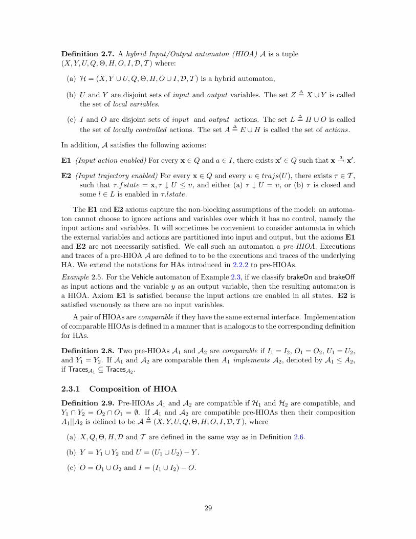
Definition 2.7. A hybrid Input/Output automaton (HIOA) A is a tuple(X,Y, U,Q,Θ,H,O, I,D, T ) where:
(a) H = (X,Y ∪ U,Q,Θ,H,O ∪ I,D, T ) is a hybrid automaton,
(b) U and Y are disjoint sets of input and output variables. The set Z ∆= X ∪ Y is calledthe set of local variables.
(c) I and O are disjoint sets of input and output actions. The set L ∆= H ∪ O is calledthe set of locally controlled actions. The set A ∆= E ∪H is called the set of actions.
In addition, A satisfies the following axioms:
E1 (Input action enabled) For every x ∈ Q and a ∈ I, there exists x′ ∈ Q such that x a→ x′.
E2 (Input trajectory enabled) For every x ∈ Q and every υ ∈ trajs(U), there exists τ ∈ T ,such that τ.fstate = x, τ ↓ U ≤ υ, and either (a) τ ↓ U = υ, or (b) τ is closed andsome l ∈ L is enabled in τ.lstate.
The E1 and E2 axioms capture the non-blocking assumptions of the model: an automa-ton cannot choose to ignore actions and variables over which it has no control, namely theinput actions and variables. It will sometimes be convenient to consider automata in whichthe external variables and actions are partitioned into input and output, but the axioms E1and E2 are not necessarily satisfied. We call such an automaton a pre-HIOA. Executionsand traces of a pre-HIOA A are defined to to be the executions and traces of the underlyingHA. We extend the notations for HAs introduced in 2.2.2 to pre-HIOAs.
Example 2.5. For the Vehicle automaton of Example 2.3, if we classify brakeOn and brakeOffas input actions and the variable y as an output variable, then the resulting automaton isa HIOA. Axiom E1 is satisfied because the input actions are enabled in all states. E2 issatisfied vacuously as there are no input variables.
A pair of HIOAs are comparable if they have the same external interface. Implementationof comparable HIOAs is defined in a manner that is analogous to the corresponding definitionfor HAs.
Definition 2.8. Two pre-HIOAs A1 and A2 are comparable if I1 = I2, O1 = O2, U1 = U2,and Y1 = Y2. If A1 and A2 are comparable then A1 implements A2, denoted by A1 ≤ A2,if TracesA1 ⊆ TracesA2 .
2.3.1 Composition of HIOA
Definition 2.9. Pre-HIOAs A1 and A2 are compatible if H1 and H2 are compatible, andY1 ∩ Y2 = O2 ∩ O1 = ∅. If A1 and A2 are compatible pre-HIOAs then their compositionA1||A2 is defined to be A ∆= (X,Y, U,Q,Θ,H,O, I,D, T ), where
(a) X,Q,Θ,H,D and T are defined in the same way as in Definition 2.6.
(b) Y = Y1 ∪ Y2 and U = (U1 ∪ U2)− Y .
(c) O = O1 ∪O2 and I = (I1 ∪ I2)−O.
29

Like hybrid automata, we would like to have a theorem that states that HIOAs areclosed under composition. However, in general the composition of two HIOAs A1 and A2
is not a HIOA. The problem arises when the the input variables of A1 are output variablesof A2 and vice-versa, such that the trajectories of these variables defined by the automataare inconsistent (see Example 6.11 in [LSV03]). As a result, the composed entity A1||A2
does not have trajectories that allow time to elapse, and therefore it does not satisfy E2.Thus, we have the following weaker theorem (from [LSV03]) which states that pre-HIOAsare closed under composition.
Theorem 2.4. If A1 and A2 are compatible hybrid I/O automata then A1||A2 is a pre-HIOA.
The next theorem is the HIOA analogue of the substitutivity Theorem 2.5.
Theorem 2.5. Suppose A1 and A2 are comparable pre-HIOAs and A1 ≤ A2. If B is apre-HIOA that is compatible with each of A1 and A2, then A1||B and A2||B are comparableand A1||B ≤ A2||B.
2.4 Structured Hybrid I/O Automata
The set of trajectories of a HA or a HIOA is described by a set of functions that satisfythe closure properties T1-3. For developing verification techniques that rely on analysis ofthe trajectories, we would like to have a structured way of specifying them. State modelsconsisting of differential and algebraic equations have served as a standard language for de-scribing the trajectories of continuous time systems (see any standard textbook in controltheory, e.g., [Oga97, Lue79]). A hybrid system may have several state models, each describ-ing the dynamics of the continuous variables under a different set of conditions. In thissection, we describe Structured Hybrid I/O Automata (SHIOA) which was first introducedin [MLL06]. An SHIOA is similar to a HIOA except that it uses a collection of state modelsfor partitioning the state space into several pieces and for describing the trajectories withineach piece by Differential and Algebraic Inequalities (DAIs).
2.4.1 State models
First, we define state models independent of any automaton, then, in Section 2.4.2, weuse state models for defining trajectories of SHIOAs. We assume that all variables areeither discrete or continuous. Suppose V is a set of variables. For a real-valued continuousvariable x ∈ V , a V-algebraic inequality is an expression of the form x ≶ f(v), where f is afunction that maps val(V ) to R and ≶ is an element of the set =,≤,≥, <,>. A trajectoryτ ∈ trajs(V ) satisfies the inequality x ≶ f(v), if
∀ t ∈ dom(τ), (τ ↓ x)(t) ≶ f(τ(t)).
A V-differential inequality for x is an expression of the form d(x) ≶ f(v), where f isa function that maps val(V ) to R. A trajectory τ ∈ trajs(V ) satisfies the differentialinequality d(x) ≶ f(v), if f τ : dom(τ) → R is an integrable function and
∀ t1, t2 ∈ dom(τ), t1 ≤ t2, (τ ↓ x)(t2)− (τ ↓ x)(t1) ≶∫ t2
t1
f(τ(s))ds.
30

A V-DAI for a set of variables Z ⊆ V is a collection of inequalities each of which is eithera V -algebraic inequality or a V -differential inequality for some variable in Z. A trajectoryτ ∈ trajs(V ) satisfies a collection F of V -DAIs for Z, if it satisfies each of the inequalitiesin F . The set of trajectories satisfying a given set of DAIs for Z may be empty.
The right hand sides of differential and algebraic inequalities are functions of the vari-ables and do not contain time explicitly. Thus, the DAIs impose time invariant constraintson how the values of the variables can change.
Lemma 2.6. Let V be a set of variables, F be a collection of V -DAIs, and τ be a trajectoryfor V that satisfies F . For any c > 0, τ + c also satisfies F .
Proof. Let x be a variable in V and x ≶ f(x) be any V -algebraic equation in F . Since τsatisfies F , for all t ∈ dom(τ), (τ ↓ x)(t) ≶ f(τ(t)). As for all t ∈ dom(τ), τ(t) = (τ+c)(t+c),it follows that ((τ + c) ↓ x)(t+ c) ≶ f((τ + c)(t+ c)). That is, τ + c satisfies all V -algebraicequations in F .
Next, suppose d(x) ≶ f(x) is any V -differential equation in F . Let us fix t1, t2 ∈dom(τ+c). We know that ((τ+c) ↓ x)(t2)−((τ+c) ↓ x)(t1) = (τ ↓ x)(t2−c)−(τ ↓ x)(t1−c).Since τ satisfies F , we obtain ((τ + c) ↓ x)(t2)− ((τ + c) ↓ x)(t1) ≶
∫ t2−ct1−c f(τ(s))ds,
≶∫ t2−c
t1−cf((τ + c)(s+ c))ds [since τ(s) = (τ + c)(s+ c) for all s].
≶∫ t2
t1
f((τ + c)(u))du [by change of variable, u = s+ c].
A state model combines a collection of DAIs with an invariant condition and a stoppingcondition. The invariant condition is used to define a subset of the state space over whichthe DAIs are active in governing continuous evolution. Each state model can be thoughtof as a mode of the hybrid system. The stopping condition, on the other hand, definesthe states at which the trajectories defined by the DAIs must stop, and this in turn forcestransitions to occur.
Definition 2.10. A state model S is a 6-tuple (X,Y, U, F, Inv, Stop), where X,Y, U aredisjoint sets of variables called internal, output, and input variables, respectively; V ∆=X ∪ Y ∪ U and Z
∆= X ∪ Y ; F is a collection of V -DAIs for the continuous variables in Z;Inv and Stop are subsets of val(X). If Inv and Stop are specified as predicates on X thenthey are called the invariant condition and the stopping condition of S.
Notations. We denote the components of a state model S by XS , YS , US , FS , InvS , andStopS , and the components of a state model Si by Xi, Yi, Ui, Fi, Invi, and Stopi.
Definition 2.11. Given a state model S = (X,Y, U, F, Inv, Stop) trajs(S) is the set oftrajectories for X ∪ Y ∪ U defined as follows: a trajectory τ is in trajs(S) if and only if:
1. The discrete variables in X remain constant over τ .
2. τ satisfies all the DAIs in F .
3. At every point in time t ∈ dom(τ), (τ ↓ X)(t) ∈ Inv.
31

4. If (τ ↓ X)(t) ∈ Stop for some t ∈ dom(τ), then τ is closed and t = τ.ltime.
Example 2.6. The trajectories for the Vehicle HA of Example 2.3 can be described by thetwo state models shown in Table 2.6. For example, a trajectory τ ∈ trajs(braking) if:
braking not braking
X x1, x2, x3, b x1, x2, x3, b
Y y y
U − −
F −amax ≤ x3 ≤ −amin x3 = 0
d(x2) = x3, d(x1) = x2 d(x2) = x3, d(x2) = x1
y = x1 y = x1
Inv b ¬b
Stop f alse f alse
Table 2.1: State models specifying trajectories of Vehicle.
(i) For all t ∈ dom(τ)
1. (τ ↓ b)(t) = true,
2. (τ ↓ x1)(t) = (τ ↓ y)(t), and
3. −amax ≤ (τ ↓ x3)(t) ≤ −amin.
(ii) τ ↓ x3 : dom(τ) → R is an integrable function.
(iii) For all t1, t2 ∈ dom(τ) and i ∈ 1, 2, (τ ↓ xi)(t2)− (τ ↓ xi)(t1) =∫ t2t1
(τ ↓ xi+1)(s)ds.
Associating an invariant set with each set F of DAIs allow us to avoid parts of thestate space, for example singularities, where the equations in F may not be well formed.The stopping conditions provide a mechanism to define trajectories which satisfy certainconditions at all points in time, except possibly at the right end-point. Suppose we wishto model the positions of two vehicles represented by variables x and y. The vehicles movealong a single track according to the DAIs F1 until they collide. After a collision occurs,their dynamics is specified by DAIs F2. Now, if we associate x 6= y as an invariant for thefirst state model S1 then trajs(S1) will not contain the trajectories which lead to collisions.However, if we associate x = y as a stopping condition for S1 then trajs(S1) may containtrajectories which satisfy x = y at their right endpoint.
In order to capture that F2 (and not F1) describes the dynamics after a collision, fol-lowing the modeling style of [DL97], we add an action that is enabled when x = y and thatit sets a boolean variable collided to true. Then we add collided and ¬collided as invariantconditions for S2 and S1, respectively.
Next, we show that the sets of trajectories specified by state models satisfy T1, T2,and T3.
Proposition 2.7. Consider a state model S.
32

(i) If τ ∈ trajs(S) then any prefix and any suffix of τ is also in trajs(S).
(ii) If τ0, τ1 ∈ trajs(S), τ0 is closed and τ0.lval d X = τ1.fval d X, then τ0_τ1 ∈ trajs(S).
Proof. Let S = (X,Y, U, F, Inv, Stop) and τ1 be a trajectory in trajs(S). For Part (i),it is routine to check that any prefix (and suffix) of τ1 satisfies all the four conditions inDefinition 2.11, and therefore is also in the set trajs(S).
For Part(ii), we show that τ2∆= τ0
_ τ1 is in traj(S) by checking that it satisfies the fourconditions in Definition 2.11.
1. Let x be a discrete variable in X. From Part 1 of Definition 2.11 we know that xremains constant over τ0 and τ1. Since τ0.lval d X = τ1.fval d X, it follows that xremains constant over τ2.
2. Let x be a continuous variable in X ∪ Y and f be a function over the values of thevariables in X ∪ Y ∪ U . Since τ0 and τ1 satisfy every algebraic inequality in F , ofthe form x ≶ f(v), so does τ2. To show that τ2 satisfies any differential inequalityof the form d(x) ≶ f(v) in F , consider t0, t1 ∈ dom(τ2), t1 ≥ t0. The interestingcase arises when t0 < τ0.ltime and t1 > τ0.ltime. Let t2 = τ0.ltime. We can write(τ2 ↓ x)(t1)− (τ2 ↓ x)(t0) as
(τ2 ↓ x)(t1)− (τ2 ↓ x)(t2) + (τ2 ↓ x)(t2)− (τ2 ↓ x)(t0)= ((τ1 + t2) ↓ x)(t1)− ((τ1 + t2) ↓ x)(t2) + (τ0 ↓ x)(t2)− (τ0 ↓ x)(t0)
≶∫ t1
t2
f((τ1 + t2)(s))ds+∫ t2
t0
f(τ0(s))ds
≶∫ t1
t2
f(τ2(s))ds+∫ t2
t0
f(τ2(s))ds =∫ t1
t0
f(τ2(s))ds.
In rewriting the second expression we have used the fact that τ0 and τ1 + t2 satisfythe differential inequality d(x) ≶ f(v)—the latter follows from Lemma 2.6. The laststep follows from the fact that, for all s ∈ [t2, t1], (τ1 + t2)(s) = τ2(s).
3. Immediate from definition of τ2.
4. We consider two cases here. If τ0.lval d X ∈ Stop, then τ1.fval d X ∈ Stop and τ1is a point trajectory, that is, τ2 = τ0. Otherwise, from Part 4 of Definition 2.11 itfollows that for every t ∈ dom(τ2) except possibly τ1.ltime, τ2(t) d X /∈ Stop.
2.4.2 Definition of Structured HIOA
A Structured Hybrid I/O Automaton (SHIOA) is a state machine model that uses a collec-tion of state models for specifying its trajectories.
Definition 2.12. A Structured Hybrid I/O Automaton (SHIOA) A is a tuple(X,Y, U,Q,Θ,H,O, I,D,S ) where
(a) X,Y and U are disjoint sets of internal, output and input variables. The set V ∆=X ∪ Y ∪ U is the set of variables, and Z ∆= X ∪ Y is the set of local variables.
33

(b) A set Q ⊆ val(X) of states and a non-empty subset Θ ⊆ Q of start states.
(c) H,O and I are disjoint sets of internal, output and input actions. The set A ∆=H ∪ I ∪O is the set of actions, and L ∆= H ∪O is the set of local actions.
(d) A set D ⊆ Q×A×Q of discrete transitions.
(e) A collection S of state models such that for each state model S ∈ S , XS = X,YS = Y , and US = U , and for every pair S,S ′ ∈ S , InvS ∩ InvS′ = ∅.
In addition, A satisfies the following axioms:
E1 (Input action enabled) For every input action a ∈ I and for every state x ∈ Q, thereexists a state x′ ∈ Q such that x a→ x′.
S1 (Complete) Q ⊆⋃S∈S InvS .
S2 (Input trajectory enabled) For every trajectory υ ∈ trajs(U) of the input variables,for every state model S ∈ S and every state x ∈ InvS , there exists a trajectoryτ ∈ trajs(S) with τ.fstate = x, τ ↓ U ≤ υ, and either (a) τ ↓ U = υ, or (b) τ isclosed and some local action in L is enabled at τ.lstate.
E1 is the same action nonblocking axiom as in the the case of HIOAs. The S1 axiomensures that the disjoint invariant sets of the state models together cover the state spaceQ. Axiom S2 is a non-blocking axiom for individual state models: given any trajectory υof the input variables and any state model, either time can elapse for the entire duration ofυ, or time elapses to a point at which some local action of A is enabled. An SHIOA whichdoes not necessarily satisfy S2 is called a pre-SHIOA.Notations. We denote the components of a pre-SHIOA A by XA, YA, UA, QA,SA etc.,and the components of an pre-SHIOA Ai by Xi, Yi, Ui, Qi,Si, etc. Given a pre-SHIOAA we define HIOA(A) to be the structure (XA, YA, UA, QA,ΘA,HA, OA, IA,DA, T ), whereT =
⋃S∈SA
trajs(S). Note that HIOA(A) may not necessarily be a HIOA. The next tworesults state that by augmenting the variables, actions, and discrete transitions with a setof state models, what we obtain is either a HIOA or a pre-HIOA depending on whether onnot the state models satisfy axioms S1 and S2.
Lemma 2.8. If A is a pre-SHIOA then HIOA(A) is a pre-HIOA.
Proof. From Proposition 2.7 we know that for each state model S of A, trajs(S) satisfiesaxioms T1, T2, and T3 of Definition 2.3. Therefore, the set T of trajectories of HIOA(A),defined as
⋃S∈SA
trajs(S) satisfies T1 and T2. Consider τ1, τ2 ∈ T , such that τ1 is closedand τ1.lval d X = τ2.fval d X. Suppose τ1 ∈ trajs(S) for some state model S of A.Then τ1.lstate ∈ InvS and as τ1.lstate = τ2.fstate, τ2.fstate ∈ InvS . Since the invariantconditions for the state models of A are disjoint, it follows that τ2 ∈ trajs(S), and thereforeτ1
_ τ2 ∈ trajs(S) ⊆ T . Thus, T also satisfies T3. Since A satisfies axiom E1 and the setsof discrete transitions of A and HIOA(A) are identical, HIOA(A) also satisfies E1.
Theorem 2.9. If A is an SHIOA then HIOA(A) is a HIOA.
34
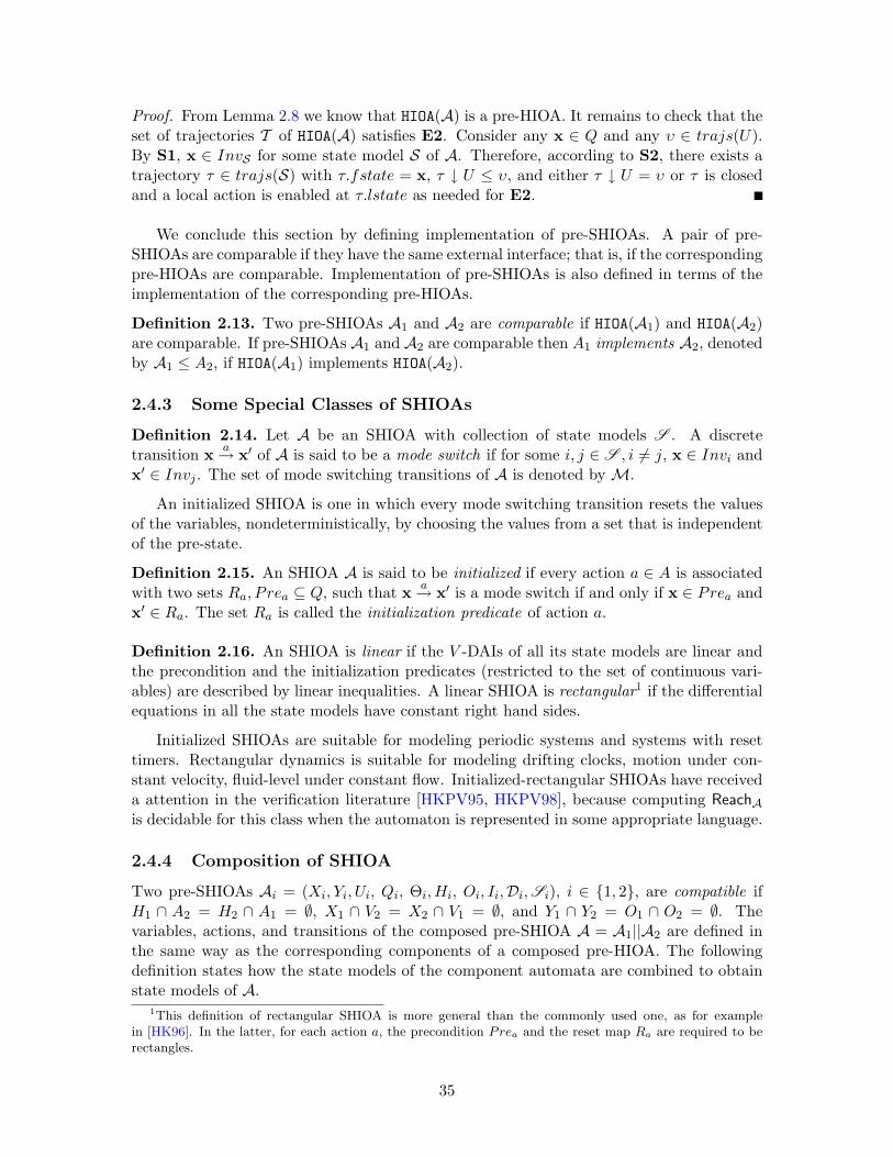
Proof. From Lemma 2.8 we know that HIOA(A) is a pre-HIOA. It remains to check that theset of trajectories T of HIOA(A) satisfies E2. Consider any x ∈ Q and any υ ∈ trajs(U).By S1, x ∈ InvS for some state model S of A. Therefore, according to S2, there exists atrajectory τ ∈ trajs(S) with τ.fstate = x, τ ↓ U ≤ υ, and either τ ↓ U = υ or τ is closedand a local action is enabled at τ.lstate as needed for E2.
We conclude this section by defining implementation of pre-SHIOAs. A pair of pre-SHIOAs are comparable if they have the same external interface; that is, if the correspondingpre-HIOAs are comparable. Implementation of pre-SHIOAs is also defined in terms of theimplementation of the corresponding pre-HIOAs.
Definition 2.13. Two pre-SHIOAs A1 and A2 are comparable if HIOA(A1) and HIOA(A2)are comparable. If pre-SHIOAs A1 and A2 are comparable then A1 implements A2, denotedby A1 ≤ A2, if HIOA(A1) implements HIOA(A2).
2.4.3 Some Special Classes of SHIOAs
Definition 2.14. Let A be an SHIOA with collection of state models S . A discretetransition x a→ x′ of A is said to be a mode switch if for some i, j ∈ S , i 6= j, x ∈ Invi andx′ ∈ Invj . The set of mode switching transitions of A is denoted by M.
An initialized SHIOA is one in which every mode switching transition resets the valuesof the variables, nondeterministically, by choosing the values from a set that is independentof the pre-state.
Definition 2.15. An SHIOA A is said to be initialized if every action a ∈ A is associatedwith two sets Ra, P rea ⊆ Q, such that x a→ x′ is a mode switch if and only if x ∈ Prea andx′ ∈ Ra. The set Ra is called the initialization predicate of action a.
Definition 2.16. An SHIOA is linear if the V -DAIs of all its state models are linear andthe precondition and the initialization predicates (restricted to the set of continuous vari-ables) are described by linear inequalities. A linear SHIOA is rectangular1 if the differentialequations in all the state models have constant right hand sides.
Initialized SHIOAs are suitable for modeling periodic systems and systems with resettimers. Rectangular dynamics is suitable for modeling drifting clocks, motion under con-stant velocity, fluid-level under constant flow. Initialized-rectangular SHIOAs have receiveda attention in the verification literature [HKPV95, HKPV98], because computing ReachAis decidable for this class when the automaton is represented in some appropriate language.
2.4.4 Composition of SHIOA
Two pre-SHIOAs Ai = (Xi, Yi, Ui, Qi, Θi,Hi, Oi, Ii,Di,Si), i ∈ 1, 2, are compatible ifH1 ∩ A2 = H2 ∩ A1 = ∅, X1 ∩ V2 = X2 ∩ V1 = ∅, and Y1 ∩ Y2 = O1 ∩ O2 = ∅. Thevariables, actions, and transitions of the composed pre-SHIOA A = A1||A2 are defined inthe same way as the corresponding components of a composed pre-HIOA. The followingdefinition states how the state models of the component automata are combined to obtainstate models of A.
1This definition of rectangular SHIOA is more general than the commonly used one, as for examplein [HK96]. In the latter, for each action a, the precondition Prea and the reset map Ra are required to berectangles.
35

Definition 2.17. If A1 and A2 are compatible pre-SHIOAs then their composition A1||A2
is (X,Y, U,Q,Θ,H,O, I,D,S ) where
1. The sets X,Y, U,Q,Θ,H,O, I, and D are defined as in Definition 2.9.
2. Suppose the state models in S1 and S2 are indexed by sets I1 and I2. For each i ∈ I1and j ∈ I2, the combination of (X1, Y1, U1, Fi, Invi, Stopi) ∈ S1 and (X2, Y2, U2, Fj ,Invj , Stopj) ∈ S2 is the state model Sij = (X,Y, U, F, Inv, Stop), where
F is the collection of all DAIs in Fi and Fj ,
Inv = x ∈ val(X) | x d X1 ∈ Invi ∧ x d X2 ∈ Invj, and
Stop = x ∈ val(X) | x d X1 ∈ Stopi ∨ x d X2 ∈ Stopj.
The set of state models S for A1||A2 is the collection Sij.
For the reasons described in Section 2.3.1, the class of SHIOAs is not closed undercomposition, but the class of pre-SHIOAs is:
Theorem 2.10. If A1 and A2 are compatible pre-SHIOAs then A = A1||A2 is a pre-SHIOA.
Proof. Let Ai = (Xi, Yi, Ui, Qi,Θi,Hi, Oi, Ii,Di,Si), for i ∈ 1, 2. Since the variables,actions, and transitions of A are defined according to Definition 2.9, A satisfies E1. Thus,it suffices to check that SA is a collection of state models for A, with disjoint invariant setsand that SA satisfies the completeness condition S1.
Let us fix a state model Si = (X1, Y1, U1, Fi, Invi, Stopi) from S1 and another statemodel Sj = (X2, Y2, U2, Fj , Invj , Stopj) from S2, and investigate their combination Sij =(X,Y, U, F ′, Inv′, Stop′). Fi and Fj are collections of DAIs for the continuous variablesin X1 ∪ Y1 and X2 ∪ Y2, respectively. Therefore, F is a collection of DAIs for the set ofcontinuous variables in X1 ∪ Y1 ∪X2 ∪ Y2, which by Definition 2.17 is the same as the setof continuous variables in ZA.
Consider a different state model Skl of A obtained by combining Sk ∈ S1 with Sl ∈ S2.Since Sij is different from Skl, we assume without loss of generality that j 6= l. For anyx ∈ InvSij , by Definition 2.17, x d X2 ∈ Invj . Since Invj ∩ Invl = ∅, x d X2 /∈ Invl, andtherefore x /∈ InvSkl
. Thus, any two state models of A have disjoint invariant sets.For the completeness condition, consider a state x ∈ QA. Since x d X1 ∈ Q1, from
the completeness of S1 we know that there exists Si ∈ S1, such that x d X1 ∈ Inv(Si).Likewise, from completeness of S2, there exists Sj ∈ S2, such that x d X2 ∈ Inv(Sj). Itfollows that for any x ∈ QA, x ∈ Inv(Sij) ⊆
⋃S∈SA
Inv(S).
Although we shall use pre-SHIOAs for systematically describing the trajectories of hy-brid systems, the underlying objects are really HIOAs and pre-HIOAs. We show that theoperator HIOA and the composition operation interact in the expected way. Formally, HIOAis a homomorphism from the set of pre-SHIOAs to the set of pre-HIOAs, which preservesthe composition operation within each of these sets.
Theorem 2.11. If A1 and A2 are compatible pre-SHIOAs then HIOA(A1)||HIOA(A2) =HIOA(A1||A2).
36

Proof. Let T be the set of trajectories of HIOA(A1)||HIOA(A2) and T ′ be the set of trajec-tories for HIOA(A1||A2). It suffices to show that T = T ′. Let S be the collection of statemodels for the composed pre-SHIOA A1||A2; that is, T ′ ∆=
⋃S∈S trajs(S).
First, we show that T ⊆ T ′. Consider a trajectory τ ∈ T . From Definition 2.9 weknow that τ ↓ V1 is in T1, where T1 =
⋃S∈S1
trajs(S) is the set of trajectories of HIOA(A1).That is, there exists S1 ∈ S1, such that T1 ↓ V1 ∈ trajs(S1). Likewise, τ ↓ V2 ∈ T2 =⋃S∈S2
trajs(S) and there exists S2 ∈ S2, such that T2 ↓ V2 ∈ trajs(S2). Then, τ ∈trajs(S12), where S12 is the state model for the composed pre-SHIOA A1||A2 obtained bycombining S1 and S2. Thus, τ ∈ trajs(S12) ⊆ T ′.
Next, we show that T ′ ⊆ T . Consider a trajectory τ ∈ T ′ =⋃S∈S trajs(S). There
exists Sij ∈ S , such that τ ∈ trajs(Sij), where Sij ∈ S obtained by combining someSi ∈ S1 and Sj ∈ S2. Thus, τ ↓ V1 ∈ trajs(Si) ⊆ T1 and τ ↓ V2 ∈ trajs(Sj) ⊆ T2, and itfollows that τ is in T .
Corollary 2.12. If A1 and A2 are compatible SHIOAs and their composition A1||A2 is anSHIOA, then HIOA(A1)||HIOA(A2) is a HIOA.
Proof. From Theorem 2.11 we know HIOA(A1||A2) = HIOA(A1)||HIOA(A2). Since A1||A2 isan SHIOA, from Theorem 2.9 it follows that HIOA(A1||A2) and therefore HIOA(A1)||HIOA(A2),is also a HIOA.
2.4.5 Summary
We presented the basic definitions and results that underlie the Structured Hybrid I/OAutomaton (SHIOA) framework. Much the the foundational concepts came from the HybridI/O Automaton (HIOA) framework of [LSV03]. The SHIOA incorporate state models inthe HIOA framework for the purpose of systematically describing trajectories. The idea ofstate models, as in SHIOAs, is related to the similar notion of state-space description ofcontinuous time systems. However, in addition to the differential and algebraic equationsthat describe the evolution of the variables in such state-space models, the state modelsmay also contain invariants and stopping conditions. These additional features capture theessence of hybrid systems where discrete transitions bring changes in the state variablesthat in turn change the state model that govern further evolution. In the next chapter wedevelop the HIOA language for specifying SHIOAs; the design of this language relies heavilyon the state model structure. In Chapters 4, 5, and 6 we develop tools and techniques forverifying SHIOAs; these are also aided by the state model structure.
37
Chapter 3
The HIOA Language
HIOA is a language for succinctly and precisely specifying hybrid systems. The semantics ofthe language is based on the Structured Hybrid I/O Automata (SHIOA) model introducedin Chapter 2. This language is used throughout Part I for describing hybrid systems. TheHIOA language evolved in part from the IOA language [GLTV03] which has been widelyused for specifying untimed distributed systems. The new features of the HIOA language,namely the constructs for continuous variables and trajectories, are based on the workpresented in [MWLF03, Mit01, KLMG05]. A somewhat restricted version of HIOA, whichdoes not allow external variables, is implemented as part of the Tempo Toolkit [TEM07].In Chapter 6 we will show how HIOA specifications can be translated to the language ofthe PVS Theorem prover [ORR+96]. In Section 7.7 of Part II, HIOA is extended to allowspecification of probabilistic transitions. In this Chapter, we describe the key features ofthe language through a sequence of small examples.
3.1 An Overview
Consider a SHIOA Bounce describing the position and the velocity of a ball bouncing on asurface. The HIOA language specification for Bounce is shown in Figure 3-1. The first lineconsists of the keyword automaton followed by the automaton’s name Bounce, and a listof formal parameters. Formal parameters are used for succinctly specifying sets of objectssuch as automata, actions, trajectories, etc. In this example, the coefficient of restitution ρof the surface is a real-valued formal parameter of Bounce. The value of ρ is restricted to bestrictly between 0 and 1 using a where-clause. Where-clauses are predicates that constrainvalues of formal parameters and therefore are useful for avoiding ill-formed specifications,such as those resulting from division-by-zero. Usage of formal parameters and where-clausesare further described in Section 3.2.4.
The body of the specification of Bounce has four sections: (a) signature, (b) variables,(c) transitions, and (d) trajectories. The signature section declares the names and kindsof actions of the automaton. Bounce has a single output action called bounce. The otherkinds of actions that an automaton can have are input and internal. Signature definitionsare discussed in further detail in Section 3.4.
The variables of an automaton are declared by the keyword variables followed by listof variables, their kinds, types, dynamic types, and possibly their initial values. Bouncehas a real-valued internal variable v with initial value 0, and a real-valued output variablex with initial value 100. In HIOA all real valued variables are implicitly continuous. In
38
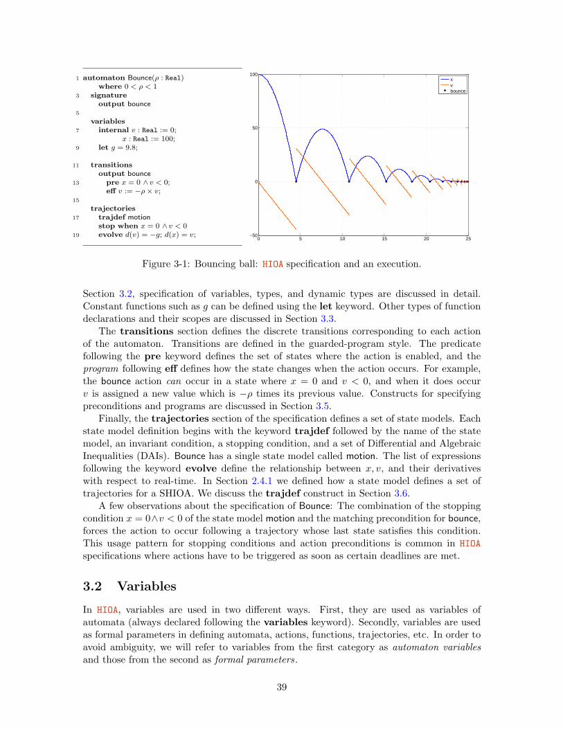
1 automaton Bounce(ρ : Real)where 0 < ρ < 1
3 signatureoutput bounce
5
variables7 internal v : Real := 0;
x : Real := 100;9 let g = 9.8;
11 transitionsoutput bounce
13 pre x = 0 ∧ v < 0;eff v := −ρ× v;
15
trajectories17 trajdef motion
stop when x = 0 ∧ v < 019 evolve d(v) = −g; d(x) = v;
0 5 10 15 20 25−50
0
50
100
xvbounce
Figure 3-1: Bouncing ball: HIOA specification and an execution.
Section 3.2, specification of variables, types, and dynamic types are discussed in detail.Constant functions such as g can be defined using the let keyword. Other types of functiondeclarations and their scopes are discussed in Section 3.3.
The transitions section defines the discrete transitions corresponding to each actionof the automaton. Transitions are defined in the guarded-program style. The predicatefollowing the pre keyword defines the set of states where the action is enabled, and theprogram following eff defines how the state changes when the action occurs. For example,the bounce action can occur in a state where x = 0 and v < 0, and when it does occurv is assigned a new value which is −ρ times its previous value. Constructs for specifyingpreconditions and programs are discussed in Section 3.5.
Finally, the trajectories section of the specification defines a set of state models. Eachstate model definition begins with the keyword trajdef followed by the name of the statemodel, an invariant condition, a stopping condition, and a set of Differential and AlgebraicInequalities (DAIs). Bounce has a single state model called motion. The list of expressionsfollowing the keyword evolve define the relationship between x, v, and their derivativeswith respect to real-time. In Section 2.4.1 we defined how a state model defines a set oftrajectories for a SHIOA. We discuss the trajdef construct in Section 3.6.
A few observations about the specification of Bounce: The combination of the stoppingcondition x = 0∧v < 0 of the state model motion and the matching precondition for bounce,forces the action to occur following a trajectory whose last state satisfies this condition.This usage pattern for stopping conditions and action preconditions is common in HIOAspecifications where actions have to be triggered as soon as certain deadlines are met.
3.2 Variables
In HIOA, variables are used in two different ways. First, they are used as variables ofautomata (always declared following the variables keyword). Secondly, variables are usedas formal parameters in defining automata, actions, functions, trajectories, etc. In order toavoid ambiguity, we will refer to variables from the first category as automaton variablesand those from the second as formal parameters.
39

Each automaton variable is of one of three kinds, namely, input, output, or internal.The kind of a variable is specified by the corresponding keyword preceding its name.
3.2.1 Built-in Types
All variables are associated with types. There are several built-in types, such as, Bool, Char,Int, Nat, Real, AugmentedReal, and String that do not require explicit definitions. TheAugmentedReal type is Real∪∞,−∞. In modeling embedded systems as SHIOAs, oftenwe have to define a real-time upper-bound within which an action has to occur. As theautomaton executes, this upper-bound may change. A common idiom in HIOA is to modelsuch bounds by the value of a deadline variable (see, Example 3.4). AugmentedReal is auseful type for such a deadline variable because setting the variable to ∞ implies that itdoes not impose any deadline.
Additional types can be defined using the following type constructors: Enumeration [e1, e2, e3]: finite set with elements e1, e2, and e3. Null [E]: E extended by a single element nil. Tuple [I1 : E1, . . . In : En]: n-tuple with fields I1, . . . , In of types, E1, . . . En. Union [I1 : E1, . . . In : En]: union of types E1, . . . En with accessors I1, . . . , In. Seq [E]: finite sequence of elements of type E. Set [E]: finite set of elements of type E. Mset [E]: finite multiset of elements of type E. Map [D1, . . . , Dn, E]: finite (possibly partial) mapping of D1 × . . .×Dn to E. Array [I1, . . . , In, E]: n-dimensional array of type E indexed by element of types
I1, . . . , In where the indices are of finite types.Type constructors can be nested and can be used in-place to declare types of formal andautomaton variables. For example, the code fragment
variablesinternal buffer: Seq [Bool],output position: Tuple [x : Real, y : Real, z : Real]
defines an internal variable buffer which takes values in 0, 1∗, and an output variableposition which takes values in R3. A restricted version of the HIOA language, which does notallow input/output variables, is called the TIOA language. Current implementation of theTIOA language is available as a part of the Tempo toolset [TEM07] In this implementation,type equivalences are decided based on types names, and hence, two types with identicaldefinitions but with different names are judged to be distinct.
3.2.2 Vocabularies
Named types are defined using the vocabularies construct. Vocabularies can define con-crete as well as uninterpreted types, and also operators on these types. The HIOA languageallows polymorphic types and operators, using which one can specify automata that ma-nipulate objects of polymorphic types.
In Figure 3-2 a vocabulary for directed graphs is defined and used in the updateGraphautomaton. Vocabulary definitions consist of the keyword vocabulary, followed by thename of the vocabulary, followed by an optional list of formal parameters. The vocabularydirectedGraphs has a single formal type parameter T . Type parameters are special kindsof formal parameters which denote a type. They are declared using the keyword typeand they provide a mechanism for polymorphic HIOA specifications. In this example, the
40

type parameter T specifies the type of the vertices of the directed graphs defined by thedirectedGraphs vocabulary. The main body of any vocabulary definition has two sections:(a) types and (b) operators. The types section introduces names and definitions for types.The directedGraphs vocabulary introduces the types Edge,Digraph, and Path. The typeEdge is defined as an ordered pair of elements of type T . Digraph is defined as an orderedpair of sets—the first component vset is a set of type T and the second component eset isa set of Edges. The type Path is defined as a finite sequence of elements of type T . Theoperators section introduces a set of operator names and their signatures. For example,directedGraphs has two operators connected and addEdge. The connected operator takesa pair of elements of type T and returns a boolean. The addEdge operator takes a Digraphand an Edge and returns a Digraph.
If directedGraphs(Nat) is imported into an automaton, then all the type and operatordefinitions in directedGraphs are interpreted with T replaced by Nat. For example, theinitial graph G would be an arbitrary graph with a set of natural numbers as vertices. Theautomaton updateGraph of Figure 3-2 imports directedGraphs(V ), where V is a formaltype parameter of the automaton. This illustrates how we can specify an automaton thatperforms operations on generic graphs without ever instantiating the type of the graphvertices.
Of course, for proving or model-checking properties of the automaton, for simulatingit, or for generating executable code from the HIOA specification, it may become necessaryto assert additional properties or to provide implementations of the types and operations.For example, these may take the form of axioms stating key properties of the connectedfunction for a theorem prover, or a Java implementation of the Digraph data-type fora code generator. These are provided as appropriate auxiliary files to the back-end toolsindependent of the HIOA language. In Chapter 6 we discuss this in more detail in the contextof the PVS theorem prover.
1 vocabulary directedGraphs(T :type)types
3 Edge = Tuple [src : T, dst : T ];Digraph =
5 Tuple [vset :Set[T ], eset :Set[Edge]];Path = Seq [T ];
7
operators9 connected : T, T → Bool;
addEdge : Digraph,Edge→ Digraph;11 end
12
automaton updateGraph(V : type)14imports directedGraphs(V )
16signatureinput add(e : Edge)
18
variables20internal G : Digraph;
22transitionsinput add(e)
24eff G := addEdge(G, e);
Figure 3-2: Vocabulary for graphs.
3.2.3 Dynamic Types
All automaton variables are associated with dynamic types. In HIOA, dynamic types canbe either discrete or continuous (see, Definition 2.2). The dynamic type of a variable isdeclared implicitly; it is inferred automatically from the variable’s static type. For variablesof all built-in simple types except Real the dynamic type is discrete. The dynamic type ofReal variables is continuous. For defining a Real variable with discrete dynamic type, itstype name is qualified with the keyword Discrete.
41

If the type of a variable v is defined by one of the type constructors Tuple or Array,then dtype(v) is defined as follows. The variable v is viewed as a ordered tuple of variablesv1, . . . , vk, for some finite k. The type of v, type(v) = type(v1) × . . . × type(vk). Thedynamic type of v is the set of functions f from left-closed intervals of time to type(v) suchthat f.vi ∈ dtype(vi) for each i ∈ 1, . . . , k.
If the type of v is defined by nesting the type constructors Tuple and Array, then thedtype(v) is defined recursively using the above rule. The dynamic type of all other compoundtypes and user-defined types is discrete. Consider the following vocabulary definition:
vocabulary matrixtypesT : Tuple [a : Real, b : Nat, c : Discrete Real],Row: Enumeration [p1, p2, p3],Col: Enumeration [q1, q2, q3],matrix: Array [Row,Col, Real],intMatrix: Array [Row,Col, Int]
end
Suppose that variable v is declared to be of type T . Then dtype(v) is the set of functionsf from left-closed intervals of time to T such that f.a is piecewise continuous with realvalues, f.b is piecewise constant with natural values, and f.c is piecewise constant with realvalues. The type matrix represents a 3 × 3 array of real numbers. A variable x declaredto be of type matrix can be viewed as an ordered 9-tuple of reals. The dynamic type of xis the set of functions f from left-closed intervals of time to R9 such that the restriction off on each of the coordinates is a piecewise continuous function from left-closed intervals oftime to R. A variable y of type intMatrix can be viewed as an ordered 9-tuple of integers.And dtype(y) is the set of functions f from left-closed intervals of time to Z9 such that therestriction of f on each coordinate is piece-wise constant.
3.2.4 Initial Values
Initial valuations of the internal variables of an automaton may be specified in the HIOAlanguage in two ways. First, each variable can be individually initialized using the as-signment operator := followed by an expression or a nondeterministic choice over a set.The expression should not refer to any other automaton variable. This method is usedin lines 7–8 of the Bounce automaton of Figure 3-1. A nondeterministic choice is specifiedby the keyword choose followed by a set, written as a where-clause. The second method isto use the initially keyword followed by a predicate on the internal variables defining theset of allowed initial values. This selects an arbitrary value for the variables from the set ofvalues that satisfy the predicate. It is possible to mix these methods.
variablesoutput u : Discrete Real
internal x : Real := 5,y : Real := choose k where −5 ≤ k ≤ 5,z : Realinitially z × z + y × y ≤ 10
. . .
In the above code fragment, the initial value of x is set to 5, y gets some value in [−5, 5],and z is chosen such that z2 + y2 ≤ 10.
42
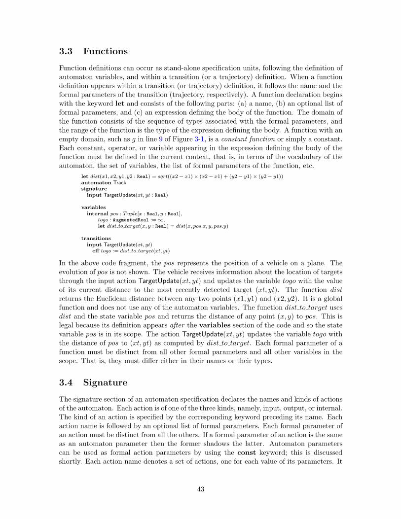
3.3 Functions
Function definitions can occur as stand-alone specification units, following the definition ofautomaton variables, and within a transition (or a trajectory) definition. When a functiondefinition appears within a transition (or trajectory) definition, it follows the name and theformal parameters of the transition (trajectory, respectively). A function declaration beginswith the keyword let and consists of the following parts: (a) a name, (b) an optional list offormal parameters, and (c) an expression defining the body of the function. The domain ofthe function consists of the sequence of types associated with the formal parameters, andthe range of the function is the type of the expression defining the body. A function with anempty domain, such as g in line 9 of Figure 3-1, is a constant function or simply a constant.Each constant, operator, or variable appearing in the expression defining the body of thefunction must be defined in the current context, that is, in terms of the vocabulary of theautomaton, the set of variables, the list of formal parameters of the function, etc.
let dist(x1, x2, y1, y2 : Real) = sqrt((x2− x1)× (x2− x1) + (y2− y1)× (y2− y1))automaton Tracksignature
input TargetUpdate(xt, yt : Real)
variablesinternal pos : Tuple[x : Real, y : Real],
togo : AugmentedReal := ∞,let dist to target(x, y : Real) = dist(x, pos.x, y, pos.y)
transitionsinput TargetUpdate(xt, yt)
eff togo := dist to target(xt, yt)
In the above code fragment, the pos represents the position of a vehicle on a plane. Theevolution of pos is not shown. The vehicle receives information about the location of targetsthrough the input action TargetUpdate(xt, yt) and updates the variable togo with the valueof its current distance to the most recently detected target (xt, yt). The function distreturns the Euclidean distance between any two points (x1, y1) and (x2, y2). It is a globalfunction and does not use any of the automaton variables. The function dist to target usesdist and the state variable pos and returns the distance of any point (x, y) to pos. This islegal because its definition appears after the variables section of the code and so the statevariable pos is in its scope. The action TargetUpdate(xt, yt) updates the variable togo withthe distance of pos to (xt, yt) as computed by dist to target. Each formal parameter of afunction must be distinct from all other formal parameters and all other variables in thescope. That is, they must differ either in their names or their types.
3.4 Signature
The signature section of an automaton specification declares the names and kinds of actionsof the automaton. Each action is of one of the three kinds, namely, input, output, or internal.The kind of an action is specified by the corresponding keyword preceding its name. Eachaction name is followed by an optional list of formal parameters. Each formal parameter ofan action must be distinct from all the others. If a formal parameter of an action is the sameas an automaton parameter then the former shadows the latter. Automaton parameterscan be used as formal action parameters by using the const keyword; this is discussedshortly. Each action name denotes a set of actions, one for each value of its parameters. It
43
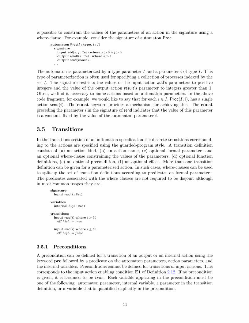
is possible to constrain the values of the parameters of an action in the signature using awhere-clause. For example, consider the signature of automaton Proc.
automaton Proc(I : type, i : I)signature
input add(k, j : Int) where k > 0 ∧ j > 0output result(k : Int) where k > 1output send(const i)
. . .
The automaton is parameterized by a type parameter I and a parameter i of type I. Thistype of parameterization is often used for specifying a collection of processes indexed by theset I. The signature restricts the values of the input action add’s parameters to positiveintegers and the value of the output action result’s parameter to integers greater than 1.Often, we find it necessary to name actions based on automaton parameters. In the abovecode fragment, for example, we would like to say that for each i ∈ I, Proc(I, i), has a singleaction send(i). The const keyword provides a mechanism for achieving this. The constpreceding the parameter i in the signature of send indicates that the value of this parameteris a constant fixed by the value of the automaton parameter i.
3.5 Transitions
In the transitions section of an automaton specification the discrete transitions correspond-ing to the actions are specified using the guarded-program style. A transition definitionconsists of (a) an action kind, (b) an action name, (c) optional formal parameters andan optional where-clause constraining the values of the parameters, (d) optional functiondefinitions, (e) an optional precondition, (f) an optional effect. More than one transitiondefinition can be given for a parameterized action. In such cases, where-clauses can be usedto split-up the set of transition definitions according to predicates on formal parameters.The predicates associated with the where clauses are not required to be disjoint althoughin most common usages they are.
signatureinput read(i : Nat)
variablesinternal high : Bool
transitionsinput read(i) where i > 50
eff high := true
input read(i) where i ≤ 50eff high := f alse
3.5.1 Preconditions
A precondition can be defined for a transition of an output or an internal action using thekeyword pre followed by a predicate on the automaton parameters, action parameters, andthe internal variables. Preconditions cannot be defined for transitions of input actions. Thiscorresponds to the input action enabling condition E1 of Definition 2.12. If no preconditionis given, it is assumed to be true. Each variable appearing in the precondition must beone of the following: automaton parameter, internal variable, a parameter in the transitiondefinition, or a variable that is quantified explicitly in the precondition.
44

3.5.2 Effects
The effect of a transition is defined in terms of a (possibly nondeterministic) programfollowing the keyword eff. The program assigns values to the internal variables of theautomaton, thus defining the post-state (i.e., the state after the transition occurs) in termsof the values of the variables in the pre-state (i.e., the state before the transition occurs).If the effect of a transition is omitted, then the state remains unchanged. The programused to specify the relation between the pre-state and the post-state of a transition is a listof statements, separated by semicolons. The statements are executed sequentially and thecomputation of the whole program is completed in a single atomic step. There are threetypes of statements: (i) assignments, (ii) conditionals, and (iii) loops, which we describenext.
Assignments
An assignment statement consists of an internal variable of the automaton followed bythe assignment operator := and either an expression (see, e.g., line 24 of Figure 3-2) or anondeterministic choice (as in the case of nondeterministic choice of initial values). Theexpression or nondeterministic choice in an assignment statement must have the same typeas the internal variable. The execution of an assignment does not have side-effects, that is,it does not change the value of any variable other than the internal variable appearing onthe left side of the assignment operator.
Conditionals
A conditional statement is used to control the flow of program execution within the effectspart of a transition. It starts with the if keyword followed by a predicate, the keywordthen, and a program segment; it ends with a keyword fi. In between there can be anynumber of elseif clauses. For example, the conditional statement
if clock ≥ Delta then timeout := true fi
assigns a value to the timeout variable based on the value of clock.
Loops
A loop is used to repeatedly execute a program segment a finite number of times—once foreach value of a variable that satisfies a given condition. A loop starts with the keywordfor followed by a variable, a predicate defining a finite set of values for this variable, and aprogram segment enclosed within the keywords do and od. For example, the for-loop
for i : Nat in S do time stamp[i] := clock od
sets the value of time stamp[i] to clock for each natural number i in the set S.
3.6 Trajectories
The trajectories section of a HIOA specification defines a set of state models for the automa-ton. These state models in turn define a set of trajectories according to Definition 2.11. Eachtrajectory definition starts with the keyword trajdef and has the following components:(a) a name for the state model, (b) optional list of formal parameters and a where-clauseconstraining the values of the parameters, (c) optional function definitions, (d) an optional
45

invariant condition, (e) an optional stopping condition, and (f) a collection of Differentialand Algebraic Inequalities (DAIs). As in the case of transition definitions, names of trajec-tory definitions can be parameterized by formal variables and the values of these parameterscan be constrained by where-clauses. In the following example, the parameter m is used tospecify the motion of a body of mass m.
variablesinput P : Real,internal f : Real, v : Real, s : Real
. . .trajectories
trajdef motion(m : Real) where m > 0evolve f = P/m; d(v) = f ; d(s) = v
3.6.1 Invariant Condition
An invariant condition for a trajectory definition can be defined using the keyword invari-ant followed by a predicate on the formal parameters and the internal automaton variables.The invariant condition for a trajectory definition, say mode1, defines the set of states overwhich the DAIs for mode1 govern the evolution of the continuous variables. If no invariantcondition is given, it is assumed to be true. Each variable appearing in the invariant condi-tion must be one of the following: automaton parameter, internal variable, a parameter inthe trajectory definition, or quantified explicitly in the predicate. If an automaton specifi-cation contains multiple trajectory definitions, then the corresponding invariant conditionsmust be disjoint. In order for the automaton specification to satisfy the completeness con-dition S1 of Definition 2.12, the union of the sets corresponding to the invariant conditionsfor all the trajectory definitions should contain the state space of the automaton.
3.6.2 Stopping condition
A stopping condition for a trajectory definition can be defined using the keywords stopwhen followed by a predicate on the automaton parameters, trajdef parameters, and theinternal variables. The semantics and motivation for stopping conditions were discussed inSection 2.4.1. If no stopping condition is given, it is assumed to be f alse. Each variableappearing in the stopping condition must be one of the following: automaton parameter,internal variable, a parameter in the trajectory definition, or quantified explicitly in theprecondition.
If the stopping condition for a trajectory definition is satisfied at a given point in time tof a trajectory τ , then t is the right end-point of the trajectory. This provides a mechanismfor forcing enabled actions to occur.
1 automaton PSend(d : Real) where d > 0signature
3 output send
5 variablesinternal clock : Real := 0;
7 next send : DiscreteReal := d;
9transitionsoutput send
11pre clock = next send;eff next send := next send+ d;
13
trajectories15trajdef normal
stop when clock = next send17evolve d(clock) = 1;
Figure 3-3: Periodically sending process.
46
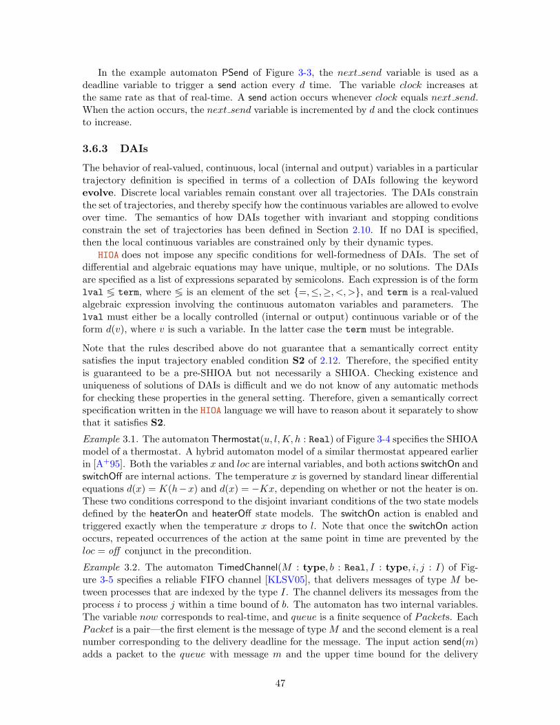
In the example automaton PSend of Figure 3-3, the next send variable is used as adeadline variable to trigger a send action every d time. The variable clock increases atthe same rate as that of real-time. A send action occurs whenever clock equals next send.When the action occurs, the next send variable is incremented by d and the clock continuesto increase.
3.6.3 DAIs
The behavior of real-valued, continuous, local (internal and output) variables in a particulartrajectory definition is specified in terms of a collection of DAIs following the keywordevolve. Discrete local variables remain constant over all trajectories. The DAIs constrainthe set of trajectories, and thereby specify how the continuous variables are allowed to evolveover time. The semantics of how DAIs together with invariant and stopping conditionsconstrain the set of trajectories has been defined in Section 2.10. If no DAI is specified,then the local continuous variables are constrained only by their dynamic types.
HIOA does not impose any specific conditions for well-formedness of DAIs. The set ofdifferential and algebraic equations may have unique, multiple, or no solutions. The DAIsare specified as a list of expressions separated by semicolons. Each expression is of the formlval ≶ term, where ≶ is an element of the set =,≤,≥, <,>, and term is a real-valuedalgebraic expression involving the continuous automaton variables and parameters. Thelval must either be a locally controlled (internal or output) continuous variable or of theform d(v), where v is such a variable. In the latter case the term must be integrable.
Note that the rules described above do not guarantee that a semantically correct entitysatisfies the input trajectory enabled condition S2 of 2.12. Therefore, the specified entityis guaranteed to be a pre-SHIOA but not necessarily a SHIOA. Checking existence anduniqueness of solutions of DAIs is difficult and we do not know of any automatic methodsfor checking these properties in the general setting. Therefore, given a semantically correctspecification written in the HIOA language we will have to reason about it separately to showthat it satisfies S2.
Example 3.1. The automaton Thermostat(u, l,K, h : Real) of Figure 3-4 specifies the SHIOAmodel of a thermostat. A hybrid automaton model of a similar thermostat appeared earlierin [A+95]. Both the variables x and loc are internal variables, and both actions switchOn andswitchOff are internal actions. The temperature x is governed by standard linear differentialequations d(x) = K(h−x) and d(x) = −Kx, depending on whether or not the heater is on.These two conditions correspond to the disjoint invariant conditions of the two state modelsdefined by the heaterOn and heaterOff state models. The switchOn action is enabled andtriggered exactly when the temperature x drops to l. Note that once the switchOn actionoccurs, repeated occurrences of the action at the same point in time are prevented by theloc = off conjunct in the precondition.
Example 3.2. The automaton TimedChannel(M : type, b : Real, I : type, i, j : I) of Fig-ure 3-5 specifies a reliable FIFO channel [KLSV05], that delivers messages of type M be-tween processes that are indexed by the type I. The channel delivers its messages from theprocess i to process j within a time bound of b. The automaton has two internal variables.The variable now corresponds to real-time, and queue is a finite sequence of Packets. EachPacket is a pair—the first element is the message of type M and the second element is a realnumber corresponding to the delivery deadline for the message. The input action send(m)adds a packet to the queue with message m and the upper time bound for the delivery
47

1 automaton Thermostat(u, l,K, h : Real) where u > ltype Status enumeration [on, off ]
3 signatureinternal switchOn; switchOff
5
variables7 internal x : Real := u; loc : Status := on;
9 transitionsinternal switchOn
11 pre x = l ∧ loc = off ;eff loc := on;
13
internal switchOff15 pre x = u ∧ loc = on;
eff loc := off ;
18trajectoriestrajdef heaterOn
20invariant x ≤ u ∧ loc = on;stop when x = u;
22evolve d(x) = K × (h− x);
24trajdef heaterOffinvariant x ≥ l ∧ loc = off ;
26stop when x = l;evolve d(x) = −Kx;
Figure 3-4: Thermostat.
of the message. The output action receive(m) can occur whenever there is a packet withmessage m at the head of the queue and it must occur before now exceeds the deadline forthe message.
1 vocabulary Packet(T :type)types
3 Packet = Tuple [message : T ,deadline : AugmentedReal]
5 end
7 automaton TimedChannel(M :type, b : RealI :type, i, j : I) where b ≥ 0
9 imports Packet(M)signature
11 input send(m : M, const i, j)output receive(m : M, const i, j)
13
variables15 internal queue : Seq[Packet] := ;
16now : Real := 0
18transitionsinput send(m, i, j)
20eff queue := queue ` [m,now + b];
22output receive(m, i, j)pre head(queue).message = m;
24eff queue := tail(queue);
26trajectoriestrajdef timePassage
28stop when head(queue).deadline = nowevolve d(now) = 1;
Figure 3-5: Time-bounded channel.
Example 3.3. The automaton ClockSync(u, ρ : Real, I : type, i : I) of Figure 3-6 specifiesprocesses participating in a distributed clock synchronization algorithm. The physical clock(the variable clock) of each process drifts at a bounded rate of ρ, and the processes com-municate to ensure that their logical clocks (the variable logclock) are close to one anotherand also close to their physical clocks. This example is taken from [KLSV05], where theauthors prove through invariant assertions that the participating processes indeed satisfythe above requirements.
The processes are indexed by elements of type I. The synchronization algorithm isbased on the exchange of physical clock values between different processes in the systemthrough TimedChannels. A process uses its real-valued, discrete variable maxother to keeptrack of the largest physical clock value of other processes in the system. For ClockSync(i),the parameter i of the send action is a constant while the parameter j is a variable. ThusClockSync(i) can send messages to, and receive messages from ClockSync(j), for all j in I,j 6= i. The trajectory specification consists of a single trajectory definition timeElapse. Thisspecifies the evolution of the continuous variable clock using two differential inclusions that
48

bound the drift. The stopping condition ensures that the deadline imposed by nextsend isnot crossed.
1 automaton ClockSync(u, ρ : Real, I :type, i : I)where 0 ≤ ρ ≤ 1 ∧u > 0
3 signatureoutput send(m : Real, const i, j : I) where i 6= j
5 input receive(m : Real, j : I, const i) where i 6= j
7 variablesinternal clock : Real := 0;
9 nextsend : Discrete Real := 0;maxother : Discrete Real := 0;
11 let logclock = max(maxother, clock);
13transitionsoutput send(m, i, j)
15pre m = clock ∧ clock = nextsend;eff nextsend = nextsend+ u;
17
input receive(m, j, i)19eff maxother = max(maxother,m);
21trajectoriestrajdef timeElapse
23stop when clock = nextsendevolve d(clock) ≤ (1 + ρ);
25d(clock) ≥ (1− ρ);
Figure 3-6: Process participating in a clock synchronization algorithm.
3.7 Operations and Properties
In specifying a complex system with many logical pieces, it is convenient to model eachpiece as a separate SHIOA. Then the whole system is specified as a composition of thecomponent SHIOAs. In section 2.4.4 we defined the composition operation for SHIOAs.Here we describe the the HIOA language constructs for specifying compositions and forasserting properties of automata.
3.7.1 Composition
A composed automaton is specified by the automaton name followed by the keyword com-ponents and a semicolon-separated list of component names and automaton types. Forexample, using the TimedChannel and ClockSync automata from the previous section wecan define the composed automaton:
automaton Sync(u, ρ, b : Real, I :type)componentsP [i : I] : ClockSync(u, ρ, I, i);C[i, j : I] : TimedChannel(b, I, i, j) where i 6= j
The keyword components introduces a list of named components: one ClockSync(u, ρ, I, i)automaton, P [i], for each i of type I, and one TimedChannel(b, I, i, j) automaton C[i, j], foreach i, j of type I, such that i 6= j. If the input action of one component has the same nameas the output action of another component, then they are identified and the compositionhas the resulting output action. Likewise, the names of input and output variables areidentified and the composed automaton has the corresponding output variables.
A parameterized automaton specification defines a set of automata rather than a singleautomaton. The composition operation can be used to instantiate a particular automaton.For example, the Sync automaton above defines a set of composed automata for differentparameter types I. We can fix the type parameter to a particular index set a, b, c, d asfollows:
vocabulary types abcd = Enumeration [a, b, c, d] endautomaton Sync4(u, ρ, b : Real)
components theOnly : Sync(u, ρ, b, abcd)
49
3.7.2 Property Assertions
Along with specifications, properties of automata can also be asserted in HIOA. Such asser-tions must appear after the automaton specification. An invariant property of an automatonis stated by the keywords invariant of, followed by the name of the automaton and a pred-icate on the variables of the automaton.
invariant of Sync : ∀ i, j : I, |P [i].logclock − P [j].logclock| ≤ u+ b× (1 + ρ)
A simulation relation is a relation over the states of a pair of HIOAs and it provides a soundway of proving implementation relations (defined in Section 2.2.2). We shall encounterdifferent kinds of simulation relations and study their properties in Chapters 4 and 5. Fornow, we note that simulation relations can also be specified in the HIOA language usingthe simulation from keywords. We conclude the presentation of the HIOA language withanother example which uses many of its features.
Example 3.4. This failure detector example is taken from [KLSV05]; mechanized proofsof correctness appeared in [ALL+06]. The automaton Spec(d) of Figure 3-7 abstractlyspecifies the timing related requirements of a simple failure detector. It specifies that atimeout occurs within d time of a fail. Furthermore, a timeout occurs only if it is precededby a fail. Specifically, the value of failed is initially f alse. Thus, the value of the clockvariable increases indefinitely at the same rate as that of real-time. The fail action canoccur at any point in time. When it does occur, the variable failed is set to true and thedeadline variable last timeout is set to clock + d. This enables the timeout action. Thetrajectory definition failed becomes active and the clock continues to increase at the samerate, but now it can increase only to the point where it equals last timeout. When theclock reaches this value the timeout action must occur. This action sets suspected to true,which in turn once again enables time to elapse indefinitely.
automaton Spec(d : Real) where d > 0signature
input failoutput timeout
variablesinternal last timeout : AugmentedReal := ∞,clock : Real := 0;suspected : Bool := f alse;failed : Bool := f alse;
transitionsinput fail
eff if ¬failedthen last timeout := clock + d;failed := true; fi
output timeoutpre failed ∧¬suspected;eff suspected := true;last timeout := ∞;
trajectoriestrajdef normal
invariant ¬failed ∨ (failed ∧ suspected)evolve d(clock) = 1;
trajdef failedinvariant failed ∧¬suspectedstop when clock = lasttimeoutevolve d(clock) = 1;
Figure 3-7: Failure detector specification.
The automata in Figure 3-8 implement a failure detector using the TimedChannel ofFigure 3-5. PeriodicSend(M,u1) sends a message once every u1 time units, until a fail actionoccurs. This periodic timing is maintained by the next send deadline variable. Notice howthe AugmentedReal type of this variable becomes useful when the fail action occurs.
The messages from PeriodicSend(M,u1) are transmitted over a channel that connectsthis process with the Detector process and delivers every sent message within b time units.In the composite specification Timeout of Figure 3-9, a single TimedChannel is instantiated
50

with the index set 1, 2. The Detector(u2) automaton receives messages from the channel.If it does not receive anything over an u2 time-interval, then it performs a timeout anddeclares PeriodicSend to be suspected to have failed. The next recv variable is used topostpone and then if necessary trigger, the timeout action.
automaton PeriodicSend(M : type, u1 : Real)where u1 ≥ 0
signatureoutput send(m : M)input fail
variablesinternal next send : AugmentedReal := 0;failed : Bool := f alse;clock : Real := 0;
transitionsoutput send(m, 1, 2)
pre clock = next send ∧¬failed;eff next send := clock + u1;
input faileff if ¬failed thenfailed := true; next send := ∞; fi
trajectoriestrajdef normal
stop when clock ≥ next sendevolve d(clock) = 1
automaton Detector(M : type, u2 : Real)where u2 > 0
signatureinput receive(m : M, 1, 2)output timedout
variablesinternal next recv : AugmentedReal := u2;suspected : Bool := f alse;clock : Real := 0
transitionsinput receive(m, 1, 2)
eff next recv := clock + u2
output timedoutpre ¬suspected ∧ clock = next recveff suspected := true;next recv := ∞
trajectoriestrajdef normal
stop when 6= suspected ∧ clock ≥ next recvevolve d(clock) = 1
Figure 3-8: Periodic sender and simple failure detector.
Figure 3-9 also presents two key invariants and a partial statement of the simulationrelation from Timeout to Spec, which are used for proving that Timeout implements Spec.In Chapter 6 we show how HIOA specifications can be translated to the language of the
automaton Timeout(M : type, u1, u2, b : Real) where u1 ≥ 0 ∧u2 ≥ 0 ∧ b ≥ 0 ∧u2 ≥ (u1 + b)components
Sender:PeriodicSend(M,u1);Detector:Detector(M,u2);Channel:TimedChannel(M, b, 1, 2, 1, 2);
invariant of Timeout: ¬Detector.suspected⇒ Detector.next recv ≤ Detector.clock + u2invariant of Timeout: Detector.suspected⇒ Sender.failed. . .forward simulation from Timeout(u1, u2, b) to Spec(d):
(Timeout. Sender.failed = Spec.failed ∧Timeout.Detector.suspected = Spec.suspected ∧. . .)
end
Figure 3-9: Composed automaton and property assertions.
PVS Theorem prover [ORR+96] and how invariant properties and simulation relations canbe proved partially automatically using specially designed proof strategies.
51

3.8 Summary
We described the HIOA language for specifying a general class hybrid systems modeled asSHIOAs. In Section 7.7 a slightly extended version of HIOA is described which allows speci-fication of probabilistic transitions. In addition to all examples in this thesis HIOA has beenused to specify mobile robot coordination algorithms [LMN], cardiac cell models [GMY+07],an air-traffic control system [UL07], and several real-time distributed algorithms [FDGL07].
52
Chapter 4
Verifying Safety Properties
In this chapter we present techniques for verifying safety properties of SHIOAs. A safetyproperty S is a predicate on state variables and an SHIOA A is said to be safe with respectto S, if ReachA ⊆ S, that is, if S is an invariant for A. In other words, A is unsafe ifthere are executions of A that reach some “bad state” in Sc. We present an overview ofexisting work in automatic invariance verification in Section 4.1. In Sections 4.2 and 4.3,we present our deductive approach for verifying invariance and implementation relations.Sections 4.4 and 4.4.2 are dedicated to a case study—a supervisory controller for a helicoptertestbed—which illustrates modeling and safety verification in the SHIOA framework.
4.1 An Overview
Definition 4.1. Let A be a pre-SHIOA with set of internal variables X and set of statesQ ⊆ val(X), and let I be a predicate on X. The set of states satisfying I is also denotedby I. The predicate I is said to be an invariant of A if ReachA ⊆ I.
An SHIOA A is safe with respect to a particular safety property I, if I is an invariantfor A. Given A and a predicate I on X, how do we verify that I is an invariant of A? If theset of reachable states of A, ReachA, is computable then we could check if ReachA ⊆ I. Ithas been known since [HKPV95] that computing ReachA, is decidable only if A belongs to afairly restricted class, such as the class of rectangular, initialized SHIOAs. Other decidableclasses of hybrid automata with linear, polynomial, and exponential state models have beenidentified (see, reachability related papers in [TG02, MP03, AP04, MT05, HT06]). Thesedecidable classes are generally called order minimal or o-minimal hybrid automata [LPY99].The notion of o-minimality comes from mathematical logic. Informally, A theory of realnumbers is said to be o-minimal if every definable subset of R is a finite union of pointsand intervals. Then, a hybrid system is o-minimal, if its initial states, preconditions, resetmaps, invariant sets, stopping conditions, and DAIs are all definable in the same o-minimaltheory.
Another alternative is to compute an overapproximation of ReachA, say ReachA, andthen check if ReachA ⊆ I. If true then I is verified, otherwise one has to check if the statesin ReachA∩I are really reachable or if they are false-positives generated by the overapprox-imation. In the latter case ReachA is iteratively refined. Algorithms for overapproximatingReachA for general hybrid systems have been developed (see, for example, [BCT02]), butmaking these techniques scale remains a challenge.
53

In practice, therefore, a compromise has to be made between the expressive power of theclass of SHIOA that we use for specifying the system and the degree of automation we canhope to achieve in verifying safety. Compared to above mentioned approaches, we opt fora different trade-off between automation and expressive power. We develop invariant prooftechniques that are not always automatic but are applicable to general SHIOAs. Moreover,because a set pattern of steps are always executed in constructing these invariant proofs,the process can be at least partially automated.
4.2 Proving Invariants
We deduce the desired invariant property I from the specification of A by (a) finding aninductive property I ′ ⊆ I, and (b) checking that the transitions and trajectories of Apreserve I ′. This technique has been applied earlier in the context of HIOA for verifyingsafety of air-traffic control systems [LLL99] and vehicle control systems [Lyn96a, WL96,WLD95]. We adapt these techniques to SHIOA and in Chapter 6 we develop theorem prover-based support for partially automating step (b). In order to prove invariant properties, weintroduce another class of properties of A.
Definition 4.2. Let A be a pre-SHIOA with set of internal variables X and set of statesQ ⊆ val(X). A predicate I on X is an inductive property of A if any execution that startsfrom a state satisfying I reaches only states that also satisfy I.
An inductive property that is satisfied by all starting states of A is an invariant. Induc-tive properties can be verified by checking that each transition and trajectory of A preservesthe property. The following lemma which is an adaptation of the classical inductive proofschema a la Floyd [Flo67] to the HIOA setting, formalizes this verification task.
Lemma 4.1. Given an HIOA A, the set of states I ⊆ Q is an invariant of A if it satisfies:
1. (Start condition) For any starting state x ∈ Θ, x ∈ I.
2. (Transition condition) For any action a ∈ A, if x a→ x′ and x ∈ I then x′ ∈ I.
3. (Trajectory condition) For any trajectory τ ∈ T , if τ.fstate ∈ I then τ.lstate ∈ I.
Proof. It suffices to show that ReachA ⊆ I. Consider any reachable state x ∈ ReachA. Bythe definition of a reachable state, there exists an execution α of A such that α.lstate = x.We proceed by induction on the length of the execution α. For the base case, α consists ofa single starting state x ∈ Θ and by the start condition, x ∈ I. For the inductive step, weconsider two subcases:
Case 1: α = α′ax where a is an action of A. By the induction hypothesis we know thatα′.lstate ∈ I. Invoking the transition condition, we obtain x ∈ I.
Case 2: α = α′τ where τ is a trajectory of A and τ.lstate = x. By the induction hypothe-sis, α′.lstate ∈ I and invoking the trajectory condition we deduce that τ.lstate = x ∈I.
54

This technique has been applied to verify safety properties of several hybrid systems(see, for example, [LLL99, LL96, WL96, DL97, WLD95, Lyn96a], and [HL94]). A similarlemma exists for verifying invariant properties of pre-SHIOAs. In practice, the state modelstructure of SHIOAs is useful for verifying the trajectory condition through case analysisof the state models.
Lemma 4.2. Given a pre-SHIOA A, the set of states I ⊆ Q is an invariant of A if itsatisfies:
1. (Start condition) For any starting state x ∈ Θ, x ∈ I.
2. (Transition condition) For any action a ∈ A, if x a→ x′ and x ∈ I then x′ ∈ I.
3. (Trajectory condition) For any state model S ∈ S , any trajectory τ ∈ trajs(S), ifτ.fstate ∈ I then τ.lstate ∈ I.
Proof. It suffices to show that ReachA ⊆ I. For any state x ∈ ReachA there exists anexecution α of A such that α.lstate = x. The proof is by induction on the length of theexecution α. For the base case, α is consisting of a single starting state x ∈ Θ and by thestart condition, x ∈ I. For the inductive step, we consider two subcases:
Case 1: α = α′ax where a is an action of A. By the induction hypothesis we know thatα′.lstate ∈ I. Invoking the transition condition we obtain x ∈ I.
Case 2: α = α′τ where τ is a trajectory of A and τ.lstate = x. By the induction hy-pothesis, α′.lstate ∈ I. Since τ is a trajectory of A, it follows that there exists astate model S such that τ ∈ trajs(S). Invoking the trajectory condition we get thatτ.lstate = x ∈ I.
Often, it is convenient to prove invariants for SHIOAs which are components of a larger,composed system. The following result ensures that any invariant for a component SHIOAcarries over to the composed system.
Lemma 4.3. Suppose A1 and A2 are compatible pre-SHIOAs. If I is an invariant forpre-SHIOA A1 then I ×Q2 is an invariant for A1||A2.
Proof. First we show that ReachA1||A2d X1 ⊆ ReachA1 . Fix a state x ∈ ReachA1||A2
d X1.We know that there exists a closed execution α of A1||A2 such that α.lstate = x. FromLemma 2.2, α d (A1, V1) is an execution ofA1. Further, α.lstate d X1 = (α d (A1, V1)).lstatewhich is a reachable state of A1. Thus, ReachA1||A2
d X1 ⊆ ReachA1 . Since I is an invariantfor A1, ReachA1 ⊆ I and therefore, ReachA1||A2
d X1 ⊆ I. As I is independent of thevariables of A2, it follows that ReachA1||A2
⊆ I ×Q2. That is, I ×Q2 is an invariant of thecomposed automaton A1||A2.
4.3 Proving Implementation Relations
Many different kinds of implementation or abstraction relations and their correspondingproof methods have been developed for timed [AD94] and hybrid automata [KLSV05,TK02, TPL02]. For restricted classes hybrid systems, such as o-minimal hybrid automata,
55

automatic techniques exist for proving implementation relations, particularly bisimulationrelations. As in the case of invariant verification, our approach here is to develop prooftechniques that are applicable to the general class of SHIOAs.
Implementation relations (see Definition 2.13) are proved by demonstrating the existenceof a simulation relation between the concerned pair of automata. The following definitionof forward simulation relation and the corresponding soundness theorem were presentedin [LSV03], in the context of HIOAs. Since implementation of pre-SHIOAs is defined interms of the implementation of the corresponding pre-HIOAs, the soundness result extendsto the case of pre-SHIOAs in a straightforward manner.
Definition 4.3. Consider comparable pre-SHIOAs A and B. A simulation relation fromA to B is a relation R ⊆ QA ×QB satisfying the following conditions, for all states x andy of A and B, respectively:
1. (Start condition) If x ∈ ΘA then there exists a state y ∈ ΘB such that x R y.
2. (Transition condition) If x R y and α is an execution fragment of A consisting ofone single action surrounded by two point trajectories and α.fstate = x, then Bhas a closed execution fragment β with β.fstate = y, trace(β) = trace(α), andα.lstate R β.lstate.
3. (Trajectory condition) If x R y and α is an execution fragment of A with consistingof a single closed trajectory and α.fstate = x, then B has a closed execution fragmentβ with β.fstate = y, trace(β) = trace(α), and α.lstate R β.lstate.
Theorem 4.4. Let A and B be comparable pre-SHIOAs and let R be a simulation relationfrom A to B. Then A ≤ B.
4.4 Case Study: Safety Verification of Helicopter Testbed
In this section and the next, we present the safety verification of a supervisory controllerfor a helicopter testbed using the techniques presented in Section 4.2. First, we present theHIOA specification of the components of the system and the safety property of interest. Thisexample showcases several features of the HIOA language. Then, in Section 4.4.2, we presentthe safety verification of the system. Verification involves proving a sequence of intermediateinvariants and lemmas. Almost all the intermediate invariants are proved using Lemma 4.2;the remaining are deduced using other, already proved, invariants and the lemmas thatassert timing related behavior of the SHIOAs. Invariant properties of the whole system arederived from those of the components of the system by applying Lemma 4.3. The proofsusing Lemma 4.2 illustrate how stylized hand-proofs of invariant properties are constructedby systematic analysis of SHIOA specifications—a first step toward automation in deductiveverification. In chapter 6 we will discuss how stylized proofs of this kind can be constructedpartially automated using mechanical theorem provers.
This case study appeared earlier in [MWLF03]. The helicopter testbed manufactured byQuanser [Qua] (see Figure 4.4) is driven by two rotors mounted at the two ends of its frame.The frame is suspended from an instrumented joint which in turn is mounted at the end ofa long arm. The arm is gimbaled on another instrumented joint and is free to pitch andyaw, giving the helicopter three degrees of freedom. The rotor inputs are either controlledby the user with a joystick, or through software controllers. A complete dynamical model
56

frame
rotor
long arm
instrumented joint #2
instrumented joint #1
qpitch angle
counterweight
Figure 4-1: Helicopter testbed manufactured by Quanser Inc.
of the helicopter with three degrees of rotational freedom appears in [WIM+02]. Here weconsider the pitch dynamics of the helicopter, which are critical for safety. In practice, theroll and yaw effects are eliminated by making the initial conditions along these axes to bezero and giving identical input to the two rotors. The magnitude of the total input to thepitch axis is always restricted to be within [umin, umax] units. If the pitch angle θ is toolarge the arm stresses the instrumented joint, and if it is too small then the frame hits theground causing physical damage. The system is safe if the pitch angle remains within arange [θmin, θmax] that avoids these extremes.
A supervisory controller is designed to prevent the helicopter from reaching unsafe states.It periodically observes the pitch angle and the pitch velocity of the helicopter, conserva-tively estimates the worst that may happen if the user is allowed to remain in control,and when necessary for ensuring safety, overrides the user’s output with a suitable alter-native output. The design of the supervisor is constrained by the actuator bandwidth, thesampling rate, and the sensor inaccuracies. In section 4.4.1, we present the SHIOA specifi-cations of the components that make up the helicopter testbed and state basic properties ofthese components. In section 4.4.2, we present the verification of the safety of the completesystem through a sequence of invariant assertions.
4.4.1 System Specification
Figure 4-2 shows the component SHIOAs of the helicopter testbed, their key state variables,and their interactions through input/output variables and actions. The formal parametersof the actions are not shown in this figure. The helicopter system is the composition ofHelicopter, Sensor, UsrCtrl, Actuator, and Supervisor. The resulting composed automaton Ais also a SHIOA. Some of these component automata have state variables with the samename (for example, θ0 and θ1). As the set of local variables are required to be disjoint forthe automata to be compatible, we rename the overlapping variable names by adding thefirst letter of the component automaton as a suffix. For the Supervisor automaton we usethe suffix c, instead of s.
57

Helicopter
θ0h, θ1h
Sensor
θ0s , θ1s ,
next sample
Actuator
buffer , ua
UsrCtrl
uu
Supervisor
mode, θ0c , θ1c , uc
θ0, θ1
sampleusrOutput
sample
supOutput
u
dequeue
Figure 4-2: Interconnection of SHIOA components in Quanser helicopter system.
Helicopter
The Helicopter SHIOA (Figure 4-3) specifies pitch dynamics of the helicopter with respect tothe rotor input voltage u. This automaton does not contain actions or discrete transitions.Its state evolves according to the differential equation: d(θ1
h) + Ω2 cos θ0h = u, which relates
the pitch angle θ0h, the pitch velocity θ1
h, the characteristic frequency of the system Ω, andthe net rotor input u for the pitch axis. The output variables θ0 and θ1, which are simplycopies of θ0
h and θ1h, are used for communicating the state of the helicopter to a sensor. The
Helicopter is safe if the pitch angle θ0h is within θmin and θmax. The set of safe states S for
the composed SHIOA A, is defined as:
S∆= x ∈ QA | θmin ≤ x d θ0
h ≤ θmax. (4.1)
automaton Helicopter(Ω : Real) where Ω > 0variables
input u : Real;output θ0 : Real; θ1 : Real;
internal θ0h : Real := 0; θ1h : Real := 0;
trajectoriestrajdef pitchDynamics
evolve d(θ0h) = θ1h; d(θ1h) = −Ω2 cos(θ0h) + u;
θ0 = θ0h; θ1 = θ1h;
Figure 4-3: Quanser helicopter pitch dynamics.
Sensor
The Sensor automaton (Figure 4-4) models a sensor that reads the pitch angle θ0 andthe pitch velocity θ1 and produces noisy estimates of these quantities, once every ds > 0time units. Although the estimates are inaccurate, they are guaranteed to be within ±e0and ±e1 units of the actual values of θ0 and θ1, respectively. The estimates for θ0, θ1are encapsulated as the parameters x0, x1 of the sample action. The clock variable nowsand the deadline variable next sample are used to periodically trigger the sample action
58

automaton Sensor(e0, e1, ds : Real)where e0, e1, ds > 0
signatureoutput sample(x0, x1 : Real)
variablesinput θ0 : Real; θ1 : Real;
internal θ0s : Real; θ1s : Real;nows : Real := 0;next sample : AugmentedReal := ds;let time left := next sample− nows
transitionsoutput sample(x0, x1)
pre nows = next sample
∧x0 ∈ [θ0s − e0, θ0s + e0]
∧x1 ∈ [θ1s − e1, θ1s + e1];eff next sample := next sample+ ds;
trajectoriestrajdef periodicSample
stop when nows = next sample
evolve d(nows) = 1; θ0s = θ0; θ1s = θ1;
Figure 4-4: Periodic noisy sensor.
in a manner that is similar to the PSend automaton of Figure 3-3. When next sampleequals nows a set of sample(x0, x1) actions are enabled—one for each x0 ∈ [θ0
s − e0, θ0s + e0]
and x1 ∈ [θ1s − e1, θ
1s + e1]. Out of all these enabled actions, one particular is chosen
nondeterministically. This choice captures the uncertainty in the sensor readings.Invariant 4.5 captures a key property of Sensor, namely, that the value of the time left
variable (measuring time left to the next sample action) is bounded within 0 and ds.
Invariant 4.5. In every reachable state of Sensor, 0 ≤ time left ≤ ds.
Proof. By a straightforward application of Lemma 4.2 it follows that 0 ≤ next sample −nows ≤ ds is an invariant. This suffices because the derived variable time left is defined tobe equal to next sample− nows.
User-defined Controller
The UsrCtrl automaton (Figure 4-5) models an arbitrary user controller. UsrCtrl receives pe-riodic estimates of the helicopter’s state from Sensor through the sample action and respondsimmediately with a usrOutput(u′) action. The parameter u′ of the action corresponds touser’s choice of input to the helicopter. This choice is modeled by the nondeterministicassignment to the variable uu over the range [umin, umax] in the effect of Sample. The flagvariable readyu indicates that the sample action has occurred. Similar flags are used insome of the subsequent specifications as well; these variables do not influence the behav-ior of automata, however by augmenting information content of state, they aid inductiveinvariant proofs (see, for example, the proof of 4.8).
It is worth remarking that UsrCtrl is a rather abstractly specified user controller which iscapable of issuing arbitrarily inputs to the helicopter. A supervisor that ensures safety of thehelicopter system with UsrCtrl guarantees safety with respect to any other user controller,because every possible controller implements UsrCtrl. Given a concrete user controller, aformal proof of such a statement can be constructed by applying Theorem 4.4.
Supervisor
The Supervisor automaton (Figure 4-7) models the switched supervisory controller thatwe have developed for ensuring safety of the helicopter. A second requirement for theSupervisor is to interfere as little as possible with the user controller. There are well knownalgorithms [FK98, ABD+00, LTS99] for synthesizing controllers for linear hybrid systems.
59
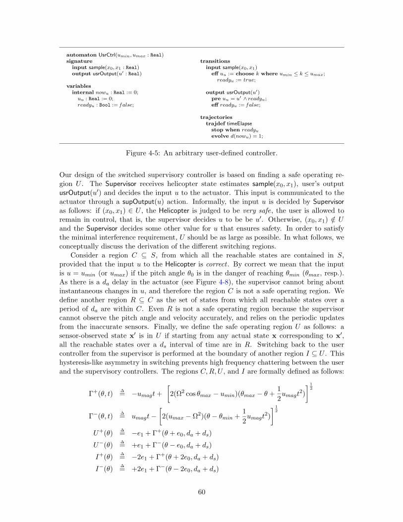
automaton UsrCtrl(umin, umax : Real)signature
input sample(x0, x1 : Real)output usrOutput(u′ : Real)
variablesinternal nowu : Real := 0;uu : Real := 0;readyu : Bool := f alse;
transitionsinput sample(x0, x1)
eff uu := choose k where umin ≤ k ≤ umax;readyu := true;
output usrOutput(u′)pre uu = u′ ∧ readyu;eff readyu := f alse;
trajectoriestrajdef timeElapse
stop when readyu
evolve d(nowu) = 1;
Figure 4-5: An arbitrary user-defined controller.
Our design of the switched supervisory controller is based on finding a safe operating re-gion U . The Supervisor receives helicopter state estimates sample(x0, x1), user’s outputusrOutput(u′) and decides the input u to the actuator. This input is communicated to theactuator through a supOutput(u) action. Informally, the input u is decided by Supervisoras follows: if (x0, x1) ∈ U , the Helicopter is judged to be very safe, the user is allowed toremain in control, that is, the supervisor decides u to be be u′. Otherwise, (x0, x1) /∈ Uand the Supervisor decides some other value for u that ensures safety. In order to satisfythe minimal interference requirement, U should be as large as possible. In what follows, weconceptually discuss the derivation of the different switching regions.
Consider a region C ⊆ S, from which all the reachable states are contained in S,provided that the input u to the Helicopter is correct . By correct we mean that the inputis u = umin (or umax) if the pitch angle θ0 is in the danger of reaching θmin (θmax, resp.).As there is a da delay in the actuator (see Figure 4-8), the supervisor cannot bring aboutinstantaneous changes in u, and therefore the region C is not a safe operating region. Wedefine another region R ⊆ C as the set of states from which all reachable states over aperiod of da are within C. Even R is not a safe operating region because the supervisorcannot observe the pitch angle and velocity accurately, and relies on the periodic updatesfrom the inaccurate sensors. Finally, we define the safe operating region U as follows: asensor-observed state x′ is in U if starting from any actual state x corresponding to x′,all the reachable states over a ds interval of time are in R. Switching back to the usercontroller from the supervisor is performed at the boundary of another region I ⊆ U . Thishysteresis-like asymmetry in switching prevents high frequency chattering between the userand the supervisory controllers. The regions C,R,U , and I are formally defined as follows:
Γ+(θ, t) ∆= −umagt+[2(Ω2 cos θmax − umin)(θmax − θ +
12umagt
2)] 1
2
Γ−(θ, t) ∆= umagt−[2(umax − Ω2)(θ − θmin +
12umagt
2)] 1
2
U+(θ) ∆= −e1 + Γ+(θ + e0, da + ds)
U−(θ) ∆= +e1 + Γ−(θ − e0, da + ds)
I+(θ) ∆= −2e1 + Γ+(θ + 2e0, da + ds)
I−(θ) ∆= +2e1 + Γ−(θ − 2e0, da + ds)
60

θ0
θ1
C+
R+
U+
I+
C−
R−U−I−
S
C
RU
I
Figure 4-6: Switching regions of supervisory controller.
C∆= x ∈ QA | x d θ0
h ∈ [θmin, θmax],x d θ1h ∈ [Γ−(x d θ0
h, 0),Γ+(x d θ0h, 0)] (4.2)
R∆= x ∈ QA | x d θ0
h ∈ [θmin, θmax],x d θ1h ∈ [Γ−(x d θ0
h, da),Γ+(x d θ0
h, da)] (4.3)
U∆= x ∈ QA | x d θ0
c ∈ [θmin + e0, θmax − e0],x d θ1c ∈ [U−(x d θ0
c ), U+(x d θ0
c )] (4.4)
I∆= x ∈ QA | x d θ0
c ∈ [θmin + e0, θmax − e0],x d θ1c ∈ [I−(x d θ0
c ), I+(x d θ0
c )] (4.5)
Here umag = umax−umin. The shapes of these regions are as shown in Figure 4-6 for typicalvalues of the parameters umag, da, ds, e0, and e1. The Supervisor reads the sensor-estimatedhelicopter state through sample(x0, x1) and copies x0, x1 into internal variables θ0
c and θ1c .
Based on this state information, the value of the tentative output usup is decided. If thepitch velocity θ1
c is greater than or equal to I+(θ0c ), then usup is set to be umax and if θ0
c isless than I−(θ0
c ) then usup is set to be umin. Otherwise, the value of usup is left unchanged.When usrOutput(u′) occurs, u′ is copied into uusr. This action also sets the values of thevariables uc and mode based on the current values of θ0
c , θ1c , and mode. If mode = usr and
the observed state is in U then mode remains unchanged and us = uusr. If mode = usr butthe observed state is not in U then mode is changed to sup and us = usup. If mode = supthen us is copied from usup and mode is set to usr only if (θ0
c , θ1c ) is in I. The following
lemma states the containment relationships among the different switching regions definedby Equations (4.1)-(4.5).
Lemma 4.6. I ⊆ U ⊆ R ⊆ C ⊆ S.
Proof. Follows from the definitions of C,R,U and I.
61
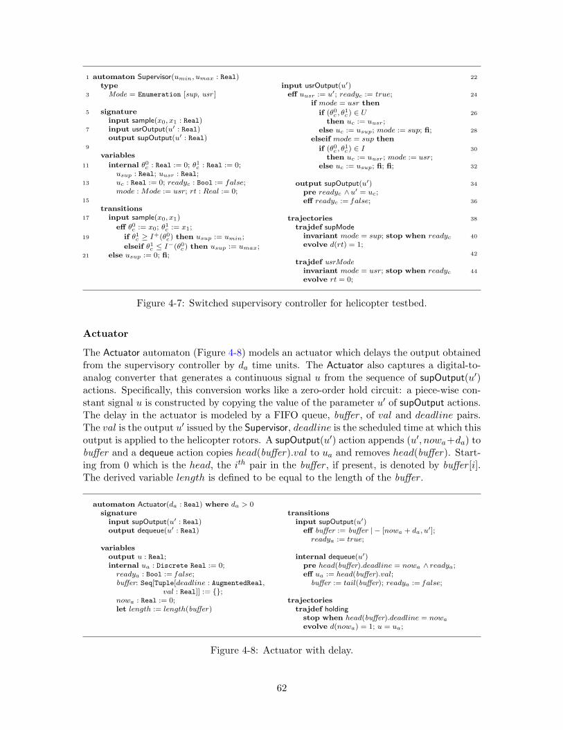
1 automaton Supervisor(umin, umax : Real)type
3 Mode = Enumeration [sup, usr ]
5 signatureinput sample(x0, x1 : Real)
7 input usrOutput(u′ : Real)output supOutput(u′ : Real)
9
variables
11 internal θ0c : Real := 0; θ1c : Real := 0;usup : Real; uusr : Real;
13 uc : Real := 0; readyc : Bool := false;mode : Mode := usr; rt : Real := 0;
15
transitions17 input sample(x0, x1)
eff θ0c := x0; θ1c := x1;
19 if θ1c ≥ I+(θ0c ) then usup := umin;
elseif θ1c ≤ I−(θ0c ) then usup := umax;21 else usup := 0; fi;
22
input usrOutput(u′)24eff uusr := u′; readyc := true;
if mode = usr then
26if (θ0c , θ1c ) ∈ U
then uc := uusr;28else uc := usup; mode := sup; fi;
elseif mode = sup then
30if (θ0c , θ1c ) ∈ I
then uc := uusr; mode := usr;32else uc := usup; fi; fi;
34output supOutput(u′)pre readyc ∧u′ = uc;
36eff readyc := f alse;
38trajectoriestrajdef supMode
40invariant mode = sup; stop when readyc
evolve d(rt) = 1;42
trajdef usrMode44invariant mode = usr; stop when readyc
evolve rt = 0;
Figure 4-7: Switched supervisory controller for helicopter testbed.
Actuator
The Actuator automaton (Figure 4-8) models an actuator which delays the output obtainedfrom the supervisory controller by da time units. The Actuator also captures a digital-to-analog converter that generates a continuous signal u from the sequence of supOutput(u′)actions. Specifically, this conversion works like a zero-order hold circuit: a piece-wise con-stant signal u is constructed by copying the value of the parameter u′ of supOutput actions.The delay in the actuator is modeled by a FIFO queue, buffer , of val and deadline pairs.The val is the output u′ issued by the Supervisor, deadline is the scheduled time at which thisoutput is applied to the helicopter rotors. A supOutput(u′) action appends (u′, nowa+da) tobuffer and a dequeue action copies head(buffer).val to ua and removes head(buffer). Start-ing from 0 which is the head, the ith pair in the buffer , if present, is denoted by buffer [i].The derived variable length is defined to be equal to the length of the buffer .
automaton Actuator(da : Real) where da > 0signature
input supOutput(u′ : Real)output dequeue(u′ : Real)
variablesoutput u : Real;internal ua : Discrete Real := 0;readya : Bool := f alse;buffer: Seq[Tuple[deadline : AugmentedReal,
val : Real]] := ;nowa : Real := 0;let length := length(buffer)
transitionsinput supOutput(u′)
eff buffer := buffer | − [nowa + da, u′];readya := true;
internal dequeue(u′)pre head(buffer).deadline = nowa ∧ readya;eff ua := head(buffer).val;
buffer := tail(buffer); readya := f alse;
trajectoriestrajdef holding
stop when head(buffer).deadline = nowa
evolve d(nowa) = 1; u = ua;
Figure 4-8: Actuator with delay.
62

Invariant 4.7 states that the deadlines corresponding to successive elements in the bufferare non-decreasing, and that all the deadlines are between nowa and nowa + da. This is atypical invariant proof using the induction scheme of Lemma 4.2. Note how the transitionand the trajectory conditions are checked by case analysis of the actions and state modelsof Actuator.
Invariant 4.7. In any reachable state of Actuator, for all 0 ≤ i ≤ length − 1, nowa ≤buffer [i].deadline ≤ buffer [i+ 1].deadline ≤ nowa + da.
Proof. The proof is by an application of Lemma 4.2. The start condition holds vacuouslybecause buffer is empty. For the transition condition, consider a transition x a→ x′ suchthat x d buffer satisfies the above invariant. Consider two subcases:
Case 1: a = dequeue. From the induction hypothesis we know that x d buffer satisfies theinvariant. Since x′ d buffer = tail(x d buffer), it follows that x′ d buffer also satisfiesthe invariant.
Case 2: a = supOutput(u′). From the transition definition, x′ d buffer equals x d bufferwith one additional pair appended to its end. From the induction hypothesis it is clearthat the deadlines for all the elements in buffer , possibly with the exception of thelast one, satisfy the invariant. The deadline for the last element is (x d nowa) + da,which greater than the deadline for the next-to-last element in buffer , and thereforex′ satisfies the invariant.
For the trajectory condition, there is just one case to check because the automaton hasa single state model holding. Consider a closed trajectory τ ∈ trajs(holding), such thatτ.fstate satisfies the invariant. The buffer does not change over the trajectory, τ.fstate dbuffer = τ.lstate d buffer , and nowa increases monotonically at the rate of real-time. Thus,it suffices to check that nowa ≤ head(buffer).deadline at the last state of τ . Supposefor the sake of contradiction τ.lstate d nowa > head(buffer).deadline. Then, there existst ∈ τ.dom, t < τ.ltime, such that (τ ↓ nowa)(t) = head(buffer).deadline. This meansthat τ(t) satisfies the stopping condition for the state model holding and therefore (byDefinition 2.11) t = τ.ltime which contradicts our assumption.
4.4.2 Safety Verification
The composed SHIOA A is safe if the reachable states of A are contained in the safe set S,that is, if S is an invariant property for A. As is often the case, however, invariance of Scannot be directly deduced from the specification of A. For this reason, we find a strongerinvariant property C (defined by Eqution (4.2)).
We verify invariance of C (Theorem 4.22) by proving a sequence of 12 intermediateinvariants and 5 lemmas. We have already seen Invariants 4.7, 4.5, and Lemma 4.6. Lem-mas 4.6, 4.10,and 4.19, and state relationships between various subsets of C that appearin the invariant properties. These relationships are deduced directly by expanding thedefinition of the subsets.
The fourth lemma (Lemma 4.11), characterizes the reachable states over any singletrajectory in the user mode. The proof of this lemma involves integrating the continuousdynamics of the Helicopter with the worst possible user input. The fifth lemma (Lemma 4.8),asserts a property about the time of occurrence of the sample, usrOutput, and the supOutput
63

actions. Such timing properties cannot be formalized as invariants, however, in many in-stances, the design of the system itself suggests a way of proving them. For example, theproof of this Lemma 4.8 is constructed by reasoning about the design of the system, startingfrom key fact that the sample action occurs periodically (Invariant 4.5).
Almost all of the 12 intermediate invariants are proved using the induction scheme ofLemma 4.2; the rest are deduced from other invariants and lemmas. Applying Lemma 4.2involves checking the transition condition and the trajectory condition. Checking the tran-sition conditions involves applying the precondition of the action and the invariant on thepre-state, expanding the definition of the post-state as specified by the HIOA program foreffects, and deducing that the post-state satisfies the invariant. Most often, this followsfrom straightforward simplification of the definition of the invariant, the precondition, andthe post-state. This also suggests that these proof steps can be automated to a fair degreeusing theorem provers (This is the topic of Chapter 6).
In general, checking the trajectory conditions involve solving the DAIs describing thestate models of A. However in our case study, apart from Invariants 4.13, 4.20, and 4.21,the trajectory conditions are verified easily because the variables involved in the invarianteither remain constant over trajectories or they evolve at the constant rate of 1. Theproofs of Invariants 4.13 and 4.20 are based on estimating the largest possible envelope ofreachable states. The trajectory conditions in these proofs are checked by deriving boundson the extreme values of the state variables by integrating the differential equations of theHelicopter pitch dynamics, with worst possible user input. The proof of Invariant 4.21 relieson the fact that the input to the Helicopter is correct (Invariant 4.15). With this extrainformation, the trajectory condition of this invariant is checked by showing that the vectorfield associated with the DAEs of the Helicopter are pointing inwards at the boundary of theinvariant set C. This last technique is based on the subtangential condition for checkinginvariance of continuous time systems as described by Theorem 3.4.11 in [BS67]. Thispresents a systematic way of checking the trajectory condition for hybrid systems withgeneral state models, without requiring the explicit solution of differential equations.
Our verification methodology does not rely on the exact values of the system parametersθmin, θmax, umin, umax, da, and ds, however, these parameters must satisfy the followingrelationships.
θmin < 0 < |θmin| < θmax, umax > Ω2, and umin ≤ 0. (4.6)For any trajectory τ ∈ trajs(A),
τ.fstate d θ1c > I+(τ.fstate d θ0
c ) ⇒ τ.lstate d θ1c ≥ I−(τ.lstate d θ0
c ) (4.7)
τ.fstate d θ1c < I−(τ.fstate d θ0
c ) ⇒ τ.lstate d θ1c ≤ I+(τ.lsate d θ0
c ). (4.8)
Equations (4.6) are consequences of the physical dimensions of the helicopter. Equa-tions (4.7) and (4.8) bound the length of any closed trajectory in terms of the pitch velocityin its first and last states. Indirectly, this bounds the speed of the helicopter with respectto sampling rate (1/ds) of the sensor: the state of the helicopter cannot jump across theregion I in less than ds time. We begin by proving some preliminary properties of A; thenwe proceed to prove safety of A, first in the user mode and finally in the supervisor mode.
64

4.4.3 Preliminary Properties
Automaton A has three state variables called nows, nowa, and nowu, respectively. Each ofthese variables models real-time and their values are always identical. For simplicity, in theremainder of this section we use a single variable called now without any subscript.
The periodic sample action of the Sensor automaton is used to instantly trigger ausrOutput and then a supOutput action. This tight synchronization is formalized by thefollowing lemma.
Lemma 4.8. In any execution of A, sample, usrOutput, and supOutput actions occur whennow = nds, and dequeue actions occur when timer = da + nds for some integer n > 0.
Proof. Initially next sample = ds and every time sample occurs, next sample is incre-mented by ds; next sample always equals nds, where n ∈ N. The predicate now =next sample is the enabling condition for sample and it is also the stopping condition forthe (only) state model periodicSample. Thus, whenever next sample = now = nds, sampleis enabled and since time cannot elapse, sample actually occurs.
As an effect of sample, readyu is set to true. Since readyu is the enabling conditionfor usrOutput and the stopping condition for the state model timeElapse, usrOutput occursimmediately following sample. Similarly, when usrOutput occurs it sets readyc to true andthis forces supOutput to occur immediately.
We have shown that sample, usrOutput, and supOutput always occur in that order, with-out any time delay between them and whenever they occur now = nds. Every supOutputinserts an element in the Actuator buffer , and the deadline associated with the element isnow+da. Thus, for every element in buffer the deadline is of the form nds+da, where n ∈ N.Finally, head(buffer).deadline = now is an enabling condition for dequeue and a stoppingcondition for the state model holding. Therefore dequeue occurs when now = nds + da, forsome n ∈ N.
An element is inserted in the buffer every ds time and it is taken out after da time.Therefore the length of the buffer is bounded. The next invariant uses Lemma 4.8 to limitthe length of the Actuator buffer .
Invariant 4.9. In every reachable state of A, for all 0 ≤ i ≤ length − 2, buffer [i +1].deadline = buffer [i].deadline+ ds, and length ≤ dda
dse.
Proof. From the proof of Lemma 4.8 we know that the deadline for each element in bufferhas value nds + da for some n ∈ N. Furthermore, the difference in the deadlines of twoconsecutive elements is exactly ds. From Invariant 4.7, the difference between the first andthe last deadline is at most da. Therefore, the maximum number of elements in buffer isddadse.
We say that a given state x of A is in the user mode if x d mode = usr and it is inthe supervisor mode if x d mode = sup. In the next section we prove that A is safe in theuser mode, that is, all reachable states that are in the user mode are contained in S. InSection 4.4.5 we shall prove safety in the supervisor mode.
65

4.4.4 User Mode
First, we informally describe the main idea underlying the proof. Consider the followingworst case scenario: a sample action occurs when the Helicopter is at the boundary of U ,say on U+. The supervisor decides to keep mode = usr, and the output from the UsrCtrlcontinues to drive the Helicopter. That is, the output from UsrCtrl enters the Actuatorbuffer , and then the Helicopter after a delay of da time units. This continues for the nextds time units, after which another sample action occurs, and at this point the supervisoronce again gets to decide the mode. Now, what is the worst possible output from UsrCtrlwhich drives the Helicopter for this ds interval ? It is umax. This is because the Helicopteris at U+ at the beginning of the interval, and an input of umax forces the state Helicopterto move most upwards rapidly in the phase-plane. At the next sample point the supervisordetects that the Helicopter is outside U , and starts to feed the appropriate input, namely,umin. But the buffer still contains the umax inputs from UsrCtrl, and it takes some moretime for umin to actually enter. In this time the state goes outside U , but remains (as weshall shortly prove) within a larger safe set R.
In what follows we shall show that the state of the Helicopter remains within R whilethe system is in the user mode. In order to accomplish this through invariant assertions,we define a set of regions At, for each t, 0 ≤ t ≤ ds.
At∆= x | x d θ0
h ∈ [θmin, θmax] ∧ x d θ1h ∈ [Γ−(x d θ0
h, da + t),Γ+(x d θ0h, da + t) (4.9)
The boundaries of the At regions alongside those of R and U are shown in Figure 4-9 (Left).Lemma 4.10 relates the At regions with R and U . Throughout the remainder of this chapter,in all invariant assertions x denotes a reachable state of A.
Lemma 4.10. (i) A0 = R, (ii) U ⊆ Ads, and (iii) for 0 ≤ t ≤ t′ ≤ ds, At′ ⊆ At.
Proof. For part (i), set t = 0 in the definition of At and compare with the definition of R.For part (ii), note that θ0
h ∈ [θ0c − e0, θ
0c + e0] and θ1
h ∈ [θ1c − e1, θ
1c + e1]. Setting t = ds we
have:
Ads = x | x d θ0c ∈ [θmin − ε0, θmax + ε0] ∧ x d θ1c ∈ [Γ−(x d θ0h, da + ds)− ε1,Γ+(x d θ0h, da + ds) + ε1].
Observe that Γ+ and Γ− are monotonically increasing and monotonically decreasing, re-spectively, with respect to θ. Since θ0
h ≥ θ0c − ε0, Γ−(θ0
h, y) ≤ Γ−(θ0c − ε0, y). Similarly,
θ0h ≤ θ0
h + ε0 implies that Γ+(θ0h, y) ≥ Γ+(θ0
c + ε0, y). Therefore,
U = x | x d θ0h ∈ [θmin, θmax] ∧x d θ1h ∈ [Γ−(x d θ0c − ε0, da + ds) + ε1,Γ+(x d θ0c + ε0, da + ds)− ε1] ⊆ Ads .
For part (iii), we observe that in the definition for At, Γ+ and Γ− are monotonically decreas-ing and monotonically increasing, respectively, with respect to t. Therefore if 0 ≤ t ≤ t′ ≤ dsthen At′ ⊆ At.
The proof of safety in the user mode relies on estimating the envelope which containsall states of the Helicopter which can be reached over a ds interval of time, starting fromU , with worst possible user input. The next lemma gives a bound on the reachable statesover a single trajectory in terms of the At sets. This lemma is used to check the trajectorycondition of Invariant 4.12.
66
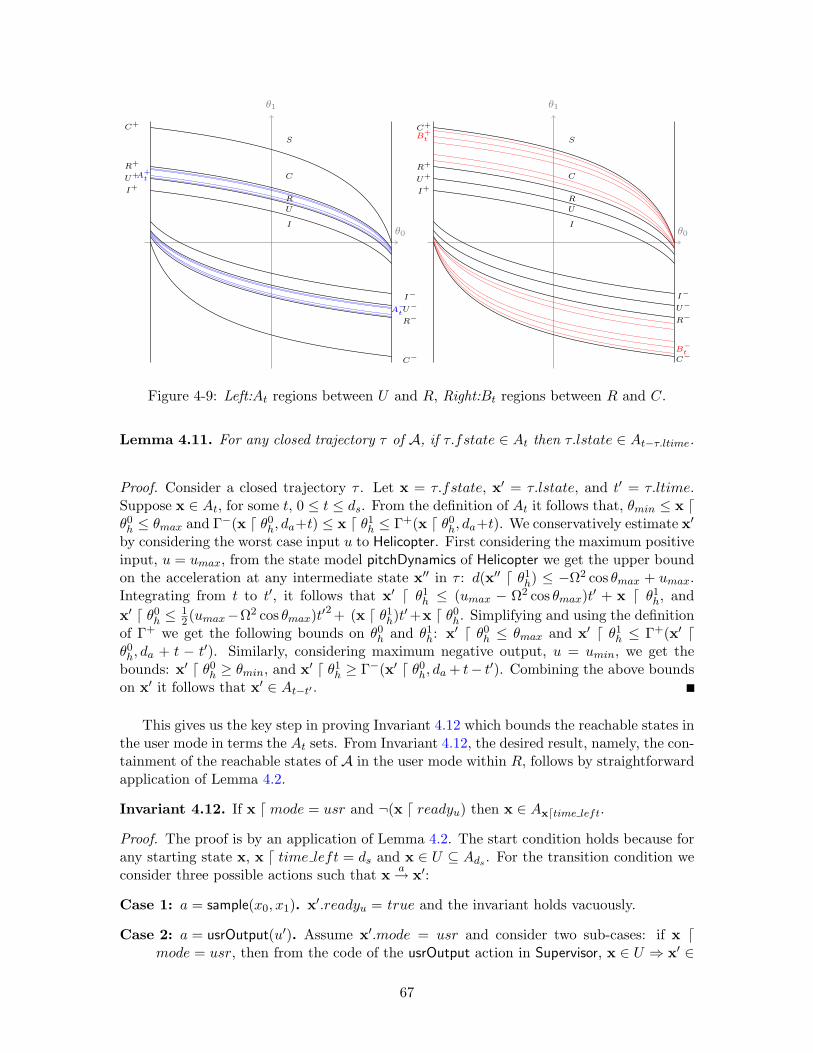
θ0
θ1
C+
R+
A+tU+
I+
C−
R−A−tU−
I−
S
C
R
U
Iθ0
θ1
C+
B+t
R+
U+
I+
C−B−t
R−U−I−
S
C
R
U
I
Figure 4-9: Left:At regions between U and R, Right:Bt regions between R and C.
Lemma 4.11. For any closed trajectory τ of A, if τ.fstate ∈ At then τ.lstate ∈ At−τ.ltime.
Proof. Consider a closed trajectory τ . Let x = τ.fstate, x′ = τ.lstate, and t′ = τ.ltime.Suppose x ∈ At, for some t, 0 ≤ t ≤ ds. From the definition of At it follows that, θmin ≤ x dθ0h ≤ θmax and Γ−(x d θ0
h, da+t) ≤ x d θ1h ≤ Γ+(x d θ0
h, da+t). We conservatively estimate x′
by considering the worst case input u to Helicopter. First considering the maximum positiveinput, u = umax, from the state model pitchDynamics of Helicopter we get the upper boundon the acceleration at any intermediate state x′′ in τ : d(x′′ d θ1
h) ≤ −Ω2 cos θmax + umax.Integrating from t to t′, it follows that x′ d θ1
h ≤ (umax − Ω2 cos θmax)t′ + x d θ1h, and
x′ d θ0h ≤
12(umax−Ω2 cos θmax)t′
2 + (x d θ1h)t
′+x d θ0h. Simplifying and using the definition
of Γ+ we get the following bounds on θ0h and θ1
h: x′ d θ0h ≤ θmax and x′ d θ1
h ≤ Γ+(x′ dθ0h, da + t − t′). Similarly, considering maximum negative output, u = umin, we get the
bounds: x′ d θ0h ≥ θmin, and x′ d θ1
h ≥ Γ−(x′ d θ0h, da + t− t′). Combining the above bounds
on x′ it follows that x′ ∈ At−t′ .
This gives us the key step in proving Invariant 4.12 which bounds the reachable states inthe user mode in terms the At sets. From Invariant 4.12, the desired result, namely, the con-tainment of the reachable states of A in the user mode within R, follows by straightforwardapplication of Lemma 4.2.
Invariant 4.12. If x d mode = usr and ¬(x d readyu) then x ∈ Axdtime left.
Proof. The proof is by an application of Lemma 4.2. The start condition holds because forany starting state x, x d time left = ds and x ∈ U ⊆ Ads . For the transition condition weconsider three possible actions such that x a→ x′:
Case 1: a = sample(x0, x1). x′.readyu = true and the invariant holds vacuously.
Case 2: a = usrOutput(u′). Assume x′.mode = usr and consider two sub-cases: if x dmode = usr, then from the code of the usrOutput action in Supervisor, x ∈ U ⇒ x′ ∈
67

U ⊆ Ads . Since x′ d time left ≤ ds, x′ ∈ Axdtime left. Otherwise, x d mode = supand x ∈ I ⇒ x′ ∈ I ⊆ Ads . Which implies that x′ ∈ Ax′dtime left.
Case 3: a = supOutput(u). Assume x′ d mode = usr and x′ d readyu = f alse. Then,x d mode = usr and x d readyu = f alse. By inductive hypothesis x ∈ Axdtime left,therefore x′ ∈ Ax′dtime left.
For the trajectory condition, consider a closed trajectory τ . Let x = τ.fstate, x′ = τ.lstate,and t′ = τ.ltime. Assume x′ d mode = usr and x′ d readyu = f alse. As the valuations ofmode and readyu do not change over τ , x d mode = usr and x d readyu = f alse. From theinductive hypothesis x ∈ Axdtime left. Using Lemma 4.11, x′ ∈ Axdtime left−t′ = Ax′dtime left.
Invariant 4.13. If x d mode = usr then x ∈ R.
Proof. The proof is by an application of Lemma 4.2. The start condition holds because allstarting states are in U and U ⊆ R.
For the transition condition, consider any transition x a→ x′, with x′ d mode = usr. Weconsider two cases based on the value of readyu in x. If x d readyu = f alse, then usingInvariant 4.12, x′ ∈ Ax′dtime left ⊆ R. On the other hand, if x′ d readyu = true, thena 6= usrOutput and x d mode = usr. This is because the usrOutput action alone can bringabout a change of mode. So from the inductive hypothesis x ∈ R and it follows that x′ ∈ R.
For the trajectory condition, consider a closed trajectory τ . Let τ.fstate = x, τ.lstate =x′, and x′ d mode = usr. We consider two cases, if x′ d readyu = f alse then x′ ∈ R byInvariant 4.12. Otherwise, x′ d readyu = true. Then x d readyu and x d mode = usrbecause readyu and mode does not change over τ . Since x satisfies the stopping conditionfor state model timeElapse in UsrCtrl, τ is a point trajectory. That is, x′ = x. From theinductive hypothesis, x ∈ R, and so x′ ∈ R.
4.4.5 Supervisor Mode
The Supervisor receives helicopter state estimates sample(x0, x1), user’s output usrOutput(u′)and decides the input u to the actuator. This input is communicated to Actuator throughsupOutput(u), and it finally enters the Helicopter after da time through the occurrence ofdequeue(u). Thus, there are two phases in the supervisor mode. (1) The settling phasestarts when mode changes from usr to sup and lasts for da time units. During this phasethe input to the rotors is based on the usrOutput’s issued before the mode switch andtherefore the state of the Helicopter may appear to actually become worse, in the sense thatit may continue to move toward the boundary of the safe set S. (2) The recovery phasestarts da time after settling phase. During this phase the input to the rotors is correct andis based on the supOutput’s issued after the mode switch and the state of the Helicopterreturns to U . We prove safety of the system in the supervisor mode, by showing that Aremains within C during both these phases.
We begin by proving some basic properties regarding the correctness of the inputs tothe Helicopter. Invariant 4.14 states that, in all reachable states with the possible exceptionof those that are post states of sample actions (readyu set to f alse), if the sensed helicopterstate (θ0
c , θ1c ) is within the region bounded by I+ and I−, then the system is in the user
mode. Invariant 4.15 follows from the code of the sample action. These results are finally
68

used to prove Invariant 4.17 which relates the state of Helicopter with the position of thecorrect inputs in the Actuator buffer .
Invariant 4.14. If I−(x d θ0c ) ≤ x d θ1
c ≤ I+(x d θ0c ) ∧ ¬(x d readyu) then x d mode = usr.
Proof. The proof is an easy application of Lemma 4.2. The only interesting case to check isthe transition condition x a→ x′ with a = usrOutput and I−(x′ d θ0
c ) ≤ x′ d θ1c ≤ I+(x′ d θ0
c ).It follows from the code that I−(x d θ0
c ) ≤ x d θ1c ≤ I+(x d θ0
c ) and therefore x′ d mode =usr.
Invariant 4.15. (i) If x d θ1c > U+(x d θ0
c ) then x d usup = umin, and(ii) if x d θ1
c < U−(x d θ0c ) then x d usup = umax.
Proof. We prove Part (i) using Lemma 4.2. The start condition holds vacuously. Forthe transition condition, it suffices to check that the invariant is preserved by transitionscorresponding to the action sample. From the code for Supervisor, we know that if x dθ1c > I+(x d θ0
c ) when sample is enabled then x′ d usup = umin, where x′ is the poststate of the transition corresponding to sample. For the trajectory condition, consider aclosed trajectory τ . From the assumption stated in Equation (4.7), for any trajectory τ , ifτ.fstate d θ1
c > I+(τ.fstate d θ0c ), then τ.lstate d θ1
c ≥ I−(τ.lstate d θ0c ), which in turn is
greater than U−(τ.lstate d θ0c ). Thus the invariant holds vacuously.
The proof for Part (ii) is symmetric to that of Part (i).
The variable rt in Supervisor is a timer measuring duration the system has been inthe supervisor mode, since the most recent mode switch. As mode switches occur whennow = nds (Lemma 4.8), the value of rt can be expressed as nds− time left. Invariant 4.16states this relationship; the proof is a simple application of Lemma 4.2.
Invariant 4.16. x d rt = nds − x d time left, for some integer n ≥ 1.
Next, we define two predicates QPOSk and QNEGk; a state x satisfies QPOSk (orQNEGk), if the last k commands in buffer are equal to umin (or umax respectively). For-mally, for any k ≥ 0,
QPOSk(x) ∆= ∀i, max(0,x d length− k) ≤ i < x d length,x d buffer [i].val = umin,
QNEGk(x) ∆= ∀i, max(0,x d length− k) ≤ i < x d length,x d buffer [i].val = umax
Clearly, for all k > 0, QPOSk(x) implies QPOSk−1(x), and therefore for any k ≥ x dlength, QPOSk(x) implies that QPOSj(x) holds for all j < x d length. Similar results holdfor QNEGk. The next invariant states that every reachable state x in the supervisor modesatisfies either QPOSdxdrt
dse(x) or QNEGdxdrt
dse(s), depending on whether x is above I+ or
below I− respectively. In addition, if x is in between a supOutput action and a dequeueaction (x d readya, that is), then QPOSdxdrt
dse+1
(x) or QNEGdxdrtds
e+1(x) holds, depending
on the position of x with respect to I+ and I−.
Invariant 4.17. If x d mode = sup:
(i) If x d θ1c > I+(x d θ0c ) then (a) QPOSd xdrtds
e(x), (b) If x d readya then QPOSdxdrtds
e+1(x),
69
(ii) If x d θ1c < I−(x d θ0c ) then (a) QNEGdxdrtds
e(x), (b) If x d readya then QNEGdxdrtds
e+1(x)
Proof. We shall prove Part (i) of the invariant; the proof for Part (ii) is symmetric. Thestarting condition holds trivially because mode = usr in all starting states. For thetransition condition, we consider the discrete steps x a→ x′ with x′ d mode = sup andx′ d θ1
c > I+(x′ d θ0c ).
Case 1: a = sample. Since x d ready = f alse and x d mode = sup, it follows from thecontrapositive of Invariant 4.14 that x d θ1
c > I+(s.θ0c ) or x d θ1
c < I−(s.θ0c ). According
to Equation (4.7), x d θ1c ≥ I−(s.θ0
c ), therefore x d θ1c > I+(x d θ0
c ). Part (a): fromPart (i)(a) of the inductive hypothesis it follows that QPOSdxdrt
dse(x) holds. Since
buffer is not changed by sample therefore QPOSdx′drtds
e(x′) holds.
Part (b): assume x′ d readya = true. Since sample does not change readya, itfollows that x d readyd = true. Therefore from the inductive hypothesis it fol-lows that QPOSdxdrt
dse+1
(x) holds. Since buffer is not changed by sample therefore
QPOSdx′drtds
e+1(x′) holds.
Case 2: a = usrOutput. If x d mode = sup. The invariant is preserved since usrOutputdoes not change any of the variables involved other than mode. If x d mode = usrthen x d rt = 0 = x′ d rt. The invariant is satisfied because QPOS0 is trivially true.
Case 3: a = supOutput. Part (b): From the code it follows that x d mode = sup andx d θ1
c > I+(x d θ0c ). Therefore it follows from Invariant 4.15 that x d usup = umin.
Since x′ d buffer = x d buffer | − (x d usup,x d now + ds), and QPOSdxdrtds
e(x) holds
from the inductive hypothesis, therefore it follows that QPOSdx′drtds
e+1(vx′) holds.
Part (a) follows from the above becauseQPOSdx′drtds
e+1(x′) implies thatQPOSdx′drt
dse(x
′)
holds.
Case 4: a = dequeue. From the code it follows that x d mode = sup, x d θ1c > I+(x d
θ0c ), x′ d buffer = tail(x d buffer), and that x d readyd = true. Part (a): From
the inductive hypothesis it follows that QPOSdxdrtds
e+1(x) holds, which implies that
QPOSdx′drtds
e(x′) holds.
Part (b): From the code it follows that x′.ready = f alse therefore the invariant holdstrivially.
For the trajectory condition, consider a closed trajectory τ . Let x = τ.fstate, x′ = τ.lstate,and t′ = τ.ltime. Suppose x′ d mode = sup and x′ d θ1
c > I+(x′ d θ0c ). From the code
it follows that x′.buffer = x d buffer , x d θ1c > I+(x d θ0
c ) and x′ d rt = x d rt + t′.Using Invariant 4.16 x d rt can be written as x d rt = nds − x d time left for somen ≥ 1; fix n. Therefore, x′ d rt = nds − x d time left + t′ = nds − x′ d time left. Since0 ≤ x d time left ≤ ds and 0 ≤ x′ d time left ≤ ds, therefore dxdrt
dse = dx′drt
dse = n.
Part (a): from Part (i)(a) of the inductive hypothesis it follows that QPOSn(x) holds.Since buffer is not changed over τ it follows that QPOSn(x′) holds.
Part (b): Assume x′ d readyd = true. Therefore x d readyd = true. From Part (i)(b) ofthe inductive hypothesis it follows that QPOSn+1(x) holds and since buffer is not changedover τ it follows that QPOSn+1(x′) holds.
70
The next invariant formalizes the desired property that after da period of time in thesupervisor mode the input u to the Helicopter is correct in the following sense: if it is possiblefor the Helicopter to pitch too high up then u = umin; otherwise, if it is possible for it topitch too low then u = umax.
Invariant 4.18. Suppose x d mode = sup and x d rt > da.
(i) If x d θ1c > I+(x d θ0
c ) then x d u = umin, and
(ii) if x d θ1c < I−(x d θ0
c ) then x d u = umax.
Proof. We shall prove Part (i); the proof for Part (ii) is symmetric. Consider a reachablestate x and assume that x d mode = sup, x d rt > da and x d θ1
c > I+(x d θ0c ). From part
(i) of Invariant 4.17 it follows that QPOSd dadse(x) holds. From Invariant 4.9 it is known
that the maximum value of length is ddadse. It follows from the definition of QPOS that
head(x d buffer) = umin.
Settling Phase of Supervisor Mode
In what follows, we shall show that the state of A remains within C in the settling phase ofthe supervisor mode. Our strategy here is similar to the one we adopted in showing safetyin the user mode. We define a set of regions Bt, for 0 ≤ t ≤ da, as follows:
Bt∆= x | x d θ0
h ∈ [θmin, θmax] ∧ x d θ1h ∈ [Γ−(x d θ0
h, da − t),Γ+(x d θ0h, da − t)] (4.10)
The boundaries of the Bt regions alongside those of R and C are shown in Figure 4-9 (Right).Lemma 4.19 relates the Bt regions with R and C. Invariant 4.20 bounds the location of astate x in terms of the Bt regions, when x d rt ≤ da. This implies the safety of the systemin the settling phase.
Lemma 4.19. The regions Bt satisfy: (i) B0 = R, (ii) Bda = C, (iii) for 0 ≤ t ≤ t′ ≤ da,Bt ⊆ B′
t.
Proof. Parts (i) and (ii) are proved by setting t = 0 and t = da in Equation (4.10), respec-tively. Since t ≤ t′, Part (iii) follows from monotonicity of Γ+ and Γ− with respect to θ.
Invariant 4.20. For any reachable state x, if x d mode = sup ∧ x d rt ≤ da then x ∈ Bxdrt.
Proof. The proof is by an application of Lemma 4.2. The starting condition holds triviallybecause x d mode = usr. For transition condition, the only interesting case is to check fortransitions x a→ x′ with x′ d mode = sup and a = usrOutput. There are two subcases toconsider: if x d mode = sup then from the induction hypothesis it follows that x′ ∈ Bx′drt.Otherwise x d mode = usr, and x ∈ R by Invariant 4.12. Thus, x′ ∈ R. Since R = B0 ⊆Bx′drt for any x′ d rt ≥ 0, and therefore the invariant holds at x′.
For the trajectory condition, consider a closed trajectory τ . Let x = τ.fstate,x′ =τ.lstate, and t′ = τ.ltime. Assume x′ d mode = sup and x′ d rt ≤ da. Since discretevariables remain constant over trajectories, x d mode = sup and x d rt ≤ da. Fromthe induction hypothesis it follows that x ∈ Bxdrt, that is θmin ≤ x d θ0
h ≤ θmax and
71

Γ−(x d θ0p, da − x d rt) ≤ x d θ1
h ≤ Γ+(x d θ0h, da − x d rt). For all intermediate states be-
tween x and x′ the input u to Helicopter is arbitrary. Using the maximum value umax,integrating over τ.dom, and then simplifying we get the upper bounds on θ1
h and θ0h:
x′ d θ0h ≤ θmax, and (4.11)
x′ d θ1h ≤ Γ+(x′ d θ0
h, da − x d rt− t′), (4.12)
Similarly, using the lower bound on u, we get
x′ d θ0h ≥ θmin, and (4.13)
x′ d θ1h ≥ Γ−(x′ d θ0
h, da − (x d rt)− t′). (4.14)
Combining equations (4.11)–(4.14) we have x′ ∈ Bxdrt+t′ = Bx′drt.
Recovery Phase of Supervisor Mode
In this section we prove Invariant 4.21 which asserts invariance of C in the recovery phaseof the supervisor mode. The proof, once again, uses the induction scheme of Lemma 4.2and in addition uses the fact that the input to the Helicopter is correct (invariant 4.15).Checking the trajectory condition in this proof does not rely on solving the DAEs of thestate models. Instead, we show that the vector field corresponding to these differentialequations is pointing inwards (subtangential) at the boundary of the set C. The boundaryof C is split into four parts, namely, the upper curve C+, the lower curve C−, and thesegments in the left C l and right Cr segments, and the above condition is checked for eachpart.
Invariant 4.21. If x d mode = sup and x d rt ≥ da then x ∈ C.
Proof. The proof by application of Lemma 4.2. The starting condition is trivially satisfied.For the transition condition, consider discrete transitions x a→ x′ with x′ d mode = sup.If a = usrOutput there are two subcases: if x d mode = sup then from the inductivehypothesis x ∈ C and therefore x′ ∈ C. Otherwise, x d mode = usr and x′ d rt = 0 andthe invariant holds vacuously. For all other actions the invariant is preserved because noneof the variables involved are altered.
For the trajectory condition, consider closed trajectory τ . Let x = τ.fstate,x′ =τ.lstate, and t′ = τ.ltime. Suppose x′ d mode = sup and x′ d rt ≥ da. First, we showthat x ∈ C. Since discrete variables remain constant over τ , x d mode = sup. Consider twopossible cases: (1) If x d rt < da then from Invariant 4.20 it follows that x ∈ C. Otherwise,(2) x d rt ≥ da and from the inductive hypothesis it follows that x ∈ C.
If x ∈ U , then from Lemma 4.11 it follows that x′ is in R and therefore in C. So itremains to show that if x ∈ C \ U then x′ ∈ C. We shall prove this by contradiction.Since x d θ1
c > I+(x d θ0c ) or x d θ1
c < I+(x d θ0c ) it follows from Invariant 4.18 that
x d u = umin or umax, respectively. Now, suppose x′ /∈ C, then there must exist t′ ∈τ.dom such that τ leaves the C at τ(t′). At the boundary of C it must be the case thatd(θ0
h(t′), θ1
h(t′)) ·n(θ0
h(t′), θ1
h(t′)) ≥ 0, where n() denotes the outer normal to C and · denotes
the inner product between the two vectors.We reach a contradiction by showing that at each point x′′ on the boundary of C,
d(x′′ d θ0h,x
′′ d θ1h) · n(x′′ d θ0
h,x′′ d θ1
h) < 0. Here onwards we shall write v instead ofx′′.v where it is understood that v is the state component of a point in the state space
72
which is on the boundary of C. We consider the curves defining the boundary of C (referto Figure 4-6).
Case 1: The upper boundary C+. This can be expressed as
C+ =d(θ0
h, θ1h) | θmin ≤ θ0
h ≤ θmax ∧ θ1h ≥ 0 ∧ V1(θ0
h, θ1h) =
(−umin + Ω2 cos θmax
)θmax
,
where V1(θ0h, θ
1h) = 1
2θ1h2 +
(−umin + Ω2 cos θmax
)θ0h. So the outer normal of C+ is
given by
n(θ0h, θ
1h) = ∇V1 :=
(∂V1
∂θ0p
,∂V1
∂θ1h
)= (−umin + Ω2 cos θmax, θ1
h),
where ∇ is the gradient operator. Since θ1c ≥ I+(θ0
c ) and rt > da, u = umin byInvariant 4.18. The pitch dynamics equations are given by: d(θ0
h) = θ1h, and d(θ1
h) =−Ω2 cos θ0
h + umin. So we have
n(θ0h, θ
1h) · d(θ0
h, θ1h) = (−umin + Ω2 cos θmax, θ1
h) · (θ1h,−Ω2 cos θ0
h + umin)= Ω2(cos θmax − cos θ0
h)θ1h ≤ 0,
for (θ0h, θ
1h) ∈ C+. The equal sign is valid iff (θ0
h, θ1h) = (θmax, 0). So the point
(θ0h, θ
1h) = (θmax, 0) needs special treatment. Integrating for initial condition (θmax, 0),
we get
sin θ0h = sin θmax +
1Ω2
[umin(θ0
h − θmax)−12θ1h2]. (4.15)
This function defines an integral curve θ0h = F1(θ1
h). Differentiating (4.15) with respectto θ1
h,
dθ0h
dθ1h
=θ1h
umin − Ω2 cos θ0h
, andd2θ0
h
dθ1h2 =
1umin − Ω2 cos θ0
h
−θ1h sin θ0
h(umin − Ω2 cos θ0
h
)3 .By evaluating the above derivatives at (θmax, 0), we have
dθ0h
dθ1h
(θmax, 0) = 0,d2θ0
h
dθ1h2 (θmax, 0) =
1umin − Ω2 cos θmax
< 0.
The inequality holds because umin ≤ 0 and −π2 < θ0
h < π2 . So the integral curve
θ0h = F1(θ1
h) achieves a maximum at (θmax, 0), which implies the trajectory goesinside C.
Case 2: The left boundary. This boundary can be expressed as:
C l∆=d(θ0
h, θ1h)|θ = θmin ∧ 0 < θ1
h < Θ+,
where Θ+ ∆=√
2 (−umin + Ω2 cos θmax) (θmax − θmin). The outer normal of C l is givenby n = (−1, 0), and we have n(θ0
h, θ1h) ·d(θ0
p, θ1p) = (−1, 0) · (dθ0
h, dθ1h) = −dθ0
h = −θ1h <
0, for (θ0p, θ
1p) ∈ C l, which implies the trajectory will not leave C through C l.
Case 3: The lower boundary. The proof is symmetric to that of Case 1.
73
Case 4: The right boundary. The proof is symmetric to that of Case 2.
By combining all the above cases, we have shown that for any t′′ ∈ τ.dom, at any point onthe boundary of C d(θ0
h(t′), θ1
h(t′)) · n(θ0
h(t′), θ1
h(t′)) < 0. Therefore x′ is in C.
Theorem 4.22. All reachable states of A are contained in C.
Proof. For any reachable state x, if x d mode = usr then x ∈ R ⊆ C by Invariant 4.13.Otherwise x d mode = sup, and there are two possibilities: if x d rt < da then, by Invariant4.20, x ∈ Bxdrt ⊆ C. Else x d rt ≥ da and it follows from Invariant 4.21 that x ∈ C.
4.5 Summary
We presented techniques for verifying invariants (Lemma 4.2) and implementations (Theo-rem 4.4) for a very general class of hybrid systems, namely, the class of SHIOAs. Invariantproperties can express safety and hence these techniques are useful for safety verification.These techniques have the following features:
(a) Proofs decompose into independent discrete (transition condition) and the continuous(trajectory condition) parts, thus enabling us to employ control-theoretic and deductivetechniques within the same proof.
(b) The proof style is purely assertional, that is, based on the current state of the sys-tem, rather than complete executions. Experience from verifying complex distributedsystems indicate that assertional proofs less error prone and are easier to check.
(c) Where non-assertional proofs are necessary for proving timing dependent properties(for example, Lemma 4.8), the proof follows naturally from the design of the system.
These proof techniques do require the user to supply the inductive properties and simula-tion relations which typically require some understanding of the system behavior. Indeed,techniques for automatically generating inductive invariants [Meg01, SSM04] could be usedin conjunction with our method for this purpose.
The case study presented in this chapter illustrates the generality of the proof techniquesin handling complexity that arises discrete transitions and the continuous dynamics. It alsoillustrates the pattern of proof steps—application of Lemma 4.2, case analysis of actionsand state models—that is repeated in most invariant proofs. These patterns form the basisfor partially automating proofs in Chapter 6 through theorem provers strategies.
74

Chapter 5
Verifying Stability Properties
In this chapter we present a set of techniques for verifying stability properties of SHIOAs.Informally, an SHIOA is said to be stable if it converges to an equilibrium state starting fromany state. The invariance proof techniques of Chapter 4 crucially rely on the assumptionthat the starting states of the system satisfy the invariant, and therefore those techniquesare not directly applicable for verifying stability. Verifying stability of hybrid systems ischallenging because the stability of each individual state model does not necessarily implythe stability of the whole automaton.
The techniques presented here rely on results from the literature on switched sys-tems [Lib03, vdSS00]. In the switched system model, details of the discrete mechanisms,namely, the preconditions and the effects of transitions, are neglected. Instead, an exogenousswitching signal brings about the switches between the different state models. Assumingthat the individual state models of a hybrid system are stable one can then characterize theclass of switching signals, based only on the rate of switches and not the particular sequenceof switches, that guarantee stability of the whole system. The notion of dwell time [Mor96]and the more general average dwell time (ADT) [HM99] precisely define such restrictedclasses of switching signals that guarantee stability of the whole system. Analogously, onecan develop sufficient conditions for verifying stability of SHIOAs: given an SHIOA A suchthat the individual state models of A are stable, if the ADT of A is greater than a certainconstant (a function of the state model dynamics), then A is stable. However, applicationof this criterion relies on checking that the ADT of A is greater than some constant—aproperty that depends on the rate of mode switches over all executions of A. How does oneverify such ADT properties? In this chapter, we develop techniques for accomplishing thisverification task.
5.1 Assumptions
The techniques developed in this chapter rely on the following assumptions:
(1) Since we are concerned with internal stability of hybrid systems, we assume input/out-put variables and input actions are absent, that is, U = Y = I = ∅.
(2) The collection of state models S of A is finite; the state models are indexed by a finiteindex set I = 1, . . . ,m, for some m ∈ N. The individual state models of A are Si,i ∈ I, as in Definition 2.10. Further, suppose x a→ x′ is a discrete transition withx ∈ Invi and x′ ∈ Invj , i, j ∈ I. If the transition changes the value of the continuous
75

variables then i 6= j. The last part is without loss of generality because the set ofinvariants Invi, i ∈ I, can be redefined, possibly by adding new elements to I, suchthat the required condition is met.
(3) For each state model Si, i ∈ I the collection of V-DAIs Fi is described by differentialequations in the vector notation of the form d(xc) = fi(xc), where fi is a well behaved(locally Lipschitz) function, and xc is a real-valued vector of continuous variables of A.
(4) The individual state models are stable. That is, the trajectories defined by individualstate models converge to some equilibrium point in the state-space, say the origin,without loss of generality. Formally, fi(0) = 0 for each i ∈ I. Here fi is the right-handside of the V -DAI Fi for the state model Si, and its argument is the zero vector.
Assumptions (3) and (4) together imply that the differential equations in the state modelshave solutions defined globally in time. Formally, for each i ∈ I and x ∈ Invi, there exists atrajectory τ starting from x that satisfies the V -DAI Fi and if τ.dom is finite then some localaction in LA is enabled at τ.lstate. Assumptions (2)–(4) are essential for the validity of theaverage dwell time theorem of Hespanha and Morse (Theorem 5.2) on which our verificationtechniques rely. Relaxing these assumptions and verifying more general sufficient conditionsfor stability of SHIOAs is an avenue for future research.
5.2 Stability and Average Dwell Time
We adopt the standard stability definitions [Kha02] and state them in the language ofSHIOAs. We remind the reader that the shorthand notation α(t) denotes the valuation ofthe state variables of an SHIOA A in the execution α at time t ∈ [0, α.ltime]. Formally, fora closed execution α, α(t) ∆= α′.lstate, where α′ is the longest prefix of α with α′.ltime = t.
5.2.1 Stability Definitions
Stability is a property of the continuous variables of SHIOA A, with respect to the standardEuclidean norm in Rn. The Euclidean norm of α(t), denoted by |α(t)|, is restricted to theset of real-valued continuous variables. We say that a state x of A is within a ball of radiusδ about the origin, if the norm of the continuous variables at x is at most δ.
Definition 5.1. The origin is a stable equilibrium point of a SHIOA A, in the sense ofLyapunov, if for every ε > 0, there exists a δ1 = δ1(ε) > 0, such that for every closedexecution α of A, |α(0)| ≤ δ1 implies that |α(t)| ≤ ε for all t, 0 ≤ t ≤ α.ltime. In this case,we say that A is stable.
For stable A, the state can be bounded in an arbitrarily small ball of radius ε, by startingthe automaton from a state within a suitably chosen smaller ball of radius δ1.
Definition 5.2. An SHIOA A is asymptotically stable if it is stable and there exists δ2 > 0so that for any execution fragment |α(0)| ≤ δ2 implies that α(t) → 0 as t → ∞. If theabove condition holds for all δ2 then A is globally asymptotically stable.
Assumption (3) ensures that all state models have well-defined global solutions andtherefore, any execution can be extended to ∞ A stable SHIOA is also asymptoticallystable if we can choose a ball of radius δ2, such that starting from any initial state within
76
the ball of radius δ2, as time goes to infinity, the state converges to the equilibrium state. Forgeneral nonlinear hybrid systems, this convergence property alone does not imply stabilityin the sense of Lyapunov. Global asymptotic stability implies that the above conditionholds for executions starting from any state.
Definition 5.3. An SHIOA A is said to be exponentially stable if there exist positiveconstants δ, c, and λ such that all closed executions fragments with |α(0)| ≤ δ satisfy theinequality |α(t)| ≤ c|α(0)|e−λt, for all t, 0 ≤ t ≤ α.ltime. If the above holds for all δ thenA is said to be globally exponentially stable.
In the above definitions, the constants are quantified prior to the executions, and hence,these notions of stability are uniform over executions. All stability related discussions in thisthesis will be concerned with notions that are uniform in the above sense. We will employthe term “uniform” in the more conventional sense to describe uniformity with respect tothe initial time of observation. Thus, uniform stability guarantees that the stability propertyin question holds not just for all executions, but for any suffix of the executions, that is, forall reachable execution fragments.
Definition 5.4. An SHIOA A is uniformly stable in the sense of Lyapunov, if for everyε > 0 there exists a constant δ1 = δ1(ε) > 0, such that for any reachable closed executionfragment α, |α(0)| ≤ δ1 implies that |α(t)| ≤ ε, for all t, 0 ≤ t ≤ α.ltime.
Definition 5.5. An SHIOA A is said to be uniformly asymptotically stable if it is uniformlystable and there exists δ2 > 0, such that for every ε > 0 there exists a T > 0, such that forany reachable execution fragment α,
|α(0)| ≤ δ2 ⇒ |α(t)| ≤ ε, ∀t ≥ T (5.1)
It is said to be globally uniformly asymptotically stable if the above holds for all δ2, withT = T (δ2, ε).
Definition 5.6. An SHIOA A is uniformly exponentially stable if it is uniformly stable andthere exist δ, c, and λ, such that for any reachable closed execution fragment α, if |α(0)| ≤ δthen |α(t)| ≤ c|α(0)|e−λt, for all 0 ≤ t ≤ α.ltime. A is globally uniformly exponentiallystable if the above holds for all δ with constant c and λ.
5.2.2 ADT Theorem of Heshpanha and Morse
It is well known that a switched system is stable if all the individual subsystems are stableand the switching between state models is sufficiently slow, so as to allow the dissipation ofthe transient effects after each switch. The dwell time [Mor96] and the more general averagedwell time [HM99] criteria define restricted classes of switching signals, based on switchingspeeds, and one can conclude the stability of a system with respect to these restrictedclasses.
Definition 5.7. Let A be an SHIOA with state models indexed by a finite set I. A discretetransition x a→ x′ of A is said to be a mode switch if for some i, j ∈ I, i 6= j, x ∈ Invi andx′ ∈ Invj . The set of mode switching transitions of A is denoted by M. Given an executionfragment α of A, the number of mode switches over α is denoted by N(α).
A discrete transition is a mode switch if its pre- and post-states satisfy invariants ofdifferent different state models. This implies that different sets of differential equationsguide the evolution of the continuous variables, before and after a mode switch.
77

Definition 5.8. Given a duration of time τa > 0, SHIOA A has Average Dwell Time(ADT) τa if there exists a positive constant N0, such that for every reachable executionfragment α,
N(α) ≤ N0 + α.ltime/τa, (5.2)
The number of extra switches of α with respect to τa is defined as Sτa(α) := N(α) −α.ltime/τa.
Lemma 5.1. Suppose A is an SHIOA and τa > 0 is an average dwell time for A. Then,any τ ′a that is 0 ≤ τ ′a < τa is also an average dwell time of A
Proof. Inequality (5.2) is satisfied if we replace τa with a smaller τ ′a.
Theorem 1 from [HM99], adapted to SHIOA, gives a sufficient condition for stabilitybased on average dwell time. Informally, it states that a hybrid system is stable if the discreteswitches are between modes which are individually stable, provided that the switches donot occur too frequently on the average.
Theorem 5.2. Suppose there exist positive definite, continuously differentiable functionsVi : Rn → Rn, for each i ∈ I, such that we have two positive numbers λ0 and µ, and twostrictly increasing continuous functions β1, β2 such that:
β1(|xc|) ≤ Vi(xc) ≤ β2(|xc|), ∀xc, ∀i ∈ I, (5.3)∂Vi∂xc
fi(xc) ≤ −2λ0Vi(xc), ∀xc, ∀i ∈ I, and (5.4)
Vi(x′c) ≤ µVj(xc), ∀x a→A x′, where i = x′ d mode and j = x d mode. (5.5)
Then, A is globally uniformly asymptotically stable if it has an ADT τa >log µλ0
.
Its worth making a few remarks about this theorem. First of all, it is well-known thatif the state model Si, i ∈ I is globally asymptotically stable, then there exists a Lyapunovfunction Vi that satisfies (5.3) and ∂Vi
∂xcfi(xc) ≤ −2λiVi(xc), for appropriately chosen λi > 0.
As the index set I is finite a λ0 independent of i can be chosen such that for all i ∈ I,Equation (5.4) holds. The third assumption, Equation 5.5, restricts the maximum increasein the value of the current Lyapunov functions over any mode switch, by a factor of µ.
In [HM99] and [Lib03] this theorem is presented for the switched system model whichdiffers from the more general SHIOA model in two ways: (a) In the switched system model,all variables are continuous except for the mode variable which determines the active statemodel. In SHIOA, there are both discrete and continuous variables. (b) The (discrete) tran-sitions of a switched system correspond to the switching signal changing the value of mode;values of continuous variables remain unchanged over transitions. In SHIOAs, transitionscan change the value of continuous variables. For example, a stopwatch is typically mod-eled as a continuous variable that is reset by discrete transitions. The proof of Theorem 5.2still works for the SHIOA model because for this analysis, it suffices to consider only thosediscrete transitions of SHIOAs that are also mode switches. Assumption (2) guaranteesthat non-mode switching transitions do not change the value of the continuous variables.Secondly, resetting continuous variables change the value of the Lyapunov functions buthypothesis 5.5 guarantees that the change is bounded by a factor of µ.
78

Proof sketch for Theorem 5.2. This proof is adapted from the proof of Theorem 3.2of [Lib03] which constructs an exponentially decaying bound on the Lyapunov functionsof each mode along any execution. Suppose α is any execution of A. Let T = α.ltime andt1, . . . , tN be instants of mode switches in α. We will find an upper-bound on the valueof Vα(T )dmode(α(T )), where α(t) d mode ∆= i, i ∈ I if and only if α(t) ∈ Invi. We definea function W (t) ∆= e2λ0tVα(t)dmode(α(t)). Using the fact that W is non-increasing betweenmode switches and Equation 5.5 it can be shown that W (ti+1) ≤ µW (ti). Iterating thisinequality N(α) times we get W (T ) ≤ µN(α)W (0), that is
e2λ0TVα(T )dmode(α(T )) ≤ µN (α)Vα(0)dmode(α(0)),
Vα(T )dmode(α(T )) ≤ e−2λ0T+N(α) log µVα(0)dmode(α(0))
If α has average dwell time τa, then
Vα(T )dmode(α(T )) ≤ e−2λ0T+(N0+ Tτa
) log µVα(0)dmode(α(0))
≤ eN0 log µe(log µτa
−2λ0)TVα(0)dmode(α(0)).
Now, if τa > log µ2λ then Vα(T )dmode(α(T )) converges to 0 as T → 0. Then from (5.3) it follows
that A is globally asymptotically stable.
5.3 An Overview
A large average dwell time means that the system spends enough time in each mode, so asto dissipate the transient energy gained through mode switches. This itself is not sufficientfor stability; in addition, the individual modes of the automaton must also be stable. Infact, the problem of proving the stability of a hybrid system can be broken down into (a)finding Lyapunov functions for the individual modes, and (b) checking the appropriate ADTproperty. In this chapter, we assume that a solution to part (a)—a set of Lyapunov functionsfor the individual modes—is known from existing techniques from systems theory [Kha02],and we present methods for accomplishing (b).
ADT properties have proved to be helpful in analyzing different forms of stability invarious contexts other than those we study in this chapter. For example, stability of systemswith mixed stable and unstable state models [ZHYM00], input-to-state stability in thepresence of inputs [VCL06], and stochastic stability of randomly switched systems [CL06].In many settings, the question of whether a system have a certain ADT is natural andinteresting independent of its connection to stability. For example, in queuing systems theADT properties are used to characterize burstiness of traffic [Cru91]. Our ADT verificationtechniques are likely to be valuable in these other contexts as well.
In general, it is hard to prove properties like the ADT property which are quantifiedover all the executions of an automaton. In Section 2.1, we define what it means for a givenSHIOA to be equivalent to another SHIOA with respect to ADT. In order to prove such arelationship between a pair of SHIOAs, we introduce switching simulation relations, muchlike ordinary simulation relations of Section 4.3. This provides us a method for abstractingA with respect to ADT-properties. In Sections 5.6.2 and 5.6.5 we apply this abstraction
79
technique for verifying ADT propertiesIn Section 5.5, we present our first method for ADT verification which relies on checking
invariant properties. In order to check if automaton A has ADT τa, we transform it to anew automaton Scount(A, τa), such that A has ADT τa if and only if Scount(A, τa) has aparticular invariant property I(τa). This enables us to prove ADT properties using the toolsand techniques available for proving invariants. As discussed in Section 4.2, it is known thatfor certain classes SHIOAs, such as rectangular, initialized SHIOA and o-minimal hybridautomata, the reachability problem is decidable and therefore invariants can be checkedautomatically. For these classes, this invariant-based technique yields an automatic methodfor verifying ADT properties. For SHIOAs that lie outside these decidable classes, theinvariant proof technique of Chapter 4 can be applied to verify ADT.
The second method, presented in Section 5.6, is based on a complementary approach:we attempt to find an execution of the automaton that violates the ADT property. Failureto find such a counterexample execution indicates that the ADT property is satisfied bythe SHIOA. The search for a counterexample execution is formulated as an optimizationproblem. For checking if automaton A has ADT τa, we formulate and solve an optimizationproblem OPT(τa). From the solution of OPT(τa) we either get a counterexample executionfragment of A that violates the ADT property τa, or else we get a proof that no suchcounterexample exists, and that A has ADT τa. We show that for certain classes of SHIOAsOPT(τa) can indeed be formulated and solved using standard mathematical programmingtechniques.
5.4 ADT Equivalence
In order to check whether τa is an ADT for a given SHIOA A, it is often easier to check thesame ADT property for another, more abstract, SHIOA B that is “equivalent” to A withrespect to switching behavior. This notion of equivalence is formalized as follows.
Definition 5.9. Given SHIOAs A and B, if for all τa > 0, τa is an ADT for B impliesthat τa is an ADT for A, then we say that A switches slower than B and write this asA ≤switch B. If B ≤switch A and A ≤switch B then we say A and B are ADT-equivalent.
We propose an inductive method for proving ADT-equivalence. The key idea is to usea new variety of forward simulation relation that we encountered in Section 4.3, in thecontext of verification of trace inclusions. Here, instead of the trace of an execution, weare concerned with the number of mode switches that occur and the amount of time thatelapses over an execution.
Definition 5.10. Consider SHIOAs A and B. A switching simulation relation from A toB is a relation R ⊆ QA×QB satisfying the following conditions, for all states x and y of Aand B, respectively:
1. (Start condition) If x ∈ ΘA then there exists a state y ∈ ΘB such that x R y.
2. (Transition condition) If xR y and α is an execution fragment of A with α.fstate = xand consisting of one single action surrounded by two point trajectories, then B hasa closed execution fragment β, such that β.fstate = y, N(β) ≥ 1, β.ltime = 0, andα.lstate R β.lstate.
80

3. (Trajectory condition) If xR y and α is an execution fragment of A with α.fstate = xand consisting of a single closed trajectory τ of a particular state model S, then Bhas a closed execution fragment β, such that β.fstate = y, β.ltime ≤ α.ltime, andα.lstate R β.lstate.
Note that SHIOAs A and B are not necessarily comparable.
Lemma 5.3. Let A and B be SHIOAs, and let R be a switching simulation relation fromA to B, then for all τa > 0 and for every execution α of A, there exists an execution β ofB such that Sτa(α) ≤ Sτa(β).
Proof. We fix τa and α and construct an execution of B that has more extra switches thanα. Let α = τ0a1τ1a2τ2 . . . and let α.fstate = x. We consider cases:
Case 1: α is an infinite sequence. We can write α as an infinite concatenation α0_ α1
_
α2 . . ., in which the execution fragments αi with i even consist of a trajectory only, andthe execution fragments αi with i odd consist of a single discrete transition surroundedby two point trajectories.
We define inductively a sequence β0β1β2 . . . of closed execution fragments of B suchthat x R β0.fstate, β0.fstate ∈ ΘB, and for all i, βi.lstate = βi+1.fstate, αi.lstateR βi.lstate, and Sτa(β) ≥ Sτa(α). Property 1 of Definition 5.10 ensures that thereexists such a β0.fstate because α0.fstate ∈ ΘA. We use Property 3 of Definition 5.10for the construction of the βi’s with i even. This gives us βi.ltime ≤ αi.ltime forevery even i. We use Property 2 of Definition 5.10 for the construction of the βi’swith i odd. This gives us βi.ltime = αi.ltime and N(βi) ≥ N(αi) for every oddi. Let β = β0
_ β1_ β2 . . .. Since β0.fstate ∈ ΘB, β is an execution for B. Since
β.ltime ≤ α.ltime and N(β) ≥ N(α), the required property follows.
Case 2: α is a finite sequence ending with a closed trajectory. Similar to first case.
Case 3: α is a finite sequence ending with an open trajectory. Similar to first case exceptthat the final open trajectory τ of α is constructed using a concatenation of infinitelymany closed trajectories of A such that τ = τ0
_ τ1_ . . .. Then, working recursively,
we construct a sequence β0β1 . . . of closed execution fragments of B such that foreach i, τi.lstateRβi.lstate, βi.lstate = βi+1.fstate, and βi.ltime ≤ τi.ltime. Thisconstruction uses induction on i, using Property 3 of Definition 5.10 in the inductionstep. Now, let β = β0
_ β1_ . . .. Clearly, β is an execution fragment of B and
τ.fstateRβ.fstate and β.ltime ≤ τ.ltime.
Theorem 5.4. If A and B are SHIOAs and R is a switching simulation relation from Ato B, then A ≤switch B.
Proof. We fix a τa. Given N0 such that for every execution β of B, Sτa(β) ≤ N0, it sufficesto show that for every execution α of A, Sτa(α) ≤ N0. We fix α. From Lemma 5.3 we knowthat there exists a β such that Sτa(β) ≥ Sτa(α), from which the result follows.
Corollary 5.5. Let A and B be SHIOAs. Suppose R1 and R2 be a switching forwardsimulation relation from A to B and from B to A, respectively. Then, A and B are ADT-equivalent.
81
Switching simulation relations and Corollary 5.5 give us an inductive method for provingthat any given pair of SHIOA are equivalent with respect to switching speed, that is, averagedwell time. The theorem prover strategies for proving forward simulations (see, Chapter 6)can be used to partially automate switching simulation proofs. Even in such automatedproofs the relation R has to be instantiated by the user which typically requires creativityand understanding of the SHIOAs in question ( see case studies in Sections 5.6.2 and 5.6.5).An interesting related question (not addressed in this thesis) is computation of the switchingsimulation relation R from the specifications of A and B.
5.5 Verifying ADT: Invariant approach
In this section we present a method for verifying ADT of SHIOAs which relies on checkinginvariants. Specifically, in sections 5.5.2 and 5.5.3 we use this method to verify ADT of asimple leaking gas-burner and a scale-independent hysteresis switch.
5.5.1 Transformations for ADT verification
First, we define a transformation Scount(A, τa), τa > 0, which converts a given SHIOA A toanother SHIOA such that the latter keeps track of the number of extra switches, with respectto τa, in any execution. Informally, in Scount(A, τa) the counter variable q increments everytime there is a mode switch of A, and the timer y reduces the count by 1 in every τa timeby triggering the decrement action. Given SHIOA A = (X,Y, U,Q,Θ,H,O, I,D,S ) andτa > 0, Scount(A, τa) = (X1, Y1, U1, Q1,Θ1,H1, O1, I1,D1,S1) is defined as follows:
(a) X1 = X ∪ q, y, where q is a discrete variable of type Z and y is a continuous variableof type R≥0. Y1 = Y and Z1 = Z.
(b) Θ1 = (x, q, y) | x ∈ Θ, q = 0, y = 0
(c) H1 = H ∪ decrement, I1 = I, and O1 = O.
(d) For each x,x′ ∈ Q, q, q′ ∈ Z, y, y′ ∈ R≥0, a ∈ A∪decrement, ((x, q, y), a, (x′, q′, y′)) ∈D1, iff one of the following conditions hold:
(1) (x, a,x′) ∈ D \M, q′ = q, and y′ = y,
(2) (x, a,x′) ∈M, q′ = q + 1, and y′ = y,
(3) a = decrement, x′ = x, q′ = q − 1, y = τa, and y′ = 0.
Recall that M⊆ D is the set of mode switches of A.
(e) S1 is obtained by changing each state model S to S1 as follows: For state model S =(X,Y, U, F, Inv, Stop) ∈ S , the corresponding state model S1
∆= (X,Y, U, F1, Inv, Stop1),where F1 is obtained by adding the differential equation d(y) = 1 to the collection ofV -DAIs F , and Stop1 = Stop ∨ (y = τa).
The above definition assumes that q, y /∈ V and decrement /∈ A. If this is not the case,then the new variables and action are renamed appropriately. For any state model S1 ofScount(A, τa), for every trajectory τ ∈ trajs(S1), the restriction τ ↓ X is a trajectory ofthe corresponding state model of A. Further, from Stop1 and Definition 2.11, we know thatalong τ , d(y) = 1 and (τ ↓ y)(t) = τa implies τ.ltime = t.
82

Lemma 5.6. If τa is not an ADT for automaton A, then for every N0 ∈ N there exists aclosed execution α of A, such that N(α) > N0 + α.ltime/τa.
Proof. Let us fix N0. Automaton A does not have ADT τa, so we know that there exists anexecution α of A such that N(α) > N0 + α.ltime/τa. If α is infinite, then there is a closedprefix of α that violates (5.2). If α is finite and open, then the closed prefix of α excludingthe last trajectory of α violates (5.2).
Theorem 5.7. Given SHIOA A and τa > 0, the following statements are equivalent:
(a) τa is an ADT of A,
(b) all closed executions of A satisfy Equation (5.2),
(c) there exists N0 ∈ N such that q ≤ N0 is an invariant for Scount(A, τa).
Proof. Equivalence of (a) and (b) follow from Definition 5.8 and Lemma 5.6.
(b) ⇒ (c) : Consider a reachable state x′ of Scount(A, τa). There exists a closed executionα′ such that x′ = α′.lstate. Let α be an execution of A “corresponding” to α′. SinceN(α) ≤ N0 + bα.timeτa
c implies N(α′) ≤ N0 + bα′.ltimeτac, it follows that x′ d q ≤ N0.
(c) ⇒ (b) : Consider a closed execution α of A. Let α′ be the “corresponding” execution ofScount(A, τa). Let x′ = α.lstate, from the invariant we know that x′ d q ≤ N0. Fromconstruction of Scount(A, τa) we know that N(α) = N(α′) and α′.ltime = α.ltimeand therefore x′ d q = N(α′)− bα′.ltimeτa
c. It follows that N(α)− α.ltimeτa
≤ N0.
In Equation (5.2), the number N0 can be arbitrary. Thus to show that a given τa is anaverage dwell time of an automaton, we need to show that q is bounded uniformly over allexecutions. For any closed execution α, α.lstate d q equals bStaua(α)c. Thus, the invariantq ≤ N0, really corresponds to (5.2).
The transformation Scount(, ) is acceptable for asymptotic stability, but it does notguarantee uniform stability. For uniform stability we want all reachable execution fragmentsof A to satisfy Equation (5.2). Consider an execution α of A such that α = α0
_ α1, whereα0.ltime = t1, and α.ltime = t2. Let N(α1) and Sτa(α1) denote the number of modeswitches and the number of extra mode switches (w.r.t. τa) over the execution fragmentα1. For α1 to satisfy (5.2), we require that
N(α1) ≤ N0 +t2 − t1τa
, or Sτa(α1) ≤ N0,
which is not guaranteed by the invariant q ≤ N0. This is because it is possible for q tobecome negative and then rapidly return to zero, all the time being less than N0. Foruniform stability we need to show that the total change in q between any two reachablestates is bounded by N0. So, we introduce an additional variable qmin which stores themagnitude of the smallest value ever attained by q. We call the resulting transformationSmin(, ). Instead of introducing the new variable qmin we could restrict the variable q tohave only non-negative values, to obtain uniform stability1.
1We thank Andy Teel for suggesting this alternative formulation.
83
Theorem 5.8. Given SHIOA A and τa > 0 the following two statements are equivalent:
(a) all reachable execution fragments of A have ADT τa
(b) q − qmin ≤ N0 is an invariant for Smin(A, τa).
Proof. According to Lemma 5.6 it suffices to consider closed execution fragments only.
(b) ⇒ (a) : Consider a reachable closed execution fragment α of A. Since α is a reachableexecution fragment, there exists an execution α0 such that α.fstate = α0.lstate. Letβ = α0
_α, t1 = α0.ltime and t2 = β.ltime. Let α′ and β′ be the execution (fragment)of Smin(A, τa) “corresponding” to α and β of A. Suffices to show that the numberof extra switches over α is bounded by N0. Since the counter q keeps track of thenumber of extra switches, in turn, it suffices to show that β(t2) d q− β(t1) d q1 ≤ N0.Based on whether or not qmin changes over the interval over the execution fragmentα we consider two cases:
Case 1: qmin does not change over α. Then, β′(t1) d qmin = β′(t2) d qmin = β′(tmin) dq, for some tmin < t1.
β′(t2) d q − β′(t1) d q = [β′(t2) d q − β′(tmin) d q]− [β′(t1) d q − β′(tmin) d q]≤ [β′(t2) d q − β′(tmin) d q] [as the second term is positive.]≤ [β′(t2) d q − β′(t2) d qmin] ≤ N0,
because β′(t2) satisfies the invariant.
Case 2: qmin changes in α. Then, there exists some tmin ∈ [t1, t2], such that β′(t2) dqmin = β′(tmin) d q < β′(t1) d qmin, and
β′(t2) d q − β′(t1) d q = [β′(t2) d q − β′(tmin) d q] + [β′(tmin) d q − β′(t1) d q]≤ [β′(t2) d q − β′(tmin) d q] [as the second term is negative.]≤ [β′(t2) d q − β′(t2) d qmin] ≤ N0,
because β′(t2) satisfies the invariant.
(a) ⇒ (b) : Let x′ be a reachable state, and ζ ′ be a closed execution of Smin(A, τa), suchthat x′ = ζ ′.lstate. Let ζ be the “corresponding” execution of A, and tmin be theintermediate point where q attains its minimal value over ξ. That is, ζ ′(t) d qmin =ζ ′(tmin) d q. Since ζ is a reachable execution fragment of A, it satisfies Equation (5.2),and we have: N(t, tmin) ≤ N0 + t−tmin
τa. Rewriting,
N(t, 0) − N(tmin, 0) ≤ N0 +t− tminτa[
ζ ′(t) d q − ζ ′(0) d q +t
τa
]−
[ζ ′(tmin) d q − ζ ′(0) d q +
tminτa
]≤ N0 +
t− tminτa
,[ζ ′(t) d q − ζ ′(0) d q
]−
[ζ ′(tmin) d q − ζ ′(0) d q
]≤ N0.
Thus, we obtain ζ ′(t) d q − ζ ′(tmin) d q ≤ N0. By assumption, ζ ′(tmin) d q = ζ ′(t) dqmin, and we get ζ ′(t) d q − ζ ′(t) d qmin ≤ N0, that is, x′ d q − x′ d qmin ≤ N0.
84

The above transformations yield a method for verifying ADT properties of SHIOAs,which are properties of executions, by checking invariant properties of transformed SH-IOAs. Several tools and techniques exist for checking invariant properties of hybrid sys-tems. Several classes of linear and rectangular hybrid systems have been identified that areamenable to automatic reachable set computation. We refer the reader back to Section 4.1for an overview. For these classes, invariant properties and therefore ADT properties canalso be verified automatically using the software tools, such as HyTech [HHWT97] andPHAVer [Fre05], that have been developed for computing reachable sets. In order to verifyADT properties of hybrid systems that fall outside these classes, the corresponding invari-ant properties can be verified using the deductive techniques2 of Chapter 4. In the nexttwo Sections, we illustrate invariant-based ADT verification for representative systems fromboth these classes.
5.5.2 Case Study: Leaking Gas-burner
Our first case illustrate this with the toy leaking gas-burner system from [AHH93]. TheBurner SHIOA (Figure 5-1) specifies a leaking gas-burner. The system operates in twomodes, namely, normal and leaking. In each mode the reset timer x increases at the samerate as real-time. The Burner switches between these two modes according to the followingrules: Every leak continues for D2 seconds after which it is repaired and the system returnsto the normal mode; no leak occurs within the nextD1 seconds of the previous leak; D2 < D1.Mode switches are brought about by the leak and repair actions. Indeed, it is easy to seethat the ADT of this SHIOA is D1+D2
2 .
automaton Burner(D1, D2 : Real) where D2 < D1
typeMode = Enumeration [normal, leaking]
signatureinternal leak, repair
variablesinternal mode : Mode := normal;x : Real := 0; z : Real;
transitionsinternal leak
pre mode = normal ∧x ≥ D1;eff mode := leaking; x := 0;
internal repairpre mode = leaking ∧x = D2;eff mode := leaking; x := 0;
trajectoriestrajdef normal
evolve d(x) = 1;
trajdef leakinginvariant x ≤ D2;stop when x = D2;evolve d(x) = 1;
Figure 5-1: Leaking gas burner.
In order to check whether a given τa > 0 is an average dwell time for Burner we derivethe transformed automaton B = Scount(Burner, τa). The resulting SHIOA B is rectangularand initialized and therefore amenable to automatic reachability analysis though existingmodel checking tools. We used the HyTech tool [HHWT97] to check if the q ≤ N0 is aninvariant property of the transformed automaton, for particular choice of N0. For D1 =20, D2 = 4, N0 = 1000 and for different values of τa, we check if q ≤ N0 is an invariant forthe transformed Burner. HyTech tells us that q ≤ N0 is indeed an invariant for τa ≤ 12. Itfollows that the ADT of Burner with the above parameters is 12.
2In Chapter 6 we shall see how invariant proofs in general can be partially automated using mechanicaltheorem provers.
85

5.5.3 Case Study: Scale-independent Hysteresis Switch
We verify the ADT property of a scale-independent hysteresis switch unit which is a sub-system of an adaptive supervisory control system taken from [HLM03] (also Chapter 6of [Lib03]). We will use the invariant-based approach for verifying stability. The proofof the final invariant, as we shall see shortly, uses a sequence of related, albeit simpler,invariants. The invariant proof technique of Chapter 4 is used to prove these intermediateinvariants. The ADT property of this switching logic unit guarantees stability of the overallsupervisory control system. The above references also present a proof of this property by adifferent approach.
Let I = 1, . . . ,m, m ∈ N, be the index set for for a family of controllers. An adaptivesupervisory controller consists of a family of candidate controllers ui, i ∈ I, which correspondto the parametric uncertainty range of the plant in a suitable way. Such a controllerstructure is particularly useful when the parametric uncertainty is so large that robustcontrol design tools are not applicable. The supervisory controller operates in conjunctionwith a set of on-line estimators that provide monitoring signals µi, i ∈ I. Intuitively,smallness of µi indicates high likelihood that i is the actual parameter value. Based onthese signals, the switching logic unit changes the variable mode, which in turn determinesthe controller to be applied to the plant. Now, if the supervisory controller switches to uiwhenever µi is the smallest monitoring signal, then there will be chattering or very rapidswitching between the controllers, leading to instability. This is avoided by implementinga scale-independent hysteresis based switching logic.
System Specification
The HystSwitch SHIOA (Figure 5-2) specifies a scale-independent hysteresis switch wherethe monitoring signals are generated by differential equations of the form, d(µ) = fi(µ),where i ∈ I, and µ is the vector of monitoring signals. The formal parameters of HystSwitchinclude the initial mode i0, the hysteresis constant h, and a constant C0 which boundsthe initial value of the monitoring signals. The only actions of HystSwitch are the switchactions which bring about the switches between the modes. Conceptually, the mode i, i ∈ I,corresponds to the ith controller being applied to the plant—although this is not capturedin HystSwitch. The variable µ models an array of m real-valued monitoring signals, indexedby I. We shall denote the ith monitoring signal µ[i] as µi. All the monitoring signals areinitialized to be greater then C0. The transitions of HystSwitch implement the followingswitching logic: at an instant of time whenmode = i for some i ∈ 1, . . . ,m, if there exists aj ∈ 1, . . . ,m such that µj(1+h) ≤ µi, then the switching logic sets mode = j. HystSwitchhas a collection of state models parameterized by I. The state model mode(i), i ∈ I,describes the evolution of the monitoring signals in mode i. The evolve clause states acollection of differential equations in the vector notation (µ is a m-vector, fi is a vector ofm functions).
Since the evolution of the monitoring signals are specified in terms of nonlinear differ-ential equations, they are not initialized with every mode switch and there are arbitrarynumber of modes, we cannot apply automatic reachability analysis to HystSwitch. Instead,we transform automaton HystSwitch to Scount(HystSwitch, τa) and employ the techniquesof Chapter 4 to prove a sequence of invariants. These invariants together with Theorem 5.7establish that the ADT of HystSwitch is at least τa = log(1+h)
mλ .For the ease of analysis we introduce several history variables to Scount(HystSwitch, τa).
86

1 automaton HystSwitch(I : type, i0 : I, h : Real, C0 : Real) where h,C0 > 0signature
3 internal switch(i, j : I) where i 6= j
5 variablesinternal mode : I := i0; µ : Array[I, Real];
7 initially ∀i : I, µ[i] ≥ C0
9
11transitionsinternal switch(i, j) where i 6= j
13pre mode = i ∧ (1 + h)µ[j] ≤ µ[i]eff mode := j
15
trajectories17trajdef mode(i : I)
invariant mode = i;19stop when ∃j : I, (1 + h)µ[j] ≤ µ[i];
evolve d(µ) = fi(µ);
Figure 5-2: Scale-independent hysteresis switch.
The result is the automaton TRHSwitch of Figure 5-3. Lines 8, lines 24–26, and lines 32–33correspond to the transformation of Section 5.5.1. Note that the timer y is not reset to0 after every decrement and it records the total time elapsed. The following additionalvariables are introduced: (1) c is a Nat valued variable that counts the total number ofmode switches, (2) c[] is an array of m numbers indexed by I; c[i] counts the number ofswitches to mode i, (3) µ[, ] is a 2-dimensional array of R∪⊥ indexed by I and Nat; µ[i, r]stores the value of µ[i] at the instant when mode becomes equal to i for the rth time. (4) kis a Nat valued variable that measures the time of occurrence of the next decrement actionin multiples of τa. Initially, µ[i, 0] = µ[i], for all i ∈ I, µ[i0, 1] = µ[i0], where i0 ∈ I is theinitial mode; the rest of the µ[i, r]s are set to ⊥. In the remainder of this section, we shalldenote µ[i, r] and c[i] by µri and ci, respectively.
1 automaton TRHSwitch(I : type, i0 : I, h, τa, C0 : Real) where h,C0, τa > 0signature
3 internal switch(i, j : I) where i 6= jinternal decrement
5
variables7 internal mode : I := i0; µ : Array[I, Real];
q : Int := 0; y : Real := 0;9 c : Nat := 0; k : Nat := 0;
µ : Array[I, Nat, Null[Real]]; c : Array[I, Nat]11 initially ∀i : I, µ[i] ≥ C0,
∀i : I, (i = i0 ∧ c[i] = 1) ∨ (i 6= i0 ∧ c[i] = 0)13 ∀i : I, k : Nat, (k = 0 ∧ µ[i, 0] = µ[i])
∨(k 6= 0 ∧ µ[i, k] = ⊥),15 let µmin = mini:Iµ[i]
16
18transitionsinternal switch(i, j : I) where i 6= j
20pre mode = i ∧ (1 + h)µ[j] ≤ µ[i];eff mode := j; q := q + 1;
22c := c+ 1; c[j] := c[j] + 1;µ[j, cj ] = µ[j];
24internal decrementpre y = (k + 1)τa
26effect q := q − 1; k := k + 1;
28trajectoriestrajdef mode(i : I)
30invariant mode = i;stop when ∃j : I, (1 + h)µ[j] ≤ µ[i]
32∨ y = (k + 1)τa;evolve d(µ) = fi(µ); d(y) = 1;
Figure 5-3: Transformed hysteresis switch.
Analysis of Scale-independent Hysteresis Switch
Our analysis does not depend on the exact nature of the differential equations specified bythe fi functions. However, we require the monitoring signals for each µi to be continuous,monotonically nondecreasing, satisfying the following lower and upper bounds:
µi∗(t) ≤ C1 + C2eλt, for some i∗ ∈ I (5.6)
87

where λ,C1 and C2 are positive constants. For simplicity of presentation, we prove the in-variants required for asymptotic stability, and not uniform asymptotic stability. Accordinglythe average dwell time property we get is over executions and not over execution fragmentsof the automaton. The first two invariants state some basic properties of TRHSwitch andthey follow from straightforward applications of Lemma 4.2.
Invariant 5.9. q ≤ c− yτa
+ 1.
Invariant 5.10. For all i, j ∈ I, if mode = j then µj ≤ (1 + h)µi, in addition if cj > 0 andyj = 0 then µj ≤ µi.
Invariant 5.11. For all i ∈ I, ci ≥ 2 ⇒ µcii ≥ (1 + h)µci−1i .
Proof. Fix i ∈ I. The proof is using the induction schema laid out in Lemma 4.2. Thestarting condition holds vacuously because in all start states ci ≤ 1. Since the invariantinvolves only discrete variables, we have to check the transition conditions alone. Supposex a→ x′, where a = switch(j, i), x d mode = j, and x′ d ci = r + 1. That is, actiona is the (r + 1)st switch to mode i. From the code of the switch action we know that(1 + h)(x d µi) = x d µj . It follows that
x′ d µr+1i = x′ d µi = (1 + h)(x′ d µj) (5.7)
Let x′′ be the post-state of the transition which led to the rth switch to mode i. Then, Fromthe first part of Invariant 5.10, (1 + h)(x′′ d µj) ≥ x′′ d µi = x′′ d µri . From monotonicityof µi, x′ d µi ≥ x′′ d µi. Since x′′ d µri = x′ d µri (no other switches to mode i in between),we get x′ d µj ≥ x′ d µri . Combining this last inequality with Equation (5.7) we get,x′ d µr+1
i ≥ (1 + h)(x′ d µri ).
Now we prove the main invariant, which states that for a particular choice of τa, thevalue of the variable q is bounded by some constant.
Invariant 5.12. Let τa = log(1+h)λm and N0 = 2+m+ m
log(1+h) log(C1+C2C0
). In any reachable
state of TRHSwitch, q ≤ N0.
Proof. Consider any reachable state x. From the code of HystSwitch we observe that, forevery mode switch brought about by switch(j, i), i, j ∈ I, both c and ci are incrementedby 1. If the total number of mode switches upto x, x d c, is less than m then the resultfollows immediately from Invariant 5.9. Otherwise, x d c ≥ m and there must be somej ∈ I, such that mode j is visited more than dxdc−1
m e times. That is, there exists j ∈ I,such that x d cj ≥ dxdc−1
m e. Applying Invariant 5.11, we deduce that there exists j ∈ I such
that x d µcjj ≥ (1 + h)dxdc−1
me−1(x d µ1
j ). Taking logarithm and rearranging we have,
x d c ≤ 1 +m+m
log(1 + h)log
(x d µcjjx d µ1
j
).
Let x′ be the post state of the transition corresponding to the cthj switch to mode j. Then,x d µcjj = x′ d µj . From the second part of Invariant 5.10 and monotonicity of the monitoringsignals, it follows that, for all k ∈ I, x d µcjj = x′ d µcjj ≤ x′ d µk ≤ x d µk. It follows that,
88

for all k ∈ I,
x d c ≤ 1 +m+m
log(1 + h)log
(x d µkx d µ1
j
).
Form monotonicity and initialization of the monitoring signals, µ1j ≥ µ0
j ≥ C0. Therefore,for all k ∈ I,
x d c ≤ 1 +m+m
log(1 + h)log(
x d µkC0
).
≤ 1 +m+m
log(1 + h)log
(C1 + C2e
λ (xdy)
C0
), replacing k with i∗ of (5.6)
≤ 1 +m+m
log(1 + h)log(C1 + C2
C0
)+λm (x d y)log(1 + h)
Using Invariant 5.9, and putting τa = log(1+h)λm , we get the result.
From the above invariant and Theorem 5.7 it is established that HystSwitch has anaverage dwell time of at least log(1+h)
λm . The following property of the switch is a consequenceof the ADT property and the assumptions on the monitoring signals, and it states thedesirable property in terms of switches between controllers.
Theorem 5.13. If there exists an index i ∈ I such that the monitoring signal µi is boundedthen the the switching between controllers stop in finite time at some index j ∈ I and µj isbounded.
To ensure stability of the overall supervisory control system, the parameters h and λmust be such that this average dwell time satisfies the inequality of Theorem 5.2.
5.6 Verifying ADT: Optimization-based Approach
In this section we develop a second method for verifying ADT properties. From Defini-tion 5.8 it follows that τa > 0 is not an ADT of a given SHIOA A if and only if, for everyN0 > 0 there exists a reachable execution fragment α of A such that Sτa(α) > N0. If wesolve the following optimization problem:
OPT(τa) : α∗ ∈ arg maxα∈ExecsA
Sτa(α),
and the optimal value Sτa(α∗) turns out to be bounded, then we can conclude that A hasADT τa. Otherwise, if Sτa(α∗) is unbounded then we can conclude that τa is not an ADTfor A. In fact, any execution α that gives an unbounded value of OPT(τa) would serve asa counterexample execution violating the average dwell time property. The optimizationproblem OPT(τa), however, may not be directly solvable because, among other things, theexecutions of A may not have finite descriptions. In the remainder of this chapter we studyparticular classes of SHIOA for which OPT(τa) can be formulated and solved efficiently.
89

5.6.1 One-clock Initialized SHIOA
Recall the definition of initialized SHIOAs from Section 2.15. Here we consider a specialclass of initialized SHIOA, called one-clock initialized SHIOA. As the name suggests, suchautomata have a single clock variable which is reset at every mode switch. Clearly, reacha-bility is decidable for one-clock initialized SHIOAs and therefore, we can apply the invariantbased technique of Section 5.5 and model-checking to automatically verify ADT properties.Yet we apply our optimization-based ADT verification technique to one-clock initializedSHIOAs because, as we shall see shortly, OPT(τa) can be solved efficiently using classicalgraph algorithms for this class. In Section 5.6.3, we consider the case of general initializedSHIOAs.
A weighted directed graph uniquely defines a one-clock initialized SHIOA. Consider adirected graph G = (V, E , w, e0), where (1) V is a finite set of vertices, (2) E ⊆ V × V isa set of directed edges, (3) w : E → R≥0 is a cost function for the edges, and (4) e0 ∈ Eis a special start edge. The cost of a path in G is the sum of the costs of the edges in thepath. Given the graph G, the corresponding one-clock initialized SHIOA Aut(G) is specifiedby the HIOA -like code in Figure 5-4. The source and the target vertices of an edge e aredenoted by e[1] and e[2], respectively.
automaton Aut(G) where G = (V, E ⊆ V × V, w : E → R≥0, e0 ∈ E)signature
internal switch(e, e′ : E) where e 6= e′
variablesinternal mode : E := e0; x : Real := 0;
transitionsinternal switch(e, e′)
pre mode = e ∧ e[2] = e′[1] ∧x = w(e);eff mode := e′; x := 0
trajectoriestrajdef edge(e : E)
invariant mode = e ∧x ≤ w(mode);stop when x = w(mode);evolve d(x) = 1;
Figure 5-4: One-clock initialized SHIOA Aut(G) defined by directed graph G.
Intuitively, the state of Aut(G) captures the motion of a particle moving with unit speedalong the edges of the graph G. When the particle in on edge e, its mode is said to be e.The value of the state variable x is the distance of the particle from the source vertex ofits current mode. A switch from mode e to mode e′ corresponds to the particle arriving atvertex e[2] via edge e, and departing on edge e′. Within edge e the particle moves at unitspeed from e[1], where x = 0 to e[2], where x = w(e).
The next theorem implies that in order to search for an execution of Aut(G) that max-imizes OPT(τa), it is necessary and sufficient to search over the space of the cycles of G.
Theorem 5.14. Consider τa > 0 and a one-clock initialized SHIOA Aut(G). OPT(τa) forAut(G) is bounded if and only if for all m > 1, the cost of any reachable cycle of G with msegments is at least mτa.
Proof. It is easy to see that if there is a cycle of G, β = v0e1v1 . . . emvm, such that the cost∑mi=1w(ei) < mτa, then OPT(τa) is unbounded. Since β is a cycle with v0 = vm, we can
construct an execution γ of Aut(G) by concatenating β_ β_ β . . ., k times. Therefore, thetotal number of extra mode switches in γ is Sτa(γ) = N(γ)− γ.ltime
τa= km− k
τa
∑mi=1w(ei)
= kτa
(mτa −∑m
i=1w(ei)). If mτa >∑m
i=1w(ei), then the right hand side can be madearbitrarily large by increasing k.
90

Next, suppose OPT(τa) is unbounded for Aut(G). We choose N0 to be larger than thenumber of vertices |V| of G. Let β be the shortest execution of Aut(G) with more than N0
extra switches. Suppose the length of β is l. Since Sτa(β) > N0, l− 1τa
∑li=1wi > N0. Since
N0 is larger than the number of vertices Aut(G), some of the vertices must be repeated inβ. That is, β must contain a cycle. Suppose β = βp.γ.βs, where γ is cycle, and let l1, l2, l3be the lengths of βp, γ, and βs, respectively. Then,
l1 + l2 + l3 > N0 +1τa
l1∑i=1
wi +1τa
l2∑i=1
wi +1τa
l3∑i=1
wi
For the sake of contradiction we assume that the cost of the cycle γ,∑l2
i=1wi ≥ l2τa.Therefore,
l1 + l3 > N0 +1τa
[l1∑
i=1
wi +l3∑
i=1
wi
](5.8)
From Equation (5.8), Sτa(βp _ βs) > N0, and we already know that βp _ βs is shorter thatβ, which contradicts our assumption that β is the shortest execution with more than N0
extra switches.
Corollary 5.15. Suppose A is a one-clock initialized SHIOA such that A = Aut(G), whereG is a weighted directed graph. Any τa > 0 is an average dwell time of A if and only if themean-cost of any reachable cycle of G is at least τa.
Proof. Follows from Definition 5.8 and Theorem 5.14.
The problem of solving OPT(τa) for Aut(G) reduces to checking whether G contains acycle of length m, for any m > 1, with cost less than mτa. This is the well known mean-costcycle problem for directed graphs and can be solved in O(|V||E|) time using Bellman-Fordalgorithm or Karp’s minimum mean-weight cycle algorithm [CLR90].
5.6.2 Case Study: Linear Hysteresis Switch
Consider a linear version of the HystSwitch automaton of Figure 5-2. Here the monitoringsignals are generated by linear differential equations: for each i ∈ I, d(µi) = ciµi ifmode = i,otherwise d(µi) = 0; ci, i ∈ I, is a positive constant. The switching logic unit implementsthe same scale independent hysteresis switching as in HystSwitch. The resulting SHIOA,LinHSwitch, is shown in Figure 5-7, and we are interested to verify its ADT propertiesindependent of Invariant 5.12. The LinHSwitch automaton is not a one-clock initializedSHIOA because the continuous variables µ[i], i ∈ I, are not reset by the switch actions.So we cannot apply Theorem 5.14 to verify its ADT directly. The switching behavior ofLinHSwitch, however, does not depend on the value of the µi’s but only on the ratio ofµi
µmin, which is always within [1, (1 + h)]. Specifically, when LinHSwitch is in mode i, all
the ratios remain constant, except µi
µmin. The ratio µi
µminincreases monotonically from 1 to
either (1 + h) or to (1 + h)2, in time 1ci
ln(1 + h) or 2ci
ln(1 + h), respectively.Based on this observation, we will first show that there exists a one-clock initialized
automaton B, such that LinHSwitch ≤switch B, using a switching simulation relation ofSection 5.4. Next we apply Corollary 5.15 to B and verify that ADT of B is at least τa,
91
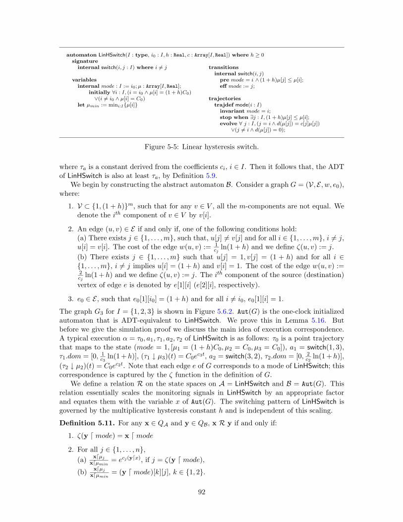
automaton LinHSwitch(I : type, i0 : I, h : Real, c : Array[I, Real]) where h ≥ 0signature
internal switch(i, j : I) where i 6= j
variablesinternal mode : I := i0;µ : Array[I, Real];
initially ∀i : I, (i = i0 ∧ µ[i] = (1 + h)C0)∨(i 6= i0 ∧ µ[i] = C0)
let µmin := mini:Iµ[i]
transitionsinternal switch(i, j)
pre mode = i ∧ (1 + h)µ[j] ≤ µ[i];eff mode := j;
trajectoriestrajdef mode(i : I)
invariant mode = i;stop when ∃j : I, (1 + h)µ[j] ≤ µ[i];evolve ∀ j : I, (j = i ∧ d(µ[j]) = c[j]µ[j])
∨(j 6= i ∧ d(µ[j]) = 0);
Figure 5-5: Linear hysteresis switch.
where τa is a constant derived from the coefficients ci, i ∈ I. Then it follows that, the ADTof LinHSwitch is also at least τa, by Definition 5.9.
We begin by constructing the abstract automaton B. Consider a graph G = (V, E , w, e0),where:
1. V ⊂ 1, (1 + h)m, such that for any v ∈ V , all the m-components are not equal. Wedenote the ith component of v ∈ V by v[i].
2. An edge (u, v) ∈ E if and only if, one of the following conditions hold:(a) There exists j ∈ 1, . . . ,m, such that, u[j] 6= v[j] and for all i ∈ 1, . . . ,m, i 6= j,u[i] = v[i]. The cost of the edge w(u, v) := 1
cjln(1 + h) and we define ζ(u, v) := j.
(b) There exists j ∈ 1, . . . ,m such that u[j] = 1, v[j] = (1 + h) and for all i ∈1, . . . ,m, i 6= j implies u[i] = (1 + h) and v[i] = 1. The cost of the edge w(u, v) :=2cj
ln(1 + h) and we define ζ(u, v) := j. The ith component of the source (destination)vertex of edge e is denoted by e[1][i] (e[2][i], respectively).
3. e0 ∈ E , such that e0[1][i0] = (1 + h) and for all i 6= i0, e0[1][i] = 1.
The graph G3 for I = 1, 2, 3 is shown in Figure 5.6.2. Aut(G) is the one-clock initializedautomaton that is ADT-equivalent to LinHSwitch. We prove this in Lemma 5.16. Butbefore we give the simulation proof we discuss the main idea of execution correspondence.A typical execution α = τ0, a1, τ1, a2, τ2 of LinHSwitch is as follows: τ0 is a point trajectorythat maps to the state (mode = 1, [µ1 = (1 + h)C0, µ2 = C0, µ3 = C0]), a1 = switch(1, 3),τ1.dom = [0, 1
c3ln(1 +h)], (τ1 ↓ µ3)(t) = C0e
c3t, a2 = switch(3, 2), τ2.dom = [0, 2c2
ln(1 +h)],(τ2 ↓ µ2)(t) = C0e
c2t. Note that each edge e of G corresponds to a mode of LinHSwitch; thiscorrespondence is captured by the ζ function in the definition of G.
We define a relation R on the state spaces on A = LinHSwitch and B = Aut(G). Thisrelation essentially scales the monitoring signals in LinHSwitch by an appropriate factorand equates them with the variable x of Aut(G). The switching pattern of LinHSwitch isgoverned by the multiplicative hysteresis constant h and is independent of this scaling.
Definition 5.11. For any x ∈ QA and y ∈ QB, x R y if and only if:
1. ζ(y d mode) = x d mode
2. For all j ∈ 1, . . . , n,(a) xdµj
xdµmin= ecj(ydx), if j = ζ(y d mode),
(b) xdµj
xdµmin= (y d mode)[k][j], k ∈ 1, 2.
92
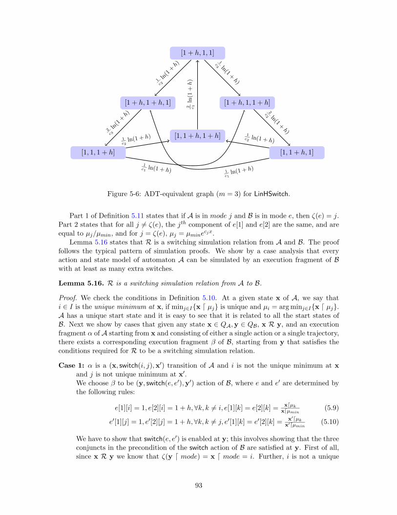
[1 + h, 1, 1]
[1 + h, 1 + h, 1] [1 + h, 1, 1 + h]
[1, 1, 1 + h] [1, 1 + h, 1]
[1, 1 + h, 1 + h]
1c 2
ln(1
+h)
1c3 ln(1
+h)
2c 3
ln(1
+h)
2c2 ln(1
+h)
1c2
ln(1 + h)
1c1
ln(1 + h)
1c2
ln(1 + h)
1c1
ln(1 + h)
2 c1
ln(1
+h)
Figure 5-6: ADT-equivalent graph (m = 3) for LinHSwitch.
Part 1 of Definition 5.11 states that if A is in mode j and B is in mode e, then ζ(e) = j.Part 2 states that for all j 6= ζ(e), the jth component of e[1] and e[2] are the same, and areequal to µj/µmin, and for j = ζ(e), µj = µmine
cjx.Lemma 5.16 states that R is a switching simulation relation from A and B. The proof
follows the typical pattern of simulation proofs. We show by a case analysis that everyaction and state model of automaton A can be simulated by an execution fragment of Bwith at least as many extra switches.
Lemma 5.16. R is a switching simulation relation from A to B.
Proof. We check the conditions in Definition 5.10. At a given state x of A, we say thati ∈ I is the unique minimum at x, if minj∈Ix d µj is unique and µi = arg minj∈Ix d µj.A has a unique start state and it is easy to see that it is related to all the start states ofB. Next we show by cases that given any state x ∈ QA,y ∈ QB, x R y, and an executionfragment α of A starting from x and consisting of either a single action or a single trajectory,there exists a corresponding execution fragment β of B, starting from y that satisfies theconditions required for R to be a switching simulation relation.
Case 1: α is a (x, switch(i, j),x′) transition of A and i is not the unique minimum at xand j is not unique minimum at x′.We choose β to be (y, switch(e, e′),y′) action of B, where e and e′ are determined bythe following rules:
e[1][i] = 1, e[2][i] = 1 + h,∀k, k 6= i, e[1][k] = e[2][k] = xdµk
xdµmin(5.9)
e′[1][j] = 1, e′[2][j] = 1 + h,∀k, k 6= j, e′[1][k] = e′[2][k] = x′dµk
x′dµmin(5.10)
We have to show that switch(e, e′) is enabled at y; this involves showing that the threeconjuncts in the precondition of the switch action of B are satisfied at y. First of all,since x R y we know that ζ(y d mode) = x d mode = i. Further, i is not a unique
93

minimum at x, so from the definition of the edges of G it follows that:
(y d mode)[1][i] = 1, (y d mode)[2][i] = i+ h,
∀k, k 6= i, (y d mode)[1][k] = (y d mode)[2][k] = xdµk
xdµmin(5.11)
Comparing Equations (5.11) and (5.17) we conclude that y d mode = e.
Secondly, using the definitions of e, e′ and R it follows that:
e[2][i] = 1 + h =x d µi
x d µmin=
x′ d µix′ d µmin
= e′[1][i] (5.12)
The second equality holds because switch(i, j) is enabled at x. The third equalityfollows from the fact that the switch(i, j) transition of A does not alter the value ofthe µk’s. Likewise, we have:
e[2][j] =x d µj
x d µmin=
x′ d µjx′ d µmin
= 1 = e′[1][j] (5.13)
∀k, k 6= j, k 6= i, e[2][k] =x d µk
x d µmin=
x′ d µkx′ d µmin
= e′[1][k] (5.14)
Combining Equations (5.12),(5.12) and (5.14) it follows that e[2] = e′[1].
Finally, from the switching simulation relation R, we know that y d x = 1ci
ln xdµi
xdµmin=
1ci
ln(1 + h). And since ζ(e) = i and i is not the unique minimum at x, from thedefinition of the edge costs of G it follows that y d x = w(e). Thus, we have shownthat switch(e, e′) is indeed enabled at y.
Next, we have to show that x′ R y′. First of all, x′ d mode = j and y′ d mode = e′
from the effect parts of the switch(i, j) and switch(e, e′) actions, respectively. Also,ζ(e′) = j from Equation (5.17). It follows that x′ d mode = ζ(y′ d mode). Secondly,x′dµj
x′dµmin= xdµj
xdµmin= 1, from the precondition of switch(i, j). Since y′ d x = 0 it follows
that xdµj
xdµmin= ecjy
′dx. Finally, for all k 6= j, again from Equation (5.17) it follows thatx′dµk
x′dµmin= e′[1][k] = e′[2][k].
Case 2: α is a (x, switch(i, j),x′) transition of A and i is the unique minimum at x and jis not unique minimum at x′.We choose β to be (y, switch(e, e′),y′) action of B, where e and e′ are determined bythe following rules:
e[1][i] = 1, e[2][i] = 1 + h,∀k, k 6= i, e[1][k] = (1 + h), e[2][k] = 1 (5.15)
e′[1][j] = 1, e′[2][j] = 1 + h,∀k, k 6= j, e′[1][k] = e′[2][k] = x′dµk
x′dµmin(5.16)
The rest of the proof is similar to that of case 1.
Case 3: α is a (x, switch(i, j),x′) transition of A and i is not the unique minimum at xand j is the unique minimum at x′.We choose β to be (y, switch(e, e′),y′) action of B, where e and e′ are determined by
94
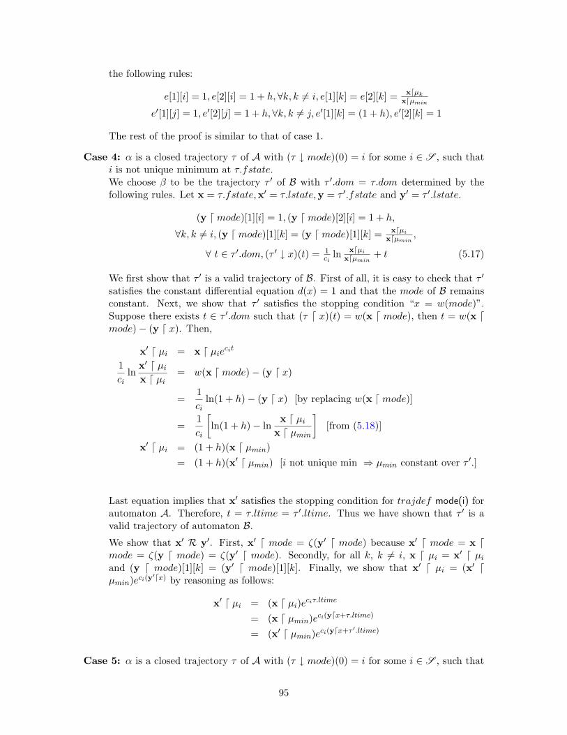
the following rules:
e[1][i] = 1, e[2][i] = 1 + h,∀k, k 6= i, e[1][k] = e[2][k] = xdµk
xdµmin
e′[1][j] = 1, e′[2][j] = 1 + h,∀k, k 6= j, e′[1][k] = (1 + h), e′[2][k] = 1
The rest of the proof is similar to that of case 1.
Case 4: α is a closed trajectory τ of A with (τ ↓ mode)(0) = i for some i ∈ S , such thati is not unique minimum at τ.fstate.We choose β to be the trajectory τ ′ of B with τ ′.dom = τ.dom determined by thefollowing rules. Let x = τ.fstate,x′ = τ.lstate,y = τ ′.fstate and y′ = τ ′.lstate.
(y d mode)[1][i] = 1, (y d mode)[2][i] = 1 + h,
∀k, k 6= i, (y d mode)[1][k] = (y d mode)[1][k] = xdµi
xdµmin,
∀ t ∈ τ ′.dom, (τ ′ ↓ x)(t) = 1ci
ln xdµi
xdµmin+ t (5.17)
We first show that τ ′ is a valid trajectory of B. First of all, it is easy to check that τ ′
satisfies the constant differential equation d(x) = 1 and that the mode of B remainsconstant. Next, we show that τ ′ satisfies the stopping condition “x = w(mode)”.Suppose there exists t ∈ τ ′.dom such that (τ d x)(t) = w(x d mode), then t = w(x dmode)− (y d x). Then,
x′ d µi = x d µiecit
1ci
lnx′ d µix d µi
= w(x d mode)− (y d x)
=1ci
ln(1 + h)− (y d x) [by replacing w(x d mode)]
=1ci
[ln(1 + h)− ln
x d µix d µmin
][from (5.18)]
x′ d µi = (1 + h)(x d µmin)= (1 + h)(x′ d µmin) [i not unique min ⇒ µmin constant over τ ′.]
Last equation implies that x′ satisfies the stopping condition for trajdef mode(i) forautomaton A. Therefore, t = τ.ltime = τ ′.ltime. Thus we have shown that τ ′ is avalid trajectory of automaton B.
We show that x′ R y′. First, x′ d mode = ζ(y′ d mode) because x′ d mode = x dmode = ζ(y d mode) = ζ(y′ d mode). Secondly, for all k, k 6= i, x d µi = x′ d µiand (y d mode)[1][k] = (y′ d mode)[1][k]. Finally, we show that x′ d µi = (x′ dµmin)eci(y
′dx) by reasoning as follows:
x′ d µi = (x d µi)eciτ.ltime
= (x d µmin)eci(ydx+τ.ltime)
= (x′ d µmin)eci(ydx+τ′.ltime)
Case 5: α is a closed trajectory τ of A with (τ ↓ mode)(0) = i for some i ∈ S , such that
95
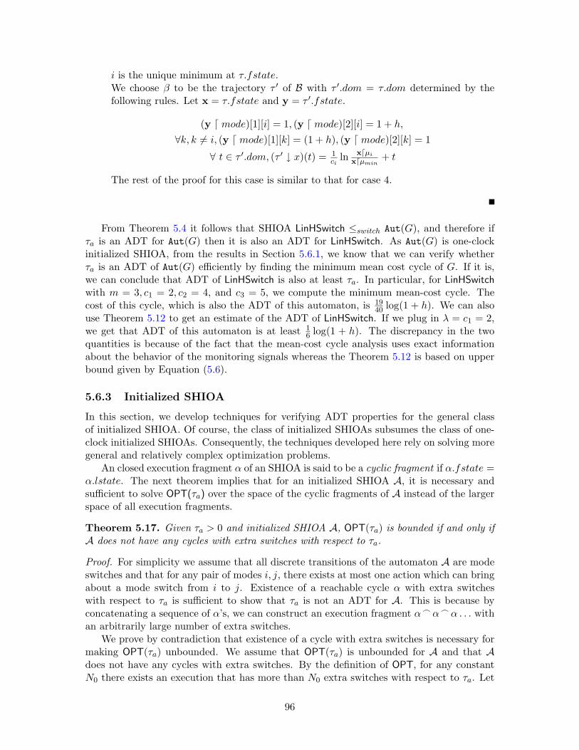
i is the unique minimum at τ.fstate.We choose β to be the trajectory τ ′ of B with τ ′.dom = τ.dom determined by thefollowing rules. Let x = τ.fstate and y = τ ′.fstate.
(y d mode)[1][i] = 1, (y d mode)[2][i] = 1 + h,
∀k, k 6= i, (y d mode)[1][k] = (1 + h), (y d mode)[2][k] = 1
∀ t ∈ τ ′.dom, (τ ′ ↓ x)(t) = 1ci
ln xdµi
xdµmin+ t
The rest of the proof for this case is similar to that for case 4.
From Theorem 5.4 it follows that SHIOA LinHSwitch ≤switch Aut(G), and therefore ifτa is an ADT for Aut(G) then it is also an ADT for LinHSwitch. As Aut(G) is one-clockinitialized SHIOA, from the results in Section 5.6.1, we know that we can verify whetherτa is an ADT of Aut(G) efficiently by finding the minimum mean cost cycle of G. If it is,we can conclude that ADT of LinHSwitch is also at least τa. In particular, for LinHSwitchwith m = 3, c1 = 2, c2 = 4, and c3 = 5, we compute the minimum mean-cost cycle. Thecost of this cycle, which is also the ADT of this automaton, is 19
40 log(1 + h). We can alsouse Theorem 5.12 to get an estimate of the ADT of LinHSwitch. If we plug in λ = c1 = 2,we get that ADT of this automaton is at least 1
6 log(1 + h). The discrepancy in the twoquantities is because of the fact that the mean-cost cycle analysis uses exact informationabout the behavior of the monitoring signals whereas the Theorem 5.12 is based on upperbound given by Equation (5.6).
5.6.3 Initialized SHIOA
In this section, we develop techniques for verifying ADT properties for the general classof initialized SHIOA. Of course, the class of initialized SHIOAs subsumes the class of one-clock initialized SHIOAs. Consequently, the techniques developed here rely on solving moregeneral and relatively complex optimization problems.
An closed execution fragment α of an SHIOA is said to be a cyclic fragment if α.fstate =α.lstate. The next theorem implies that for an initialized SHIOA A, it is necessary andsufficient to solve OPT(τa) over the space of the cyclic fragments of A instead of the largerspace of all execution fragments.
Theorem 5.17. Given τa > 0 and initialized SHIOA A, OPT(τa) is bounded if and only ifA does not have any cycles with extra switches with respect to τa.
Proof. For simplicity we assume that all discrete transitions of the automaton A are modeswitches and that for any pair of modes i, j, there exists at most one action which can bringabout a mode switch from i to j. Existence of a reachable cycle α with extra switcheswith respect to τa is sufficient to show that τa is not an ADT for A. This is because byconcatenating a sequence of α’s, we can construct an execution fragment α_ α_ α . . . withan arbitrarily large number of extra switches.
We prove by contradiction that existence of a cycle with extra switches is necessary formaking OPT(τa) unbounded. We assume that OPT(τa) is unbounded for A and that Adoes not have any cycles with extra switches. By the definition of OPT, for any constantN0 there exists an execution that has more than N0 extra switches with respect to τa. Let
96

us choose N0 > |I|3. Of all the executions that have more than N0 extra switches, letα = τ0a1τ1 . . . τn be a closed execution that has the smallest number of mode switches.From α, we construct β = τ∗0 a1τ
∗1 . . . τ
∗n, using the following two rules:
1. Each τi of α is replaced by: τ∗i = arg minτ.ltime | τ.fstate ∈ Rai , τ.lstate ∈ Preai+1.
2. If there exists i, j ∈ I, such that ai = aj and ai+1 = aj+1, then we make τ∗i = τ∗j .
Claim 5.18. The sequence β is an execution fragment of A and Sτa(β) > |I|3.
Proof of claim: We prove the first part of the claim by showing that each application of theabove rules to an execution fragment of A results in another execution fragment. ConsiderRule (1) and fix i. Since τ∗i .fstate ∈ Rai and τi−1.lstate ∈ Preai , τi−1.lstate
ai→ τ∗i .fstate.And, since τ∗i .lstate ∈ Preai+1 and τi+1.fstate ∈ Rai+1 , we know that τ∗i .lstate
ai+1→τi+1.fstate. Now for Rule (2), we assume there exist i and j such that the hypothesisof the rule holds and suppose τ∗j = τ∗i = τi. We know that even if τ∗j 6= τj , the first statesof both are in Raj and the last states are in Preaj+1 . Therefore, aj matches up the statesof τj−1 and τ∗j and likewise aj+1 matches the states of τ∗j and τj+1.
The second part of the claim follows from the fact that each trajectory τi is replaced bythe shortest trajectory τ∗i from the initialization set of the previous transition Rai to theguard set of the next transition Preai+1 . That is, for each i, 0 < i < n, τ∗i .ltime ≤ τi.ltime
and therefore β.ltime ≤ α.ltime and Sτa(β) > N0 > |I|3.
Since N(β) > |I|3, there must be a sequence of 3 consecutive modes that appear multipletimes in β. That is, there exist i, j ∈ 1, . . . ,m, and p, q, r ∈ I, such that τ∗i .fstate dmode = τ∗j .fstate d mode = p, τ∗i+1.fstate d mode = τ∗j+1.fstate d mode = q, andτ∗i+2.fstate d mode = τ∗j+2.fstate d mode = r. Then, from Rule (2) we know thatτ∗i+1 = τ∗j+1. In particular, τ∗i+1.fstate = τ∗j+1.fstate, that is, we can write β = βp
_ γ_ βs,where γ is a cycle. Then we have the following:
N(βp) +N(γ) +N(βs) > N0 + βp.ltime/τa + γ.ltime/τa + βs.ltime/τa
N(βp) +N(βs) + Sτa(γ) > N0 + βp.ltime/τa + βs.ltime/τa
N(βp_ βs) > N0 + βp
_ βs.ltime/τa [βp.lstate = βs.fstate]
The last step follows from the assumption that Sτa(γ) ≤ 0. Therefore, we have Sτa(βp _
βs) > N0 which contradicts our assumption that β has the smallest number of mode switchesamong all the executions that have more than N0 extra switches with respect to τa.
The following corollary allows us to limit the search for cycles with extra switches tocycles with at most |I|3 mode switches. It is proved by showing that any cycle with extraswitches that has more than |I|3 mode switches can be decomposed into two smaller cycles,one of which must also have extra switches.
Corollary 5.19. Suppose A is an initialized SHIOA with state models indexed by I. If Ahas a cycle with extra switches, then it has a cycle with extra switches that has fewer than|I|3 mode switches.
Theorem 5.20. Suppose A is an initialized SHIOA with state models indexed by I. Forany τa > 0, τa is an ADT for A if an only if all cycles of length at most |I| are free of extraswitches.
97

Proof. Follows from Corollary 5.19 and the definition of the optimization problem OPT(τa).
This theorem gives us a method for verifying ADT of initialized SHIOAs by maximizingOPT(τa) over all cycles of length at most |I|. In other words, for verify ADT of initializedhybrid systems it suffices to solve the optimization problem over a much smaller set ofexecutions than we set out with at the beginning of Section 5.6. For non-initialized SHIOAA, the first part of Theorem 5.17 holds. That is, solving OPT(τa) over all cycles of lengthat most |I|, if a cycle with extra switches is found, then we can conclude that τa is notan ADT for A. Solving OPT(τa) relies on formulating it as a mathematical program suchthat standard mathematical programming tools can be used. This is the topic of the nextsection.
5.6.4 MILP formulation of OPT(τa)
In this section, we show that the problem of solving OPT(τa) over the cyclic executions ofa rectangular SHIOA can be formulated as a Mixed Integer Linear Programming (MILP).Recall Definition 2.16, where we defined rectangular SHIOAs to have rectangular dynamicsand linier guards, invariants, and reset maps.
The Rectangular automaton (Figure 5-7) shows the specification of a generic initializedrectangular SHIOA with n continuous variables, n ∈ N, and m = |I| state models. Forthe sake of avoiding clutter, the code in this figure omits the following type informationfor the automaton parameters. (1) I is a type parameter which serves as the index setfor the state models. (2) i0 ∈ I is the index of the initial state model. (3) x0 is a real-valued n vector which serves as the initial valuation for the continuous variables. (4) Foreach i, j ∈ I, G[i, j], R[i, j], and A[i] are real-valued n × n matrices, (5) For each i, j ∈ I,g[i, j], r[i, j], a[i], and c[i] are real-valued n vectors. The automaton Rectangular has a singlediscrete variable called mode which takes values in the index set I = 1, . . . ,m, and acontinuous variable vector x ∈ Rn. For any i, j ∈ I, the switch(i, j) action changes modefrom i to j. The precondition and the initialization predicates of this action are given bysets of linear inequalities on the continuous variables, represented by: G[i, j]x ≤ g[i, j] andR[i, j]x ≤ r[i, j], respectively. For each state model i ∈ I, the invariant is stated in termsof linear inequalities of the continuous variables A[i]x ≤ a[i]. The evolve clause is given bya single differential equation d(x) = c[i].
automaton Rectangular(I, i0,x0, G, g,R, r, A, a, c)signature
internal switch(i, j : I), where i 6= j
variablesinternal mode : I := i;x : Rn := x0;
transitionsinternal switch(i, j)
pre mode = i ∧G[i, j]x ≤ g[i, j];eff mode := j; x := x′ where R[i, j]x′ ≤ r[i, j];
trajectoriestrajdef mode(i : I)invariant A[i]x ≤ a[i];evolve d(x) = c[i];
Figure 5-7: Generic rectangular initialized SHIOA.
We describe a MILP formulation MOPT(K, τa) for finding a cyclic execution with Kmode switches that maximizes the number of extra switches with respect to τa. If theoptimal value is positive, then the optimal solution represents a cycle with extra switches
98
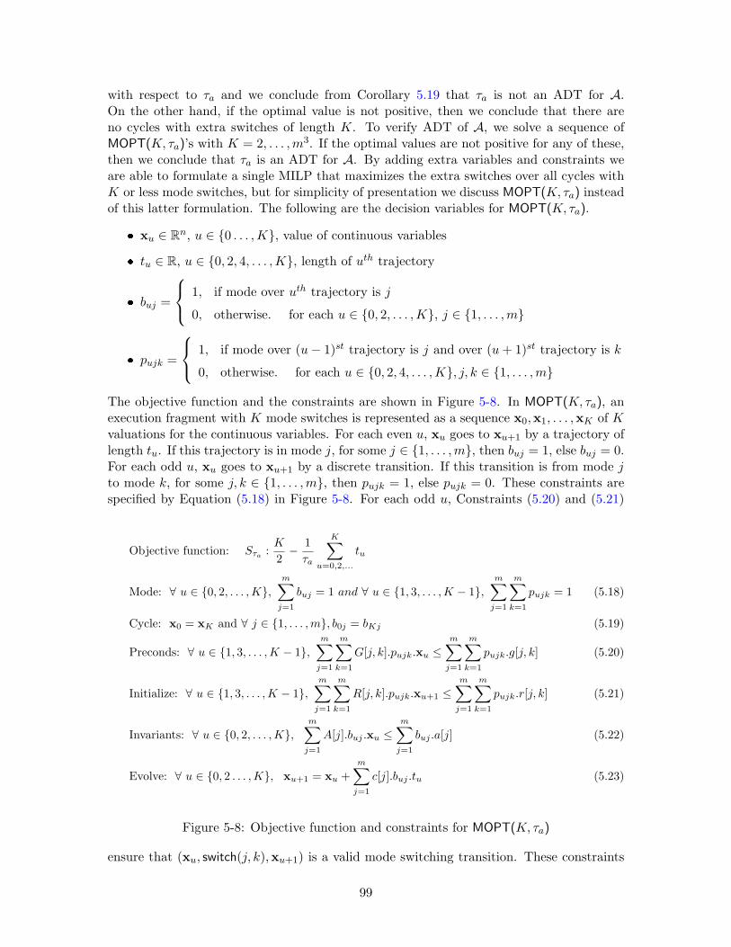
with respect to τa and we conclude from Corollary 5.19 that τa is not an ADT for A.On the other hand, if the optimal value is not positive, then we conclude that there areno cycles with extra switches of length K. To verify ADT of A, we solve a sequence ofMOPT(K, τa)’s with K = 2, . . . ,m3. If the optimal values are not positive for any of these,then we conclude that τa is an ADT for A. By adding extra variables and constraints weare able to formulate a single MILP that maximizes the extra switches over all cycles withK or less mode switches, but for simplicity of presentation we discuss MOPT(K, τa) insteadof this latter formulation. The following are the decision variables for MOPT(K, τa).
xu ∈ Rn, u ∈ 0 . . . ,K, value of continuous variables
tu ∈ R, u ∈ 0, 2, 4, . . . ,K, length of uth trajectory
buj =
1, if mode over uth trajectory is j
0, otherwise. for each u ∈ 0, 2, . . . ,K, j ∈ 1, . . . ,m
pujk =
1, if mode over (u− 1)st trajectory is j and over (u+ 1)st trajectory is k
0, otherwise. for each u ∈ 0, 2, 4, . . . ,K, j, k ∈ 1, . . . ,m
The objective function and the constraints are shown in Figure 5-8. In MOPT(K, τa), anexecution fragment with K mode switches is represented as a sequence x0,x1, . . . ,xK of Kvaluations for the continuous variables. For each even u, xu goes to xu+1 by a trajectory oflength tu. If this trajectory is in mode j, for some j ∈ 1, . . . ,m, then buj = 1, else buj = 0.For each odd u, xu goes to xu+1 by a discrete transition. If this transition is from mode jto mode k, for some j, k ∈ 1, . . . ,m, then pujk = 1, else pujk = 0. These constraints arespecified by Equation (5.18) in Figure 5-8. For each odd u, Constraints (5.20) and (5.21)
Objective function: Sτa:K
2− 1τa
K∑u=0,2,...
tu
Mode: ∀ u ∈ 0, 2, . . . ,K,m∑
j=1
buj = 1 and ∀ u ∈ 1, 3, . . . ,K − 1,m∑
j=1
m∑k=1
pujk = 1 (5.18)
Cycle: x0 = xK and ∀ j ∈ 1, . . . ,m, b0j = bKj (5.19)
Preconds: ∀ u ∈ 1, 3, . . . ,K − 1,m∑
j=1
m∑k=1
G[j, k].pujk.xu ≤m∑
j=1
m∑k=1
pujk.g[j, k] (5.20)
Initialize: ∀ u ∈ 1, 3, . . . ,K − 1,m∑
j=1
m∑k=1
R[j, k].pujk.xu+1 ≤m∑
j=1
m∑k=1
pujk.r[j, k] (5.21)
Invariants: ∀ u ∈ 0, 2, . . . ,K,m∑
j=1
A[j].buj .xu ≤m∑
j=1
buj .a[j] (5.22)
Evolve: ∀ u ∈ 0, 2 . . . ,K, xu+1 = xu +m∑
j=1
c[j].buj .tu (5.23)
Figure 5-8: Objective function and constraints for MOPT(K, τa)
ensure that (xu, switch(j, k),xu+1) is a valid mode switching transition. These constraints
99

simplify to the inequalities G[j, k]xu ≤ g[j, k] and R[j, k]xu+1 ≤ r[j, k] which correspondto the precondition and the initialization conditions on the pre and the post-state of thetransition. For each even u, xu evolves to xu+1 through a trajectory in some mode, sayj. Constraint (5.22) ensures that xu satisfies the invariant of mode j described by theinequality A[j]xu ≤ a[j]. An identical constraint for xu+1 is written by replacing xu withxu+1 in (5.22). Since the differential equations have constant right hand sides and theinvariants describe polyhedra in Rn, the above conditions ensure that all the intermediatestates in the trajectory satisfy the mode invariant. Equation (5.23) ensures that, for eacheven u, xu evolves to xu+1 in tu time according to the differential equation d(x) = c[j].
Some of these constrains involve nonlinear terms. Using the “big M” method [Wil90] wecan linearize these equation and inequalities. For example, bujxu in (5.22) is the product ofreal variable xu and boolean variable buj . We linearize it by replacing bujxu with yu, andadding the following linear inequalities: yu ≥ bujδ, yu ≤ buj∆, yu ≤ xu − (1 − buj)δ, andyu ≥ xu − (1− buj)∆, where δ and ∆ are the lower and upper bounds on the values of xu.
5.6.5 Case Study: Thermostat
We use the MILP technique together with switching simulation relations to verify the ADTof a thermostat with nondeterministic switches. The Thermostat2 automaton (Figure 5-9Left) has two modes on and off , two continuous variables x and z, and real parametersh,K, θ1, θ2, θ3, θ4, where 0 < θ1 < θ2 < θ3 < θ4 < h. In off mode the heater is off andthe temperature x decreases according to the differential equation d(x) = −Kx. This isdescribed by the state model heaterOff. While the temperature x is between θ2 and θ1,the switchOn action may occur, and it must occur when x drops to θ1. As an effect ofswitchOn, the mode changes to on, where the heater is on and the behavior is described bystate model heaterOn. Here, x rises according to the differential equation d(x) = K(h− x).While x is between θ3 and θ4, the switchOff action may occur, and it must occur when xincreases to θ4. The continuous variable z measures the total time spent in mode on.
SHIOA Thermostat2 is not initialized because the continuous variable x is not resetwith every mode switching transition; nor is it a rectangular SHIOA because the differen-tial equations do not have constant right-hand sides. There exists, however, a rectangularinitialized SHIOA, we call it ThermAbs, such that Thermostat2 ≤switch ThermAbs. Automa-ton ThermAbs (Figure 5-9 Right) has real-valued parameters L0 and L1, a clock variablet, and two modes on and off . In each mode, t increases at a unit rate. When t reachesLi in mode li, a switch to the other mode may occur and if it does then t is set to zero.We define a relation R on the state spaces of Thermostat2 and ThermAbs such that withappropriately chosen values of L0 and L1, ThermAbs captures the fastest switching behaviorof Thermostat2.
Definition 5.12. For any x ∈ QThermostat and y ∈ QThermAbs, x R y if and only if:
(1) x d mode = y d mode, and
(2) if x d mode = l0 then y d t ≥ 1k ln θ3
xdx else y d t ≥ 1k ln
(h−θ2h−xdx
).
Lemma 5.21. If we set L0 = 1k ln θ3
θ2and L1 = 1
k ln h−θ2h−θ3 , then the relation R of Defini-
tion 5.12 is a switching simulation relation from Thermostat2 to ThermAbs.
100

automaton Thermostat2(θ1, θ2, θ3, θ4,K, h : Real)where 0 < θ1 < θ2 < θ3 < θ4 < h
type Status enumeration [on, off ]
signatureinternal switchOn, switchOff
variablesinternal loc : Status := off ;x : Real := θ4; z : Real := 0;
transitionsinternal heaterOn
pre loc = off ∧x ≤ θ2;eff loc := on;
internal switchOffpre loc = on ∧x ≥ θ3;eff loc := off ;
trajectoriestrajdef heaterOn
invariant x ≤ θ4 ∧ loc = on;stop when x = θ4;evolve d(x) = K(h− x); d(z) = 1;
trajdef heaterOffinvariant x ≥ θ1 ∧ loc = off ;stop when x = θ1;evolve d(x) = −Kx; d(z) = 0;
automaton ThermAbs(L0, L1 : Real)type Status enumeration [on, off ]
signatureinternal switchOn, switchOff
variablesinternal mode : Status := off ; r : Real := L1;
transitionsinternal switchtOn
pre mode = off ∧ r ≥ L0;eff mode := on; r := 0;
internal switchOffpre mode = on ∧ r ≥ L1;eff mode := off ; r := 0;
trajectoriestrajdef alwaysevolve d(r) = 1;
Figure 5-9: Thermostat2 SHIOA and its rectangular initialized abstraction ThermAbs.
Proof. The proof is by induction on the length of an execution of Thermostat2 and isstructurally similar to the proof of Lemma 5.16. The base case follows immediately asthe start state of Thermostat2 is related to the start state of ThermAbs. Next, for theinductive step we show by cases that given any state x ∈ QThermostat,y ∈ QThermAbs, x R y,and an execution fragment α of Thermostat2 starting from x and consisting of either asingle action or a single trajectory, there exists a corresponding execution fragment β ofThermAbs, starting from y that satisfies the conditions required for R to be a switchingsimulation relation.
Case 1: α is a (x, on,x′) transition of Thermostat2.We choose β to be the (y, on,y′) transition of ThermAbs. First we show that the actionon is enabled at y′. Since x R y, we know that y d mode = x d mode = l0 and further,y d r ≥ 1
k ln θ3xdx . But we know that, x d x ≤ θ2 because the on action of Thermostat2
is enabled at x. It follows that y d r ≥ 1k ln θ3
θ2= L0, that is, the on action is enabled
at y. Next we show that vx′ R y′. Its immediate that x′ d mode = l1 = y′ d mode.From the transition definition of both the on actions, it follows that y′ d r = 0 andx′ d x = x d x ≤ θ2 and ln h−θ2
h−x′dx ≤ 0. Therefore, y′ d r ≤ 1K ln h−θ2
h−x′dx .
Case 2: α is a (x, off,x′) transition of Thermostat2.We choose β to be the (y, on,y′) transition of ThermAbs and the rest of the proof issimilar to that of case 1.
Case 3: α is a single trajectory τ of Thermostat2 such that (τ ↓ mode)(0) = l0. We choose
101

β to be a trajectory τ ′ of ThermAbs defined as follows:
∀ t ∈ τ ′.dom, (τ ′ ↓ mode)(t) = l0 and (τ ′ ↓ r)(t) = (τ ′ ↓ r)(0) + t
It follows immediately that τ ′ is a valid trajectory for ThermAbs because it satisfiesthe the differential equation d(r)) = 1 and the mode remains constant.
Case 4: α is a single trajectory τ of Thermostat2 such that (τ ↓ mode)(0) = l1. The prooffor this case is the same as that of the previous case.
Lemma 5.21 implies that Thermostat2 ≤switch ThermAbs, that is, for any τa > 0 ifτa is an ADT for ThermAbs then τa is also an ADT for Thermostat2. Since ThermAbs isrectangular and initialized, we can use the MILP technique to check any ADT property ofThermAbs.
We formulated the MOPT(K, τa) for automaton ThermAbs and used the GNU LinearProgramming Kit [GNU] to solve it. Solving for K = 4, L0 = 40, L1 = 15, and τa =25, 27, 28, we get optimal costs −0.4,−4.358E−13(≈ 0) and 0.071, respectively. We concludethat the ADT of ThermAbs is ≥ 25,≥ 27, and < 28. Since ThermAbs ≥switch Thermostat2,we conclude that the ADT of the thermostat is no less than 27.
For finding counterexample execution fragments for the proposed ADT properties, theMILP approach can be applied to non-initialized rectangular SHIOA as well. In suchapplications, the necessity part of Theorem 5.17 does not hold and therefore from thefailure to find a counterexample we cannot conclude that the automaton satisfies the ADTproperty in question.
5.7 Summary
Using results from the literature on switched systems, we find that stability verification ofSHIOAs can be decomposed into two independent tasks, namely, (a) finding the Lyapunovfunctions for the individual state models, and (b) verifying the appropriate average dwelltime property. Task (a) can be accomplished using existing techniques in systems theory.In this chapter we have presented two techniques for accomplishing task (b).
The first method transforms the given SHIOA by adding history variables, such that thetransformed automaton satisfies an invariant property if and only if the original automatonhas the ADT property. In order to prove the resulting invariant properties, we appeal tothe large body of tools available for proving invariants for hybrid systems. This methodfor verifying ADT properties is automatic only for classes of hybrid systems for whichreachability is decidable. For hybrid systems that are outside this class, the method isapplicable, but the resulting invariants will have to be proved using the methods describedin Chapter 4 of this thesis.
The second method relies on solving an optimization problem over the set of cyclicexecutions of the given SHIOA. For the class of one-clock initialized SHIOAs this involvesfinding the maximum mean-cost cycle of a graph (of size comparable to the given SHIOA),and can be solved very efficiently by classical graph algorithms. For rectangular initializedSHIOAs, the optimization problem can be formulated as a MILP. For initialized SHIOAswith more general dynamics, the same technique applies but harder optimization problemswill have to be solved.
102

For non-initialized hybrid automata, the solution of the optimization problem can giveexecutions that serve as counterexamples to the ADT property in question, but the failurein finding such executions does not indicate that the ADT property in question is satisfied.That is, for non-initialized SHIOAs, the method is incomplete. We have defined equiva-lence of SHIOAs with respect to switching speed and proposed switching simulations forestablishing ADT-equivalence of two SHIOAs. This can serve as a method for abstractingnon-initialized SHIOAs with initialized ones.
The two methods for verifying ADT can be combined as follows: we can start with somecandidate value of τa > 0 and search for a counterexample execution fragment for it usingthe optimization-based approach. If such an execution fragment is found, then we decreaseτa (say, by a factor of 2) and try again. If eventually the optimization approach fails to finda counterexample execution fragment for a particular value of τa, then we use the invariantapproach to try to prove that this value of τa is an ADT for the given system.
There are several research directions to be pursued related to the general area of stabil-ity verification of SHIOAs. One interesting problem is to develop stability verificationtechniques for the general class of SHIOAs that have both stable and unstable state mod-els. Sufficient conditions for stability of such systems already exist in the control theoryliterature (see, for example [ZHYM00]). These conditions, however, take the form of switch-ing time related properties and are hard to verify, just like the ADT property, and hencethey call for the development of new verification techniques. Another direction, is to relaxassumption (1) and explore verification of input-output and input-to-state stability proper-ties of SHIOAs with input/output variables, using the results from [VCL06]. Yet anotherdirection of future research is to extend these techniques to stochastic hybrid systems, bycombining the probabilistic timed I/O automata of Chapter 7 with ADT-like stability re-sults for stochastic switched systems from [CL06].
103
Chapter 6
Mechanizing Proofs
In this chapter we describe techniques for mechanizing invariance and implementation proofsfor SHIOAs. The examples of Chapters 4 and 5 illustrate that the SHIOA frameworkprovides a systematic way of constructing such proofs, by way of induction over the lengthof the executions followed by case analysis of the actions and the state models. Often,however, such proofs are lengthy, tedious to construct, and they always require carefulattention to specification details. This suggests that software tools for construction andmanagement of proofs are needed.
Mechanical theorem provers, such as, PVS [ORR+96], Isabelle/HOL [Pau93, GCMF93],COQ [The04], provide their own specification languages, typically some variant of high-order logic, and very general semi-decision procedures for interactively checking veracityof formulae written in that language. In order to use a theorem prover for constructionand management of SHIOA proofs, we have to answer two questions: (a) translate HIOAspecifications to the language of the theorem prover, and (b) minimize interaction of theuser with the theorem prover. In Section 6.2, we address (a) by describing a scheme fortranslating a large class of HIOA specifications to the language of the PVS theorem prover.This work builds on and generalizes previous work on translating of Timed I/O Automatonspecifications to PVS [LKLM05]. In Section 6.3, we address (b) by describing a set of spe-cialized proof strategies—programs for constructing proofs—that exploit the knowledge ofour translation scheme and partially automate proofs. This section is based on a sequence ofpapers on strategy development [MA03, MA04, MA05, ALL+06]. We conclude the chapterby discussing our experiences in developing and using these software tools.
6.1 An Overview
PVS [ORR+96] is an environment for formal specification and verification developed at SRI.It consists of a specification language (henceforth PVS), a number of predefined theories,a type checker, an interactive theorem prover that supports the use of several decisionprocedures and a symbolic model checker. By exploiting the synergy between a highlyexpressive specification language and powerful automated deduction routines, PVS servesas an environment for constructing and maintaining large formalizations and proofs. Ourpreference of PVS over other existing theorem provers is based on several of its features:
(a) The PVS language [OSRSC99] is expressive, natural, and syntactically close to classi-cal, typed high-order logic. It has many attractive features including parameterizedspecifications and predicate subtyping.
104

(b) Theory interpretations [OS01], a new feature in PVS, is used to instantiate the declaredtypes in a specifications with definitions. Theory interpretations can be used for ex-hibiting models for an axiomatic theory and to refine a abstract specifications in termsof a concrete one. This feature is useful for defining simulation relations between a pairof SHIOAs (see Section 6.2.9).
(c) The PVS theorem prover [SORSC99] provides a set of powerful decision procedures.New state-of-the-art techniques are continually added to make the decision proceduresefficient. And with the excellent tutorials available [COR+95], this prover sports arelatively flatter learning curve.
(d) PVS provides a way of developing strategies [AVM03] for partially automating proofs.A proof strategy or a strategy is a Lisp program that accesses the state of an ongo-ing proof, constructs a sequence of proof steps on-the-fly, and applies it to the proof.Our techniques for partially automating proof construction are embodied by a set ofstrategies.
(e) PVS has been widely used in many verification projects throughout the world and hasa lively user community [ORSSC98, Int06]. The current version of PVS is open source(under the GPL license).
An alternative to translating HIOA specifications to PVS is to write this SHIOA specificationdirectly in PVS . The resulting PVS specification will be a set of definitions for the variables,actions, transitions, and trajectories, and a set of axioms defining the semantics of theseobjects. We have decided not to opt for this direct route for the following reasons: (a) HIOAhas the variables, transitions, and state model structure, which is a natural representation ofSHIOAs, (b) HIOA allows us to describe the transitions using operational semantics, whereasin PVS , transition definitions have to be functions or relations, (c) HIOA provides a naturalway for describing trajectories using differential equations, and (d) having the theorem-prover-independent HIOA language allows one to combine use of different tools designed forthe SHIOA framework. Hence, SHIOA specifications are written in the HIOA language, theseare translated to PVS , and then the PVS theorem prover is invoked on the translated PVSspecification.
There has been several prior proposals for translating certain subsets of the IOA language []to theorem provers, such as, Larch [BGL02, GG91], PVS [Dev99], and Isabelle [NW03,Pau93].
Our design of the HIOA to PVS translator builds upon [BGL02] and [Mit01], but the firstto translate the continuous aspects of the behavior of hybrid systems to the language of atheorem prover. The key insight gained from the previous works is to convert nondetermin-istic transition (and consequently trajectory) definitions into deterministic functions (of thepre-state) by adding extra parameters. This enables the theorem prover to compute thepost-state of a transition (or a trajectory) and simplifies theorem proving. This procedureof “determinizing” is further discussed in Section 6.2.6.
In the PVS parlance, definition of types, operators, lemmas, etc., constitute a theory .The Timed Automata Modeling Environment (TAME) of [Arc01] provides a PVS theorytemplate for describing a special kind of automata called MMT Automata (see Section 1.4or [MMT91] for details). One manually instantiates this theory template with the states,actions, and transitions of an MMT automaton, say A, to obtain the PVS theory that spec-ifies A. Instantiating a theory template is also the mechanism underlying our translation
105
scheme, although our theory template is closer to the one in [LKLM05]. The key differ-ence between the TAME-template and the template [LKLM05] has to do with how timeis modeled in the underlying mathematical models. In a timed I/O automaton, the modelof [LKLM05], progress of time and continuous evolution of variables are modeled by trajec-tories (as in SHIOAs). MMT-automata, on the other hand, do not have general continuousvariables; there are upper and lower time bounds associated with actions, and actions mustoccur within those time-bounds. Hence, in the template of [Arc01], advancement of t unitsof time is modeled by the occurrence of an action ν(t). The time-bounds for the actionsare enforced by deadline variables that enable the ν(t) action only when t amount of timecan elapse without violating those bounds. This approach does not allow us to specify in-teresting trajectories by asserting of properties that must hold throughout the duration of atrajectory . In [LKLM05] we proposed a template that allows translation of such trajectoriesby embedding the trajectory τ as a functional parameter of ν(t, τ). The enabling conditionof ν(t, τ) asserts the conditions that must hold at each point in the domain of τ . For exam-ple, we can say that a particular ν(τ, t) action is enabled only when τ.ltime < ubound andτ(t) d x = τ(0) d x+ 4t. Here, ubound is a discrete deadline variable and x is a continuousvariable increasing at four times the rate of real time.
The above translation scheme has been used to design the software tool for translat-ing TIOA specifications to PVS . This tool has been implemented by Lim [Lim01]. Recall,that the TIOA language is a restriction of HIOA which does not allow input/output vari-ables. In Section 6.2, we present the design of a scheme that generalizes the theory templateof [LKLM05] and allows translation of a general class of HIOA specification to PVS . Althoughthe basic mechanism for translation remains the same, namely, instantiation of templatetheories, several changes have been made in the templates to accommodate external vari-ables.
The possibility of partially automating proofs by using an interactive theorem prover wasdemonstrated earlier by the TAME system [Arc01] in the context of the MMT automatonmodel. TAME strategies primarily support proofs of invariant properties. These strategiesare compatible with the translation scheme described here and we describe them briefly inSection 6.3.1. Apart from partial automation, the TAME strategies illustrate that theoremprover support is useful for (a) managing large proofs, (b) re-checking proofs after minorchanges in the specification, and (c) generating human readable proofs from proof scripts.These strategies demonstrate how careful design of theory templates aid the developmentof proof strategies. Much of our later work [MA03, MA04, MA05, ALL+06] on developingproof strategies for implementation relations are informed by the lessons learned from theTAME experience. The technical challenges we faced during the development of these newstrategies are discussed in Section 6.2.9.
We have applied the translator and the strategies in several case studies: a tree-basedleader election protocol [MA04, MA05], Fischer’s mutual exclusion algorithm [ALL+06],a two-task race system, and a failure detector [LKLM05]. In Chapters 4 and 5 we haveshown how simulation relations are used for proving implementation and ADT-equivalenceof SHIOAs. A specific type of implementation that occurs quite often in real-time systemsinvolves showing that the actions of a given SHIOA A occur within certain time bounds.The bounds themselves may be complex functions of the parameters of A or dependenton external inputs. Such timing properties can be cast as implementation relations: firstan abstract SHIOA B is specified that has exactly the required timing behavior—this iseasy because we know the timing requirements that we wish to prove. Then, we show thatthat A implements B. In two of our case studies (Sections 6.4.1 and 6.4.2), we follow this
106

recipe and prove timing properties using simulation relations. In constructing the simulationproofs the strategies we have developed prove to be effective. In addition, the strategiesfor manipulation of real-inequalities provided by the Field [MM01] and the Manip [Vit02]packages are useful because these simulation relations involve inequalities between variablesof the system and its abstraction. Overall, our experience with the tool suggests thatit is possible (but not routine) to express realistic systems in HIOA , translate the HIOAspecification to PVS , and then prove properties of the system using PVS on the translatoroutput.
6.2 Translation
In this section we describe the design of a scheme for translating HIOA specifications toPVS . A HIOA specification file called say, xyz.hioa, when translated, produces a set ofPVS files containing several PVS theories. A summary of these files and their contentsare shown in Table 6.1. Essentially these generated theories contain definitions specifyingthe variables, actions, transitions, trajectories, and putative invariant predicates of theinput HIOA specification. Some theories such as xyz invariant and xyz 2 XYZ also containlemmas and theorems asserting properties such as invariance of predicates and simulationrelations. For generating these theories, the translator instantiates a PVS theory-templatewith the specifics obtained from xyz.hioa. These generated theories by themselves are notcomplete; they import a set of generic SHIOA library theories, that we have developed, fordefining the semantics of SHIOAs. One library theory, for example, defines what it means fora state of any SHIOA to be reachable in terms of abstract transitions and trajectories. Thecombination of the translated theories and the generic library theories completely describethe behavior of the particular SHIOA in question, and the PVS prover can be invoked toprove theorems about its behavior. In what follows, we take a closer look at the translation
Filename Theory name Description
xyz decls.pvs xyz Definition of the components of automaton xyz
common decls.pvs common decls Automaton parameters and where clause
xyz invariants.pvs xyz invariants Lemmas asserting invariants of xyz
xyz 2 XYZ.pvs xyz 2 XYZ Lemma asserting simulation from xyz to XYZ
Table 6.1: PVS files generated by translator.
of HIOA specifications to PVS theories and the definitions provided by the generic SHIOAlibrary theories.
6.2.1 Assumptions
The correct translation to PVS assumes the following two restrictions on the SHIOA A thatis specified in HIOA :
(1) A does not have input variables. In specifying A in PVS , we have to define its trajec-tories. Trajectories of input variables are restricted only by their dynamic types. Forspecifying dynamic types of continuous input variables we have to define the class of
107
functions that is piece-wise continuous. This poses certain difficulties because the the-ory of real analysis including continuity is not completely developed in PVS. Of course,when such a theory becomes available we can relax this assumption.
(2) HIOA allows us to define transitions of A by writing arbitrary relations relating the pre-and post-states. This is not allowed. The restriction allows us to convert transitionrelations to transition functions; thus we can compute the post state of a transition (ora trajectory) from its pre-state. Note that transitions (and trajectories) of A can stillhave nondeterminism through choose statements (and inequalities).
It is worth noting that HIOA specifications allow us to write arbitrarily complicated differ-ential equations in the state models. But, we cannot assert conditions involving derivativesand integrals of functions directly in PVS (see Section 6.2.7 for details). Hence, our trans-lation of state models relies on actually solving these differential equations, and therefore,we cannot automatically translate arbitrarily complex differential equations. In fact, thecurrent implementation of the TIOA to PVS translator can only translate specifications withstate models that have differential equations constant right hand sides. This is not a re-striction imposed by the translation scheme, but it reflects the limited ability of our currenttranslator software in solving differential equations. For classes of differential equationsoutside the above, solutions may be provided manually by the user. In the future, this stepcould also be automated by invoking external DAE solving tools such as Maple [GGC81]and Macsyma [Mat74].
6.2.2 Types and Vocabularies
Simple static types of HIOA , such as, Bool, Char, Int, Nat, Real, and String have theirequivalents in PVS. The HIOA types defined using the type constructors Enumeration,Tuple, Union, Set, Map, and Array are directly translated to type declarations in PVS . Thetype AugmentedReal is translated to a type called time which is defined as a Datatypethat is the union of two subtypes: non-negative reals (nnreal in PVS ) and a singleton typewith an element called infinity .
HIOA vocabularies are directly translated to PVS theories. The semantics of these typeand operator declarations are written in PVS library theories, which are imported by thetranslator output.
Example 6.1. The directedGraph vocabulary of Figure 3-2 is reproduced in Figure 6-1 along-side its PVS translation. The directedGraph theory is parameterized by the type parameterT . The sequences theory is a PVS library theory for finite sequences. The result of import-ing the sequences with parameter T into directedGraph is that the type sequence becomesdefined as a finite sequence of elements of type T , and the usual operators on objects oftype sequence become available in directedGraph. Tuples with accessors for the individualcomponents are called records in PVS and they are declared with [# . . .#] syntax. By im-porting directedGraph[I] into another PVS theory, directed graphs with vertices of type Ican be used. Notice that PVS allows us to declare connected as an abstract (uninterpreted)function. This is is sufficient to use it in other specifications, however, if we are inter-ested in proving theorems about a specification that relies on the behavior of connected,then we have two options: (1) We write axioms describing the of connected, for example,connected(a, b) ∧ connected(b, c) ⇒ connected(a, c). (2) We provide a concrete definitionfor computing connected; in this case, this would be an inductive definition.
108

vocabulary directedGraphs(T :type)typesEdge = Tuple [src : T, dst : T ];Digraph =
Tuple [vset :Set[T ], eset :Set[Edge]];Path = Seq [T ];
operatorsconnected : T, T → Bool;addEdge : Digraph,Edge→ Digraph;
end
directedGraphs[T: Type ]:TheoryBegin
Importing sequences[T ]
Edge: Type = [# src: T, dst:T # ]Digraph: Type =
[# vset: setof[T ], eset:setof[Edge ] # ]Path: Type = sequence
connected:[T,T → bool ]addEdge: [Digraph, Edge → Digraph ]
End directedGraphs
Figure 6-1: directedGraphs vocabulary in HIOA translated to directedGraphs theory in PVS.
Automaton parameters in HIOA are declared as constants in a separate PVS theory calledcommon decls. The where clause relating the automaton parameters is stated as an axiomrelating the constants.
6.2.3 Variables and Initial States
The set of valuations of output and internal variables of an SHIOA A are translated to twoseparate records types in PVS . A collection of output variables y1, y2, . . . , yn, of respectivetypes Y1, Y2, . . . , Yn, is translated to a record type declaration called OutputVals:
OutputVals: Type = [# y1:Y1, y2:Y2, · · ·, yn:Yn # ]
The type OutputVals corresponds to the set of all valuations of the output variables of A.The internal variable declarations are translated to similar record types called States. TheExternalVals, LocalVals, and Vals types, corresponding to the valuations of all the externalvariables, all the local variables, and all the variables of A, are defined as:
ExternalVals: Type = [# output: OutputVals # ]LocalVals: Type = [# states: States, output: OutputVals # ]Vals: Type = [# states: States, output: OutputVals # ].
There are two overlapping mechanisms for specifying the starting states of a SHIOAin the HIOA language: (a) individual variables are assigned particular values and (b) anpredicate on the variables defines the set of possible starting valuations. Both these featuresof HIOA are translated to a single predicate called Start in PVS.
Example 6.2. The HIOA code fragment from Section 3.2.4 and its PVS translation is shownin Figure 6-2. In translating variable types to PVS , the DiscreteReal variables are treatedin the same way as Real variables; additional constrains on the former variables appearwhen their trajectories are defined (see Section 6.2.7). Since initial values can be definedonly for internal variables in HIOA , Start is predicate on States and not Vals.
6.2.4 Trajectory Types
The PVS translation defines the following trajectory types derived from the variables types.These types are used in the subsequent definition of actions, transitions, and trajectories.
interval(t:nnreal):Type = t1:nnreal |t1 ≤ tTrajs(t:nnreal):Type = [interval(t) → Vals ]ExtTrajs(t:nnreal):Type = [interval(t) → ExternalVars ]
109

variablesoutput u : Discrete Real
internal x : Real := 5,y : Real := choose k where −5 ≤ k ≤ 5,z : Realinitially z × z + y × y ≤ 10
OutputVals: Type = [# u:real # ]States: Type = [# x:real, y:real, z:real # ]ExternalVals: Type = [# output:OutputVals # ]LocalVals: Type =
[# states:States, output:OutputVals # ]Vals: Type =
[# states:States, output:OutputVals # ]
Start(s:States): bool =x(s) = 5 Andy(s) ≥ -5 And y(s) ≤ 5 Andexp(z(s),2) + exp(y(s),2) ≤ 10
Figure 6-2: Variable declarations in HIOA translated to type declarations in PVS .
StateTrajs(t:nnreal):Type = [interval(t) → States ]
The type interval(t), for a non-negative real t, equals the real interval [0, t]. The typeTrajs(t) equals the set of functions that map the interval [0, t] to Vals, that is, valuationsof all the variables of A. Here we remark that the PVS type Trajs does not necessarilycorrespond to the mathematical object trajs(V ), where V is the set of variables of theautomaton being specified. The set trajs(V ) is the set of trajectories that respect thedynamics types of the individual variables in V . These functions in Trajs do not necessarilybelong to the dynamic types; dynamic type constraints cannot be stated in PVS at present.
The type ExtTrajs(t) equals the set of functions that map the interval [0, t] to ExternalVals,that is, valuations of the external variables of A. The parameterized types StateTrajs(t) isdefined analogously.
6.2.5 Actions, State Models, and Moves
The set of action names and state model names of an SHIOA are translated to a single PVSdatatype called Moves. Although actions and state models describe very different kindsof objects, they both define how the variables of an SHIOA changes, and at a syntacticlevel they play similar roles in defining the reachable states and traces of an SHIOA. Thus,putting them together in a common type simplifies the PVS theory. Informally, the Movesdatatype defines the names of all the possible ways in which the variables of the SHIOAA can change. For each action of A, Moves datatype has a separate constructor; andall the state models of A, are encapsulated by a single constructor called smodels. Theparameters of smodels constructor are explained in the following example. If an actionsand state models have formal parameters, the corresponding constructors have additionalparameters.
Four predicates are defined on Moves to distinguish the actions from the state models,and to distinguish the different kinds of actions from one another. For example, (Actions)is a subtype of Moves also (Trajectories) is a subtype of Moves. The following exampleillustrates these definitions.
Example 6.3. The PVS code fragment in Figure 6-3 shows the definition of the Movesdatatype for the Supervisor automaton from Chapter 4 (Figure 4-7). The enumerationtype SModelNames is derived from the names of the state models in the HIOA code, that is,the identifiers following the trajdef keyword. In PVS , a datatype is declared by giving alist of constructors-recognizers pairs. A datatype constructor is a function that returns anobject of the type that is being defined. And a recognizer returns true when it is applied to
110

an object that has been constructed using its constructor. For example, the second entryin the list for the Moves datatype is the constructor sample with parameters x0, x1, andits recognizer sample?. Hence, sample(π4 , 5) has type Moves. And for any object a of typeMoves, sample?(a) returns true if and only if a has been constructed using the sampleconstructor.
automaton Supervisor(umin, umax : Real)type
Mode = Enumeration [sup, usr ]
signatureinput sample(x0, x1 : Real)input usrOutput(u′ : Real)output supOutput(u′ : Real)
trajectoriestrajdef supMode. . .
trajdef usrMode. . .
SModelNames:Type = supMode, usrMode
Moves: Datatype Beginsmodel(name:Modes,
ltime:nnreal, tau:Trajs(ltime)):smodel?sample(x0, x1:real):sample?usrOutput(u:real):usrOutput?supOutput(u:real):supOutput?
End
Trajectories(a:Moves):bool = smodel?(a)Actions(a:Moves):bool = Not smodel?(a)InternalActions(a:(Actions)):bool = trueExternalActions(a:(Actions)):bool = false
Figure 6-3: Actions and State models in HIOA translated to Moves in PVS .
Each object defined by the smodel constructor corresponds to a trajectory of the vari-ables of A. The smodel constructor has three parameters: (1) name is the name of thestate model that defines the trajectory, (2) ltime is the limit time of the trajectory, and (3)tau is the trajectory itself.
The Trajectories predicate distinguish the Moves that correspond to smodel and fromthe others, namely those corresponding to actions. In PVS , a predicate p on a type T readilydefines a predicate subtype (p) ∆= x : T | p(a). In the above example, the (Actions)subtype is used to define the predicates the InternalActions and ExternalActions.
6.2.6 Transitions
Discrete transitions in HIOA are specified using preconditions and effects, and the state mod-els are specified using invariants, stopping conditions, and evolve-clauses. The PVS trans-lation of a HIOA specification converts these definitions into two independent definitions,namely, Enabled(m : Moves, v0 : Vals) : bool, and Trans(m : Moves, v0 : States) : Vals.The predicate Enabled(m, v0) returns true if and only if the move m is allowed at fromvaluation v0. The function Trans(m, v0) returns the valuations of the variables that resultfrom the occurrence of m at v0.
A couple of points are to be noted before we proceed to describe further details of thetranslation. First, in an execution of A, Trans(m, v0) is applicable for a given valuation v0and a given move m, only if Enabled(m, v0) is in fact true. This information, however, isnot available in the definition of Trans(m, v0) and hence in some cases the PVS type checkerproduces additional proof obligations called Type Correctness Conditions (TCCs). Forexample, consider a receive action that is Enabled when a queue is non-empty, and when theaction occurs it removes the first element of the queue. In type-checking the Trans functionfor receive, PVS will generate a TCC asserting the non-emptiness of queue (because thefirst element can be removed only for non-empty queues). This TCC can only be proved ifwe add the precondition of receive as a conditional in the eff program. Secondly, in HIOA
111

the valuations of the variables that result from the occurrence of a move (transition ortrajectory) may be chosen non-deterministically, however, Trans(m, v0) is a function whichuniquely determines the valuations. The missing step here is to introduce additional formalparameter(s) for such nondeterministic moves, whereby the choice of the values for theparameter(s) uniquely determine the valuation of the variables. This technique of pushinginternal nondeterminism (choices within a transition definition) to external nondeterminism(choice over several transitions) has been employed previously in [BGL02] and [Mit01] forthe purpose of transforming transition relations to transition functions. In this section wedescribe the translation of the discrete transitions and in Section 6.2.7 we describe thetranslation of the state models.
The Enabled predicate for actions is defined using a Case statement which contains thepreconditions from the HIOA specification. The HIOA program specifying the effects of tran-sitions consists of three types of sequential statements, namely, assignments, conditionals,and loops. Each of these statements is translated to its corresponding functional relationbetween states, as shown in Table 6.2.6. The term P is a HIOA program, while transP (v0)is a PVS function that returns the valuation obtained by performing program P on v0.Sequential statements like P1;P2 are translated to a composition of the corresponding func-
Statement type HIOA program P PVS translation transP (v)
Assignment x := exp v With [x := exp]
Conditional if pred then P1 fi If pred Then transP1 (v) Else v Endif
Conditional if pred then P1 else P2 fi If pred Then transP1 (v) Else transP2 (v) Endif
Loop for x in A do P1 od f orloop(A, v) : Recursive Vals =
If empty?(A) Then v Else v = choose(A),
s′ = f orloop(remove(x,A), v) In transP1 (v′) Endif
Measure card(A)
Table 6.2: Translation of program statements. v is a valuation of variables; exp is anexpression of type type(v); pred is a predicate; A is a finite set; choose picks an elementfrom A. WITH makes a copy of the record s, assigning the field v with a new value t.
tions transP2(transP1(v)). The translator can performs composition using the Let keywordof PVS for writing complex expressions through recursive substitutions. The program P1;
P2 can be written as LET v = transP1(v) IN transP2(v).
Example 6.4. Figure 6-4 shows an example that illustrates translation of assignments andconditionals. The effect of the foo transition is a set of arithmetic operations on the statevariables x and y. And the effect of bar swaps x and y if they are not equal. The PVStranslation is shown in the right column of Figure 6-4. In the transition of bar , x and y areassigned new values only when their values are not equal in the pre-state. Otherwise, theyare assigned their previous values.
In [LKLM05, Lim01], an alternative translation method using explicit substitutions isproposed. This approach explicitly specifies the resulting value of each variable in the post-state in terms of the variables in the pre-state [BGL02]. In the substitution method, thetranslator does the work of expressing the final value of a variable in terms of the values ofthe variables in the pre-state. In the LET method, the prover has to perform these sub-stitutions to obtain an expression for the post-state in an interactive proof. Therefore, thesubstitution method is more efficient for theorem proving, whereas the LET method pre-
112

transitionsinternal foo(i : Nat)
pre . . .eff x := x+ i; y := x× x;x := x− 1; y := y + 1;
internal barpre . . .eff t := x;
if x 6= ythen x := y;else y := t;
fi;
trans(m: Moves, v:Vals):Vals =Cases m Of
foo(i): v With [states :=(Let s: States = states(v) With [x := x(v) + i ] In(Let s: States = states(v) With [y := x(v) × x(v) ] In(Let s: States = states(v) With [x := x(v) -1 ] In(Let s: States = states(v) With [y := y(v) + 1 ] In s)))) ]
bar: v With [states :=(Let s: States = states(v) With [t := x(v) ] In(Let s: States =
If x(v) 6= q y(v) Then(Let s: States = states(v) With [x := y(v) ] In(Let s: States = states(v) With [y := t(v) ] In s))
Else s)) ]. . .
Endcases
Figure 6-4: Discrete transitions in HIOA and their PVS translation.
serves the sequential structure of the program, which is lost with the substitution method.Since the style of translation in some cases may be a matter of preference, we currentlysupport both approaches as an option for the user.
6.2.7 Trajectories
Recall from Section 6.2.5, that the names of the state models of SHIOAA are declared by thesmodel constructor in the Moves datatype. Each object of type Moves that is constructedby smodel corresponds to a trajectory of the variables of A and has three parameters: (1)name: the name of the state model, (2) ltime: the length of the trajectory, and (3) tau:the trajectory itself. The set of all possible trajectories of the variables of A is defined asthe type Trajs. Of all these trajectories, those that are actually permitted by A—as definedby its state model invariants, stopping conditions, and the evolve clauses—are specified bythe enabling condition of the corresponding move. Given a valuation v0 of type Vals andan object m of type Moves constructed using smodel, Enabled(m, v0) returns true only iftau(m) is a trajectory of A defined by the state model name(m) such that the startingvaluation of τ(m) is v0. Hence, Enabled(m, v0) encodes the conditions imposed by theinvariant, the stopping condition, and the evolve clause of the state model name(m). Andthe Trans(m, v0) function for smodel is simply tau(ltime) which returns the valuation ofthe variables at the last point in the trajectory.
The conditions imposed by the invariants and stopping conditions can be written di-rectly using logical expressions involving the variables, however, the conditions imposed bythe evolve clause typically involve derivatives and integrals of the variables evaluated overtau(m). Currently it is not possible to express such differential and integral constraintson tau, because theory of differential and integral calculus is not completely formalized inPVS. Instead, we state the relationship among the variables that result from solving the ofthe differential and algebraic equations in the evolve clause. The translator solves algebraicequations and a relatively small class of differential equations, namely, those with constantright hand sides. Although limited, this class of DAIs can express systems with driftingclocks; as in the case of distributed, real-time systems. For classes of differential equationsoutside the above, solutions may be provided manually by the user. In the future, this man-ual step could be eliminated by directly invoking tools for solving DAEs [GGC81, Mat74].
113

automaton Bounce(ρ : Real)where 0 < ρ < 1
signatureoutput bounce
variablesinternal v : Real := 0;
x : Real := 100;let g = 9.8;
transitionsoutput bounce
pre x = 0 ∧ v < 0;eff v := −ρ× v;
trajectoriestrajdef motionstop when x = 0 ∧ v < 0evolve d(v) = −g; d(x) = v;
1Bounce decls: Theory Begin
3SModelNames: Type = motionStates: Type = [# v:real, x:real # ]
5LocalVals: Type = [# states:States # ]Vals: Type = [# states:States # ]
7. . .Start(s:States):bool = (v(s) = 0 And x(s) = 0)
9g: posreal = 9.8
. . .11Moves: Datatype Begin
bounce:bounce?13smodel(name:SModelNames,ltime:nnreal,tau:Trajs):smodel?
End Moves15
Enabled(m:Moves, v0:Vals):bool =17Cases m Of
bounce: x(v0) = 0 And v(v0) < 0,
19smodel(name,ltime,tau):Cases name Of
21motion: Forall (t:interval(ltime)):x(tau(t)) = 0 And v(tau(t)) < 0 ⇒ t = ltime
23And Forall (t:interval(ltime)):v(tau(t)) = v(v0) −g × t And
25x(tau(t)) = x(v0) + v(tau(t)) × tEndcases
27Endcases
29Trans(m:Moves, v0:Vals):Vals =Cases m Of
31bounce: v0 With [states:= states(v0) With [v := −rho× v(v0)]]smodel(name,ltime,tau): tau(ltime)
33Endcases. . .
35End Bounce
Figure 6-5: Bounce automaton translated to Bounce theory in PVS.
Example 6.5. In Figure 6-5 we present the key definitions in the PVS translation of thebounce automaton of Chapter 3. The common decls.pvs file (not shown here) defines areal variable, rho, which takes values in the range (0, 1). Corresponding to the singlestate model motion of the Bounce automaton, SModelNames is a singleton type. Sincethis automaton has no external variables, the record for Vals consists of a tuple with onlystates but no output types. The Moves datatype declares the names of the actions, in thiscase bounce, and the state models. The States and SModelNames types differ for differentautomata, but the dependent type definitions for interval , Trajs (see, Section 6.2.4), andthe constructor smodel are always the same.
The Enabled predicate defines whether at a valuation v0, a move corresponding to abounce-transition or a motion-trajectory, is possible. The first case, line 18, is a directtranslation of the precondition of the bounce action, namely, x(v0) = 0 ∧ v(v0) < 0. Herex(v0) actually means x(states(v0)); this shorthand is possible because accessor functions(not shown in the figure) are defined in the translation for accessing the component variablesinside the States and OutputVals records.
The second case (lines 19–26) encodes the invariant, the stopping condition, and theevolve clause of the motion state model. For SHIOAs with multiple state models, theindividual models are defined through a nested case statement on the names of the statemodels. Bounce has just one state model, namely, motion, and its stopping condition and
114

evolve clause are encoded as a conjunction of two clauses (lines 21–25). The first clause(lines 21–22), encodes the stopping condition. The second clause (lines 33–25), asserts thatthe values of the state variables v and x over the trajectory tau are according to the solutionof the differential equations d(v) = −g; d(x) = v with initial value v0.
The Trans function defines the valuation of variables when a move m corresponding toa bounce transition or a motion trajectory, occurs at v0. The first case (line 31) states thatthe valuation of the variables after a bounce transition is the same as their valuations at v0,except that the states component is modified by replacing the value of v by −rho× v(v0).The second case (line 32 states that the valuation of the variables after any trajectory tauequals their valuation at tau(ltime). The complete Bounce theory contains several otherstandard definitions that are not shown in Figure 6-5.
Example 6.6. In this example we show the PVS translations of the failure detector and itsabstract specification from Chapter 3. Figure 6-6 shows PVS theory Spec decl—the trans-lation of the abstract Spec automaton (Figure 3-7). For this example, the common declstheory defines a nonempty type M , a dependent type Packet = [#message : M,deadline :nnreal#], and three nonnegative real parameters u1, u2, and b. It also imports the theorysequences[Packets]. Spec does not have external variables, and so the definitions for Valsand LocalVals are identical to those in Example 6.5. The ExternalActions predicate declaresthe Moves constructed with the fail and the timeout constructors to be external actions.The Spec automaton has two state models, namely, normal and failed, and their Enabledpredicates are defined in the usual way. The expression clock := clock(v0) + t models thesolution of the differential equation d(clock) = 1 with initial value clock(v0).
The failure detector is implemented by the composition of SHIOAs PeriodicSend andDetector of Figure 3-8, and SHIOA TimedChannel of Figure 3-5. The translation schemeis able to translate composed SHIOAs to PVS , however, the current implementation of thetranslator requires the input HIOA specification to be a primitive automaton. So, we hand-compose these three automata specification to obtain the Timeout automaton of Figure 6-7.Each of the automata PeriodicSend and Detector has a variable called clock. In mechanicalcomposition, these variables are renamed as PeriodicSend.clock and Detector.clock, andtherefore, are distinguished. Here, for the sake of brevity, we call these variables clocppand clockd, respectively. Note that this automaton has a single state model, namely normal,which is in fact the combination of three state models: timepassage of TimedChannel, normalof PeriodicSend, and normal of Detector. The stopping condition for the combined statemodel is the disjunction of the stopping conditions of the component state models.
Figure 6-8 shows PVS theory Timeout decl—the PVS translation of Timeout. We discusstranslation of the invariant properties of Timeout in the next section. Two points worthnoting in this translation: (1) The common decls theory imports sequences[Packet]. Thisdefines the type sequences as finite sequences of Packets, and the operations first, rest,and add as the usual operations on sequences. (2) The actions send and receive are pa-rameterized and the corresponding constructors, send(m : M) and receive(m : M), havethe same formal parameter. The definitions for Enabled and Trans for Moves constructedusing send(m) and receive(m) depend on value of the parameter m.
If the evolve of an SHIOA state model clause contains a constant differential inclusionof the form d(x) ≤ k, an additional parameter x r is introduced in the corresponding moveconstructor. Then, a fourth conjunction is added with the Enabled predicate to assert therestriction x r ≤ k. For example, the state modeltrajdef progress invariant x ≥ 0 stop when x = 10 evolve d(x) ≥ 0; d(x) ≤ 2
115
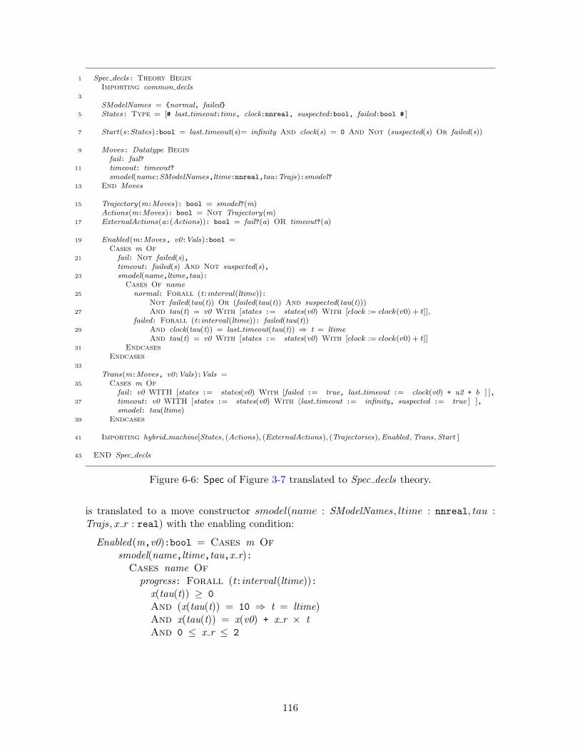
1 Spec decls: Theory BeginImporting common decls
3
SModelNames = normal, failed5 States: Type = [# last timeout:time, clock:nnreal, suspected:bool, failed:bool # ]
7 Start(s:States):bool = last timeout(s)= infinity And clock(s) = 0 And Not (suspected(s) Or failed(s))
9 Moves: Datatype Beginfail: fail?
11 timeout: timeout?smodel(name:SModelNames,ltime:nnreal,tau:Trajs):smodel?
13 End Moves
15 Trajectory(m:Moves): bool = smodel?(m)Actions(m:Moves): bool = Not Trajectory(m)
17 ExternalActions(a:(Actions)): bool = fail?(a) OR timeout?(a)
19 Enabled(m:Moves, v0:Vals):bool =Cases m Of
21 fail: Not failed(s),timeout: failed(s) And Not suspected(s),
23 smodel(name,ltime,tau):Cases Of name
25 normal: Forall (t:interval(ltime)):Not failed(tau(t)) Or (failed(tau(t)) And suspected(tau(t)))
27 And tau(t) = v0 With [states := states(v0) With [clock := clock(v0) + t]],failed: Forall (t:interval(ltime)): failed(tau(t))
29 And clock(tau(t)) = last timeout(tau(t)) ⇒ t = ltimeAnd tau(t) = v0 With [states := states(v0) With [clock := clock(v0) + t]]
31 EndcasesEndcases
33
Trans(m:Moves, v0:Vals):Vals =35 Cases m Of
fail: v0 WITH [states := states(v0) With [failed := true, last timeout := clock(v0) + u2 + b ] ],37 timeout: v0 WITH [states := states(v0) With 〈last timeout := infinity, suspected := true ] ],
smodel: tau(ltime)39 Endcases
41 Importing hybrid machine[States, (Actions), (ExternalActions), (Trajectories),Enabled ,Trans,Start ]
43 END Spec decls
Figure 6-6: Spec of Figure 3-7 translated to Spec decls theory.
is translated to a move constructor smodel(name : SModelNames, ltime : nnreal, tau :Trajs, x r : real) with the enabling condition:
Enabled(m,v0):bool = Cases m Ofsmodel(name,ltime,tau,x r):
Cases name Ofprogress: Forall (t:interval(ltime)):
x(tau(t)) ≥ 0And (x(tau(t)) = 10 ⇒ t = ltime)And x(tau(t)) = x(v0) + x r × tAnd 0 ≤ x r ≤ 2
116

1 automaton Timeout(M :type,u1, u2, b : Real)where u1 ≥ 0 ∧u2 ≥ 0 ∧ b ≥ 0 ∧u2 > (u1 + b)
3 signatureinternal send(m : M), receive(m : M)
5 output fail, timeout
7 variablesinternal next send : AugmentedReal := 0;
9 next recv : AugmentedReal := u2;suspected : Bool := false;
11 failed : Bool := false;now, clockp, clockd : Real := 0;
13 queue : Seq[Packet] := ;
15 transitionsinternal send(m)
17 pre 6= failed ∧next send = clockp;eff next send := clockp + u1;
19 queue := queue ` [m,now + b];
21 internal receive(m)pre m = head(queue);
23 eff next recv := clockd + u2;queue := tail(queue);
25
output fail27 pre ¬failed;
eff failed := true;29 clockp := ∞;
31 output timeoutpre ¬suspected ∧ clockd = next recv;
33 eff suspected := true;next recv := ∞;
36trajectoriestrajdef normal
38stop when (next send = clockp) ∨(next recv = clockd) ∨
40(now = head(queue).deadline);evolve d(now) = 1;
42d(clockp) = 1; d(clockd) = 1;
44invariant of Timeout:clockp = clockd = now >= 0;
46
invariant of Timeout: clockd ≤ next recv ∧48clockp ≤ next send ∧
now <= head(queue).deadline;50
invariant of Timeout: (now + u2) >= 0 ∧52¬suspected⇒ next recv 6= ∞ ∧
next recv ≤ (now + u2);54
invariant of Timeout: (now + u1) >= 0 ∧56¬failed⇒ next send 6= ∞ ∧
next send ≤ (now + u1);58
invariant of Timeout: ∀n : Nat60(n ≤ (length(queue)− 1) ⇒
deadline(queue[n]) ≤ (now + b));62
invariant of Timeout: ¬failed⇒ if queue 6= 64then head(queue).deadline < next recv
else (next send+ b) < next recv;66
invariant of Timeout: suspected ≥ failed;
Figure 6-7: Timeout automaton in HIOA .
6.2.8 Invariants
The hybrid machine theory is a generic SHIOA library theory which provides several essen-tial definitions and lemmas for SHIOAs. This theory is quite similar to the existing TAMEtheory [AHS98] for timed I/O automaton. In Section 6.3 we will describe in detail howthese definitions and lemmas are used by our specialized strategies that automate proofs.In this subsection and the next one, we describe how these definitions are used for statinginvariant properties and implementation relations.
Each translated theory imports hybrid machine with the parameters States, (Actions),(ExternalActions), (Trajectory), Enabled ,Trans, and Start , based on which the followingfunctions are defined.
Reachable hidden(v,n:nat): Recursive bool = If n = 0 Then Start(local(v))Else (Exists m, v1:Vals): Reachable hidden(v1,n -1) And
Enabled(m,v1) And v = Trans(m,v1)) EndifMeasure Lambda v,n: nReachable(s):bool = Exists (n:nat,v): Reachable hidden(v,n) And states(v) = s
In the above fragment, s,m, and v are global variables of type States, Moves, and Vals,respectively, and Inv is any predicate on States. The predicate Reachable hidden(n, v) isdefined recursively and it returns true if the valuation v of the variables can be reachedthrough a sequence of n Moves. The predicate Reachable(s) returns true if there exists a
117
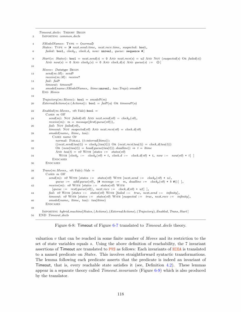
Timeout decls: Theory Begin2 Importing common decls
4 SModelNames: Type = normalStates: Type = [# next send:time, next recv:time, suspected: bool,
6 failed: bool, clockp, clock d, now: nnreal, queue: sequence # ]
8 Start(s: States): bool = next send(s) = 0 And next recv(s) = u2 And Not (suspected(s) Or failed(s))And now(s) = 0 And clockp(s) = 0 And clock d(s) And queue(s) := ]
10
Moves: Datatype Begin12 send(m:M): send?
receive(m:M): receive?14 fail: fail?
timeout: timeout?16 smodel(name:SModelNames, ltime:nnreal, tau:Trajs):smodel?
End Moves18
Trajectory(m:Moves): bool = smodel?(m)20 ExternalActions(a:(Actions)): bool = fail?(a) Or timeout?(a)
22 Enabled(m:Moves, v0:Vals):bool =Cases m OF
24 send(m): Not failed(v0) And next send(v0) = clockp(v0),receive(m): m = message(first(queue(v0))),
26 fail: Not failed(v0),timeout: Not suspected(v0) And next recv(v0) = clock d(v0)
28 smodel(name, ltime, tau):Cases name Of
30 normal: Forall (t:interval(ltime)):((next send(tau(t)) = clockp(tau(t))) Or (next recv(tau(t)) = clock d(tau(t)))
32 Or (now(tau(t)) = head(queue(tau(t))).deadline)) ⇒ t = ltimeAnd tau(t) = v0 With [states := states(v0)
34 With [clockp := clockp(v0) + t, clock d := clock d(v0) + t, now := now(v0) + t ] ]Endcases
36 Endcases
38 Trans(m:Moves, v0:Vals):Vals =Cases m OF
40 send(m): v0 With [states := states(v0) With [next send := clockp(v0) + u1,queue := add(queue(v0), (# message := m, deadline := clockp(v0) + b #)) ] ],
42 receive(m): v0 With [states := states(v0) With[queue := rest(queue(v0)), next recv := clock d(v0) + u2 ] ],
44 fail: v0 With [states := states(v0) With [failed := true, next send := infinity ],timeout: v0 With [states := states(v0) With [suspected := true, next recv := infinity ],
46 smodel(name, ltime, tau): tau(ltime)Endcases
48
Importing hybrid machine[States, (Actions), (ExternalActions), (Trajectory),Enabled ,Trans,Start ]50 END Timeout decls
Figure 6-8: Timeout of Figure 6-7 translated to Timeout decls theory.
valuation v that can be reached in some finite number of Moves and its restriction to theset of state variables equals s. Using the above definition of reachability, the 7 invariantassertions of Timeout are translated to PVS as follows: Each invariants of HIOA is translatedto a named predicate on States. This involves straightforward syntactic transformations.The lemma following each predicate asserts that the predicate is indeed an invariant ofTimeout, that is, every reachable state satisfies it (see, Definition 4.2). These lemmasappear in a separate theory called Timeout invariants (Figure 6-9) which is also producedby the translator.
118
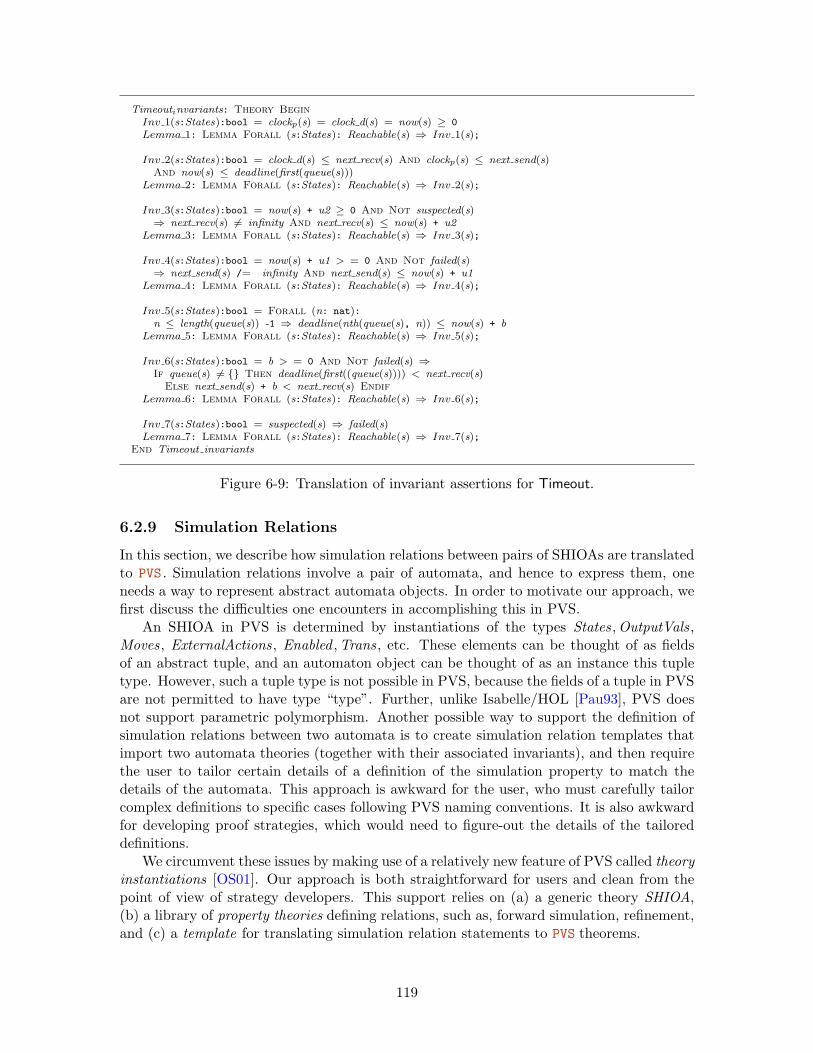
Timeoutinvariants: Theory BeginInv 1(s:States):bool = clockp(s) = clock d(s) = now(s) ≥ 0
Lemma 1: Lemma Forall (s:States): Reachable(s) ⇒ Inv 1(s);
Inv 2(s:States):bool = clock d(s) ≤ next recv(s) And clockp(s) ≤ next send(s)And now(s) ≤ deadline(first(queue(s)))
Lemma 2: Lemma Forall (s:States): Reachable(s) ⇒ Inv 2(s);
Inv 3(s:States):bool = now(s) + u2 ≥ 0 And Not suspected(s)⇒ next recv(s) 6= infinity And next recv(s) ≤ now(s) + u2
Lemma 3: Lemma Forall (s:States): Reachable(s) ⇒ Inv 3(s);
Inv 4(s:States):bool = now(s) + u1 > = 0 And Not failed(s)⇒ next send(s) /= infinity And next send(s) ≤ now(s) + u1
Lemma 4: Lemma Forall (s:States): Reachable(s) ⇒ Inv 4(s);
Inv 5(s:States):bool = Forall (n: nat):n ≤ length(queue(s)) -1 ⇒ deadline(nth(queue(s), n)) ≤ now(s) + b
Lemma 5: Lemma Forall (s:States): Reachable(s) ⇒ Inv 5(s);
Inv 6(s:States):bool = b > = 0 And Not failed(s) ⇒If queue(s) 6= Then deadline(first((queue(s)))) < next recv(s)
Else next send(s) + b < next recv(s) EndifLemma 6: Lemma Forall (s:States): Reachable(s) ⇒ Inv 6(s);
Inv 7(s:States):bool = suspected(s) ⇒ failed(s)Lemma 7: Lemma Forall (s:States): Reachable(s) ⇒ Inv 7(s);
End Timeout invariants
Figure 6-9: Translation of invariant assertions for Timeout.
6.2.9 Simulation Relations
In this section, we describe how simulation relations between pairs of SHIOAs are translatedto PVS . Simulation relations involve a pair of automata, and hence to express them, oneneeds a way to represent abstract automata objects. In order to motivate our approach, wefirst discuss the difficulties one encounters in accomplishing this in PVS.
An SHIOA in PVS is determined by instantiations of the types States,OutputVals,Moves, ExternalActions, Enabled ,Trans, etc. These elements can be thought of as fieldsof an abstract tuple, and an automaton object can be thought of as an instance this tupletype. However, such a tuple type is not possible in PVS, because the fields of a tuple in PVSare not permitted to have type “type”. Further, unlike Isabelle/HOL [Pau93], PVS doesnot support parametric polymorphism. Another possible way to support the definition ofsimulation relations between two automata is to create simulation relation templates thatimport two automata theories (together with their associated invariants), and then requirethe user to tailor certain details of a definition of the simulation property to match thedetails of the automata. This approach is awkward for the user, who must carefully tailorcomplex definitions to specific cases following PVS naming conventions. It is also awkwardfor developing proof strategies, which would need to figure-out the details of the tailoreddefinitions.
We circumvent these issues by making use of a relatively new feature of PVS called theoryinstantiations [OS01]. Our approach is both straightforward for users and clean from thepoint of view of strategy developers. This support relies on (a) a generic theory SHIOA,(b) a library of property theories defining relations, such as, forward simulation, refinement,and (c) a template for translating simulation relation statements to PVS theorems.
119

SHIOA:Theory BeginStates: Types+ExternalVals: TypesLocalVals: TypesMoves: Types+Actions(m:Moves):boolTrajectories(m:Moves):boolInternalActions(a:(Actions)):boolExternalActions(a:(Actions)):boolStart(s:States):boolEnabled(m:Moves, v:Vals):boolTrans(m:Moves, v:Vals):Vals
Trajs(t:nnreal): TypesExtTrajs(t:nnreal): Typesstates(v:(Vals)):Statesexttraj (m:(Trajectories)):ExtTrajs
Reachable(s:States):boolInvisibleSeqReach(s,s1:States):boolVisibleContReach(s,s1:States,t:nnreal,
trace:ExtTrajs):boolEnd SHIOAutomaton
Figure 6-10: SHIOA PVS theory.
The SHIOA Theory
Figure 6-10 shows the SHIOA theory, which declares the elements that specify an SHIOA.Other than the pattern of type restrictions, the SHIOA theory makes no other restrictionson the elements. Note that the translation scheme we have described in Sections 3.2-3.6,precisely defines these elements for particular SHIOAs. That is, the names and types ofelements in SHIOA theory match exactly the names and types of the definitions that appearin PVS translation of HIOA specifications. Henceforth, we shall say that a PVS theory ob-tained by translating a HIOA automaton specification, such as Timeout decls, is an instanceof the SHIOA theory. Instantiation of SHIOA provides concrete definitions of the SHIOA’selements. The concrete definitions for the first set of these elements are written by theuser when writing a HIOA specification and then this information is translated to the corre-sponding PVS theory. The remaining elements are the same for all SHIOAs automata andare defined in the hybrid machine library library. The user does not have to redefine themfor specific automata, because an appropriate instance of hybrid machine is imported in thetranslated specification. We have defined all but the last two elements in this theory. Thepredicate InvisibleSeqReach(s1, s2) is true if and only if there exists an execution fragmentα = τ0a1τ1a2 . . . τn such that α.fstate = s1, α.lstate = s2, all the τi’s are point trajectoriesand all the ai’s are internal actions. Finally, VisibleContReach(s1, s2, t, trace) is true ifand only if there exists an execution fragment α = τ0a1τ1a2 . . . τn such that α.fstate = s1,α.lstate = s2, α.ltime = t, all the ai’s are internal actions, and the restriction of α toexternal variables and actions equals trace. Both these predicates is defined inductively interms of the number of internal actions (and trajectories) constituting α.
Property Theories
The Forward simulation theory shown in Figure 6-11 is a typical property theory ; it defineswhat it means for a relation R to be a forward simulation relation between a pair of genericSHIOAs. In the same spirit we are developing property theories for homorphism, weakrefinement, switching simulation, and backward simulation—all of which involve pairs ofSHIOAs. The first two parameters Forward simulation are of type Theory SHIOA. Thismeans that
Importing Forward simulation[Theory1 decls,Theory2 decls, . . . , . . .]
automatically instantiates the elements of SHIOA theory with two sets of definitions, cor-responding to those appearing in Theory1 decls and Theory2 decls. For example, the type
120

A.States, is matched with the type States of Theory1 decls. The third parameter R is arelation on the states of A and B, which is the putative forward simulation relation. Inthe mathematical definition of a forward simulation (Definition 4.3), every move of A ismatched by a sequence of moves of B with the same trace such that the final states arerelated. Since the type ExternalActions (and ExternalVals) of A is defined completely in-dependently of the type ExternalActions (ExternalVals, resp.) of B, we cannot equate anexternal action (trajectory of an external variables) of A with that of B. For this reason,we have to map each external action (variable) of A to an external action (variable) ofB. The last two parameters of Forward simulation, namely, ExtActMap and ExtValMap,provide these maps. While often these functions map an action (variable) of A to an action(variable) of B with the same name, they do provide a mechanism for relating automatawith completely different action (and variable) names.
Recall the definition of a forward simulation relation from Chapter 4. The first con-dition of Definition 4.3, that is, the base case is captured by the FwdSimBase predicate(line 10). The second and the third conditions of are combined into the FwdSimInd predi-cate (lines 12–24). FwdSimInd returns true if for all states s A, s1 A of A, state s B of Band for all moves m of A the following three conditions hold: (1) s A and s B are related byR and are reachable states of A and B, respectively (line 12). (2) There exist appropriatevaluations of the variables of A such that the move m takes the state s A to s1 A (line 14).(3) And Finally, based on the type of the move m one of the following conditions must hold(lines 15–24):
Case 1: m is an external action of A (lines 15–18). There exist intermediate valuationsv1 B, v2 B, and a state s1 B of B such that s1 A and s1 B are related by R, and(i) sB can go to states(v1 B) through a sequence of internal actions (no time passage),(ii) states(v2 B) can go to s1 B through a sequence of internal actions, (iii) v1 B goesto v2 B by performing the external action ExtActMap(m).
Case 2: m is an internal action of A (line 20). There exists a state s1 B of B such thats1 A and s1 B are related by R and s B can go to s1 B through a sequence of internalactions.
Case 3: m is a trajectory of A (line 23). There exists a state s1 B of B and a nonnegativereal number t, such that s1 A and s1 B are related by R and s B can go to s1 Bthrough a sequence of alternating trajectories and internal actions such that the traceof the whole sequence is ExtVarMap(tau(m)) and has length t.
The FwdSim predicate combines FwdSimBase FwdSimInd for the given pair of SHIOAs,the relation R, and the external action and external variable maps.
Translation of Simulation Relations to PVS
With the SHIOA and the Forward simulation theories in place, we are in a position totranslate HIOA statements that define simulation relations between a pair of automata. Thetranslation takes the form of a separate theory such as the one shown in Figure 6-12. ThePVS theories generated by translating each of the HIOA automata specifications are imported,and then these theories are interpreted as instances of the SHIOA theory using the syntax
MA: Theory = SHIOA :→ Timeout decls
121

1 Forward simulation[A,B: Theory SHIOA, R: [A.States, B.States → bool ]ExtActMap: [(A.ExternalActions) → (B.ExternalActions) ],
3 ExtVarMap: [(A.ExternalVals) → (B.ExtrnalVals) ] ]: Theory Begin
5 m : Var A.Movess A, s1 A: Var A.States
7 s B, s1 B: Var B.Statesv1 B,v2 B: Var B.Vals
9
FwdSimBase: bool = Forall s A: A.Start(s A) ⇒ Exists(s B): B.Start(s B) And R(s A,s B)11
FwdSimInd: bool = Forall s A,s1 A,s B,m: A.Reachable(s A) And B.Reachable(s B) And R(s A,s B)13 And Exists v A,v1 A: states(v A) = s A And states(v1 A) = s1 A
And A.Enabled(m,s A) And v1 A = A.Trans(m,v A) ⇒15 (A.ExternalActions(m) ⇒ Exists (v1 B,v2 B,s1 B):
B.InvisibleSeqReach(s B,states(v1 B)) And B.InvisibleSeqReach(states(v2 B),s1 B) And17 B.Enabled(ExtActMap(m),v1 B) And
B.Trans(ExtActMap(m),v1 B) = v2 B And R(s1 A, s1 B))19 And
(A.InternalActions(m) And A.Actions(m)) ⇒ Exists (s1 B):21 B.InvisibleSeqReach(s B,s1 B) And R(s1 A, s1 B)
And23 (A.Trajectories(m) ⇒ Exists (t:nnreal, s1 B):
B.VisibleContReach(s B,s1 B,t,ExtVarMap(t,exttraj (m))) And R(s1 A, s1 B))25
FwdSim:bool = FwdSimBase And FwdSimInd27 End Forward simulation
Figure 6-11: Forward simulation theory.
This matches the elements of SHIOA with their corresponding definitions in Timeout declsand makes them available as components of MA. The function ExtActMap maps the twoexternal actions of Timeout decls, namely, fail and timeout, to the identically namedexternal actions of Spec decls. Since neither automata have external variables, the functionExtVarMap is declared but is left uninterpreted. It does not impose any constrains apartfrom the fact that a trajectory move m of MA should be matched with a sequence oftrajectories and actions of MB with a total length ltime(m). The relation R on the statesofMA andMB is the putative forward simulation relation from Timeout to Spec. ImportingForward simulation defines the FwdSim predicate of Figure 6-11 for the automaton theoriesTimeout decls and Spec decls. Finally, the FwdSimThm theorem simply asserts that theFwdSim predicate holds, that is, R satisfies all the conditions to be a forward simulationrelation.
6.3 Strategies
In the previous section we have described how HIOA specifications of automata and theirproperties such as invariant assertions and simulation relations can be translated to PVS .Once translated, the proofs of theorems and lemmas, such as those in Figures 6-9 and 6-12,can be constructed interactively by invoking the PVS theorem prover. The PVS theo-rem prover provides a set of general proof commands for manipulating logical formulas.Basic proof commands include commands for simplification of expressions, expansion ofdefinitions, and instantiation of existentially quantified variables. The PVS prover alsoprovides more powerful commands for automated theorem proving such as general semi-decision procedures for first and higher order logics and an infinite bounded model-checker.Notwithstanding the power of the PVS prover, we have found that construction of invariant
122
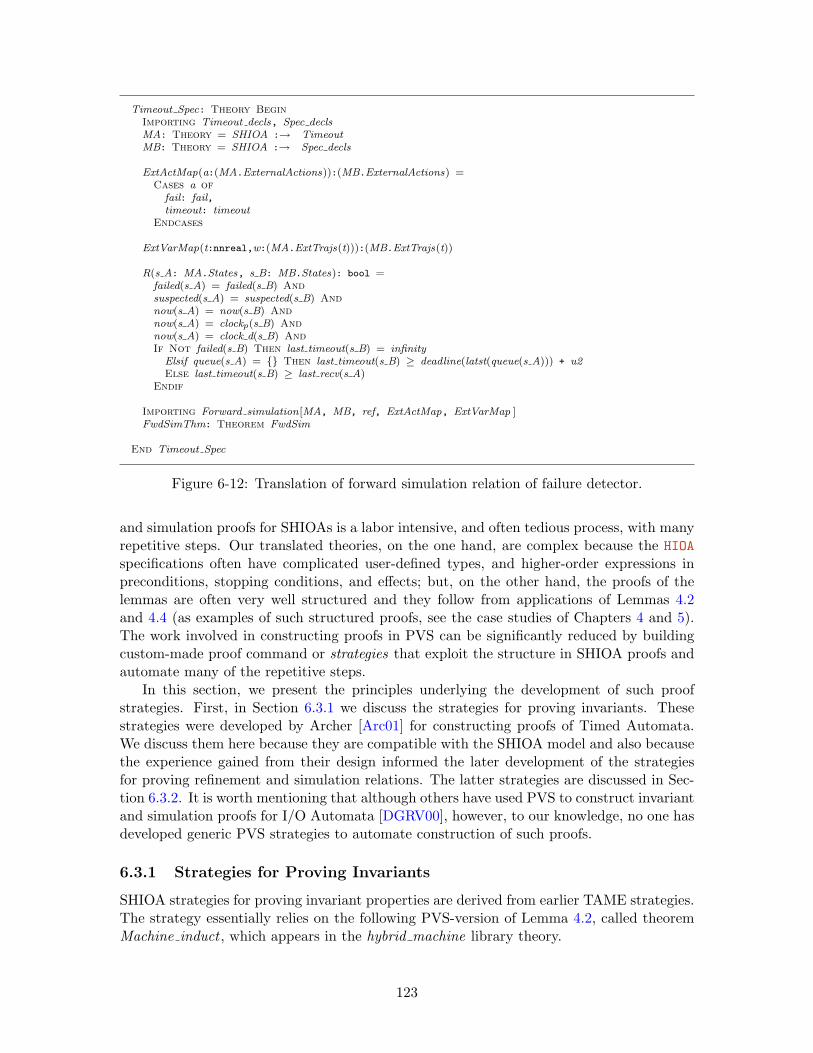
Timeout Spec: Theory BeginImporting Timeout decls, Spec declsMA: Theory = SHIOA :→ TimeoutMB: Theory = SHIOA :→ Spec decls
ExtActMap(a:(MA.ExternalActions)):(MB.ExternalActions) =Cases a of
fail: fail,timeout: timeout
Endcases
ExtVarMap(t:nnreal,w:(MA.ExtTrajs(t))):(MB.ExtTrajs(t))
R(s A: MA.States, s B: MB.States): bool =failed(s A) = failed(s B) Andsuspected(s A) = suspected(s B) Andnow(s A) = now(s B) Andnow(s A) = clockp(s B) Andnow(s A) = clock d(s B) AndIf Not failed(s B) Then last timeout(s B) = infinity
Elsif queue(s A) = Then last timeout(s B) ≥ deadline(latst(queue(s A))) + u2Else last timeout(s B) ≥ last recv(s A)
Endif
Importing Forward simulation[MA, MB, ref, ExtActMap, ExtVarMap ]FwdSimThm: Theorem FwdSim
End Timeout Spec
Figure 6-12: Translation of forward simulation relation of failure detector.
and simulation proofs for SHIOAs is a labor intensive, and often tedious process, with manyrepetitive steps. Our translated theories, on the one hand, are complex because the HIOAspecifications often have complicated user-defined types, and higher-order expressions inpreconditions, stopping conditions, and effects; but, on the other hand, the proofs of thelemmas are often very well structured and they follow from applications of Lemmas 4.2and 4.4 (as examples of such structured proofs, see the case studies of Chapters 4 and 5).The work involved in constructing proofs in PVS can be significantly reduced by buildingcustom-made proof command or strategies that exploit the structure in SHIOA proofs andautomate many of the repetitive steps.
In this section, we present the principles underlying the development of such proofstrategies. First, in Section 6.3.1 we discuss the strategies for proving invariants. Thesestrategies were developed by Archer [Arc01] for constructing proofs of Timed Automata.We discuss them here because they are compatible with the SHIOA model and also becausethe experience gained from their design informed the later development of the strategiesfor proving refinement and simulation relations. The latter strategies are discussed in Sec-tion 6.3.2. It is worth mentioning that although others have used PVS to construct invariantand simulation proofs for I/O Automata [DGRV00], however, to our knowledge, no one hasdeveloped generic PVS strategies to automate construction of such proofs.
6.3.1 Strategies for Proving Invariants
SHIOA strategies for proving invariant properties are derived from earlier TAME strategies.The strategy essentially relies on the following PVS-version of Lemma 4.2, called theoremMachine induct , which appears in the hybrid machine library theory.
123
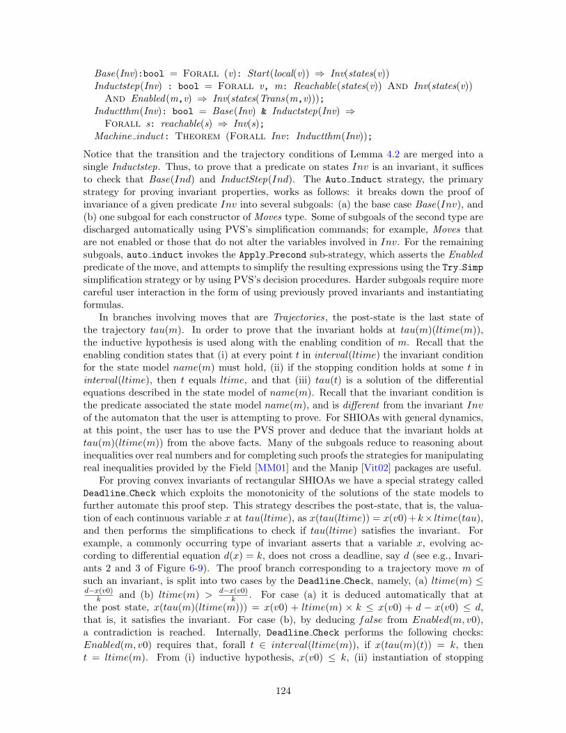
Base(Inv):bool = Forall (v): Start(local(v)) ⇒ Inv(states(v))Inductstep(Inv) : bool = Forall v, m: Reachable(states(v)) And Inv(states(v))
And Enabled(m,v) ⇒ Inv(states(Trans(m,v)));Inductthm(Inv): bool = Base(Inv) & Inductstep(Inv) ⇒
Forall s: reachable(s) ⇒ Inv(s);Machine induct: Theorem (Forall Inv: Inductthm(Inv));
Notice that the transition and the trajectory conditions of Lemma 4.2 are merged into asingle Inductstep. Thus, to prove that a predicate on states Inv is an invariant, it sufficesto check that Base(Ind) and InductStep(Ind). The Auto Induct strategy, the primarystrategy for proving invariant properties, works as follows: it breaks down the proof ofinvariance of a given predicate Inv into several subgoals: (a) the base case Base(Inv), and(b) one subgoal for each constructor of Moves type. Some of subgoals of the second type aredischarged automatically using PVS’s simplification commands; for example, Moves thatare not enabled or those that do not alter the variables involved in Inv. For the remainingsubgoals, auto induct invokes the Apply Precond sub-strategy, which asserts the Enabledpredicate of the move, and attempts to simplify the resulting expressions using the Try Simpsimplification strategy or by using PVS’s decision procedures. Harder subgoals require morecareful user interaction in the form of using previously proved invariants and instantiatingformulas.
In branches involving moves that are Trajectories, the post-state is the last state ofthe trajectory tau(m). In order to prove that the invariant holds at tau(m)(ltime(m)),the inductive hypothesis is used along with the enabling condition of m. Recall that theenabling condition states that (i) at every point t in interval(ltime) the invariant conditionfor the state model name(m) must hold, (ii) if the stopping condition holds at some t ininterval(ltime), then t equals ltime, and that (iii) tau(t) is a solution of the differentialequations described in the state model of name(m). Recall that the invariant condition isthe predicate associated the state model name(m), and is different from the invariant Invof the automaton that the user is attempting to prove. For SHIOAs with general dynamics,at this point, the user has to use the PVS prover and deduce that the invariant holds attau(m)(ltime(m)) from the above facts. Many of the subgoals reduce to reasoning aboutinequalities over real numbers and for completing such proofs the strategies for manipulatingreal inequalities provided by the Field [MM01] and the Manip [Vit02] packages are useful.
For proving convex invariants of rectangular SHIOAs we have a special strategy calledDeadline Check which exploits the monotonicity of the solutions of the state models tofurther automate this proof step. This strategy describes the post-state, that is, the valua-tion of each continuous variable x at tau(ltime), as x(tau(ltime)) = x(v0)+k× ltime(tau),and then performs the simplifications to check if tau(ltime) satisfies the invariant. Forexample, a commonly occurring type of invariant asserts that a variable x, evolving ac-cording to differential equation d(x) = k, does not cross a deadline, say d (see e.g., Invari-ants 2 and 3 of Figure 6-9). The proof branch corresponding to a trajectory move m ofsuch an invariant, is split into two cases by the Deadline Check, namely, (a) ltime(m) ≤d−x(v0)
k and (b) ltime(m) > d−x(v0)k . For case (a) it is deduced automatically that at
the post state, x(tau(m)(ltime(m))) = x(v0) + ltime(m) × k ≤ x(v0) + d − x(v0) ≤ d,that is, it satisfies the invariant. For case (b), by deducing f alse from Enabled(m, v0),a contradiction is reached. Internally, Deadline Check performs the following checks:Enabled(m, v0) requires that, forall t ∈ interval(ltime(m)), if x(tau(m)(t)) = k, thent = ltime(m). From (i) inductive hypothesis, x(v0) ≤ k, (ii) instantiation of stopping
124

x(tau(m)(ltime(m))) > x(v0) + k × d−x(v0)k = k, and (iii) monotonicity of x(tau(m)),
that is, ∀t ∈ interval(ltime(m)), x(tau(t)) = x(v0) + k × t, it is deduced that there existst ∈ interval(ltime(m)), such that x(tau(t)) = d but t 6= ltime(m)—a contradiction withEnabled(m, v0). Thus, in case (b) m is not a valid move of the automaton in question andtherefore this branch of the induction proof is complete.
6.3.2 Strategies for Proving Forward Simulation
In this section, we discuss strategies we have developed for proving forward simulationrelations for SHIOAs. These strategies were originally developed for Timed I/O Automataalong with several other strategies for proving weak-refinement [MA03, MA05].
The main strategy for proving forward simulations, as defined by the Forward simulationtheory, is called Prove Fwd Sim. The generic nature of the definition of the FwdSim prop-erty allows us to define Prove Fwd sim in such a way that it can be applied to an arbitrarysimulation proof between any given pair of SHIOAs. This strategy is designed to per-form much of the work, for an arbitrary simulation theorem such as the one stated atthe end of the Timeout Spec theory. The structure of Prove Fwd Sim in terms of sub-strategies is shown in Figure 6-16. The branches terminating in blue circles signify thatthe if the preceding sub-strategy fails to complete the proof, the resulting subgoals arehanded over to the user for constructing their proofs interactively. First, Prove Fwd Simsplits the predicate FwdSim into FwdSimBase and FwdSimInd and applies Setup Sim Baseand Setup Sim Induct Cases sub-strategies to the branches, respectively. Setup Sim Baseperforms the standard steps needed in the base case, including skolemization, expansion ofthe definitions Start and R, and simplifications. The base case sequent, which is han-dled by Setup Sim Base, is shown in Figure 6-13, in which Timout decls.Start andSPEC decls.start are the start predicates of Timeout and Spec, respectively. Prove Fwd Sim
;;;Base case
-1 Timeout_decls.Start(s_A)
|-------
1 Exists (s_B:Spec_decls.States): Spec_decls.Start(s_B) And R(s_A,s_B)
Figure 6-13: Base case sequent of simulation proof.
then probes the proof state to check if the base case can be discharged trivially, and then, itmoves over to the next branch of the proof, namely, the application of Setup Sim Induct Casesto FwdSimInd . If a proof subgoal is not completely resolved by the application of a strat-egy, then the final set of sequents produced by the strategy are presented to the user forinteractive proving.
The sub-strategy Setup Sim Induct Cases performs skolemization and expands the def-initions of InternalActions, ExternalActions, and Trajectories and splits up the inductionstep into a set of subgoals—one for each constructor of the Moves datatype. Based onwhether the constructor classifies as ExternalActions, InternalActions, or Trajectories, theSim Induct ExtAction, the Sim Induct IntAction, or the Sim Induct Traj sub-strategiesare applied. In what follows, we will discuss each of these sub-strategies, but first we dis-cuss a strategy called State Trans which is a building-block for all these strategies. TheState Trans strategy is used for constructing states by applying a sequence of moves toa given state. Thus, this strategy is useful for proving the InvisibleSeqReach predicatewhich appear in the definition of FwdSimInd . This strategy takes a sequence of action, say
125

σ = a0, a1, . . . , an, a starting valuation v1, and a target state s2 as parameters and producesthe following set of subgoals:
s2 = state(Trans(an,Trans(an−1,Trans(an−2, . . . ,Ttrans(a1, v1) . . .)))),
For each i ∈ 1, . . . , n, InternalActiona(ai), and
For each i ∈ 1, . . . , n, Enabled(ai,Trans(ai−1,Trans(ai−2, . . . , v1) . . .).
For an appropriate sequence of internal actions, the strategy then discharges the firstand the second set of subgoals by expanding the definitions of InternalActions,Enabled ,and Trans. The remaining subgoals are then presented to the user with properly la-beled sequents. Instances of this strategy are used by the Sim Induct ExtAction andthe Sim Induct IntAction sub-strategies as discussed below.
The Sim Induct IntAction strategy is designed for proving the second case (line 21) inthe definition of FwdSimInd of Figure 6-11. This strategy prompts the user for a sequence
;;;Induction step: internal action Case "send"
[-1, (reachable A.prestate)] A.Reachable(s_A)
[-2, (reachable B.prestate)] B.Reachable(s_B)
[-3, (related A.prestate B.prestate)] R(s_A,s_B)
[-4, (send A.move)] send?(m)
[-5, (enabled A.action)] A.Enabled(m,s_A)
[-6] s1_A = states(v1_A)
[-7] v1_A = A.Trans(m,v_A)
|-------
1 Exists (s1_B:Spec_decls.States): B.InvisibleSeqReach(s_B,s1_B) And R(s1_A, s1_B))
Figure 6-14: Inductive step sequent for internal actions.
of internal actions σ of automaton B. This is the sequence of actions that will be used tomatch the move m of automaton A and this sequence will take state s B to s1 B. Formally,s1 B is instantiated as Trans(σ, s B) and the branch generates the subgoals: (i) s B reachess1 B through a sequence of internal actions, (ii) s1 B and s1 A are related by R.
For example, consider the sequent it Figure 6-14, which is an intermediate subgoal inthe inductive branch corresponding to moves constructed using the send constructor ofTimeout . This corresponds to the proof branch in a hand-proof for an the internal sendaction of Timeout. The first line of the sequent is a comment added by the strategy whichindicates the current branch of the proof. All the variables appearing in the antecedentare constants resulting from skolemizing universally quantified expressions. Suppose inproving this branch, the user invokes the Sim Induct IntAction strategy with parameter“ ”, indicating that the send action of Timeout is emulated by Spec by an empty sequenceof actions. Then, s1 B is instantiated as State Trans(“ ”,s B) which of course is identicalto s B. In the resulting sequent, s1 B is replaced by s B; B.InvisibleSeqReach(s B, s B)holds trivially and is proved automatically by the State Trans strategy. Therefore, sequentreduces to proving R(s1 A, s B) which is deduced from the hypothesis R(s A, s B) andfrom the definition of Trans. This last bit of simplification is performed by the Do Transsub-strategy which computes the post-state from a pre-state by applying a transition andrepeatedly simplifies. In this case, s1 A is computed by applying a send transition to s A.In general, when State Trans strategy is called with a sequence of actions of length n, thenfor each action an enablement-subgoeal is produced which is delegated to an Enablement
126

sub-strategy. The Enablement sub-strategy expands the definition of the Enabled predicateand simplifies to prove that the move in question is enabled at a given state.
The Sim Induct ExtAction sub-strategy is used to prove branches corresponding tomoves that are ExternalActions. This strategy prompts the user for two sequences of inter-nal actions, say σa and σ2. These sequences are used to construct a sequence σ1ExtActMap(m)σ2,which matches the move m of automaton A.
Consider a typical sequent of this type as shown in Figure 6-15 which is an induc-tive branch corresponding to moves constructed using the fail constructor. As in thecase of internal actions, the first line of the sequent is a comment added by the strat-egy and all the variables appearing skolem constants. The requirement for this branchis to show the existence of a valuations v1 B, v2 B, and state s1 B, such that (i) s Breaches v1 B through a sequence of internal actions, (ii) v2 B reaches s1 B through asequence of internal actions, (iii) v1 B reaches v2 B through an action ExtActMap(m),and (iv) s1 B and s1 A are related by R. Sim Induct ExtAction instantiates v1 B, v2 B,and s1 B by applying State Trans strategy as follows: v1 B = State Trans(σ1, s B),v2 B = Trans(ExtActMap(m), v1 B), and s1 B = states(State Trans(σ2, v2 B)). Once
;;;Induction step: external action Case "fail"
[-1, (reachable A.prestate)] A.Reachable(s_A)
[-2, (reachable B.prestate)] B.Reachable(s_B)
[-3, (related A.prestate B.prestate)] R(s_A,s_B)
[-4, (fail A.move)] fail?(m)
[-5, (enabled A.action)] A.Enabled(m,s_A)
[-6] s1_A = states(v1_A)
[-7] v1_A = A.Trans(m,v_A)
|-------
1 Exists (v1_B,v2_B:Spec_decls.Vals,s1_B:Spec_decls.States):
B.InvisibleSeqReach(s_B,states(v1_B)) And B.InvisibleSeqReach(states(v2_B),s1_B) And
B.Enabled(ExtActMap(m),v1_B) And B.Trans(ExtActMap(m),v1_B) = v2_B And R(s1_A, s1_B))
Figure 6-15: Inductive step sequent for external actions.
instantiated, the resulting sequent is split into the above four branches. Branches (i), (ii)and (iv) are handled the same way as in the case of internal actions. Branch (iii) requiresan additional application of the Enablement and the Do Trans strategies. All these appli-cations are automated by the Sim Induct ExtAction strategy and any subgoals that arenot completely proved are handed back to the user.
The Sim Induct Traj strategy is designed for proving the last case (line 23) in the def-inition of FwdSimInd of Figure 6-11. At the onset, the trajectory spits up the proof intoseveral cases, one for each element in the type SModelNames, and applies the Induct Smodelsub-strategy to each case. For example, the intermediate sequent in Figure 6-17, appears inthe inductive branch corresponding to trajectory moves of Timeout at the point in whichInduct Smodel is invoked. In Timeout there is a single state model, that is, SModelNamesis a singleton type and therefore this is the only branch corresponding to trajectory moves.Note that the fifth expression in the antecedent asserts the name of the state model branch.The Induct Smodel allows the user to construct an execution fragment of B that emu-lates the trajectory tau(m) of A. The strategy prompts the user for a four parameters:(a) a natural number n, (b) a sequence s0, . . . , sn of elements of type SModelNames, (c) asequence a1, . . . , an−1 of internal actions, and (d) a sequence t0, . . . , tn of positive reals sum-ming to ltime(m). From these parameters it implicitly constructs an execution fragmentτ0a1τ1a2 . . . τn of n + 1 trajectories and n transitions. The first trajectory τ0 is defined as
127
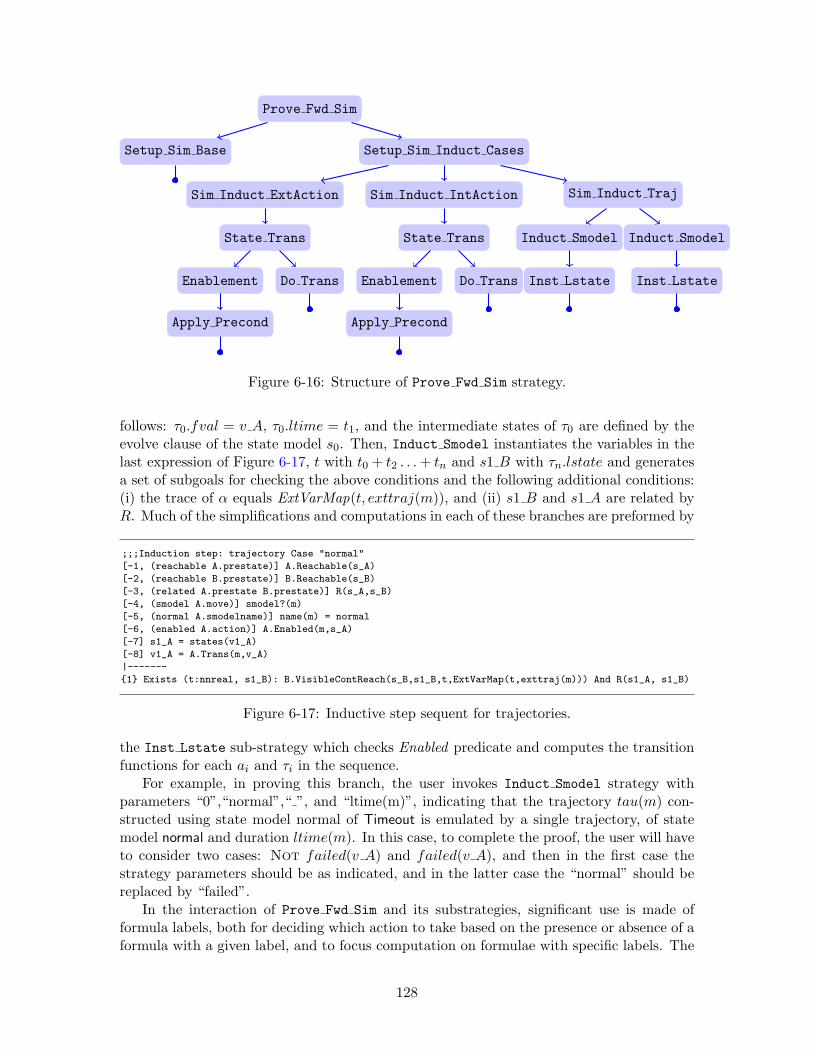
Prove Fwd Sim
Setup Sim Base Setup Sim Induct Cases
Sim Induct ExtAction
State Trans
Enablement
Apply Precond
Do Trans
Sim Induct IntAction
State Trans
Enablement
Apply Precond
Do Trans
Sim Induct Traj
Induct Smodel
Inst Lstate
Induct Smodel
Inst Lstate
Figure 6-16: Structure of Prove Fwd Sim strategy.
follows: τ0.fval = v A, τ0.ltime = t1, and the intermediate states of τ0 are defined by theevolve clause of the state model s0. Then, Induct Smodel instantiates the variables in thelast expression of Figure 6-17, t with t0 + t2 . . .+ tn and s1 B with τn.lstate and generatesa set of subgoals for checking the above conditions and the following additional conditions:(i) the trace of α equals ExtVarMap(t, exttraj(m)), and (ii) s1 B and s1 A are related byR. Much of the simplifications and computations in each of these branches are preformed by
;;;Induction step: trajectory Case "normal"
[-1, (reachable A.prestate)] A.Reachable(s_A)
[-2, (reachable B.prestate)] B.Reachable(s_B)
[-3, (related A.prestate B.prestate)] R(s_A,s_B)
[-4, (smodel A.move)] smodel?(m)
[-5, (normal A.smodelname)] name(m) = normal
[-6, (enabled A.action)] A.Enabled(m,s_A)
[-7] s1_A = states(v1_A)
[-8] v1_A = A.Trans(m,v_A)
|-------
1 Exists (t:nnreal, s1_B): B.VisibleContReach(s_B,s1_B,t,ExtVarMap(t,exttraj(m))) And R(s1_A, s1_B)
Figure 6-17: Inductive step sequent for trajectories.
the Inst Lstate sub-strategy which checks Enabled predicate and computes the transitionfunctions for each ai and τi in the sequence.
For example, in proving this branch, the user invokes Induct Smodel strategy withparameters “0”,“normal”,“ ”, and “ltime(m)”, indicating that the trajectory tau(m) con-structed using state model normal of Timeout is emulated by a single trajectory, of statemodel normal and duration ltime(m). In this case, to complete the proof, the user will haveto consider two cases: Not failed(v A) and failed(v A), and then in the first case thestrategy parameters should be as indicated, and in the latter case the “normal” should bereplaced by “failed”.
In the interaction of Prove Fwd Sim and its substrategies, significant use is made offormula labels, both for deciding which action to take based on the presence or absence of aformula with a given label, and to focus computation on formulae with specific labels. The
128
labels are designed to be informative: for example, the label A.enabled on line 4 of the proofin Figure 6-15 indicates that the enabling condition of the fail action of the automatonA (in this case, Timeout). This is so that when an unresolved subgoal is returned to theuser, its content is as informative as possible. For the same reason, Prove Fwd Sim and itssubstrategies attach comments to any subgoals they create that denote their significance.The comment ;;;Induction step: trajectory Case "normal" that appears on line 2in Figure 6-17 indicates that this subgoal is the subgoal for trajectories of the state modelnormal.
6.4 Discussion of Case Studies
Our approach to mechanizing proofs for the SHIOA framework is to study examples ofSHIOA specifications and their properties and then identify a standard set of proof stepssufficient to mechanize proofs of those properties. To this end, we have targeted invari-ant properties and simulation relations and the outcome has been the strategies such asProve Fwd Sim, Auto Induct, and State Trans. These strategies do not completely elim-inate human intervention but they do eliminate many of the repetitive and tedious stepsthat are necessary for constructing proofs.
Although the translation scheme outlined in Section 6.2 is suitable for any HIOA speci-fication conforming to the assumptions in Section 6.2.1, the current implementation of ourtranslator tool is able to translate the restricted class of HIOA specifications with rectangulardynamics, that is, differential equations with constant right hand sides. As a result, theexamples we have studied thus far all have state models with relatively simple continuousdynamics. Nevertheless, the case studies have interesting data structures and demonstratenon-trivial hybrid behavior. We discuss our experience in applying these strategies to twocase studies.
6.4.1 Failure Detector
The HIOA specification of a simple failure detector system from [KLSV05] was presented inFigure 6-7. The details of the verification of this system appears in [MA05]. The compositespecification consists of (1) a process that sends a message every u1 time units until itfails, (2) a communication channel that delays messages by at most d time units, and (3) adetector process which times out and suspects the sending process to have failed when itdoes not receive a message for u2 = u1 + d time units. We are interested in proving twoproperties for this system, namely, (i) a no false positive property, i.e., whenever the detectorsuspects, the sender is indeed failed, and (ii) a timely detection property, i.e., whenever thesender fails, the detector suspects it within u2 + b time units. Property (i) is a predicate onthe states of the composed system and is stated as an invariant. For describing property (ii),an abstract specification Spec of Timeout is written (shown in Figure 3-7), and then it isproved, using forward simulation, that Timeout implements Spec. The translator generatesPVS theory files for the automaton specifications, the invariants, and the simulation relations(see Figures 6-8, 6-9, 6-12, and 6-6).
We invoke the PVS-prover on these theories to interactively prove the translated lem-mas and theorems. Invariants Inv 1 to Inv 4 of Figure 6-9, are relatively simple and areproved automatically by the Auto Induct strategy. Proofs of invariants Inv 5, Inv 6, andInv 7 require the application of the first four invariants, and consequently, in these casesAuto Induct presents us with a set of subgoals that require manual intervention. At which
129

point, we use a separate strategy called Apply Inv Lemma which introduces invariant lemmaof our choice and instantiates its state appropriately for the current proof context. In mostcases, this completes the proof branch; for some of the branches corresponding to trajectorymoves, further simplifications are necessary.
In the simulation proof of FwdSimThm, each move branch leads to six subgoals corre-sponding to the six high level conjuncts in the simulation relation, but the trivial subgoals(e.g., first two subgoals) are discharged automatically by the Prove Fwd Sim strategy. Theremaining subgoals required the application of previously proved invariants and reasoningabout inequalities involving real expressions for which we also use the strategies in theManip [MM01] and the Field [Vit02] packages.
6.4.2 Two-Task Race
In this case study we applied our strategies to prove time bounds through a forward simu-lation in the two process race system described in [Lyn96b]. The automaton TwoTaskRace(see Figure 6-18) models two processes running in parallel. The main process triggers anaction once every t time, where t is between a1 and a2. The second process produces a setaction within the time interval [b1, b2]. The main process triggers increment actions, incre-menting a count, until the set action occurs. After set, the main process triggers decrementactions, which decrements a count. When the count reaches 0 then the main process triggersa report action, which indicates the end of execution. The property that we investigateis the upper and lower time bounds on the occurrence of report action. The details of thetranslation and verification of the system appears in [LKLM05].
Here we focus to the upper time bound which is b2 + a2 + b2a2a1
. The intuition behindthis bound as follows: in order to maximize the value of the counter until set occurs, themain process should increment count every a1 time. Thus, the value of count when the setaction occurs is b2/a1. Thereafter, the maximum time taken to decrement count down tozero is a2b2/a1. The latest time when the set action occurs is b2, and therefore the uppertime bound for report is a2 + b2 + a2b2/a1.
This time bounds on report are specified as a simple abstract automaton TwoTaskRaceSpecwhich triggers a report action within the above time bound. A forward simulation relationof Figure 6-19 is used to prove that TwoTaskRace implements TwoTaskRaceSpec. This sim-ulation relation is more complex than that for the Timeout example because the relationbetween the states differs depending on whether or not the set action has occurred. Theoccurrence of the set action set the flag variable to true. For example, lines 16–17 relatethe deadline variable first report of TwoTaskRaceSpec to the deadline variable first setand the counter of TwoTaskRace, for the case where the flag has been set. While a differentrelation is stated in lines 21–23 for the case where the flag has not been set.
The structure of the proof is similar to that for Timeout and Spec and so Prove Fwd Simstrategy successfully breaks up the simulation proof into subgoals for the individual ac-tions and trajectories. Applying Sim Induct ExtAction, Sim Induct IntAction , andSim Induct Traj with proper arguments instantiates and simplifies the move branches.
In our case studies, the proofs translated theories constructed using our strategies require70% or fewer proof steps than those constructed using raw PVS proof commands. Thiscomparison, however, may not be completely fair because our translation is specificallygeared toward making the strategies work efficiently, and it adds extra structures in thegenerated PVS theories that eliminate the generation of some type-correctness-related sub-
130
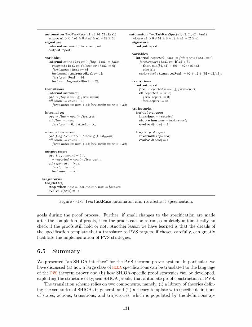
automaton TwoTaskRace(a1, a2, b1, b2 : Real)where a1 > 0 ∧ b1 ≥ 0 ∧ a2 ≥ a1 ∧ b2 ≥ b1
signatureinternal increment, decrement, setoutput report
variablesinternal count : Int := 0; flag : Bool := false;reported : Bool := false;now : Real := 0;first main : Real := a1;last main : AugmentedReal := a2;first set : Real := b1;last set : AugmentedReal := b2;
transitionsinternal incrementpre ¬ flag ∧now ≥ first main;eff count := count+ 1;first main := now + a1; last main := now + a2;
internal setpre ¬ flag ∧now ≥ first set;eff flag := true;first set := 0; last set := ∞;
internal decrementpre flag ∧ count > 0 ∧now ≥ firstmain;eff count := count− 1;first main := now + a1; last main := now + a2;
output reportpre flag ∧ count = 0 ∧¬ reported ∧now ≥ firstmain;
eff reported := true;firstmain := 0;last main := ∞;
trajectoriestrajdef traj
stop when now = last main ∨now = last set;evolve d(now) = 1;
automaton TwoTaskRaceSpec(a1, a2, b1, b2 : Real)where a1 > 0 ∧ b1 ≥ 0 ∧ a2 ≥ a1 ∧ b2 ≥ b1signature
output report
variablesinternal reported : Bool := f alse;now : Real := 0;first report : Real := if a2 < b1
then min(b1, a1) + (b1− a2) ∗ a1/a2else a1;
last report : AugmentedReal := b2 + a2 + (b2 ∗ a2/a1);
transitionsoutput report
pre ¬ reported ∧now ≥ firstreport;eff reported := true;first report := 0;last report := ∞;
trajectoriestrajdef pre report
invariant ¬ reported;stop when now = last report;evolve d(now) = 1;
trajdef post reportinvariant reported;evolve d(now) = 1;
Figure 6-18: TwoTaskRace automaton and its abstract specification.
goals during the proof process. Further, if small changes to the specification are madeafter the completion of proofs, then the proofs can be re-run, completely automatically, tocheck if the proofs still hold or not. Another lesson we have learned is that the details ofthe specification template that a translator to PVS targets, if chosen carefully, can greatlyfacilitate the implementation of PVS strategies.
6.5 Summary
We presented “an SHIOA interface” for the PVS theorem prover system. In particular, wehave discussed (a) how a large class of HIOA specifications can be translated to the languageof the PVS theorem prover and (b) how SHIOA-specific proof strategies can be developed,exploiting the structure of typical SHIOA proofs, that automate proof construction in PVS.
The translation scheme relies on two components, namely, (i) a library of theories defin-ing the semantics of SHIOAs in general, and (ii) a theory template with specific definitionsof states, actions, transitions, and trajectories, which is populated by the definitions ap-
131
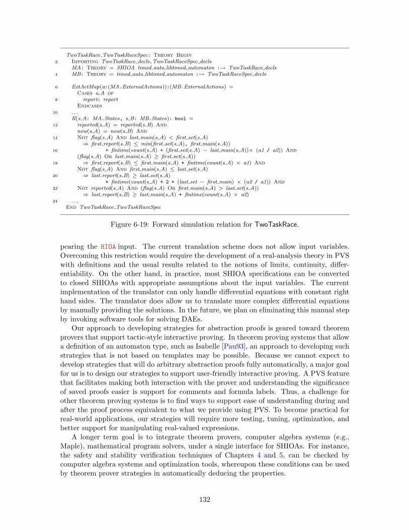
TwoTaskRace TwoTaskRaceSpec: Theory Begin2 Importing TwoTaskRace decls,TwoTaskRaceSpec decls
MA: Theory = SHIOA timed auto libtimed automaton :→ TwoTaskRace decls4 MB: Theory = timed auto libtimed automaton :→ TwoTaskRaceSpec decls
6 ExtActMap(a:(MA.ExternalActions)):(MB.ExternalActions) =Cases a A of
8 report: reportEndcases
10 . . .R(s A: MA.States, s B: MB.States): bool =
12 reported(s A) = reported(s B) Andnow(s A) = now(s B) And
14 Not flag(s A) And last main(s A) < first set(s A)⇒ first report(s B) ≤ min(first set(s A), first main(s A))
16 + fintime(count(s A) + (first set(s A) − last main(s A))× (a1 / a2)) And(flag(s A) Or last main(s A) ≥ first set(s A))
18 ⇒ first report(s B) ≤ first main(s A) + fintime(count(s A) × a1) AndNot flag(s A) And first main(s A) ≤ last set(s A)
20 ⇒ last report(s B) ≥ last set(s A)+ fintime(count(s A) + 2 + (last set − first main) × (a2 / a1)) And
22 Not reported(s A) And (flag(s A) Or first main(s A) > last set(s A))⇒ last report(s B) ≥ last main(s A) + fintime(count(s A) × a2)
24 . . .End TwoTaskRace TwoTaskRaceSpec
Figure 6-19: Forward simulation relation for TwoTaskRace.
pearing the HIOA input. The current translation scheme does not allow input variables.Overcoming this restriction would require the development of a real-analysis theory in PVSwith definitions and the usual results related to the notions of limits, continuity, differ-entiability. On the other hand, in practice, most SHIOA specifications can be convertedto closed SHIOAs with appropriate assumptions about the input variables. The currentimplementation of the translator can only handle differential equations with constant righthand sides. The translator does allow us to translate more complex differential equationsby manually providing the solutions. In the future, we plan on eliminating this manual stepby invoking software tools for solving DAEs.
Our approach to developing strategies for abstraction proofs is geared toward theoremprovers that support tactic-style interactive proving. In theorem proving systems that allowa definition of an automaton type, such as Isabelle [Pau93], an approach to developing suchstrategies that is not based on templates may be possible. Because we cannot expect todevelop strategies that will do arbitrary abstraction proofs fully automatically, a major goalfor us is to design our strategies to support user-friendly interactive proving. A PVS featurethat facilitates making both interaction with the prover and understanding the significanceof saved proofs easier is support for comments and formula labels. Thus, a challenge forother theorem proving systems is to find ways to support ease of understanding during andafter the proof process equivalent to what we provide using PVS. To become practical forreal-world applications, our strategies will require more testing, tuning, optimization, andbetter support for manipulating real-valued expressions.
A longer term goal is to integrate theorem provers, computer algebra systems (e.g.,Maple), mathematical program solvers, under a single interface for SHIOAs. For instance,the safety and stability verification techniques of Chapters 4 and 5, can be checked bycomputer algebra systems and optimization tools, whereupon these conditions can be usedby theorem prover strategies in automatically deducing the properties.
132

Part II
Probabilistic Hybrid Systems
133

Chapter 7
Probabilistic State Machines
Structured Hybrid I/O Automata (SHIOAs) of Part I model system uncertainties as non-deterministic choices. Nondeterminism describes uncertainty as a set of possible choices,but does not capture the probability of individual choices. Incorporating probabilities in thehybrid system framework gives us a richer language to construct models with. In additionto the types of properties we studied in Part I, with probabilistic models we can begin tostate and prove quantitative properties, such as probability of hitting unsafe states andexpected time of stabilization. Developing semantics and verification techniques for modelsthat combine nondeterminism, probabilities, and continuous evolution poses two key chal-lenges, namely, (i) reconciling the interaction between probabilistic and nondeterministicchoices, and (ii) ensuring measurability of all reasonable sets of executions. We refer thereader back to Section 1.3.1 for an informal discussion of these two issues. In this chapterwe make certain design decisions to solve these problems and present them in the formof the Probabilistic Timed I/O Automata (PTIOA) framework. A transition of a PTIOAcan be nondeterministic and probabilistic; continuous evolution is non-probabilistic; andconcurrently executing automata communicate through shared actions. We develop thetrace-based semantics for PTIOAs which involves measure-theoretic constructions on thespace of executions of the automata. We introduce a new notion of external behavior andimplementation for PTIOAs and show that PTIOAs have simple substitutivity properties.In Chapter 8, we present techniques for verifying approximate implementation relations fora restricted class of PTIOAs.
7.1 An Overview
Automata with probabilistic transitions are useful for modeling systems that interact withenvironments with stochastic description of uncertainties. Examples include Gaussian chan-nel delays, stochastic noise in sensors, processor failure probabilities, and also randomiza-tion in algorithms. Pure nondeterminism, on the other hand, is necessary for construct-ing (a) implementation-free, abstract models that are underspecified, and (b) models witharbitrary interleaving of concurrently executing processes. For a detailed discussion onthe need for nondeterminism in probabilistic automata we refer the reader to Chapter 4of [Her02] and the introduction of [dA97]. The interplay between probability and non-determinism makes it challenging to develop semantics for automaton models that haveboth [Seg95b, MOW04, Che06, CCK+06b]. Introduction of continuous state spaces and dis-tributions adds another layer of complexity to the problem [CSKN05, vBMOW05, DDLP05].
134

The PTIOA framework presented here addresses some these challenges. A PTIOA canmake nondeterministic and probabilistic choices, its continuous evolution is not stochas-tic, and sets of PTIOAs communicate through shared actions. PTIOAs generalize sev-eral existing models, including Timed I/O Automata [KLSV05], Probabilistic I/O Au-tomata [Seg95b, CCK+06b] and its timed extension presented in [Seg95b], and discretestate Markov Decision Processes [dA97, BCG06, KNSW04, HKNP06].
In Section 7.2, we recall some standard notions from measure theory. In Section 7.3 wepresent the non-probabilistic semantics for PTIOAs which closely parallels the semanticsof SHIOAs with one major difference: PTIOAs do not have input/output variables. Thisimplies that a trace of a PTIOA contains information about the occurrence of input/outputactions and the duration of time that elapses between them, but not about evolution ofvariables over that time.
In Section 7.4 we develop the probabilistic semantics for PTIOAs. In order to ensurethat all reasonable sets of executions are measurable we impose the following measurabilityconditions on a PTIOA A which has measurable space (Q,FQ) as its state space: M1 forany action, the set of states in which the action is enabled a FQ-measurable, and M2 formeasurable subsets R ⊆ R≥0, Y ⊆ Q, the set of states from which there exists a trajectorywith length in R and final state in Y , is FQ-measurable. In order to define a probabilitydistribution over the set of executions of a PTIOA A, the nondeterministic choices in A haveto be resolved first. Nondeterminism comes from two sources: (a) external nondeterminism:choice of one automaton which makes the next move from a set of interacting automata,and (b) internal nondeterminism: choice of one move (transition or trajectory) from a setof possible moves of an automaton, We proceed by working with a restricted model, namely,Task-Structured Deterministic PTIOA (task-DPTIOA), that has limited internal nondeter-minism, and then develop the semantics for general PTIOAs in Section 7.6. For resolvingexternal nondeterminism we rely on the task structure and task schedules, similar to thoseintroduced in [CCK+06b]. The task-structure ensures that a task uniquely determines antask-DPTIOA which gets to make the next move. The sequence of tasks is specified by atask schedule. Combining a task schedule with a task-DPTIOA A gives rise to a probabilisticexecution—a probability measure over the set of executions of A.
The construction of probability measure over executions of task-DPTIOAs is similar inspirit to that in the case of Stochastic Transition Systems (STS) of Cattani et al. [CSKN05].However, a STS does not have notions of time or trajectories and this leads to very differ-ent notions of observable behavior or traces (see Section 7.4.3 for details). In particular,this issue surfaces as we define a distribution over traces corresponding to a probabilisticexecution.
In Section 7.5, we use a simple, but intuitive notion of external behavior for task-DPTIOAs: for a given automaton A, its external behavior is a function that maps eachclosing environment E of A to the set of all possible trace distributions of the composition ofA and E . We show that task-DPTIOAs are substitutive with respect to the implementationrelation defined in terms of the above notion of external behavior. Indeed, considering closedautomata and using this functional definition of external behavior lets us circumvent some ofthe difficulties that underlie compositionality in the probabilistic setting. However, viewingexternal behavior as a mapping from environments as opposed to a set of trace distribu-tions is natural in many applications, including analysis of security protocols [CCK+06c].Section 7.7 presents an extension of the HIOA language for specifying PTIOAs and examplesillustrating the key notions introduced in the chapter.
135
7.2 Preliminaries
Deterministic Sets of Trajectories. The notations for sets, functions, variables, andtrajectories from Section 2.1 of Part I have the same meanings unless stated otherwise. Weassociate with the time axis T = R≥0 ∪ ∞ the Euclidean topology with a point at ∞.Let X be a set of variables. The set of all valuations for the variables in X is denotedby val(X). Given a set of trajectories T for X, we denote the subset of T starting fromx ∈ val(X), by T (x). A set of trajectories T for X is deterministic if for all x ∈ val(X),for any two trajectories τ1, τ2 ∈ T (x) either τ1 is a prefix of τ2 or τ2 is a prefix of τ1. If Tis deterministic then for any x ∈ val(X), (T (x),≤) is a total order.
As max(x) is required to be a closed trajectory,max(x).ltime and max(x).lval are welldefined.
Measurability and Measures. We follow the standard notations as found in any textbook on measure theory, as for instance [Dud89]. A measurable space is denoted by (S,FS),where S is a set and FS is a σ-algebra over S. FS is closed under countable union andcomplementation and its members are called measurable sets. Given a topological space(S,T ), there exists a smallest σ-algebra containing T and it is called the Borel σ-algebra.Whenever the sets R,R≥0 and T are viewed as measurable spaces, it is assumed that theyare equipped with their usual Borel σ-algebras.
The product of two measurable spaces (S1,FS1) and (S2,FS2) is defined as the measur-able space (S1 × S2,FS1 ⊗ FS2), where FS1 ⊗ FS2 is the smallest σ-algebra generated bysets of the form A×B = (s1, s2) | s1 ∈ A, y ∈ B, for all A ∈ FS1 , B ∈ FS2 .
A measure over (S,FS) is a function µ : FS → R≥0, such that µ(∅) = 0 and for everycountable collection of disjoint sets Sii∈I in FS , µ(
⊎i∈I Si) =
∑i∈I µ(Si). Recall that⊎
i∈I Si denotes the union of a collection Sii∈I of pairwise disjoint sets. A probabilitymeasure (resp. sub-probability measure) over (S,FS) is a measure µ such that µ(S) = 1(µ(S) ≤ 1). The set of probability measures and the set of sub-probability measures over(S,FS) is denoted by P(S,FS) and SP(S,FS). A particular family of probability measuresis the Dirac measures: given a measurable space (S,FS) where singleton sets are measurableand s ∈ S, the Dirac measure at s, denoted by δs, is defined as δs(A) = 1 if s ∈ A, δs(A) = 0otherwise.
A function f : (S1,FS1) → (S2,FS2) is said to be measurable if f−1(E) ∈ FS1 for everyE ∈ FS2 . The indicator function of a set A ⊆ S1, is defined as IA(s) = 1 if s ∈ A, and 0otherwise. If A is a measurable set, it is easy to check that IA is a measurable function.If f : (S1,FS1) → (S2,FS2) is a measurable function, and µ is a measure on S1, then theimage measure of µ under f is a measure ϕ on Y defined as ϕ(E) = µ(f−1(E)), for eachE ∈ FS2 .
Integration. A simple function f on a measurable space (S,FS) is a function whose rangeconsists of only finitely many points in [0,∞). If c1, . . . , cn are distinct values of a simplefunction f , and if we set Ci = s | f(s) = ci, then f(s) =
∑ni=1 ciICi(s), where ICi
is the indicator function of Ci. It is clear that f is measurable if and only if Ci ∈ FS ,for each i ∈ 1, . . . , n. If f : S → R≥0 is a simple measurable function of the formf =
∑ni=1 ciICi(s), where c1, . . . , cn are distinct values of f , and if E ∈ FS , we define∫
Efdµ =
n∑i=1
ciµ(Ci ∩ E).
136
If f : S → R≥0 is measurable and E ∈ FS , the Lebesgue integral of f over E is defined as∫Efdµ
∆= sup0≤f≤f
∫Efdµ,
the supremum being taken over all simple measurable functions f that are less than f .
Semi-Rings. A collection C of subsets of S, is a semi-ring if (1) the sets S and ∅ arein C , (2) for any A,B ∈ C , A ∩ B ∈ C , and (3) for any A,B ∈ C , there exists a finitecollection of disjoint sets Cini=1 in C such that A \ B =
⋃ni=1Ci. It is well known (see,
e.g. [Dud89]) that a measure µ defined over a semi-ring C can be uniquely extended to ameasure over the σ-algebra generated by C by defining µ(∪ni=1Ci) =
∑ni=1 µ(Ci). We will
use the following theorem to constructing measures of the space of executions of automata:
Theorem 7.1. A probability measure defined over a semi-ring C can be uniquely extendedto a probability measure over the σ-algebra generated by C .
In constructing measures over the space of executions of a PTIOA, we have to integrate overthe space of probability distributions over sets, namely the state space Q, and therefore,we need to define a σ-algebra over P(Q,FQ). For this, we use the following constructiondue to Giry [Gir81]: for each A ∈ FQ, let the function pA : P(Q,FQ) → [0, 1] be definedas pA(µ) = µ(A). The σ-algebra on P(Q,FQ), then is the smallest σ-algebra such that allpA’s are measurable.
7.3 Task-Deterministic Probabilistic Timed I/O Automata
In this section we introduce Task-Deterministic Probabilistic Timed Input/Output Automata(Task DPTIOAs) and present definitions and results regarding the non-probabilistic aspectsof their behavior.
7.3.1 Definition of Task DPTIOAs
We present the definition of Task DPTIOAs in two parts. First we define ProbabilisticTimed I/O Automata (PTIOAs) and then we impose several assumptions that restrict thenondeterminism in a PTIOA to obtain the task DPTIOA model.
Definition 7.1. A Probabilistic Timed I/O Automaton A = (X, (Q,FQ), x, A,D, T ), where:
(a) X is a set of internal or state variables.
(b) Q ⊆ val(X) is a set of states, (Q,FQ) is a measurable space called the state space,and x ∈ Q is the start state.
(c) A is a countable set of actions, partitioned into internal H, input I and output Oactions. L = O ∪ H is the set of local actions and E = O ∪ I is the set of externalactions.
(d) D ⊆ Q×A×P(Q,FQ) is the set of probabilistic transitions. If (x, a, µ) is an elementof D, we write x a→ µ and action a is said to be enabled at x. The set of states inwhich action a is enabled is denoted by Ea. For B ⊆ A, we define EB to be ∪a∈BEa.The set of actions enabled at x is denoted by enabled(x). If a single action a ∈ B ⊆
137
is enabled at x and x a→ µ, then this µ is denoted by µx,B. If B is a singleton set athen we drop the set notation and write µx,a.
(e) T is a set of trajectories for Q that is (i) deterministic, (ii) closed under prefix, suffix,concatenation, and (iii) contains ℘(x) for every x ∈ Q. For R ⊆ R≥0 and P ⊆ Q, wedefine ER,P to be the set of states x ∈ Q | ∃ closed τ ∈ T (x), τ.ltime ∈ R ∧ τ.lstate ∈P.
In addition A must satisfy the following conditions:
E1 (Input action enabled) For every input action a ∈ I and for every statex ∈ Q, a is enabled at x.
E2 (Time passage enabled) For every state x ∈ Q, there exists τ ∈ T (x) suchthat either τ.ltime = ∞ or τ is closed and some a ∈ L is enabled in τ.lstate.
M1 (Transitions measurability) For every a ∈ L, Ea is measurable.
M2 (Trajectory measurability) For measurable sets R ⊆ R≥0, Y ∈ FQ, ER,Y ismeasurable.
P1 (Progressive) A never generates infinitely many locally controlled actionswithin a finite time interval.
Notations. A PTIOA which does not necessarily satisfy axioms M1 and M2 is calleda pre-PTIOA. A pre-PTIOA is closed if its set of input actions is empty. We denote thecomponents of a pre-PTIOA A by XA, QA, xA,DA, TA etc., and the components of a pre-PTIOA Ai by Xi, Qi,xi,Di, etc. The special sets of states of pre-PTIOA A that we definedabove, are denoted by Ea,A, ER,Y,A, etc., and those of pre-PTIOA Ai by Ea,i, ER,Y,i, etc.
The axioms E1 and E2 are identical to the standard non-blocking axiom of SHIOAs. SincePTIOAs do not have input variables, here the input trajectory enabled axiom takes the formof the time-passage-enabled axiom E2. Axioms M1 and M2 are used later to constructa measurable space over the set of executions of A and to assign probabilities measuresto certain measurable sets of executions. M1 states that for any local action a, the set ofstates of A in which a is enabled is a measurable set, and M2 states that for measurablesubsets R ⊆ R≥0, Y ⊆ Q, the set of states from which there exits a closed trajectory withlength in R and final state in Y , is a measurable set. E1 and M1 together imply that EBis a measurable set for any set of actions B ⊆ A. The progressive axiom P1 is a naturalassumption for timed automata (see, Page 75 of [KLSV05]). The formal meaning of P1 isgiven shortly after we define executions of A.
A few remarks comparing this definition with that of a Structured Hybrid I/O Automa-ton of Part I:
(1) The measurability requirement on Q is quite weak; most state spaces that we typicallyencounter in applications are measurable.
(2) Unlike SHIOAs, PTIOAs do not have input or output variables, because we assume thatPTIOAs communicate through shared actions only and not through shared variables.Extending the results presented here to a model with external variables is a directionof future research.
(3) For clarity of exposition, it is assumed that PTIOAs start from a single start state xand that the set of actions A is countable; correctness of our results does not depend
138
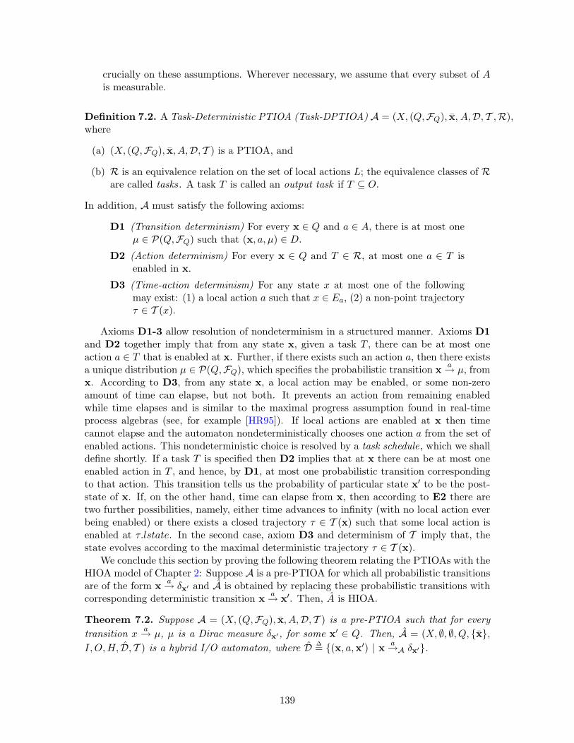
crucially on these assumptions. Wherever necessary, we assume that every subset of Ais measurable.
Definition 7.2. A Task-Deterministic PTIOA (Task-DPTIOA) A = (X, (Q,FQ), x, A,D, T ,R),where
(a) (X, (Q,FQ), x, A,D, T ) is a PTIOA, and
(b) R is an equivalence relation on the set of local actions L; the equivalence classes of Rare called tasks. A task T is called an output task if T ⊆ O.
In addition, A must satisfy the following axioms:
D1 (Transition determinism) For every x ∈ Q and a ∈ A, there is at most oneµ ∈ P(Q,FQ) such that (x, a, µ) ∈ D.
D2 (Action determinism) For every x ∈ Q and T ∈ R, at most one a ∈ T isenabled in x.
D3 (Time-action determinism) For any state x at most one of the followingmay exist: (1) a local action a such that x ∈ Ea, (2) a non-point trajectoryτ ∈ T (x).
Axioms D1-3 allow resolution of nondeterminism in a structured manner. Axioms D1and D2 together imply that from any state x, given a task T , there can be at most oneaction a ∈ T that is enabled at x. Further, if there exists such an action a, then there existsa unique distribution µ ∈ P(Q,FQ), which specifies the probabilistic transition x a→ µ, fromx. According to D3, from any state x, a local action may be enabled, or some non-zeroamount of time can elapse, but not both. It prevents an action from remaining enabledwhile time elapses and is similar to the maximal progress assumption found in real-timeprocess algebras (see, for example [HR95]). If local actions are enabled at x then timecannot elapse and the automaton nondeterministically chooses one action a from the set ofenabled actions. This nondeterministic choice is resolved by a task schedule, which we shalldefine shortly. If a task T is specified then D2 implies that at x there can be at most oneenabled action in T , and hence, by D1, at most one probabilistic transition correspondingto that action. This transition tells us the probability of particular state x′ to be the post-state of x. If, on the other hand, time can elapse from x, then according to E2 there aretwo further possibilities, namely, either time advances to infinity (with no local action everbeing enabled) or there exists a closed trajectory τ ∈ T (x) such that some local action isenabled at τ.lstate. In the second case, axiom D3 and determinism of T imply that, thestate evolves according to the maximal deterministic trajectory τ ∈ T (x).
We conclude this section by proving the following theorem relating the PTIOAs with theHIOA model of Chapter 2: Suppose A is a pre-PTIOA for which all probabilistic transitionsare of the form x a→ δx′ and A is obtained by replacing these probabilistic transitions withcorresponding deterministic transition x a→ x′. Then, A is HIOA.
Theorem 7.2. Suppose A = (X, (Q,FQ), x, A,D, T ) is a pre-PTIOA such that for everytransition x
a→ µ, µ is a Dirac measure δx′, for some x′ ∈ Q. Then, A = (X, ∅, ∅, Q, x,I, O,H, D, T ) is a hybrid I/O automaton, where D ∆= (x, a,x′) | x a→A δx′.
139
Proof. All the components of A satisfy the type requirements in the definition of a HIOA.In particular, D is flattened to be a subset of Q×A×Q. The set of trajectories of A satisfiesT1-3 from the definition of T . This establishes that A is a pre-HIOA. Since A does not haveany input variables, checking that it is input-trajectory-enabled is tantamount to checkingthat it is time-passage-enabled, which is implied by bf E2 of A.
7.3.2 Executions and Traces
Execution fragments and executions of a PTIOA A are defined in the same way as in thecase of HA (see, Section 2.2.2). We remind the reader that an execution fragment of is analternating sequence of actions and trajectories α = τ0a1τ1a2 . . ., where each τi ∈ T , ai ∈ Aand ai is enabled at τi−1.lstate. The first state of an execution fragment α, α.fstate, isτ0.fstate. An execution fragment α is an execution of A if α.fstate = x. The length of afinite execution fragment α is the number of trajectories in α. An execution fragment isclosed if it is a finite sequence and the last trajectory is closed. Proposition 7.3 follows fromaxiom D3.
Proposition 7.3. In any execution fragment of a closed PTIOA all trajectories, exceptpossibly the last trajectory (of a finite fragment) are maximal.
Proof. Suppose, for the sake of contradiction, the proposition is false. That is, there existsa non-final, non-maximal trajectory τ in the execution fragment α. Since τ is not maximal,there exists a non point trajectory τ ′, such that τ ′ is enabled at τ.lstate. Since τ is non-final,there exists an action ai+1 ∈ A, that is enabled at τ.lstate. This contradicts D3 at τ.lstate.
The trace of an execution α represents its externally visible part. Unlike SHIOAs, aPTIOA does not have external variables. Hence, the externally visible part of any trajectoryτ of a PTIOA is simply a mapping from dom(τ) to the empty set of variables. Formally,the trace of an execution α, denoted by trace(α), is the (E, ∅)-restriction of α. The onlyinformation that is conveyed by the externally visible part of a trajectory τ is dom(τ), andhence, the information in the trace of an execution fragment is the external actions andduration of the intervening time intervals. For the development of probabilistic semanticsfor task-DPTIOAs it will be necessary for the trace function to be measurable; we shallprove this result in Section 7.4.3.
It is worth comparing this definition of a trace of a PTIOA with that in other probabilis-tic transition systems that do not have special semantics for modeling time and trajectories.For example, in Stochastic Transition System (STS) of [CSKN05], a trace is obtained bysimply removing the internal (invisible) actions and states from an execution. In such mod-els, one obvious approach for modeling time passage is to treat a transition labeled by areal number r as a time passage action of duration r. So, an execution is a sequence forthe form q0 r0 q1 a1 q2 r1 q3 a2 q4, where the q′is are states, a1 is an internal action, a2
is an external actions, and r0, r1 ∈ R≥0 are internal actions which model the passage oftime. The trace of an STS contains information about the point of occurrence of internalactions over an interval of time. For example, the trace of the above execution is r0r1a2,which tells us that some internal action occurred between r0 and r1. And this makes itrelatively straightforward to show that the trace function is measurable. In PTIOAs, thetrace of an execution τ0a1τ1a2τ2, where a1 is an internal action and a2 is an external action,
140

equals ((τ0 _ τ1) ↓ ∅)a2(τ2 ↓ ∅). Concatenating τ0 and τ1 hides information about thetime of occurrence of internal actions a1. Consequently, this “information loss” makes theproof of measurability of the trace function more complicated in PTIOAs, compared to thecorresponding proof in the STS setting.
We denote the set of execution fragments, the set of executions, and the set of tracesof PTIOA A by FragsA, ExecsA and TracesA. The set of finite fragments, finite executionsand finite traces are denoted by Frags∗A, Execs∗A and Traces∗A. Having defined traces andexecutions, we can now state the meaning of axiom P1 formally. This axiom asserts thatover any execution fragment α, if α.ltime is finite then α can have only a finite number oflocally controlled actions.
7.3.3 Composition of Task-DPTIOAs
The composition operation enables us to construct a PTIOAs representing a complex systemfrom two interacting PTIOAs by identifying their external actions that have the samenames. PTIOAs do not have external (input/output) variables and component automatacommunicate through external actions only.
Definition 7.3. Pre-PTIOAs A1 and A2 are compatible if X1∩X2 = H1∩A2 = H2∩A1 =O1 ∩ O2 = ∅. If A1 and A2 are compatible pre-PTIOAs then their composition A1||A2, isdefined to be A ∆= (X, (Q,FQ), x, A,D, T ), where:
(a) X = X1 ∪X2,
(b) (Q,FQ) = (Q1 ×Q2,FQ1 ⊗FQ2), and x = (x1, x2),
(c) A = A1 ∪A2, I = (I1 ∪ I2) \ (O1 ∪O2), O = O1 ∪O2, and H = H1 ∪H2,
(d) D ⊆ Q×A×P(Q,FQ) is the set of triples ((x1,x2), a, µ1⊗µ2) such that for i ∈ 1, 2if a ∈ Ai then (xi, a, µi) ∈ Di, otherwise µi = δxi ,
(e) T = τ ∈ trajs(X) | τ ↓ Xi ∈ Ti, i ∈ 1, 2, and
We show that the class of pre-PTIOAs are closed under the composition operator.
Theorem 7.4. If A1,A2 are compatible pre-PTIOAs then A = A1||A2 is a pre-PTIOA.
Proof. Parts (a), (b), (c), (d), and (f) of Definition 7.3 match with the correspondingparts of Definition 7.1. We check that the set T of trajectories of A satisfy the necessaryproperties stated in Part (e) of Definition 7.1. The fact that T is closed under prefix, suffix,concatenation follow from Definition 7.3. It is also easy to check that ℘(x) ∈ T , for everyx ∈ Q. Next, we show that T is deterministic. Consider two distinct trajectories τ, τ ′ ∈T (x), for some x ∈ Q with τ ⊆ τ ′. Since (τ ↓ Xi), (τ ′ ↓ Xi) ∈ Ti(x d Xi), for i ∈ 1, 2and Ti is a deterministic set of trajectories for Xi, it follows that (τ ↓ Xi) ≤ (τ ′ ↓ Xi).Combining this result for 1 and 2, we get τ ≤ τ ′.
The fact that A satisfies axioms E1 and E2 follow from Theorem 7.2 of [KLSV05], andthat it satisfies P1 follows from Theorem 7.12 of [KLSV05].
Lemma 7.5. If A1,A2 are compatible pre-PTIOAs and they individually satisfy M1 thenA = A1||A2 is a pre-PTIOA satisfying M1.
141

Proof. From theorem 7.4, we know that A is a pre-PTIOA. We have to show that for anylocal action a ∈ L, the set of states Ea is FX1 ⊗ FX2-measurable. Suppose a is a localaction of A1, and let E1
a ⊆ X1 be the set of states of A1 where a is enabled. The set ofstates of A where a is enabled is Ea = E1
a × X2. A1 satisfies M1, therefore E1a ∈ FX1
and Ea = E1a × X2 ∈ FX1 ⊗ FX2 . The case for a ∈ L, where a is a local action of A2 is
symmetric.
Theorem 7.6. If A1,A2 are compatible PTIOAs and A = A1||A2 satisfies M2 then A isa PTIOA.
Proof. Follows from Lemma 7.5 and the assumption that A satisfies M2.
Definition 7.4. Task-DPTIOAs A1 = (H1,R1) and A2 = (H2,R2) are compatible if theunderlying PTIOAsH1 andH2 are compatible. If A1 and A2 are compatible task-DPTIOAsthen their composition A1||A2, is defined to be A ∆= (H,R), where: (a) H = H1||H2 and(b) R = R1 ∪R2.
Theorem 7.7. If A1,A2 are compatible task-DPTIOAs and A = A1||A2 satisfies M2 thenA is a task-DPTIOA.
Proof. Follows from Theorem 7.6 that A is a PTIOA. Note that R1 ∪R2 is an equivalencerelation because compatibility ofA1 andA2 ensures disjoint sets of locally controlled actions.
We check that A satisfies axioms D1-3. Transition determinism D1 follows immediatelybecause the sets of states are disjoint, and A1,A2 satisfy D1 individually. It is also easy tocheck that action determinism D2 is preserved under composition. Finally, we check thatA satisfies time-action determinism D3. Suppose some local action a ∈ L is enabled at agiven state x. Let us assume without loss of generality that a ∈ L1 and a /∈ L2. Then a isenabled at x d X1 and since A satisfies D3, there does not exist any non-point trajectoryin T1 (and therefore in T ) that starts from x d X1. Likewise, if there exists a non-pointtrajectory starting from x, then no local action is enabled at x d X1 or at x d X2.
We conclude this section with a projection lemma for composed PTIOAs analogous toLemma 2.2 for non-probabilistic hybrid automata.
Theorem 7.8. Suppose A1 and A2 are pre-PTIOAs and A = A1||A2. If α is an executionof A1||A2, then for i ∈ 1, 2, α d (Xi, Ai) is an execution for Ai.
Proof. Let α be any execution of A. The proof is by induction on the length of α. Theinteresting case arises when α = α′a1τ , where τ is a trajectory T , and a1 ∈ A1 \A2, and wehave to show that α d (A2, X2) is an execution of A2. Since a1 ∈ A1 \ A2, α d (A2, X2) =α′ d (A2, X2) _ (τ ↓ X2). From Definition 7.3 we have α′.lstate d X2 = (τ ↓ X2).fstate,therefore, indeed (α′ _ τ) d (A2, X2) is an execution of A2.
7.4 Probabilistic Semantics for Task-DPTIOAs
In the previous section, we presented the basic definitions and results concerning non-probabilistic behavior of PTIOAs. The set of executions and traces of a PTIOA A corre-spond to all possible behaviors and visible behaviors of A. As we saw, these non-probabilisticnotions are closely related to the corresponding notions for SHIOAs presented in Chapter 2.
142

The PTIOA framework, of course, is distinct because here in addition to specifying the setof possible transitions, the models also specify the probability of those transitions. Thus,in the PTIOA framework, we can describe and reason about not just the set of possiblebehaviors, but also the set of probability distributions over all (visible) behaviors. In thissections, we develop the mathematical machinery for such probabilistic reasoning.
In order to construct a probability measure over the set of executions of a given PTIOAA, we have to first define the measurable sets in ExecsA. In the standard approach forprobabilistic automata with discrete state spaces [Seg95b, CCK+06b, KNSW04] one definesthe σ-algebra as the collection of sets of the form Cα := α′ | α is a prefix of α′. Onethen defines the probability of each Cα as the product of the probabilities of the transitionsequence in α. It is well known (see, e.g., generalization of Markov processes in [Doo53]) thatthis approach does not work when the transitions give continuous probability distributions,as in the case of PTIOAs. This is because the probability of occurrence of any particularfinite sequence of transitions is typically 0. Instead of considering a set of executions thatextend a single prefix, we consider a set containing executions that extend any prefix froma “cylinder” or base of prefixes. A similar technique of constructing the measurable space ofexecutions using cylinders has been previously employed in the setting of STS with generalstate spaces and actions [CSKN05].
7.4.1 Semi-ring on Executions and Traces
Definition 7.5. A base is a finite sequence of the form
Λ = Q0 R0 Q′0 A1 Q1 R1 Q
′1 A2 Q2 R2 . . . Q
′m−1 Am Qm Rm Q′m,
where for every i ∈ 0, . . . ,m, Qi, Q′i ∈ FQ, Ri is a measurable set in R≥0 , and for everyi ∈ 1, . . . ,m, Ai ⊆ A. The length of the above base is defined to be m.
Informally, an execution fragment α = τ0a1τ1 . . . amτm “matches” the base Λ definedabove, if τ0 starts from a state in Q0, its length is a number in R0, it finishes at a state inQ′0, a1 is an action in A1 which takes τ0.lstate to some state in Q1 τ1 starts at the post-stateof the transition in Q1, its length is a number in R1, and so on. Given a base Λ, the set ofexecution fragments that “match” the pattern laid out by Λ is called the basic set or coneof Λ and is denoted by CΛ.
Definition 7.6. The basic set corresponding to a base
Λ = Q0 R0 Q′0 A1 Q1 R1 Q
′1 . . . Q
′m−1 Am Qm Rm Q′m
is a set of execution fragments of A,
CΛ∆= τ0 a1 τ1 . . . τm α ∈ FragsA | ∀i ∈ 0, . . . ,m, τ.fstate ∈ Qi, τi.ltime ∈ Ri,
τ.lstate ∈ Q′i, ∀i ∈ 1, . . . ,m, ai ∈ Ai.
If Λ = Q0 R0 Q′0 . . . Q
′m−1 Am Qm Rm Q′m, Λ1 = Q0 R0 Q
′0 . . . Q
′m−1AmQm, and Λ2 =
Q0 R0 Q1 . . . Q′m−1, we will abbreviate Λ as Λ1 RmQ
′m or as Λ2 Am Qm Rm Q′m. The next
lemma is our starting point toward defining a probability measure over ExecsA. It assertsthat the collection of all basic sets of A forms a semi-ring in FragsA.
Lemma 7.9. The collection C of all basic sets of A is a semi-ring.
143

Proof. We check that C satisfies the three properties of a semi-ring:
1. C contains the empty set ∅ and FragsA. If Λ = Q0 R0 Q′0 A1 Q1 . . . Qm Rm Q′m with
at least one Qi = ∅, then CΛ = ∅. If Λ = Q, then CΛ = FragsA.
2. If CΛ, CΓ ∈ C then there exists a base ∆, such that C∆ = CΛ ∩ CΓ. Assume withoutloss of generality that Λ and Γ are of equal length. (If unequal then append anappropriately long sequence of (A Q R≥0 Q) to the shorter base. The intersectionof the two bases after appending is the same as the original intersection.) Let Λ =Q0R0Q
′0A1Q1R1Q
′1 . . . QmRmQ
′m and Γ = P0S0P
′0B1P1S1P
′1 . . . PmSmP
′m. Define ∆
to be the sequence (Q0∩P0)(R0∩S0)(Q′0∩P ′0) (A1∩B1)(Q1∩P1)(R1∩S1)(Q′1∩P ′1) . . .(Qm ∩Pm)(Rm ∩Sm)(Q′m ∩P ′m). Now, any execution fragment α is in C∆ if and onlyif it is in CΛ and CΓ.
3. If CΛ, CΓ ∈ C and CΛ ⊆ CΓ, then we show that there exists a finite family of basicsets Cii∈I such that CΓ \CΛ = ∪i∈ICi and for all i, j ∈ I, Ci∩Cj = ∅ if i 6= j. As inthe previous case, assume without loss of generality that Λ and Γ are of equal length.Let Λ = Q0R0Q
′0A1Q1R1Q
′1 . . . QmRmQ
′m and Γ = P0S0P
′0B1P1S1P
′1 . . . PmSmP
′m.
The index sets for the sets of states and actions in the above bases are 0, . . . ,m and1, . . . ,m, respectively. We use subsets of these index sets to construct the disjointcollection of basic sets whose union equals CΓ \ CΛ. Since there are countably manypossible such subsets, we get the required countable collection of disjoint basic sets.
Let I, J,K ⊆ 0, . . . ,m and L ⊆ 1, . . . ,m be nonempty sets of indices. Define acollection of bases parameterized by three indices
ΛI,J,K,L = Z0 T0 Z′0 D1 Z1 T1 Z
′1 D1 Z2 . . . Zm Tm Zm
as follows:
Zi =
Pi \Qi if i ∈ I
Qi otherwise,Z ′j =
P ′j \Q′j if j ∈ J
Q′j otherwise,
Dk =
Bk \Ak if k ∈ K
Ak otherwise,Tl =
Sl \Rl if l ∈ L
Rl otherwise.
First we show that different values of I, J,K and L give disjoint basic sets and thenwe check that the union of all such basic sets equal CΓ \ CΛ. Consider two basesΛI,J,K,L and ΛI′,J ′,K′,L′ . Of the three pairs of index sets, at least one must be a pairof different sets. Say, J ⊂ J ′, that is, there exists an index j /∈ J such that j ∈ J ′.Then, the jth set Z ′j in ΛI,J,K,L equals P ′j \Q′j and the set Z ′j in ΛI′,J ′,K′ equals Q′j ,and hence are disjoint. It follows that the CΛI,J,K,L
∩ CΛI′,J′,K′,L′ = ∅. Thus basesdefined above are pairwise disjoint.
It remains to check that any α ∈ CΛ \ CΓ is in one of the basic sets constructedabove. Let α = τ0 a1 τ1 . . . τm β. Then, τ0.fstate ∈ P0 \ Q0, τ0.ltime ∈ S0 \ R0,τ0.lstate ∈ P ′0 \ Q′0, a1 ∈ B1 \ A1, . . . , τm.lstate ∈ P ′m \ Q′m. Then there must existindex sets Iα, Jα,Kα ⊆ 0, . . . ,m, and Lα ⊆ 1, . . . ,m such that τi.fstate ∈ Pi\Qi ifi ∈ Iα, τj .lstate ∈ P ′j\Q′i for all j ∈ Jα, al ∈ Bl\Al for all l ∈ Lα, and τk.ltime ∈ Sk\Rkfor all k ∈ Kα. It follows that α ∈ CΛIα,Jα,Kα,Lα
.
144

The σ-algebra generated by C is denoted by FFragsA . The collection of sets obtainedby taking the intersection of each element in C with ExecsA is a semi-ring in ExecsA. Wedenote the σ-algebra generated by this semi-ring by FExecsA . We define the measurablespace of executions of A to be (ExecsA,FExecsA).
By restricting basic sets to finite execution fragments, we define finite basic sets. Thecollection of all finite basic sets forms a semi-ring over set Frags∗A of finite execution frag-ments of A. The σ-algebra on Frags∗A, and the measurable space (Execs∗A,FExecs∗A
) of finiteexecutions are defined in a manner identical to the above constructions.
Definition 7.7. A trace base is a finite sequence of the form Λ = R0 E1 R1 E2 . . . rn−1 Enwhere ∀i ∈ 0, . . . , n− 1, Ri is a measurable set in R≥0 and and ∀j ∈ 1, . . . , n, Ej ⊆ E.The length of such a trace base is defined to be n The trace basic set corresponding to thebase Λ is a set of traces of A defined as:
CΛ = τ0 a1 τ1 . . . an β ∈ TracesA | ∀i ∈ 0, . . . , n, τi.ltime ∈ Ri,∀i ∈ 1, . . . , n, ai ∈ Ei.
The collection D of all trace basic sets of A is a semi-ring. The σ-algebra FTraces on theset of traces of A is defined as the σ-algebra generated by the collection of trace basic sets;the measurable space of traces is denoted by (TracesA,FTracesA).
7.4.2 Probability Measure Over Executions
In this section, we proceed to define the value of µ at each basic set of A. Then, using Theo-rem 7.1 we obtain a probability measure over ExecsA. The evolution of a PTIOA A involvesboth nondeterministic and probabilistic choices. From a given state x multiple actions maybe enabled, and one of these enabled actions has to be chosen nondeterministically. Thenondeterministic choice of a task, say T , uniquely determines an enabled action a ∈ T(axiom D2), which in turn uniquely determines (axiom D1) the probabilistic transitionx a→ µ, corresponding to action a that occurs at x. This transition then probabilisticallychooses the next state x′ according to the distribution µ.
In order to obtain a probability distribution over the set of executions of A, one hasto resolve the nondeterministic choices. This is done through an entity called ascheduler .Depending on memory usage and the choice mechanism employed by the scheduler, thefollowing different kinds of schedulers are possible. Suppose α is an execution fragment ofA, and the scheduler has to choose one task T from the set of enabled tasks, at α.lstate.
Memory usage. The scheduler may be (i) oblivious, that is, completely independent ofthe history of the execution α, (ii) Markovian—dependent only on the current stateα.lstate, or (iii) history dependent , in which case the scheduler may use all the infor-mation available in α.
Choice mechanism. The task T may be chosen as a deterministic function of the historyor as a deterministic function of the current state. Alternatively, the function maygive rise to a probability distribution over enabled tasks at α.lstate, according towhich the actual task T is chosen.
In this thesis, we use oblivious task scheduler [CCK+06c, CCK+06b]. An obliviousscheduler chooses the next action deterministically and independently of the informationproduced during an execution.
145

Definition 7.8. A task schedule for a closed task-DPTIOA A = (X, (Q,FQ), x, A,D, T ,R)is a finite sequence ρ = T1T2 . . . Tn of tasks in R.
In this thesis, we restrict our attention to finite task schedules because we study prob-ability distributions supported on the set of finite executions of the given PTIOA, andtherefore we consider only finite task schedules.
A task schedule resolves nondeterministic choices by repeatedly scheduling tasks. Eachtask determines at most one transition for the PTIOA. A task schedule for A determinesa probability measure over (ExecsA,FExecsA). We define an operation that “applies” a taskschedule to a PTIOA . Given any task schedule ρ the corresponding probability distributionapply(δx, ρ) over ExecA, is called a probabilistic execution of A.
For each base Λ and each B ⊆ A, we define an identity function gΛ,B : Execs∗A → 0, 1.Informally, for a closed execution α, gΛ,B(α) returns 1 if and only if α matches the patternof actions and trajectories defined by the base Λ and some action in B is enabled at its laststate.
gΛ,B =
1 if α.lstate ∈ EB and α ∈ CΛ
0 otherwise.(7.1)
Notice that gΛ,B is a FExecsA-measurable function. There are three cases to consider: ifΛ = P , for some P ∈ FQ, then g−1
Λ,B(1) = CP∩EB. Secondly, if Λ = Λ′ R P , for some
P ∈ FQ, R ∈ FR≥0, then g−1
Λ,B(1) = CΛ′ R (P∩EB). Finally, if Λ = Λ′ B′ P , for some B′ ⊆ A,P ∈ FQ, then g−1
Λ,B(1) = CΛ′ B′ (P∩EB). Measurability of gΛ,B is ensures the integrability ofa function which appears in the following recursive definition of apply(, ).
Definition 7.9. Let A = (X, (Q,FQ), x, A,D, T ,R) be a PTIOA. Given a task schedule ρfor A and a probability measure µ ∈ P(Execs∗A,FExecs∗A
), µ′ = apply(µ, ρ) is a probabilitymeasure in P(ExecsA,FExecsA), defined recursively as follows:
1. apply(µ, λ) ∆= µ, where λ denotes the empty sequence of tasks.
2. apply(µ, T ) ∆= µ′, where T is a task in R and µ′ is defined as follows:
µ′(CP ) =
1 if x ∈ P
0 otherwise,(7.2)
µ′(CΛBP ) = µ(CΛB(P∩EcT )) +
∫α∈Λ
gΛ,B∩T (α)µα.lstate,B∩T (P )µ(dα), (7.3)
µ′(CΛRP ) =∫α∈Λ
IER,P(α.lstate)µ(dα), (7.4)
where P ∈ FQ, B ⊆ A, and R is a Borel set of R≥0. Recall that µx,B′ denotes aprobability distribution η ∈ P(Q,FQ) where x a→ η, and a ∈ B′ is the only actionenabled at x.
3. apply(µ, ρ) ∆= apply(apply(µ, ρ′), T ), where ρ = ρ′T .
The first part of the recursive definition states that the application of an empty taskschedule λ does not alter the original distribution of ExecsA. The third part of the definition
146

states that the measure resulting from applying a task schedule ρ = ρ′T , is recursivelyobtained by applying T to apply(µ, ρ′).
The second part of the definition describes the measure µ′ that results from applyinga single task T to µ. Equations (7.2) states the base case of this inductive definition; itdefines the value of µ′ for basic sets of the form CP , P ∈ FQ. For any task schedule, anybasic set of the form CP has measure 1 if the initial state x is in P , otherwise it has measure0.
Equations (7.3) and (7.4) inductively defines the value of µ′ for basic sets of the formCΛBP and CΛBP , by integrating over all executions in CΛ. Let us consider Equation (7.4)first. The probability measure of an arbitrary basic set CΛRP is simply the probability of thethe set of executions in Λ from which there exist a closed trajectory τ such that τ.ltime ∈ Rand τ.lstate ∈ P . In other words, it is the probability measure of the executions in Λ whoselast states are in ER,P . Thus, µ′(CΛRP ) defined by integrating over Λ, the indicator functionfor ER,P , with respect to the measure µ.
Next, we consider Equation (7.3). The probability measure of an arbitrary basic setCΛBP can be written as the sum of µ(CΛB(P∩Ec
T )) and the “sum of probabilities” of allexecutions α ∈ Λ from the last state of which an action a ∈ B ∩ T and which leadsto a state in P . This sum becomes an integral over Λ with respect to the measure µ.The probability distribution µα.lstate,B∩T ∈ P(Q,FQ) denotes the distribution η of someprobabilistic transition α.lstate
a→ η, for some action a ∈ B ∩ T . But, from axioms D2we know that there can be at most one action a ∈ T that is enabled at α.lstate. In fact,if gΛ,B∪T (α) 6= 0 then there exists a unique action a. Moreover, from D1 we know thatthere exists a unique transition α.lstate
a→ η. Hence, µα.lstate,B∩T () is well defined in theintegrand. Measurability of µα.lstate,B∩T follows from the Giry construction described in 7.2,and FQ-measurability of ER,P (axiom M2). We have already proved the measurability ofgΛ,B∩T . The integrand is measurable as it is the product of two measurable functions, andtherefore the integral is well defined.
Theorem 7.10. Let µ be a probability measure on (Execs∗A,FExecs∗A) and ρ be a task schedule
for A. Then µ′ = apply(µ, ρ) is a probability measure on (ExecsA,FExecsA).
Proof. For any base Λ, µ′(CΛ) ≥ 0, µ′(CExecsA) = µ′(Cx) = 1, and if CΛ = ∅ then µ′(CΛ) =0. Next, consider a countable disjoint collection of bases Λii∈I . For any i, j ∈ I, at leastone of the sets in the sequence Λi must be disjoint with the corresponding set in Λj . (If Λiand Λj are of different lengths, say Λi is shorter than Λj , then there must exist a disjoint setin the prefix of the Λi that equals in length to Λj .) Therefore, µ′(
⊎i∈I CΛi) =
∑i∈I µ
′(CΛi).Thus µ′ is a probability measure over the semi-ring C defined by the collection of all basicsets. From Theorem 7.1 it follows that µ′ is a probability measure on (Execs∗A,FExecs∗A
).
In summary, each task schedule for A gives rise to a probabilistic execution, which isa probability measure on the space (ExecsA,FExecsA). A set of task schedules give a set ofprobabilistic executions. Drawing the analogy between a non-probabilistic SHIOA and atask-DPTIOA, the set of all behaviors of the former is its set of executions while for thelatter it is the set of all probabilistic executions.
7.4.3 Probability Measure Over Traces
For non-probabilistic automaton models like SHIOAs we are often interested in analyzingtheir observable behavior or traces as opposed to their actual behavior (executions). In
147
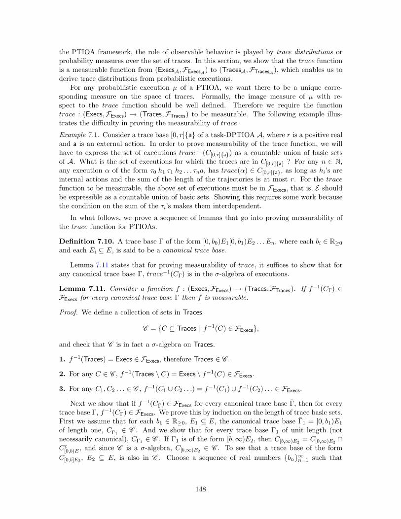
the PTIOA framework, the role of observable behavior is played by trace distributions orprobability measures over the set of traces. In this section, we show that the trace functionis a measurable function from (ExecsA,FExecsA) to (TracesA,FTracesA), which enables us toderive trace distributions from probabilistic executions.
For any probabilistic execution µ of a PTIOA, we want there to be a unique corre-sponding measure on the space of traces. Formally, the image measure of µ with re-spect to the trace function should be well defined. Therefore we require the functiontrace : (Execs,FExecs) → (Traces,FTraces) to be measurable. The following example illus-trates the difficulty in proving the measurability of trace.
Example 7.1. Consider a trace base [0, r]a of a task-DPTIOA A, where r is a positive realand a is an external action. In order to prove measurability of the trace function, we willhave to express the set of executions trace−1(C[0,r]a) as a countable union of basic setsof A. What is the set of executions for which the traces are in C[0,r]a ? For any n ∈ N,any execution α of the form τ0 h1 τ1 h2 . . . τna, has trace(α) ∈ C[0,r]a, as long as hi’s areinternal actions and the sum of the length of the trajectories is at most r. For the tracefunction to be measurable, the above set of executions must be in FExecs, that is, E shouldbe expressible as a countable union of basic sets. Showing this requires some work becausethe condition on the sum of the τi’s makes them interdependent.
In what follows, we prove a sequence of lemmas that go into proving measurability ofthe trace function for PTIOAs.
Definition 7.10. A trace base Γ of the form [0, b0)E1[0, b1)E2 . . . En, where each bi ∈ R≥0
and each Ei ⊆ E, is said to be a canonical trace base.
Lemma 7.11 states that for proving measurability of trace, it suffices to show that forany canonical trace base Γ, trace−1(CΓ) is in the σ-algebra of executions.
Lemma 7.11. Consider a function f : (Execs,FExecs) → (Traces,FTraces). If f−1(CΓ) ∈FExecs for every canonical trace base Γ then f is measurable.
Proof. We define a collection of sets in Traces
C = C ⊆ Traces | f−1(C) ∈ FExecs,
and check that C is in fact a σ-algebra on Traces.
1. f−1(Traces) = Execs ∈ FExecs, therefore Traces ∈ C .
2. For any C ∈ C , f−1(Traces \ C) = Execs \ f−1(C) ∈ FExecs.
3. For any C1, C2 . . . ∈ C , f−1(C1 ∪ C2 . . .) = f−1(C1) ∪ f−1(C2) . . . ∈ FExecs.
Next we show that if f−1(CΓ) ∈ FExecs for every canonical trace base Γ, then for everytrace base Γ, f−1(CΓ) ∈ FExecs. We prove this by induction on the length of trace basic sets.First we assume that for each b1 ∈ R≥0, E1 ⊆ E, the canonical trace base Γ1 = [0, b1)E1
of length one, CΓ1∈ C . And we show that for every trace base Γ1 of unit length (not
necessarily canonical), CΓ1 ∈ C . If Γ1 is of the form [b,∞)E2, then C[b,∞)E2= C[0,∞)E2
∩Cc[0,b)E , and since C is a σ-algebra, C[b,∞)E2
∈ C . To see that a trace base of the formC[0,b]E2
, E2 ⊆ E, is also in C . Choose a sequence of real numbers bn∞n=1 such that
148

bn+1 > bn and bn → b as n → ∞. Since for each n, C[0,bn)E1∈ C and C is a σ-algebra we
have:
C[0,b]E1=
∞⋂n=1
C[0,bn)E1∈ C .
The same holds true for basic sets of the form C(a,b)E2= C[0,b)E2
∩ C(a,∞]E2. Since every
measurable set in R≥0 is a countable union of segments of the types [0, b), (b,∞), and (a, b),we have proved that for any trace base Γ1 of unit length, CΓ1 ∈ C which implies thatf−1(CΓ1) ∈ FExecs.
In the induction step we assume that for any n ∈ N, if all canonical trace basic sets oflength n are in C , then all trace basic sets of length n are in C . Based on this inductivehypothesis and the additional assumption that every canonical trace base of length n + 1,Γ = Γn[0, bn+1)En+1 ∈ C , where Γn is a canonical base of length n, bn+1 ∈ R≥0, andEn+1 ⊆ E, we show that any trace basic set of length n + 1 is in C . The details of thisargument are similar to those in the base case.
Every set in FTraces can be expressed as a countable union of the trace basic sets, andby the hypothesis of the lemma, f−1(CΓ) is measurable for every canonical trace base Γ,and therefore f is measurable.
Our next step is to show that trace−1(CΓ) is a measurable set for every canonical tracebase Γ. In the light of lemma 7.11, this will be sufficient to conclude the measurability of thetrace function. The proof of the above statement follows from repeated application of theconstruction described by Definition 7.11. For clear exposition, we describe the constructionfor canonical trace bases of length one; the same construction is repeated for canonical basesof any finite length. The key idea is to express trace−1(C[0,r)E1
) as the countable union of adisjoint basic sets that partition [0, r) into several intervals with rational endpoints. A baseis then constructed by inserting internal actions in between the successive sub-intervals.
Definition 7.11. Let Γ1 = [0, r)E1 be a canonical trace base of unit length. For n ∈ N, ann-partition base of Γ1 is a trace base of length n of the form:
Λn,rq1,q′1,...,q
′n
∆= Q[q1, q′1]QH Q[q2, q′2]QH Q . . . [qn, q′n]QE1Q
where q1, q′1, q2, q′2, . . . , qn, q
′n ∈ Q≥0, q1 < q′1, q2 < q′2, . . . , qn < q′n, and q′1+q′2+ . . .+q′n < r.
We denote the union over all possible n-partition basic sets of Γ1 by Qn,r, that is,
Qn,r∆=
⋃q1,q′1,...,q
′n∈Q≥0
CΛn,r
q1,q′1,...,q′n,
where the union is over nonnegative rationals q1, q′1, . . . , q′n satisfying the above constraints.
In order to understand the above definitions and the proof of the following Lemma,let us consider an execution α of task-PDTIOA A, such that trace(α) ∈ CΓ1
. We knowthat α is of the form α1 a α2, where a ∈ E1 ⊆ E, α2 is any execution fragment of A,and within α1 some number (possibly 0) of internal actions occur and α1.ltime ∈ [0, r).From axiom P1 we know that the number of internal actions that occur in α1 is finite.Let us assume that this number is one. Then, α1 is of the form τ0h1τ1, where h1 ∈ Hand τ0.ltime + τ1.ltime < r. If we choose q1, q′1, q2, q
′2 ∈ Q≥0, such that τ0.ltime ∈ [q1, q′1],
149

τ1.ltime ∈ [q2, q′2], and q′1 + q′2 < r, then, α is in the basic set of Λ2,rq1,q′1,q2,q
′2. Such choices
are possible, as long as q′1 + q′2 < r, because Q≥0 is dense in R≥0,Informally, each point in the set S2 = (x0, x1) ∈ R≥0×R≥0 | x0 + x1 < r corresponds
to a possible execution fragment of the form τ0 h1 τ1, with x0 = τ0.ltime and x1 = τ1.ltime.And all such executions are included in Q2,r. To see this, notice that (a) each basic set inQ2,r, such as the C
Λ2,r
q1,q′1,q2,q′2
we chose above, covers a rectangle [q1, q′1]× [q2, q′2] ⊆ S2, and
(b) the union of all such rectangles, defined by all possible choices of q1, q′1, q2, q′2 ∈ Q≥0
satisfying q′1 + q2 < r, covers all of S2.For the general case, say, α1 = τ0 h1 τ1 . . . hn τn, with n ∈ N. Then the set Sn =
(x0, . . . , xn−1) ∈ R≥0n |∑n−1
i=0 xi < r corresponds to all possible execution fragments withn internal actions with with xi = τi.ltime, i ∈ 0, . . . , n. The union over all n-partitionsfor Γ, namely Qn,r covers all such possible executions.
Lemma 7.12. Suppose Γ1 = [0, r)E1 is a canonical trace base of a PTIOA A. Then,
trace−1(CΓ1) =
⋃n∈N
Qn,r.
Proof. First we show that⋃n∈NQn,r ⊆ trace−1(CΓ1
). Let α be an execution in Qn,r, forsome n ∈ N. Since the first n actions of α are internal actions, trace(α) is of the form τ0aα
′,where α′ is a trace of A, a ∈ E1 and τ.ltime ≤ r. By definition of trace basic set it followsthat trace(α) ∈ C[0,1)E1
.Next, we show that trace−1(CΓ1
) ⊆⋃n∈NQn,r. Consider any execution α ofA, such that
trace(α) ∈ C[0,r)E1. Then, α must be of the form α1 a α2, where a ∈ E1 and α1.ltime < r.
It suffices to show that α1 ∈ Qn,r, for some n ∈ N.By axiom P1, the number of internal actions in α′ is finite. Let us assume that the
number of internal actions in α′ is k, for some k ∈ N. We write α1 as τ0 h1 τ1 h2 . . . τk,where each hi ∈ H, and
∑ki=0 τi.ltime < r. Since the Q≥0 is dense in R≥0, there ex-
ist q0, q′0, q1, q′1, . . . , qk, q
′k ∈ Q≥0, such that, for all i ∈ 0, . . . , k, τi.ltime ∈ [qi, q′i] and∑k
i=0 q′i < r. By definition 7.11, it follows that α1 is contained in the basic set of the
k-partition base Λ = Λk,rq1,q′1,...,qk,q
′k, that is, α ∈ Qk,r.
Next we prove the generalization of Lemma 7.12 for finite length canonical trace bases.
Lemma 7.13. If Γ is a canonical trace base of A, then trace−1(CΓ) ∈ FExecs.
Proof. The proof follows from a straightforward induction on the length of the canonicaltrace base Γ. Suppose Γ = [0, r1)E1 [0, r2)E2 . . . [0, rn)En, where ri’s are nonnegative realsand Ei’s are sets of external actions, for some n ∈ N. For a canonical trace base of lengthone, by Lemma 7.12 trace−1(CΓ1
) is expressed as a countable union of bases, and thereforeis a measurable set.
Suppose the lemma holds for all canonical trace basic sets of length n, for some n ∈ N.Consider a canonical trace base Γ = Γn[0, r) E1 of length n+ 1, where Γn+1 is a canonicaltrace base of length n, r ∈ R≥0, and E1 ⊆ E. From the induction hypothesis we know thattrace−1(CΓn
) = ∪i∈IC∆i , for some countable collection of basic sets indexed by I. Herethe ∆i’s are concatenation of partition bases for the sets in Γn. We extend the ∆i’s with ak-partition base Λk,r for the trace base [0, r)E1. Then, using essentially the same arguments
150

as in Lemma 7.12 it can be shown that:
trace−1(CΓ) =⋃i∈I
⋃k∈N
C∆iΛk,r (2k rational parameters of Λk,r are suppressed.)
=⋃i∈I
⋃k∈N
⋃q1,q′1,...,qk,q
′k∈Q≥0
C∆iΛ
k,r
q1,q′1,...,qk,q′k
.
Here the union over q1, q′1, . . . , qk, q′k ∈ Q≥0 is taken for those rationals that satisfy the usual
restrictions, that is, q1 < q′1, . . . , qk < q′k, and∑q′i < r. Since trace−1(CΓ) is a countable
union of basic sets it is contained in the σ-algebra FExecs.
Theorem 7.14. trace : (Execs,FExecs) → (Traces,FTraces) is a measurable function.
Proof. It follows from Lemmas 7.13 and 7.11 that for any trace base Γ, trace−1(Γ) is acountable union of disjoint basic sets. This suffices to establish measurability of the tracefunction.
Theorem 7.14 implies that corresponding to each probabilistic execution µ of a given task-DPTIOA A there exists a unique probability measure on the set of traces of A, namely, theimage measure of µ under the trace function. This probability measure on TracesA is calledthe trace distribution corresponding to µ. From Section 7.4.2 we saw that each task scheduleρ of a task-DPTIOA gives rise to a probabilistic execution µρ. Thus, each task schedule alsogives a corresponding trace distribution which we denote by tdist(µρ), or in short as tdist(ρ).More formally, tdist(ρ) : TracesA → [0, 1], is defined as tdist(ρ)(E) = µρ(trace−1(E)), forany measurable set E ∈ FTracesA . The set of trace distributions of A, TdistsA, is the set oftdist(ρ)’s for any task schedule ρ of A.
7.5 Implementation and Compositionality
In the previous section we defined the set of trace distributions of a task-DPTIOA A. Anatural definition for implementation of task-DPTIOAs would be to say A1 implementsA2, if and only if TdistsA1 ⊆ TdistsA2 . This definition, however, does not give the desirablesubstitutivity property of the type stated by Theorem 2.5, for example. Instead, based onthe idea presented in [CCK+06a], we define a notion of external behavior and show that theimplementation relation based on this external behavior is compositional. We formulatethe external behavior of a A as a mapping from possible “environments” for A to sets oftrace distributions that can arise when A is composed with the given environment.
Definition 7.12. An environment for task-DPTIOA A is a PTIOA E such that A and E arecompatible and their composition A||E is closed. The external behavior of a task-DPTIOAA, written as ExtBehA, is defined as a function that maps each environment PTIOA E forA to the set of trace distributions TdistsA||E .
Definition 7.13. Two task-DPTIOAs A1 and A2 are comparable if E1 = E2. If A1 andA2 are comparable then A1 is said to implement A2, written as A1 ≤ A2 if, for everyenvironment PTIOA E for both A1 and A2, ExtBehA1(E) ⊆ ExtBehA2(E).
151

This definition of implementation as a functional map from environment automata givesus the desired compositionality result for task-DPTIOAs.
Theorem 7.15. Suppose A1, A2 and B are task-DPTIOAs, where A1 and A2 are compa-rable and A1 ≤ A2. If B is compatible with A1 and A2 then A1||B ≤ A2||B.
Proof. Let E be an environment task-DPTIOA for both A1||B and A2||B. Consider atask schedule ρ1 for the composed task-DPTIOA (A1||B)||E . Let η = tdist(ρ1) be thetrace distribution of (A1||B)||E generated by ρ1. It suffices to show that η is also a tracedistribution of (A2||B)||E , generated by some task schedule.
As ρ1 is a task schedule for A1||(B||E) it generates the same trace distribution η forPTIOA A composed with the environment B||E . Further B||E is also a closing environmentfor A2 because A1 and A2 are compatible. As A1 ≤ A2, there exists a task schedule ρ2 forA2||(B||E) that generates the trace distribution η. It follows that ρ2 is a task schedule for(A2||B)||E that produces the trace distribution η.
7.6 PTIOAs and Local Schedulers
In this section, we develop the probabilistic semantics for PTIOAs that do not necessarilysatisfy the determinism axioms D1, D2, and D3. This development relies on local schedulerswhich are task-DPTIOAs.
Definition 7.14. A Generalized PTIOA A = (X, (Q,FQ), x, A,D, T ,R), where all thecomponents except T and R are defined as in Definition 7.1.
(a) T is a set of trajectories for Q that is closed under prefix, suffix, and concatenation.Further, for any x ∈ Q,℘(x) ∈ T .
(b) R is an equivalence relation on the local actions. The equivalence classes of R are calledtasks.
Indeed, a generalized PTIOA A is similar to a task-PTIOA except that its trajectoriesare not necessarily deterministic and it may not necessarily satisfy D1, D2, and D3. Stateof a A may change through nondeterministic choice of actions and also through choice ofdistinct, non-point trajectories starting.
Definition 7.15. A local scheduler for generalized PTIOA A = (X, (Q,FQ), x, A,D, T ,R),is a task-DPTIOA S = (XA, (QA,FQA), xA, AA,D′, T ′,RA) that is identical to A exceptthat D′ ⊆ DA and T ′ ⊆ TA, such that T ′ is deterministic and S satisfies D1-3.
A probabilistic system captures the notion of possible ways of resolving internal nonde-terminism in a generalized PTIOA. Formally, a probabilistic-system is a pair M = (A,L ),where A is a generalized PTIOA and L is a set of local schedulers for A. The notions ofprobabilistic execution and trace distribution defined earlier for task-DPTIOAs, carry overnaturally to generalized PTIOAs. A probabilistic execution for M is defined to be anyprobabilistic execution of S, for any S ∈ L .
Compatibility and composition of generalized PTIOAs is defined in the same way as inthe case of task-DPTIOAs (see, Definition 7.4). We remind the reader that the compositionA = A1||A2 of compatible generalized PTIOAs A1 and A2, is also a generalized PTIOAonly if A satisfies M2. In order to avoid restating this condition in all our definitions and
152
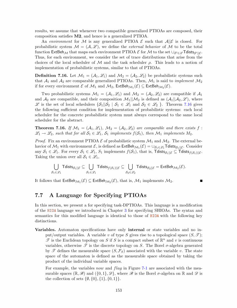
results, we assume that whenever two compatible generalized PTIOAs are composed, theircomposition satisfies M2, and hence is a generalized PTIOA.
An environment for M is any generalized PTIOA E such that A||E is closed. Forprobabilistic system M = (A,L ), we define the external behavior of M to be the totalfunction ExtBehM that maps each environment PTIOA E for M to the set ∪S′∈L TdistsS′||E .Thus, for each environment, we consider the set of trace distributions that arise from thechoices of the local scheduler of M and the task scheduler ρ. This leads to a notion ofimplementation of probabilistic systems, similar to that of PTIOAs.
Definition 7.16. Let M1 = (A1,L1) and M2 = (A2,L2) be probabilistic systems suchthat A1 and A2 are comparable generalized PTIOAs. Then, M1 is said to implement M2
if for every environment E of M1 and M2, ExtBehM1(E) ⊆ ExtBehM2(E).
Two probabilistic systems M1 = (A1,L1) and M2 = (A2,L2) are compatible if A1
and A2 are compatible, and their composition M1||M2 is defined as (A1||A2,L ), whereL is the set of local schedulers S1||S2 | S1 ∈ L1 and S2 ∈ L2 . Theorem 7.16 givesthe following sufficient condition for implementation of probabilistic systems: each localscheduler for the concrete probabilistic system must always correspond to the same localscheduler for the abstract.
Theorem 7.16. If M1 = (A1,L1), M2 = (A2,L2) are comparable and there exists f :L1 → L2, such that for all S1 ∈ L1, S1 implements f(S1), then M1 implements M2.
Proof. Fix an environment PTIOA E of probabilistic system M1 and M2. The external be-havior of M1 with environment E , is defined as ExtBehM1(E) = ∪S1∈L1TdistsS1||E . Considerany S1 ∈ L1. For every S1 ∈ L1, S1 implements f(S1), that is, TdistsS1||E ⊆ Tdistsf(S1)||E .Taking the union over all S1 ∈ L1,⋃
S1∈L1
TdistsS1||E ⊆⋃
S1∈L1
Tdistsf(S1)||E ⊆⋃
S2∈L2
TdistsS2||E = ExtBehM2(E).
It follows that ExtBehM1(E) ⊆ ExtBehM2(E), that is, M1 implements M2.
7.7 A Language for Specifying PTIOAs
In this section, we present a for specifying task-DPTIOAs. This language is a modificationof the HIOA language we introduced in Chapter 3 for specifying SHIOAs. The syntax andsemantics for this modified language is identical to those of HIOA with the following keydistinctions.
Variables. Automaton specifications have only internal or state variables and no in-put/output variables. A variable v of type S gives rise to a topological space (S,T );T is the Euclidean topology on S if S is a compact subset of Rn and v is continuousvariables, otherwise T is the discrete topology on S. The Borel σ-algebra generatedby T defines the measurable space (S,FS) associated with the variable v. The statespace of the automaton is defined as the measurable space obtained by taking theproduct of the individual variable spaces.
For example, the variables now and flag in Figure 7-1 are associated with the mea-surable spaces (R,B) and (0, 1,D, where B is the Borel σ-algebra on R and D isthe collection of sets ∅, 0, 1, 0, 1.
153
Initial state. Each state variable is initialized to a single value. These initial valuationstogether define the unique starting state of the automaton.
Transitions. The precondition-effect style of HIOA is used to define the transitions. How-ever, the effects of transitions are either purely deterministic or probabilistic. Thatis, nondeterministic choose statements are not allowed. Probabilistic transitions aredefined by a new type of choose statement that specifies the distribution accordingto which this choice is made.
For example, the statement xs := choose Normal(x, σ) of in Figure 7-1 means thatxs is chosen according to a normal probability distribution with mean x and standarddeviation σ. The statement toss := choose 1, 0 Disc[12 ,
12 ] means that toss is
assigned a value 0 or 1 with probability 12 each.
Trajectories. State models are used to specify the set of trajectories of a PTIOA. Anadditional requirement is that the set of trajectories should be deterministic, i.e., thestate models should have differential equations with unique solutions.
The state model normal of Example 7.2 specifies that along any trajectory the contin-uous variable now increases at the same rate as that of real time, until the stoppingcondition is satisfied. Hence, normal specifies a deterministic set of trajectories.
Tasks. A new language construct is introduced to HIOA for specifying the set of tasks ofthe PTIOA. The tasks section of the code specifies the tasks as a sequence of sets ofactions. In the PTIOA of Example 7.2, sample and send actions constitute the oneand only task.
In the remaining part of this section we use this language for specifying two typicaltask-PTIOAs and then, we illustrate some of the concepts we defined earlier in the contextof these examples.
Example 7.2. The automaton NoisySensor(d, σ) of Figure 7-1 specifies a sensor that pe-riodically reports the sampled value xs of a variable x that is evolving according to thedifferential equation d(x) = f(x). The value is reported through the occurrence of thesend(xs) action which immediately follows the sample action. The sample action occursperiodically, every d time units, and assigns a value to xs. The state variables, actions,transitions, and trajectories are specified in the same way as in HIOA specifications with thefollowing differences. It is routine to check that NoisySensor satisfies the axioms of Defini-tion 7.2. This automaton has several similarities with the Sensor automaton of Figure 4-4.Here, the sampled value xs is chosen according to a normal probability distribution withmean x and standard deviation σ whereas in Sensor, the choice of the sampled value x0
was made nondeterministically over the interval [θ0s − e0, θ
0s + e0]. In many applications,
such as sensors, probabilistic information about uncertainties is available, and in those casesPTIOA models can capture this extra information.
Example 7.3. The Ben-Or consensus protocol [BO83] is a randomized algorithm for n fault-prone processors to agree on a valid value by communicating over an asynchronous network.The algorithm proceeds in a sequence of stages. In each stage, nonfaulty processes sendand receive messages based on coin-flips and comparison of values. With perfectly unbi-ased coins, a stage ends successfully with probability 1
2n , and all nonfaulty processes agreeon a value. After one communication round of a successful stage the consensus value isdisseminated. An unsuccessful stage is followed by the beginning of the next stage.
154

automaton NoisySensor(d, σ : Real)signature
internal sampleoutput send(xs : Real)
variablesinternal now : Real := 0;next sample : AugmentedReal := 0;x : Real := 0;xs : Real := 0;flag : Bool := f alse;
transitionsinternal sample
pre now = next send;eff xs := choose Normal(x, σ);flag := true; next send := now + d;
output send(m)pre flag ∧ (xs = m);eff flag := f alse;
trajectoriestrajdef normal
stop when now = next send ∨ flag;evolve d(x) = f(x);
taskssend, sample
Figure 7-1: Noisy sensor.
The Consensus PTIOA of Figure 7-2 abstracts the actual computation performed bythe processes as well as the messages exchanged, and specifies the termination behavior ofthe Ben-Or protocol in a terms of number of stages and time elapsed. The stage variablerepresents the current stage of the protocol. The phase variable is 0 at the beginning ofa stage, 1 when a stage completes successfully, and 2 when the protocol terminates at allnonfaulty processes.
The try action models the computation and communication within a stage. With prob-ability 1 − 1
2n it leads to the next stage and with probability 12n it leads to phase 1 of the
current stage. This is specified by the probabilistic choose statement which assigns tophase the value 1 with probability 1
2n and 0 with probability 1 − 12n . The decide action
marks the termination of the protocol.The trajectories section specifies that along any trajectory, timer increases at the
same rate as real time, and that all other variables remain constant. The amount of timethat elapses in phase 0 owing to message delays is modeled by an exponential distributionwith parameter λ0. Specifically, the delay variable is assigned a value chosen from thisdistribution and stop when condition together with the pre condition of try forces theaction to occur when timer equals delay. Likewise, the amount of time that elapses inphase 1 is modeled by an exponential distribution with parameter λ1. The tasks sectionof the code specifies the two tasks of the automaton.
A typical execution of the Consensus automaton is a sequence
α = τ0 try τ1 try τ2 decide τ3,
were each τi, i ∈ 0, . . . , 3, is a trajectory over which timer increases monotonically at thesame rate as real time and all other variables remain constant. The length of the trajectoryτi, i ∈ 0, 1, 2 in each stage is determined by the value of the variable delay, which ischosen according to the exponential distribution with parameter λ0. The correspondingtrace is:
trace(α) = (τ0 _ τ1_ τ2 ↓ ∅) decide (τ3 ↓ ∅).
Notice that the trace contains information about the total time elapsed before decide occursbut not the amount of time that is spent in individual stages.
Let us examine how Definition 8.3 assigns probability measures to the basic sets of the
155

Consensus(n : Nat, λ0, λ1, p : Real)where λ0, λ1 > 0, 0 < p < 1
signatureinternal tryoutput decide
variablesinternal stage : Nat := 1; phase : 0, 1, 2 := 0;timer : Real := 0;delay : AugmentedReal := t0;
transitionsoutput decide
pre timer = delay ∧ phase = 1;eff timer := 0; phase:= 2; delay:= ∞;
output trypre timer = delay ∧ phase = 0;eff timer := 0;
phase:= choose 1,0 Disc 12n , 1− 1
2n ;if phase = 0
then stage:= stage+ 1; delay:= choose Exp(λ0);else delay:= choose Exp(λ1) fi
trajectoriestrajdef normal
stop when timer = delay;evolve d(timer) = 1;
taskstrydecide
Figure 7-2: Randomized consensus with exponential message delays.
Consensus automaton. Recall that a state x of Consensus is an ordered 4-tuple specifyingthe valuations of the 4 variables stage, phase, timer, and delay, respectively. From thespecification in Figure 7-2, x = (1, 0, 0, t0) and we define x′ = (1, 0, t0, t0). Suppose µ1 =apply(δx, λ), where λ is the empty task schedule, Let Λ1 = Q0R0Q1, such that x ∈ Q0 ∈ FQ,x′ ∈ Q1 ∈ FQ, and t0 ∈ R0. Then, by Definition 8.3, µ1(CQ0) = 1 and µ1(CΛ1) = 1. Infact, for any base Λ′1 = Q0 R
′0 Q
′1, µ1(CΛ′1
) = 1, if there exists t < t0, such that t ∈ R′0 and(1, 0, t, t0) ∈ Q′1. For any base Λ1 A1 Q2 of Λ1 R2 Q
′2 that extends Λ1, the measure assigned
is 0.Next, suppose µ2 = apply(µ1, try). Let Λ2 = Λ1 tryQ2, Q2 = x | x d stage = 2,x d
phase = 0,x d delay ≤ r1, for some r1 ∈ R≥0. Then,
µ2(CΛ2) =∫s∈G
µs(Q2)µ1(dα), where G = x | gΛ1,try(x),
=(
1− 12n
)(1− eλ0r1).
Since µ1(α) = 1 for a single execution which is a trajectory starting from x and ending at x′,in the above case the integral of Equation (7.3) reduces to µx′(Q2). Suppose Λ3 = Λ2R1Q3
where R1 = [0, r′1], where r′1 ≤ r1, and Q3 = x | x d stage = 2,x d phase = 0,x dtimer ≤ x d delay ≤ r1. Then Equation (7.4) gives: µ2(CΛ3) = r′1
r112n (1 − eλ0r1). Suppose
Q′2 = x | x d stage = 0,x d phase = 1,x d delay ≤ r2, Λ′2 = Λ1 tryQ′2, then
µ2(CΛ′2) =
∫s∈G
µs(Q2)µ1(dα), where G = x | gΛ1,try(x),
=12n
(1− eλ0r2).
Taking another step, suppose µ3 = apply(µ2, decide). Let Q4 = x | x d stage = 0,x dphase = 2,x d delay ≤ r2, where r2 ∈ R≥0. From Equation (7.3) we obtain:
µ3(CΛ′2decideQ4) =
12n
(1− eλ0r1)(1− eλ1r2),
µ3(CΛ2) = µ2(CΛ2) =(
1− 12n
)(1− eλ0r1).
156

The distributions µ1, µ2, and µ3 are the probabilistic executions of Consensus correspondingto the task schedules λ, try, and trydecide.
7.8 Summary
We have introduced PTIOAs for modelling and discretely communicating probabilistic hy-brid systems. The non-probabilistic aspects of the behavior of a PTIOA, namely, its exe-cutions and its traces are defined in the same way as in the case of SHIOAs. In order toassociate probability measures with sets of executions of a PTIOA, first, we had to ensuremeasurability of all reasonable sets of executions. For this purpose, we found it natural towork with a measurable state space Q, that is, Q associated with the additional structureof a σ-algebra FQ. Introducing two new measurability axioms, namely, M1 and M2 weconstructed the σ-algebra FExecsA over the space of executions of task-DPTIOA A. Weshowed that a PTIOA A combined with a local scheduler (for resolving internal nonde-terminism), and an oblivious task scheduler (for resolving external nondeterminism) givesrise to a probabilistic execution—a probability distribution over the measurable space ofexecutions (ExecsA,FExecsA). The probabilistic behavior of PTIOAs is defined in termsof sets of probabilistic executions—one for each possible local and task schedule. Basedon probabilistic execution we define trace distributions and implementation relations forPTIOAs.
We show that the composition of two PTIOAs is also a PTIOA only if the composite au-tomaton satisfies an additional measurability requirement, namely, axiom M2. This couldbe improved by imposing restrictions on the trajectories or with additional measurabilityrequirements, so that a subclass of PTIOAs is closed under composition. In the futurewe will extend PTIOAs to support external variables. For including input variables onehas to remove the the time-action determinism axiom D3 because the stopping points of atrajectory would also depend on inputs. We also intend to develop a suite of verificationtechniques for quantitative properties such as, probabilistic safety and stochastic stabil-ity [CL06]. In Chapter 8 we present techniques for verifying approximate implementationrelations for a class of “discrete” PTIOAs. Such techniques are particularly relevant incontext of PTIOAs because inaccuracies related to timing information can be captured byapproximate abstractions. A longer term research direction is to incorporate continuousstochastic behavior over trajectories.
157
Chapter 8
Verifying ApproximateImplementation Relations
In this chapter we introduce the notion of approximate implementation for ProbabilisticI/O Automata (PIOA) and develop methods for proving such relationships. A PIOA isessentially a “discrete” pre-PTIOA (of Chapter 7); it does not have trajectories and onlydiscrete probability distributions appear in transition definitions. The nondeterminism ina PIOA is resolved by task schedulers which gives rise to probabilistic executions and tracedistributions. A PIOA A is said to implement PIOA B, in the traditional sense, if eachtrace distribution of A is also a trace distribution of B. But small perturbations to theparameters of A produces traces distributions with slightly different probabilities and thisbreaks the implementation relation. We would like to define and verify implementationrelations that not only capture the binary fact of whether or not A implements B, but alsothe degree to which A implements B. To this end, we develop new notions of approximateimplementation for PIOAs and generalizing existing simulation relations propose real-valuedsimulation functions for proving approximate implementations.
In Section 8.2.2 we briefly describe the semantics of PIOAs. We relax the notion ofimplementation by taking into consideration the “similarity” of trace distributions that arenot exactly equal. In Sections 8.3 and 8.4 we introduce two different metrics for measuringsimilarity of trace distributions; each of these give rise to corresponding notions of approx-imate implementation and we develop simulation-based techniques for verifying them. InSections 8.3.5 and 8.4.3, we discuss applications of approximate implementations to verifi-cation of probabilistic safety and termination.
8.1 An Overview
Implementation relations play a fundamental role in the study of complex interacting sys-tems because they allow us to prove that a given concrete system implements an abstractspecification. An automaton A is said to implement another automaton B if the observablebehavior of the first is subsumed by that of the latter. In the non-probabilistic setting,we saw applications of implementation relations in verifying safety (Chapter 4) and sta-bility (Chapter 5). These notions of implementation rely on equality of observable behav-ior. That is, every observable behavior of the concrete system must be exactly equal tosome observable behavior of the abstract specification. It has been well-known for sometime now that such strict equality based implementation relations are not robust (see,
158

e.g., [JS90, DJGP02, GJP04]). Small perturbations to the parameters of the system pro-duces traces with slightly different numbers (representing say, timing or probability infor-mation), and thus breaks the equality between traces. One way to overcome this problem isto relax the notion of implementation by taking into consideration the “similarity” of tracesusing a metric. Apart from providing robust implementation relations, notions of approx-imate implementation also enable us to create abstract models without introducing extranondeterminism. For instance, a complex trajectory τ of a hybrid system can be abstractedby a simpler set of trajectories which envelop τ . Such an abstraction achieves simplicity,and perhaps tractability, but sacrifices determinism. On the other hand, τ could be ap-proximately abstracted by a single simpler trajectory τ ′, but now, the abstract model is notimplemented by the concrete model, at least not in the traditional sense. We can, however,quantify the closeness of the abstract and the concrete systems using some appropriatenotion of approximate implementation based some metric over trajectories.
Probabilistic I/O Automata (PIOA) were introduced by Segala in [Seg95b, Seg95a]for the purpose of modeling and verifying untimed, randomized, distributed algorithms.Task-structured PIOAs (task-PIOAs) [CCK+06c, CCK+06a] introduce an additional taskstructure to PIOAs which makes it possible to resolve nondeterminism by a simple sequenceof tasks. In this chapter we introduce the notion of approximate implementations for task-PIOAs. Parts of this work previously appeared in [ML06] and [ML07]. A task-PIOA isa nondeterministic automaton with a countable state space. A task-PIOA interacts witha task scheduler to give rise to a trace distribution—a probability distributions over itstraces. A task-PIOA is said to (exactly) implement another task-PIOA if the set of tracedistributions of the first is a subset of the trace distributions of the latter. Implemen-tations, simulation relations for proving implementations, and compositionality results fortask-PIOAs are presented in [CCK+06b]. A special kind of approximate implementation re-lation that tolerates small differences in the probability of occurrence of a particular actionis used in [CCK+06d] to verify a security protocol. In contrast, the notions of approxi-mation introduced here can be used to quantify discrepancies in the distributions of any(measurable) function, that is, any random variable on the space of trace distributions.
In Section 8.3 we define uniform approximate implementations for task-PIOAs based onthe uniform metric on trace distributions. A PIOA A is a δ-approximate implementation ofanother PIOA B, for a positive δ, if the for any trace distribution of A, there exists a tracedistribution of B such that their discrepancy, with respect to the uniform metric, over anymeasurable set of traces is at most δ. We present Expanded Approximate Simulations (EAS)for proving uniform approximate implementations. EAS is a natural generalization of thesimulation relation presented in [CCK+06d]. Let µ1 and µ2 be probability distributionsover executions of task-PIOAs A and B. An EAS from A to B is a function φ mappingeach µ1, µ2 pair to a nonnegative real. The number φ(µ1, µ2), is a measure of how similarµ1 and µ2 are in terms of producing similar trace distributions. Informally, if φ(µ1, µ2) ≤ ε,for some ε ≥ 0, then it is possible to closely (with respect to the uniform metric on tracedistributions) simulate from µ2 anything that can happen from µ1, and further, the resultingdistributions, say µ′1 and µ′2, are also close in the following sense. There exists a jointdistribution ψ supported on the set (η1, η2) | φ(η1, η2) ≤ ε such that the first and thesecond marginal distributions of ψ have means µ′1 and µ′2. Informally, this means that µ′1and µ′2 can be decomposed into a set of measures that are close in the sense of φ.
In Section 8.4, we define discounted uniform approximate implementations of task-PIOAs based on the discounted uniform metric on trace distributions, respectively. Uniformapproximate implementations are useful for deducing probabilistic safety properties. How-
159

ever, since they gives absolute bounds on the discrepancy over any set of traces, they do notgive us useful information when the probability of the set itself is smaller than the approxi-mation factor δ. In order to obtain useful bounds on the discrepancies over a sequence of setsof traces that have monotonically decreasing probabilities, the notion of discounted uniformapproximate implementation is useful. PIOA A to be a δk-discounted approximate imple-mentation of B, if the for any trace distribution of A, there exists a trace distribution of Bsuch that their discrepancy over any trace of length k is at most δk; here δkk∈N is a collec-tion of discount factors. We define Discounted Approximate Simulations (DAS) in a similarway as we defined EAS and prove that they are sound for proving discounted approximateimplementations. We demonstrate the utility of discounted approximate implementationsand DASs by proving that the probability of termination of an ideal randomized consensusprotocol (after a certain number of rounds) is close to the same probability for a protocolthat uses biased coins.
Throughout the chapter we assume that the task-PIOAs in question are closed and inSection 8.5 we outline how our results extend to general (not necessarily closed) task-PIOAs.We start the chapter by giving the basic definitions and results for task-PIOAs; we referthe reader to [CCK+05] for a detailed treatment.
8.2 Task-structured PIOA
In this section we present the basic definitions and results for task-PIOAs. The notations forsets, functions, and variables from Section 2.1 of Part I and those for σ-algebras, measurablespaces, and measures from Section 7.2, have the same meanings in this chapter. Given a setQ, we denote a σ-algebra over Q by FQ, the set of discrete (sub-) probability measures onX by Disc(Q) (resp. SubDisc(Q)). If µ is a discrete probability or sub-probability measureon X, the support of µ, written as supp(µ), is the set of elements of X that have non-zeromeasure.
8.2.1 Definition of Task Structured PIOA
The task-PIOA model used in this chapter is slightly more general than the one in [CCK+06b]because we allow the starting configuration of an automaton to be any distribution overstates and not just a Dirac mass.
Definition 8.1. A task-structured Probabilistic I/O Automaton (task PIOA) A = (X, Q, ν,A, D, R), where:
(a) X is a set of internal or state variables,
(b) Q ⊆ val(X) is a countable set of states, ν ∈ Disc(Q) is the starting distribution onstates;
(c) A is a countable set of actions, partitioned into internal H, input I, and output Oactions. L = O ∪ H is the set of local actions and E = O ∪ I is the set of externalactions. The set of external actions of A is E := I ∪O and the set of locally controlledactions is L := O ∪H.
(d) D ⊆ Q× A× Disc(Q) is set of discrete transitions. An action a is enabled in a statex if (x, a, µ) ∈ D for some µ. In this case, we write x a→ µ.
160

(e) R is an equivalence relation on the locally controlled actions. The equivalence classesof R are called tasks. A task T is enabled in a state x if some action a ∈ T is enabledin x.
In addition, A satisfies:
E1 (Input enabling) For every x ∈ Q and a ∈ I, x ∈ Ea.D1 (Transition determinism) For every x ∈ Q and a ∈ A, there is at most one
µ ∈ Disc(Q) such that (x, a, µ) ∈ D.
D2 (Action determinism) For every x ∈ Q and T ∈ R, at most one a ∈ T isenabled in x.
Notations. A task PIOA is closed if its set of input actions is empty. We denote thecomponents of a task PIOA A by XA, QA, xA,DA etc., and the components of a task PIOAAi by Xi, Qi,xi,Di, etc.
The input enabling axiom E1 is identical to the standard non-blocking axiom for non-probabilistic and probabilistic hybrid system models (see, Definitions 2.7 and 7.1. Of course,the other non-blocking axiom, namely, E2 input trajectory enabling, is not relevant forPIOAs. Also, the measurability axioms, such as M1 and M2 of PTIOAs, are unnecessarybecause: (a) the state space Q is countable and it is equipped with the σ-algebra generatedby the discrete topology on Q. That is, every subset of Q is measurable. And (b) thetransitions give rise to discrete probability distributions. Axioms D1 and D2 are the sameas in the case of task-DPTIOAs (see, Definition 7.2). These axioms together with the taskstructure on local actions enable us to systematically resolve the nondeterminism in a PIOA.
8.2.2 Executions and Traces
An execution fragment of A is a finite or infinite sequence α = q0 a1 q1 a2 . . . of alternatingstates and actions, such that (i) if α is finite, then it ends with a state; and (ii) for everynon-final i, there is a transition (qi, ai+1, µ) ∈ D with qi+1 ∈ supp(µ). We write α.fstatefor q0, and, if α is finite, we write α.lstate for its last state. We use FragsA (resp., Frags∗A)to denote the set of all (resp., all finite) execution fragments of A. An execution of A is anexecution fragment beginning from some state in supp(ν). ExecsA (resp., Execs∗A) denotesthe set of all (resp., finite) executions of A. The trace of an execution fragment α, writtentrace(α), is the restriction of α to the set of external actions of A. We say that β is a traceof A if there is an execution α of A with trace(α) = β. TracesA (resp., Traces∗A) denotesthe set of all (resp., finite) traces of A.
8.2.3 Composition of Task-PIOAs
The composition operation on task-PIOAs enable us to construct a PIOAs representing acomplex system from two interacting PIOAs by identifying their external actions. PIOAs donot have external (input/output) variables and component automata communicate throughexternal actions only.
Composition of a pair of PIOAs is defined as follows:
Definition 8.2. Task-PIOA A1 and A2 are compatible if X1 ∩X2 = H1 ∩A2 = H2 ∩A1 =O1 ∩ O2 = ∅. If A1 and A2 are compatible task-PIOAs then their composition A1||A2 isdefined to be A = (X,Q, ν, A,D,R), where:
161

(a) X = X1 ∪X2,
(b) Q = Q1 ×Q2, and the initial distribution ν is defined as ν(x1,x2)∆= ν1(x1) × ν2(x),
for xi ∈ Qi, i ∈ 1, 2.
(c) A = A1 ∪A2, I = (I1 ∪ I2) \ (O1 ∪O2), O = O1 ∪O2, H1 ∪H2,
(d) D ⊆ Q×A×Disc(Q) is the set of triples ((x1,x2), a, µ1×µ2) such that for i ∈ 1, 2,if a ∈ Ai then (qi, a, µi) ∈ Di, otherwise µi = δxi ,
(e) R = R1 ∪R2.
It can be checked easily that the composite structure A is also a task-PIOA.
8.2.4 Probabilistic Executions and Trace Distributions
So far we have presented the concepts concerning non-probabilistic behavior of PIOAs. Inthis section, we present definitions and results from [CCK+06a] which describe the proba-bilistic semantics of PIOAs.
For any finite execution fragment α of A, the cone of α, denoted by Cα, is the set of exe-cution fragments that have α as prefix. The σ-algebra generated by cones of finite executionfragments of A is denoted by FExecsA . This defines a measurable space (ExecsA,FExecsA)in which any set of finite execution fragments is measurable. A probability measure on(ExecsA,FExecsA) is called a probabilistic execution.
Nondeterministic choices in A are resolved using a task scheduler—an entity whichchooses a task—which in turn probabilistically determines the next state of the automaton.One could define various kinds task schedulers by specifying what dynamic informationmay be used in choosing the next task. We refer the reader to Section 7.4.2 for a discussionon the different kinds of schedulers. The probabilistic semantics of task-PIOAs with ageneral class of history dependent schedulers has been developed in [CCK+06b]. In thischapter, we restrict our attention to oblivious schedulers that do not depend on dynamicinformation generated during execution. A task schedule for A is any finite or infinitesequence ρ = T1T2 . . . of tasks in R. Although restrictive this class of schedulers arisenaturally in many applications, including in analysis of security protocols [CCK+06c]. Ascheduler ρ and a finite execution fragment α generate a measure µρ,α on (ExecsA,FExecsA).
A task schedule generates a probabilistic execution of the task-PIOA A by repeatedlyscheduling tasks, each of which determines at most one transition of A. Formally, we definean operation that “applies” a task schedule to a task-PIOA:
Definition 8.3. Let A be an action-deterministic task-PIOA. Given µ ∈ Disc(Frags∗A) anda task schedule ρ, apply(µ, ρ) is the probability measure on FragsA defined recursively by:
1. apply(µ, λ) ∆= µ, where λ denotes the empty sequence of tasks.
2. apply(µ, T ) ∆= p1 + p2, where T is a task and p1, p2 are defined as follows: For every
162

α ∈ Frags∗A:
p1(α) ∆=
µ(α′)η(q) if α = α′ a q, such that a ∈ T and α′.lstate a→ η,
0 otherwise.
p2(α) ∆=
µ(α) if T is not enabled in α.lstate,
0 otherwise.
3. apply(µ, ρ) ∆= apply(apply(µ, ρ′), T ), where ρ = ρ′ T , T ∈ R.
4. apply(µ, ρ) ∆= limi→∞(µi), where ρ is infinite ρi is the length-i prefix of ρ, and µi =apply(µ, ρi).
In Case (2) above, p1 represents the probability that α is executed when applying task Tat the end of α′. Because of transition-determinism and action-determinism, the transitionα′.lstate
a→ η is unique, and so p1 is well-defined. The term p2 represents the originalprobability µ(α), which is relevant if T is not enabled after α. It is routine to check thatthe limit in Case (4) is well-defined. The other two cases are straightforward. Given anytask schedule ρ, apply(ν, ρ) is a probability distribution over ExecA. Several useful propertiesof the apply(, ) function relating sequences of probability distributions on executions andtraces are given in Appendix 8.8.
The lstate function is a measurable function from the discrete σ-algebra on finite exe-cution fragments of A to the discrete σ-algebra of states of A. If µ is a probability measureon execution fragments of A, then we define the lstate distribution of µ, lstate(µ), to bethe image measure of µ under the lstate function.
We note that the trace function is a measurable function from FExecsA to the σ-algebragenerated by cones of traces. Thus, given a probability measure µ on FExecsA we definethe trace distribution of µ, denoted tdist(µ), to be the image measure of µ under the tracefunction. We extend the tdist() notation to arbitrary measures on execution fragments ofA. We write tdist(µ, ρ) as shorthand for tdist(apply(µ, ρ)), the trace distribution obtainedby applying task schedule ρ starting from the measure µ on execution fragments. We writetdist(ρ) for tdist(apply(ν, ρ)). A trace distribution of A is any tdist(ρ). We use TdistsA todenote the set tdist(ρ) : ρ is a task schedule forA of all trace distributions of A.
8.2.5 Exact implementations and Simulations
Two task-PIOAs A1 and A2 are comparable if they have the same set of external actions.The implementation relation for comparable task-PIOAs is defined in terms of inclusion ofsets of trace distributions.
Definition 8.4. Given comparable closed task-PIOAs A1 and A2, A1 is said to implementA2 if TdistsA1 ⊆ TdistsA2 . If A1 and A2 implement each other then they are said to beequivalent .
In [CCK+06b] a simulation relation for closed, task-PIOAs is defined and it is shownto be sound for proving the above implementation relation. This definition is based onthree operations involving probability measures: flattening, lifting, and expansion. First wedefine these operations.
163

The flattening operation takes a discrete probability measure over probability mea-sures and “flattens” it into a single probability measure. Let Q and P be a sets. Ifη ∈ Disc(Disc(Q)), then the flattening of η, denoted by flatten(η) ∈ Disc(Q), is definedby flatten(η) =
∑µ∈Disc(Q) η(µ)µ.
The lifting operation takes a relation R⊆ Q × P and “lifts” it to a relation L(R)⊆Disc(Q) × Disc(P ) Informally, a measure µ1 on Q is related to a measure µ2 on P if µ2
can be obtained by redistributing the probabilities assigned by µ1, in such a way that therelation R is respected. The lifting of R, denoted by L(R), is a relation from Disc(Q) toDisc(P ) defined by: µ1 L(R) µ2 iff there exists a weighting function w : Q × P → R≥0
such that: (i) for each q ∈ Q and p ∈ P , w(q, p) > 0 implies q R p, (ii) for each q ∈ X,∑y w(q, p) = µ1(q), and (iii) for each p ∈ Y ,
∑pw(q, p) = µ2(p).
Finally, the expansion operation takes a R⊆ Disc(P ) × Disc(Q), and returns a relationE(R)⊆ Disc(Q) × Disc(P ) such that µ1 E(R) µ2 whenever they can be decomposed intotwo L(R)-related measures. Formally, E(R), is defined by: µ1 E(R) µ2 iff there exist twodiscrete measures η1 and η2 on Disc(X) and Disc(Y ), respectively, such that µ1 = flatten(η1),µ2 = flatten(η2), and η1 L(R) η2.
The next definition expresses consistency between a probability measure over finiteexecutions and a task schedule. Informally, a measure µ over finite executions is said to beconsistent with a task schedule ρ if it assigns non-zero probability only to those executionsthat are possible under the task schedule ρ. This condition is used to avoid useless proofobligations in the definition of both exact and approximate simulations.
Definition 8.5. Suppose A is a closed, task-PIOA and ρ is a finite task schedule for T .µ ∈ Disc(Frags∗A) is consistent with ρ if supp(µ) ⊆ supp(apply(ν, ρ)).
Suppose we have a mapping c that, given a finite task schedule ρ and a task T of atask-PIOA A1, yields a task schedule of another task-PIOA A2. The idea is that c(ρ, T )describes how A2 matches task T , given that it has already matched the task schedule ρ.Using c, we define a new function full(c) that, given a task schedule ρ, iterates c on all theelements of ρ, thus producing a “full” task schedule of A2 that matches all of ρ.
Definition 8.6. Let A1,A2 be task-PIOAs, and let c : (R1∗ × R1) → R2
∗ be a functionthat assigns a finite task schedule of A2 to each finite task schedule of A1 and task of A1.The function full(c) : R1
∗ → R2∗ is recursively defined as:
full(c)(λ) ∆= λ, and
full(c)(ρT ) ∆= full(c)(ρ) c(ρ, T ) (i.e., concatenation of full(c)(ρ) and c(ρ, T )).
Now we give the definition of exact simulation relation for task-PIOAs. Note that thesimulation relations do not just relate states to states, but rather, probability measures onexecutions to probability measures on executions. The use of measures on executions hererather than just executions is motivated by certain cases that arise in proofs where relatedrandom choices are made at different points in the low-level and high-level models (see, e.g.,proof of OT protocol in [CCK+06d]).
Definition 8.7. Let A1 and A2 be two comparable closed task-PIOAs. A relation R fromDisc(Frags∗A1
) to Disc(Frags∗A2) is a simulation from A1 to A2 if there exists c : (R1
∗×R1) →R2
∗ such that following properties hold:
1. (Start condition) ν1 R ν2.
164
2. (Step condition) If µ1 R µ2, ρ ∈ R1∗, µ1 is consistent with ρ, µ2 is consistent
with full(c)(ρ), and T ∈ R1, then µ′1 E(R) µ′2 where µ′1 = apply(µ1, T ) and µ′2 =apply(µ2, c(ρ, T )).
3. (Trace condition) If µ1 R µ2, then tdist(µ1) = tdist(µ2).
We close this section with the statement of the soundness theorem for the above simu-lation relation which has been proved in [CCK+06b].
Theorem 8.1. Let A1 and A2 be comparable closed action-deterministic task-PIOAs. Ifthere exists a simulation relation from A1 to A2, then TdistsA1 ⊆ TdistsA2.
Theorem 8.1 shows soundness of simulation relations for deducing trace distributioninclusion. This theorem is a discrete-probabilistic analogue of Theorem 4.4 which gave asound way of proving trace inclusion in the hybrid-nonprobabilistic setting.
8.3 Uniform Approximate Implementation
In this section we define approximate implementations for task-PIOAs based on the uniformmetric on trace distributions and propose Expanded Approximate Simulations (EAS) as asound method for proving uniform approximate implementations. Informally, a task-PIOAA1 should be regarded to be close to a comparable task-PIOA A2 if they give rise to“similar” trace distributions, where similarity is measured by some metric on the space oftrace distributions. Henceforth, we denote by Traces the set of all possible traces of A1 andA2. Disc(Traces) denotes the set of all possible discrete probability measures over Traces.
8.3.1 Uniform Metric on Traces
We say that a task-PIOA A1 uniformly approximately implements a task-PIOA A2, ifevery trace distribution of A1 is close to some trace distribution of A2, closeness beingdefined by the uniform metric on trace distributions. A metric d on a set X is a functiondX × X → R≥0, which satisfies 1. (identity) d(x1, x2) = 0 ⇐⇒ x1 = x2, 2. (symmetry)d(x1, x2) = d(x2, x1), and 3. (triangle inequality) d(x1, x3) ≤ d(x1, x2) + d(x2, x3) If d doesnot satisfy the identity property then it is called a psuedometric.
Definition 8.8. Let A be a closed task-PIOA. The uniform metric over trace distributionsof A is the function du : Disc(TracesA)× Disc(TracesA) → R≥0 defined by:
du(µ1, µ2)∆= supC∈FTracesA
|µ1(C)− µ2(C)| .
The next lemma shows that du has the standard convergence property for limits of sequencesof trace distributions.
Lemma 8.2. Suppose A1 and A2 are closed task-PIOAs. For i ∈ 1, 2, let µijj∈N be achain of discrete probability distributions on the traces of Ai and let limj→∞ µij = µi. Thenlimj→∞ du(µ1j , µ2j) = du(µ1, µ2).
Proof. We have to show that for every ε > 0, there exists N ∈ N, such that for all k > N ,du(µ1k, µ2k)−du(µ1, µ2) < ε. From triangle inequality, we get that for any k, du(µ1k, µ2k) ≤du(µ1k, µ1) + du(µ1, µ2) + du(µ2, µ2k). Therefore, it suffices to show that exists N ∈ N,
165
such that for all k > N , du(µ1k, µ1) + du(µ2, µ2k) ≤ ε. Now since limj→∞ µ1j = µ1,limj→∞ µ2j = µ2, we know that there exists N ′ ∈ N, such that for all k > N ′, for everyC ∈ FTracesAi
, |µij(C) − µi(C)| ≤ ε2 . If we choose N = N ′, we have for all k > N ,
du(µ1k, µ1) + du(µ2, µ2k) ≤ ε, as required.
For comparable task-PIOAs A1 and A2, A1 is said to be a δ-implementation of A2 ifthe one-sided Hausdorff distance from TdistsA1 to TdistsA2 is at most δ.
Definition 8.9. Suppose A1 and A2 are comparable, closed task-PIOAs. For δ > 0, A1
is said to δ-implement A2, written as A1 ≤δ A2, if for every µ1 ∈ TdistsA1 there existsµ2 ∈ TdistsA2 such that du(µ1, µ2) ≤ δ. Closed task-PIOAs A1 and A2 are said to beδ-equivalent , written as A1
∼=δ A2, if A1 ≤δ A2 and A2 ≤δ A1.
Metrics over probability distributions have been a subject of intense research in probabil-ity theory (see, for example, the books [Rac91] and [Dud76]). Because of their applicabilityto probabilistic safety and termination proofs, in this thesis we use the uniform metricand the discounted version of the uniform metric (see Section 8.4), to define approximateimplementations for task-PIOAs. In the following sections we develop simulation-basedtechniques for inductively proving these different kinds of approximate implementation re-lations. As we shall see in the next section, the soundness of our approximate simulationsrelies only weakly on the choice of the metric. In fact, with the appropriate changes in thedefinition of approximate simulations, it is sound for proving approximate implementationswith respect to any metric satisfying Lemma 8.2.
8.3.2 Expanded Approximate Simulations
In this section, we develop a sound technique for proving uniform approximate implementa-tion relations for task-PIOAs. This technique is analogous to the simulation relation-basedtechnique for proving exact implementation relations, but we use a new kind of simulationcalled Expanded Approximate Simulation (EAS). The definition of Expanded ApproximateSimulations (EAS) relies on an expansion operation on real valued functions. This operationgeneralizes the notion of expansion of a relation used in Definition 8.7.
Definition 8.10. Let x be an element of the set X and λii∈I be a countable sequence ofnumbers such that
∑i∈I λi = 1. If there exists a sequence xi in X such that x =
∑i∈I λixi,
then x is a convex combination of the xi′s. A function φ : X → R≥0 ∪ ∞ is convex iffor every x =
∑i∈I λixi, φ(x) ≤
∑i∈I λiφ(xi). If equality holds then the function is said to
be distributive.
Definition 8.11. Given a function φ : X × Y → R≥0 ∪ ∞, the expansion of φ, writtenas φ, is a function φ : X × Y → R≥0 ∪ ∞ defined as:
φ(x1, y1)∆= minψ∈Disc(X×Y)x1=
∑x ψ(x,y)x
y1=∑
x ψ(x,y)y
[max
(x,y)∈supp(ψ)φ(x, y)
](8.1)
The value of φ is defined in terms of a minimization problem over all joint distributionsover Disc(X × Y) that have first and second marginals with means equal to x1 and y1,respectively. The function that is minimized is the maximum value of φ over all points in
166

the support of ψ. The following lemma gives an alternative, but equivalent definition forexpansion of a function.
Lemma 8.3. Given a function φ : X × Y → R≥0 ∪ ∞, suppose we define φ : X × Y →R≥0 ∪ ∞ as follows: For any ε ≥ 0, φ(x1, y1) ≤ ε if and only if there exists a jointdistribution ψ ∈ Disc(X × Y) such that:
maxx,y∈supp(ψ)
φ(x, y) ≤ ε such that (8.2)
x1 =∑
x,y∈supp(ψ)
ψ(x, y)x, (8.3)
y1 =∑
x,y∈supp(ψ)
ψ(x, y)y. (8.4)
Then, φ = φ.
Proof. Let us fix x1 ∈ X and y1 ∈ Y. First we show that φ(x1, y1) ≤ φ(x1, y1). Supposeφ(x1, y1) = ε, for some ε > 0. From Definition 8.11, we know that there exists a jointdistribution ψ ∈ Disc(X × Y), satisfying Equations (8.3) and (8.4). Further the maximalvalue of φ over any x, y ∈ suppψ, must be at most ε. Therefore, φ(x1, y1) ≤ ε = φ(x1, y1)
Next we show that φ(x1, y1) ≥ φ(x1, y1). Suppose φ(x1, y1) = ε. From definition of φ, weknow that there exists a joint distribution ψ ∈ Disc(X ×Y), satisfying Equations (8.3) and(8.4), and from Equation (8.2) we know that the maximal value of φ over any x, y ∈ suppψ isat most ε. Since φ minimizes over all possible joint distributions, φ(x1, y1) ≤ ε = φ(x1, y1).
The consistency requirements imposed by Equations (8.3) and (8.4) constrain the choiceof ψ to those joint distributions for which the expected values of x and y coincide with x1
and y1. Given φ, we say that joint distribution ψ is feasible for x1 and y1 if it satisfiesthese consistency requirements. If ε is the smallest nonnegative real for which there exists afeasible ψ that also satisfies Equation (8.2), that is, maxx,y∈supp(ψ) φ(x, y) ≤ ε, then we saythat ψ is an optimal distribution for φ(x1, y1) = ε. The next proposition is a straightforwardconsequence of Definition 8.11.
Proposition 8.4. For any φ : X × Y → R≥0 ∪ ∞, φ ≤ φ.
Proof. Let us fix x1 ∈ X and y1 ∈ Y. Suppose φ(x1, y1) = ε for some ε ≥ 0, x1 ∈ X , y1 ∈ Y.The joint distribution ψ = δx1,y1 is a feasible distribution for x1 and y1. Since, for the onlypoint (x1, y1) ∈ supp(ψ), φ(x1, y1) = ε, and φ minimizes over all possible choices of feasiblejoint distributions, φ(x1, y1) ≤ ε.
This next lemma states a key property of the expansion operation for functions; it relatesthe sublevel sets of a given function φ and its expanded version φ.
Lemma 8.5. x1 ∈ X , y1 ∈ Y. For any ε ≥ 0, at any point (x, y) in the convex hull of theε-sublevel set of φ, φ ≤ ε.
Proof. Let Lφ≤ε be the ε-sublevel set of φ, for some ε ≥ 0. That is, Lφ≤ε = (x, y) | x ∈X , y ∈ Y, φ(x, y) ≤ ε. If Lφ≤ε is convex then the result follows immediately from Propo-sition 8.4. Suppose the sublevel set Lφ≤ε is not convex (the shaded region in Figure 8-1).
167

),( yxψ
εφ ≤),( yx
x
y
1y
1x
Figure 8-1: Marginal distributions of the optimal joint distribution ψ for φ(x1, y1) = ε.
For any point (x1, y1) in the convex hull Lφ≤ε, we can find a joint distribution ψ supportedon Lφ≤ε, such that the marginals of ψ (shown by vertical lines on the x and y axes) havemean x1 and y1, respectively. Such a ψ is an optimal distribution for ψ(x1, y1) ≤ ε. Thus,for every point in the convex hull of Lφ≤ε, φ ≤ ε.
Our new notion of approximate simulation for task-PIOAs is a function φ : Disc(Frags∗A1)×
Disc(Frags∗A2) → R≥0 ∪ ∞ and the expansion of this function plays a key role in the def-
inition of simulation. Informally, the simulation function φ gives a measure of similaritybetween two distributions over the execution fragments of two automata. If φ(µ1, µ2) ≤ ε,then, first of all, it is possible to closely simulate from µ2 anything that can happen fromµ1. Here closeness of simulation is measured with the du metric on the trace distributions.Secondly, if µ′1 and µ′2 are the distributions obtained by taking a step from µ1 and µ2, thenµ′1 and µ′2 are also close in the sense that φ(µ′1, µ
′2) ≤ ε.
Definition 8.12. Suppose A1 and A2 are two comparable closed task-PIOAs, ε is a non-negative constant, and φ is a function Disc(Frags∗A1
) × Disc(Frags∗A2) → R≥0 ∪ ∞. The
function φ is an (ε, δ)-expanded approximate simulation from A1 to A2 if there exists afunction c : R∗1 ×R1 → R∗2 such that the following properties hold:
1. (Start condition) φ(ν1, ν2) ≤ ε.
2. (Step condition) If φ(µ1, µ2) ≤ ε, T ∈ R1, ρ ∈ R∗1 and µ1 is consistent with ρ, andµ2 is consistent with full(c)(ρ), then φ(µ′1, µ
′2) ≤ ε, where µ′1 = apply(µ1, T ) and
µ′2 = apply(µ2, c(ρ, T )).
3. (Trace condition) If φ(µ1, µ2) ≤ ε then du(tdist(µ1), tdist(µ2)) ≤ δ.
A function φ is an (ε, δ)-EAS if (i) the initial distributions ν1 and ν2 are ε-close in thesense of φ, (ii) if two distributions µ1, µ2 are ε-close in the sense of φ, then the distributionsµ′1—obtained by applying a new task to µ1, and µ′2—obtained by applying a correspondingsequence of tasks to µ2, are also ε-close in the sense of φ, (iii) if µ1, µ2 are ε-close in the senseof φ, then the corresponding trace distributions are δ-close in the sense of du. Example 8.1
168
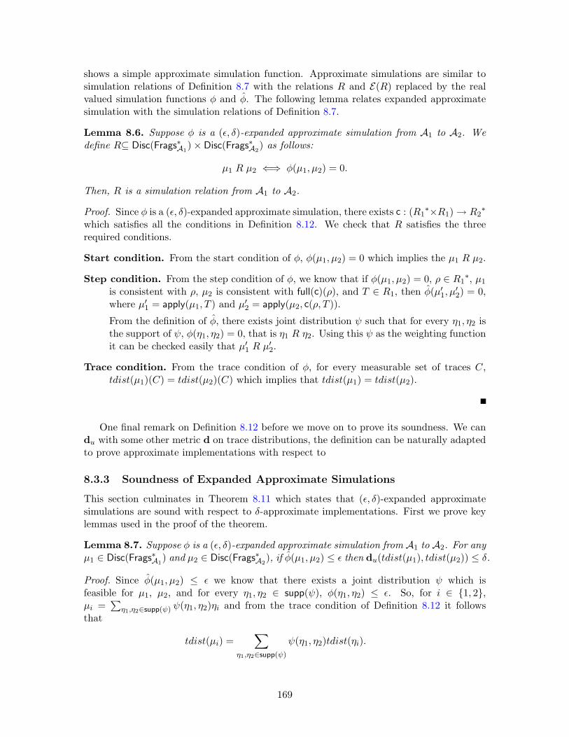
shows a simple approximate simulation function. Approximate simulations are similar tosimulation relations of Definition 8.7 with the relations R and E(R) replaced by the realvalued simulation functions φ and φ. The following lemma relates expanded approximatesimulation with the simulation relations of Definition 8.7.
Lemma 8.6. Suppose φ is a (ε, δ)-expanded approximate simulation from A1 to A2. Wedefine R⊆ Disc(Frags∗A1
)× Disc(Frags∗A2) as follows:
µ1 R µ2 ⇐⇒ φ(µ1, µ2) = 0.
Then, R is a simulation relation from A1 to A2.
Proof. Since φ is a (ε, δ)-expanded approximate simulation, there exists c : (R1∗×R1) → R2
∗
which satisfies all the conditions in Definition 8.12. We check that R satisfies the threerequired conditions.
Start condition. From the start condition of φ, φ(µ1, µ2) = 0 which implies the µ1 R µ2.
Step condition. From the step condition of φ, we know that if φ(µ1, µ2) = 0, ρ ∈ R1∗, µ1
is consistent with ρ, µ2 is consistent with full(c)(ρ), and T ∈ R1, then φ(µ′1, µ′2) = 0,
where µ′1 = apply(µ1, T ) and µ′2 = apply(µ2, c(ρ, T )).
From the definition of φ, there exists joint distribution ψ such that for every η1, η2 isthe support of ψ, φ(η1, η2) = 0, that is η1 R η2. Using this ψ as the weighting functionit can be checked easily that µ′1 R µ′2.
Trace condition. From the trace condition of φ, for every measurable set of traces C,tdist(µ1)(C) = tdist(µ2)(C) which implies that tdist(µ1) = tdist(µ2).
One final remark on Definition 8.12 before we move on to prove its soundness. We candu with some other metric d on trace distributions, the definition can be naturally adaptedto prove approximate implementations with respect to
8.3.3 Soundness of Expanded Approximate Simulations
This section culminates in Theorem 8.11 which states that (ε, δ)-expanded approximatesimulations are sound with respect to δ-approximate implementations. First we prove keylemmas used in the proof of the theorem.
Lemma 8.7. Suppose φ is a (ε, δ)-expanded approximate simulation from A1 to A2. For anyµ1 ∈ Disc(Frags∗A1
) and µ2 ∈ Disc(Frags∗A2), if φ(µ1, µ2) ≤ ε then du(tdist(µ1), tdist(µ2)) ≤ δ.
Proof. Since φ(µ1, µ2) ≤ ε we know that there exists a joint distribution ψ which isfeasible for µ1, µ2, and for every η1, η2 ∈ supp(ψ), φ(η1, η2) ≤ ε. So, for i ∈ 1, 2,µi =
∑η1,η2∈supp(ψ) ψ(η1, η2)ηi and from the trace condition of Definition 8.12 it follows
that
tdist(µi) =∑
η1,η2∈supp(ψ)
ψ(η1, η2)tdist(ηi).
169

We can then express du(tdist(µ1), tdist(µ2)) as follows:
supC∈FTraces∗A
| tdist(µ1)(C)− tdist(µ2)(C)|
= supC∈FTraces∗A
|∑η1,η2
ψ(η1, η2)tdist(η1)(C)−∑η1,η2
ψ(η1, η2)tdist(η2)(C)|
≤ supC∈FTraces∗A
∑η1,η2
ψ(η1, η2)|(tdist(η1)(C)− tdist(η2)(C))|.
For any η1, η2 ∈ supp(ψ), φ(η1, η2) ≤ ε and since φ is an (ε, δ)-expanded approximatesimulation, du(tdist(η1), tdist(η2)) ≤ δ. From Definition 8.8, it follows that | tdist(η1)(C)−tdist(η2)(C)| ≤ δ. Therefore, we have du(tdist(µ1), tdist(µ2)) ≤
∑η1,η2
ψ(η1, η2)δ ≤ δ.
Lemma 8.8. Suppose φ : Disc(X1) × Disc(X2) → R≥0 ∪ ∞ is a function, µi ∈ Disc(Xi)for i ∈ 1, 2, φ(µ1, µ2) ≤ ε with optimal distribution ψ. Let fi : Disc(Xi) → Disc(Xi) bedistributive functions, for i ∈ 1, 2. If for each κ1, κ2 ∈ supp(ψ), φ(f1(κ1), f2(κ2)) ≤ ε,then φ(f1(µ1), f2(µ2)) ≤ ε.
Proof: For each κ1, κ2 ∈ supp(ψ), let ψκ1κ2 be the optimal distribution forφ(f1(κ1), f2(κ2)) = ε. We define a joint distribution ψ′ on Disc(X1)× Disc(X2) as follows:
ψ′∆=
∑(κ1,κ2)∈supp(ψ)
ψ(κ1, κ2)ψκ1,κ2 (8.5)
and show that ψ′ is a feasible distribution for f1(µ1) and f2(µ2) and for any η1, η2 ∈ supp(ψ′),φ(η1, η2) ≤ ε.
1. For feasibility of ψ′ we have to show that for i ∈ 1, 2, fi(µi) equals:∑η1∈Disc(X1),η2∈Disc(X2)
ψ′(η1, η2)ηi
=∑
η1∈Disc(X1),η2∈Disc(X2)
∑(κ1,κ2)∈supp(ψ)
ψ(κ1, κ2)ψκ1,κ2(η1, η2)
ηi=
∑(κ1,κ2)∈supp(ψ)
ψ(κ1, κ2)
∑η1∈Disc(X1),η2∈Disc(X2)
ψκ1,κ2(η1, η2)ηi
=
∑(κ1,κ2)∈supp(ψ)
ψ(κ1, κ2)fi(κi) [from feasibility of ψκ1,κ2 ]
= fi
∑(κ1,κ2)∈supp(ψ)
ψ(κ1, κ2)κi
[from distributivity of fi]
= fi(µi) [from feasibility of ψ].
2. For optimality of ψ′ it suffices to show that for all η1, η2 ∈ supp(ψ′), φ(η1, η2) ≤ε. If ψ′(η1, η2) > 0 then from Equation (8.5) it follows that there exists κ1, κ2 ∈
170

supp(ψ) such that ψκ1,κ2(η1, η2) > 0. Since ψκ1,κ2 is a optimal distribution forφ(f1(κ1), f2(κ2)) = ε, from its optimality we know that for any ν1, ν2 ∈ supp(ψκ1,κ2),φ(ν1, ν2) ≤ ε. In particular, η1, η2 ∈ supp(ψκ1,κ2) and so we have φ(η1, η2) ≤ ε.
Lemma 8.9. Let µii∈I be a countable family of discrete probability measures µi ∈ Disc(Frags∗A)and let µ =
∑i∈I λiµi be a convex combination of µi, where
∑i∈I λi = 1. Let T be task
of A. Then apply(µ, T ) =∑
i∈I λi apply(µi, T ).
Proof. Suppose p1 and p2 are the functions used in the definition of apply(µ, T ), and supposefor each i ∈ I, pi1 and pi2 be the functions used in the definition of apply(µi, T ). Fix a finite ex-ecution fragment α. We show that p1(α) =
∑i λip
i1(α) and p2(α) =
∑i λip
i2(α), from which
it follows that apply(µ, T )(α) = p1(α) + p2(α) =∑
i λi(pi1(α) + pi3(α)) =
∑i λi apply(µi, T ).
To prove that p1(α) =∑
i λipi1(α), we consider two cases. If α = α′aq where α′ ∈
supp(µ), a ∈ T , and α′.lstate, a, η) ∈ D, then, by Definition 8.3 p1(α) = µ(α′)η(q) andfor each i ∈ I, pi1(α) = µi(α′)η(q). Thus, p1(α) =
∑i λip
i1(α). Otherwise, again by
Definition 8.3 p1(α) = 0 and for each i ∈ I, pi1(α) = 0, and the result holds trivially.To prove that p2(α) =
∑i λip
i2(α), we consider two cases. If T is not enabled in α.lstate
then, by Definition 8.3, p2(α) = µ(α), and for each i ∈ I, pi2(α) = µi(α). Thus, p2(α) =∑i λip
i2(α). Otherwise, again by Definition 8.3 p2(α) = 0 and for each i ∈ I, pi2(α) = 0,
and the result holds trivially.
Proposition 8.10. Let µii∈I be a countable family of discrete probability measures µi ∈Disc(Frags∗A) and let µ =
∑i∈I λiµi be a convex combination of µi, where
∑i∈I λi = 1.
Let ρ be a finite sequence of tasks. Then apply(µ, ρ) =∑
i∈I λi apply(µi, ρ).
Proof. The proof is by induction on the length of ρ. If ρ is the empty sequence, then for anyη ∈ Disc(Frags∗A), apply(η, ρ) = η and it follows that µ =
∑i∈I λiµi =
∑i∈I λi apply(µi, ρ).
For the induction step, let ρ = ρ′T . By Definition 8.3, apply(µ, ρ′T ) = apply(apply(µ, ρ′), T ).By the induction hypothesis, apply(µ, ρ′) =
∑i λi apply(µi, ρ′) and thus, apply(µ, ρ′T ) =
apply(∑
i λi apply(µi, ρ′), T ). For each i ∈ I, apply(µi, ρ′) is a discrete probability measurein Disc(Frags∗A). By Lemma 8.9, apply(
∑i λi apply(µi, ρ′), T ) =
∑i λi apply(apply(µi, ρ′), T ).
Using Definition 8.3 it follows that apply(µ, ρ′T ) =∑
i λi apply(µi, ρ′T ) as required.
Theorem 8.11. Let A1 and A2 be two closed comparable task-PIOAs. If there exists a(ε, δ)-expanded approximate simulation function from A1 to A2 then A1 ≤δ A2.
Proof. Let φ be the assumed (ε, δ)-expanded approximate simulation function from A1 toA2. Let µ1 be the probabilistic execution of A1 generated by the starting distributionν1 and a (finite or infinite) task schedule T1, T2, . . .. For each i > 0, we define ρi to bec(T1 . . . Ti−1, Ti). Let µ2 be the probabilistic execution of A2 generated by ν2 and theconcatenation ρ1, ρ2, . . .. It suffices to show that: du(tdist(µ1), tdist(µ2)) ≤ δ.
For each j ≥ 0, let us define µ1,j∆= apply(ν1, T1, . . . , Tj) and µ2,j
∆= apply(ν2, ρ1, . . . , ρj).For i ∈ 1, 2 and for each j ≥ 0, µi,j ≤ µi,j+1 and limj→∞ µi,j = µi. (the above usesLemma 8.20 of Appendix 8.8). Observe that for every j ≥ 0, µ1,j+1 = apply(µ1,j , Tj+1) andalso that µ2,j+1 = apply(µ2,j , ρj+1).
Step 1. We prove by induction that for all j ≥ 0, φ(µ1,j , µ2,j) ≤ ε.
Step 1a. For j = 0, µ1,0 = ν1 and µ2,0 = ν2. By the start condition of the simulationfunction, φ(µ1,0, µ2,0) ≤ ε and therefore by Proposition 8.4 φ(µ1,0, µ2,0) ≤ ε.
171
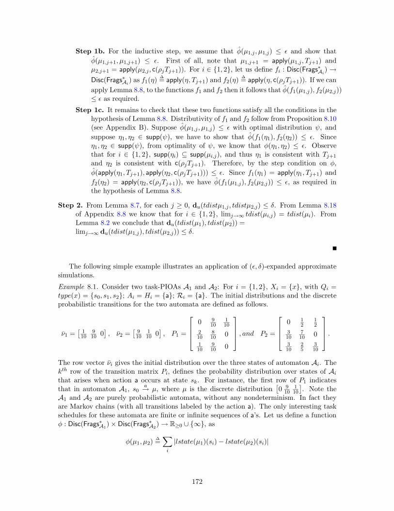
Step 1b. For the inductive step, we assume that φ(µ1,j , µ1,j) ≤ ε and show thatφ(µ1,j+1, µ1,j+1) ≤ ε. First of all, note that µ1,j+1 = apply(µ1,j , Tj+1) andµ2,j+1 = apply(µ2,j , c(ρjTj+1)). For i ∈ 1, 2, let us define fi : Disc(Frags∗Ai
) →Disc(Frags∗Ai
) as f1(η)∆= apply(η, Tj+1) and f2(η)
∆= apply(η, c(ρjTj+1)). If we canapply Lemma 8.8, to the functions f1 and f2 then it follows that φ(f1(µ1,j), f2(µ2,j))≤ ε as required.
Step 1c. It remains to check that these two functions satisfy all the conditions in thehypothesis of Lemma 8.8. Distributivity of f1 and f2 follow from Proposition 8.10(see Appendix B). Suppose φ(µ1,j , µ1,j) ≤ ε with optimal distribution ψ, andsuppose η1, η2 ∈ supp(ψ), we have to show that φ(f1(η1), f2(η2)) ≤ ε. Sinceη1, η2 ∈ supp(ψ), from optimality of ψ, we know that φ(η1, η2) ≤ ε. Observethat for i ∈ 1, 2, supp(ηi) ⊆ supp(µi,j), and thus η1 is consistent with Tj+1
and η2 is consistent with c(ρjTj+1). Therefore, by the step condition on φ,φ(apply(η1, Tj+1), apply(η2, c(ρjTj+1))) ≤ ε. Since f1(η1) = apply(η1, Tj+1) andf2(η2) = apply(η2, c(ρjTj+1)), we have φ(f1(µ1,j), f2(µ2,j)) ≤ ε, as required inthe hypothesis of Lemma 8.8.
Step 2. From Lemma 8.7, for each j ≥ 0, du(tdistµ1,j , tdistµ2,j) ≤ δ. From Lemma 8.18of Appendix 8.8 we know that for i ∈ 1, 2, limj→∞ tdist(µi,j) = tdist(µi). FromLemma 8.2 we conclude that du(tdist(µ1), tdist(µ2)) =limj→∞ du(tdist(µ1,j), tdist(µ2,j)) ≤ δ.
The following simple example illustrates an application of (ε, δ)-expanded approximatesimulations.
Example 8.1. Consider two task-PIOAs A1 and A2: For i = 1, 2, Xi = x, with Qi =type(x) = s0, s1, s2; Ai = Hi = a; Ri = a. The initial distributions and the discreteprobabilistic transitions for the two automata are defined as follows.
ν1 =[
110
910 0
], ν2 =
[910
110 0
], P1 =
0 9
10110
210
810 0
110
910 0
, and P2 =
0 1
212
310
710 0
310
25
310
.The row vector νi gives the initial distribution over the three states of automaton Ai. Thekth row of the transition matrix Pi, defines the probability distribution over states of Aithat arises when action a occurs at state sk. For instance, the first row of P1 indicatesthat in automaton A1, s0
a→ µ, where µ is the discrete distribution[0 9
10110
]. Note the
A1 and A2 are purely probabilistic automata, without any nondeterminism. In fact theyare Markov chains (with all transitions labeled by the action a). The only interesting taskschedules for these automata are finite or infinite sequences of a’s. Let us define a functionφ : Disc(Frags∗A1
)× Disc(Frags∗A2) → R≥0 ∪ ∞, as
φ(µ1, µ2)∆=∑i
|lstate(µ1)(si)− lstate(µ2)(si)|
172

Recall that lstate(µ1) denotes the lstate distribution corresponding to the distribution µ1.Informally, φ measures the L1 distance between the distribution over the states of A1 andA2. It is routine to check analytically that φ satisfies the start condition and the stepcondition of Definition 8.12 for any ε ≥ φ(ν1, ν2) = 1.6 (the trace condition holds trivially).Figure 8-2 confirms this; it shows the lstate distributions of µ1k and µ2k and the values ofφ(µ1k, µ2k), where µik = apply(νi, ak).
0 1 2 3 4 5 6 7 8 9 100
0.2
0.4
0.6
0.8
1
1.2
1.4
1.6
Steps
φ(μ1,μ2)
lstate(μ1)(s0)
lstate(μ1)(s1)
lstate(μ1)(s2)
lstate(μ2)(s0)
lstate(μ2)(s1)
lstate(μ2)(s2)
Figure 8-2: Discrepancy and lstate distributions for A1 and A2.
8.3.4 Need for Expansion
In the step condition in the definition of EAS (Definition 8.12) it is required that ifφ(µ1, µ2) ≤ ε then φ(µ′1, µ
′2) ≤ ε. Indeed, if we replace this condition with the stronger
condition—if φ(µ1, µ2) ≤ ε then φ(µ′1, µ′2) ≤ ε—the resulting approximate simulation func-
tions that we would obtain would be sound for proving approximate implementations. Infact this would have been sufficient for proving approximate implementation in Example 8.1.However, such non-expanded approximate simulation functions are considerably less pow-erful than EASs.
The key motivation for generalizing simulation relations to their current expanded form,first came from the verification of the Oblivious Transfer protocol in [CCK+06d]. In whatfollows, we describe an example from [CCK+06a], adapted to our setting, to illustrate thatallowing φ in the definition of EAS gives it more power.
Example 8.2. Consider the Rand automaton of Figure 8-3 (left). When the choose actionoccurs at state r0, it assigns a number between 1 and n to the variable z, where n is aeven. The initial value of z is ⊥ and the choice is made uniformly at random. The Trapdoorautomaton assigns a random number between 1 and n to the variable y, but in this case theprobabilities are slightly different. The first n
2 numbers are chosen with probability 1n − ε
and the remaining are chosen with probability 1n + ε, where ε 2
n . The comp action ofTrapdoor then applies a known permutation (e.g., if y = n− 1 then z = n, else z = (y + 1)
173
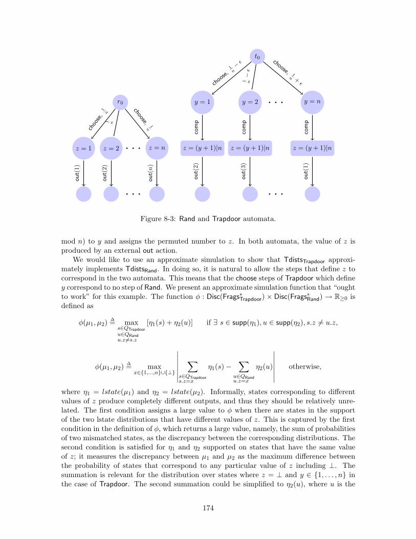
r0
z = 1 z = 2 . . . z = n
. . .
choo
se,
1n
1 n
choose,1n
out(
1)
out(
2)
out(
n)
t0
y = 1 y = 2 y = n. . .
. . .
z = (y + 1)|n z = (y + 1)|n z = (y + 1)|n
choo
se,1n− ε
1 n−
ε
choose, 1n +
ε
com
p
com
p
com
p
out(
2)
out(
3)
out(
1)
Figure 8-3: Rand and Trapdoor automata.
mod n) to y and assigns the permuted number to z. In both automata, the value of z isproduced by an external out action.
We would like to use an approximate simulation to show that TdistsTrapdoor approxi-mately implements TdistsRand. In doing so, it is natural to allow the steps that define z tocorrespond in the two automata. This means that the choose steps of Trapdoor which definey correspond to no step of Rand. We present an approximate simulation function that “oughtto work” for this example. The function φ : Disc(Frags∗Trapdoor) × Disc(Frags∗Rand) → R≥0 isdefined as
φ(µ1, µ2)∆= maxs∈QTrapdoor
u∈QRandu.z 6=s.z
[η1(s) + η2(u)] if ∃ s ∈ supp(η1), u ∈ supp(η2), s.z 6= u.z,
φ(µ1, µ2)∆= maxx∈1,...,n∪⊥
∣∣∣∣∣∣∣∑
s∈QTrapdoors.z=x
η1(s)−∑
u∈QRandu.z=x
η2(u)
∣∣∣∣∣∣∣ otherwise,
where η1 = lstate(µ1) and η2 = lstate(µ2). Informally, states corresponding to differentvalues of z produce completely different outputs, and thus they should be relatively unre-lated. The first condition assigns a large value to φ when there are states in the supportof the two lstate distributions that have different values of z. This is captured by the firstcondition in the definition of φ, which returns a large value, namely, the sum of probabilitiesof two mismatched states, as the discrepancy between the corresponding distributions. Thesecond condition is satisfied for η1 and η2 supported on states that have the same valueof z; it measures the discrepancy between µ1 and µ2 as the maximum difference betweenthe probability of states that correspond to any particular value of z including ⊥. Thesummation is relevant for the distribution over states where z = ⊥ and y ∈ 1, . . . , n inthe case of Trapdoor. The second summation could be simplified to η2(u), where u is the
174

unique state of Rand at which u.z = x.Now we attempt to show that φ is a (2ε, 2ε)-simulation from Trapdoor to Rand without
using the expanded version φ of φ. The task correspondence mapping c : R∗Trapdoor ×
RTrapdoor → R∗Rand as follows:
c(ρ, choose) = λ,
If ρ contains choose then c(ρ, comp) = choose, otherwise c(ρ, comp) = λ,
c(ρ, out) = out
We check the start condition and the step condition for the interesting distributions thatRand and Trapdoor give rise to; the trace conditions can be checked easily from the discrep-ancy between the probabilistic executions.
Let µ11 = apply(δt0 , choose) and µ21 = apply(δr0 , λ) = δr0 . For all s ∈ supp(lstate(µ11)),s.z = t0.z = ⊥, and all u ∈ supp(lstate(µ21)), u.z = r0.z = ⊥. Hence by the secondcondition in the definition of φ, φ(µ11, µ21) = 0 ≤ ε.
Let µ12 = apply(µ11, choose) and µ22 = apply(µ21, λ) = µ21 = δr0 . For all s ∈supp(lstate(µ12)), s.y ∈ 1, . . . , n and s.z is still ⊥. And for all u ∈ supp(lstate(µ22)),u.z = ⊥. Hence, again, the second condition in the definition of φ applies, and
φ(µ12, µ22) =∣∣∣∣( 1n
+ ε+1n
+ ε+ . . .+1n− ε+
1n− ε
)− 1∣∣∣∣ = 0 ≤ ε.
Next, let µ13 = apply(µ12, comp) and µ23 = apply(µ22, choose). Then, there exists s ∈supp(µ13) and u ∈ supp(µ23), such that s.z 6= u.z, and by the first condition, φ(µ12, µ22) =2n + ε > 2ε. Therefore, φ is not a (2ε, 2ε)-approximate (unexpanded) simulation, and wecannot use φ to prove that Trapdoor is a good approximate implementation for Rand, atleast not without using the expanded version of φ.
δy=1,z=2 δy=2,z=3 δy=3,z=4 δy=4,z=1
δz=114
δz=214 − ε ε
δz=314 − ε ε
δz=414
Table 8.1: Optimal joint distribution ψ.
We show that φ can be used as an expanded approximate simulation function. Inparticular, we show that φ(µ13, µ23) ≤ 2ε, and we will use the witnessing joint distributionshown in the table of Table 8.2. Notice that the marginal distributions of ψ match withµ13 and µ23. Further, for any ν1, ν2 in the support of ψ, ν1 and ν2 have the followingproperties: either (i) they are Dirac masses at states that have the same value of z, inwhich case φ(ν1, ν2) = ε from the second condition in the definition of φ, otherwise (ii) forany s ∈ QTrapdoor and u ∈ QRand, ν1(s) ≤ ε and ν2(u) ≤ ε, and therefore by the firstcondition φ(ν1, ν2) ≤ 2ε. It follows that φ(µ13, µ23) ≤ 2ε.
175

By a similar argument it can be checked that φ(µ14, µ24) ≤ 2ε, where µ14 = apply(µ13, out)and µ24 = apply(µ23, out). This covers all the interesting cases and establishes that φ is a(2ε, 2ε)-expanded approximate simulation from Trapdoor to Rand.
8.3.5 Probabilistic Safety
In this subsection, we show how approximate implementations can be used for probabilis-tically reasoning about properties of trace distributions. Let (Traces,FTraces) be the mea-surable space of traces containing the traces of comparable task-PIOAs A1 and A2, andf : (Traces,FTraces) → (Y,FY ) be a measurable function. For example, if Y = 0, 1, thenf could be a predicate on traces that we are interested in proving. For instance, we candefine f(β) to be 0 if a certain undesirable external action a occurs in β, and 1 otherwise.In general, f defines a property of traces that we are interested in verifying. Since f isa measurable function, it is actually a Y -valued random variable on Traces. We use thecustomary notation [f = y] ∆= β ∈ Traces | f(β) = y, for any y ∈ Y .
Lemma 8.12. Let f be a measurable function (random variable) from (Traces,FTraces) to(Y,FY ). Suppose A1 ≤δ A2 and there exists 0 ≤ p ≤ 1 such that for every µ2 ∈ tdists(A2),µ2([f = y]) ≤ p, for some y ∈ Y . Then, for all µ1 ∈ tdist(A1), µ1([f = y]) ≤ δ + p.
Proof. Fix µ1 ∈ TdistsA1 . Since A1 ≤δ A2, from Definition 8.9, we know that there existsµ2 ∈ tdists(A2), such that du(µ1, µ2) ≤ δ. We know that supC∈FTraces
|µ2(C)− µ1(C)| ≤ δ.In particular, |µ1([f = y])−µ2([f = y])| ≤ δ. As µ2([f = y]) ≤ p, we have µ1([f = y]) ≤ p+δas required.
Suppose that A2 triggers the “bad” action a with probability at most p. Formally, thismeans that the probability of any trace containing a, according to any trace distributionof A2, is at most p. If A1 and A2 are comparable closed task-PIOAs such that A1 ≤δ A2,then from the Lemma 8.12 we can conclude that A1 triggers action a with probability atmost p+ δ.
Violation of safety properties can also modeled as trace functions. Assume that violationof some safety property S is indicated by the occurrence of one of the external actions fromthe set U ⊆ E1 = E2. We define the function f : Traces → 0, 1 as f(β) ∆= 0 if some actionfrom U occurs in the trace β, otherwise f(β) ∆= 1. It can be easily checked that f is ameasurable function and therefore is a boolean valued random variable. The event [f = 0]corresponds to the set of traces in which S is violated. Now, if we know that in any tracedistribution of A2 the probability of any U occurring is at most p and that A1 ≤δ A2, thenfrom Lemma 8.12 we can conclude that in any trace distribution of A1 the probability ofoccurrence of U , and hence the violation of S, is at most δ + p.
8.4 Discounted Uniform Approximate Implementation
In the preceding section we defined uniform approximate implementation for PIOAs andproved that expanded approximate simulations are sound for proving this implementationrelationship. We also demonstrated that uniform approximate implementations are suitablefor probabilistically reasoning about certain classes of properties, like safety properties,where it is sufficient to quantify the absolute discrepancy in the trace distributions overall sets of traces. For certain other classes of properties the uniform metric is not suitable,
176

because the worst case discrepancy over all sets of traces does not convey useful information.We illustrate this with the following example.
Example 8.3. This example is the untimed version of Example 7.3 and models Ben-Or’srandomized consensus protocol [BO83] for n fault-prone processors to agree on a valid value.The algorithm proceeds in a sequence of stages in each of which nonfaulty processes sendand receive messages based on coin-flips and comparison of values. If the processes haveaccess to perfectly random coins, then with some probability p, a stage ends successfullyand all nonfaulty processes agree on a value, and after one communication round of asuccessful stage the consensus value is disseminated. An unsuccessful stage is followed bythe beginning of the next stage.
The automaton in Figure 8-4 captures the termination behavior of the algorithm. Theprotocol starts in state s10 (corresponds to the states with phase = 0, stage = 1 of au-tomaton Consensus of Example 7.3). The starting state for the successive stages are thestates s20, s30, . . .. If the the ith stage completes successfully then state si1 is reached. Theaction try models the computation and communication within a stage. From stage si0,with probability p it leads to s(i+1)0, the next stage, and with probability 1− p it leads tosi1. The action decide marks the termination of the protocol and it takes si1 to si2 withprobability 1.
s10
s11
s12
s20
s21
s22
s30
s31
s32
s40
s41
s42
. . .
try,
1−
pdec
ide
try, p
try,
1−
pdec
ide
try, p
try,
1−
pdec
ide
try, p
try,
1−
pdec
ide
try, p
Figure 8-4: Automata representing Ben-Or consensus protocol.
Suppose PIOA A1 is an instance of the automaton in Figure 8-4 with perfect randomcoins, that is, p = 1 − 1
2n and 1 − p = 12n . Let A2 be a task-PIOA instance of the same
automaton with slightly biased coins. We model the transition probabilities for A2 by p+ εand 1−p−ε, for a small positive ε. We would like to compare the probabilities of terminationof A1 and A2 after a certain number of rounds, say k. With the uniform approximateimplementation, we can show that the difference in these probabilities is less than δ, for afixed δ > 0. However, if individual probabilities of termination are themselves less than δthen this δ-approximation is too coarse and does not give us any useful information.
8.4.1 Discounted Uniform Metric on Traces
In the remainder of this section, we show how a discounted version of the uniform metriccan be used to make more finer-grained comparison of probabilities of traces.
Definition 8.13. A probability distribution µ on execution fragments of A is said to be
177
finite if Frags∗A is a support for µ. A trace distribution µ of A is finite if Traces∗A is a supportfor µ.
Since any set of finite execution fragments is measurable, any finite probability distri-bution on execution fragments of A can also be viewed as a discrete probability measure onFrags∗A. Likewise, a finite trace distribution can be viewed as a discrete distribution overTraces∗A. In this section, we consider task-PIOAs with finite (trace) distributions and willtreat these distributions as discrete distributions on execution fragments or traces.
Definition 8.14. For any k ∈ N, the kth uniform metric is a function dk : Disc(TracesA)×Disc(TracesA) → R≥0 defined as:
dk(µ1, µ2)∆= max
β∈E∗,|β|=k|µ1(β)− µ2(β)|.
The kth uniform metric measures the discrepancy between two trace distributions bylooking at traces of length k only. We show that dk is a pseudometric and that it satisfiesthe convergence property stated in Lemma 8.2.
Proposition 8.13. For all k ∈ N, dk is a pseudometric.
Proof. The symmetry property is easy to check. We prove that dk satisfies the triangleinequality. Let µ1, µ2, µ3 be distributions on E∗. dk(µ1, µ3) = maxβ∈E∗,|β|=k |µ1(β)−µ3(β)|.Suppose β3 is a trace that realizes the supremum.
|µ1(β3)− µ3(β3)| ≤ |µ1(β3)− µ2(β3)|+ |µ2(β3)− µ3(β3)|dk(µ1, µ3) ≤ max
β,|β|=k|µ1(β)− µ2(β)|+ max
β,|β|=k|µ2(β)− µ3(β)|,
≤ dk(µ1, µ2) + dk(µ2, µ3).
Lemma 8.14. Suppose A1 and A2 are closed task-PIOAs. For i ∈ 1, 2, let µijj∈N be achain of discrete probability distributions on the traces of Ai and let limj→∞ µij = µi. Thenfor any k ∈ N, limj→∞ dk(µ1j , µ2j) = dk(µ1, µ2).
Proof. The proof is the same as the proof of Lemma 8.2 for the du metric.
Given a family of positive discount factors δkk∈N, we say that task-PIOA A1 δk-implements A2, if one-sided Hausdorff distance from TdistsA1 to TdistsA2 is at most δk, forevery k ∈ N.
Definition 8.15. Suppose A1 and A2 are comparable, closed task-PIOAs and δkk∈N isa collection of positive real numbers, called discount factors. If for every trace distributionµ1 inTdistsA1 there exists a trace distribution µ2 ∈ TdistsA2 such that for every k ∈ N,dk(µ1, µ2) ≤ δk, then we say that A1 δk-implements A2 and write this as A1 ≤δk A2. A1
and A2 are said to be δk-equivalent , written as A1∼=δk A2, if A1 ≤δk A2 and A2 ≤δk A1.
178

8.4.2 Discounted Approximate Simulation
We define a new kind of approximate simulation called Discounted Approximate Simula-tion (DAS) for proving discounted approximate implementations for task-PIOAs. Givena distribution µ over executions (or traces) we denote the longest execution (respectivelytrace) in the support of µ by L(µ). We extend this notation to a pair of distributions,L(µ1, µ2)
∆= max(L(µ1), L(µ2)), that is, it is the length of longest execution in the supportof either µ1 or µ2.
Definition 8.16. Suppose A1 and A2 are two comparable closed task-PIOAs, and φkk∈Nis a collection of functions, where each φk : Disc(Frags∗A1
) × Disc(Frags∗A2) → R≥0 ∪ ∞.
Given a collection of real number pairs εk, δkk∈N, the collection φk is an (εk, δk)-discounted approximate simulation from A1 to A2 if there exists a function c : R∗1×R1 → R∗2such that the following properties hold:
1. (Start condition) φ0(ν1, ν2) ≤ ε0.
2. (Step condition) If for all k ≤ L(µ1, µ2), φk(µ1, µ2) ≤ εk, T ∈ R1, ρ ∈ R∗1, µ1 isconsistent with ρ, and µ2 is consistent with full(c)(ρ), then for all k ≤ L(µ′1, µ
′2),
φk(µ′1, µ′2) ≤ εk, where µ′1 = apply(µ1, T ) and µ′2 = apply(µ2, c(ρ, T )).
3. (Trace condition) If for all k ≤ L(µ1, µ2), φk(µ1, µ2) ≤ εk then for allk ≤ L(tdist(µ1), tdist(µ2)) dk(tdist(µ1), tdist(µ2)) ≤ δk.
A family of functions φk is an (εk, δk) discounted approximate simulation if (i) Theinitial distributions ν1 and ν2 are ε0-close in the sense of φ0. (ii) Suppose two distribu-tions µ1, µ2 are εk-close in the sense of φk, for every k ≤ L(µ1, µ2). then the distributionsµ′1—obtained by applying a new task to µ1, and µ′2—obtained by applying a correspondingsequence of tasks to µ2, are also εk-close in the sense of φk, for every k ≤ L(µ′1, µ
′2). (iii) Fi-
nally, if µ1, µ2 are εk-close in the sense of φk, for every k ≤ L(µ1, µ2). then the correspondingtrace distributions are δk-close in the sense of dk for every k ≤ L(tdist(µ1), tdist(µ2)). Ex-ample 8.1 shows a simple approximate simulation function. Approximate simulations aresimilar to simulation relations of Definition 8.7 with the relations R and E(R) replaced bythe real valued simulation functions φ and φ.
Note that although we have not the expanded version of the φk’s in defining the stepcondition, it might be possible to obtain more powerful expanded discounted approximatesimulations by changing the requirement φk(µ′1, µ
′2) ≤ εk to φk(µ′1, µ
′2) ≤ εk .
8.4.3 Soundness of Discounted Approximate Simulation
We prove Theorem 8.15 which states that (εk, δk)- approximate simulations are sound withrespect to δk-approximate implementations.
Theorem 8.15. Let A1 and A2 be two closed isomorphic comparable task-PIOAs. If thereexists a (εk, δk)-discounted approximate simulation function from A1 to A2 then A1 ≤δk A2.
Proof. Let φ be the assumed (εk, δk)-discounted approximate simulation function fromA1 toA2. Let µ1 be the probabilistic execution of A1 generated by the starting distribution ν1 anda finite task schedule T1, T2, . . . , Tn. For each i > 0, we define ρi to be c(T1 . . . Ti−1, Ti). Letµ2 be the probabilistic execution of A2 generated by ν2 and the concatenation ρ1, ρ2, . . . , ρn.It suffices to show that dw(tdist(µ1), tdist(µ2)) ≤ δ.
179

For each j ≥ 0, let us define µ1,j∆= apply(ν1, T1, . . . , Tj) and µ2,j
∆= apply(ν2, ρ1, . . . , ρj).For i ∈ 1, 2 and for each j ≥ 0, µi,j ≤ µi,j+1 and µi,n = µi. Observe that for every j ≥ 0,µ1,j+1 = apply(µ1,j , Tj+1) and µ2,j+1 = apply(µ2,j , ρj+1).
We prove by induction that for all j ≥ 0, for all k ≤ L(µ1,j , µ2,j), φk(µ1,j , µ2,j) ≤ εk.For j = 0, µ1,0 = ν1 and µ2,0 = ν2. By the start condition of the simulation func-tion, φ0(µ1,0, µ2,0) ≤ ε. For the inductive step, we assume that for all k ≤ L(µ1,j , µ2,j),φk(µ1,j , µ2,j) ≤ εk. Then, from Part (ii) of Definition 8.12 it follows that for all k ≤L(µ1,j+1, µ2,j+1), φk(µ1,j+1, µ2,j+1) ≤ εk. In particular, for all k ≤ L(µ1, µ2), φk(µ1, µ2) ≤εk, from which, using condition (iii) it follows that for all k ≤ L(tdist(µ1), tdist(µ2)),dk(tdist(µ1), tdist(µ2)) ≤ δk.
Example 8.4. (Continuation of Example 8.3.) Let εk = δk = (p+ ε)k − pk, for each k ∈ N.We will show that A1 and A2 are δk-equivalent using the following discounted approximatesimulation:
for each k, φk(µ1, µ2) = maxα,anum(α)=k|µ1(α)− µ2(α)|, (8.6)
where µ1 ∈ Disc(Execs∗A1), µ2 ∈ Disc(Execs∗A2
), and anum(α) is the number of occurrence ofthe action try in the execution α.
Proposition 8.16. The collection of functions φk defined above is indeed an (εk, δk)-discounted approximate simulation from A1 to A2.
Proof sketch. We check that the collection φk satisfies the three conditions in Defini-tion 8.16.
Start condition. ν1 = ν2 = δs10 , and therefore φ0(ν1, ν2) = 0.
Step condition. We define the task correspondence function in the obvious way, c(ρ, T ) ∆=T , where ρ is a task schedule and T is a task for A1. Thus for any µ1 ∈ Disc(Execs∗A1
)and µ2Disc(Execs∗A2
) that are obtained from ν1 and ν2 by applying a sequence of tasks,L(µ1, µ2) = L(µ1) = L(µ2). Consider any µ1 ∈ Disc(Execs∗A1
),µ2 ∈ Disc(Execs∗A2),
and suppose µ1 = apply(ν1, ρ) and µ2 = apply(ν2, full(c)(ρ)). Let us denote µ′1 =apply(µ1, T ), and µ′2 = apply(µ2, c(ρ, T )) = apply(µ2, T ). Then, it suffices to showthat for all k ≤ L(µ1, µ2), φk(µ′1, µ
′2) ≤ (p + ε)k − εk. This part of the proof is by a
case analysis on the types of tasks, T = try, decide and the types of executions.
The interesting cases are for T = try and executions of the form α = α′ try sk0or α = α′try s(k−1)1, for some k ≤ L(µ1). For the first case, µ′1(α) = µ1(α′)p andµ′2(α) = µ2(α′)(p + ε), and therefore φk+1(µ′1, µ
′2) = p|µ2(α′) − µ1(α′)| + εµ2(α′).
From the inductive hypothesis, |µ2(α′)− µ1(α′)| ≤ εk. It follows that, φk+1(µ′1, µ′2) ≤
p|(p+ ε)k − pk|+ ε(p+ ε)k ≤ εk+1. Likewise in the second case, µ′1(α) = µ1(α′)(1− p)and µ′2(α) = µ2(α′)(1− p− ε), and performing a similar calculation as above, we canshow that φk+1(µ′1, µ
′2) ≤ εk.
Trace condition. First of all, for any µ1 ∈ Disc(Execs∗A1) that are obtained from ν1 by
applying a sequence of tasks, L(µ1) = L(tdist(µ1)). If β is a trace of the formakd, for some k ≥ 0. Then, for i ∈ 1, 2, tdist(µi)(β) = µi(α), where α =s10as20 . . . sk0trysk1decidesk2. From which it follows that |tdist(µ1)(β)−tdist(µ2)(β)| =|µ1(α) − µ2(α)| ≤ φk+1(µ1, µ2) ≤ εk+1. On the other hand, if β is a trace of the
180

form ak+1, for some k ≥ 0. Then, for i ∈ 1, 2, tdist(µi)(β) = µi(α1) + µi(α2),where α1 = s10 try s20 . . . s(k+1)0 try s(k+1)1 and where α2 = s10 try s20 . . . s(k+2)0.Thus, |tdist(µ1)(β)− tdist(µ2)(β)| = |µ1(α1) + µ1(α2)− µ1(α1)− µ2(α1)| = |µ1(α)−µ1(α)|, where α = s10 try s20 . . . s(k+1)0. Therefore, |tdist(µ1)(β) − tdist(µ2)(β)| ≤φk+1(µ1, µ2) ≤ εk+1 as required.
8.5 Approximations for Task-PIOAs
In this section, we discuss how the notion of uniform approximate implementations andthe soundness of EASs extendeds to general (not necessarily closed) task-PIOAs. In ananalogous manner, discounted approximate implementation and DAS can also be extended.
The basic idea is to define a new notion of implementation following the approachof [CCK+06a]. As we defined external behavior in the case of PTIOAs, we formulate theexternal behavior of a task-PTIOA A as a mapping from possible “environments” for A tosets of trace distributions that can arise when A is composed with the given environment.
Definition 8.17. An environment for task-PIOA A is a task-PIOA E such that the com-position of A and E is closed.
Definition 8.18. The external behavior of a task-PIOAA, written as ExtBehA, is a functionthat maps each environment task-PIOA E for A to the set of trace distributions of thecomposition of A and E .
Approximate implementation for general task-PIOAs can then be defined to be closenessof external behavior for all environments.
Definition 8.19. If A1 and A2 are comparable then A1 is said to δ-implement A2, for someδ ≥ 0, if for every environment task-PIOA E for bothA1 andA2, for every µ1 ∈ ExtBehA1(E)there exists µ2 ∈ ExtBehA2(E) such that du(µ1, µ) ≤ δ.
Based on this modified definition of approximate implementation the soundness of ex-panded approximate simulations for general task-PIOAs follow as a Corollary to Theo-rem 8.11.
Corollary 8.17. Let A1 and A2 be two comparable task-PIOAs. Suppose that for everyenvironment E for both A1 and A2, there exists a (εE , δ)-approximate simulation functionfrom the composition of A1 and E to the composition of A2 and E. Then A1 ≤δ A2.
8.6 Related Work
A variety of implementation relations have beep proposed in the literature for probabilisticautomata [LS91, LMMS98, CCK+06b, C. 96, SvdS05, BLB05]. These notions of implemen-tation rely on equality of observable behavior. That is, every observable behavior of theconcrete system must be exactly equal to some observable behavior of the abstract spec-ification. The fragility of these equality-based implementation relations have been knownfor quite some time [JS90, DJGP02, GJP04] In [JS90] Jou and Smolka formalized “sim-ilarity” of traces using a metric and developed the corresponding notion of approximateequivalence for probabilistic automata. Approximation metrics for probabilistic systemsin the context of Labelled Markov Processes (LMP) have been extensively investigated
181

and many fundamental results have been obtained by Desharnais, Gupta, Jagadeesan andPanangaden [DJGP02, DGJP03, DGJP04] and by van Breugel, Mislove, Ouaknine, andWorrell [vBW01b, vBMOW03, vBMOW05, MWMW04, MOW04]. The first set of authorsintroduced a Kantorovich-like metric for LMPs and presented the logical characterization ofthis metric. Van Breugel et al. have presented intrinsic characterizations of the topologicalspace induced by the above metric. This characterization is based on a final coalgebra fora functor on the category of metric spaces and nonexpansive maps. Another interestingfacet of this body of work is the polynomial time algorithm for computing the metric pre-sented by van Breugel and Worrell in [vBW01a]. For Generalized Semi-Markov Processes(GSMP) [GJP04], Gupta, Jagadeesan and Panangaden have developed pseudo-metric ana-logues of bisimulation and have shown that certain observable quantitative properties arecontinuous with respect to the introduced metric. Kwiatkowska and Norman have devel-oped the denotational semantics for a divergence-free probabilistic process algebra based ona metric on probability distribution over executions [KN96]. In the non-probabilistic setting,Girard and Pappas [GP05, GJP06] have developed the theory of approximate implemen-tations for Metric Transition Systems (MTS). The state space and the space of externalactions of an MTS are metric spaces. Based on these metrics, the authors develop a hierar-chy of approximation pseudo-metrics between MTSs measuring distance between reachablesets, sets of traces and bisimulations. The authors have also developed algorithms forexactly and approximately computing these metrics.
Our work differs from all of the above in at least one of the following ways: (a) thetask-PIOA model allows both nondeterministic and probabilistic choices, and (b) the im-plementation relation in our framework is based on trace distributions and not bisimilarityof states. Approximate implementation is derived from a metric over trace distributions,and thus, we do not require the state spaces of the underlying automata nor the commonspace of external actions to be metric spaces. Metrics on trace distributions of PIOAs areused by Cheung in [Che06]to show that sets of trace distributions form closed sets in acertain metric space. This result is then used to show that finite tests are sufficient todistinguish between a members of a certain class of PIOAs. The metric used in the abovework is related to our uniform metric but it is defined on the set [0, 1]Traces whereas ouruniform metric is exclusively defined on the set of trace distributions.
8.7 Summary
In this chapter we have introduced the notion of approximate implementations for task-structured probabilistic I/O automata. In particular, we have defined two different kindsof approximate implementations, based on the uniform metric and the discounted uniformmetric on trace distributions of task-PIOAs. We proposed expanded approximate simula-tions and discounted approximate simulations for proving, the two proposed implementationrelations, respectively. EAS and DAS can be used to approximately reason about probabilis-tic safety and termination properties. PIOAs can be nondeterministic and our constructiondoes not require the underlying state spaces of the automata or the space of external actionsto be metric spaces.
In our formulation of expanded approximate simulations, a simulation proof reduces tofinding an optimal joint distribution satisfying certain constrains on the marginals. Thisis closely related to the well known Kantorovich optimal transportation problem [Kan].For well-behaved classes of simulation functions, therefore, we would like to explore the
182

possibility of proving approximate simulations by solving optimization problems.In the future, we want develop a new kind of Discounted Expanded Approximate Simula-
tions that combines the features of EAS and DAS. We would also like to develop simulationbased proof techniques where the simulation functions are functions of distributions overstates and not functions of distributions over execution fragments. Finally, we would like toextend the notion approximate implementations to the Probabilistic Timed I/O Automatonframework 7.
8.8 Appendix: Limits of Chains of Distributions
All the definitions and lemmas in this Appendix are from [CCK+06b]. In this AppendixA will be a task-PIOA. Given a finite execution fragment α of A, the cone of executionsgenerated by this fragment Cα is the set of all execution fragments that extend α. Given afinite trace β of A, Cα is the set of all traces that extend β.
Definition 8.20. If µ1, µ2 ∈ Disc(FragsA), such that for every α ∈ Frags∗A, µ1(Cα) ≤µ2(Cα), then we write µ1 ≤ µ2.
Definition 8.21. A chain of probability measures on execution fragments of A is an infinitesequence µ1, µ2, . . . of probability measures on execution fragments of A such that µ1 ≤µ2 . . .. Given a chain, the limit of the chain is defined as a function µ on the σ-algebragenerated by the cones of execution fragments of A, as follows: for each α ∈ Frags∗A,µ(Cα) ∆= limi→∞ µi(Cα).
Standard measure theoretic arguments guarantee that µ can be extended uniquely to aprobability measure on the σ-field generated by the cones of finite execution fragments.
Definition 8.22. If µ1, µ2 are probability measures on traces of A, such that for everyfinite trace β of A µ1(Cβ) ≤ µ2(Cβ), then we write µ1 ≤ µ2.
Definition 8.23. A chain of probability measures on traces of A is an infinite sequenceµ1, µ2, . . . of probability measures on traces of A such that µ1 ≤ µ2 . . .. Given a chainof probability measure on traces, the limit of the chain is defined as a function µ on theσ-algebra generated by the cones of traces of A, as follows: for each finite trace β of A,µ(Cβ)
∆= limi→∞ µi(Cβ).
Again, µ can be extended uniquely to a probability measure on the σ-field generated bythe cones of finite traces.
Lemma 8.18 (4 of [CCK+06b]). Let µ1, µ2, . . . be a chain of measures on FragsA and letµ = limi→∞ µi, then limi→∞ tdist(µi) = tdist(µ).
Lemma 8.19 (11 of [CCK+06b]). Let µ ∈ Disc(Frags∗A) and σ be a finite task schedule forA. Then apply(µ, ρ) ∈ Disc(Frags∗A).
Lemma 8.20 (20 of [CCK+06b]). Let µ ∈ Disc(Frags∗A) and ρ1, ρ2, . . . be a finite or infinitesequence of task schedulers for A. For each i > 0 let ηi = apply(µ, ρ1ρ2 . . . ρi). Let ρ =ρ1ρ2 . . . be the concatenation of the all the task schedulers, and let η = apply(µ, ρ). Thenthe ηi’s form a chain and η = limi→∞ ηi.
183

Chapter 9
Conclusions
9.1 Evaluation
The objective of this PhD thesis project was to explore a general class of hybrid systemmodels with the purpose of developing specification and verification for embedded softwaresystems that interact with physical processes.
The language proposed here, HIOA, provides structures and compositional semantics forspecifying a very general class of nonprobabilistic hybrid systems. We have found that a vari-ety of system models including vehicle and air-traffic control systems [UL07, MWLF03], car-diac cell models used in systems biology [GMY+07], algorithms for mobile robotics [LMN],real-time and distributed algorithms [FDGL07, ALL+06, CLMT05], can be expressed natu-rally in HIOA . While in the thesis we focused on formal analysis of HIOA specifications, thesespecifications are also amenable to simulation. The TIOA subset of HIOA forms the back-bone of the Tempo toolset [TEM07]. This toolset supports simulation and model checking,in addition to some of the verification techniques presented in the thesis, hence making itpossible to apply different analysis techniques to the same hybrid system specification.
For the majority of the applications we have studied, direct automatic verification wouldbe impossible, and therefore, we decided to focus on verification methods that dependon user guidance. Invariance and implementation verification techniques proposed hererely on inductive properties and simulation relations—which the user has to supply; butonce these are obtained, the desired property can be deduced with relative ease. In fact,our theorem prover interface for HIOA partially, and sometimes completely, automates thisdeduction process. In practice, finding the invariants and checking them is often an iterativeprocess, where one starts by guessing an invariant and then attempts to prove it; if theproof fails then the invariant is refined and so on. This iterative process can be performedmore efficiently using our theorem prover interface because the existing proof script can beexecuted automatically on the modified invariant.
Apart from the case studies presented here, the theorem prover interface has been ap-plied by Umeno [UL07] in a major case study concerning safety verification of an aircraftlanding protocol. This is encouraging, and illustrates that it is possible to model and verifyrealistic hybrid system models in our framework. Constructing proofs, even with the aidour strategies, is not routine and takes significant effort. This is because our strategiesare able to automate only shallow proofs. We expect that new domain-specific strategieswill make the deductive verification practical for hybrid models that have relatively simplecontinuous dynamics.
184
Our optimization-based stability verification approach gives a family of methods inwhich the hardness of the optimization problem that one has to solve (for verifying stability)depends on the complexity of the dynamics of the hybrid model in question. For certainclasses of hybrid systems, this means that stability can be verified automatically usingstandard mathematical programming tools. These types of methods can help us decide onthe subclass of SHIOAs that we should restrict our attention to, while modeling the system,so as to make verification feasible with the available resources.
Techniques for verifying quantitative properties allow us to prove performance (or reli-ability) of a system within the same formal framework is used for proving correctness. Wehave extended the usual notions of implementation for (discrete) probabilistic automata toobtain approximate implementation relations. This lets us quantify how close an imple-mentation is to an ideal specification. We have developed sound simulation-based prooftechniques for establishing these relationships. We have recently used these techniques toverify the statistical zero-knowledge property of a classical authentication protocol [GPS06](not presented in the thesis).
In order to state and verify quantitative properties for hybrid systems we have to in-corporate probabilities in the hybrid system model. This motivated us to develop theProbabilistic Timed I/O Automata model. PTIOAs can model concurrent execution ofcomponents, discrete and continuous evolution, and probabilistic choices based on generalcontinuous probability distributions. In developing semantics PTIOAs we had to first resolvenontrivial measurability related issues and then find a way for resolving nondeterminism.Defining a set of axioms that ensure measurability of reasonable sets of executions andtraces, and adapting the task mechanism of [CCK+06a] for resolving nondeterminism, wewere able to develop trace-based semantics for PTIOAs. Currently PTIOAs provide frame-work for modeling probabilistic hybrid systems that arise in, for example, randomized,real-time algorithms, timing based security protocols, and control systems with noisy sam-pling, but much work remains to be done in developing verification techniques for booleanand quantitative properties.
9.2 Future Directions
The state of research for probabilistic and nonprobabilistic hybrid systems are at two differ-ent levels. The latter being more mature, future efforts should focus on new software toolsfor verification and applications, while in the case of probabilistic hybrid systems emphasisshould be on developing the basic verification techniques.
9.2.1 Modeling Probabilistic Hybrid Systems
We show that the composition of two PTIOAs is also a PTIOA only if the compositeautomaton satisfies an additional measurability requirement, namely, axiom M2. PTIOAswe encountered do satisfy M2, but we would like to define a subclass of PTIOAs that isclosed under composition (without any extra assumptions). For obtaining this propertyit may be necessary to impose restrictions on the trajectories of PTIOAs or to imposeadditional measurability requirements.
A second improvement for the PTIOA framework would be to include input/output vari-ables that will enable component automata to communicate continuously. Including inputvariables pose a technical challenge: in defining the probability measure over executions ofsuch an automaton, the maximal progress assumption implied by time-action determinism
185

D3 will have to be removed. This is because a trajectory, in that case, would determinedonly in part by the state, and it will also depend on the inputs.
Finally, the relative strengths of the different scheduling mechanisms has to be stud-ied. In this thesis we used oblivious task schedulers for resolving external nondeterminismand local schedulers for resolving internal nondeterminism. Other types of schedulers,such as Markovian, history-dependent, and randomized schedulers should be considered forPTIOAs. We can remove the time-action determinism axiom D3 by assuming that eachPTIOA component has a local scheduler, and therefore most of the scheduling conflictsare resolved, except for races. Smolka and Stark [ES03, Sta03], assume that such conflictshappen only with probability 0, and so can be ignored. The trace-based semantics obtainedfor these different scheduling mechanism will no doubt be different from the one we haveproposed. Then, we have to draw a clear recipe of which semantics is suitable for whatapplication domain.
9.2.2 Stability
The definition of stability used in the hybrid systems literature and also in this thesis isstrictly concerned with the continuous state of the system. On the other hand, the notion ofself-stabilization has been widely used in designing distributed algorithms [Dol00, NA02].A distributed algorithm is said to be self-stabilizing if it stabilizes to correct behavior,from an arbitrary state, if the underlying components start “behaving well” from somepoint onward. This is a common notion in algorithms designed for somewhat fault-proneenvironments that must continue operations, even after periods of failures, e.g., the Internet,or a mobile computing system. It is necessary to propose a general definition of stability ofhybrid systems, that encompasses both its discrete and its continuous variables. Theel etal. have recently applied Lyapunov function based techniques for verifying self-stabilizationproperties [DOT06], however, a theory that unifies these two distinct notions of stabilityremains unknown. This generalized notion of stability will enable us to prove stability ofa hybrid system as a whole. Further, we can try to carry the techniques for developingself-stabilizing algorithms, like those in [Dol00], over to designing stable hybrid systemsoperating in uncertain real-world environments. For example, in a mobile network setting,if we lose location information about where nodes are, we can search for them in the realworld, and restore the information to where it belongs.
Extending the the stability verification techniques proposed here to the stochastic settingis a promising direction for future research. Stability conditions for probabilistic switchedsystems using Lyapunov function-like arguments have been derived in [CL06, CL04]. It canbe shown that for certain classes of PTIOAs, the problem of proving almost sure stability ,using these Lyapunov arguments can be formulated as optimization problems that can besolved efficiently. In the simplest case, we consider PTIOAs where the discrete transitionsare triggered by a discrete time Markov chain. That is, the mode switches occur periodicallyevery ∆ time and the new modes is chosen probabilistically. In this simple setting it canbe shown that the Average Dwell Time (ADT) property reduces to detecting the minimumcost cycle in a graph, as in the case of one-clock initialized SHIOAs. It would be interestingto explore similar verification approaches for other, more expressive, classes of probabilistichybrid systems.
186
9.2.3 Approximate Implementations
Research on quantitative and approximate verification techniques is in its early stages andmuch work remains to be done. In the context of discrete probabilistic automata, animmediate research goal, is to develop discounted expanded simulations as a more powerfulsubstitute for the ordinary discounted simulation proposed here.
In our formulation of expanded approximate simulations, a simulation proof reduces tofinding an optimal joint distribution satisfying certain constrains on the marginals. Thisis closely related to the well-known Kantorovich optimal transportation problem [Kan].Exploring the connection between these two problems, it may become possible to proveapproximate simulations by solving optimization problems.
Notions of approximate implementations for probabilistic hybrid will have to be robustwith respect to small perturbations to 1. time of occurrence of events, and also 2. probabilityof occurrence of events. This means that we have to use metrics on trace distributions thattake into account both the differences in timing and probability characteristics. Fortunately,there exists a rich body of literature (see, for example, [Rac91]) that offers many choicesfor such metrics on probability distributions. Based on these metrics we should developnotions of approximate implementation for PTIOAs and simulation-based techniques forestablishing these relationships. The techniques introduced in Chapter 8 will be useful inattacking this problem, but tools from functional analysis will also have to be employedalong the way.
9.2.4 Software Tools
The HIOA -PVS interface enables effective verification of hybrid system models with complexdata-types and logical expressions. However, significant user interaction becomes necessaryfor models with nonlinear algebraic equations. We have to address this issue by developinga verification platform, based on Tempo, that integrates theorem provers, model checkers,computer algebra systems, and mathematical program solvers. As an example of how thesedifferent tools can be utilized with in the same framework, consider the safety and stabilityverification conditions of Chapters 4 and 5. These conditions could be checked by computeralgebra systems and optimization tools, whereupon, these conditions can be used by theoremprover strategies for automatically deducing the properties.
The long-term success of any model-based software development methodology dependson how well marginal efforts in development translate to quantifiable gains in quality . Build-ing coarse models and proving that they roughly conform to an ideal design should berelatively easy; and by refining models, improving designs, and expending extra effort inverification, it should be possible to prove closer conformance, and sharper guarantees. Itis important that we create software development platforms that are recognized to have theabove marginal gain property. Approximate implementations provide one possible basis formeasuring conformance, and it is necessary to develop other, non-probabilistic metrics.
187

List of Symbols and Functions
A ≤ B A implements B, i.e., TracesA ⊆ TracesB, 27
A ≤δ B A δ-approximately implements B w.r.t. uniform metric, 166
A ≤δk B A δk-approximately implements B w.r.t. discounted uniform metric, 178
A ≤switch B A switches slower than B, 80
D Set of discrete transitions of a hybrid automaton, 25
Disc(Q) Set of discrete probability distributions over (Q,FQ), 160
ExecsA Set of all executions of automaton A, 26
ExtBehA External behavior of A, a map from environment(E) to TdistsAE , 151
FragsA Set of all execution fragments of automaton A, 26
M Set of mode switching discrete transitions of a SHIOA, 35
(S,FS) A measurable space on set S; FS is a σ-algebra over S., 136
µx,B If unique action a ∈ B is enabled at x such that x a→ µ, then µx,B = µ, 138
ReachA Set of all reachable states of automaton A, 26
supp(µ) Support of discrete probability measure µ, 160
TdistsA Set of trace distributions for A, 151
T Set of time points which is R≥0 ∪ ∞, 22
TracesA Set of all traces of A, 27
v,x A valuation for the set of variables V , X., 23
b[i] The ith element of array (or tuple) b, 22
dom(f) Domain of function f , 22
dtype(v) Dynamic type of variable v, 23
EB set of states from which some action a ∈ B is enabled, 137
ER,P set of states from which there exists a closed trajectory τ , such that τ.ltime ∈R and τ.lstate ∈ P , 138
188
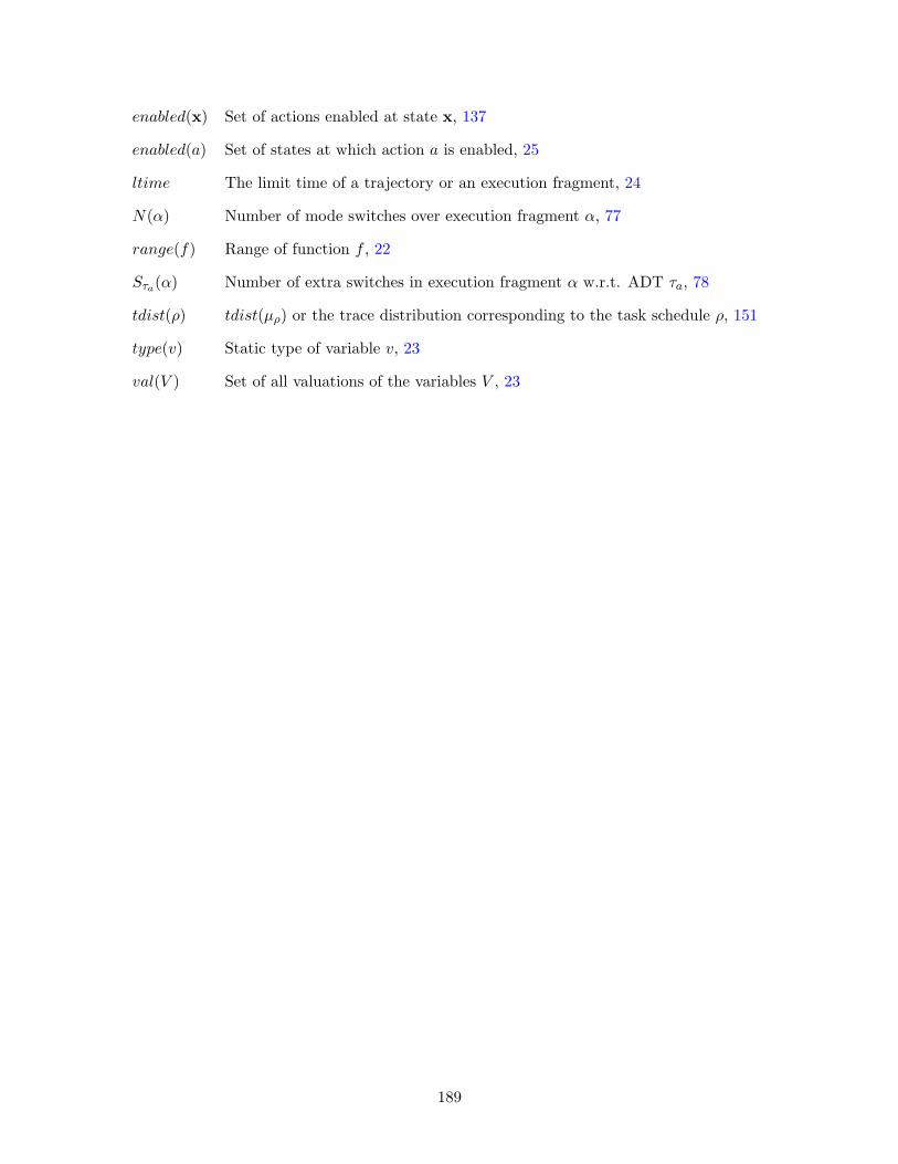
enabled(x) Set of actions enabled at state x, 137
enabled(a) Set of states at which action a is enabled, 25
ltime The limit time of a trajectory or an execution fragment, 24
N(α) Number of mode switches over execution fragment α, 77
range(f) Range of function f , 22
Sτa(α) Number of extra switches in execution fragment α w.r.t. ADT τa, 78
tdist(ρ) tdist(µρ) or the trace distribution corresponding to the task schedule ρ, 151
type(v) Static type of variable v, 23
val(V ) Set of all valuations of the variables V , 23
189

Index
abstraction, see implementationActuator, 62ADT, 77
equivalent, 80automaton
generalized PTIOA, 152PIOA, 160pre-PTIOA, 138Task DPTIOA, 139task-PIOA, 160
Average Dwell Time, see ADT
base, 143basic set, 143Bounce, 38
in PVS , 113Burner, 85
ClockSync, 48compatible, 27composition, 27, 29, 35, 141, 153
in HIOA language, 49of PIOA, 161
compositionality, 12cone, 162
DAI, 30in HIOA language, 47
deadline variable, 40deterministic trajectories, 136Dirac measure, 136dtype, 23
in HIOA language, 41continuous, 30discrete, 30
dynamic type, see dtype
environment, 181environment automaton, 151execution, 26, 140, 161
fragment, 26, 140
probabilistic, 146expansion
of function, 166of relation, 164
external behavior, 151
failure detector, 50, 129flattening, 163formal parameter, see parameterforward simulation relation, 55functions
in HIOA language, 43
Helicopter, 58hierarchical refinement, 12hysteresis
linear, 91scale-independent, 86
HystSwitch, 86
implementation, 27, 29, 35, 151, 153discounted approximate, 178proving inductively, 55uniform approximate, 165
inductive property, 54invariant, 26, 53
in HIOA language, 50in PVS , 117of composed automaton, 55proving inductively, 54
kindsof variables, 40
lifting, 164LinHSwitch, 91Lyapunov stability, see stability
Markov chain, 172metric, 165mode switch, 35, 77
190
NoisySensor, 154
parameter, 39constant, 44type, 40
polymorphism, 40pre-HIOA, 29pre-SHIOA, 34precondition
in HIOA language, 44preconditions
in PVS , 112pseudometric, 165PTIOA, 137PVS strategy, see strategy
reachability, 26reachable state, 26reachable states, 26restriction, 26
safety, 26scheduler, 145semi-ring, 137Sensor, 58SHIOA
initialized, 35, 96linear, 35one-clock initialized, 90rectangular, 35
signature, 43in PVS , 110
simulationdiscounted approximate, 179expanded approximate, 168
simulation relation, 55in HIOA language, 50in PVS , 119
Spec, 50, 130in PVS , 115
stability, 26, 76asymptotic, 76exponential, 77global asymptotic, 76global exponential, 77uniform, 77
stable, 76state models
in HIOA language, 45
in PVS , 110semantics, 30
static type, see typestrategy, 105, 123substitutivity, 152
HA, 28Supervisor, 59switched system, 75switching simulation relation, 80
task correspondence, 164task schedule, 145see Task DPTIOA, 139tasks, 139Two-TaskRace, 130theory instantiation, 120thermostat, 47Thermostat2, 100Thermostat, 47TimedChannel, 47Timeout, 51Timeout
in PVS , 118trace, 26, 161
distribution, 148PTIOA, 140
trace basic set, 145trace distribution, 151trajectories
in HIOA language, 45in PVS , 109, 113
trajectory, 24closed, 24open, 24point, 24
transitionsin HIOA language, 44in PVS , 111, 112
type, 23constructors, 40parameter, 40
typesin HIOA language, 40
valuation, 23variable
continuous, 23discrete, 23
191

variablesin HIOA Language, 39in PVS , 109
vocabulary, 40
where-clause, 38
192
Bibliography
[A+95] R. Alur et al. The algorithmic analysis of hybrid systems. Theoretical Com-puter Science, 138:3–34, 1995.
[ABD+00] Eugene Asarin, Olivier Bournez, Thao Dang, Amir Pnueli, and Oded Maler.Effective synthesis of switching controllers for linear systems. In Proceedingsof IEEE, volume 88, pages 1011–1025, July 2000.
[ACH+95] Rajeev Alur, Costas Courcoubetis, Nicolas Halbwachs, Thomas A. Henzinger,P.-H. Ho, Xavier Nicollin, Alfredo Olivero, Joseph Sifakis, and Sergio Yovine.The algorithmic analysis of hybrid systems. Theoretical Computer Science,138(1):3–34, 1995.
[AD94] Rajeev Alur and David L. Dill. A theory of timed automata. TheoreticalComputer Science, 126:183–235, 1994.
[AHH93] R. Alur, C. Courcoubetis T. A. Henzinger, and P. H. Ho. Hybrid automata: analgorithmic approach to the specification and verification of hybrid systems.In R. L. Grossman, A. Nerode, A. P. Ravn, and H. Rischel, editors, HybridSystems, volume 736 of LNCS, pages 209–229. Springer-Verlag, 1993.
[AHS98] M. Archer, C. Heitmeyer, and S. Sims. TAME: A PVS interface to simplifyproofs for automata models. In Proceedings of UITP ’98, July 1998.
[ALL+06] Myla Archer, HongPing Lim, Nancy Lynch, Sayan Mitra, and Shinya Umeno.Specifying and proving properties of timed I/O automata in the TIOA toolkit.In In Fourth ACM-IEEE International Conference on Formal Methods andModels for Codesign (MEMOCODE’06). IEEE, 2006.
[Alu91] R. Alur. Techniques for automatic verification of real-time systems. PhDthesis, Stanfor University, 1991.
[AP04] Rajeev Alur and George J. Pappas, editors. Hybrid Systems: Computation andControl, 7th International Workshop, HSCC 2004, Philadelphia, PA, USA,March 25-27, 2004, Proceedings, volume 2993 of LNCS. Springer, 2004.
[Arc01] Myla Archer. TAME: PVS Strategies for special purpose theorem proving.Annals of Mathematics and Artificial Intelligence, 29(1/4), February 2001.
[ASL93] P. J. Antsakis, J. A. Stiver, and M. D. Lemmon. Hybrid system modelingand autonomous control systems. In R. L. Grossman et al., editors, HybridSystems, volume 736 of LNCS, New York, 1993.
193

[AVM03] Myla Archer, Ben Di Vito, and Cesar Munoz. Developing user strategies inpvs: A tutorial. In STRATA 2003, Rome, Italy, 2003.
[BBM98] M. Branicky, V. Borkar, and S. Mitter. A unified framework for hybrid control:model and optimal control theory. IEEE Transactions on Automatic Control,43(1):31–45, 1998.
[BCG06] C. Baier, F. Ciesinski, and M. Grer. ProbMela and model checking markovdecision processes. In ACM Performance Evaluation Review on Performanceand Verification, 2006. to appear.
[BCT02] Alexandre M. Bayen, Eva Cruck, and Claire Tomlin. Guaranteed overap-proximations of unsafe sets for continuous and hybrid systems: solving thehamilton-jacobi equation using viability techniques. In Tomlin and Green-street [TG02], pages 90–104.
[BGL02] A. Bogdanov, S. Garland, and N. Lynch. Mechanical translation of I/O au-tomaton specifications into first-order logic. In Formal Techniques for Net-worked and Distributed Sytems - FORTE 2002 : 22nd IFIP WG 6.1 Interna-tional Conference, pages 364–368, Texas, Houston, USA, November 2002.
[BGM93] A. Back, J. Guckenheimer, and M. Myers. A dynamical simulation facility forhybrid systems. In R. L. Grossman et al., editors, Hybrid Systems, volume736 of LNCS, New York, 1993.
[BLB05] Manuela L. Bujorianu, John Lygeros, and Marius C. Bujorianu. Bisimulationfor general stochastic hybrid systems. In Morari and Thiele [MT05], pages198–214.
[BO83] M. Ben-Or. Another advantage of free choice: Completely asynchronous agree-ment protocols. In PODC, pages 27–30, Montreal, Canada, August 1983.
[Bra95] M. Branicky. Studies in hybrid systems: modeling, analysis, and control. PhDthesis, MIT, Cambridge, MA, June 1995.
[Bro94] R. W. Brockett. Hybrid models for motion control systems. In H. L. Trentel-man and J. C. Willems, editors, Essays in Control: Perspectives in the Theoryand its Applications, pages 20–53, Boston, 1994. Birkhauser.
[BS67] N. P. Bhatia and G. P. Szego. Dynamical Systems: Stability Theory andApplications, volume 35 of Lecture notes in mathematics. Springer-Verlag,Berlin; New York, 1967.
[C. 96] C. Baier. Polynomial-time algorithms for testing probabilistic bisimulationand simulation. In Rajeev Alur and Thomas A. Henzinger, editors, Proceed-ings of the Eighth International Conference on Computer Aided VerificationCAV, volume 1102, pages 50–61, New Brunswick, NJ, USA, / 1996. SpringerVerlag.
[CCK+05] Ran Canetti, Ling Cheung, Dilsun Kirli, Moses Liskov, Olivier PereiraNancy Lynch, and Roberto Segala. Using probabilistic I/O automata to an-alyze an oblivious transfer protocol. Technical report, MIT LCS Technical
194
Reports - MIT-LCS-TR-1001, August 2005. Also in MIT CSAIL TechnicalReports - MIT-CSAIL-TR-2005-055.
[CCK+06a] Ran Canetti, Ling Cheung, Dilsun Kaynar, Moses Liskov, Nancy Lynch,Olivier Pereira, and Roberto Segala. Task-structured Probabilistic I/O Au-tomata. In Proceedings of the 8th International Workshop on Discrete EventSystems – WODES’2006, 2006. IEEE catalog number 06EX1259.
[CCK+06b] Ran Canetti, Ling Cheung, Dilsun Kaynar, Moses Liskov, Nancy Lynch,Olivier Pereira, and Roberto Segala. Task-structured probabilistic I/O au-tomata. Technical Report MIT-CSAIL-TR-2006-060, Massachusetts Instituteof Technology, Cambridge, MA, September 2006.
[CCK+06c] Ran Canetti, Ling Cheung, Dilsun Kaynar, Moses Liskov, Nancy Lynch,Olivier Pereira, and Roberto Segala. Time-bounded task-PIOAs: a frame-work for analyzing security protocols. In 20th International Symposium onDistributed Computing, (DISC 2006), volume 4167 of LNCS, pages 238–253.Springer, 2006.
[CCK+06d] Ran Canetti, Ling Cheung, Dilsun Kaynar, Moses Liskov, Nancy Lynch,Olivier Pereira, and Roberto Segala. Using task-structured probabilistic I/Oautomata to analyze an oblivious transfer protocol. Technical Report MIT-CSAIL-TR-2006-019, Massachusetts Institute of Technology, Cambridge, MA,March 2006. Available from http://theory.csail.mit.edu/tds/papers/Kirli/TR-2006-019.pdf.
[CES86] E. Clarke, E. A. Emerson, and A. P. Sistla. Automatic verification of finite-state concurrent systems using temporal logic specifications. ACM Transac-tions on Programming Languages and Systems, 8(2):244–263, 1986.
[Che06] L. Cheung. Reconciling nondeterministic and probabilistic choices. PhD thesis,ICIS, Radboud University Nijmegen, The Netherlands, 2006.
[CL04] D. Chatterjee and D. Liberzon. On stability of stochastic switched systems. InProceedings of the 43rd Conference on Decision and Control, pages 4125–4127,Paradise Island, Bahamas, December 2004.
[CL06] Debasish Chatterjee and Daniel Liberzon. Stability analysis of deterministicand stochastic switched systems via a comparison principle and multiple lya-punov functions. SIAM Journal on Control and Optimization, 45(1):174–206,March 2006.
[CLMT05] Gregory Chockler, Nancy Lynch, Sayan Mitra, and Joshua Tauber. Provingatomicity: an assertional approach. In Pierre Fraigniaud, editor, Proceedingsof Nineteenth International Symposium on Distributed Computing (DISC’05),volume 3724 of LNCS, pages 152 – 168, Cracow, Poland, September 2005.Springer.
[CLR90] Thomas H. Cormen, Charles E. Leiserson, and Ronald L. Rivest. Introductionto Algorithms. MIT Press/McGraw-Hill, 1990.
195

[CLSV04] L. Cheung, N. A. Lynch, R. Segala, and F. Vaandrager. Switched probabilisticI/O automata. In First International Colloquium on Theoretical Aspects ofComputing, July 2004.
[COR+95] Judy Crow, Sam Owre, John Rushby, Natarajan Shankar, and MandayamSrivas. A tutorial introduction to PVS. Presented at WIFT ’95: Workshopon Industrial-Strength Formal Specification Techniques, Boca Raton, Florida,April 1995. Available, with specification files, at http://www.csl.sri.com/wift-tutorial.html.
[Cru91] Rene L. Cruz. A calculus for network delay, part i: Network elements inisolation. IEEE Transactions on Information Theory, 37(1):114–131, 1991.
[CSKN05] Stefano Cattani, Roberto Segala, Marta Z. Kwiatkowska, and Gethin Nor-man. Stochastic transition systems for continuous state spaces and non-determinism. In FoSSaCS’05, volume 3441 of LNCS, pages 125–139. Springer,2005.
[dA97] Luca de Alfaro. Formal Verification of Probabilistic Systems. PhD thesis,Stanford University, CA, 1997. Technical Report STAN-CS-TR-98-1601.
[Dav83] Martin Davis. The prehistory and early history of automated deduction.Automated Reasoning, 1:1–28, 1983.
[Dav93] M. H. A. Davis. Markov Models and Optimization. Chapman & Hall, 1993.
[DDLP05] Vincent Danos, Jose Desharnais, Francois Laviolette, and Prakash Panan-gaden. Bisimulation and cocongruence for probabilistic systems. Informationand Computation, Special issue for selected papers from CMCS04, 2005.
[Dev99] Marco Devillers. Translating IOA automata to PVS. Technical ReportCSI-R9903, Computing Science Institute, University of Nijmegen, Febru-ary 1999. Available at http://www.cs.ru.nl/research/reports/info/CSI-R9903.html.
[DGJP03] Josee Desharnais, Vineet Gupta, Radha Jagadeesan, and Prakash Panan-gaden. Approximating labelled markov processes. Inf. Comput., 184(1):160–200, 2003.
[DGJP04] Jose Desharnais, Vineet Gupta, Radha Jagadeesan, and Prakash Panangaden.Metrics for labelled markov processes. Theor. Comput. Sci., 318(3):323–354,2004.
[DGRV00] M. Devillers, D. Griffioen, J. Romijn, and F. Vaandrager. Verification ofa leader election protocol—formal methods applied to IEEE 1394. FormalMethods in System Design, 16(3):307–320, June 2000.
[DJGP02] J. Desharnais, R. Jagadeesan, V. Gupta, and P. Panangaden. The metric ana-logue of weak bisimulation for probabilistic processes. In Proceedings of the17th Annual IEEE Symposium on Logic in Computer Science (LICS), Copen-hagen, Denmark, 22-25 July 2002, pages 413–422. IEEE Computer Society,2002.
196

[DL97] Ekaterina Dolginova and Nancy Lynch. Safety verification for automatedplatoon maneuvers: A case study. In HART’97 (International Workshopon Hybrid and Real-Time Systems), volume 1201 of LNCS. Springer Verlag,March 1997.
[DLL97] R. DePrisco, Butler Lampson, and Nancy Lynch. Revisitng the paxos algo-rithm. In Distributed Algorithms 11th Workshop WDAG’97, pages 111–125,Berlin-Heidelberg, 1997.
[Dol00] Shlomi Dolev. Self-stabilization. MIT Press, Cambridge, MA, USA, 2000.
[Doo53] J. L. Doob. Stochastic Processes. John Wiley & Sons, Inc., New York, 1953.
[DOT06] A. Dhama, J. Oehlerking, and O. Theel. Verification of orbitally self-stabilizing distributed algorithms using lyapunov functions and poincaremaps. In 12th Intl. Conf. on Parallel and Distributed Systems (ICPADS’06),pages 23–30, 2006.
[Dud76] R. M. Dudley. Probabilities and Metrics:Convergence of laws on metric spaces,with a view to statistical testing. Number 45 in Lecture Notes Series. AarhusUniversitet, June 1976.
[Dud89] R. M. Dudley. Real Analysis and Probability. Wadsworth, Belmont, Calif,1989.
[ES03] S. Smolka E. Stark, R. Cleaveland. A process-algebraic language for proba-bilistic I/O automata. In Proc. CONCUR 03, volume 2761 of LNCS 2761,pages 189–203, Marseille, France, September 2003. Springer.
[FDGL07] Rui Fan, Ralph E. Droms, Nancy D. Griffeth, and Nancy A. Lynch. The dhcpfailover protocol: A formal perspective. In Formal Techniques for Networkedand Distributed Systems - FORTE 2007, pages 211–226, 2007.
[FK98] Enrique D. Ferreira and Bruce H. Krogh. Switching controllers based onneural network: Estimates of stability regions and controller performance. InHybrid Systems: Computation and Control 1998, pages 126–142, 1998.
[Flo67] Robert Floyd. Assigning meanings to programs. In Sympyposium on Ap-plied Mathematics. Mathematical Aspects of Computer Science, pages 19–32.American Mathematical Society, 1967.
[Fre05] Goran Frehse. Phaver: Algorithmic verification of hybrid systems past hytech.In Morari and Thiele [MT05], pages 258–273.
[GCMF93] Gordon, M. J. C., Melham, and Thomas F. Introduction to HOL: A theoremproving environment for higher order logic. Cambridge University Press, 1993.
[GG91] Stephen J. Garland and John V. Guttag. A guide to LP, the Larch prover.Technical report, DEC Systems Research Center, 1991. Available at http://nms.lcs.mit.edu/Larch/LP.
[GGC81] Keith O. Geddes, Gaston H. Gonnet, and Bruce W. Char. Maple user’s man-ual. Technical Report CS-81-25, Computer Science Department, Universityof Waterloo, Waterloo, Ontario, Canada, 1981.
197

[Gir81] M. Giry. A categorical approach to probability theory. In B. Banaschewski,editor, Categorical Aspects ofTopology and Analysis, number 915 in LectureNotes in Mathematics, pages 68–85. Springer-Verlag, 1981.
[GJP04] Vineet Gupta, Radha Jagadeesan, and Prakash Panangaden. Approximatereasoning for real-time probabilistic processes. The Quantitative Evaluationof Systems, First International Conference on (QEST’04), 00:304–313, 2004.
[GJP06] Antoine Girard, A. Agung Julius, and George J. Pappas. Approximate sim-ulation relations for hybrid systems. In IFAC Analysis and Design of HybridSystems, Alghero, Italy, June 2006.
[GLTV03] S. Garland, N. Lynch, J. Tauber, and M. Vaziri. IOA User Guide and Refer-ence Manual. MIT Computer Science and Artificial Intelligence Laboratory,Cambridge, MA, 2003. Available at http://theory.lcs.mit.edu/tds/ioa.html.
[GMY+07] Radu Grosu, Sayan Mitra, Pei Ye, Emilia Entcheva, I. V. Ramakrishnan, andScott A. Smolka. Learning cycle-linear hybrid automata for excitable cells. InHSCC, pages 245–258, 2007.
[GNU] GNU. GLPK - GNU linear programming kit. Available from http://www.gnu.org/directory/libs/glpk.html.
[GP05] Antoine Girard and George J. Pappas. Approximation metrics for discreteand continuous systems. In IEEE Transactions on Automatic Control, 2005.
[GPS06] Marc Girault, Guillaume Poupard, and Jacques Stern. On the fly authenti-cation and signature schemes based on groups of unknown order. Journal ofCryptology, 19(4):463—487, 2006.
[Hen96] Thomas Henzinger. The theory of hybrid automata. In Proceedings of the 11thAnnual IEEE Symposium on Logic in Computer Science (LICS ’96), pages278–292, New Brunswick, New Jersey, 1996.
[Her02] Holger Hermanns. Interactive Markov Chains : The Quest for QuantifiedQuality. Springer Berlin / Heidelberg, 2002.
[Hes04] Joao P. Hespanha. Stochastic hybrid systems: Application to communicationnetworks. In Alur and Pappas [AP04], pages 387 – 401.
[HHWT97] Thomas A. Henzinger, Pei-Hsin Ho, and Howard Wong-Toi. Hytech: A modelchecker for hybrid systems. In Computer Aided Verification (CAV ’97), vol-ume 1254 of LNCS, pages 460–483, 1997.
[HK96] Thomas A. Henzinger and Peter W. Kopke. State equivalences for rectan-gular hybrid automata. In International Conference on Concurrency Theory(CONCUR‘96), pages 530–545, 1996.
[HKNP06] A. Hinton, M. Kwiatkowska, G. Norman, and D. Parker. PRISM: A tool forautomatic verification of probabilistic systems. In H. Hermanns and J. Pals-berg, editors, Proc. 12th International Conference on Tools and Algorithms
198

for the Construction and Analysis of Systems (TACAS’06), volume 3920 ofLNCS, pages 441–444. Springer, 2006.
[HKPV95] Thomas A. Henzinger, Peter W. Kopke, Anuj Puri, and Pravin Varaiya.What’s decidable about hybrid automata? In ACM Symposium on Theory ofComputing, pages 373–382, 1995.
[HKPV98] Thomas A. Henzinger, Peter W. Kopke, Anuj Puri, and Pravin Varaiya.What’s decidable about hybrid automata? Journal of Computer and Sys-tem Sciences, 57:94–124, 1998.
[HL94] Connie Heitmeyer and Nancy Lynch. The generalized railroad crossing: Acase study in formal verification of real-time system. In Proceedings of the15th IEEE Real-Time Systems Symposium, San Juan, Puerto Rico, December1994. IEEE Computer Society Press.
[HLM03] J.P. Hespanha, D. Liberzon, and A.S. Morse. Hysteresis-based switching algo-rithms for supervisory control of uncertain systems. Automatica, 39:263–272,2003.
[HLS00] J. Hu, J. Lygeros, and S. Sastry. Towards a theory of stochastic hybridsystems. In N. Lynch and B. H. Krogh, editors, Hybrid Systems: Computationand Control, 3rd Int. Workshop (HSCC 2000), volume 1790 of LNCS, pages160–173, 2000, 2000.
[HM99] J.P. Hespanha and A. Morse. Stability of switched systems with average dwell-time. In Proceedings of 38th IEEE Conference on Decision and Control, pages2655–2660, 1999.
[HNSY94] T. A. Henzinger, X. Nicollin, J. Sifakis, and S. Yovine. Symbolic model check-ing for real-time systems. Information and Computation, 111(2):193–244,1994.
[HR95] M. Hennessy and T. Regan. A process algebra for timed systems. Informationand Computation, 117:221–239, 1995.
[HT06] Joao P. Hespanha and Ashish Tiwari, editors. Hybrid Systems: Computationand Control, 9th International Workshop, HSCC 2006, Santa Barbara, CA,USA, March 29-31, 2006, Proceedings, volume 3927 of LNCS. Springer, 2006.
[Int06] SRI International. The PVS bibliography, 2006. http://pvs.csl.sri.com/papers/pvs-bib/pvs-bib.html.
[JS90] C.-C. Jou and S. A. Smolka. Equivalences, congruences and complete approx-imations for probabilistic processes. In CONCUR 90, number 458 in LNCS.Springer-Verlag, 1990.
[Kan] L. Kantorovich. On the transfer of masses. Doklady Akademii Nauk,37(i2):227–229.
[Kha02] H. K. Khalil. Nonlinear Systems. Prentice Hall, New Jersey, 3rd edition, 2002.
199

[KLMG05] D. Kaynar, N. Lynch, S. Mitra, and S. Garland. TIOA Language. MITComputer Science and Artificial Intelligence Laboratory, Cambridge, MA,2005.
[KLSV03] Dilsun K. Kaynar, Nancy Lynch, Roberto Segala, and Frits Vaandrager.Timed I/O automata: A mathematical framework for modeling and analyz-ing real-time system. In RTSS 2003: The 24th IEEE International Real-TimeSystems Symposium, Cancun,Mexico, December 2003.
[KLSV04] D. Kaynar, N. Lynch, R. Segala, and F. Vaandrager. The theory of timedI/O automata. Technical Report MIT/LCS/TR-917a, MIT Laboratory forComputer Science, 2004. Available at http://theory.lcs.mit.edu/tds/reflist.html.
[KLSV05] Dilsun K. Kaynar, Nancy Lynch, Roberto Segala, and Frits Vaandrager. TheTheory of Timed I/O Automata. Synthesis Lectures on Computer Science.Morgan Claypool, November 2005. URL:http://www.morganclaypool.com/doi/abs/10.2200/S00006ED1V01Y200508CSL001. Also available as TechnicalReport MIT-LCS-TR-917.
[KN96] Marta Z. Kwiatkowska and Gethin Norman. Probabilistic metric semanticsfor a simple language with recursion. In MFCS ’96: Proceedings of the 21stInternational Symposium on Mathematical Foundations of Computer Science,pages 419–430, London, UK, 1996. Springer-Verlag.
[KNSW04] M. Kwiatkowska, G. Norman, J. Sproston, and F. Wang. Symbolicmodel checking for probabilistic timed automata. In In Proc. FORMAT-S/FTRTFT’04, volume 3253 of LNCS, pages 293–308. Springer-Verlag,September 2004.
[Lib03] Daniel Liberzon. Switching in Systems and Control. Systems and Control:Foundations and Applications. Birkhauser, Boston, June 2003.
[Lim01] Hongping Lim. Translating timed I/O automata specifications for theoremproving in PVS. Master’s thesis, Massachusetts Institute of Technology,February 2001.
[LKLM05] Hongping Lim, Dilsun Kaynar, Nancy Lynch, and Sayan Mitra. Translatingtimed I/O automata specifications for theorem proving in pvs. In Proceedingsof Formal Modelling and Analysis of Timed Systems (FORMATS’05), number3829 in LNCS, Uppsala, Sweden, September 2005. Springer.
[LL96] Gunter Leeb and Nancy Lynch. Proving safety properties of the steam boilercontroller. In Egon Boerger Jean Raymond Abrial and Hans Langmaack,editors, Formal Methods for Industrial Applications: Specifying and Program-ming the Steam Boiler Control, volume 11654 of LNCS, 1996.
[LLL99] Carolos Livadas, John Lygeros, and Nancy A. Lynch. High-level modelingand analysis of TCAS. In Proceedings of the 20th IEEE Real-Time SystemsSymposium (RTSS’99),Phoenix, Arizona, pages 115–125, December 1999.
200

[LMMS98] P. Lincoln, J. Mitchell, M. Mitchell, and A. Scedrov. A probabilistic poly-time framework for protocol analysis. In CCS ’98: Proceedings of the 5thACM conference on Computer and communications security, pages 112–121,New York, NY, USA, 1998. ACM Press.
[LMN] Nancy Lynch, Sayan Mitra, and Tina Nolte. Motion coordination using virtualnodes. In Proceedings of 44th IEEE Conference on Decision and Control(CDC05), Seville, Spain, December.
[LPY99] Gerardo Lafferriere, George J. Pappas, and Sergio Yovine. A new class ofdecidable hybrid systems. In HSCC ’99: Proceedings of the Second Inter-national Workshop on Hybrid Systems, pages 137–151, London, UK, 1999.Springer-Verlag.
[LS91] Kim Guldstrand Larsen and Arne Skou. Bisimulation through probabilistictesting. Inf. Comput., 94(1):1–28, 1991.
[LSV03] Nancy Lynch, Roberto Segala, and Frits Vaandrager. Hybrid I/O automata.Information and Computation, 185(1):105–157, August 2003.
[LTS99] John Lygeros, Claire Tomlin, and Shankar Sastry. Controllers for reachabilityspecifications for hybrid systems. In Automatica, volume 35, March 1999.
[Lue79] David G. Luenberger. Introduction to Dynamic Systems: Theory, Models,and Applications. John Wiley and Sons, Inc., New York, 1979.
[LV96] Nancy Lynch and Frits Vaandrager. Forward and backward simulations - partII: Timing-based systems. Information and Computation, 128(1):1–25, July1996.
[Lyn96a] Nancy Lynch. A three-level analysis of a simple acceleration maneuver, withuncertainties. In Proceedings of the Third AMAST Workshop on Real-TimeSystems, pages 1–22, Salt Lake City, Utah, March 1996. World Scientific Pub-lishing Company.
[Lyn96b] Nancy A. Lynch. Distributed Algorithms. Morgan Kaufmann Publishers Inc.,1996.
[MA03] Sayan Mitra and Myla Archer. Developing strategies for specialized theoremproving about untimes, timed, and hybrid I/O automata. In STRATA 2003,Rome, Italy, 2003.
[MA04] Sayan Mitra and Myla Archer. Reusable pvs proof strategies for proving ab-straction properties of I/O automata. In STRATEGIES 2004, IJCAR Work-shop on strategies in automated deduction, Cork, Ireland, July 2004.
[MA05] Sayan Mitra and Myla Archer. PVS strategies for proving abstractionproperties of automata. Electronic Notes in Theoretical Computer Science,125(2):45–65, 2005.
[Mat74] Mathlab Group. MACSYMA primer: introductory section. Cambridge, MA,USA, 1974.
201

[Meg01] Alexandre Megretski. On automatic search for invariants of hybrid systems.In American Control Conference, pages 217–223, Arlington, VA, 2001.
[Mit01] Sayan Mitra. HIOA - a specification language for hybrid Input/Output au-tomata. Master’s thesis, Department of Computer Science and Automation,IISc, Indian Institute of Science, Bangalore, 2001.
[ML06] Sayan Mitra and Nancy Lynch. Approximate simulations for task-structuredprobabilistic I/O automata. In LICS workshop on Probabilistic Automata andLogics (PAul06), Seattle, WA, August 2006.
[ML07] Sayan Mitra and Nancy Lynch. Proving approximate implementation relationsfor probabilistic I/O automata. Electronic Notes in Theoretical ComputerScience, 174(8):71–93, 2007.
[MLL06] Sayan Mitra, Daniel Liberzon, and Nancy Lynch. Verifying average dwell timeby solving optimization problems. In Hespanha and Tiwari [HT06], pages476–490. Full version: http://theory.lcs.mit.edu/~mitras/research/hscc06_full.pdf.
[MM01] C. Munoz and M. Mayero. Real automation in the field. Technical ReportNASA/CR-2001-211271 Interim ICASE Report No. 39, ICASE-NASA Lang-ley, ICASE Mail Stop 132C, NASA Langley Research Center, Hampton VA23681-2199, USA, December 2001.
[MMS05] J. Misra, G. Morrisett, and N. Shankar, editors. Workshop on The VerificationGrand Challenge, SRI International, Menlo Park, CA, 2005.
[MMT91] Michael Merritt, Francesmary Modugno, and Mark Tuttle. Time constrainedautomata. In J. C. M. Baeten andJ. F. Goote, editor, CONCUR ’91: 2ndInternational Conference of Concurrency Theory, volume 527, pages 408–423,1991.
[Mor96] A. S. Morse. Supervisory control of families of linear set-point controllers, part1: exact matching. IEEE Transactions on Automatic Control, 41:1413–1431,1996.
[MOW04] M. W. Mislove, J. Ouaknine, and J. Worrell. Axioms for probability andnondeterminism. ENTCS, 2004.
[MP81] Z. Manna and A. Pnueli. The Correctness problem in Computer Science,chapter The temporal framework for concurrent programs. Academic Press,1981.
[MP03] Oded Maler and Amir Pnueli, editors. Hybrid Systems: Computation andControl, 6th International Workshop, HSCC 2003 Prague, Czech Republic,April 3-5, 2003, Proceedings, volume 2623 of LNCS. Springer, 2003.
[MT05] Manfred Morari and Lothar Thiele, editors. Hybrid Systems: Computationand Control, 8th International Workshop, HSCC 2005, Zurich, Switzerland,March 9-11, 2005, Proceedings, volume 3414 of LNCS. Springer, 2005.
202

[MWLF03] Sayan Mitra, Yong Wang, Nancy Lynch, and Eric Feron. Safety verificationof model helicopter controller using hybrid Input/Output automata. In Malerand Pnueli [MP03], pages 343–358.
[MWMW04] D. Pavlovic M. W. Mislove, J. Ouaknine and J. Worrell. Duality for labelledmarkov processes. In Proceedings of FOSSACS 04, volume 2987 of LNCS.Springer, 2004.
[NA02] Mikhail Nesterenko and Anish Arora. Stabilization-preserving atomicity re-finement. J. Parallel Distrib. Comput., 62(5):766–791, 2002.
[NK93] A. Nerode and W. Kohn. Models for hybrid systems: Automata, topologies,stability. In R. L. Grossman et al., editors, Hybrid Systems, volume 736 ofLNCS, New York, 1993.
[NW03] Toh Ne Win. Theorem-proving distributed algorithms with dynamic analysis.Master’s thesis, Massachusetts Institute of Technology, Cambridge, MA, May2003.
[Oga97] Katsuhiko Ogata. Modern control engineering (3rd ed.). Prentice-Hall, Inc.,Upper Saddle River, NJ, USA, 1997.
[ORR+96] S. Owre, S. Rajan, J.M. Rushby, N. Shankar, and M.K. Srivas. PVS: Com-bining specification, proof checking, and model checking. In Rajeev Alur andThomas A. Henzinger, editors, Computer-Aided Verification, CAV ’96, num-ber 1102 in LNCS, pages 411–414, New Brunswick, NJ, July/August 1996.Springer-Verlag.
[ORSSC98] Sam Owre, John Rushby, N. Shankar, and David Stringer-Calvert. PVS: anexperience report. In Dieter Hutter, Werner Stephan, Paolo Traverso, andMarkus Ullman, editors, Applied Formal Methods—FM-Trends 98, volume1641 of LNCS, pages 338–345, Boppard, Germany, oct 1998. Springer-Verlag.
[OS01] S. Owre and N. Shankar. Theory interpretations in PVS. Technical report,Computer Science Lab., SRI Intl., Menlo Park, CA, 2001.
[OSRSC99] S. Owre, N. Shankar, J. M. Rushby, and D. W. J. Stringer-Calvert. PVSLanguage Reference. Computer Science Laboratory, SRI International, MenloPark, CA, September 1999.
[Pau93] Lawrence C. Paulson. The Isabelle reference manual. Technical Report 283,University of Cambridge, 1993.
[Pnu77] A. Pnueli. The temporal logic of programs. In IEEE Symposium on Founda-tions of Computer Science, pages 46–77, 1977.
[Qua] Quanser. Control challenges: 3 DOF helicopter http://www.quanser.com/english/html/products/fs_product_challenge.asp?lang_code=english&pcat_code=exp-spe&prod_code=S1-3dofheli&tmpl=1.
[Rac91] Svetlozar T. Rachev. Probability metrics and the stability of stochastic models.John Wiley & Sons, 1991.
203

[Seg95a] R. Segala. A compositional trace-based semantics for probabilistic automata.In Proceedings of the 6th International Conference on Concurrency Theory(CONCUR ’ 95), volume 962 of LNCS, pages 234–248, Philadelphia, PA,USA, August 1995.
[Seg95b] Roberto Segala. Modeling and Verification of Randomized Distributed Real-Time Systems. PhD thesis, Laboratory for Computer Science, MassachusettsInstitute of Technology, June 1995.
[Seg96] R. Segala. Testing probabilistic automata. In Proceedings of the 7th Interna-tional Conference on Concurrency Theory (CONCUR ’ 96), volume 1119 ofLNCS, pages 299–314, Pisa, Italy, August 1996.
[SORSC99] N. Shankar, S. Owre, J. M. Rushby, and D. W. J. Stringer-Calvert. PVSProver Guide. Computer Science Laboratory, SRI International, Menlo Park,CA, September 1999.
[SSM04] Sriram Sankaranarayanan, Henny Sipma, and Zohar Manna. Constructinginvariants for hybrid systems. In Alur and Pappas [AP04], pages 539–554.
[Sta03] E. Stark. On behavior equivalence for probabilistic I/O automata and itsrelationship to probabilistic bisimulation. Journal of Automata, Languages,and Combinatorics, 8(2):361–395, 2003.
[SvdS05] Stefan Strubbe and A. J. van der Schaft. Bisimulation for communicat-ing piecewise deterministic markov processes (cpdps). In Morari and Thiele[MT05], pages 623–639.
[TEM07] Tempo toolset, version 0.1.9 beta, August 2007. http://www.veromodo.com/tempo/.
[TG02] Claire Tomlin and Mark R. Greenstreet, editors. Hybrid Systems: Compu-tation and Control, 5th International Workshop, HSCC 2002, Stanford, CA,USA, March 25-27, 2002, Proceedings, volume 2289 of LNCS. Springer, 2002.
[The04] The Coq Development Team. The Coq Proof Assistant Reference Manual –Version V8.0, April 2004. http://coq.inria.fr.
[TK02] Ashish Tiwari and Gaurav Khanna. Series of abstractions for hybrid au-tomata. In Tomlin and Greenstreet [TG02], pages 465–478.
[TPL02] Paulo Tabuada, George J. Pappas, and Pedro U. Lima. Composing abstrac-tions of hybrid systems. In Tomlin and Greenstreet [TG02], pages 436–450.
[UL07] Shinya Umeno and Nancy A. Lynch. Safety verification of an aircraft landingprotocol: A refinement approach. In HSCC, pages 557–572, 2007.
[vBMOW03] F. van Breugel, M. Mislove, J. Ouaknine, and J. B. Worrell. An intrinsiccharacterization of approximate probabilistic bisimilarity. In Proceedings ofFOSSACS 03, LNCS. Springer, 2003.
[vBMOW05] F. van Breugel, M. W. Mislove, J. Ouaknine, and J. Worrell. Domain theory,testing and simulation for labelled markov processes. Theoretical ComputerScience, 2005.
204

[vBW01a] Franck van Breugel and James Worrell. An algorithm for quantitative ver-ification of probabilistic transition systems. In CONCUR ’01: Proceedingsof the 12th International Conference on Concurrency Theory, pages 336–350,London, UK, 2001. Springer-Verlag.
[vBW01b] Franck van Breugel and James Worrell. Towards quantitative verificationof probabilistic transition systems. In ICALP ’01: Proceedings of the 28thInternational Colloquium on Automata, Languages and Programming,, pages421–432, London, UK, 2001. Springer-Verlag.
[VCL06] L. Vu, D. Chatterjee, and D. Liberzon. Input-to-state stability of switchedsystems and switching adaptive control. Automatica, 2006.
[vdSS00] A. van der Schaft and H. Schumacher. An Introduction to Hybrid DynamicalSystems. Springer, London, 2000.
[Vit02] Ben Di Vito. A PVS prover strategy package for common manipulations.Technical report, NASA Langley Research Center, 2002.
[Wil90] H.P. Williams. Model building in mathematical programming. J. Wiley, NewYork, 1990. third edition.
[WIM+02] Yong Wang, Masha Ishutkina, Sayan Mitra, Nancy A. Lynch, and EricFeron. Design of Supervisory Safety Control for 3DOF Helicopter usingHybrid I/O Automata, 2002. http://gewurtz.mit.edu/ishut/darpa_sec_mit/papers/quanser.ps.
[WL96] H. B. Weinberg and Nancy Lynch. Correctness of vehicle control systems– a case study. In 17th IEEE Real-Time Systems Symposium, pages 62–72,Washington, D. C., December 1996.
[WLD95] H. B. Weinberg, Nancy Lynch, and Norman Delisle. Verification of automatedvehicle protection systems. In T. Henzinger R. Alur and E. Sontag, editors,Hybrid Systems III: Verification and Control Workshop on Verification andControl of Hybrid Systems), volume 1066 of LNCS, pages 101–113. Springer-Verlag, October 1995.
[ZHYM00] G. Zhai, B. Hu, K. Yasuda, and A. Michel. Stability analysis of switched sys-tems with stable and unstable subsystems: An average dwell time approach. InProceedings of the 2000 American Control Conference (2000), chicago,illinois,2000.
205